Fault-Type Identification in New-Type Power Systems Using Online Dictionary Learning and an STP–Attention Spiking Neural Network

Abstract

With the large-scale integration of renewable energy resources into power grids, fault behaviors in new power systems have become more frequent and more complex. To address the difficulty of fault feature extraction under limited measurement configurations, this paper proposes a fault type identification method that combines online dictionary learning (ODL), compressed sensing, and an improved spiking neural network (SNN). First, the mechanisms of typical short-circuit and branch open-circuit faults are analyzed to provide a physical basis for feature construction. Then, an adaptive overcomplete dictionary is built through ODL to obtain sparse representations of fault signals. Finally, short-term plasticity (STP) and an attention mechanism are introduced into the SNN to enhance temporal adaptation and feature selectivity. Simulations on the IEEE 33-bus system evaluate bus- and line-fault classification under different fault locations and simulated noise levels. In the baseline simulations, the overall accuracies were 88.93% for bus faults and 82.48% for line faults, with corresponding macro-F1 scores of 88.83% and 82.38%.

1. Introduction

The large-scale integration of renewable energy resources is accelerating the development of new-type power systems and increasing the importance of advanced sensing, situational awareness, and resilient operation [1,2]. In active distribution networks, distributed generation and power-electronic interfaces introduce stronger variability and more complex transient behavior. Accurate fault-type classification is therefore an important requirement for secure and reliable system operation [2,3].

Fault identification approaches reported in previous studies can generally be divided into mechanism-oriented methods and data-driven approaches. Mechanism-oriented methods rely on the inherent electrical characteristics of power systems, where fault information is extracted through the analysis of network topology, sequence components, impedance/admittance characteristics, and conventional protection principles. Machine-learning and deep-learning approaches have been applied to distribution-system and transmission-line fault detection and classification [3,4]. phasor measurement unit (PMU)-based convolutional and deep neural-network methods have also been developed for wide-area faulted-line localization and power-system event recognition [5,6,7]. In addition, event-driven neuromorphic computing and spiking-neural-network approaches have shown potential for sparse, time-dependent power-system disturbance classification [8,9].

Despite these advances, purely data-driven methods may have limited physical interpretability and may be sensitive to operating conditions, measurement configurations, and noise. Combining mechanism analysis with adaptive feature learning is therefore attractive. Online dictionary learning (ODL) and compressed sensing provide a basis for adaptive sparse representation [10,11], while unsupervised spike-timing-dependent plasticity, short-term synaptic plasticity, and attention mechanisms provide complementary temporal and feature-selective modeling capabilities [12,13,14].

Conventional signal-processing methods generally rely on predefined basis functions, which may not adapt sufficiently to fault signals with nonstationary and multi-timescale characteristics. An online learned dictionary can update its atoms according to incoming samples and obtain sparse representations that preserve discriminative fault information [10]. The resulting sparse features are also compatible with event-driven spiking computation, which can exploit temporal sparsity and local synaptic adaptation [12,13].

Recent studies have investigated sensing and perception technologies for new-type power systems [1], explored artificial intelligence-based approaches for resilient operation [2], and applied machine learning techniques to fault diagnosis in converter-dominated distribution systems [3]. PMU-based CNN models have demonstrated the capability of extracting fault patterns directly from synchronized measurements [5]. Meanwhile, physics-based PMU diagnosis methods maintain stronger connections with network characteristics and fault mechanisms [15]. A recent real-time digital simulator (RTDS)-based study employed distribution-level PMU current data containing pre-fault and fault cycles with deep CNNs, achieving promising performance in fault classification and localization [16]. However, these end-to-end learning methods usually require sufficient labeled samples and provide limited insight into the physical meaning of extracted features.

Therefore, improving the interpretability and adaptability of fault diagnosis methods remains an important issue. Neural additive models have been applied to enhance the interpretability of PMU placement and faulted-line localization [17]; however, their application mainly focuses on measurement configuration and location identification rather than event-based fault-type classification. A recent review also indicated that no single statistical or machine-learning method can achieve optimal performance under all operating conditions, while challenges related to data quality, operating-condition variations, interpretability, and reliable validation remain unresolved [18]. Although event-driven neuromorphic methods have shown advantages in reducing redundant computation [8], the combination of physical fault characteristics, adaptive sparse feature extraction, unsupervised STDP-based learning, STP mechanisms, and coefficient-level attention for fault classification with limited measurements has not been sufficiently investigated.

Accordingly, this study identifies the following research gaps and objectives:

• Gap 1—Mechanism-based methods provide clear physical interpretations but rely heavily on predefined system models. In contrast, many data-driven classifiers achieve high accuracy while lacking explicit physical explanations.
  Objective 1—Establish the relationship between linearized fault-component characteristics and sparse feature construction to improve the physical interpretability of learned representations.
• Gap 2—Fixed signal transformations and purely end-to-end learning frameworks may have limited adaptability when measurement conditions vary or fault waveforms exhibit strong nonstationary characteristics.
  Objective 2—Develop an ODL-based sparse representation method with orthogonal matching pursuit (OMP) coding to obtain compact and adaptive features from 100-point waveform windows.
• Gap 3—Traditional classifiers generally do not simultaneously consider event-driven computation, short-term temporal adaptation, and selective utilization of sparse features.
  Objective 3—Integrate unsupervised STDP learning, STP-based temporal modulation, and coefficient-level attention into an SNN framework for bus- and line-fault classification under different noise conditions.

This paper develops a fault-classification framework that integrates physical fault analysis with adaptive feature learning. The proposed framework combines online dictionary learning, compressed sensing, and an STP–attention SNN. First, the characteristics of typical fault scenarios are investigated to provide guidance for sparse feature extraction. Then, an adaptive overcomplete dictionary is learned from PSCAD-generated high-resolution point-on-wave signals to obtain sparse representations. The resulting coefficients are encoded into spike trains and fed into the SNN, where spike-timing-dependent learning, short-term plasticity, and feature attention are utilized for fault-type identification [10,11,12,13,14].

2. Mechanism Analysis of Different Fault Types in Power Systems

2.1. Mechanism Analysis of Short-Circuit Faults

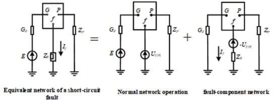
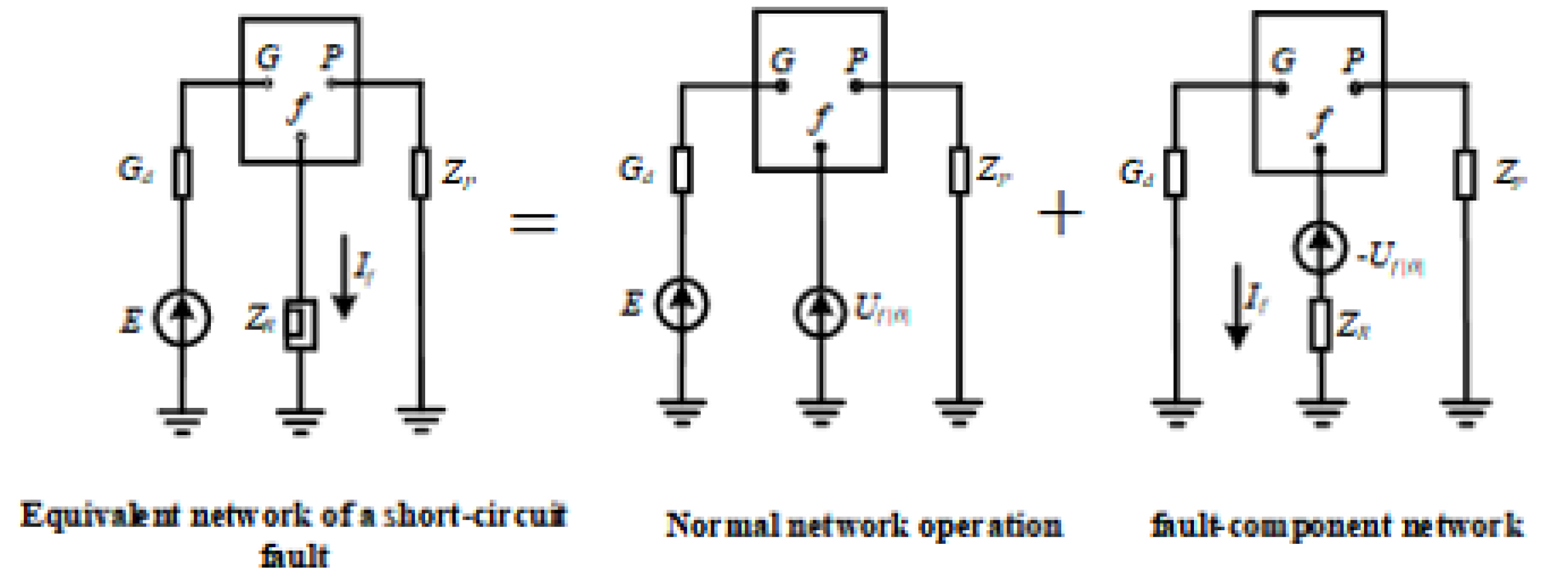
When a short-circuit fault happens in a power system, the current becomes concentrated around the fault point. At the same time, distributed energy resources keep injecting current into the system. As a result, branches closer to the fault location usually carry larger current amplitudes [15]. According to the superposition theorem, the post-fault system can be seen as the sum of the normal steady-state network and a pure fault-component network. The fault-component network can be further treated as a fault current source injected at the short-circuit point [19,20]. Based on the above analysis, the equivalent network of a short-circuit fault is built, as shown in Figure 1. The analysis is conducted using a linearized symmetrical-component model under a fixed prefault operating condition. The network topology and passive parameters are assumed constant within the short fault interval, and converter-interfaced sources are represented by local linear equivalents. These assumptions limit the derivation to the considered operating condition and do not represent general nonlinear dynamics.

Figure 1. Equivalent circuit for short-circuit fault analysis.

In Figure 1, G denotes the generator node, P the load node, and f the fault node. G_d and E are the generator transient reactance and equivalent electromotive force, respectively, and Z_P is the equivalent load impedance. Z_f denotes the additional fault-branch impedance for an asymmetrical short circuit and the grounding resistance for a three-phase short circuit. U_f(0) is the prefault voltage phasor at the fault point, and I_f is the fault current. Assuming n nodes and l directed branches in the fault network, the following relationship holds:

$$\Delta U=Z\Delta I=Y^{-1}\Delta I$$

(1)

where ΔU is the vector of node-voltage fault components, Z is the node-impedance matrix, Y is the node-admittance matrix, and ΔI is the current-injection fault-component vector whose only nonzero entry is the fault current at node f. Therefore, the following relationship is obtained:

$${\dot{I}}_f={\displaystyle \frac{{\dot{U}}_{f|0|}}{Z_{ff}+Z_{\Delta }}}$$

(2)

$$\left[\begin{array}{c}\Delta {\dot{U}}_1\\ ⋮\\ \Delta {\dot{U}}_f\\ ⋮\\ \Delta {\dot{U}}_n\end{array}\right]=-{\dot{I}}_f\left[\begin{array}{c}{Z}_{1f}\\ ⋮\\ Z_{ff}\\ ⋮\\ Z_{nf}\end{array}\right]$$

(3)

From the above equation, it can be seen that the ratios ${\Delta U}_i^{\mathit{\&}}/\Delta U_k^{\mathit{\&}}$ between the voltage fault components of different nodes are only related to the elements in the f-th column of the Z matrix. Therefore, it can be concluded that the voltage fault components of different nodes do not depend on the short-circuit type. Since node voltages are less distinguishable than branch currents, the branch current in the fault-component network can be written as:

$$\Delta I_b=(Y_{b}A+Y_{b0}{A}_0)\Delta U$$

(4)

In Equation (4), ΔI_b is the branch-current fault-component vector, Y_b is the branch-admittance matrix, A is the branch-to-node incidence matrix, Y_b0 is the sending-end shunt-admittance matrix, and A₀ is the corresponding node-incidence matrix.

The short-circuit fault network model above can represent both two-phase and three-phase short-circuit faults. Because two-phase short-circuit faults are asymmetrical, their fault characteristic component is the negative-sequence current [20]. For three-phase short-circuit faults, the fault characteristic component is the positive-sequence current [20]. However, when a three-phase short-circuit fault happens, the node voltage quickly drops to 0. At the same time, the system frequency also decreases.

Common short-circuit faults in power systems also include ungrounded faults. Because of the ungrounded fault characteristics, the fault current path and sequence components change when this type of fault occurs. An ungrounded short-circuit fault changes the boundary condition at the fault point. This means the injection pattern of the ∆I vector in Equation (1) changes, and the specific value of ∆I also changes. However, the proportional relationship in Equation (4) stays unchanged. This relationship is decided by the network topology and parameters. In a two-phase ungrounded fault, the currents in the two faulted phases have the same size but opposite directions. There is no current in the unfaulted phase. In a three-phase ungrounded fault, the three phases stay symmetrical. The current magnitude is large, and the voltage drops greatly. Similarly, there is no zero-sequence component. A decrease in system frequency is also seen.

2.2. Mechanism Analysis of Branch Open-Circuit Disturbances

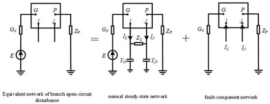
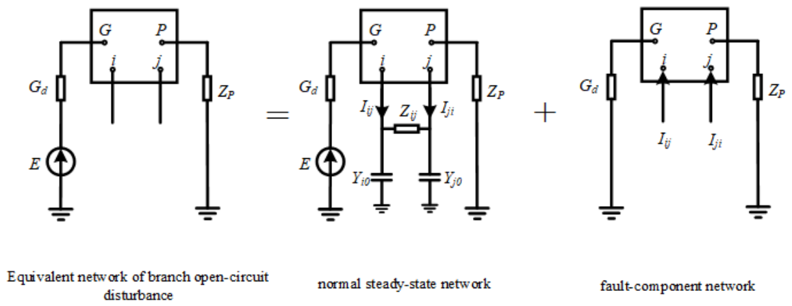
Branch open-circuit disturbance is an important factor that causes sudden changes in power grid operation mode. Since an open circuit does not have obvious electrical fault features, it is harder to detect and identify. In terms of topology, a branch open circuit can be seen as disconnection at both sides of the branch, or disconnection at only one side. Figure 2 shows the equivalent network model when a two-side open circuit happens on the directed branch for the case where only the i side is disconnected, the analysis method is similar to the two-side open circuit case. The difference is that an equivalent virtual node needs to be added at the open-circuit point. The rest of the modeling and analysis steps stay the same [20].

Figure 2. Equivalent circuit for branch open-circuit analysis.

In Figure 2, I_ij and I_ji denote the current phasors through the directed branches ij and ji under normal operation, consistent with the labels used in the figure. Y_i0 and Y_j0 are the admittance-to-ground matrices at the two ends of branch ij. The remaining symbols have the same meanings as in Figure 1. Because a branch open circuit disconnects the two ends of the branch, the current sources in the fault-component network have the same magnitudes as the prefault branch currents but opposite directions.

$$\Delta I_b=(Y_{b}A+Y_{b0}{A}_0)Y^{-1}\Delta I$$

(5)

Because a branch open circuit changes the network topology, Y, Y_b, Y_b0, and A₀ in Equation (5) are formed after removing the disconnected branch. When both ends of branch ij are open, the entries in rows i and j of the injection vector are I_ij and I_ji, respectively; all other entries are zero.

$$I_b=I_{b|0|}+\Delta I_b$$

(6)

3. Power System Fault Data Acquisition Based on Compressed Sensing

3.1. Sparse Signal Representation Model Based on Compressed Sensing

Sparse signal representation is a method used to approximate the original signal, and it represents the signal by a linear combination of several atoms. In this process, the number of selected atoms is much smaller than the dimension of the signal, so the main features of the signal can be extracted in an effective way. The dictionary is an important basis of sparse representation. The fault mechanism analysis in Section 2 gives a theoretical basis for constructing a suitable and efficient dictionary. In this paper, an Online Dictionary Learning (ODL) method is used [10]. This method updates the dictionary online through a recursive process, and mini-batch samples are processed step by step. In this way, the dictionary can better adapt to the dynamic characteristics of the system and represent them more flexibly [10]. In the implemented single-channel case, each normalized window is $y\in R^{100}$, the overcomplete dictionary is $D\in R^{\left(100\times 200\right)}$, and the sparse coefficient vector is $x\in R^{200}$; in general, $y\in R^m$, $D\in R^{\left(m\times K\right)}$, and $x\in R^K$ with $K>m$.

Given signal $y\in R^m$ and overcomplete dictionary $D\in R^{m\times k}(k>m)$, sparse representation is used to find a set of sparse coefficients $x\in R^k$. Based on these sparse coefficients, the original signal can be represented as $y=Dx$. At the same time, the number of nonzero elements in x needs to be reduced as much as possible, that is, ||x||₀ should be made as small as possible. Here, ||x||₀ denotes the L₀ norm of x. The minimization of this norm is a combinatorial optimization problem, and this kind of problem is difficult to solve directly. For this reason, the L₁ norm is usually used to replace the L₀ norm in practical calculation. In this case, the problem of finding the optimal sparse representation can be transformed into Equation (7), where $\lambda >0$ is the regularization parameter. This parameter is used to balance the reconstruction error and the sparsity of the solution [11].

$$\widehat{x}=\underset{x}{min}{\displaystyle \frac{1}{2}}||y-Dx|{|}_2^2+\lambda ||x|{|}_1$$

(7)

In the ODL process, the dictionary $D$ is learned from the available training signals. In this work, high-resolution point-on-wave electrical signals obtained from PSCAD/EMTDC are used for dictionary training. For real-world applications, the required waveform data should be provided by DFRs or waveform-capable measurement devices, since standard synchrophasor measurements cannot provide the required temporal resolution.

$$V=\underset{D,X}{min}||Y-DX|{|}_2^2$$

(8)

where $X=[x_1,x_2,\cdots ,x_n]$ is the sparse coefficient matrix. The optimization model can be solved by using an alternating optimization strategy. In this process, the dictionary D is fixed first, and the sparse coefficient matrix X is optimized under this condition. Then, X is fixed, and D is optimized again, so that the dictionary can be updated step by step.

3.2. Principle of Online Dictionary Learning

The objective of the online dictionary learning method can be expressed as a stochastic optimization problem [10]. The main idea of this method is to update the dictionary step by step when new samples are input. Through this updating process, the expected loss function can be reduced as much as possible. Therefore, this problem can be further transformed into solving Equation (9):

$$L=\underset{D\in C}{min}{\displaystyle \frac{1}{T}}{\sum }_{t=1}^T(\underset{x_t\in R^k}{min}{\displaystyle \frac{1}{2}}{‖y_t-D{x}_t‖}_2^2+\lambda {‖x_t‖}_1)$$

(9)

where T denotes the total number of samples; $y_t\in R^m$ denotes the t-th data sample; $D=[d_1,d_2,\dots ,d_k]\in R^{m\times k}$ denotes the dictionary that needs to be learned, and each column vector dj is an atom in the dictionary; $x_t\in R^k$ is a sparse vector, and it represents the sparse coding corresponding to yt. $C$ is the constraint set of the dictionary, and it satisfies expression $C=\{D\in R^{m\times k}|\hspace{0.33em}{‖d_j‖}_2\le 1,\forall j\}$. This constraint is used to limit the sparsity of the elements in the dictionary. The main idea of online dictionary learning is not to directly solve the batch optimization problem based on all samples. Instead, the dictionary is updated one by one when new samples are input, and this process is carried out by using a stochastic approximation strategy. Based on this idea, the online dictionary learning method proposed in this paper divides the above problem into two alternating steps, namely sparse coding and dictionary updating.

For the sample y_t at time t, the dictionary D_t−1 obtained from the previous time instant is given first. Under this condition, the sparse representation x_t of y_t can be calculated, namely:

$$x_t=\mathit{arg}\underset{x}{min}({\displaystyle \frac{1}{2}}{‖y_t-D_{t-1}x‖}_2^2+\lambda {‖x‖}_1)$$

(10)

In the updating process, the proposed method uses two intermediate statistical quantities, A_t and B_t, to collect the historical information of the data. After these statistical quantities are obtained, the dictionary D_t is updated based on them. The expressions of the two intermediate statistical quantities are given as follows:

$$\begin{array}{c}{A}_t=A_{t-1}+x_t{x}_t^T\\ B_t=B_{t-1}+y_t{x}_t^T\end{array}$$

(11)

where $A_t\in R^{k\times k}$ denotes the expectation of the autocorrelation matrix of the sparse coefficients, and $B_t\in R^{m\times k}$ denotes the expectation of the cross-correlation matrix between the original signal and the sparse coefficients. Based on the accumulated statistical quantities obtained at the intermediate time instant, the dictionary D_t is updated and solved. This process can be expressed as:

$$D_t=\mathit{arg}\underset{D\in C}{min}{\displaystyle \frac{1}{t}}({\displaystyle \frac{1}{2}}Tr(D^{T}D{A}_t)-Tr(D^T{B}_t))$$

(12)

Based on the sparse coefficient x_t of the sample, the dictionary D_t is updated. In this step, block coordinate descent is often used. In this method, the dictionary atoms d_j are updated one column after another, while the other columns remain fixed. This updating way is used to make the dictionary satisfy the unit-norm constraint. For the j-th atom d_j, the update formula is given by:

$$u_j={\displaystyle \frac{{B_t}_j-D{A_t}_j}{{A_t}_{jj}}}+d_j$$

(13)

where $A_{tjj}$ [j,j] is the j-th diagonal element of A_t; $A_{tj}$ and $B_{tj}$ denote the j-th column elements of A_t and B_t, respectively. After u_j is updated, the updated atom u_j needs to be projected. This step is used to make sure that the updated atom can satisfy the unit-norm constraint:

$$d_j={\displaystyle \frac{u_j}{\mathit{max}({‖u_j‖}_2,1)}}$$

(14)

In the implementation, the waveform sampling frequency is set to 20 kHz, with a 100-point window (5 ms) and a 20-point sliding interval (1 ms). The dictionary size is configured as $100\times 200$, and OMP is adopted for sparse coding with a maximum of 15 selected atoms and a residual threshold of ${10}^{-6}$. A coefficient is regarded as active when its magnitude is larger than ${10}^{-3}$. Although Equation (9) describes the general ${\mathcal{l}}_1$-based ODL formulation, the practical sparse coding process in this work is governed by the OMP stopping rules, including the maximum support number and residual error.

4. Power System Fault-Type Identification Method Based on an STP–Attention Spiking Neural Network

4.1. STP–Attention Spiking Neural Network Method

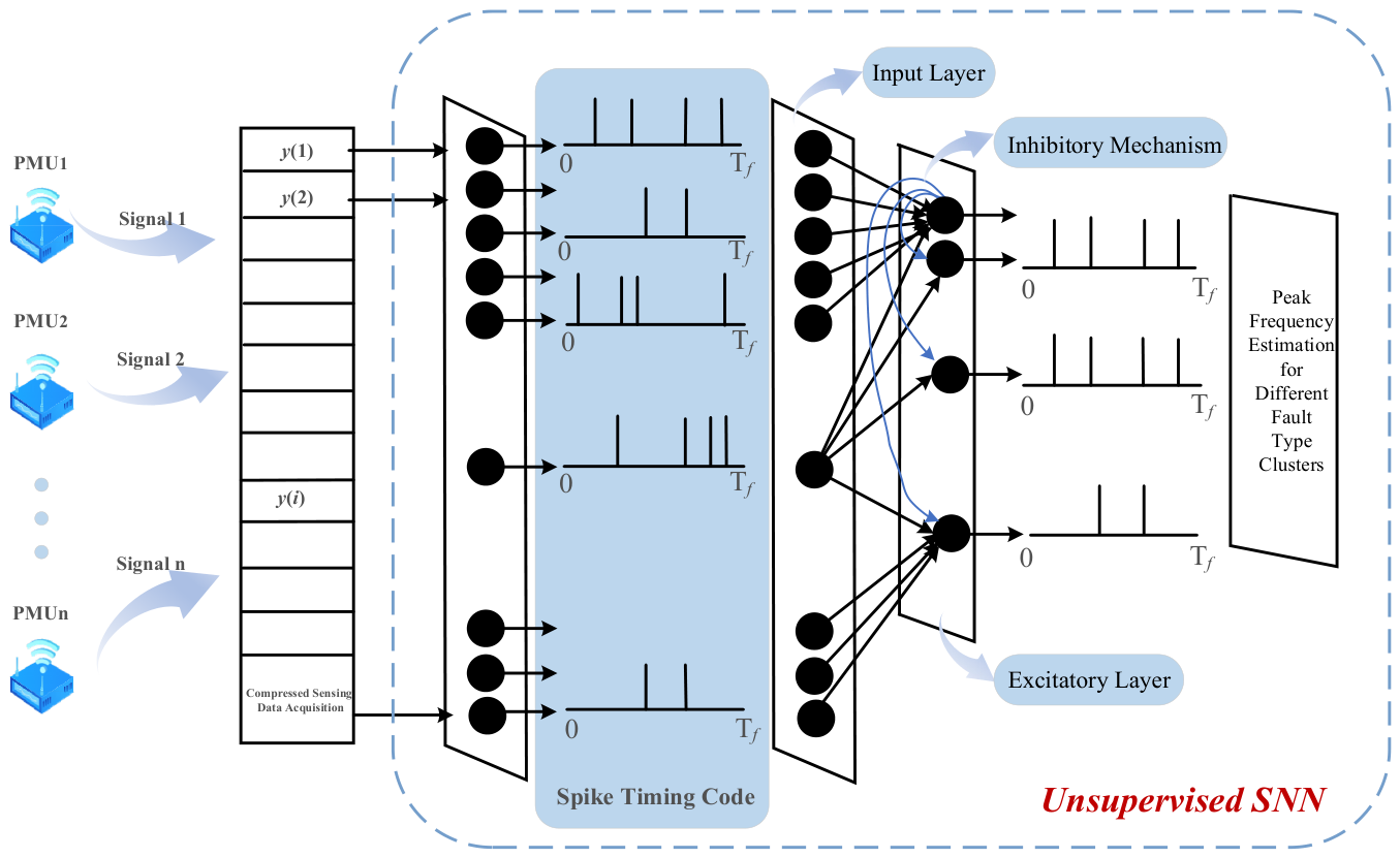
The unsupervised spiking neural network uses a two-tier architecture, which includes an input layer and an excitatory layer. The number of neurons in the input layer is decided by the number of signal channels. Each input neuron is fully connected with the neurons in the excitatory layer through synapses. The network uses spike-timing-dependent plasticity to adjust the synaptic weights by itself according to the firing time of spikes. In this way, neural activities with temporal correlation can be strengthened [12]. In the excitatory layer, lateral inhibition and a homeostatic mechanism are used together. These two mechanisms make neurons compete with each other, and they also guide different neurons to learn different features from the input data. Through this competitive process, the network can gradually produce selective responses to different sample patterns and distinguish these patterns more clearly.

The input layer first encodes the sampled data into spike trains, and then sends these spike trains to the excitatory layer. After the neurons in the excitatory layer receive the incoming spikes, they generate synaptic responses. When an input spike reaches the neuron at time t_c, its value is set to 1, which means that a spike exists at this moment. The excitatory postsynaptic potential (EPSP) caused by this input spike lasts from t_c to t_d, and it can affect the membrane potential of the postsynaptic neuron during this time interval. This time interval also represents the effective time in which a single input spike can influence the following neurons. Within this period, the EPSP value is set to 1. The above process can be described as follows:

$$EPSP(t)=\left\{\begin{array}{cc}1& t_c\le t\le t_d,s(t_c)=1\\ 0& otherwise\end{array}\right.$$

(15)

In Equation (15), $t_c$ denotes the arrival time of a presynaptic spike and $t_d$ represents the end of its effective postsynaptic potential interval. Both time instants are determined by the spike timing and the configured EPSP duration, rather than the fault class.

The membrane potential dynamics of the leaky integrate-and-fire (LIF) neurons in the excitatory layer are described by Equation (16). This equation shows how the membrane potential changes over time when the neuron receives excitatory postsynaptic potential (EPSP) inputs:

$${\tau }_{mt}{\displaystyle \frac{d{u}_p(t)}{dt}}=-u_p(t)+\omega (t){\sum }_{T_f}EPSP(t)-I$$

(16)

Here, ${\tau }_{mt}$ denotes the membrane time constant, and it is used to control the decay rate of the membrane potential $u_p(t)$ toward the resting potential when there is no external input. A larger ${\tau }_{mt}$ means that the decay process becomes slower. $u_p(t)$ represents the membrane potential of the neuron at time t. $\omega (t)$ denotes the synaptic weight at time t. $T_f$ is the set of all spike times $t_f$ in the input spike train. I represents the external inhibitory current, and it is a constant value. This current has a global inhibitory effect on the neuronal membrane potential.

When $u_p(t)$ reaches the firing threshold, the neuron generates a spike. After the spike is generated, its membrane potential $u_{th}(t)$ is reset, and the postsynaptic neurons are also affected to fire at the same time. After this spiking event, the neuron enters a refractory period. During this period, $u_p(t)$ remains unchanged. In addition, a homeostatic mechanism is added to the system, so that one neuron will not become too active and dominate the whole response. In this mechanism, after each discharge, the firing threshold $u_{th}(t)$ of the spiking neuron is increased according to ${\theta }_r$. This process can be expressed by the following equation:

$$u_{th}=(1+{\theta }_r)u_{th}$$

(17)

In this framework, a bio-inspired unsupervised learning mechanism based on spike-timing-dependent plasticity (STDP) is proposed. In the learning phase, the synaptic weights are updated only when postsynaptic spikes arrive. The main idea of STDP is to adjust synaptic weights according to the temporal correlation between pre- and postsynaptic spike events. For each connection between the input layer and the excitatory layer, the STDP weight update rule is given as follows [12]:

$$\Delta \omega =\left\{\begin{array}{cc}{\epsilon }_1{e}^{(-\Delta t/{\tau }_1)},& \Delta t>0\\ {\epsilon }_2{e}^{(-\Delta t/{\tau }_2)},& \Delta t<0\end{array}\right.$$

(18)

where $\Delta t=t_{post}-t_{pre}$ is the time difference between the postsynaptic and presynaptic spikes; $t_{pre}$ and $t_{post}$ denote their respective firing times; and ${\epsilon }_1,{\epsilon }_2,{\tau }_1,$ and ${\tau }_2$ are the constants used for weight updating. The relation defining $\Delta t$ is explanatory text rather than a separately numbered approximation.

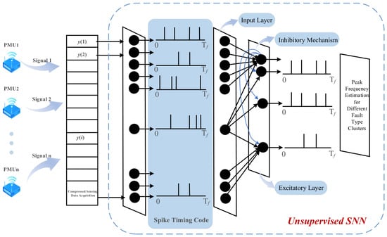
In summary, the unsupervised spiking neural network uses a two-layer architecture, which consists of an input layer and an excitatory layer. Signal transmission between the two layers is completed through fully connected synapses. The network uses the spike-timing-dependent plasticity rule to adjust synaptic weights by itself according to the firing order of spikes, and this process makes unsupervised learning possible. In the excitatory layer, lateral inhibition and a homeostatic mechanism are also introduced. These mechanisms make neurons compete with each other and learn different feature patterns from the input data. Finally, different neurons can form specialized responses to specific input categories. The typical architecture of the network is shown in Figure 3. Related research has also demonstrated the applicability of spiking neural networks in power system disturbance and fault diagnosis tasks [8,9]. After STDP training, the synaptic weights are fixed and labeled samples are used for neuron–class assignment. The ten excitatory neurons producing the highest spike counts for each sample participate in the voting process, and each neuron is assigned to the class with the maximum accumulated votes. During inference, the classification result is obtained by aggregating the responses of neurons according to this mapping.

Figure 3. Architecture of the SNN-based fault classifier.

When a fault occurs in a power system, the transient fault signals usually show non-stationary, strongly nonlinear, and time-varying characteristics. As mentioned above, sparse representation based on compressed sensing theory can reduce the dimension of data effectively, and it can also realize efficient data extraction. However, when conventional spiking neural network (SNN) neurons are used to process these signals, there are still two main limitations. First, static synaptic weights cannot describe the rapid decay patterns of high-frequency oscillations during faults. Second, in the classification stage, the neurons respond to all input spikes in the same way, and they do not have enough selectivity for the key feature components used to distinguish different fault types. To solve these problems, this paper introduces short-term plasticity (STP) and an attention mechanism into the leaky integrate-and-fire neuron framework. STP provides temporal adaptive ability, and the attention mechanism provides weight allocation ability. Based on these two parts, a new neuron model is constructed. This model has both temporal dynamic adaptability and feature selectivity. The improved model is used to extract important temporal patterns from power system fault signatures, and it can also reduce the influence of noise interference. Related research has also demonstrated the applicability of spiking neural networks in power system disturbance and fault diagnosis tasks [8,9].

Short-term plasticity (STP) is a fast adaptive mechanism at the synaptic level [13]. It can dynamically adjust the response strength of synapses according to the recent input history, so the temporal information can be encoded quickly. STP mainly includes two forms, namely short-term facilitation (STF) and short-term depression (STD). Short-term facilitation (STF) means that the synaptic efficacy is temporarily enhanced under high-frequency spike stimulation. Short-term depression (STD) means that the synaptic efficacy is temporarily reduced after continuous activity. For a presynaptic neuron i and a postsynaptic neuron j, the synaptic efficacy $g_{ij}\left(t\right)$ consists of a static weight and a dynamic component $f_{ij}\left(t\right.$). It can be expressed as follows:

$$g_{ij}(t)={\omega }_{ij}+f_{ij}(t)$$

(19)

The dynamic component is regulated by spike inputs and synaptic plasticity parameters. The proposed model updates the internal dynamic state based on spike-driven activity and predefined synaptic rules. The formulation of this update process is given in Equation (20):

$${\tau }_{STP}{\displaystyle \frac{d{f}_{ij}(t)}{dt}}=-f_{ij}(t)+{\gamma }_{ij}{p}_i(t)h_j(t)$$

(20)

Here, ${\tau }_{STP}$ is the STP time constant, and it is used to control the decay rate of the dynamic component. ${\gamma }_{ij}$ is the learning rate parameter, and it adjusts the strength of Hebbian plasticity. $p_i\left(t\right)$ denotes the presynaptic spike input, and $h_j\left(t\right)$ represents the state of the postsynaptic neuron.

The introduction of STP allows neurons to adjust their response intensity dynamically according to the history of incoming spikes. STF is more suitable for capturing sudden fault events, such as current surges in post-fault transient processes. STD can reduce neuronal saturation by suppressing sustained activity, and this helps the model handle persistent faults in a more balanced way. To further improve the selectivity of neurons for sparse fault features, this paper adds an attention mechanism [14] to the sparse coefficients extracted by compressed sensing. By calculating the importance weights of different coefficients, the model can focus on the key feature components in an adaptive way. Specifically, the attention weight $a_i$ is obtained by normalizing the absolute values of the sparse coefficients $x_i$, as follows:

$$a_{\mathrm{i}}={\left|x_{\mathrm{i}}\right|}^{\mathsf{\beta }}/{{\mathsf{\Sigma }}_{\mathrm{j}=1}}^{\mathrm{K}}\left|x_{\mathrm{j}}\right|\mathsf{\beta }$$

(21)

Here, β > 0 controls the concentration of the attention weights. Values β > 1 emphasize a smaller number of dominant coefficients, whereas 0 < β < 1 produces a flatter distribution. The coefficient was set to β = 2 in all subsequent experiments. This value was selected from the grid β ∈ {0.5, 1, 2, 4} according to the validation results reported in Section 5.2.3.

The attention weights $a_i$ are combined with the STP-modulated synaptic efficacy, and then the final membrane potential integration equation is formed. In this equation, $u_j\left(t\right)$ denotes the state of the j-th neuron. The meanings of the other variables are the same as those defined in the preceding sections.

$${\tau }_m{\displaystyle \frac{d{u}_j(t)}{dt}}=-u_j(t)+{\sum }_i{a}_i{g}_{ij}(t)p_i(t)-I$$

(22)

By combining short-term plasticity with the attention mechanism, the neuron gets two kinds of adaptive abilities, one is at the temporal level and the other is at the feature level. At the temporal adaptation level, STP tracks the short-term temporal patterns of input spikes in an adaptive way, and this is done through the change in the dynamic component $f_{ij}\left(t\right)$, so the neuron becomes more sensitive to transient features like oscillation frequency and duration. At the feature adaptation level, the attention weights $a_i$ give different weights to the sparse coefficients in a dynamic manner, this helps the neuron focus on important feature components and suppress the less important or interfering ones, and in this way the feature distribution is selectively enhanced.

4.2. Implementation Workflow of the Improved SNN-Based Fault Classification Method

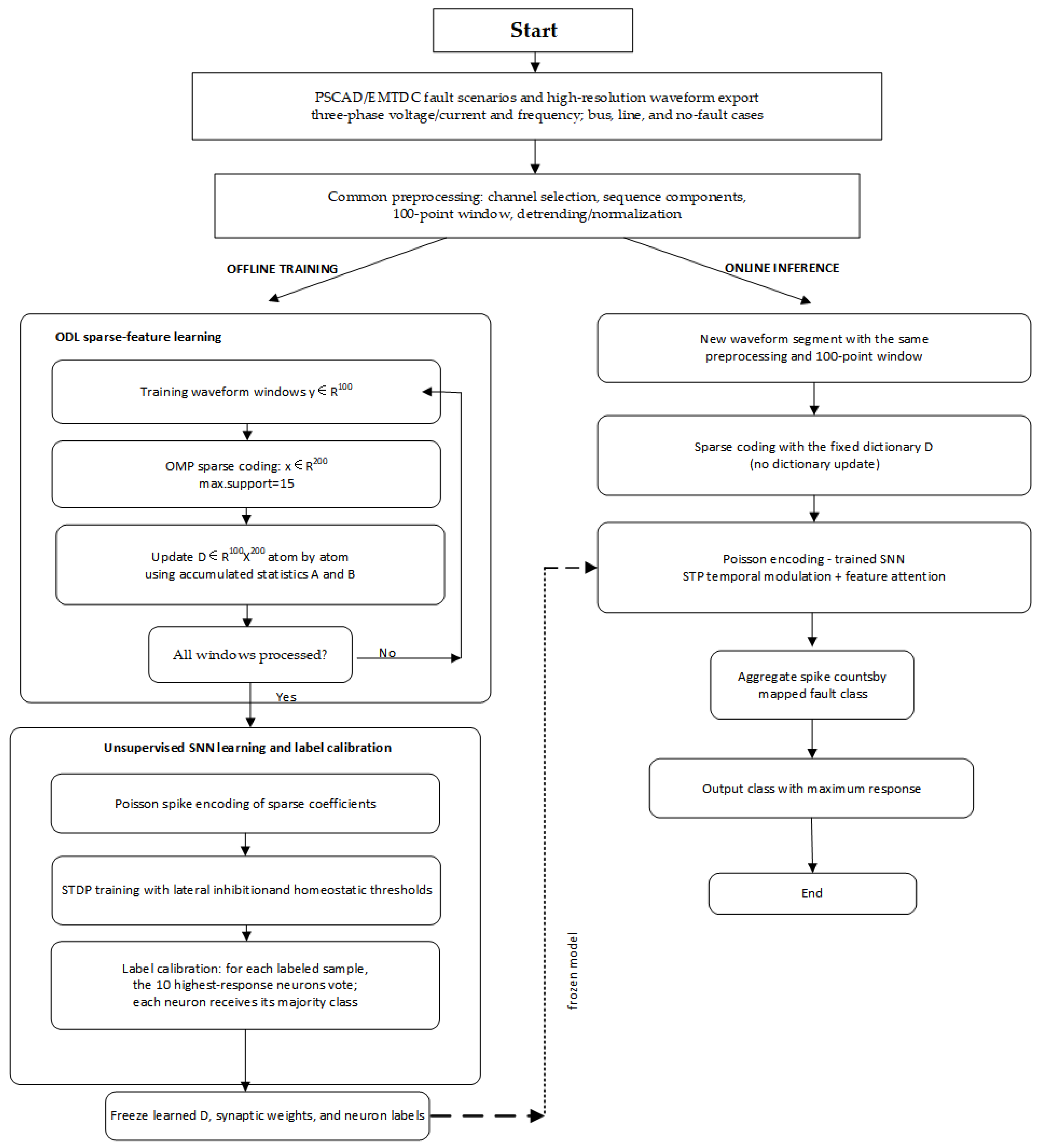
The fault dataset is generated in PSCAD/EMTDC, including bus faults, line faults, and no-fault cases. High-resolution three-phase voltage, current, and frequency point-on-wave signals are exported at a sampling frequency of 20 kHz. The obtained signals are then processed through channel selection, sequence-component decomposition, 100-point window segmentation, detrending, and normalization. For practical deployment, the required waveform inputs should be provided by DFRs or waveform-capable measurement units instead of conventional synchrophasor frames.

With the waveform sampling frequency set to 20 kHz, each 100-point window corresponds to 5 ms, and the sliding interval of 20 points represents 1 ms.

In the offline ODL stage, normalized training windows are used to obtain sparse codes through OMP and update the $100\times 200$ overcomplete dictionary. Each window is represented by a 200-dimensional sparse coefficient vector, with no more than 15 active coefficients.

The sparse coefficients are subsequently encoded into Poisson spike trains and used to train the excitatory SNN with STDP, lateral inhibition, and homeostatic regulation. After training, the dictionary and synaptic weights are fixed, and labeled samples are employed for neuron–class calibration according to the procedure described in Section 4.1.

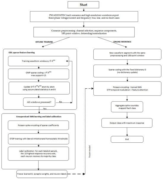
During inference, the same preprocessing procedure is applied to the input signals. Sparse coefficients obtained from the fixed dictionary are encoded and fed into the trained STP–attention SNN. The final fault category is determined according to the neuron–class mapping with the highest accumulated response. In the offline branch of Figure 4, the decision node asks whether all training windows have been processed: ‘No’ returns to sparse coding and dictionary updating, whereas ‘Yes’ proceeds to SNN learning and label calibration. The blocks in the online branch are processing operations and therefore do not introduce an additional decision branch.

Figure 4. Offline training and online inference workflow.

4.3. SNN Implementation Settings

Table 1 lists the fixed implementation settings used for numerical reproduction. The waveform sampling interval and the SNN integration step are different quantities: the former is 0.05 ms at 20 kHz, whereas the latter is 1 ms. The STDP and STP time constants follow commonly used ranges for event-driven unsupervised learning and dynamic synapses [12,13]. Five fixed random seeds were used to report the sensitivity statistics.

Table 1. Implementation settings of the ODL–STP–attention SNN.

Parameter	Value
Waveform sampling frequency	20 kHz
Window length/sliding step	100 points (5 ms)/20 points (1 ms)
Dictionary/sparse-code dimension	100 × 200/200
Maximum OMP support	15
Input channels	200
Excitatory/inhibitory neurons	600/600
SNN integration step/encoding duration	1 ms/100 ms
Resting/reset/firing threshold	−65/−65/−52 mV
Membrane time constant/refractory period	20/5 ms
STDP τ+/τ− and A+/A−	20/20 ms and 0.010/0.012
STP time constant/learning rate	200 ms/0.01
EPSP duration	5 ms
Attention coefficient β	2
Random seeds	11, 22, 33, 44, 55

5. Results and Discussion

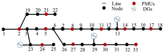
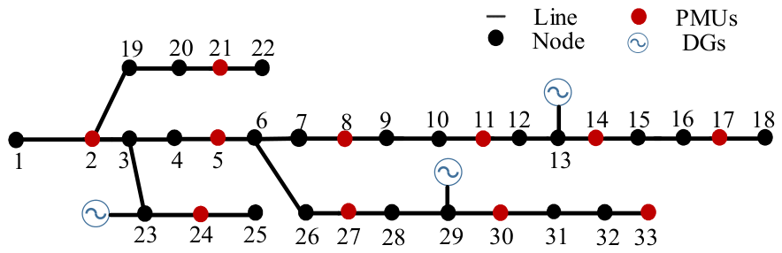
The electromagnetic transient system is modeled in PSCAD/EMTDC, where distributed-generation components, fault-switching events, and 20 kHz point-on-wave data are generated. MATLAB 2024a is used for subsequent processing, including signal preprocessing, ODL/OMP sparse representation, spike encoding, STDP-based training, neuron calibration, STP–attention inference, and evaluation. The PMU symbols in Figure 3 and Figure 5 only represent conceptual measurement locations and do not indicate standard synchrophasor measurements for acquiring high-resolution waveform data.

Figure 5. IEEE 33-bus test system [19].

The evaluation dataset is generated in PSCAD/EMTDC, including two-phase, three-phase, phase-to-ground, branch open-circuit, and normal operating conditions. The high-resolution point-on-wave signals are collected at 20 kHz and processed using 100-point windows with a 20-point stride. Note that the value of 500 in Table 2 corresponds to the number of independent samples for each individual fault subtype, such as AB, instead of the total samples of grouped fault categories (e.g., AB/AC/BC).

Table 2. Test conditions and dataset composition.

Fault Type	Fault Location	Sample Size
AB/AC/BC	Bus/Line	500
ABC	Bus/Line	500
AG/BG/CG	Bus/Line	500
ABG/ACG/BCG	Bus/Line	500
ABCG	Bus/Line	500
LF	Line	500
No Fault	-	500

In the table, AB stands for a two-phase short-circuit fault that happens on phases A and B, and AC and BC are defined in the same way. ABC is a three-phase short-circuit fault. AG is a single-phase-to-ground fault on phase A, while BG and CG are defined similarly. ABG means a two-phase-to-ground fault on phases A and B, and ACG and BCG are defined in the same manner. ABCG is a three-phase-to-ground fault. LF refers to a branch open-circuit fault.

5.1. Verification of Data Extraction via Compressed Sensing

5.1.1. Online Learning Dictionary

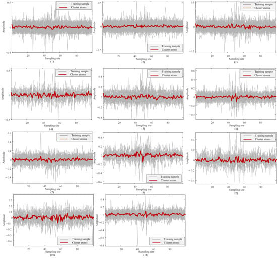
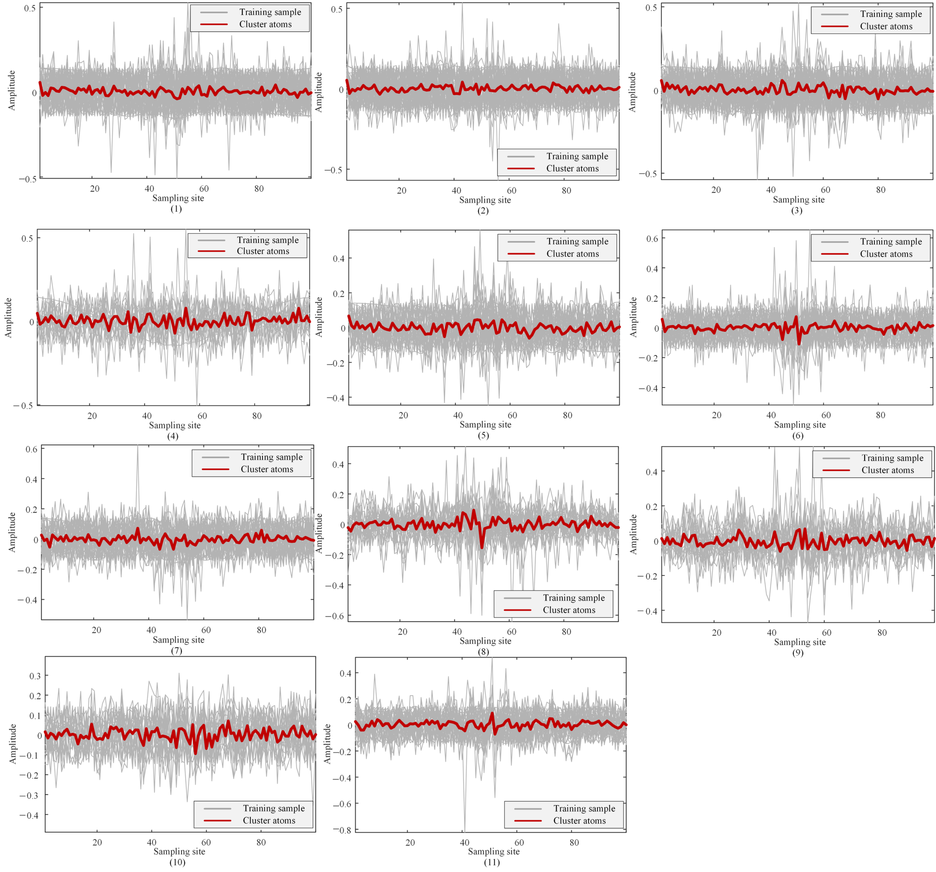
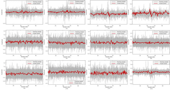
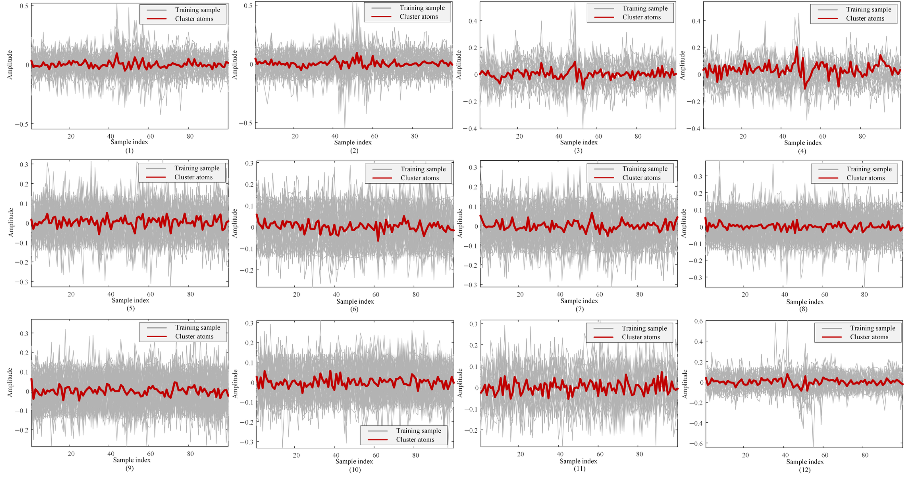
In this paper, a dataset is built from the fault data mentioned above, and this dataset is used to train the online learning dictionary. The dictionary atoms are updated through the online dictionary learning algorithm, so the dictionary can adapt to different fault types. The K-means clustering method is used to group the fault atoms, and the clustering results are shown in the figure below. More specifically, subfigures (1) to (11) in Figure 6 show the atom clusters for node faults. These clusters correspond to two-phase short-circuit faults (AB, AC, BC), three-phase short-circuit faults, single-phase-to-ground faults (AG, BG, CG), two-phase-to-ground faults (ABG, ACG, BCG), and three-phase-to-ground faults. In Figure 6 and Figure 7, the horizontal axis denotes the sample index within each 100-point window, and the vertical axis denotes normalized amplitude.

Figure 6. Dictionary-atom clusters for bus faults.

Figure 7. Dictionary-atom clusters for line faults.

The atom clusters for line faults are shown in Figure 7. These line faults include two-phase short-circuit faults, three-phase short-circuit faults, single-phase-to-ground faults, two-phase-to-ground faults, three-phase-to-ground faults, and branch open-circuit faults (LF). They are presented in subfigures (1) through (12) in the same order as listed above.

Based on the atom clustering results given above, the average reconstruction errors, the average sparsity values, and the corresponding clustered atom results for different fault types are shown in Table 3 and Table 4. Table 3 presents the results for bus faults, whereas Table 4 reports the corresponding results for line faults. These results are provided separately for bus faults and line faults. The grounded-fault classes generally require fewer active atoms and give lower reconstruction errors, whereas multi-phase and line-open cases use broader supports, consistent with their more complex waveform structure.

Table 3. Dictionary-atom clustering results for bus faults.

Fault Type	Average Reconstruction Error (%)	Average Sparsity (Atoms)	Cluster Index
AB	4.2	10.2	1
AC	4.5	10.5	2
BC	4.9	10.8	3
ABC	4.1	10.2	4
AG	2.7	8.3	5
BG	2.9	8.6	6
CG	2.6	8.5	7
ABG	3.2	9.5	8
ACG	3.3	9.7	9
BCG	3.1	9.2	10
ABCG	3.9	9.9	11

Table 3. Dictionary-atom clustering results for bus faults.

Fault Type	Average Reconstruction Error (%)	Average Sparsity (Atoms)	Cluster Index
AB	4.2	10.2	1
AC	4.5	10.5	2
BC	4.9	10.8	3
ABC	4.1	10.2	4
AG	2.7	8.3	5
BG	2.9	8.6	6
CG	2.6	8.5	7
ABG	3.2	9.5	8
ACG	3.3	9.7	9
BCG	3.1	9.2	10
ABCG	3.9	9.9	11

Table 4. Dictionary-atom clustering results for line faults.

Fault Type	Average Reconstruction Error (%)	Average Sparsity (Atoms)	Cluster Index
AB	4.5	10.4	1
AC	4.9	10.8	2
BC	5.0	11.1	3
ABC	4.5	10.5	4
AG	3.0	8.9	5
BG	3.2	9.1	6
CG	3.1	9.0	7
ABG	3.7	9.8	8
ACG	3.9	10.1	9
BCG	3.5	9.5	10
ABCG	4.3	10.6	11
LF	5.3	11.5	12

Table 4. Dictionary-atom clustering results for line faults.

Fault Type	Average Reconstruction Error (%)	Average Sparsity (Atoms)	Cluster Index
AB	4.5	10.4	1
AC	4.9	10.8	2
BC	5.0	11.1	3
ABC	4.5	10.5	4
AG	3.0	8.9	5
BG	3.2	9.1	6
CG	3.1	9.0	7
ABG	3.7	9.8	8
ACG	3.9	10.1	9
BCG	3.5	9.5	10
ABCG	4.3	10.6	11
LF	5.3	11.5	12

Here, average sparsity means the average number of dictionary atoms used to represent a signal in the sparse representation framework, and this value shows how complex the signal is and how well the dictionary works. When the sparsity is high, it means the signal patterns are more complex and need several atoms combined together to be represented accurately. When the sparsity is low, it means the signal patterns are simpler, and there are atoms in the dictionary that match them well, so the representation is more efficient. For the method proposed in this paper, the overall average reconstruction error for bus faults is 3.58%, and the average sparsity is 9.58. For line faults, these two values are 4.08% and 10.11, respectively. Specifically, for N samples, the average sparsity is ${\mathrm{S}}_{\mathrm{a}\mathrm{v}\mathrm{g}}=\left(1/\mathrm{N}\right){{\mathsf{\Sigma }}_{\mathrm{n}=1}}^{\mathrm{N}}\Vert {\mathrm{x}}_{\mathrm{n}}{\Vert }_0$, where a coefficient is counted as nonzero when $|{\mathrm{x}}_{\mathrm{n},\mathrm{k}}|>{10}^{-3}$ and ‖x_N‖₀ is limited to 15. The normalized reconstruction error is ${\mathrm{e}}_{\mathrm{a}\mathrm{v}\mathrm{g}}=(100/\mathrm{N}){{\mathsf{\Sigma }}_{\mathrm{n}=1}}^{\mathrm{N}}(\Vert {\mathrm{y}}_{\mathrm{n}}-\mathrm{D}{\mathrm{x}}_{\mathrm{n}}{\Vert }_2/\Vert {\mathrm{y}}_{\mathrm{n}}{\Vert }_2)$. No separate pass/fail threshold was imposed; the values below 6% are observed results rather than a preset acceptance criterion.

5.1.2. Data Acquisition via Compressed Sensing

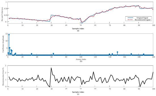
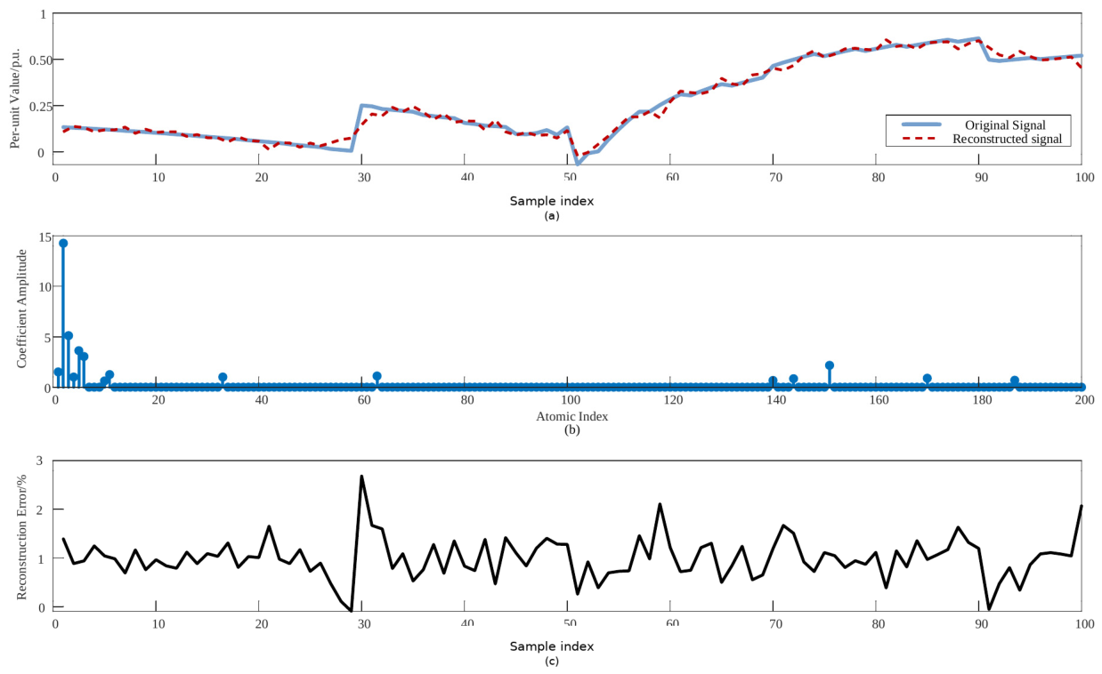
To check if the proposed online learning dictionary can adapt to different fault types, data are collected for the fault scenarios using both compressed sensing and the online learning dictionary. The AG fault set at Node 18 is taken as an example. The current signals after the fault are collected, and 100 sampling points are chosen to show the results. The reconstruction results of the fault signal are given in Figure 8. Figure 8a compares the original signal and the reconstructed signal. Figure 8b shows the sparse coefficients and the corresponding atom indices. Figure 8c presents the reconstruction error.

Figure 8. AG-fault signal reconstruction: (a) comparison between the original and reconstructed signals; (b) sparse coefficient amplitudes and the corresponding atom indices; (c) normalized reconstruction error.

For each fault subtype, 500 scenarios are generated and assigned to different locations in the IEEE 33-bus system. The continuous point-on-wave signals are segmented into 100-point windows using a 20-point stride, where each window contains 5 ms of waveform data. The horizontal axis in Figure 8 corresponds to consecutive sampling points within one waveform window and does not represent a reduction of 500 fault scenarios into 100 samples. The absolute fault-inception time from PSCAD is not displayed in this figure. To quantitatively evaluate the reconstruction performance across all fault categories, the reconstruction errors for bus faults and line faults are summarized in Table 5.

Table 5. Fault-signal reconstruction errors.

Fault Type	Node-Fault Reconstruction Error (%)	Line-Fault Reconstruction Error (%)
AB	4.79	4.93
AC	4.92	5.11
BC	4.88	5.02
ABC	4.39	4.88
AG	2.61	2.99
BG	2.68	3.06
CG	2.58	2.92
ABG	3.12	3.46
ACG	3.25	3.51
BCG	3.29	3.62
ABCG	4.08	4.18
LF	—	5.57

Table 5. Fault-signal reconstruction errors.

Fault Type	Node-Fault Reconstruction Error (%)	Line-Fault Reconstruction Error (%)
AB	4.79	4.93
AC	4.92	5.11
BC	4.88	5.02
ABC	4.39	4.88
AG	2.61	2.99
BG	2.68	3.06
CG	2.58	2.92
ABG	3.12	3.46
ACG	3.25	3.51
BCG	3.29	3.62
ABCG	4.08	4.18
LF	—	5.57

In summary, the online learning dictionary can adapt to different fault types by building a fault dataset and updating the dictionary atoms through clustering for each fault category. The compressed sensing reconstruction method proposed in this paper gives average reconstruction errors that are generally below 6% for the various fault scenarios set up in the IEEE 33-bus test system. This shows that the method is accurate and reliable for reconstructing fault signals in power systems. More specifically, the reconstruction errors for bus faults range from 2.58% to 4.92%, and for line faults they range from 2.92% to 5.57%.

5.2. Verification of Fault Type Identification in Power Systems

5.2.1. Fault Type Identification

The IEEE 33-bus fault dataset contains PSCAD-generated 20 kHz point-on-wave voltage, current, and frequency signals. Following sequence-component transformation and 100-point window segmentation, ODL/OMP is employed to extract 200-dimensional sparse representations. These representations are encoded into Poisson spike trains and input to the unsupervised SNN. Once STDP learning is completed, the synaptic weights are fixed, and neuron–class mapping is obtained using labeled calibration samples. The independent test set is then applied for performance evaluation.

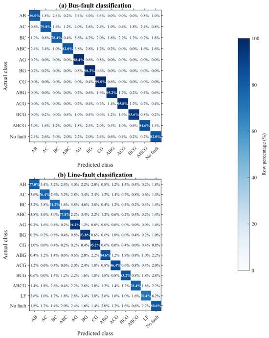
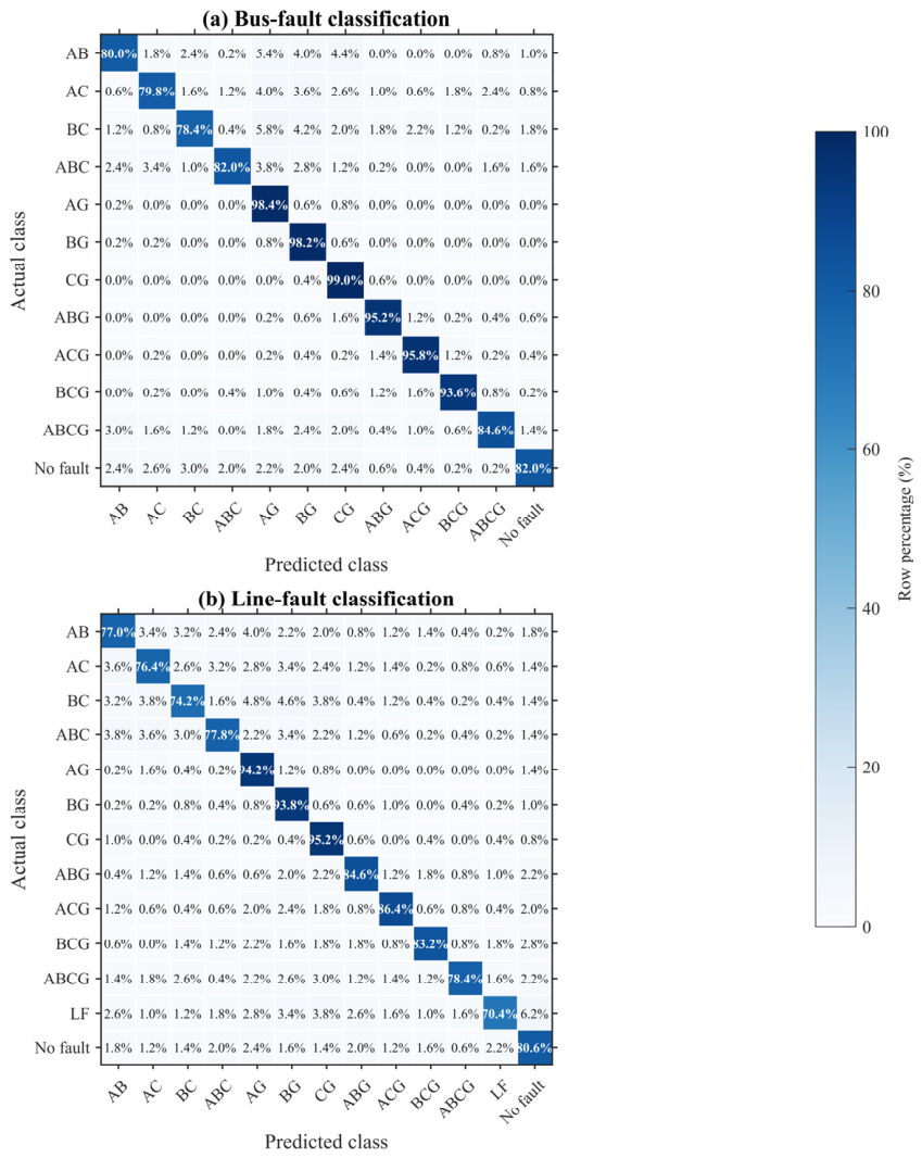
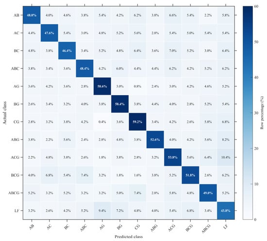
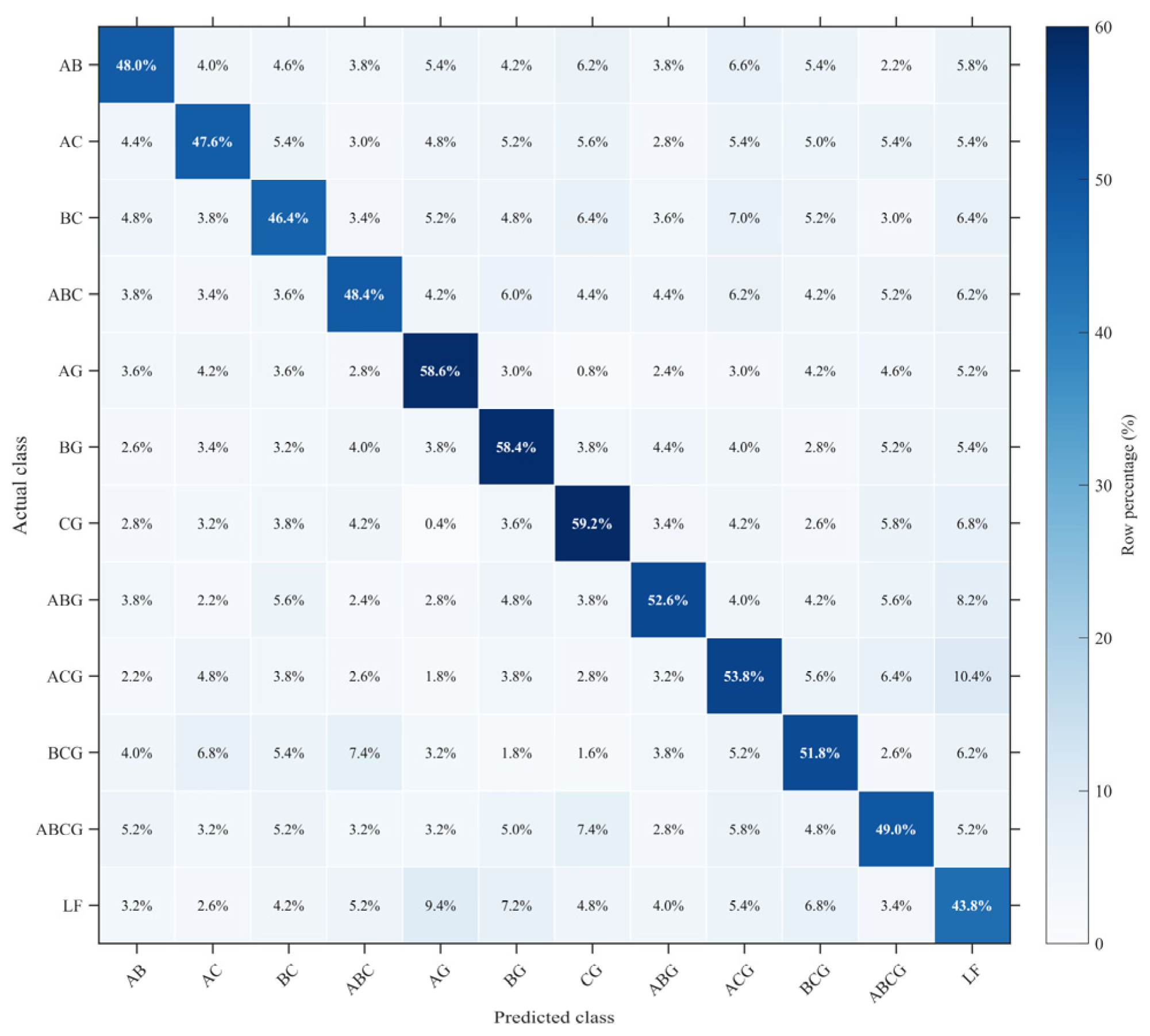
Figure 9 presents row-normalized confusion matrices, with every cell reported as a percentage of the corresponding actual-class row. The proposed method achieves classification accuracies of 88.93% for bus faults and 82.48% for line faults. The corresponding macro precision, recall, and F1-score are 89.40%, 88.94%, and 88.83% for bus faults and 82.99%, 82.48%, and 82.38% for line faults, respectively. Class-wise results are listed in Table 6 and Table 7.

Figure 9. Row-normalized confusion matrices for (a) bus faults and (b) line faults.

Table 6. Class-wise bus-fault classification metrics.

Fault Type	Precision (%)	Recall (%)	F1-Score (%)
AB	88.89	80.00	84.21
AC	88.08	79.80	83.74
BC	89.50	78.40	83.58
ABC	95.13	82.00	88.08
AG	79.61	98.40	88.01
BG	82.11	98.20	89.44
CG	84.33	99.00	91.08
ABG	92.97	95.20	94.07
ACG	93.19	95.80	94.48
BCG	94.74	93.60	94.16
ABCG	92.76	84.60	88.49
No fault	91.33	82.04	86.44
Macro average	89.40	88.94	88.83

Table 7. Class-wise line-fault classification metrics.

Fault Type	Baseline			20 dB SNR
	Precision (%)	Recall (%)	F1 (%)	Precision (%)	Recall (%)	F1 (%)
AB	79.38	77.00	78.17	54.30	48.00	50.96
AC	80.59	76.40	78.44	53.36	47.60	50.32
BC	79.78	74.20	76.89	48.84	46.40	47.59
ABC	84.20	77.80	80.87	53.54	48.40	50.84
AG	77.72	94.20	85.17	57.56	58.60	58.08
BG	76.51	93.80	84.28	54.17	58.40	56.21
CG	78.68	95.20	86.15	53.72	59.20	56.33
ABG	86.50	84.60	85.54	57.68	52.60	55.02
ACG	88.16	86.40	87.27	48.64	53.80	51.09
BCG	90.43	83.20	86.67	50.98	51.80	51.39
ABCG	91.59	78.40	84.48	49.60	49.00	49.30
LF	88.66	70.40	78.48	38.09	43.80	40.74
No fault	76.62	80.60	78.56	—	—	—
Macro average	82.99	82.48	82.38	51.71	51.47	51.49

5.2.2. Noise Impact

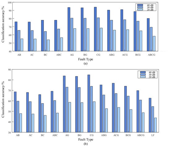
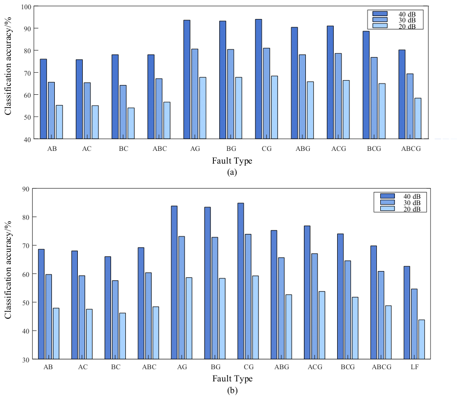
To investigate the noise robustness of the proposed method, Gaussian white noise with SNRs of 40, 30, and 20 dB is introduced into the continuous point-on-wave signals before window extraction. Figure 10 illustrates the corresponding classification accuracies for bus and line faults under different noise levels.

Figure 10. Classification accuracy under different SNRs: (a) bus-fault classification accuracy; (b) line-fault classification accuracy. The three bars for each fault type correspond to SNRs of 40, 30, and 20 dB, respectively.

As the SNR decreases, noise masks phase-dependent waveform features and perturbs the sparse representation, reducing classification accuracy. The degradation is more pronounced for line faults. The 20 dB results are therefore interpreted as a stringent window-based SNR stress test rather than evidence of field-ready protection performance. Section 5.3 further evaluates the time-resolved response during fault inception and clearing.

Figure 11 presents the row-normalized line-fault results at 20 dB SNR; each cell is expressed as a percentage and contrasting annotation colors are used to keep both diagonal and off-diagonal values legible. The overall accuracy is 51.47%, corresponding to 3088 correctly classified samples among 6000 test samples. Most errors occur between fault types with overlapping fault phases and neighboring line-fault signatures.

Figure 11. Row-normalized line-fault confusion matrix at 20 dB SNR.

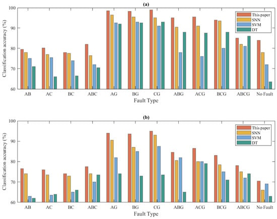
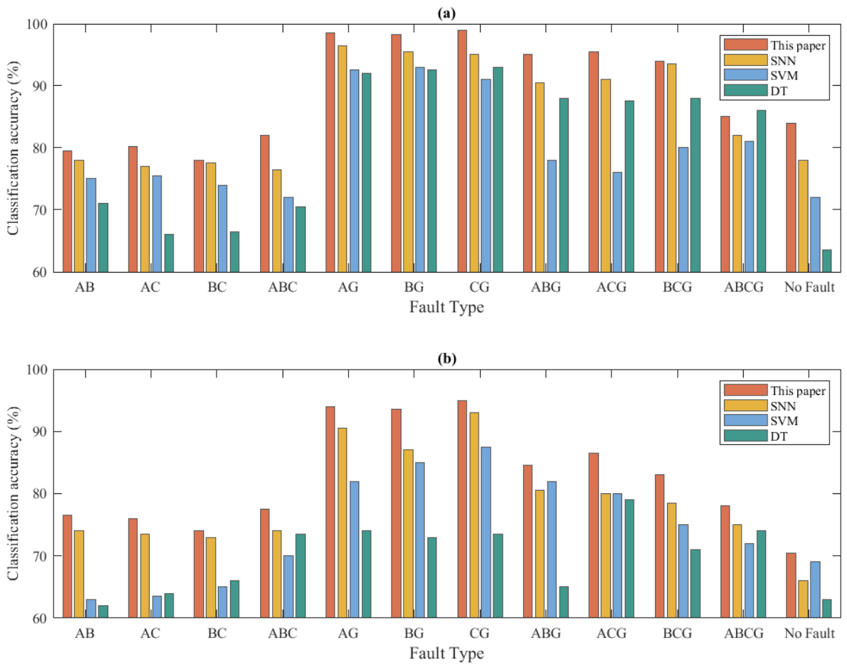
Figure 12 shows the performance comparison of the proposed method with SNN, SVM, and DT under the baseline condition. The enlarged figure improves the readability of the axes, legends, and class labels.

Figure 12. Comparison of classification accuracy among different algorithms under the baseline condition: (a) bus-fault classification; (b) line-fault classification.

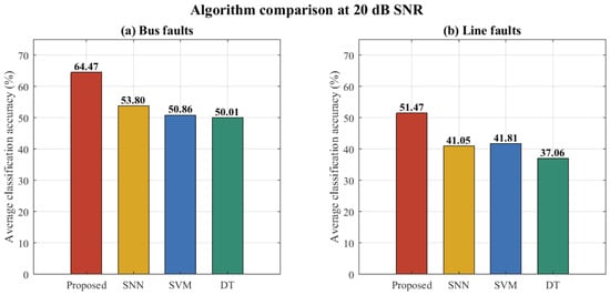
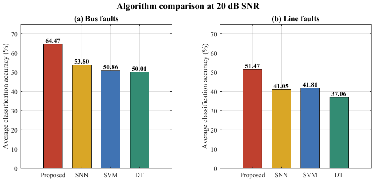
Figure 13 and Table 8 further present the average classification accuracies at 20 dB SNR based on the same test results. The reported line-fault accuracy is matched with the 20 dB confusion matrix result shown in Figure 11.

Figure 13. Average classification accuracy at 20 dB SNR.

Table 8. Classification accuracy at 20 dB SNR.

Case	Proposed (%)	SNN (%)	SVM (%)	DT (%)	Best Baseline (%)	Gain (Percentage Points)
Bus faults	64.47	53.80	50.86	50.01	53.80	10.67
Line faults	51.47	41.05	41.81	37.06	41.81	9.66

Under the 20 dB SNR condition, the proposed method achieves average classification accuracies of 64.47% for bus faults and 51.47% for line faults. The corresponding accuracies of SNN, SVM, and DT are 53.80%, 50.86%, and 50.01% for bus faults, and 41.05%, 41.81%, and 37.06% for line faults. The proposed method provides improvements of 10.67 and 9.66 percentage points over the best-performing baseline for bus and line faults, respectively.

The comparison indicates a relative advantage for the ODL–STP–attention SNN under the retained simulated conditions. Nevertheless, the substantial degradation of the aggregate line-fault accuracy at 20 dB shows that the method remains sensitive to severe measurement noise. The time-resolved case study in Section 5.3 is therefore used to examine response sequence and delay, rather than to claim field-ready protection performance.

5.2.3. Sensitivity to the Attention Coefficient β

The coefficient β determines how strongly the attention layer concentrates on dominant sparse coefficients. A five-run grid evaluation was conducted for β ∈ {0.5, 1, 2, 4}, while all other settings in Table 1 were held constant. The mean and standard deviation over the five fixed random seeds are reported in Table 9.

Table 9. Classification performance under different values of the attention coefficient β.

β	Bus-Fault Accuracy (%)	Line-Fault Accuracy (%)	Line-Fault Accuracy at 20 dB (%)
0.5	87.62 ± 0.41	81.31 ± 0.56	49.86 ± 0.74
1	88.24 ± 0.36	81.92 ± 0.48	50.73 ± 0.65
2	88.93 ± 0.29	82.48 ± 0.44	51.47 ± 0.61
4	88.51 ± 0.33	82.05 ± 0.51	50.92 ± 0.69

The results show a moderate optimum at β = 2. When β = 0.5, the attention distribution is relatively flat and weakly discriminative coefficients receive excessive weight. Increasing β to 2 improves all three indicators. A further increase to β = 4 slightly reduces accuracy because the attention becomes over-concentrated and suppresses complementary coefficients. Therefore, β = 2 is used in the remaining experiments.

5.3. Time-Resolved Transient Analysis Under Noisy Conditions

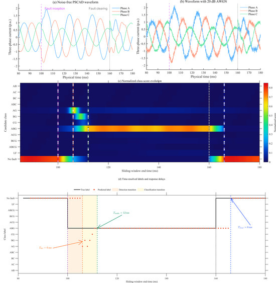
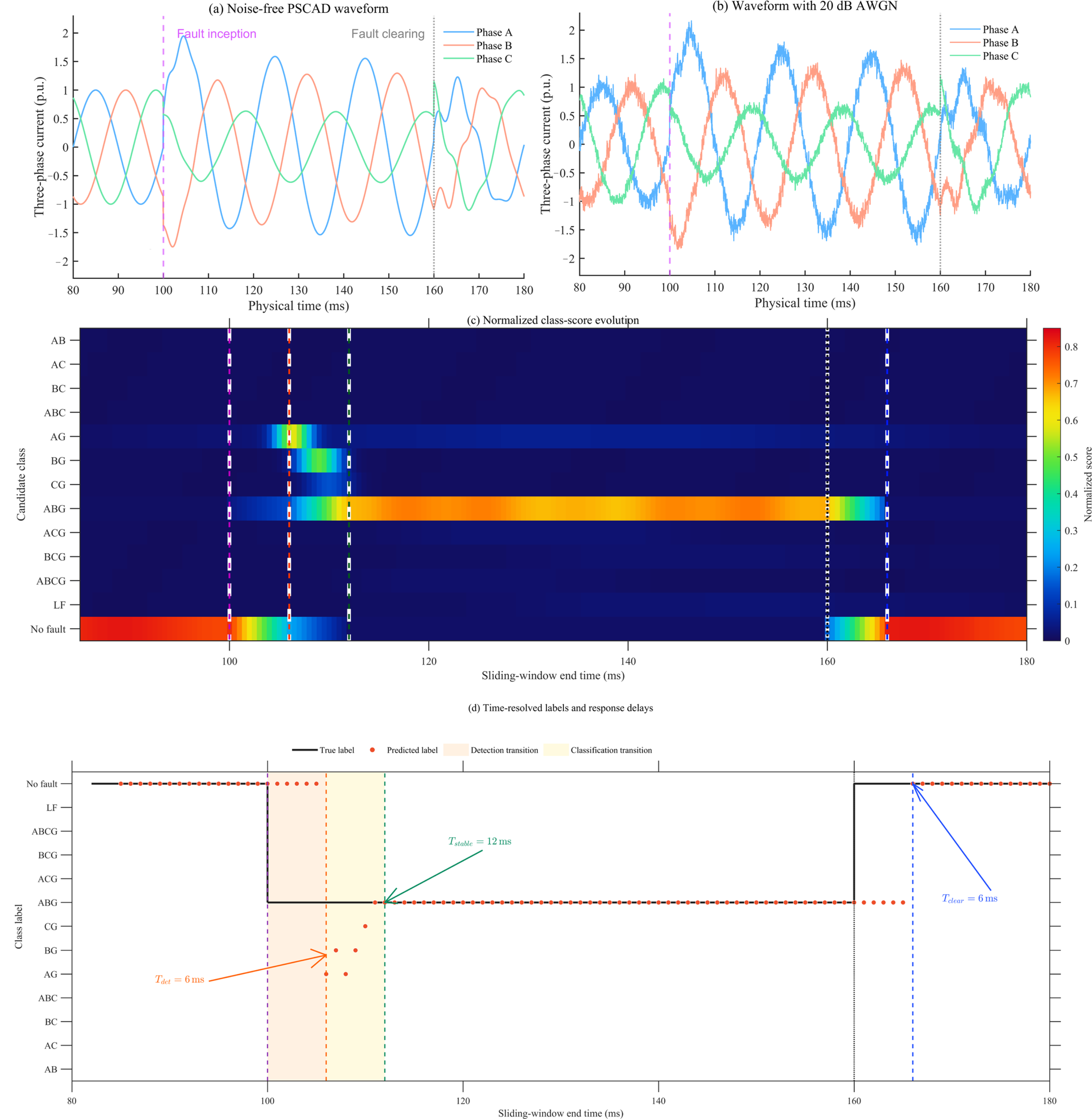
To complement the aggregate SNR results, a time-resolved numerical transient test was carried out using a parameterized three-phase point-on-wave current model. The sampling frequency was 20 kHz. An ABG fault was applied at 100 ms and cleared at 160 ms, and 20 dB additive white Gaussian noise was injected before window extraction. The continuous signal was processed by a 5 ms window with a 1 ms stride. For every window, the complete 13-class score vector and predicted label were retained. The numerical test used the fixed random seed. Figure 14 presents the noise-free waveform, the 20 dB waveform, the 13-class score sequence, and the corresponding predicted labels in panels (a–d), respectively.

Figure 14. Time-resolved response of an ABG fault under 20 dB SNR.

Three timing indices were calculated. Detection delay $T_{det}$ is the interval from fault inception to the first non-normal decision. Stable-classification delay $T_{stable}$ is the interval from fault inception to the first of five consecutive correctly classified ABG windows. Clearing-recovery delay $T_{clear}$ is the interval from fault clearing to the first of five consecutive no-fault decisions. These persistence criteria suppress isolated label changes caused by individual noisy windows.

As shown in Figure 14, the first persistent non-normal response occurs at 106 ms, giving T_det = 6 ms. During the following transition, the AG and BG scores increase because these classes share faulted phases with ABG. The ABG score becomes dominant and remains stable from 112 ms, corresponding to T_stable = 12 ms. After fault clearing, the output returns to the no-fault class at 166 ms, giving T_clear = 6 ms. The larger panels, fonts, and markers in Figure 14c,d are intended to make the class-score evolution and the three response-delay definitions directly readable.

6. Conclusions

Based on the modeling and detailed analysis of the mechanisms for various fault types, this paper gets an adaptive online learning dictionary that can handle multiple fault categories through an online learning strategy. With the help of compressed sensing theory, this dictionary can efficiently extract sparse features from different kinds of fault data. Finally, the improved spiking neural network is used to identify fault types quickly and accurately.

(1)

Starting from the underlying mechanisms, this work models and analyzes multiple typical faults, thereby overcoming the limitations of conventional purely data-driven approaches that are detached from physical backgrounds. This enhances the interpretability and reliability of the method and provides a theoretical basis for constructing fault features.

(2)

The proposed online adaptive dictionary learning method updates dictionary atoms in a dynamic way based on different fault characteristics, and this greatly improves the flexibility and accuracy of sparse representation. When combined with compressed sensing, this method not only extracts features from fault data efficiently while keeping good reconstruction accuracy, but also provides a solid data foundation for later sparsity-based applications like fault localization.

(3)

At 20 dB SNR, the proposed method reaches average accuracies of 64.47% and 51.47% for bus- and line-fault classification, respectively. The SNN, SVM, and DT methods achieve 53.80%, 50.86%, and 50.01% for bus faults, while their line-fault accuracies are 41.05%, 41.81%, and 37.06%. The proposed method improves the accuracy by 10.67 percentage points for bus faults and 9.66 percentage points for line faults compared with the baseline approaches.

In summary, the proposed method combines mechanism-based interpretation with adaptive sparse representation and event-driven spiking computation. In addition to the confusion matrices, class-wise precision, recall, specificity, and F1-score are reported, and the influence of the attention coefficient is quantified. The time-resolved 20 dB ABG case gives a detection delay of 6 ms, a stable-classification delay of 12 ms, and a post-clearing recovery delay of 6 ms. The evidence remains limited to balanced simulated cases on one IEEE 33-bus model and a parameterized point-on-wave transient test; validation with independently exported PSCAD records, HIL data, and field waveform recordings is required in future work.

References

- He, T.; Xie, H.; Goh, H.H.; Liang, X.; Yew, W.K.; Zhang, D.; Dai, W.; Kurniawan, T.A.; Lim, Y.S.; Wong, H.Y.; et al. Advanced sensing and holistic perception technologies for new-type power systems: A comprehensive review. Renew. Sustain. Energy Rev. 2025, 223, 116023. [Google Scholar] [CrossRef] [Scilit]
- Huang, Y.; Rong, X.; Bie, Z.; Li, J.; Huang, B.; Zhao, T.; Li, G. Artificial intelligence for resilient power system: Motivations, advances, and challenges. Smart Power Energy Secur. 2025, 1, 65–75. [Google Scholar] [CrossRef] [Scilit]
- Kumar, M.A.; Shubham, T.M.; Naz, F.; Jhapte, R.; Moyal, V. Fault detection and classification in a DG powered LVDC distribution system using machine learning algorithm. e-Prime Adv. Electr. Eng. Electron. Energy 2025, 13, 101055. [Google Scholar] [CrossRef] [Scilit]
- Belagoune, S.; Bali, N.; Bakdi, A.; Baadji, B.; Atif, K. Deep learning through LSTM classification and regression for transmission line fault detection, diagnosis and location in large-scale multi-machine power systems. Measurement 2021, 177, 109330. [Google Scholar] [CrossRef] [Scilit]
- Alqudah, M.; Pavlovski, M.; Dokic, T.; Kezunovic, M.; Hu, Y.; Obradovic, Z. Fault detection utilizing convolution neural network on timeseries synchrophasor data from phasor measurement units. IEEE Trans. Power Syst. 2022, 37, 3434–3442. [Google Scholar] [CrossRef] [Scilit]
- Li, W.; Deka, D.; Chertkov, M.; Wang, M. Real-time faulted line localization and PMU placement in power systems through convolutional neural networks. IEEE Trans. Power Syst. 2019, 34, 4640–4651. [Google Scholar] [CrossRef] [Scilit]
- Shi, J.; Foggo, B.; Yu, N. Power system event identification based on deep neural network with information loading. IEEE Trans. Power Syst. 2021, 36, 5622–5632. [Google Scholar] [CrossRef] [Scilit]
- Mahapatra, K.; Lu, S.; Sengupta, A.; Chaudhuri, N.R. Power system disturbance classification with online event-driven neuromorphic computing. IEEE Trans. Smart Grid 2021, 12, 2343–2354. [Google Scholar] [CrossRef] [Scilit]
- Peng, H.; Wang, J.; Ming, J.; Shi, P.; Pérez-Jiménez, M.J.; Yu, W.; Tao, C. Fault diagnosis of power systems using intuitionistic fuzzy spiking neural P systems. IEEE Trans. Smart Grid 2018, 9, 4777–4784. [Google Scholar] [CrossRef] [Scilit]
- Mairal, J.; Bach, F.; Ponce, J.; Sapiro, G. Online learning for matrix factorization and sparse coding. J. Mach. Learn. Res. 2010, 11, 19–60. [Google Scholar]
- Candès, E.J.; Romberg, J.K.; Tao, T. Stable signal recovery from incomplete and inaccurate measurements. Commun. Pure Appl. Math. 2006, 59, 1207–1223. [Google Scholar] [CrossRef] [Scilit]
- Diehl, P.U.; Cook, M. Unsupervised learning of digit recognition using spike-timing-dependent plasticity. Front. Comput. Neurosci. 2015, 9, 99. [Google Scholar] [CrossRef] [Scilit]
- Tsodyks, M.; Pawelzik, K.; Markram, H. Neural networks with dynamic synapses. Neural Comput. 1998, 10, 821–835. [Google Scholar] [CrossRef] [Scilit]
- Vaswani, A.; Shazeer, N.; Parmar, N.; Uszkoreit, J.; Jones, L.; Gomez, A.N.; Kaiser, Ł.; Polosukhin, I. Attention is all you need. In Advances in Neural Information Processing Systems 30; Curran Associates, Inc.: Red Hook, NY, USA, 2017; pp. 5998–6008. [Google Scholar]
- Sodin, D.; Smolnikar, M.; Rudež, U.; Čampa, A. Precise PMU-based localization and classification of short-circuit faults in power distribution systems. IEEE Trans. Power Deliv. 2023, 38, 3262–3273. [Google Scholar]
- Siddique, M.N.I.; Shafiullah, M.; Mekhilef, S.; Pota, H.; Abido, M.A. Fault classification and location of a PMU-equipped active distribution network using deep convolution neural network (CNN). Electr. Power Syst. Res. 2024, 229, 110178. [Google Scholar] [CrossRef] [Scilit]
- Perl, M.; Sun, Z.; Machlev, R.; Belikov, J.; Levy, K.Y.; Levron, Y. PMU placement for fault line location using neural additive models—A global XAI technique. Int. J. Electr. Power Energy Syst. 2024, 155, 109573. [Google Scholar] [CrossRef] [Scilit]
- Abbasi, A.R. Statistical techniques in power systems fault diagnostic: Classifications, challenges, and strategic recommendations. Electr. Power Syst. Res. 2025, 239, 111279. [Google Scholar] [CrossRef] [Scilit]
- Baran, M.E.; Wu, F.F. Network reconfiguration in distribution systems for loss reduction and load balancing. IEEE Trans. Power Deliv. 1989, 4, 1401–1407. [Google Scholar] [CrossRef] [Scilit]
- Anderson, P.M. Analysis of Faulted Power Systems; Wiley-IEEE Press: New York, NY, USA, 1995. [Google Scholar]
Disclaimer/Publisher’s Note: The statements, opinions and data contained in all publications are solely those of the individual author(s) and contributor(s) and not of MDPI and/or the editor(s). MDPI and/or the editor(s) disclaim responsibility for any injury to people or property resulting from any ideas, methods, instructions or products referred to in the content. |
© 2026 by the authors. Licensee MDPI, Basel, Switzerland. This article is an open access article distributed under the terms and conditions of the Creative Commons Attribution (CC BY) license.