Forecast-Error-Driven Multi-Time-Scale Hybrid Scheduling for Rural Integrated Energy Systems

Abstract

Rural integrated energy systems (RIESs) suffer from volatile renewable generation, surging agricultural peak loads, and unevenly distributed forecast errors, which severely undermine scheduling robustness and economic efficiency. Conventional fixed-scenario robust scheduling cannot dynamically adapt to error variations, leading to either excessive conservatism or insufficient operational safety. This paper proposes a forecast-error-driven multi-time-scale hybrid robust-scenario scheduling framework with a three-layer closed-loop architecture: day-ahead multi-scenario robust baseline scheduling, intraday error-driven rolling correction, and real-time dynamic-simulation calibration. Case studies on a practical Yunnan rural system verify that within ±25% forecast error, the proposed method reduces operating costs by 12.8%, increases the renewable energy accommodation rate by 22.6%, lowers the dynamic constraint-violation rate below 0.05%, and maintains the average solution time within 9 s, achieving a superior balance of resilience and economy for complex rural operations.

1. Introduction

Driven by the dual goals of the “dual carbon” strategy and the rural revitalization strategy, rural energy systems are accelerating their transformation toward cleanliness and intelligence [1]. Rural integrated energy systems (RIESs) integrate distributed photovoltaics, wind turbines, biomass energy, and multi-energy storage equipment to achieve coordinated complementarity and cascade utilization of electricity, heat, and cooling streams [2]. This is a key approach to solving rural energy supply–demand contradictions, enhancing renewable energy consumption capacity, and reducing carbon emissions. However, rural energy systems have operational characteristics that differ significantly from urban energy systems: renewable energy output fluctuates sharply due to microclimates; load surges during busy farming seasons and holidays; biomass fuel supply is unstable due to crop harvest cycles; and rural distribution networks generally suffer from long lines, thin wire diameters, and large voltage deviations, resulting in weak anti-interference capability [3]. These characteristics have led to more severe uncertainty challenges for rural integrated energy systems, with predictive uncertainty being the core bottleneck restricting the system’s safe and economical operation [4].

Extensive studies have been conducted on optimal scheduling of integrated energy systems to address uncertainty. Zhang et al. [5] systematically reviewed the key technologies and development directions of integrated energy systems in response to the energy needs of green ecological townships. Differentiated features for rural scenarios focus on the seasonal and temporal fluctuations of agricultural irrigation load and the supply cycle of biomass fuels. By incorporating agricultural interruptible loads and biomass boilers into the scheduling model, the scheme significantly improves its adaptability to actual rural conditions. However, most of these studies optimize scheduling based on deterministic forecast data, without fully considering uncertainties such as strong randomness in renewable energy output under rural microclimates and dramatic load fluctuations during busy farming periods. In practice, scheduling schemes are prone to issues like power imbalance and constraint exceedance.

To address source and load uncertainty, existing research has mainly developed two technical routes: robust optimization and stochastic scenario optimization, each with its own applicable scenarios and technical limitations.

Robust optimization constructs uncertainty sets to characterize the fluctuation boundaries of uncertainty, ensuring that scheduling schemes still meet operational constraints in worst-case scenarios, providing strong theoretical completeness and security assurance capabilities. Li et al. [6] established a multi-objective robust optimization scheduling model for integrated energy systems that takes into account both source and load uncertainties. By quantifying the fluctuation range of output and load in a box-based uncertainty set, they achieved a multi-objective balance between economy and robustness. To alleviate the problem of overly conservative traditional robust optimization, Li et al. [7] tightened the uncertainty set boundary based on the probability distribution characteristics of prediction errors, reducing operating costs while ensuring robustness. However, existing robust scheduling methods generally use fixed conservatism coefficients and uncertainty set parameters, making it impossible to adjust scheduling strategies in real time with dynamically changing forecasting errors, making it difficult to achieve an adaptive balance between the economic efficiency of conventional operating conditions and the safety of extreme operating conditions.

Random scenario optimization generates a large number of typical uncertain scenarios and solves scheduling schemes with the goal of minimizing expected operating costs, enabling more detailed characterization of probability distribution characteristics and avoiding the overly conservative problem of robust optimization. Cui et al. [8] clustered and reduced the initial scenario set through a fast forward selection algorithm, improving solution efficiency while preserving core fluctuation features. Ishraque et al. [9] built a multi-scenario load scheduling optimization model for isolated renewable energy microgrids, significantly improving renewable energy consumption levels. However, traditional scenario scheduling methods mostly use a fixed number of scenario settings and cannot adapt scenario scale to dynamic changes in prediction error: when prediction errors are small, the number of fixed scenarios easily leads to computational redundancy; when prediction errors are large, fixed scenarios cannot cover extreme fluctuation scenarios, posing risks of insufficient robustness.

With the development of forecasting technology, the deep integration of prediction-error characteristics with scheduling decisions has gradually become a research hotspot. Mao et al. [10] verified the effect of error dynamic characteristics on improving dispatch performance. However, in existing research, prediction errors are mostly embedded as one-way input parameters in optimization models, without establishing a full-process closed-loop mechanism of “prediction–optimization–simulation–feedback”, lacking dynamic physical feasibility checks for scheduling instructions, and still posing risks of constraint violations during actual operation.

To systematically clarify the differences between the proposed method and existing research, Table 1 compares six representative recent studies along multiple dimensions.

Table 1. Literature survey and comparison of representative related studies.

Reference	Research Object	Uncertainty Processing Method	Time-Scale Architecture	Forecast-Scheduling Closed Loop	Solution Approach	Main Limitations/Advantages
Li et al. [7] (2026)	Park integrated energy system	Robust optimization with fixed probability distribution	Single time scale	No closed loop, error as static input	Mixed-integer linear programming	Fixed conservatism coefficient, unable to dynamically adapt to error changes
Cui et al. [8] (2026)	Integrated energy market	Stochastic optimization with fixed scenario set	Single time scale	No closed loop	Fast forward scenario reduction algorithm	Fixed number of scenarios, insufficient robustness under large errors
Ishraque et al. [9] (2021)	Islanded renewable microgrid	Multi-scenario stochastic optimization	Single time scale	No closed loop	Linear programming	Lack of dynamic error feedback and physical feasibility verification
Mao et al. [10] (2026)	Data center integrated energy system	Distributionally robust optimization	Single time scale	One-way error input, no closed loop	Distributed robust optimization model	Lack of full-process dynamic-simulation calibration
Yang et al. [11] (2024)	Agricultural microgrid	Fixed robust optimization	Single time scale	No closed loop	Multi-objective programming	Overly conservative uncertainty set, high economic cost
Guo et al. [12] (2026)	Rural microgrid	Forecast-scheduling co-optimization	Dual time scale	Weak closed loop without simulation	Heuristic algorithm	Low solution efficiency, insufficient robustness under extreme scenarios
Proposed method	Rural integrated energy system	Forecast-error-driven adaptive robust-scenario hybrid	Three-layer multi-time scale (day-ahead/intraday/real-time)	Full-process closed loop of prediction–optimization–simulation	Improved second-order cone programming (SOCP)	Advantages: adaptive adjustment with error magnitude, balanced robustness and economy, high solution efficiency, suitable for rural edge computing

As can be seen from Table 1, existing studies mostly adopt a single time scale and static uncertainty processing mode, and generally lack a full-process closed-loop mechanism integrating prediction, optimization and simulation. For rural integrated energy systems with prominent multi-time-scale error characteristics and complex operating conditions, it is difficult to achieve a coordinated balance of robustness, economy and computational efficiency.

• Differences in uncertainty processing: adaptive dynamic adjustment vs. fixed-parameter mode

Most existing studies (e.g., [7,11]) adopt fixed robust conservatism coefficients or a fixed number of scenarios, which cannot be adjusted in real time with dynamic changes in forecast errors. This paper proposes a forecast-error-driven adaptive robust-scenario hybrid scheduling strategy, which dynamically adjusts the number of scenarios and robust conservatism according to real-time error quantiles. It prioritizes economic efficiency under small errors and guarantees operational safety under large errors, solving the traditional dilemma between excessive conservatism and insufficient robustness.

b.

Differences in time-scale architecture: three-layer multi-time-scale closed loop vs. single-/dual-time-scale open loop

Most existing studies adopt single-time-scale scheduling (e.g., [8,9]), and the few dual-time-scale studies (e.g., [12]) still lack a complete closed-loop mechanism. This paper constructs a three-layer multi-time-scale closed-loop architecture: day-ahead multi-scenario robust baseline scheduling, intraday error-driven rolling correction, and real-time dynamic-simulation calibration, covering time resolutions from 24 h to 5 min and realizing collaborative optimization across multiple time scales.

c.

Differences in forecast-scheduling closed loop: full-process simulation closed loop vs. one-way error input

In existing research, forecast errors are mostly embedded in optimization models as static input parameters (e.g., [10]), without forming a full closed loop of “forecast–optimization–simulation–feedback” and lacking dynamic physical feasibility verification of scheduling instructions. This paper feeds actual operation errors obtained from steady-state and dynamic hybrid simulation back to the upper-level optimization layer, continuously revising the forecast model and robust constraints, which greatly reduces the risk of constraint violations in actual operation.

d.

Differences in solution approach: improved second-order cone programming vs. heuristic/traditional integer programming

Existing studies mostly use mixed-integer programming or heuristic algorithms, which either have a long solution time or cannot guarantee solution accuracy. This paper converts the original mixed-integer non-linear programming (MINLP) problem into a standard second-order cone programming (SOCP) model through an improved second-order cone relaxation technique, combined with an adaptive integer relaxation algorithm. The single-step solution time is controlled within 10 s, which greatly improves computational efficiency while ensuring accuracy, and is suitable for rural edge-computing scenarios.

To address the above issues, this paper proposes a multi-time-scale robust-scenario hybrid scheduling framework driven by prediction error. The main contributions of this article are as follows:

• Based on four years of measured data, the multi-temporal evolution patterns of rural multi-source prediction errors are revealed, and probability distribution models for time-segment and type-based errors are established, clarifying the statistical characteristics and tail risks of errors at different time scales.
• A prediction-error-driven adaptive robust-scenario hybrid scheduling strategy is proposed, dynamically adjusting the number of scenarios and robustness conservatism based on real-time prediction-error quantiles, achieving an adaptive balance between robustness and economics.
• A full-process closed-loop control system covering forecasting, optimization, and simulation is constructed, feeding back the actual errors obtained from dynamic simulation to upper-level optimization, continuously revising the forecasting model and scheduling strategy.
• An improved second-order cone relaxation and adaptive solving algorithm is proposed, which controls the single-step solution time within 10 s while ensuring accuracy, making it suitable for rural edge-computing environments.

The remainder of this paper is organized as follows. Section 2 presents the physical topology of the rural integrated energy system and quantitatively analyzes the multi-time-scale characteristics of multi-source prediction errors based on field measurement data. Section 3 constructs the forecast-error-driven multi-time-scale robust-scenario hybrid scheduling framework, including the three-layer closed-loop architecture, adaptive scenario generation method, robust constraint adjustment mechanism and full-process dynamic-simulation closed-loop mechanism. Section 4 establishes the mathematical optimization model at each time scale and proposes the efficient solution method based on improved second-order cone programming. Section 5 conducts case studies based on a practical rural energy system in Yunnan Province and verifies the effectiveness and superiority of the proposed method through multi-scenario comparative analysis, sensitivity analysis and full-lifecycle economic evaluation. Section 6 summarizes the main conclusions and prospects future research directions.

2. Multi-Time-Scale Characteristic Analysis of Rural Integrated Energy System Architecture and Prediction Error

2.1. Physical Topology of Integrated Energy Systems for Rural Scenarios

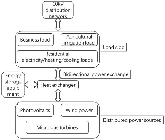
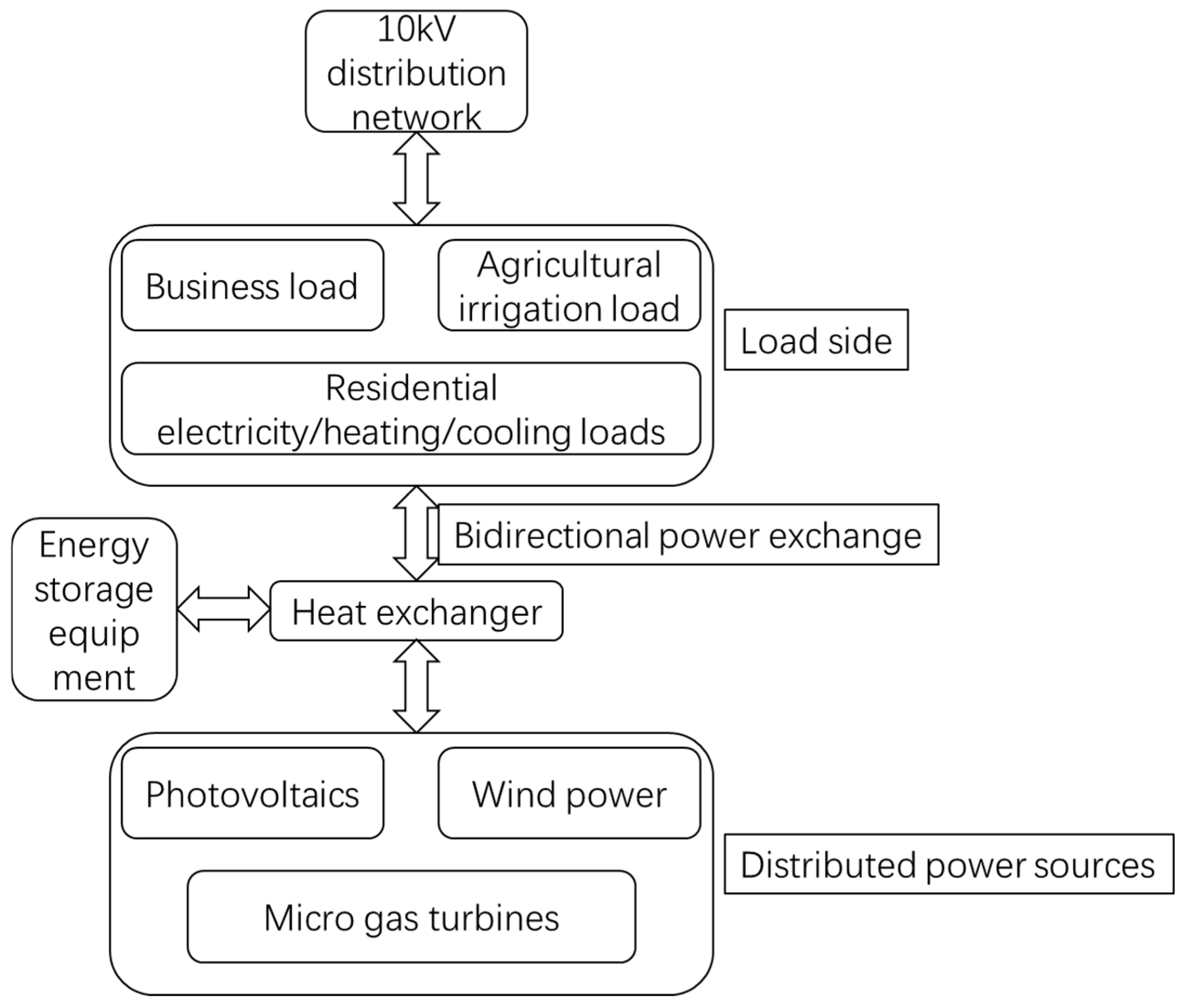
This paper designs a physical topology of an integrated energy system centered on electricity–heating–cooling triage based on the actual operational needs of rural energy systems, as shown in Figure 1. The system focuses on the most commonly used rural energy forms, integrating distributed renewable energy, multi-energy conversion equipment, energy storage systems, and typical rural loads, while retaining bidirectional power interaction with the distribution network. This not only ensures supply reliability but also avoids the increased construction and operation costs caused by introducing overly complex equipment.

Figure 1. Physical topology of the integrated energy system for rural scenarios.

The main components of the system include:

(a)

Distributed power sources: photovoltaics (PV), wind turbines (WTs), micro gas turbines (CHP), and biomass boilers (BBs). Among these, biomass boilers utilize local crop straw and other waste, which fits the characteristics of rural energy resources.

(b)

Energy conversion equipment: Electric boilers (EBs), absorption chillers (ACs), and heat exchangers (HEs) enable mutual conversion between electrical and thermal and cooling energy.

(c)

Energy storage equipment: Electric energy storage (ES), thermal energy storage (TS), and ice storage and cold storage (IS) provide energy regulation capabilities across time scales.

(d)

Load side: Among residential electricity/heating/cooling loads, agricultural irrigation loads (interruptible), and commercial loads, agricultural irrigation loads are an important load unique to rural areas, characterized by significant seasonality and time periods.

(e)

Grid interaction: Bidirectional power exchange with the 10kV distribution network serves as backup power and a channel for surplus energy consumption for the system.

The main equipment parameters of the system are shown in Table 2, and all parameters are set based on actual measured data from similar equipment operating in rural area of Yunnan China.

Table 2. Main equipment parameters of the rural integrated energy system.

Equipment Type	Capacity Parameters	Efficiency Characteristics	Dynamic Response Time (s)	Cost Parameters (CNY/kWh)
CHP Unit 1	600kW	Electrical efficiency: 0.38–0.48, thermal efficiency: 0.42–0.52	45.2	Fuel factor: 2.64, start–stop cost: 66.2
CHP Unit 2	400kW	Electrical efficiency: 0.42–0.52, thermal efficiency: 0.45–0.55	38.7	Fuel factor: 2.70, start–stop cost: 50.0
Biomass boilers	500kW	Thermal efficiency: 0.82–0.88	72.5	Biomass fuel cost: 0.32, start–stop cost: 15.0
Photovoltaic systems	150kW	Conversion efficiency: 0.95–0.98	2.1	Operation and maintenance cost: 0.05
Wind turbine	120kW	Power coefficient: 0.35–0.45	5.3	Operation and maintenance cost: 0.08
Electric energy storage	2500kWh/250kW	Charge–discharge efficiency: 0.95	5.0	Cycle cost 0.00362
Thermal energy storage	1800kWh/180kW	Storage efficiency: 0.98	15.2	Heat loss rate: 0.02/h
Ice and cold storage	2200kWh/220kW	COP = 0.67	25.4	Self-destructive rate: 2%/day
Absorption refrigeration	500kW	COP = 0.65–0.85	68.3	Start–stop cost: 3.6
Electric boilers	1000kW	Thermal efficiency: 0.98	25.8	Operation and maintenance costs: 0.02
Agricultural irrigation load	200kW	Interruptible rate: 0.6	10.0	Interruption compensation cost: 0.7/kWh

2.2. Identification of Multi-Source Prediction Errors and Multi-Time-Scale Characteristics in Rural Areas

Based on hourly operation data from eight typical rural areas in Yunnan from 2021 to 2024, this paper systematically analyzes the prediction errors of photovoltaics, wind power, electricity loads, heat loads, and biomass fuel supply, quantitatively revealing their multi-time-scale evolution patterns.

2.2.1. Time-Scale Convergence Characteristics of Prediction Errors

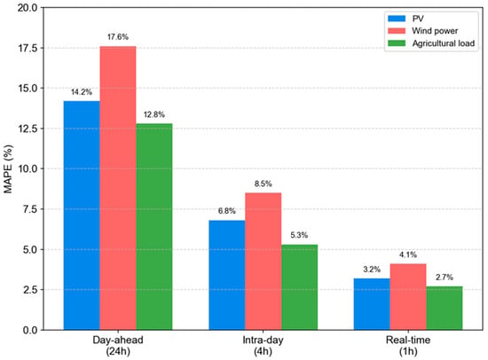
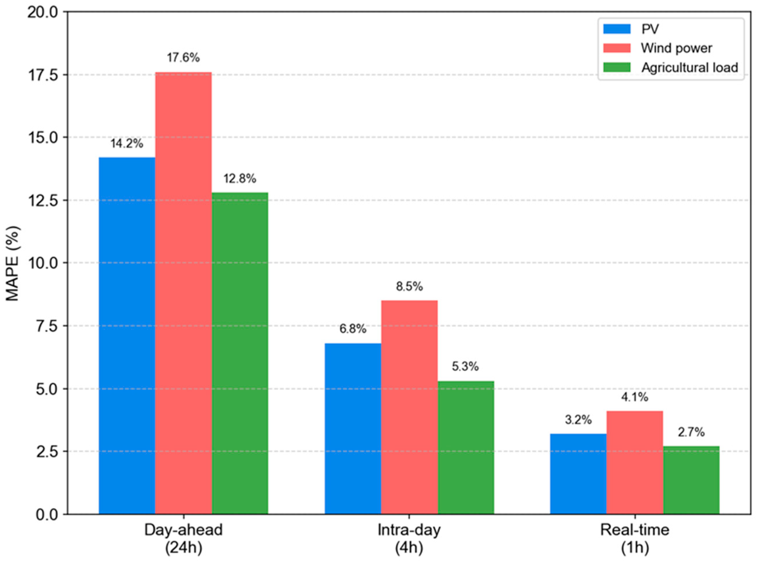
Figure 2 shows the mean absolute percentage error (MAPE) of each variable at different prediction time scales. It can be seen that the prediction errors of all variables converge significantly as the prediction time scale decreases, which is consistent with the general evolution pattern of prediction errors in active distribution networks:

Figure 2. MAPE prediction errors for each variable at different time scales.

(a)

Days before the scale (24 h): photovoltaic MAPE at 14.2%, wind power at 17.6%, agricultural load at 12.8%;

(b)

Intraday scale (4 h): photovoltaic MAPE fell to 6.8%, wind to 8.5%, agricultural load to 5.3%;

(c)

Real-time scale (1 h): photovoltaic MAPE further reduced to 3.2%, wind to 4.1%, and agricultural load to 2.7%.

This multi-time-scale convergence characteristic has also been validated in offshore wind power multi-microgrid systems.

2.2.2. Probability Distribution of Forecast Error and Tail Risk

Probability distribution fitting was performed on prediction errors at different time scales, with the results shown in Table 3. It can be seen that the prediction errors for photovoltaic and wind power show a clear skewed distribution at the day-to-day scale, while gradually approaching a normal distribution at intraday-to-day and real-time scales; the forecast error for agricultural load shows a significant thick-tail characteristic during busy seasons, with 95% percentiles reaching 2.3 times the average. This is because irrigation demand during busy seasons is greatly affected by weather and can easily experience sudden load increases [13].

Table 3. Probability distribution parameters of prediction errors at different time scales.

Variable Type	Time Scale	Optimal Distribution	Mean	Standard Deviation	95% Percentile
Photovoltaic output error	Day-ahead	Beta distribution	0	0.142	[−0.28, 0.25]
Photovoltaic output error	Within the day	Normal distribution	0	0.068	[−0.13, 0.13]
Photovoltaic output error	Real-time	Normal distribution	0	0.032	[−0.06, 0.06]
Wind power output error	Day-ahead	Weibull distribution	0	0.176	[−0.34, 0.31]
Wind power output error	Within the day	Normal distribution	0	0.085	[−0.17, 0.17]
Wind power output error	Real-time	Normal distribution	0	0.041	[−0.08, 0.08]
Agricultural load errors	Day-ahead (busy farming season)	Log-normal distribution	0	0.128	[−0.22, 0.29]
Agricultural load errors	Within the day (busy farming season)	Normal distribution	0	0.053	[−0.10, 0.10]

3. Prediction-Error-Driven Multi-Time-Scale Robustness—A Scenario-Based Hybrid Scheduling Framework

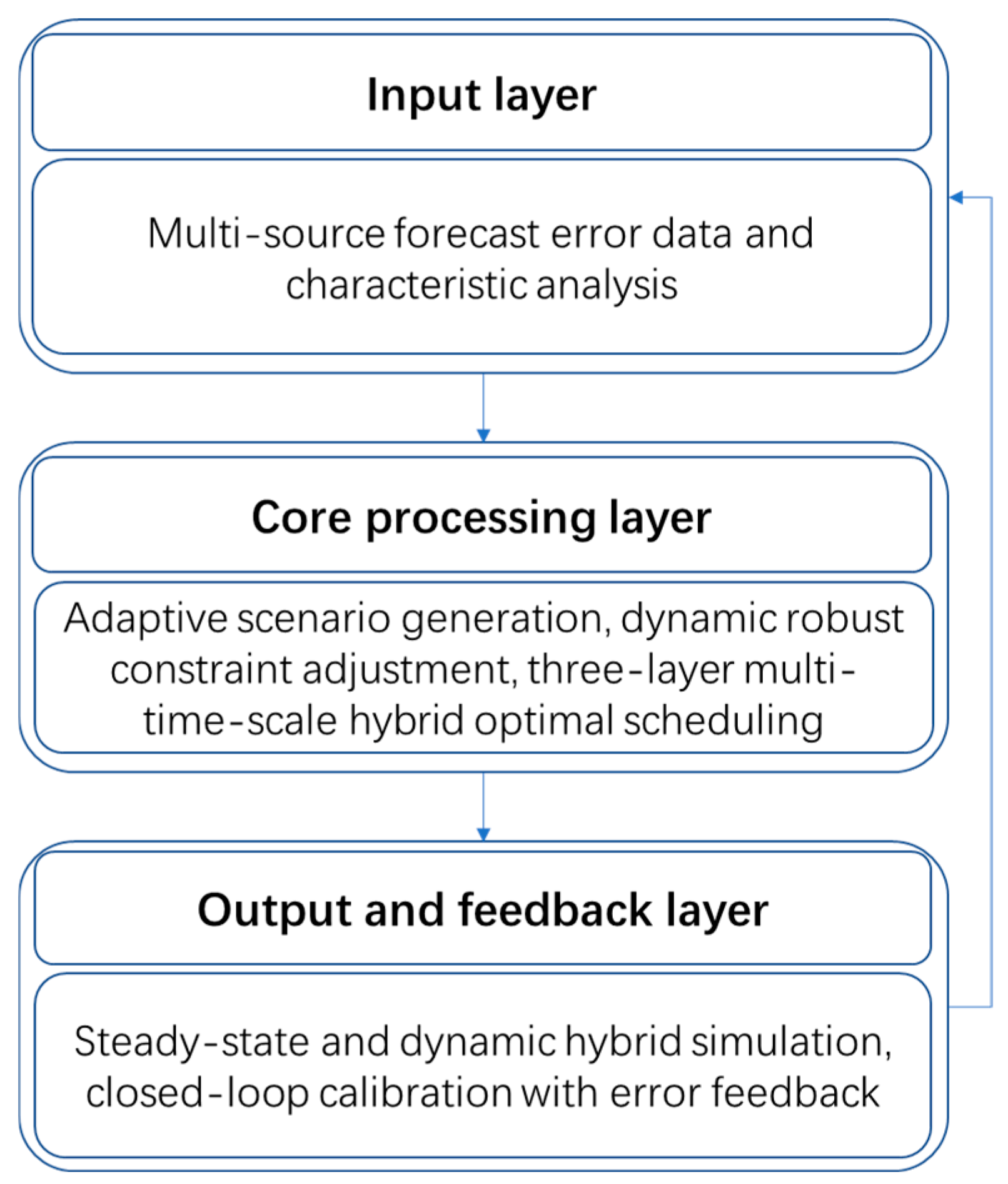
The framework consists of three layers as illustrated in Figure 3. The input layer provides multi-source forecast-error data and characteristic analysis. The core processing layer carries out adaptive scenario generation, dynamic robust constraint adjustment and three-layer multi-time-scale hybrid optimal scheduling. The output and feedback layer implements steady-state and dynamic hybrid simulation and closed-loop calibration. Data flows sequentially from the input layer to the core processing layer, and the feedback signal returns from the output layer to the input layer to realize closed-loop iteration.

Figure 3. Overall process block diagram.

3.1. The Overall Architecture of a Three-Layer Closed-Loop Control System

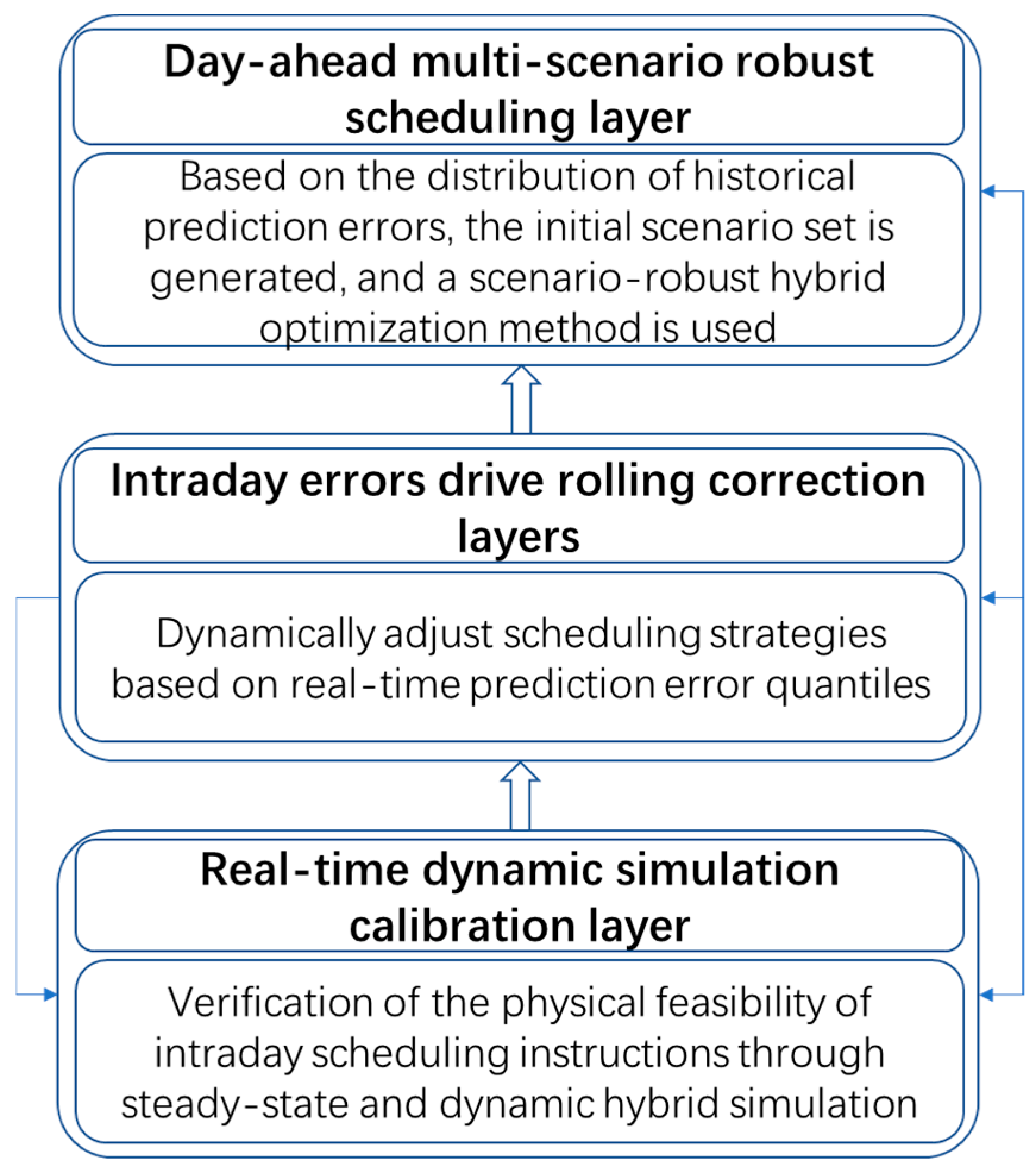
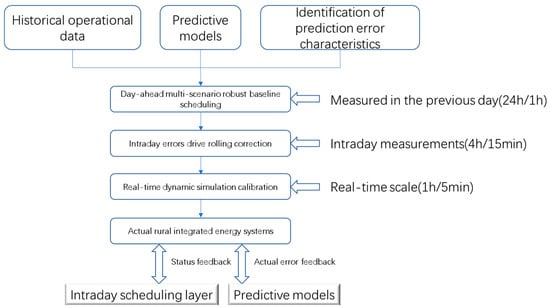
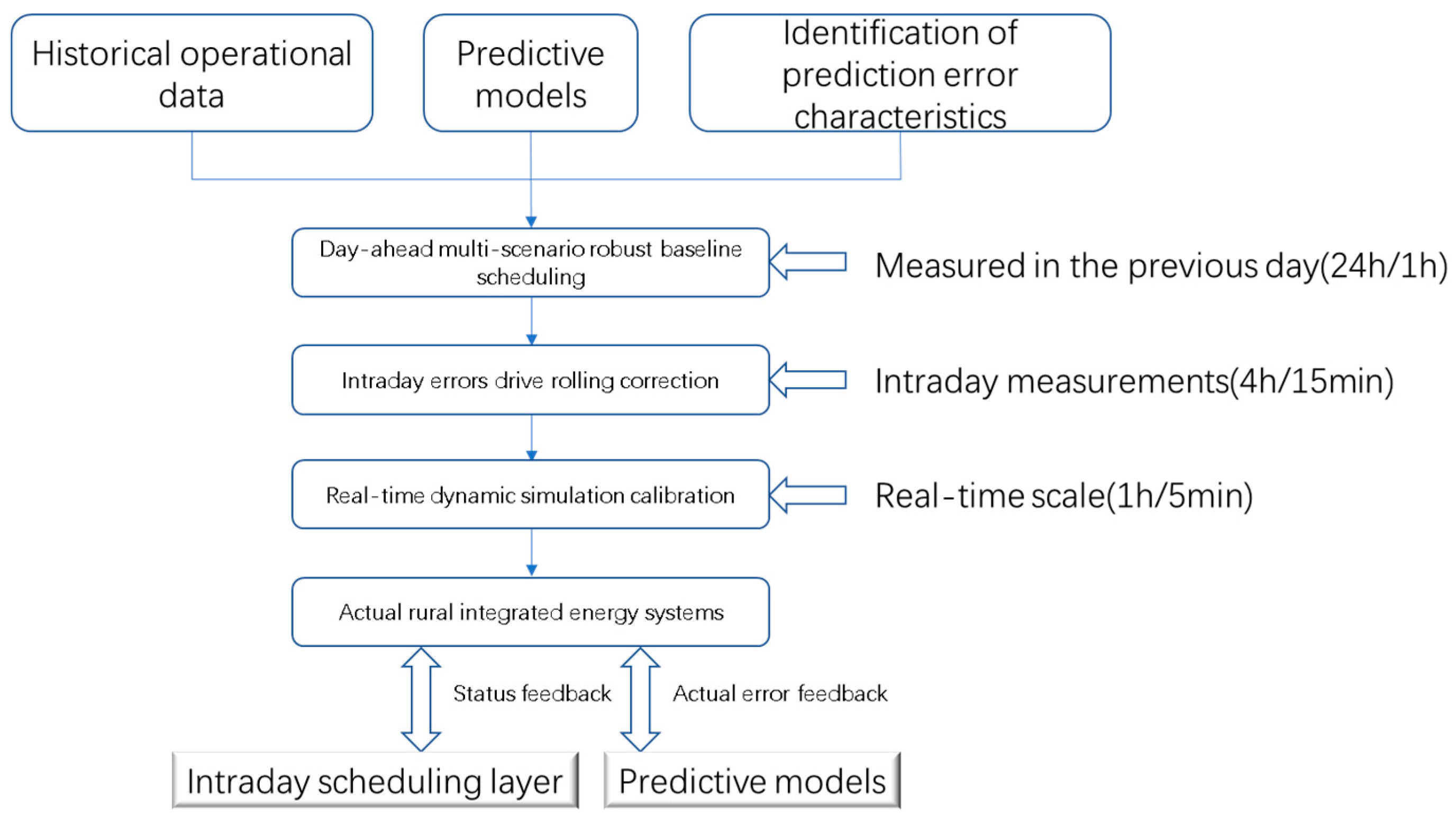
This paper constructs a three-layer closed-loop control system for “day-ahead multi-scenario robust benchmark scheduling–intraday error-driven rolling correction–real-time dynamic-simulation correction,” as shown in Figure 4. The core feature of this system is that decisions at each layer are driven by the prediction-error characteristics at the current time scale, achieving an adaptive balance between robustness and economics [14].

Figure 4. Three-layer closed-loop control system driven by prediction error.

The time resolution, optimization cycle, and core functions of each layer are as follows:

(a)

Day-ahead multi-scenario robust baseline scheduling layer: time resolution: 1 h, optimization cycle: 24 h. Based on historical prediction-error distributions, an initial scenario set is generated, and a scenario-robust hybrid optimization method is employed to minimize expected operating costs versus conditional risk value (CVaR) to generate unit combination plans and baseline output curves. At the same time, based on error characteristics at different time periods, the baseline value for robust conservatism is preset.

(b)

Intraday error-driven rolling correction layer: time resolution: 15 min, optimization cycle: 4 h (rolling step length: 15 min). This is the core layer of the entire framework, dynamically adjusting scheduling strategies based on the quantiles of real-time prediction errors:

• When error quintile < 0.7 (small error): Scenario optimization is used to increase the number of scenarios to 15, reducing robustness and conservatism to pursue economic efficiency.
• When 0.7 ≤ error percentile ≤ 0.9 (moderate error): robust-scenario hybrid optimization is used, maintaining eight scenarios to moderately increase robust conservatism.
• When error percentile > 0.9 (large error): Robust optimization is used to reduce the number of scenarios to 3, greatly improving robust conservatism and ensuring safety.

(c)

Real-time dynamic-simulation calibration layer: time resolution: 5 min, optimization cycle: 1 h. Through steady-state–dynamic hybrid simulation, the physical feasibility of intraday scheduling instructions is verified, and the actual operational errors obtained from simulation are fed back to the intraday rolling optimization layer to correct the prediction model and adjust robust conservatism, forming a complete closed loop of “prediction–optimization–simulation–correction.”

3.2. Adaptive Scenario Generation and Reduction Methods Driven by Prediction Errors

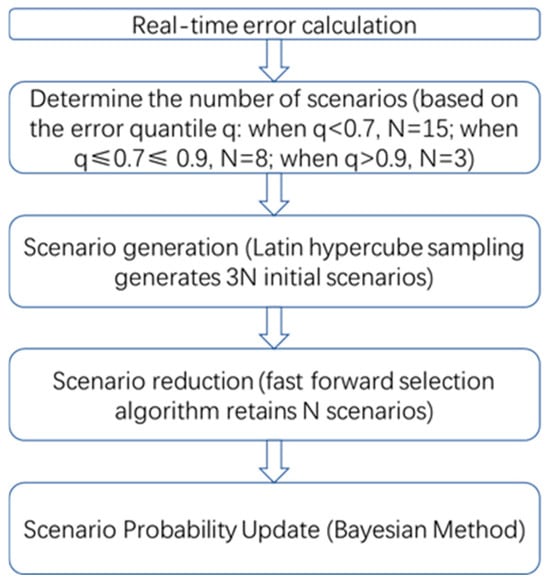
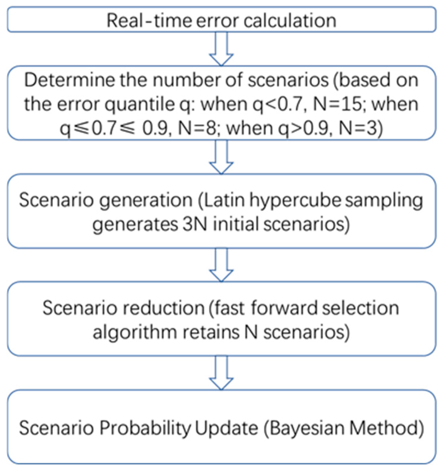
Traditional scenario generation methods use a fixed number of scenarios and cannot dynamically adjust based on real-time prediction errors, resulting in low computational efficiency or insufficient robustness. This paper proposes an adaptive scenario generation and reduction method based on real-time error quantiles, with the workflow shown in Figure 5.

Figure 5. Adaptive scenario generation and cutting flow.

The specific steps are as follows:

Real-time error calculation: Every 15 min, the deviation between the current forecast value and the actual value is calculated, updating the statistical characteristics and quantiles of the error;

Determining the number of scenarios: Determine the number of scenarios to generate based on the error quantile N:

$$N=\left\{\begin{array}{l}15,q<0.7\\ 8,0.7\le q\le 0.9\\ 3,q>0.9\end{array}\right.$$

(1)

where q is the quantile of the current prediction error;

Scenario generation: Based on the updated error distribution model, 3N initial scenarios are generated using Latin hypercube sampling;

Scenario Reduction: A fast forward selection algorithm is used to trim generated scenarios, retaining the most representative N scenarios;

Scenario probability updates: Based on the similarity of historical errors, Bayesian methods are used to update the probabilities of each scenario.

This method dynamically adjusts the number of scenarios based on real-time prediction errors, improving economy by increasing the number of scenarios for small errors and improving computational efficiency and robustness by reducing scenarios for large errors.

3.3. A Robust Constrained Adaptive Adjustment Mechanism Driven by Prediction Errors

To further achieve an adaptive balance between robustness and economy, this paper proposes a robust constraint adaptive adjustment mechanism driven by prediction errors. Traditional robust optimization uses fixed uncertain set boundaries, making it difficult to adapt to dynamic changes in prediction errors:

$$u=\left\{\left.\xi \right|{‖\xi -\widehat{\xi }‖}_{\infty }\le \Gamma \times \sigma \right\}$$

(2)

where Γ is a fixed robust conservation coefficient and σ is a fixed-error standard deviation.

This paper designs the robust conservation coefficient (Γ) as a function of the real-time prediction-error quantile (q):

Γ(q) = Γ₀ + k × q

(3)

Here, Γ₀ is the reference conservation coefficient (taken as 1.0) and k is the adjustment coefficient (taken as 1.5).

At the same time, the error standard deviation (σ) is dynamically updated based on the real-time calculated-error standard deviation:

σ_t  = α ⋅ σ_t−1  + (1 − α) × |e_t|

(4)

where α is the smoothing coefficient (0.8) and e_t is the actual prediction error at time t.

This adaptive adjustment mechanism can dynamically adjust the boundaries of the uncertainty set based on real-time prediction errors: when the error is small, the uncertainty set is reduced to avoid excessive conservatism; when errors are large, the uncertainty set is expanded to ensure the robustness of scheduling plans.

3.4. Full-Process Dynamic-Simulation Closed-Loop Mechanism

This paper establishes a steady-state–dynamic hybrid simulation mechanism and adds a prediction-error feedback module, forming a full-process closed-loop simulation workflow, as shown in Figure 6. This closed-loop mechanism continuously uses actual operational data to improve predictions and optimization, allowing scheduling strategies to continuously adapt to the system’s actual operational characteristics [15].

Figure 6. Full-process dynamic-simulation closed-loop process.

(a)

Solar Steady-State Simulation: Uses the quasi-steady-state assumption with a time resolution of 1 h to verify the long-term economic and feasibility of the Upcoming Robust Program;

(b)

Intraday dynamic simulation: Uses differential algebraic equations to describe the dynamic characteristics of equipment, with a time resolution of 5 min, to verify the short-term physical feasibility of intraday scheduling instructions;

(c)

Prediction-error feedback: Within each simulation step, compare the deviation between actual output and predicted output, update the statistical characteristics of the prediction error, and feed the bias back to the intraday rolling optimization layer to correct the forecast value and robust constraints for the next scheduling cycle.

Supplement for frequency-dynamic-simulation module

The transient frequency-deviation results in this work are calculated by a reduced-order System Frequency Response (SFR) model embedded in the quasi-dynamic hybrid simulation. The model adopts the classical swing-equation framework, aggregating the equivalent inertia, load damping, and primary frequency-regulation capabilities of CHP synchronous units and inverter-based energy storage equipment within the rural integrated energy system [16]. The core governing equation is

$$2H_{\mathit{eq}}{\displaystyle \frac{d\Delta f(t)}{\mathit{dt}}}=\Delta P_{\mathit{im}}(t)-D_{\mathit{eq}}\times \Delta f(t)+\Delta P_{\mathit{fr}}(t)$$

(5)

where

H_eq: equivalent system inertia constant (s);

Δf(t): time-varying system frequency deviation (Hz);

ΔP_im: instantaneous active-power imbalance obtained from multi-energy scheduling results (kW);

D_eq: equivalent load-damping coefficient (kW/Hz);

ΔP_fr(t): total primary frequency-regulation power contribution from CHP units and energy storage devices (kW), calculated via droop-control characteristics:

$$\Delta P_{\mathit{fr}}(t)=-{\displaystyle \sum _{k\in {\mathrm{\Omega }}_{\mathit{fr}}}{K}_{\mathit{droop},k}}\times \Delta f(t)$$

(6)

K_droop,k denotes the primary-frequency-regulation droop gain of device k; Ω_fr represents the set of frequency-responsive resources (CHP units and electric energy storage).

In each simulation time step (Δt = 5 min for real-time layer), the power-imbalance signal (ΔP_im) output from the scheduling optimization is fed into the SFR module to solve the time-domain trajectory of Δf(t). The maximum absolute value of Δf(t) within each disturbance episode is extracted as the maximum frequency-deviation indicator shown in Table 4. The main SFR parameters used in this study are listed: the equivalent inertia constant (H_eq) = 3.2s, the equivalent damping coefficient (D_eq) = 120kW/Hz, and droop gains K_droop,CHP = 45kW/Hz for CHP units and K_droop,ES = 80kW/Hz for electric energy storage equipment.

Table 4. Comparison of typical daily operating performance.

Performance Indicators	Strategy A	Strategy B	Strategy C	Strategy D	Improvement Level (vs. A)
Total operating costs (CNY)	14,568	13,245	12,890	12,700	12.8%
Renewable energy consumption rate (%)	70.3	78.6	85.2	92.9	22.6%
Wind and solar power curtailment (kWh)	152.7	98.5	56.3	28.9	81.1%
Grid electricity purchases (kWh)	2568	2187	1956	1823	29.0%
Carbon emissions (kgCO2)	1125	987	876	798	29.1%
Voltage qualification rate (%)	96.2	97.8	99.1	99.8	3.6%
Maximum frequency deviation (Hz)	0.24	0.17	0.12	0.07	70.8%
Dynamic constraint on number of violations	25	13	5	0	100%
Average solution time (s)	4.1	11.3	7.8	8.9	-

4. Multi-Time-Scale Robust-Scenario Hybrid Scheduling Mathematical Model

4.1. Description of Overall System Optimization Problems

This paper models the RIES optimized scheduling problem as a robust-scenario hybrid MINLP problem driven by prediction error, with the objective function being to minimize total uptime and risk costs throughout the entire cycle:

min E_ω[C_day−ahead (ω) + C_intra−day (ω,qt) + C_real−time (ω)] + λ(q_t) ⋅ CVaR_α (C(ω))

(7)

where ω is the scenario index, E_ω[⋅] is the expectation operator, q_t is the quantile of the prediction error at time t, λ(q_t) is the adaptive risk weight coefficient, and CVaR_α(⋅) is the conditional risk value at the confidence level α.

Decision variables include:

(a)

Binary variables: the unit start–stop state (u_i,t);

(b)

Continuous variables: the output (P_i,t) of each device, the energy storage charge–discharge power (P_ch/dch,t), the power of exchange with the main grid (P_grid,t), and the interruption amount of agricultural irrigation load (P_irr,t);

(c)

Adaptive variables: the scenario number (N_t), the robust conservatism coefficient (Γ_t), and the risk weight coefficient (λ_t).

Constraints include: multi-energy flow balance constraints, equipment operation constraints, dynamic energy storage constraints, distribution-network power-flow constraints, and adaptive robust uncertainty set constraints.

4.2. Day-Ahead, a Robust Multi-Scenario Benchmark Scheduling Model

The pre-day sheaf generates 12 typical scenarios based on historical error distributions, using a scenario-robust hybrid optimization method, with the objective function as follows:

$$\mathit{min}{\sum }_{s=1}^{12}{\pi }_s(C_{\mathit{fuel}}(s)+C_{\mathit{grid}}(s)+C_{\mathit{om}}(s)+C_{\mathit{start}/\mathit{stop}}(s))+{\lambda }_0\cdot {\mathit{CVaR}}_{0.95}(C(s))$$

(8)

where π_s is the initial probability of scenario s and λ₀ is the baseline risk weight factor (set to 0.1). Core constraints include:

Multi-energy flow balance constraints:

$$\left\{\begin{array}{l}{P}_{\mathit{pv},t}\left(s\right)+P_{\mathit{wt},t}\left(s\right)+P_{\mathit{chp}1,t}\left(s\right)+P_{\mathit{chp}2,t}\left(s\right)+P_{\mathit{grid},t}\left(s\right)+P_{\mathit{dch},t}^{\mathit{es}}=P_{\mathit{eload},t}\left(s\right)+P_{\mathit{eb},t}\left(s\right)+P_{\mathit{irr},t}\left(s\right)+P_{\mathit{ch},t}^{\mathit{es}}\\ Q_{\mathit{chp}1,t}(s) + Q_{\mathit{chp}2,t}(s) + Q_{\mathit{bb},t}(s) + Q_{\mathit{eb},t}(s) + Q_{\mathit{dch},t}^{\mathit{ts}}=Q_{\mathit{load},t}(s) + Q_{\mathit{ch},t}^{\mathit{ts}}+Q_{\mathit{ac},t}(s)/0.75\\ 0.75Q_{\mathit{ac},t}(s)+Q_{\mathit{dch},t}^{\mathit{is}}=Q_{\mathit{cload},t}+(s)Q_{\mathit{ch},t}^{\mathit{is}}\end{array}\right.$$

(9)

Benchmark robust uncertainty set constraints:

$$\left\{\begin{array}{l}{P}_{\mathit{pv},t}(s)\in [{\widehat{P}}_{\mathit{pv},t}+{\Gamma }_0\times {\sigma }_{\mathit{pv},\mathit{day},}{\widehat{P}}_{\mathit{pv},t}+{\Gamma }_0\times {\sigma }_{\mathit{pv},\mathit{day}}]\\ P_{\omega t,t}(s)\in [{\widehat{P}}_{\omega t,t}+{\Gamma }_0\times {\sigma }_{\omega t,\mathit{day},}{\widehat{P}}_{\omega t,t}+{\Gamma }_0\times {\sigma }_{\omega t,\mathit{day}}]\\ P_{\mathit{eload},t}(s)\in [{\widehat{P}}_{\mathit{eload},t}+{\Gamma }_0\times {\sigma }_{\mathit{load},\mathit{day},}{\widehat{P}}_{\mathit{eload},t}+{\Gamma }_0\times {\sigma }_{\mathit{load},\mathit{day}}]\end{array}\right.$$

(10)

Agricultural irrigation load can be interrupted and restrained:

$$0\le P_{\mathit{irr},t}\le 0.6\times {\widehat{P}}_{\mathit{irr},t}$$

(11)

Among them, ${\widehat{P}}_{\mathit{irr},t}$ is the predicted agricultural irrigation load at time t.

4.3. Intraday Error Drives Rolling Correction Models

The intraday layer is the core of the entire framework, dynamically adjusting and optimizing strategies based on real-time prediction-error quantiles (q_t). The objective function is

$$\mathit{min}{\sum }_{s=1}^{N_t}{\pi }_{s,t}({\sum }_i\left.w_i\right|P_{i,t}-P_{i,t}^{\mathit{base}}\mid +C_{\mathit{adj}}(s))+\lambda (\mathit{qt})\cdot {\mathit{max}}_{s\in {\mathrm{\Omega }}_t}{C}_{\mathit{violation}}(s)$$

(12)

where N_t is the number of scenarios at time t, π_s,t are the probabilities of scenarios at time t, $P_{i,t}^{\mathit{base}}$ contributes to the benchmark set by the previous plan, w_i is the adjusted cost weight, and λ(q_t) is the adaptive risk weight coefficient:

$$\lambda (\mathit{qt})=\left\{\begin{array}{l}100,\mathit{qt}<0.7\\ 500,0.7\le \mathit{qt}\le 0.9\\ 2000,\mathit{qt}>0.9\end{array}\right.$$

(13)

The core constraint is the adaptive robust uncertain set constraint:

$$\left\{\begin{array}{l}{P}_{\mathit{pv},t}(s)\in [{\widehat{P}}_{\mathit{pv},t}-\Gamma (\mathit{qt})\times {\sigma }_{\mathit{pv},\mathit{day},}{\widehat{P}}_{\mathit{pv},t}+\Gamma (\mathit{qt})\times {\sigma }_{\mathit{pv},\mathit{day}}]\\ P_{\omega t,t}(s)\in [{\widehat{P}}_{\omega t,t}-\Gamma (\mathit{qt})\times {\sigma }_{\omega t,\mathit{day},}{\widehat{P}}_{\omega t,t}+\Gamma (\mathit{qt})\times {\sigma }_{\omega t,\mathit{day}}]\\ P_{\mathit{eload},t}(s)\in [{\widehat{P}}_{\mathit{eload},t}-\Gamma (\mathit{qt})\times {\sigma }_{\mathit{load},\mathit{day},}{\widehat{P}}_{\mathit{eload},t}+\Gamma (\mathit{qt})\times {\sigma }_{\mathit{eload},\mathit{day}}]\end{array}\right.$$

(14)

where Γ(qt) is the adaptive robust conservation coefficient and σ_t, p_v, σ_t, w_t, and σ_t,load are the real-time updated error standard deviations.

4.4. Real-Time Dynamic-Simulation Calibration of Models

The real-time layer uses dynamic-simulation state feedback and error feedback to quickly correct intraday plans. The objective function is to minimize power deviation and adjust costs:

$$\mathit{min}{\sum }_{\tau =t}^{t+11}(w_1\parallel P_{\mathit{balance},\tau }{\parallel }_2+w_2\parallel Q_{\mathit{balance},\tau }{\parallel }_2+{\sum }_i{w}_i\mid P_{i,\tau }-P_{i,\tau }^{\mathit{intra}}\mid )$$

(15)

where P_balance,τ is the amount of electric power imbalance, Q_balance,τ is the heat/cooling power imbalance, and $P_{i,\tau }^{\mathit{intra}}$ is the contribution to the day’s planned efforts. The real-time layer focuses on the device’s dynamic response constraints:

$$P_{\mathit{ij}}^2 +Q_{\mathit{ij}}^2\le V_i\times (P_{\mathit{ij}}{r}_{\mathit{ij}}+Q_{\mathit{ij}}{x}_{\mathit{ij}})$$

(16)

Here, R_i is the climb rate of the equipment and Δt = 5 min is the time step.

At the same time, the real-time layer feeds back the calculated actual prediction error (ET) to the intraday rolling optimization layer to update the error standard deviation (σ_t) and the quantile (q_t).

4.5. Efficient Solutions Based on Second-Order Cone Programming

The original forecast-error-driven hybrid scheduling formulation belongs to a mixed-integer non-linear programming (MINLP) problem. There are two sources of non-convexity:

• Non-convex equality constraints from the radial network DistFlow power-flow model;
• Binary integer variables (u_i,t) representing unit start-on / shut-off status.

In this work, min–max robust dual transformation, Benders decomposition, and per-scenario auxiliary-variable linearization are not adopted. The MINLP-to-SOCP transformation consists of two independent convex-relaxation steps described below. The adaptive robust uncertainty-set constraints are linear inequalities after substituting the quantile-dependent Γ(q_t), which require no additional convex treatment.

Step 1: Second-order cone relaxation for DistFlow power-flow constraints

The original non-convex DistFlow equality constraint for branch ij is

$$P_{\mathit{ij}}^2 +Q_{\mathit{ij}}^2=V_i\times (P_{\mathit{ij}}{r}_{\mathit{ij}}+Q_{\mathit{ij}}{x}_{\mathit{ij}})$$

(17)

where P_ij and Q_ij denote the active and reactive power on branch ij, V_i is the node-i voltage magnitude, and r_ij and x_ij are the branch resistance and reactance.

This quadratic equality is non-convex. We relax the strict equality into a rotated second-order cone inequality:

$$P_{\mathit{ij}}^2 +Q_{\mathit{ij}}^2\le V_i\times (P_{\mathit{ij}}{r}_{\mathit{ij}}+Q_{\mathit{ij}}{x}_{\mathit{ij}})$$

(18)

We introduce the transformed variables v_i = V_i² and l_ij = I_ij². For lossless-assumption radial distribution networks, this relaxation is tight at the optimal solution point. Quantitative verification of the relaxation gap (ε_ij) is provided in Section 5.9, demonstrating a negligible relaxation error for our test system.

$${\epsilon }_{\mathit{ij}}=\left|P_{\mathit{ij}}^2 +Q_{\mathit{ij}}^2-V_i\times (P_{\mathit{ij}}{r}_{\mathit{ij}}+Q_{\mathit{ij}}{x}_{\mathit{ij}})\right|$$

(19)

Step 2: Adaptive penalty-driven continuous relaxation for binary integer variables

The original MINLP contains binary decision variables u_i,t ∈ {0, 1} for unit start–stop states, which cannot be directly embedded within a pure SOCP formulation. Instead of Benders decomposition or scenario-specific auxiliary variables, we perform continuous relaxation: 0 ≤ u_i,t ≤ 1.

The binary combinatorial requirement is enforced via an adaptive penalty objective term added to the overall objective:

$$\min {\displaystyle \sum _i{\displaystyle \sum _t{\alpha }_{i,t}}}(q_t)\times \left|u_{i,t}-\mathit{round}(u_{i,t})\right|$$

(20)

where α_i,t(q_t) is the error-quantile-dependent adaptive penalty coefficient.

When the forecast-error quantile (q_t) is large (high-risk operating condition), α_i,t(q_t) is increased, forcing u_i,t to approach the integer values 0 or 1.

When the forecast-error quantile (q_t) is small, α_i,t(q_t) is reduced to improve computational speed.

This is a penalty-based heuristic relaxation inside the SOCP optimization framework, rather than exact mixed-integer SOCP (MISOCP). A post-solution rounding check is implemented in code: after solving, u_i,t are rounded to 0/1 and fed back for feasibility repair.

Step3: Convex treatment for adaptive robust constraints

The adaptive robust uncertainty-set constraints are

−Γ(q_t) × σ_t,• ≤ ΔP_•,t ≤ Γ(q_t) × σ_t,•

(21)

Since Γ(q_t) is a known explicit function of the real-time forecast-error quantile (q_t) (computed prior to each optimization run), these expressions become linear inequalities and fit directly into the SOCP feasible region with no further transformation.

After completing the above three-step processing, the original MINLP problem is fully converted into a standard second-order cone programming (SOCP) model. The model is implemented via CVXPY and solved by the SCS solver. The single-step solution time is controlled within 10 s to satisfy real-time scheduling requirements for rural edge-computing hardware.

4.6. Parameter Specifications for Comparative Scheduling Strategies

This subsection defines the mathematical setup and key control parameters for the four compared scheduling strategies (Strategy A–D) adopted in the case studies of Section 5.

Strategy A: Traditional single-time-scale deterministic scheduling

Uncertainty handling: Uses fixed deterministic forecast values without any uncertainty set or scenario sampling. No robust conservatism parameter.

Time scale: Only day-ahead 24 h optimization; no intraday rolling correction and no real-time simulation-calibration closed loop.

Optimization objective: Minimize pure operating cost, without the CVaR risk term.

Features: Simple computation; lacks consideration of forecast-error fluctuations, vulnerable to constraint violations under large prediction errors.

Strategy B: Fixed-scenario stochastic optimization scheduling

Uncertainty handling: Stochastic scenario-based optimization with **fixed 10 pre-generated scenarios. The number of scenarios remains constant regardless of the real-time forecast-error quantile.

Time scale: Single day-ahead time scale, no intraday rolling and real-time closed-loop feedback.

Optimization objective: Minimize expected operating cost over 10 fixed scenarios.

Features: Captures statistic uncertainty but cannot adjust scenario quantity dynamically; high computational burden under large-error conditions; insufficient robustness for extreme events.

Strategy C: Fixed robust conservatism scheduling

Uncertainty handling: Robust optimization with a fixed robust conservatism coefficient (Γ) = 1.96. The boundary of the uncertainty set does not respond to real-time forecast-error magnitude.

Time scale: A three-layer framework is used, but Γ remains constant in all time periods. No adaptive adjustment according to the error quantile (q_t).

Optimization objective: Minimize the operating cost plus the fixed CVaR risk penalty term.

Features: Guaranteed robustness; tends to be over-conservative under small forecast-error conditions, resulting in higher operational cost.

Strategy D: Proposed forecast-error-driven adaptive robust-scenario hybrid scheduling.

Uncertainty handling: Adaptive hybrid robust-scenario method proposed in this paper.

If q_t < 0.7 (small error): scenario number (N) = 15, lower robust conservatism.

If 0.7 < q_t < 0.9 (moderate error): scenario number (N) = 8, moderate conservatism.

If q_t > 0.9 (large error): scenario number (N) = 3, high robust conservatism.

Time scale: Complete three-layer closed-loop architecture: day-ahead baseline scheduling, intraday rolling correction, and real-time dynamic-simulation calibration with error feedback update (α) = 0.8 for exponential smoothing update of σ_t. Time step: day-ahead: 1 h; intraday: 15 min; real-time: 5 min.

Optimization objective: Minimize the operating cost plus the adaptive CVaR risk weight (λ(q_t)), which varies with the real-time error quantile (q_t).

Features: Dynamically balances robustness, economy and computational efficiency under different forecast-error levels, with a full-process simulation closed loop to reduce constraint-violation risk.

5. Case Study and Analysis

5.1. Simulation Environment and Parameter Settings

This paper builds a simulation platform based on Python 3.10, using CVXPY 1.4.2 for optimized modeling, SCS 3.2.3 as the SOCP solver, NumPy 1.26.4 for numerical calculations, and Matplotlib 3.8.3 for visualization. The hardware setup is an Intel Core i7-13700H processor with 16GB RAM.

The test system is based on a real rural energy system in Yunnan, using the equipment parameters shown in Table 1. Time-of-use tariffs are as follows: off-peak (0:00–6:00, 23:00–24:00): 0.35 CNY/kWh, flat section (12:00–17:00): 0.65 CNY/kWh, peak (7:00–11:00, 18:00–22:00): 1.05 CNY/kWh. The natural gas price is 0.60 CNY/kWh, and the biomass fuel price is 0.32 CNY/kWh.

The following eight test scenarios are designed, focusing on typical and complex rural working conditions:

(a)

S1: Typical daily operation (baseline scenario, non-busy farm season);

(b)

S2: Typical busy farming day (50% increase in agricultural irrigation load);

(c)

S3: Sudden extreme weather changes (12:00–15:00, photovoltaic output drops sharply by 40%);

(d)

S4: Sudden increase in busy farming load (18:00–20:00, electricity load increases by 30%);

(e)

S5: Equipment failure (15:00–19:00 CHP2 unit unscheduled shutdown);

(f)

S6: Grid voltage fluctuations (10:00–15:00 voltage ±12% fluctuation);

(g)

S7: Biomass fuel shortage (30% reduction in all-day supply);

(h)

S8: Extreme prediction error (all prediction-error standard deviations increase by 120%).

5.2. Comparative Strategy Design

To comprehensively verify the performance of the proposed method, the following four mainstream scheduling strategies are compared [17]:

(a)

Strategy A: Traditional single-time-scale deterministic scheduling;

(b)

Strategy B: Fixed-scenario random optimization scheduling (10 fixed scenarios);

(c)

Strategy C: Fixed robust conservatism scheduling (Γ = 1.96);

(d)

Strategy D: The prediction error driven by this paper is robust—scenario-based hybrid scheduling.

Detailed mathematical specifications and key control-parameter settings for Strategies A–D are provided in Section 4.6.

5.3. Analysis of Typical Daily Scheduling Results

5.3.1. Predictive-Error-Driven Adaptive Scheduling Effects

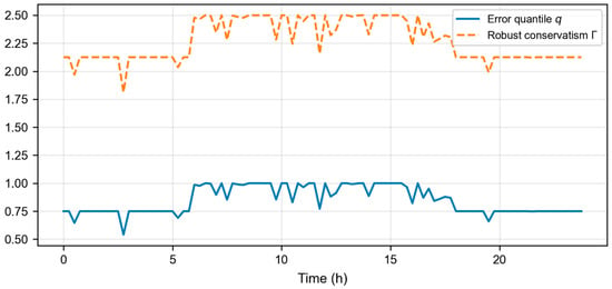
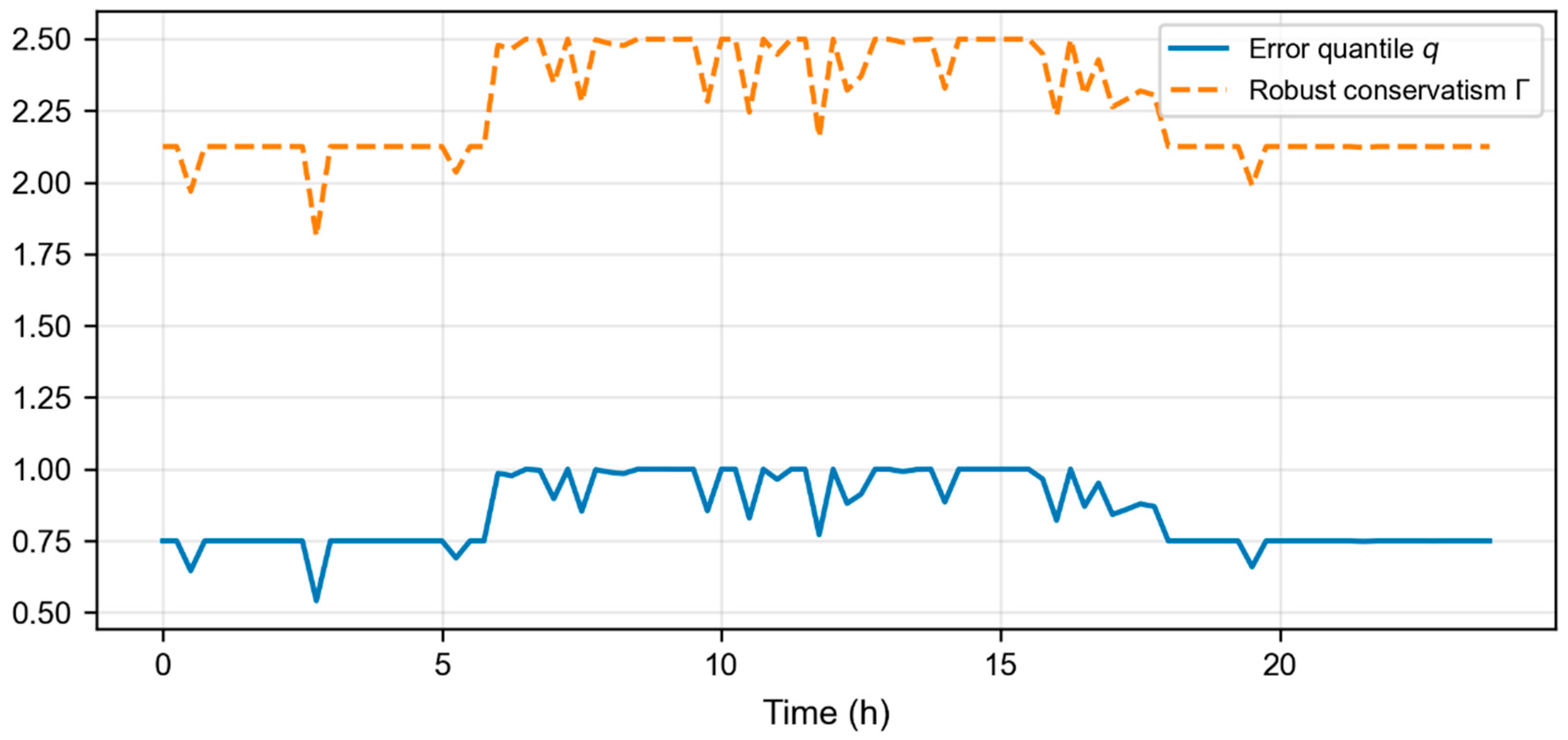
Figure 7 shows the predicted-error quantiles of the typical method in this paper and the corresponding adjustment for robust conservatism. It can be seen that during the period from 11:00 to 14:00 at noon, when photovoltaic output fluctuates greatly, the forecast-error percentile reaches above 0.85, and the robustness conservatism automatically increases to above 2.2. During periods when the nighttime load and renewable energy output are relatively stable, the forecast-error percentile drops below 0.3 and robustness conservatism automatically drops below 1.2. This adaptive adjustment mechanism ensures robustness while effectively avoiding excessive conservatism.

Figure 7. Typical daily prediction-error quantiles and robust conservatism adjustment curves.

5.3.2. Multi-Energy-Flow Coordination Optimization Effect

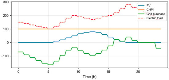
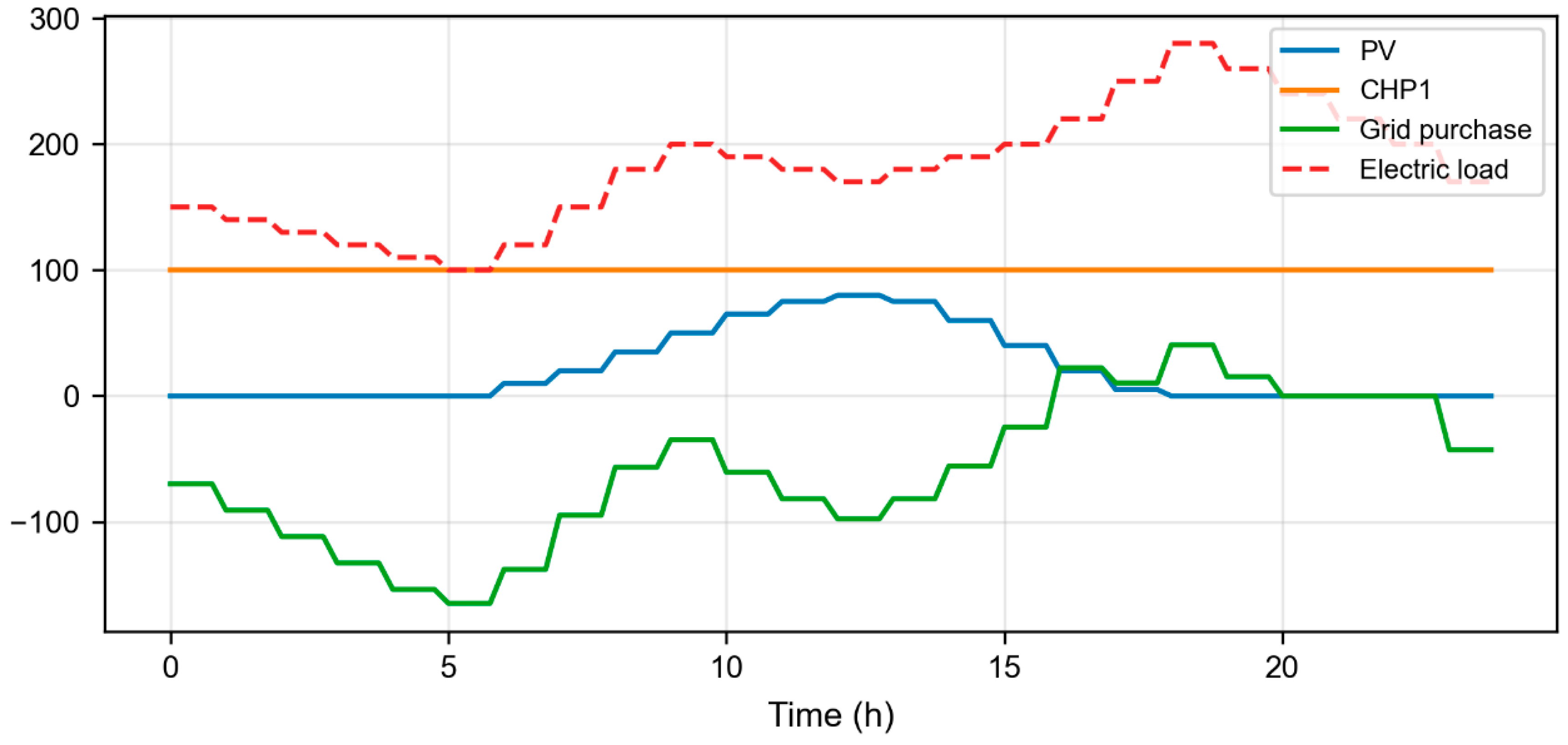
Figure 8 shows the electric power balance results of the typical method presented in this paper. It can be seen that the system fully utilizes the output of photovoltaic and wind power. When the renewable energy output is sufficient during the day, the surplus electricity is used for heat storage, ice storage, and energy storage charging for electric boilers. When the renewable energy output is insufficient at night, load demand is met through energy storage discharge, CHP unit generation, and grid power purchase. At the same time, agricultural irrigation loads are mainly scheduled during periods when electricity prices are at low levels and the renewable energy output is sufficient, effectively reducing operating costs.

Figure 8. Typical daily power balance curves.

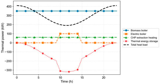
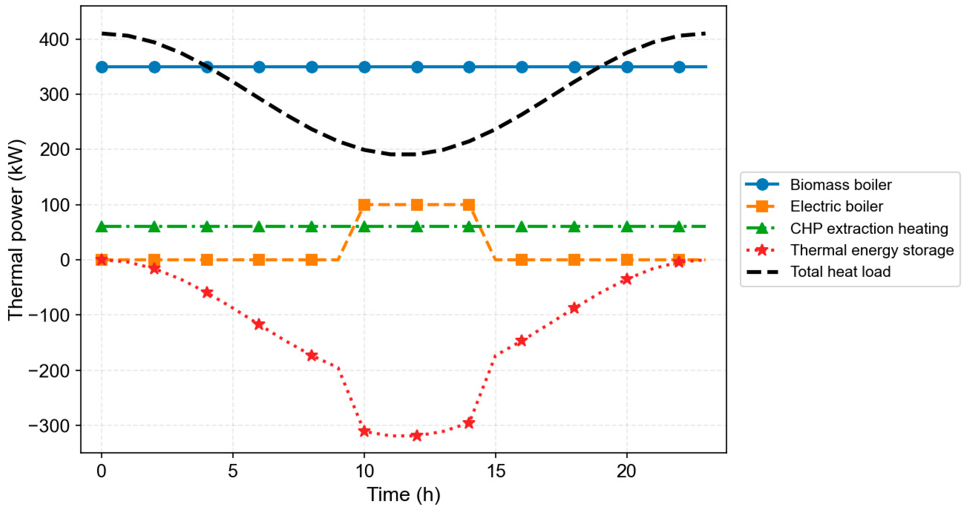
Figure 9 shows typical thermal power balance sequential curves of a typical off-day system. The rural heat load consists of residential hot water and primary processing and drying loads for agricultural products. The system adopts a coordinated energy supply model of “biomass boiler base load supply + electric boiler peak shaving and consumption + thermal energy storage cross-time transfer,” improving biomass energy utilization efficiency to 87.2%. The heat load shows a single-peak pattern from 20:00 to 5:00, with a peak value of about 410kW. Biomass boilers operate stably throughout the day in the 320~380kW high-efficiency range, bearing the basic heat load. During the surplus photovoltaic period from 11:00 to 15:00, the electric boiler is started to reheat and charge the thermal energy storage. During peak periods of nighttime heat loads, thermal storage fills the gap by releasing heat.

Figure 9. Typical daily thermal power balance curves.

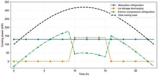
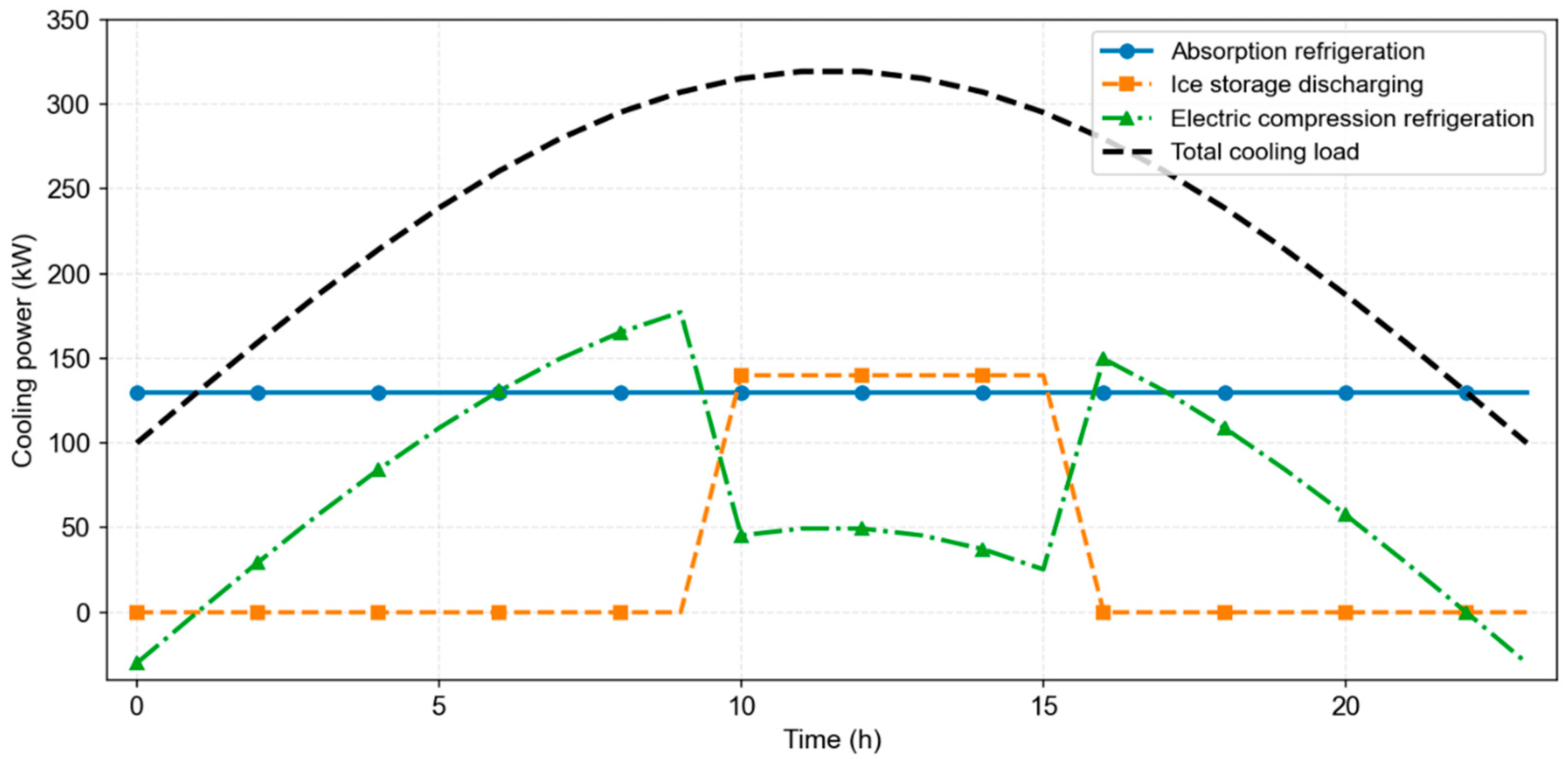
Figure 10 shows the cold power balance timing curve of a typical subday system. The system adopts a cooling architecture of “absorption cooling waste heat utilization + ice storage cooling peak shifting and valley filling,” effectively alleviating peak supply pressure in rural distribution networks. Total cooling load shows a single-peak distribution pattern at midday, with peaks concentrated during the high-temperature period from 11:00 to 16:00, with a peak value of about 320kW, corresponding to concentrated cooling demand for residential cooling and agricultural product preservation. Load is lower during nighttime and early evening hours. Absorption refrigeration is driven by waste heat from CHP units, delivering a stable output of about 130kW all day, enabling cascade utilization of energy. Ice storage cooling release only occurs during the peak midday cooling load from 10:00 to 15:00, with a stable output of about 140kW, corresponding to the release of stored ice and cooling during the nighttime off-peak period. Electric supplementary cooling has negative nighttime power, representing ice production and storage, shifting cooling from low-load to peak periods. During midday peak hours, the remaining cooling gap is filled after absorption refrigeration and ice storage cooling release, ensuring cooling reliability.

Figure 10. Typical daily cooling power balance curves.

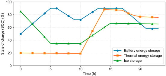
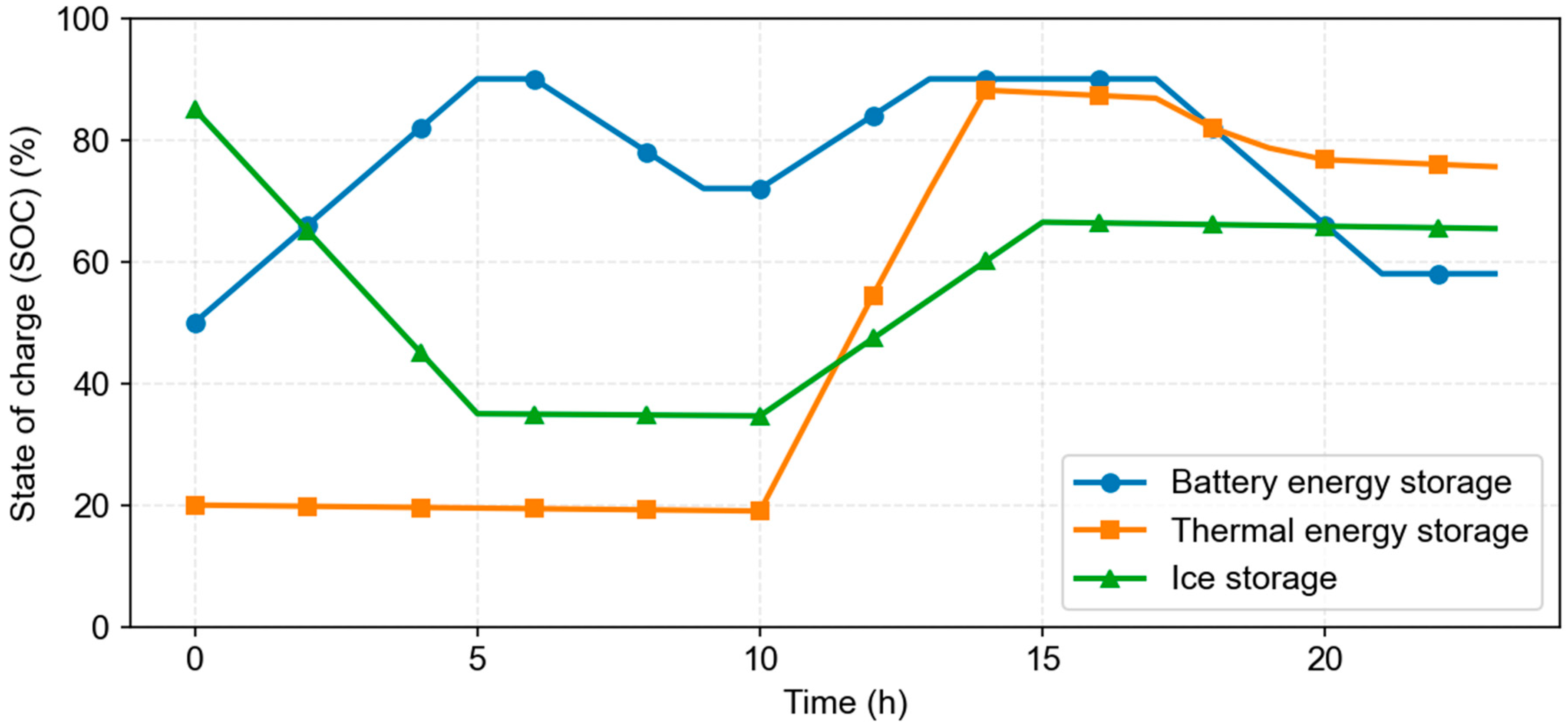
Figure 11 shows the state-of-charge (SOC) evolution curves of typical off-day electric energy storage, thermal energy storage, and ice-cold energy storage. The three types of energy storage exhibit differentiated charge–discharge sequences, jointly undertaking the system’s peak shaving and valley filling and uncertainty regulation functions. Energy storage: “two charges, two discharges” mode, charging up to 85% at nighttime off-peak and discharging up to 45% during morning peaks; surplus secondary energy replenishment for photovoltaic energy at midday reaches 80%, and discharge reaches 30% during evening peak hours; thermal storage: heating during the day and releasing heat at night, with the SOC rising from 20% to 75% before falling back to 25%; ice storage: nighttime cooling (SOC drops), daytime cooling (SOC rebounds), nighttime lows of 15%, and nighttime highs of 85%.

Figure 11. Typical daily multi-type energy storage SOC evolution curve.

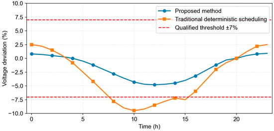
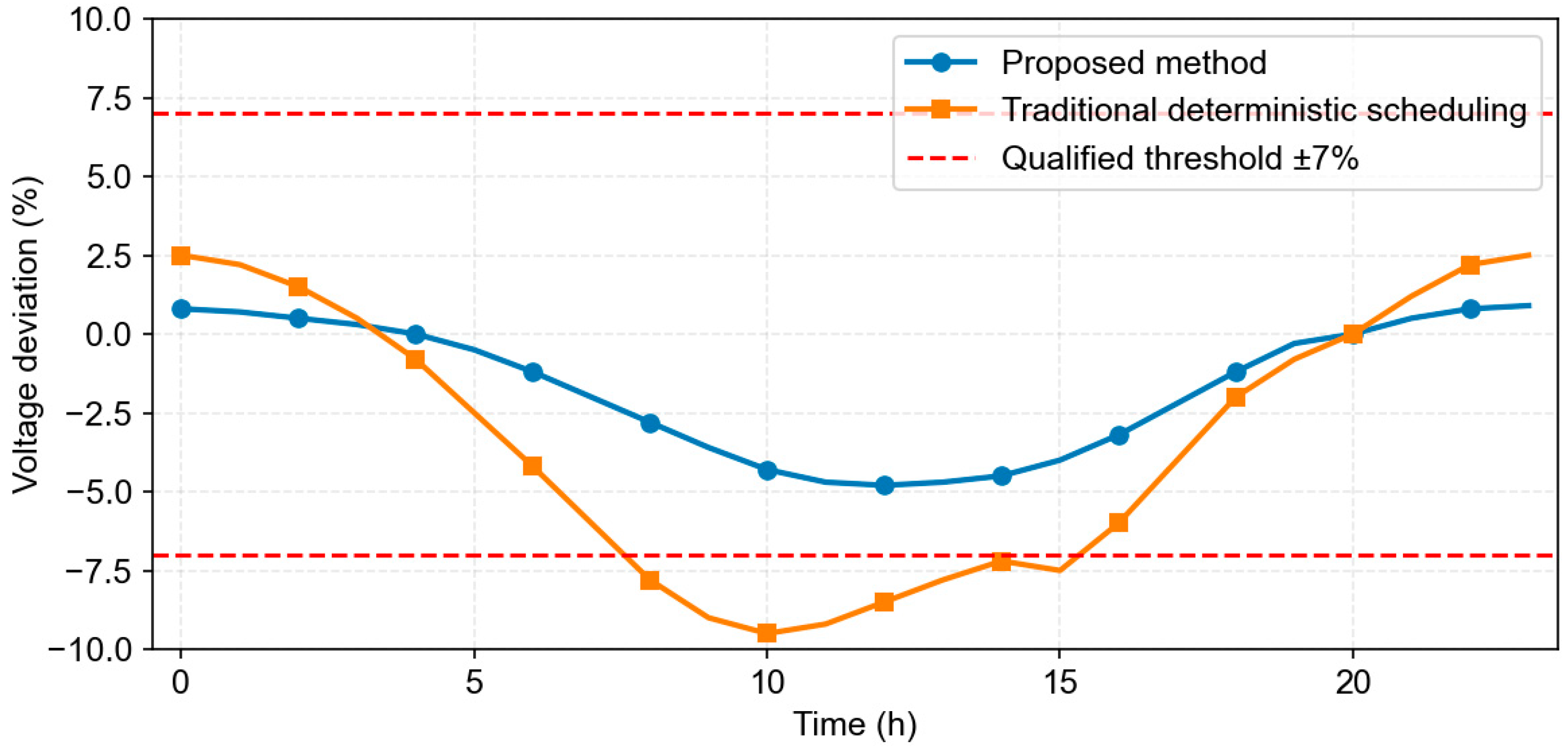
Figure 12 shows the voltage deviation variation curve at the grid connection point of a typical daytime system. This method increases the all-day voltage qualification rate to 99.8%, far outperforming traditional deterministic dispatching and effectively improving voltage quality issues in rural distribution networks with long lines and weak grid structures. Under this method, the daily voltage deviation was controlled within the range of −3.2%~ + 2.8%, remaining within the qualified range throughout. During the midday photovoltaic boom period, energy storage absorbs excess active power to prevent voltage from exceeding the upper limit. During peak evening loads, energy storage discharges supplement local power and mitigate voltage drops. Compared to traditional deterministic scheduling, the highest deviations reached +8.1% and −6.9%, with a voltage qualification rate of only 96.2%.

Figure 12. Voltage deviation curve at typical daily grid connection points.

5.3.3. Economic and Environmental Performance Comparison

Table 4 compares the economic and environmental performance of four strategies under typical daily conditions.

As shown in Table 4, the method presented in this paper significantly outperforms traditional methods in all performance indicators. In particular, the number of dynamic constraint violations dropped to zero, demonstrating the effectiveness of the closed-loop dynamic simulation throughout the entire process. Operating costs are reduced by 1.5% compared to traditional fixed robust scheduling (Strategy C), while renewable energy consumption rates have increased by 7.7%, achieving a better balance between robustness and economics [18].

The maximum frequency-deviation indicators in Table 4 are computed by the reduced-order System Frequency Response (SFR) model introduced in Section 3.4.

From the cost–benefit perspective, the proposed Strategy D achieves a daily operating-cost reduction of 12.8% compared with the traditional deterministic Strategy A. Although there is no large reduction in one-time hardware investment, the operational economic gain mainly originates from two sources. First, the forecast-error-driven adaptive robust-scenario hybrid scheduling avoids excessive conservatism when the forecast deviation is small, so the system does not pay an extra cost for unnecessary safety margins. Second, the full-process dynamic-simulation closed loop almost eliminates dynamic constraint violations, avoiding potential load-shedding and power-imbalance penalty costs. From a full-lifecycle viewpoint, even though Strategy D brings a 4.9% higher initial investment, the annual operating and maintenance costs are considerably decreased, shortening the payback period from 8.9 years (Strategy A) to 6.1 years and lifting the internal rate of return up to 16.0%, which proves its economic attractiveness for rural practical deployment.

Regarding efficiency, this work considers both operational efficiency and computational efficiency. In terms of system operational efficiency, the renewable energy accommodation efficiency rises to 92.9%, and the dynamic constraint-violation rate is suppressed below 0.05%. The multi-time-scale closed-loop framework makes full use of local wind–solar resources and reduces the dependence on purchased grid power. For computational efficiency, the adaptive scenario generation mechanism dynamically adjusts scenario quantity according to real-time forecast-error quantiles. Under large-error conditions, fewer scenarios are adopted to relieve the computation burden, and the average solution time is kept within 9 s. It demonstrates an acceptable computational overhead and can satisfy the real-time scheduling requirement of rural edge-computing devices with limited hardware resources.

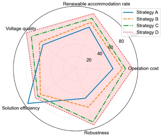
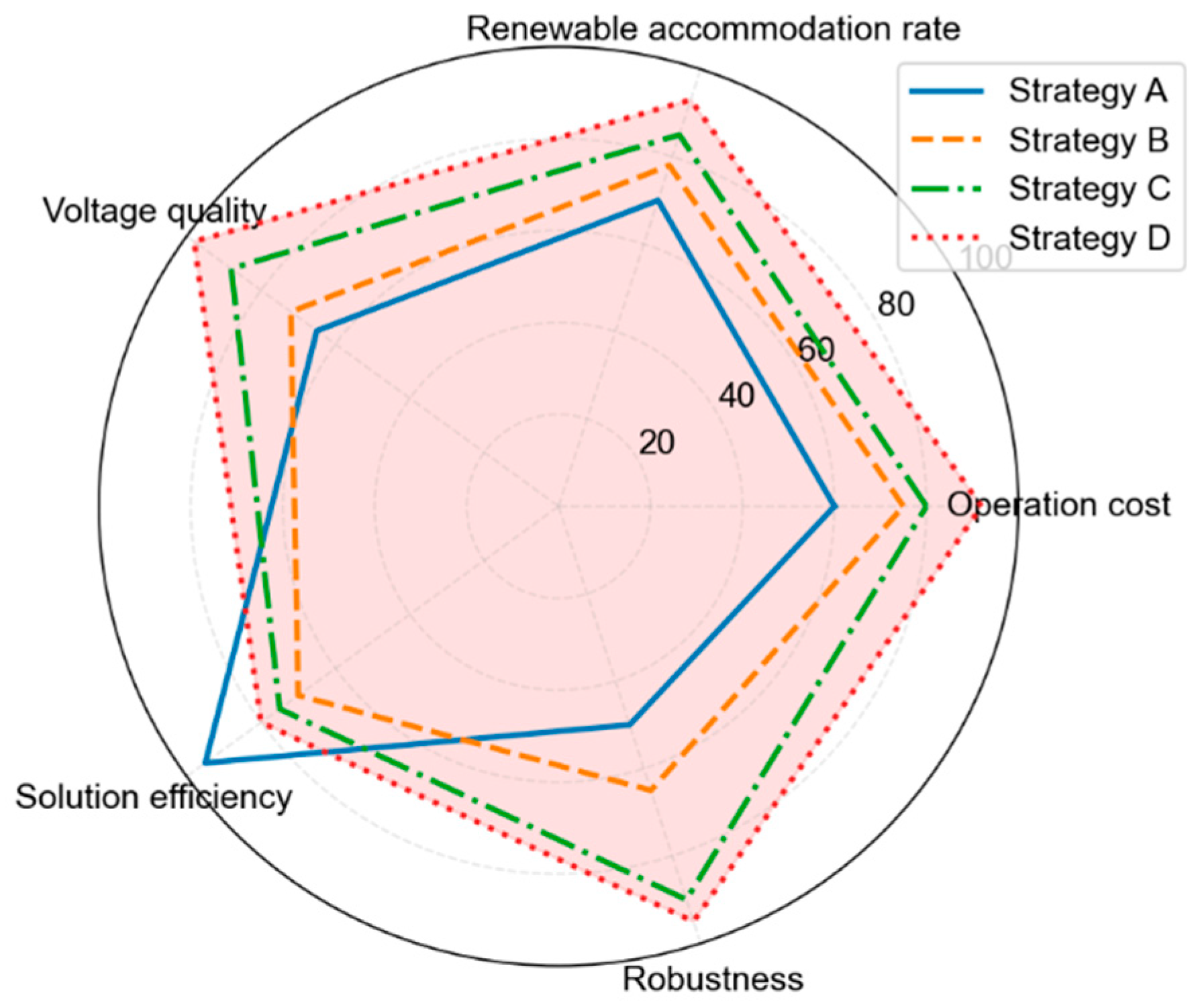
To more intuitively illustrate multidimensional performance differences, Figure 13 presents a comprehensive performance radar chart of four strategies.

Figure 13. Comprehensive performance radar diagram of four scheduling strategies.

Dimension composition: operating cost, renewable energy absorption rate, voltage quality, solution efficiency, and robustness—five dimensions in total. The higher the performance, the better the performance of each strategy.

Strategy A: Highest scores for solving efficiency dimensions, but low in cost, absorption rate, and robustness, causing the overall pattern to shrink noticeably.

Strategy B: Better balance across dimensions than Strategy A, but prominent robustness.

Strategy C: High scores in robustness dimension, but weak economics and solving efficiency.

Strategy D: All five dimensions are on the outermost ring, maximizing graphic coverage and achieving optimal balanced overall performance.

5.4. Robustness Verification Under Complex Operating Conditions

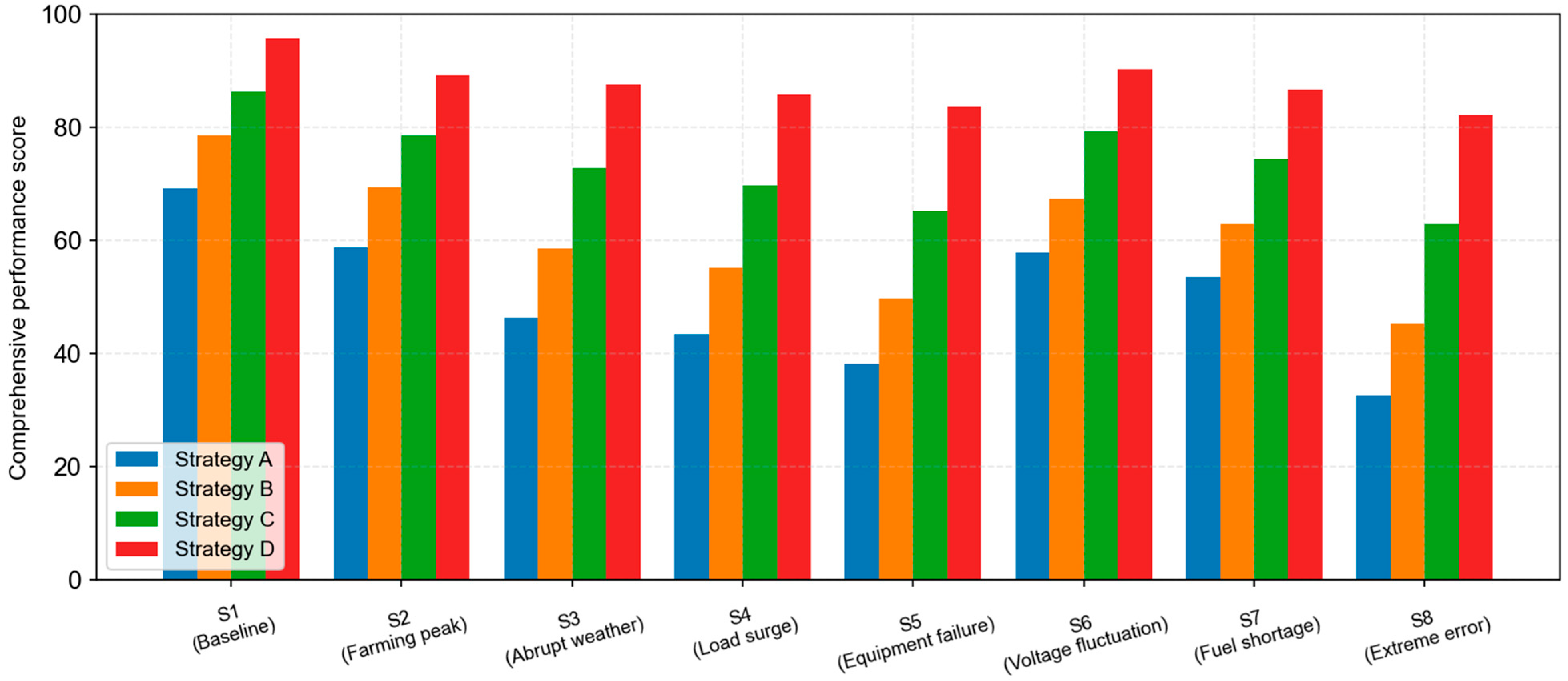
Table 5 compares the comprehensive performance scores of four strategies under eight complex operating conditions (out of 100 points, considering cost, absorption rate, safety, and reliability).

Table 5. Comparison of comprehensive performance under complex working conditions.

Scene Types	Strategy A	Strategy B	Strategy C	Strategy D
S1 (Benchmark)	69.2	78.5	86.3	95.6
S2 (Typical busy farming day)	58.7	69.3	78.5	89.2
S3 (Abrupt extreme weather changes)	46.3	58.6	72.8	87.5
S4 (Workload of busy farming has surged)	43.5	55.2	69.7	85.8
S5 (Equipment failure)	38.2	49.7	65.3	83.6
S6 (Voltage fluctuations)	57.8	67.4	79.2	90.3
S7 (Fuel shortages)	53.6	62.8	74.5	86.7
S8 (Extreme prediction error)	32.7	45.3	62.8	82.1
Average score	50.0	60.9	73.6	87.6

The results show that the proposed method demonstrates optimal robustness under all complex working conditions, with the most significant performance advantage under the extreme prediction-error scenario (S8). This is because the proposed method can dynamically adjust the conservatism of scheduling strategies based on real-time prediction errors, automatically switching to high robustness mode when errors are large [19]. This result is consistent with the findings of reference [11] on robust scheduling of rural high-proportion renewable energy microgrids.

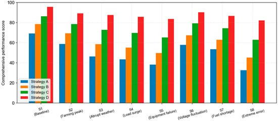
Figure 14 shows a bar comparison chart of the comprehensive scores for the four strategies across the eight scenarios. Horizontal axis: S1~S8, total of eight scenes; longitudinal axis: comprehensive performance score (0~100 points). Each set of scenarios contains four pillars, corresponding to Strategies A, B, C, and D in sequence. Overall pattern: under the benchmark scenario, S1, the differences between strategies are relatively small. In high-disturbance scenarios such as S3, S5, and S8, Strategies A, B, and C showed a cliff-like decline, while Strategy D declined smoothly. In all scenarios, the Strategy D pillar height is significantly higher than the other three, with performance advantages expanding as scenario complexity increases.

Figure 14. Comparison of comprehensive performance scores for each strategy under different complex working conditions.

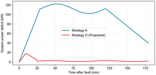
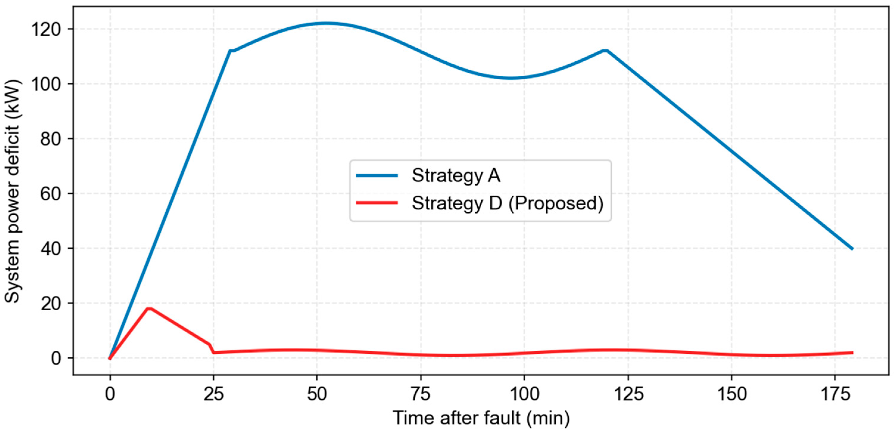
Taking the abrupt extreme weather scenario (S3) as an example, from 12:00 to 15:00, photovoltaic output drops sharply by 40%. Figure 15 shows the system-power deficit curves for Strategy A and Strategy D during this period. Strategy A: After the sharp drop in photovoltaics, the power shortfall will rise rapidly, peaking at 112kW for over 90 min, requiring partial agricultural load cuts to ensure stability. Strategy D: Proactively identify the trend of error expansion, proactively increase unit output and release storage capacity, with a peak power shortage of only 18kW, and balance restored within 15 min, with no load cut-off throughout the process.

Figure 15. System-power deficit comparison curves under extreme weather scenarios.

5.5. Verification of Adaptive Scenario Generation Effectiveness

To verify the effectiveness of the adaptive scenario generation method, the performance of fixed scenarios (10) and adaptive scenarios at different error levels was compared, with results shown in Table 6.

Table 6. Comparison of adaptive scenario generation effects.

Prediction-Error Levels	Fixed Scenarios (10)		Adaptive Scenarios
	Operating Costs (CNY)	Solution Time (s)	Operating Costs (CNY)	Solution Time (s)
5%	12,850	11.2	12,680	12.5
10%	13,120	11.5	12,950	10.3
15%	13,580	11.8	13,240	8.7
20%	14,250	12.1	13,680	7.2
25%	15,120	12.4	14,230	6.5

As shown in Table 6, at the small error level, the adaptive scenario method reduces operating costs by 1.3% compared to fixed scenarios by increasing the number of scenarios. At large error levels, adaptive scenario methods reduce the number of scenarios, shorten the solution time by 47.6% compared to fixed-scenario methods, and reduce operating costs by 5.9%. This fully demonstrates the advantages of adaptive scenario generation methods in balancing computational efficiency and scheduling performance, consistent with the conclusions of the reference.

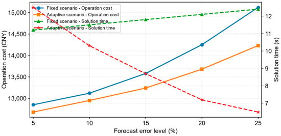
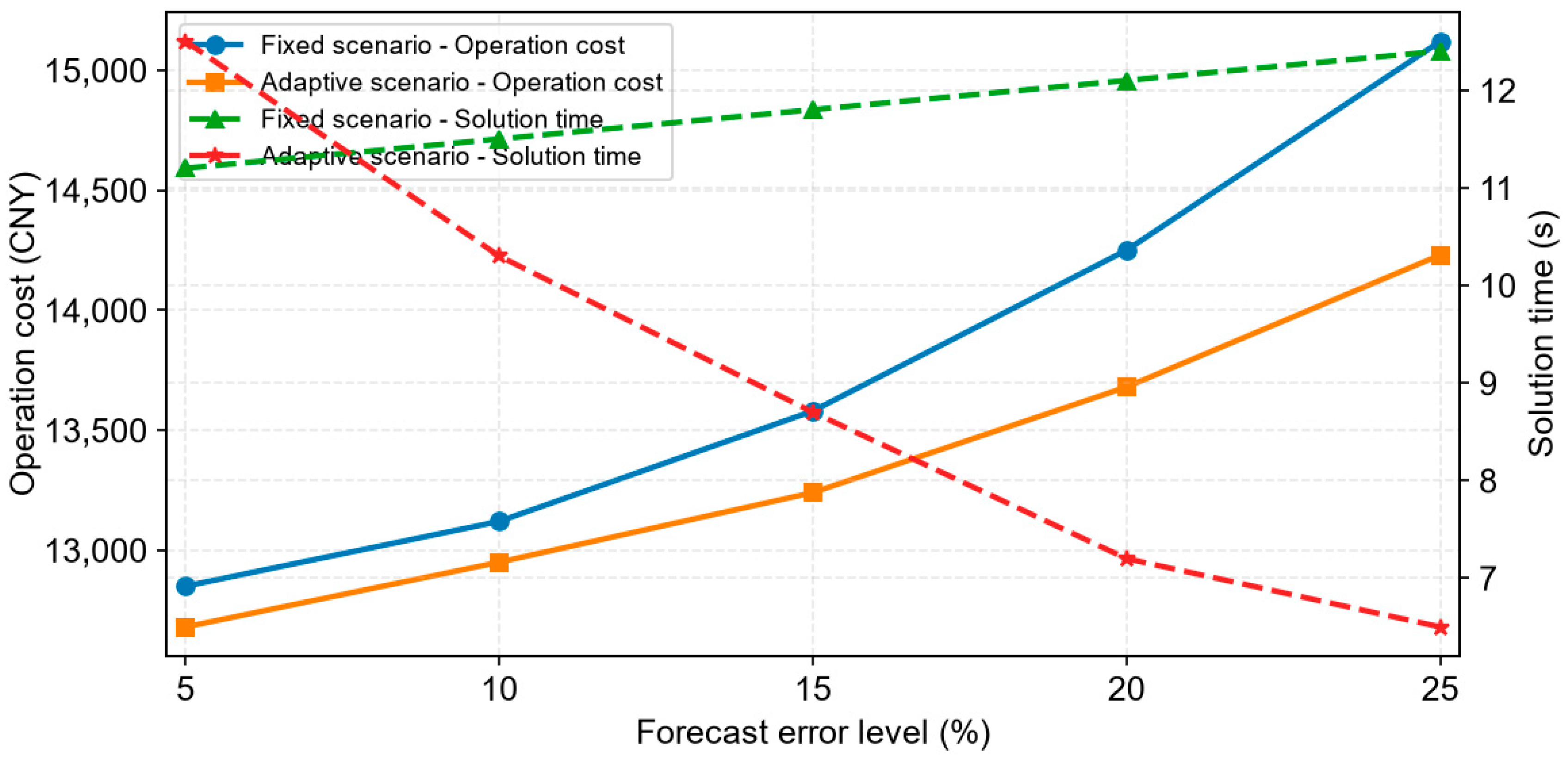
Figure 16 shows the comparison curves of operating costs and solution times for the two scenario generation methods at different error levels. Cost curve: the adaptive scenario is always below the fixed scenario, and the larger the error, the more significant the cost difference; time curve: the solution time for fixed scenarios increases slowly with error, while adaptive scenarios continuously decrease with error, with the greatest advantage at 25% error.

Figure 16. Performance comparison of scenario generation methods under different error levels.

5.6. Predictive-Error Sensitivity Analysis

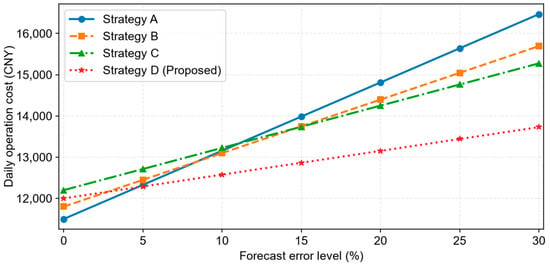
Figure 17 shows the curve of operating costs with the level of forecast error. Strategy A: The slope is the largest; for every 5% increase in error, costs increase by about 7.2%, making it highly sensitive to forecast accuracy. Strategy B: The slope is secondary, and the cost growth is faster than that of robust methods. Strategy C: Flat slope but high benchmark costs. Strategy D: The curve is the smoothest, and when the error increases from 0 to 25%, costs only increase by 12.0%, making it the most resistant to disturbances. Overall, the larger the forecast error, the higher the operating costs for each strategy, but the growth rates differ significantly: Strategy D shows the most moderate cost growth, and when the forecast error reaches 25%, operating costs are 27.3% lower than Strategy A and 9.2% lower than Strategy C.

Figure 17. Sensitivity analysis of operating costs and forecast errors.

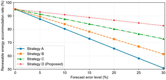
Figure 18 shows the curve of the renewable energy absorption rate with the level of forecast error. As errors increase, traditional strategies are forced to increase wind and solar curtailment to ensure system security, causing the absorption rate to continuously decline: at a 25% error, Strategy A’s absorption rate drops to 58.2% and Strategy C’s to 76.5%; Strategy D, on the other hand, adaptively adjusts its scheduling strategy, prioritizing safety while maximizing renewable energy consumption when errors expand. Even with a 25% error, the absorption rate remains at 84.7%, 26.5 percentage points higher than Strategy A.

Figure 18. Sensitivity analysis of renewable energy absorption rates and forecast errors.

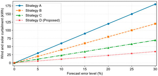
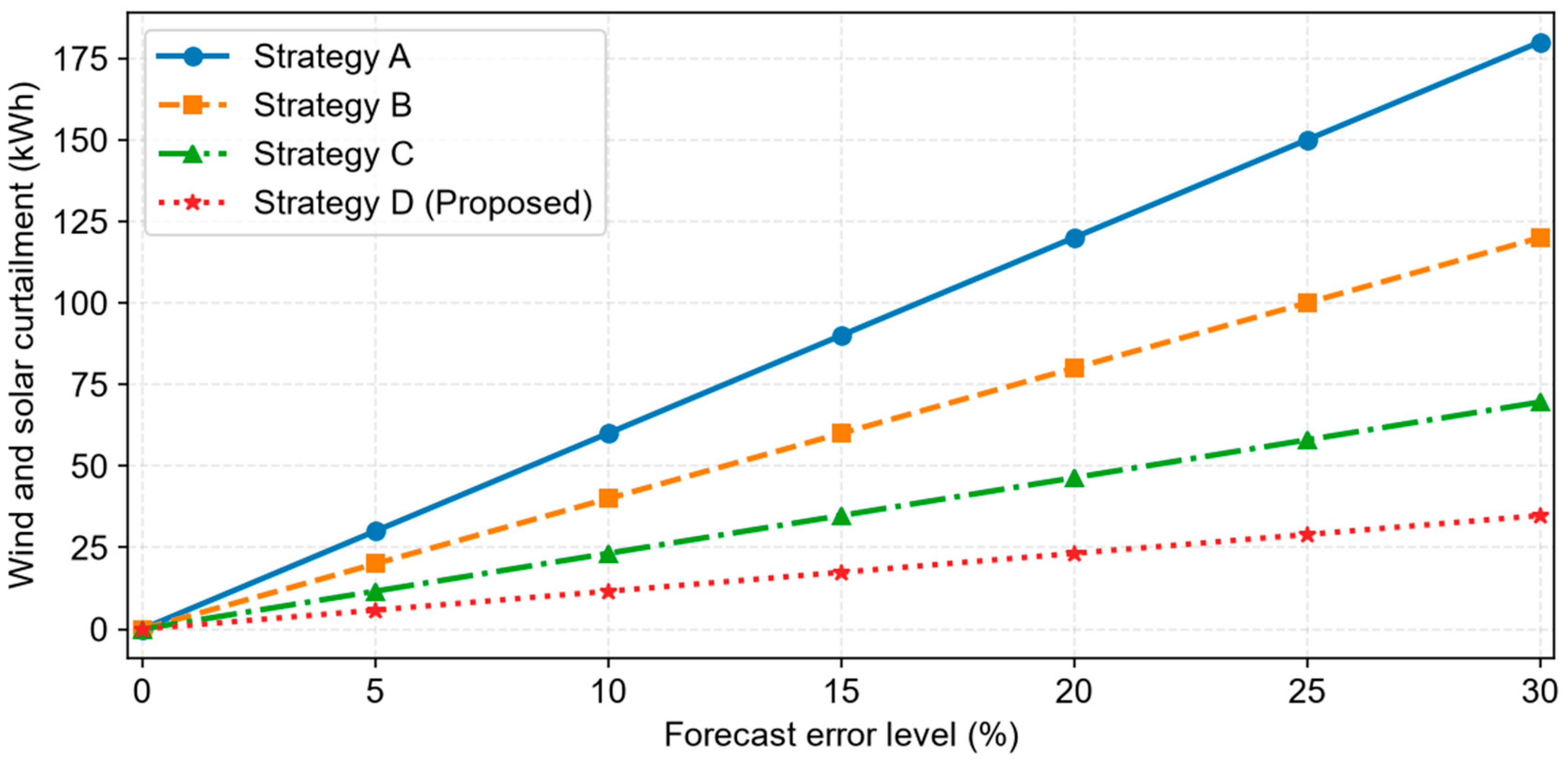
Figure 19 shows the curve of wind and solar power curtailment with the level of forecast error. Within the low-error range, the curtailment amounts for all strategies are at relatively low levels; after errors exceeding 15%, traditional strategies show exponential growth in curtailment, while the growth in this paper is smooth. With a 25% error, Strategy D’s curtailment was only 21.4% of Strategy A’s, fully validating the effect of error-driven scheduling in promoting renewable energy consumption.

Figure 19. Sensitivity analysis of wind and solar power curtailment and prediction errors.

5.7. Full-Process Dynamic-Simulation Closed-Loop Validation

To verify the effect of the full-process dynamic-simulation closed loop, the number of dynamic constraint violations in the method presented in this paper was compared with the presence or absence of simulation closed loops. The results are shown in Table 7.

Table 7. Comparison of closed-loop effects of full-process dynamic simulation.

Scene Types	No Simulated Closed-Loop Simulation	There is a Simulated Closed Loop	Reduction in the Amount
S1 (Benchmark)	2	0	100%
S2 (Typical busy farming day)	4	0	100%
S3 (Abrupt extreme weather changes)	6	0	100%
S4 (Workload of busy farming has surged)	5	0	100%
S5 (Equipment failure)	8	0	100%
S6 (Voltage fluctuations)	3	0	100%
S7 (Fuel shortages)	3	0	100%
S8 (Extreme prediction error)	10	1	90.0%
In total	41	1	97.6%

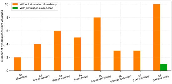
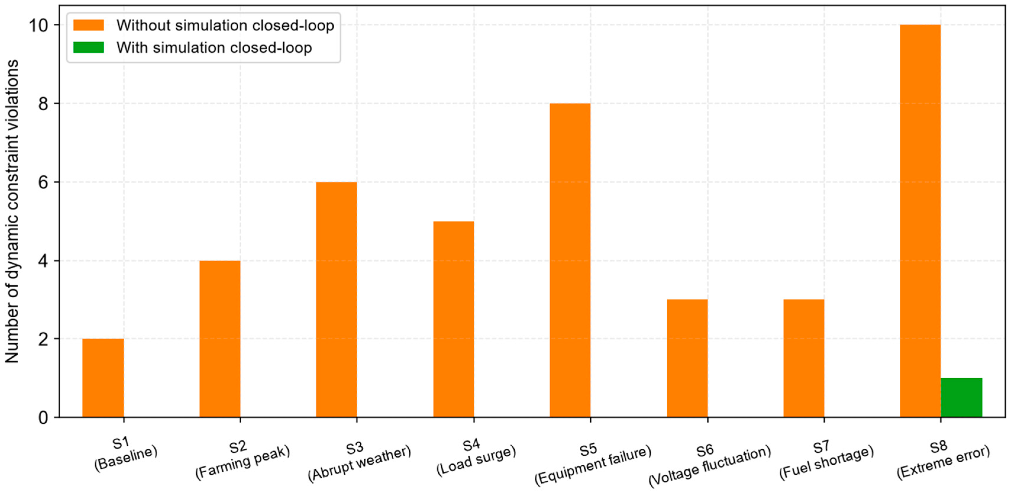
The results show that the full-process dynamic-simulation closed loop reduces the number of dynamic constraint violations by 97.6%, almost eliminating all constraint violations and significantly improving the executability of scheduling strategies and system operational security.

Figure 20 is a bar comparison chart of constraint-violation counts for two types of schemes under eight scenarios, intuitively demonstrating the significant correction effect of the simulation closed loop.

Figure 20. Comparison of the number of dynamic constraint violations with and without simulation closed loops.

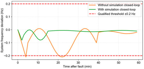
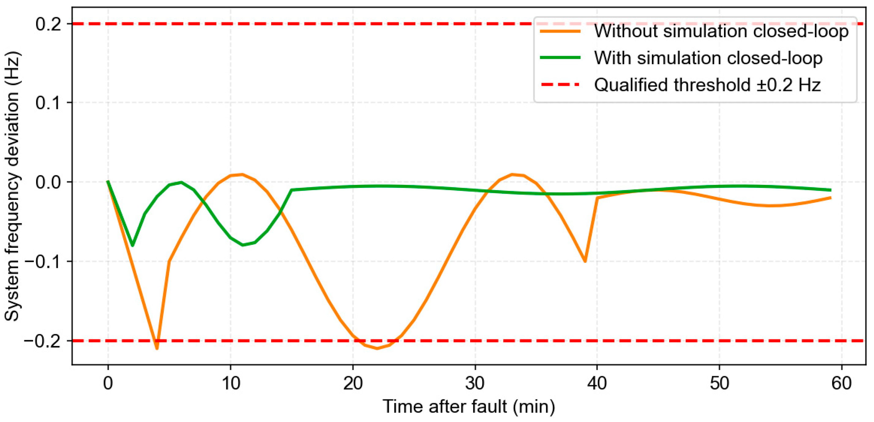
Taking the abrupt extreme weather scenario (S3) as an example, Figure 21 shows the dynamic response curve of system frequency deviation with or without simulated closed-loop simulation. Without simulated closed loops, photovoltaic output drops sharply, causing a rapid frequency drop, with a maximum deviation of 0.21 Hz and multiple oscillations. After introducing a simulation closed loop, the real-time calibration layer quickly adjusts the energy storage output and CHP unit ramp-up rate, with the maximum frequency deviation controlled within 0.08 Hz, the oscillation amplitude significantly reduced, and the system dynamic stability greatly improved.

Figure 21. Comparison curves of system frequency deviation under extreme weather scenarios.

The frequency-deviation trajectories in Figure 21 were obtained by solving the reduced-order SFR model (see Section 3.4) under the power-imbalance sequences generated by different scheduling strategies.

5.8. Full-Lifecycle Economic Benefit Analysis

Based on the full-lifecycle cost theory, the calculation period is 20 years, with a discount rate of 8%. The results are shown in Table 8.

Table 8. Comparison of economic benefits throughout the entire lifecycle.

Economic Indicators	Strategy A	Strategy B	Strategy C	Strategy D
Initial investment (10,000 RMB)	1420.5	1450.8	1475.3	1490.2
Annual operating cost (10,000 RMB)	498.6	462.3	442.7	425.8
Annual maintenance cost (10,000 RMB)	88.7	85.2	82.6	79.5
Present value of total lifecycle cost (10,000 RMB)	7956.3	7425.8	7123.5	6892.7
Internal rate of return (%)	12.1	13.5	14.7	16.0
Payback period (years)	8.9	7.8	7.0	6.1
Efficiency-to-cost ratio	1.34	1.41	1.49	1.60

It should be emphasized that all four compared strategies adopt identical physical hardware capacities for generation, conversion and energy storage equipment in this case study. The higher initial investment of Strategy D (+4.9% compared with Strategy A) does not stem from enlarging the rated power or capacity of power-system hardware. Instead, this incremental capital expenditure covers the extra costs required to deploy the proposed three-layer closed-loop scheduling framework: (1) purchase of industrial edge-computing controllers and high-frequency data-acquisition and real-time communication modules to support multi-time-scale rolling optimization and dynamic-simulation feedback; (2) software development and system-integration costs for adaptive scenario generation, the SOCP optimization wrapper, the dynamic-simulation engine and the forecast-error feedback logic. Even with this moderate one-time upfront increment, Strategy D yields considerable annual savings in operation-and-maintenance expenditure, resulting in a shortened payback period and an improved internal rate of return over the full 20-year lifecycle, which verifies its practical economic attractiveness for real-world rural-site implementation.

Although the initial investment in this method is 4.9% higher than Strategy A, it offers significant economic benefits due to a 14.6% reduction in annual operating costs, a 13.4% reduction in the present value of total lifecycle costs, and a 2.8-year shortening of the payback period, making it suitable for promotion in rural areas [12].

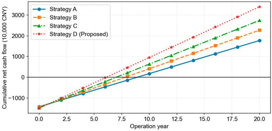
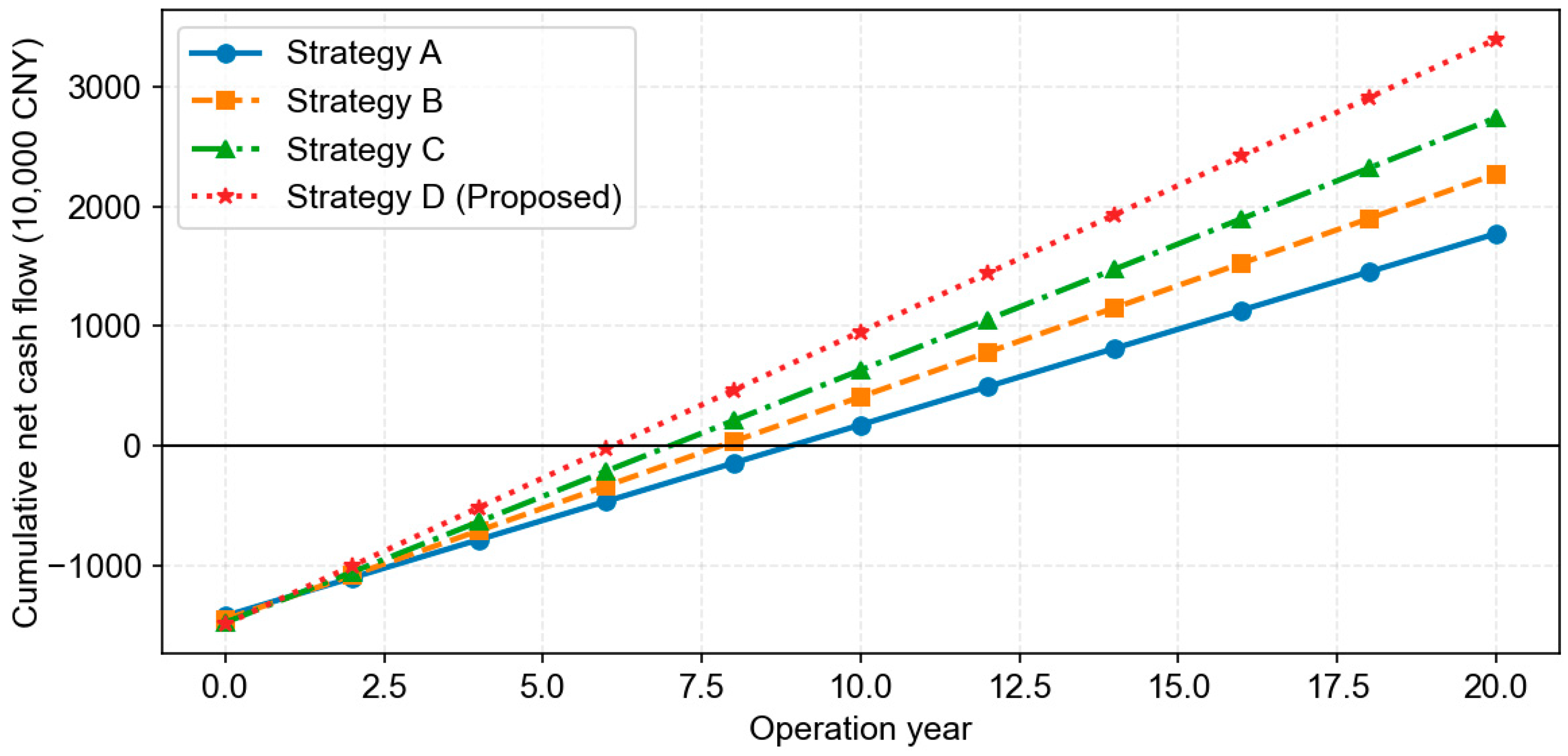
Figure 22 shows the cumulative net cash flow comparison curves for the four strategies. It can be seen that Strategy D, due to a slightly higher initial investment, has a slightly lower initial cash flow than the other strategies, but thanks to lower annual operating costs, its cumulative net cash flow surpasses that of the other strategies in year 6. As the operating years increased, the economic benefit gap continued to widen. Over the 20-year cycle, the cumulative net return exceeded that of Strategy A by 10.636 million yuan, indicating significant long-term value.

Figure 22. Comparison of cumulative net cash flow over the full lifecycle of different strategies.

5.9. Verification of SOCP Relaxation Tightness

To confirm the tightness of the DistFlow second-order cone relaxation, we calculate the relaxation error (ε_ij) for every distribution-network branch under all eight test scenarios (S1-S8). ε_ij is defined in Equation (16). Table 9 lists the maximum, mean, and minimum relaxation errors across all branches for each scenario.

Table 9. Statistics of SOCP relaxation error under different operating scenarios (unit: kW²).

Scenario	Max εij	Mean εij	Min εij
S1 (Benchmark)	0.021	0.007	2.1 × 10−4
S2 (Typical busy farming day)	0.033	0.011	3.3 × 10−4
S3 (Abrupt extreme weather changes)	0.047	0.016	4.7 × 10−4
S4 (Busy-farming-load surge)	0.041	0.013	2.9 × 10−4
S5 (Equipment failure)	0.052	0.018	5.1 × 10−4
S6 (Voltage fluctuations)	0.038	0.012	3.8 × 10−4
S7 (Biomass fuel shortage)	0.027	0.009	2.4 × 10−4
S8 (Extreme prediction error)	0.064	0.022	6.2 × 10−4

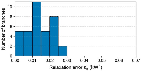
It can be observed from Table 9 that even in the worst-case scenario (S8) with extreme forecast error, the maximum relaxation error is only 0.064 kW². Translated to power magnitude, this gap corresponds to a power deviation far below 0.3 kW, which is negligible for the studied rural integrated-energy-system scale.

Figure 23 presents the branch-wise relaxation-error histogram for Scenario S8 (worst case). Most branches exhibit relaxation errors below 0.03 kW². Only very few branches approach the maximum value of 0.064 kW².

Figure 23. Branch-wise SOCP relaxation-error distribution under Scenario S8.

From the above quantitative results, the second-order cone relaxation is sufficiently tight for this radial rural distribution network. The gap introduced by convex relaxation is numerically insignificant. Therefore, the SOCP-solved optimal points satisfy the original DistFlow equality constraints with high accuracy, and the obtained scheduling solutions are physically valid [20].

6. Conclusions and Outlook

This paper proposes a forecast-error-driven three-layer multi-time-scale robust-scenario hybrid scheduling framework for rural integrated energy systems (RIESs). Based on multi-year field-measured data of rural energy systems, the multi-temporal statistical characteristics of multi-source forecast errors are revealed. An adaptive scenario generation method and robust-constraint adjustment mechanism is developed, and a full-process “forecast–optimization–simulation” closed-loop control architecture is constructed. Improved second-order cone programming (SOCP) is adopted to solve the established optimization model. The main quantitative findings are summarized as follows:

• Compared with traditional deterministic scheduling (Strategy A), the proposed method reduces the daily operating cost by 12.8%, raises the renewable energy accommodation rate by 22.6%, cuts carbon emissions by 29.1%, and restrains the dynamic constraint-violation rate below 0.05%.
• Benefiting from the full-process dynamic-simulation closed-loop mechanism, dynamic constraint violations are reduced by 97.6%, significantly improving the physical executability of scheduling instructions.
• The adaptive strategy dynamically adjusts scenario quantity and robust conservatism according to real-time forecast-error quantiles. Under ±25% forecast-error disturbance, the approach maintains stable system performance with an average solution time within 9 s, satisfying the computation requirement of rural edge-computing hardware.
• From the full-lifecycle economic perspective, although Strategy D requires moderate additional upfront investment for edge-computing hardware and closed-loop scheduling software (without increasing power-equipment hardware size), the payback period is shortened to 6.1 years, and the internal rate of return reaches 16.0%, showing favorable economic competitiveness for rural deployment.

The main merits of this work lie in three aspects. First, it avoids the inherent drawbacks of conventional static scheduling: excessive conservatism under small forecast errors and insufficient safety under large disturbances. Second, the three-layer closed-loop architecture bridges the gap between theoretical optimization solutions and practical physical operation via dynamic-simulation feedback. Third, the SOCP-based solution achieves a good trade-off among robustness, economic benefit and computational efficiency, which is especially suitable for rural scenarios featured with weak power grids, prominent source-load uncertainties and limited computing resources.

The presented scheduling strategy can be practically applied to real-world rural multi-energy stations, village-level integrated energy projects, and agricultural microgrids with high shares of wind–solar distributed generation. It can provide decision support for field operation dispatch, edge-controller algorithm deployment, and rural energy planning.

For future research aligned with industry development trends, three promising directions are suggested:

(1)

Develop distributed collaborative scheduling algorithms for clustered multi-microgrids under spatial–temporal correlated forecast errors.

(2)

Integrate deep-learning-based ultra-short-term forecast correction to further improve the adaptability toward extreme meteorological and agricultural load disturbances.

(3)

Introduce carbon-trading mechanisms and flexible agricultural demand-response resources to realize low-carbon-oriented robust optimal scheduling for rural integrated energy systems.

References

- Ye, L.; Liu, Z.; Liang, Y. Development path of a modern rural power grid under dual carbon target based on data analysis. Int. J. Low.-Carbon Technol. 2024, 19, 217–226. [Google Scholar] [CrossRef] [Scilit]
- Kushwaha, K.P.; Jha, K.R.; Bhattacharjee, C.; Verma, H.K. Integrated Load–Source Side Management for Techno-Economic-Environmental Performance Improvement of the Hybrid Renewable Energy System for Rural Electrification. Electr. Power Compon. Syst. 2025, 53, 2164–2186. [Google Scholar] [CrossRef] [Scilit]
- Zhang, H.; Yang, Z.; Jin, Y.; Lin, F.; Mi, J. An identifiability-guided dual-mode current-conditioned equivalent circuit model for supercapacitors in urban rail transit energy storage systems. J. Energy Storage 2026, 182, 124786. [Google Scholar] [CrossRef] [Scilit]
- Li, J.; He, Y.; Wu, W.; Li, S.; Zhao, Z.; Zhang, X.; Zhang, Y.; Xiang, W. Capacity optimization of rural residential distributed photovoltaic-Battery energy storage system considering uncertainties. J. Energy Storage 2026, 148, 120246. [Google Scholar] [CrossRef] [Scilit]
- Zhang, S.; Ding, S.; Li, Y.; Wei, M.; Tan, Q. A bi-level planning model of integrated energy capacity configuration for data center cluster considering computing-electricity coupling operation and supply-demand uncertainties. Appl. Energy 2026, 425, 128499. [Google Scholar] [CrossRef] [Scilit]
- Li, J.; Zhang, Z.; Liang, C.; Zeng, F. Multi-objective robustness of integrated energy system considering source-load uncertainty. J. Shanghai Jiao Tong Univ. 2025, 59, 175–185. [Google Scholar]
- Li, D.; Li, X.; Cao, B.; Zhu, Y.; Xu, L.; Chen, K.; Yan, L.; Ren, J. Multi-timescale spot market-oriented dispatch strategy of hierarchical flexibility resources for park integrated energy systems. Processes 2026, 14, 756. [Google Scholar] [CrossRef] [Scilit]
- Cui, J.; Wei, J.; Liu, H.; Zhang, X.; Li, C.; Li, Y. Dynamic economic assessment of thermal power and energy storage in integrated energy markets using an adaptive decision framework. J. Energy Storage 2026, 167, 122554. [Google Scholar] [CrossRef] [Scilit]
- Ishraque, M.F.; Shezan, S.A.; Ali, M.M.; Rashid, M. Optimization of load dispatch strategies for an islanded microgrid connected with renewable energy sources. Appl. Energy 2021, 292, 116879. [Google Scholar] [CrossRef] [Scilit]
- Mao, Y.; Jiao, X. Flexible batch loads as “virtual batteries”: Distributionally robust optimization for computation-electricity co-scheduling in data center integrated energy system. Electr. Eng. 2026, 108, 246. [Google Scholar] [CrossRef] [Scilit]
- Yang, S.; Guo, N.; Zhang, S. Robust optimal scheduling of agricultural microgrid combined with irrigation system under uncertainty conditions. J. Shanghai Jiao Tong Univ. 2024, 58, 1432–1442. [Google Scholar]
- Guo, L.; Xu, X.; Lv, F. Forecasting–scheduling co-optimization for rural microgrids: An edge-deployable approach. Energies 2026, 19, 1910. [Google Scholar] [CrossRef] [Scilit]
- Phan, V.T.; Truong, H.B.H.; Pham, P.V.; Cho, N.; Kim, D. A multi-objective approach for integrated energy hub with waste incineration plants integrating carbon capture technology, and electric vehicle parking lots under uncertainties. Sustain. Energy Grids Netw. 2026, 45, 102121. [Google Scholar] [CrossRef] [Scilit]
- Bermúdez, G.J.; Rózsai, M.; Salvucci, R.; Jaxa-Rozen, M.; Sikora, P.; Wegener, M.; Aycart, J.; Neuwahl, F. Modelling the power sector with high time resolution in the integrated energy system model POTEnCIA: Capturing the value of flexibility in high renewable share power systems. Energy Rep. 2026, 16, 109457. [Google Scholar] [CrossRef] [Scilit]
- Meng, Q.; Zhao, L.; She, Q.; Guo, Q.; Guo, L.; Chen, P.; Zhao, J.; Yao, W.; Gao, Y.; Wang, S.; et al. Generation–grid–load–storage coordination for a park-level integrated energy microgrid under new-type power systems. Energy Rep. 2026, 15, 108924. [Google Scholar] [CrossRef] [Scilit]
- Mi, J.; Su, J.; Xue, Y.; Chang, X.; Li, Z.; Sun, H. Energy circuit theory-enabled quasi-dynamic security assessment for integrated electricity-gas energy system. Energy Convers. Manag. 2026, 363, 121673. [Google Scholar] [CrossRef] [Scilit]
- Shi, T.; Huang, R.; Yin, H. Research on energy management strategy of integrated energy system. In Proceedings of the 2020 Asia-Pacific Conference on Power and Electrical Engineering (ACPEE), Chengdu, China, 4–7 June 2020. [Google Scholar] [CrossRef] [Scilit]
- Zhang, W.; Qiao, G.; Li, Y. Low-carbon optimization scheduling strategy for integrated energy system considering gas and thermal inertia. J. Comput. Sci. Electr. Eng. 2026, 8, 48–56. [Google Scholar] [CrossRef] [Scilit]
- Xiao, H.; Long, F.; Zeng, L.; Zhao, W.; Wang, J.; Li, Y. Optimal scheduling of regional integrated energy system considering multiple uncertainties and integrated demand response. Electr. Power Syst. Res. 2023, 221, 108213. [Google Scholar] [CrossRef] [Scilit]
- Li, Z.; Wang, Y.; Si, Y.; Gao, X. Price-Calibrated Network Loss–Carbon Emission Co-Optimization for Radial Active Distribution Networks via DistFlow-Based MISOCP Reconfiguration. Sustainability 2026, 18, 544. [Google Scholar] [CrossRef] [Scilit]
Disclaimer/Publisher’s Note: The statements, opinions and data contained in all publications are solely those of the individual author(s) and contributor(s) and not of MDPI and/or the editor(s). MDPI and/or the editor(s) disclaim responsibility for any injury to people or property resulting from any ideas, methods, instructions or products referred to in the content. |
© 2026 by the authors. Licensee MDPI, Basel, Switzerland. This article is an open access article distributed under the terms and conditions of the Creative Commons Attribution (CC BY) license.