A Cloud–Edge Collaborative Multi-Parameter Fusion Approach for Adaptive Early Warning and Condition Assessment of Production Control Systems

Abstract

To address the limitations of traditional fixed-threshold alarms for distributed control systems (DCS), programmable logic controllers (PLC), safety instrumented systems (SIS), and remote terminal unit (RTU) production control systems in oil-gas stations, which suffer from delayed response, binary-only outputs, and an inability to characterize the continuous degradation process of equipment, this paper proposes a cloud–edge collaborative, human-reviewed adaptive diagnosis and early-warning algorithm for production control systems under a cloud–edge collaborative architecture integrating deterministic rules and multi-parameter fusion. Here, adaptive denotes cloud-assisted, human-reviewed parameter updating rather than autonomous online learning. A lightweight rule engine and risk fusion model are deployed at the edge side. Monitoring points are classified into nine risk groups according to functional semantics, and heterogeneous measurements are normalized into dimensionless risk scores within the range of [0, 1] through linear and binary mappings. A hierarchical judgment logic is designed to distinguish critical hard faults (e.g., communication and power supply failures) from ordinary parameter threshold-exceedance warnings, enabling precise point-level traceability. A three-stage fusion model is established. By introducing the pressure term, exponential smoothing filter and hysteresis latch, it generates a continuous condition-assessment score ranging from 0 to 100. The cloud side is responsible for threshold parameter management, global condition analysis across multiple stations, and iterative update of the fault knowledge base, forming a collaborative closed-loop of “real-time diagnosis at the edge and continuous optimization in the cloud”. Tests are conducted using seven-day time-series data from five PLC devices. A total of 3358 threshold-exceedance events are identified, and the proportion of continuous-variable anomalies ranges from 7.08% to 7.34%. Most exceedance events are one-minute transient pulses, and the temporal overlap coefficient between state-variable anomalies and continuous-variable anomalies reaches 0.61. Hard faults can forcibly constrain the condition-assessment interval, while fine-grained load differentiation can be realized under normal operating conditions. Ablation experiments verify the benefits of the three optimization mechanisms for interval constraint, stable output and hysteretic fault recovery.

1. Introduction

In recent years, with the in-depth advancement of Industry 4.0 and the comprehensive acceleration of smart oilfield construction, digital transformation has become essential for the oil and gas industry to improve production efficiency and ensure operational safety. Production control systems such as DCS, PLC, and SIS serve as the core infrastructure for production control and safety protection at oil and gas stations, undertaking key functions such as full-process continuous production scheduling and safety interlocking under hazardous operating conditions. Their operational stability directly determines the production efficiency and intrinsic safety level of oil and gas production. Oil and gas production features uninterrupted technological workflows, flammable and explosive operating environments, high temperature and pressure, widely distributed station equipment, and drastically fluctuating operating conditions. Faults in production control systems generally evolve through subtle performance degradation, sustained trend deterioration, fault triggering, and short-term recovery, while strong multivariable coupling and industrial noise greatly increase the difficulty of fault identification and risk prediction.

Early fault diagnosis for production control systems and process-industry equipment relied mainly on expert rules, fixed-threshold alarms, fault-tree analysis, principal component analysis (PCA), partial least squares (PLS), and support vector machines (SVM). These methods are relatively interpretable and straightforward to implement, but they have limited capability in identifying complex nonlinear operating conditions, noise disturbances, multivariable coupled faults, and weak incipient anomalies [1,2,3]. In recent years, with the accumulation of self-diagnostic data from the Industrial Internet of Things and supervisory control and data acquisition (SCADA), distributed control system (DCS), programmable logic controller (PLC), and safety instrumented system (SIS) platforms, data-driven fault diagnosis and predictive maintenance have become research hotspots. Zhao et al. [4] systematically summarized the applications of deep-learning models in machine health monitoring, pointing out that autoencoders, deep belief networks, convolutional neural networks (CNNs), and recurrent neural networks (RNNs) have become important research directions. Overall, domestic and international studies have formed a basic technical pipeline of signal preprocessing, feature extraction, fault classification, condition assessment, and remaining-useful-life prediction. However, most achievements still focus on single equipment or mechanical components, while module-level, channel-level, communication-level, and safety-loop-level fault diagnosis for production control systems such as DCS, PLC, and SIS at oil and gas production sites remains relatively insufficient.

Oil and gas production sites feature strong production continuity, widely distributed equipment, high-risk environments, large operating-condition fluctuations, and complex communication conditions. Traditional periodic inspection and corrective maintenance can hardly meet the requirements of high reliability, low downtime, and safe production. At the same time, the maturing edge computing and deep-learning algorithms make it possible to perform real-time processing and efficient inference of massive time-series data near the data source, fundamentally breaking the traditional constraints of computing power and communication bandwidth. In recent years, foreign oil and gas industries have gradually applied artificial intelligence (AI), the Internet of Things, edge computing, and predictive maintenance to drilling platforms, oil wells, pumping stations, compressors, offshore platforms, and pipeline systems. Focusing on condition prediction of physical assets in the oil and gas industry, Figueroa Barraza et al. [5] studied a deep-learning-based condition-prediction method and emphasized that asset degradation modeling based on historical operating data, fault records, and sensor data can support maintenance decisions and risk control for high-value equipment. For oil-well anomaly detection, Silva et al. [6] used one-class classifiers, anomaly-detection models, and data resampling strategies to identify undesired production events, indicating that unsupervised or semi-supervised learning methods are more suitable for early anomaly detection when fault samples are scarce and anomaly types are imbalanced. Latrach [7] compared the applicability of fully connected neural networks, CNNs, and RNNs to the NASA C-MAPSS dataset, bearing datasets, and key oilfield equipment, and combined PCA, Fourier analysis, and wavelet analysis for feature enhancement, providing a technical reference for remaining-useful-life prediction and condition recognition of key oilfield equipment. In China, Zhang Laibin and Wang Jinjiang [8] emphasized the integration of the industrial Internet, condition monitoring, fault prediction, remote diagnosis, and maintenance decision-making, and proposed edge acquisition, industrial gateways, data governance, model analysis, and visualization platforms to support full-lifecycle operation and maintenance of oil and gas storage and transportation equipment. Similarly, Zhang Xuhui et al. [9] constructed a digital-twin-based predictive maintenance system for complex mining equipment, using condition monitoring, three-dimensional visualization, optimized BP neural networks, and database linkage to realize early warning of faults in key components. Although it targets mining equipment, its architecture of physical equipment, data acquisition, virtual mapping, intelligent diagnosis, and maintenance strategy provides a useful reference for intelligent operation and maintenance of oil and gas station equipment. From the perspective of technical trends, edge computing has become an important support for the deployment of AI diagnosis at oil and gas sites. On the one hand, the edge side can complete data access, cleaning, denoising, compression, and preliminary inference for industrial protocol data such as OPC UA, Modbus, Profinet, and Highway Addressable Remote Transducer (HART), reducing cloud transmission pressure. On the other hand, the cloud side can perform model training, knowledge-base updating, global condition assessment, and cross-station model transfer, forming a cloud–edge collaborative closed loop. However, existing research generally focuses on predictive maintenance of mechanical equipment and production assets, and the utilization of native self-diagnostic data of production control systems remains insufficient. In particular, there is still obvious room for improvement in the fusion diagnosis and quantitative condition assessment of multi-dimensional data, including PLC module status, DCS redundancy switching logs, SIS safety-loop integrity, control-network communication quality, input/output (I/O) channel drift, firmware anomalies, and controller load [10,11,12,13].

Production control systems at oil and gas production sites are not only production control systems but also safety assurance systems. Their fault diagnosis and condition prediction need to simultaneously satisfy real-time performance, reliability, interpretability, and cybersecurity requirements. In recent years, research on industrial AI fault diagnosis has begun to focus on multi-source information fusion and relational modeling in complex interconnected systems. In a 2025 review, Nti et al. [14] pointed out that in complex industrial systems, relying solely on a single sensor or a single variable makes it difficult to accurately determine fault propagation paths, and integrating sensor outputs, environmental variables, maintenance records, and system topology can improve fault localization and predictive maintenance. Singh et al. [15] also pointed out in a roadmap study on machine-learning fault diagnosis that deep learning bridges the gap between large-scale industrial monitoring data and condition recognition, while challenges remain in few-shot faults, cross-condition transfer, model interpretability, online learning, and real-time deployment. In the field of complex industrial system diagnosis in China, Luo Hao et al. [16] emphasized combining operating data, mechanistic knowledge, control logic, and safety constraints to form a framework for fault detection, diagnosis, fault-tolerant control, and safety control oriented to complex industrial processes.

In summary, most existing research on fault diagnosis and equipment condition assessment focuses on vibration signals of rotating machinery and general deep learning modeling. For the native structured self-diagnostic data of DCS, PLC, SIS, and RTU production control equipment at oil and gas stations, the current modeling system still has obvious shortcomings: it cannot distinguish the alarm priority between safety-critical points such as communication and power supply and conventional monitoring points; it lacks a hierarchical alarm mechanism for hard faults and ordinary parameter threshold exceedance; and it cannot output refined continuous condition indicators to characterize the gradual degradation of equipment from normal operation to failure. Moreover, most data-driven models have high training costs and are difficult to deploy on edge gateways with low computing power. To address the above research gaps, this paper proposes an early-warning and condition-assessment algorithm. Based on the physical functional semantics of monitoring points, the method divides all measuring points into nine risk groups. Segmented linear risk mapping and binarization mapping are designed for continuous variables and state variables, respectively, so that heterogeneous measuring points with different dimensions and encoding formats are uniformly converted into dimensionless risk scores within [0, 1]. Through a hierarchical deterministic rule-judgment architecture, it immediately intercepts two types of hard faults, namely safety-critical hardware failures and parameters reaching physical limits, distinguishes ordinary threshold-exceedance warnings, and synchronously outputs point-level traceability information. Furthermore, a three-stage fusion framework of risk-group score, comprehensive fault degree, and condition-assessment mapping is constructed. By introducing the operating pressure term, exponential smoothing, and recovery hysteresis, a continuous condition-assessment score from 0 to 100 is generated, providing comprehensive support for hierarchical alarming and long-term quantitative monitoring of equipment operating status.

2. Overall Architecture for Cloud–Edge Collaborative Fault Diagnosis

2.1. Division of Cloud and Edge Tasks

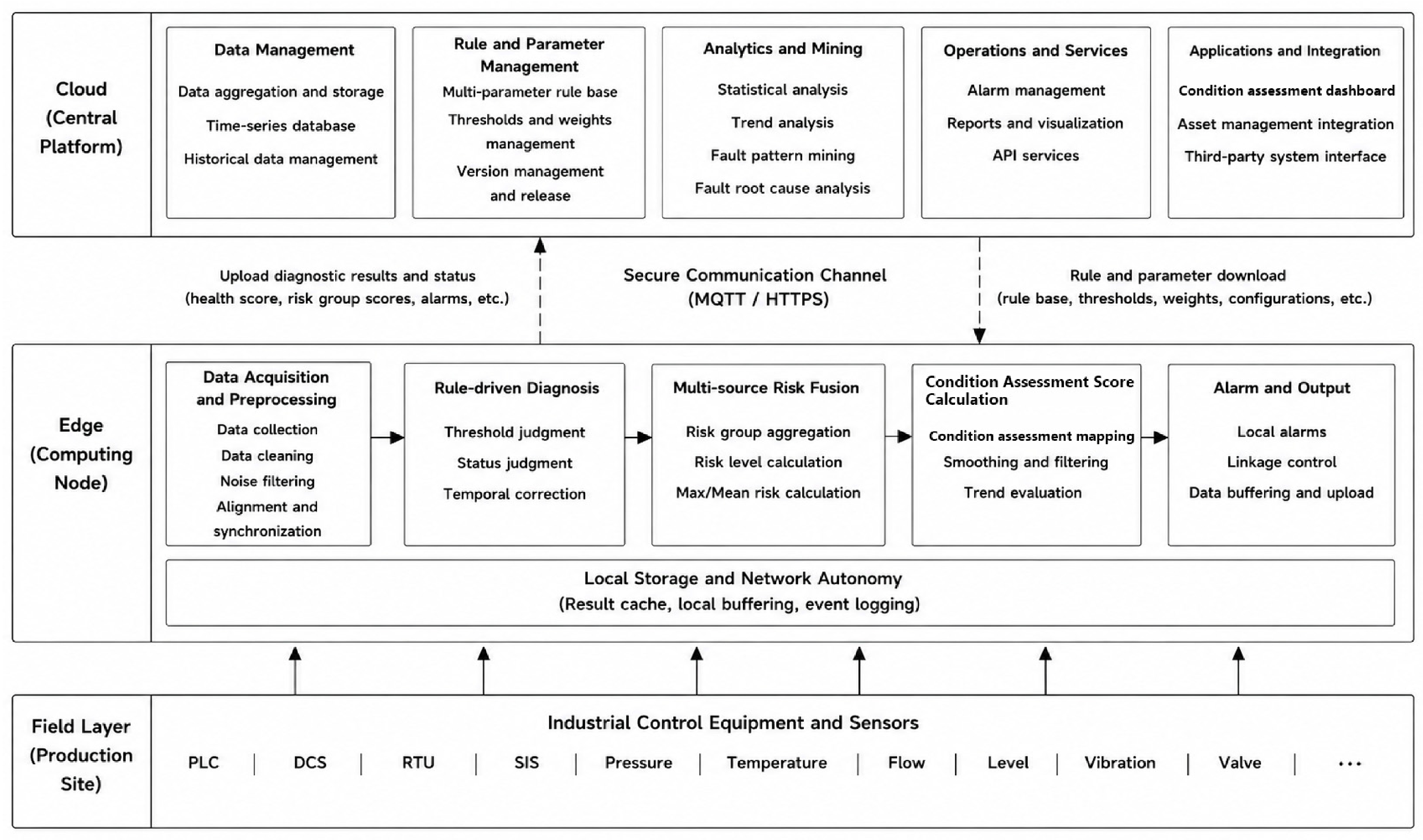
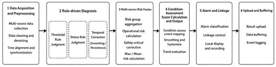
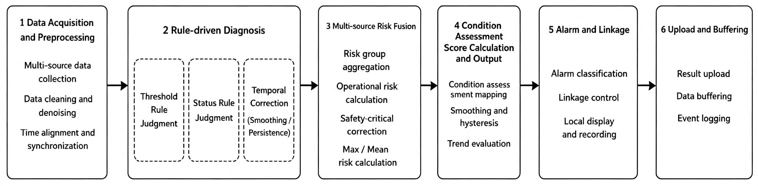
To meet engineering demands [17,18] for low latency, high reliability, weak network dependency, and centralized management, this paper proposes a cloud–edge collaborative deployment architecture that splits the adaptive early-warning and diagnosis into real-time edge computing and global cloud management. The overall architecture is shown in Figure 1.

Figure 1. Overall cloud–edge collaborative fault-diagnosis architecture for oil and gas production control systems.

2.2. Real-Time Edge-Side Diagnostic Procedure

The core edge-side algorithm is illustrated in Figure 2. The edge node sequentially performs point-data acquisition, heterogeneous risk mapping, risk-group aggregation, hierarchical rule-based diagnosis, multi-parameter fusion, and temporal optimization of the condition assessment. It outputs local alarms, abnormal points, and summarized results for cloud aggregation.

Figure 2. Adaptive edge-side diagnosis and early-warning workflow driven by a multi-parameter rule base.

Assume that, at time t, the edge node receives the following set of raw device points:

$$\mathrm{X}\left(\mathrm{t}\right)=\{{\mathrm{x}}_1\left(\mathrm{t}\right),{\mathrm{x}}_2\left(\mathrm{t}\right),\dots ,{\mathrm{x}}_{\mathrm{m}}\left(\mathrm{t}\right)\}$$

(1)

The edge side first completes point type identification, missing value processing, timestamp verification and dimension inspection according to the point configuration table, then maps continuous variables and state variables to unified risk scores ${\mathrm{r}}_{\mathrm{j}}\left(\mathrm{t}\right)\in \left[0, 1\right]$. On this basis, the edge rule engine invokes the multi-parameter rule base to preferentially detect safety-critical anomalies such as communication failure, power supply fault and physical limit crossing. If no hard fault is triggered, further detection of ordinary state anomalies and continuous variable threshold out-of-limit events is carried out. The multi-parameter fusion module calculates risk group scores, comprehensive fault degree and raw condition assessment, and then generates the final condition assessment via operation pressure terms, exponential smoothing and recovery hysteresis mechanisms.

The structured edge-side output is defined as follows:

$$\mathrm{E}\left(\mathrm{t}\right)=\left\{\mathrm{d},\mathrm{t},{\mathrm{y}}_{\mathrm{h}\mathrm{a}\mathrm{r}\mathrm{d}}\left(\mathrm{t}\right),{\mathrm{y}}_{\mathrm{l}\mathrm{i}\mathrm{m}\mathrm{i}\mathrm{t}}\left(\mathrm{t}\right),\tilde{\mathrm{H}}\left(\mathrm{t}\right),\mathrm{R}\left(\mathrm{t}\right),\mathsf{\Omega }\left(\mathrm{t}\right)\right\}$$

(2)

where $\mathrm{d}$ denotes the device identifier, ${\mathrm{y}}_{\mathrm{h}\mathrm{a}\mathrm{r}\mathrm{d}}\left(\mathrm{t}\right)$ the hard fault flag, ${\mathrm{y}}_{\mathrm{l}\mathrm{i}\mathrm{m}\mathrm{i}\mathrm{t}}\left(\mathrm{t}\right)$ the ordinary limit-violation flag, $\tilde{\mathrm{H}}\left(\mathrm{t}\right)$ the final condition assessment, $\mathrm{R}\left(\mathrm{t}\right)$ the risk group score vector, and $\mathsf{\Omega }\left(\mathrm{t}\right)$ the set of anomaly points.

2.3. Centralized Cloud Management and Parameter Coordination

The cloud maintains the multi-parameter rule base and the unified parameter set required for edge diagnosis. Rather than consisting of isolated rules, the rule base provides a structured organization of deterministic rules, parameters, priorities, scopes of application, and version information. Its basic form can be expressed as follows:

$$\mathcal{K}={\left\{{\mathrm{R}}_{\mathrm{i}},{\mathsf{\Theta }}_{\mathrm{i}},{\mathrm{P}}_{\mathrm{i}},{\mathrm{C}}_{\mathrm{i}},{\mathrm{V}}_{\mathrm{i}}\right\}}_{\mathrm{i}=1}^{\mathrm{N}}$$

(3)

where ${\mathrm{R}}_{\mathrm{i}}$ denotes the $\mathrm{i}-\mathrm{t}\mathrm{h}$ deterministic rule, ${\mathsf{\Theta }}_{\mathrm{i}}$ the rule parameters, ${\mathrm{P}}_{\mathrm{i}}$ the execution priority, ${\mathrm{C}}_{\mathrm{i}}$ the applicable devices and triggering conditions, and ${\mathrm{V}}_{\mathrm{i}}$ the rule version. Based on their functions, the rule base can be divided into the following rule sub-bases: the point semantic rule sub-base, the graded threshold rule sub-base, the safety-critical state rule sub-base, the risk fusion rule sub-base, and the condition assessment temporal correction rule sub-base.The composition of the multi-parameter rule base is summarized in Table 1.

Table 1. Composition of the multi-parameter rule base.

Rule Sub-Base	Main Parameters	Function
Point semantic rule sub-base	Point ID, data type, normal-state code, unit, and risk group	Unifies point semantics across devices from different vendors
Graded threshold rule sub-base	Normal upper bound, warning threshold, fault onset, and physical limit	Supports piecewise risk mapping and limit-violation detection for continuous quantities
Safety-critical state rule sub-base	Communication, power supply, program status, and safety-critical flag	Enables prioritized interception of hard faults
Risk fusion rule sub-base	Group weight, maximum coefficient, mean coefficient, and anomaly density coefficient	Calculates risk group scores and the composite fault degree
Condition assessment temporal correction rule sub-base	Smoothing coefficient, persistence period, and recovery hysteresis period	Suppresses transient fluctuations and controls condition assessment recovery

Table 1. Composition of the multi-parameter rule base.

Rule Sub-Base	Main Parameters	Function
Point semantic rule sub-base	Point ID, data type, normal-state code, unit, and risk group	Unifies point semantics across devices from different vendors
Graded threshold rule sub-base	Normal upper bound, warning threshold, fault onset, and physical limit	Supports piecewise risk mapping and limit-violation detection for continuous quantities
Safety-critical state rule sub-base	Communication, power supply, program status, and safety-critical flag	Enables prioritized interception of hard faults
Risk fusion rule sub-base	Group weight, maximum coefficient, mean coefficient, and anomaly density coefficient	Calculates risk group scores and the composite fault degree
Condition assessment temporal correction rule sub-base	Smoothing coefficient, persistence period, and recovery hysteresis period	Suppresses transient fluctuations and controls condition assessment recovery

The parameter set corresponding to the rule base is

$$\mathsf{\Theta }=\left\{{\mathrm{L}}_{\mathrm{j}},{\mathrm{N}}_{\mathrm{j}},{\mathrm{W}}_{\mathrm{j}},{\mathrm{F}}_{\mathrm{j}},{\mathrm{U}}_{\mathrm{j}},{\mathsf{\omega }}_{\mathrm{g}},{\mathsf{\alpha }}_{\mathrm{g}},{\mathsf{\beta }}_{\mathrm{g}},{\mathsf{\eta }}_{\mathrm{g}},\mathsf{\rho },\mathsf{\kappa },\mathsf{\lambda },\mathrm{q}\right\}$$

(4)

where ${\mathrm{L}}_{\mathrm{j}}$, ${\mathrm{N}}_{\mathrm{j}}$, ${\mathrm{W}}_{\mathrm{j}}$, and ${\mathrm{F}}_{\mathrm{j}}$ denote the lower bound of the measurement range, the normal upper bound, the warning reference value, the fault onset, and the physical upper bound for a continuous point $j$, respectively; ${\mathsf{\omega }}_{\mathrm{g}}$ is the safety weight of risk group g; ${\mathsf{\alpha }}_{\mathrm{g}}$, ${\mathsf{\beta }}_{\mathrm{g}}$ and ${\mathsf{\eta }}_{\mathrm{g}}$ are the fusion coefficients for the maximum risk, average risk, and anomaly density within risk group g, respectively; $\mathsf{\rho }$ is the global maximum risk proportion; $\mathsf{\kappa }$ is the operating stress coefficient; $\mathsf{\lambda }$ is the exponential smoothing coefficient; and $\mathrm{q}$ is the recovery confirmation period.

Based on the condition assessment, alarm types, risk-group scores, abnormal points, and maintenance-confirmation results uploaded by each edge node, the cloud calculates anomaly frequencies, mean durations, and repeated-alarm statistics for individual points. When a device type or point exhibits persistent high-frequency transient alarms, the cloud can recommend adjustments to threshold or hysteresis parameters. After manual review, an updated configuration version is generated and distributed to the corresponding edge nodes. To prevent unverified parameters from affecting field diagnosis, this study adopts a “cloud analysis-manual review-edge activation” strategy; the cloud does not automatically modify real-time edge diagnostic logic. Accordingly, “adaptive” in this study denotes cloud-assisted, human-reviewed, version-controlled parameter adaptation rather than autonomous online retraining. This human-reviewed path is deliberate because it preserves safety, traceability, and change control in production-control environments [19].

2.4. Cloud–Edge Data Interaction and Security Constraints

Because raw production-control data are voluminous and may contain sensitive production information, the edge does not continuously upload all raw point data. Instead, transmission primarily consists of diagnostic results and summarized features. Under normal conditions, the edge periodically uploads device condition assessment, risk-group scores, and operating-status summaries. When a hard fault or ordinary exceedance occurs, the edge additionally uploads abnormal points, alarm types, and feature segments within the required windows before and after the fault. The cloud–edge data exchange is summarized in Table 2.

Table 2. Cloud–edge data exchange.

Data Direction	Data Content	Trigger Mode	Primary Purpose
Edge to cloud	Condition assessment, composite fault degree, and risk-group scores	Periodic upload	Global condition monitoring and trend analysis
Edge to cloud	Alarm type, abnormal points, and summary of the abnormal time window	Event-triggered	Fault tracing, statistics, and maintenance confirmation
Cloud to edge	Thresholds, risk weights, smoothing parameters, and hysteresis parameters	Version-controlled delivery	Update of edge-diagnostic parameters
Cloud to edge	Point semantic mapping and list of safety-critical points	Configuration delivery	Adaptation to equipment from different vendors and of different models

Cloud–edge interaction is constrained through read-only data interfaces, identity authentication, transmission encryption, parameter-version verification, and local rollback. Edge nodes cache results awaiting upload; network interruptions do not affect local diagnosis. After connectivity is restored, cached data are retransmitted in timestamp order, forming a closed operational loop of “field autonomy, cloud aggregation, and parameter coordination”.

3. Risk Modeling and Feature Construction for Production-Control Points

3.1. Point-Type Definition and Threshold Modeling

Let the original measuring point set of a PLC device at time t be $\mathrm{X}\left(\mathrm{t}\right)=\left\{{\mathrm{x}}_1\left(\mathrm{t}\right),{\mathrm{x}}_2\left(\mathrm{t}\right),\dots ,{\mathrm{x}}_{\mathrm{m}}\left(\mathrm{t}\right)\right\}$, where m denotes the number of measuring points currently accessed by the device. Measuring points are divided into continuous variable set C and state variable set S according to physical meaning. Continuous variables include temperature, PLC load rate, memory utilization rate, etc.; state variables include communication link status, power supply alarm, PLC module fault, system operation status and severity fault flags, etc. The system only acquires status data from bypass or read-only interfaces without reverse writing to production control loops.

$$\mathrm{X}\left(\mathrm{t}\right)=\left\{{\mathrm{x}}_{\mathrm{j}}\left(\mathrm{t}\right)∣\mathrm{j}=\mathrm{1,2},\dots ,\mathrm{m}\right\},\mathrm{C}\cup \mathrm{S}=\left\{\mathrm{1,2},\dots ,\mathrm{m}\right\},\mathrm{C}\cap \mathrm{S}=\mathrm{\varnothing }$$

(5)

For continuous variable point ${\mathrm{x}}_{\mathrm{j}}\left(\mathrm{t}\right)$, its risk level is not directly determined by the original value itself, but by the position of the value relative to the equipment normal upper bound, early warning upper bound and fault threshold. For state variable ${\mathrm{z}}_{\mathrm{j}}\left(\mathrm{t}\right)$, the system adopts binary interpretation that is most easily explained in industrial sites as 0 = normal, 1 = abnormal or faulty. Through this processing, both continuous variables and state variables can be mapped to unified point risk values ${\mathrm{r}}_{\mathrm{j}}\left(\mathrm{t}\right)$.

All measuring points are classified into nine risk groups according to physical functional semantics, as shown in Table 3. Among them, communication and power groups belong to safety-critical groups—once the state quantities within these groups (verified as fault flag signals via on-site point tables) are set to 1, it indicates severe abnormalities of core communication or power supply confirmed by equipment firmware self-diagnosis, which trigger immediate hard alarms. Although the fault_status group has a high safety weight (${\mathsf{\omega }}_{\mathrm{g}}=2.5$), its measuring points include general faults of PLC modules and other non-emergency diagnostic prompts, which are not included in hard fault trigger conditions, and anomalies of its status bits are reflected through the condition assessment.

Table 3. Risk grouping of production-control points.

Risk Group	Variable Type	Typical Points	Fault Implication	Safety-Critical
Temperature	Continuous	PLC internal temperature; PLC module temperature	Operating temperature deviates from the safe range	No
PLC_load	Continuous	PLC load ratio	Controller computing-resource overload	No
Memory	Continuous	Memory utilization	Risk of memory-resource exhaustion	No
Communication	State	Bus status, communication link, and exchanged variables	Communication interruption or quality degradation	Yes
Power	State	Power alarm and power-supply A/B fault	Power-supply abnormality	Yes
Fault_status	State	General/severe PLC module fault	Hardware-module self-diagnostic abnormality	No
System_status	State	Redundancy module, clock, configuration, and operating mode	System-configuration or operating-mode abnormality	No
Program	State	Engineering runtime status and user program/task	Application-software execution abnormality	No
Temperature_alarm	State	Overtemperature alarm flag	Activation of temperature-protection logic	No

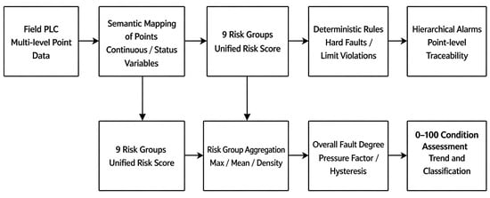
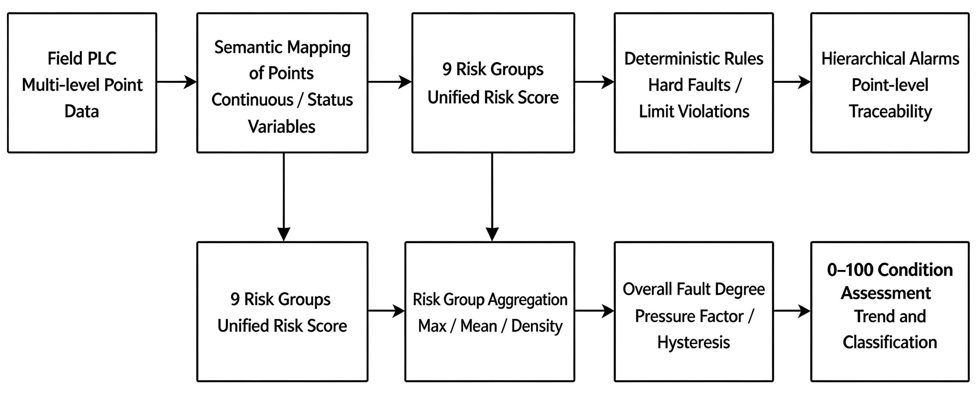
After receiving point configurations, rule parameters, and version information from the cloud, the edge node performs real-time risk modeling on the self-diagnostic data collected from the PLC. Point-risk modeling is a fundamental stage of edge-side diagnosis and includes point-semantic parsing, risk mapping of continuous and state variables, construction of risk-group features, and feature output for rule-based diagnosis and condition assessment. The detailed logic is shown in Figure 3. The nine risk-group features obtained after risk mapping are supplied to both the multi-parameter rule-base decision module and the multi-parameter fusion model. The former identifies safety-critical hard faults and ordinary threshold exceedances and provides abnormal-point traceability; the latter calculates aggregated risk-group results, the overall fault degree, and the continuous condition assessment.

Figure 3. Edge-side point-risk modeling and diagnostic-assessment logic.

Risk groups are assessment units rather than physical isolation boundaries. Point-level outputs retain the original measuring-point identifiers, timestamps, and group membership, so simultaneous or sequential anomalies involving multiple groups can be reconstructed for root-cause and propagation analysis [20]. The present rule layer does not assert unverified causal relationships; it preserves traceable evidence for subsequent system-level diagnosis.

3.2. Continuous-Variable Risk Mapping and State-Variable Binarization

The risk level of continuous variable points is not determined by their absolute values, but by the deviation degree of values relative to the safe operation interval of equipment. Five threshold parameters are maintained for each continuous variable point $\mathrm{j}\in \mathrm{C}$: lower range limit ${\mathrm{L}}_{\mathrm{j}}$, normal upper bound ${\mathrm{N}}_{\mathrm{j}}$, early warning reference value ${\mathrm{W}}_{\mathrm{j}}$, fault threshold ${\mathrm{F}}_{\mathrm{j}}$ and physical upper bound ${\mathrm{U}}_{\mathrm{j}}$.

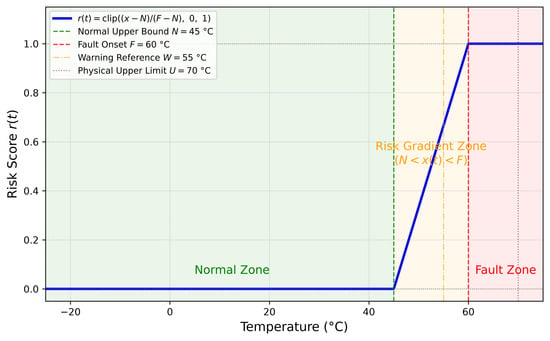
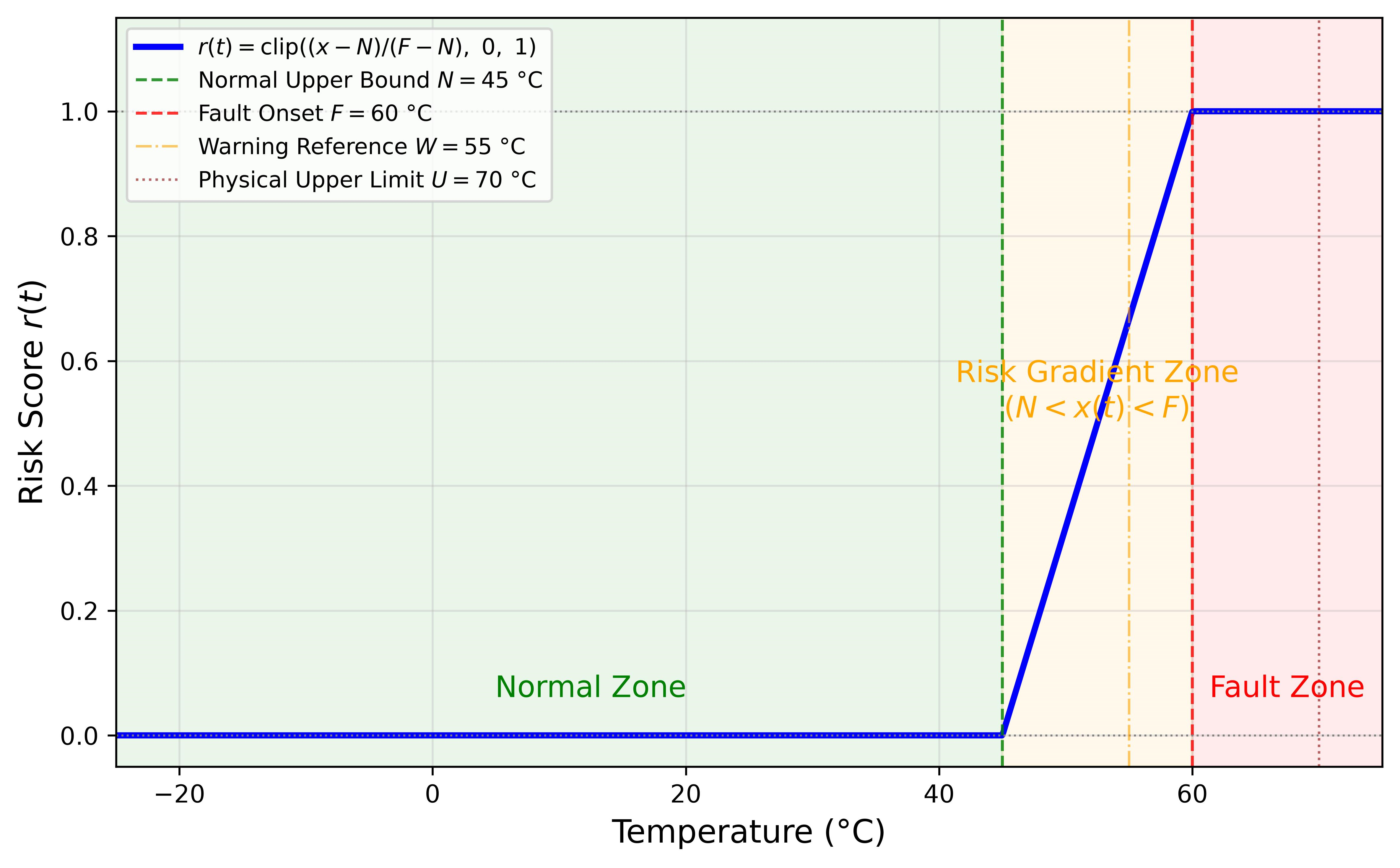
This paper adopts an upper-side risk model for all continuous variables, only detecting anomalies of excessive parameters without discussing lower limit crossing, because engineering risks of monitoring variables such as temperature, PLC load and memory utilization rate are concentrated on upper-side deviation. Taking the PLC65 temperature point (PLCD13) as an example: ${\mathrm{L}}_{\mathrm{j}}=-20$ °C, ${\mathrm{N}}_{\mathrm{j}}=45$ °C, ${\mathrm{W}}_{\mathrm{j}}=55$ °C, ${\mathrm{F}}_{\mathrm{j}}=60$ °C, ${\mathrm{U}}_{\mathrm{j}}=70$ °C.

To eliminate model bias caused by different dimensions, segmented linear risk mapping from normal upper bound ${\mathrm{N}}_{\mathrm{j}}$ to fault threshold ${\mathrm{F}}_{\mathrm{j}}$ is adopted for continuous variables, converting raw value ${\mathrm{x}}_{\mathrm{j}}\left(\mathrm{t}\right)$ into dimensionless risk score ${\mathrm{r}}_{\mathrm{j}}\left(\mathrm{t}\right)\in \left[0, 1\right]$:

$${\mathrm{r}}_{\mathrm{j}}\left(\mathrm{t}\right)=\mathrm{c}\mathrm{l}\mathrm{i}\mathrm{p}\left({\displaystyle \frac{{\mathrm{x}}_{\mathrm{j}}\left(\mathrm{t}\right)-{\mathrm{N}}_{\mathrm{j}}}{{\mathrm{F}}_{\mathrm{j}}-{\mathrm{N}}_{\mathrm{j}}}}, 0, 1\right),\mathrm{j}\in \mathrm{C}$$

(6)

The clip function is an amplitude limiter constraining the output range, with segmented semantics as follows:

When ${\mathrm{x}}_{\mathrm{j}}\left(\mathrm{t}\right)\le {\mathrm{N}}_{\mathrm{j}}$ (normal interval): ${\mathrm{r}}_{\mathrm{j}}\left(\mathrm{t}\right)=0$;

When ${\mathrm{x}}_{\mathrm{j}}\left(\mathrm{t}\right)\ge {\mathrm{F}}_{\mathrm{j}}$ (reach or exceed fault threshold): ${\mathrm{r}}_{\mathrm{j}}\left(\mathrm{t}\right)=1$;

When ${\mathrm{N}}_{\mathrm{j}}<{\mathrm{x}}_{\mathrm{j}}\left(\mathrm{t}\right)<{\mathrm{F}}_{\mathrm{j}}$ (early warning interval): risk score increases linearly from 0 to 1.

Equation (6) uses ${\mathrm{r}}_{\mathrm{j}}\left(\mathrm{t}\right)=0$ for ${\mathrm{x}}_{\mathrm{j}}\left(\mathrm{t}\right)\le {\mathrm{N}}_{\mathrm{j}}$ a linear increase for ${\mathrm{N}}_{\mathrm{j}}$ < ${\mathrm{x}}_{\mathrm{j}}\left(\mathrm{t}\right)$ < ${\mathrm{F}}_{\mathrm{j}}$, and ${\mathrm{r}}_{\mathrm{j}}\left(\mathrm{t}\right)=1$ for ${\mathrm{x}}_{\mathrm{j}}\left(\mathrm{t}\right)\ge {\mathrm{F}}_{\mathrm{j}}$. ${\mathrm{W}}_{\mathrm{j}}$ is retained as an alarm-interpretation and configuration reference, but it intentionally does not enter Equation (6); the risk score is mapped between ${\mathrm{N}}_{\mathrm{j}}$ and ${\mathrm{F}}_{\mathrm{j}}$ to maintain a monotonic transition from normal operation to the fault onset.

A risk value of 1.0 indicates that the parameter has crossed the manufacturer-defined fault-onset threshold and therefore directly participates in the rule-layer exceedance decision. Figure 4 illustrates the linear risk-mapping curve for PLC65 temperature point PLCD13.

Figure 4. Linear risk-mapping function for a continuous variable (PLC65 temperature point PLCD13).

3.3. State-Variable Binarization and Risk-Group Aggregation

Binary risk mapping is adopted for state variables. It should be noted that “1” of all status bits does not carry equivalent safety implications. This paper introduces a point semantic mapping function ${\mathrm{M}}_{\mathrm{j}}$ to distinguish fault implications of different state variables:

$${\mathrm{r}}_{\mathrm{j}}\left(\mathrm{t}\right)={\mathrm{M}}_{\mathrm{j}}\left({\mathrm{x}}_{\mathrm{j}}\left(\mathrm{t}\right)\right), \mathrm{j}\in \mathrm{S}$$

(7)

For the current dataset, all state variables have been preprocessed into binary encoding of “0 = normal, 1 = abnormal”, i.e., ${\mathrm{M}}_{\mathrm{j}}$ degenerates into an indicator function form:

$${\mathrm{r}}_{\mathrm{j}}\left(\mathrm{t}\right)=\mathbb{I}\left[{\mathrm{x}}_{\mathrm{j}}\left(\mathrm{t}\right)=1\right]$$

(8)

If the encoding rule of on-site equipment is reversed (1 = normal, 0 = fault) or there are multiple enumerated operating states, only the internal logic of ${\mathrm{M}}_{\mathrm{j}}$ needs to be adjusted, and the method possesses universal engineering adaptability.

After calculating the risk of single measuring points, three types of statistical indicators are aggregated for the same risk group g to realize dimensionality reduction of multi-point information, providing inputs for subsequent weighted fusion:

Intra-group abnormal point count ${\mathrm{A}}_{\mathrm{g}}\left(\mathrm{t}\right)$ (count of points with risk value $> {\mathsf{\theta }}_{\mathrm{r}}$, where ${\mathsf{\theta }}_{\mathrm{r}}=0.1$ is the anomaly judgment threshold to eliminate tiny fluctuations of continuous variables near the normal upper bound), intra-group maximum risk value ${\mathrm{m}\mathrm{a}\mathrm{x}}_{\mathrm{j}\in {\mathrm{I}}_{\mathrm{g}}}{\mathrm{r}}_{\mathrm{j}}\left(\mathrm{t}\right)$, intra-group average risk value ${\displaystyle \frac{1}{\left|{\mathrm{I}}_{\mathrm{g}}\right|}}{\sum }_{\mathrm{j}\in {\mathrm{I}}_{\mathrm{g}}}{\mathrm{r}}_{\mathrm{j}}\left(\mathrm{t}\right)$. Group-level summaries aggregate risk information of multiple similar measuring points into a single characterization, reducing the dimension of subsequent processing.

4. Edge-Side Adaptive Diagnosis and Early Warning Driven by a Multi-Parameter Rule Base

4.1. Hierarchical Decision Making: Hard Faults and Threshold Exceedances

4.1.1. Definition of the Safety-Critical Point Set

Hard fault trigger conditions are based on the safety-critical attribute of measuring points rather than risk group labels. Verified via on-site point tables, measuring points within the communication group (bus status, communication link fault) and power group (power supply alarm, power supply abnormality) are all fault flag signals of equipment firmware—once these status bits are set to 1, it indicates severe abnormalities of equipment communication or power supply confirmed by self-diagnosis, which should trigger immediate hard alarms. Although the fault_status group (general/serious faults of PLC modules) has a high safety weight (${\mathsf{\omega }}_{\mathrm{g}}=2.5$), some of its measuring points may correspond to non-emergency diagnostic prompts and thus are not included in hard fault trigger conditions.

Let ${\mathrm{c}}_{\mathrm{j}}\in \{0, 1\}$ be the safety-critical marker of point j, then the safety-critical point set is

$${\mathrm{S}}_{\mathrm{critical}}=\{\mathrm{j}\in \mathrm{S}\mid {\mathrm{c}}_{\mathrm{j}}=1\}$$

(9)

4.1.2. Hard Fault Judgment Rule

Hard fault ${\mathrm{y}}_{\mathrm{hard}}\left(\mathrm{t}\right)$ is triggered when any of the following conditions is satisfied:

• Safety-critical points (state variables in communication or power groups) are set to 1;
• Any continuous variable reaches its physical upper bound ${\mathrm{U}}_{\mathrm{j}}$.

Hard faults imply risks of permanent hardware damage or failure of core communication/power supply, and the system should complete rule judgment and output alarms within a single sampling period:

$${\mathrm{y}}_{\mathrm{hard}}\left(\mathrm{t}\right)=\mathbb{I}\left[\underset{\mathrm{j}\in {\mathrm{S}}_{\mathrm{critical}}}{\mathrm{m}\mathrm{a}\mathrm{x}}{\mathrm{r}}_{\mathrm{j}}\left(\mathrm{t}\right)=1\hspace{0.25em}\vee \hspace{0.25em}\underset{\mathrm{j}\in \mathrm{C}}{\mathrm{m}\mathrm{a}\mathrm{x}}\mathbb{I}\left[{\mathrm{x}}_{\mathrm{j}}\left(\mathrm{t}\right)\ge {\mathrm{U}}_{\mathrm{j}}\right]=1\right]$$

(10)

When a hard fault occurs, the system needs to output an emergency alarm immediately and activate the condition assessment latch hysteresis mechanism.

4.1.3. Threshold Out-of-Limit Judgment Rule

Threshold out-of-limit ${\mathrm{y}}_{\mathrm{limit}}\left(\mathrm{t}\right)$ is a secondary early warning anomaly, which only takes effect when no hard fault is triggered. Trigger conditions: continuous variables reach or exceed the fault threshold ${\mathrm{F}}_{\mathrm{j}}$, or non-safety-critical status bits are set to 1:

$${\mathrm{y}}_{\mathrm{limit}}\left(\mathrm{t}\right)=\mathbb{I}\left[\underset{\mathrm{j}\in \mathrm{C}}{\mathrm{m}\mathrm{a}\mathrm{x}}{\mathrm{r}}_{\mathrm{j}}\left(\mathrm{t}\right)=1\hspace{0.25em}\vee \hspace{0.25em}\underset{\mathrm{j}\in \mathrm{S}\backslash {\mathrm{S}}_{\mathrm{critical}}}{\mathrm{m}\mathrm{a}\mathrm{x}}{\mathrm{r}}_{\mathrm{j}}\left(\mathrm{t}\right)=1\right]\wedge \neg {\mathrm{y}}_{\mathrm{hard}}\left(\mathrm{t}\right)$$

(11)

The rule layer synchronously outputs the index set of all abnormal measuring points to realize accurate fault localization:

$$\mathrm{R}\left(\mathrm{t}\right)=\{\mathrm{j}\mid {\mathrm{r}}_{\mathrm{j}}\left(\mathrm{t}\right)=1\}$$

(12)

This provides maintenance personnel with traceability information accurate to the point level. When multiple points are abnormal simultaneously, the primary anomaly type is determined according to a safety priority hierarchy, in descending order: communication fault, power supply fault, system status fault, temperature exceedance, PLC load exceedance, and memory exceedance.

The design logic of the above hierarchical judgment is as follows:

• Safety-critical status bits directly come from self-diagnosis conclusions of equipment firmware, and their setting indicates internally confirmed abnormalities of equipment, which should be judged within a single sampling period;
• Continuous variables crossing ${\mathrm{F}}_{\mathrm{j}}$ are important abnormal signals, yet single-point transient out-of-limit events (accounting for 93.3%) may correspond to short-term working condition fluctuations or sensor noise, which should output early warnings instead of highest-priority hard alarms;
• Continuous variables reaching the physical upper bound ${\mathrm{U}}_{\mathrm{j}}$ are upgraded to hard faults—equipment parameters have touched physical limits, and continuous operation may lead to permanent damage.

To distinguish firmware-confirmed hard faults from raw single-frame chatter, the implementation supports a configurable persistence count ${\mathrm{p}}_{\mathrm{h}}$. A raw hard-fault indicator is promoted to ${\mathrm{y}}_{\mathrm{hard}}\left(\mathrm{t}\right)$ only after ${\mathrm{p}}_{\mathrm{h}}$ consecutive samples. In this study ${\mathrm{p}}_{\mathrm{h}}=1$ because each record is a one-minute aggregated, firmware-confirmed self-diagnosis value rather than a raw communication frame; deployments with access to sub-second raw bits can set ${\mathrm{p}}_{\mathrm{h}}>1$ without changing the remaining algorithm. Recovery is governed separately by the confirmation period $\mathrm{q}=\mathrm{3}$.

4.2. Multi-Parameter Weighted Fusion for Early Warning and Evaluation

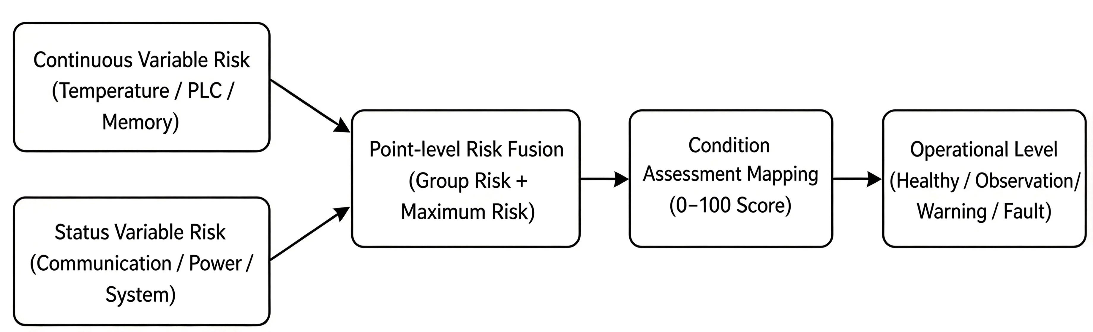
The goal of condition assessment is to compress multi-point, multi-type and multi-time-scale operation states into a continuous index ranging from 0 to 100, enabling maintenance personnel to intuitively observe the relative risk evolution of equipment from healthy, observation, early warning to fault. Different from single-point alarms, condition assessment should reflect the overall operation pressure of equipment, being sensitive to hard faults while avoiding drastic jumps caused by single slight fluctuations. The multi-parameter fusion structure used for condition assessment is shown in Figure 5.

Figure 5. Multi-parameter fusion structure for early-warning assessment.

Figure 5. Multi-parameter fusion structure for early-warning assessment.

4.2.1. Point-Risk and Risk-Group Modeling

Device points are divided into G risk groups including temperature group, PLC load group, memory group, communication group, power supply group, program operation group and system status group. Each risk group g contains several measuring points ${\mathrm{I}}_{\mathrm{g}}$. The risk group score is jointly determined by intra-group maximum risk, average risk and anomaly density.

$${\mathrm{R}}_{\mathrm{g}}\left(\mathrm{t}\right)={\mathsf{\alpha }}_{\mathrm{g}}\underset{\mathrm{j}\in {\mathrm{I}}_{\mathrm{g}}}{\max }{\mathrm{r}}_{\mathrm{j}}\left(\mathrm{t}\right)+{\mathsf{\beta }}_{\mathrm{g}}\left({\displaystyle \frac{1}{\left|{\mathrm{I}}_{\mathrm{g}}\right|}}\right){\mathsf{\Sigma }}_{\mathrm{j}\in {\mathrm{I}}_{\mathrm{g}}}{\mathrm{r}}_{\mathrm{j}}\left(\mathrm{t}\right)+{\displaystyle \frac{{\mathsf{\eta }}_{\mathrm{g}}{\mathrm{A}}_{\mathrm{g}}\left(\mathrm{t}\right)}{\left|{\mathrm{I}}_{\mathrm{g}}\right|}}$$

(13)

where ${\mathrm{A}}_{\mathrm{g}}\left(\mathrm{t}\right)$ denotes the number of anomaly points within the risk group; ${\mathsf{\alpha }}_{\mathrm{g}}, {\mathsf{\beta }}_{\mathrm{g}}, \mathrm{a}\mathrm{n}\mathrm{d}{ \mathsf{\eta }}_{\mathrm{g}}$ are weights that can be configured according to business importance and satisfy ${\mathsf{\alpha }}_{\mathrm{g}}+{\mathsf{\beta }}_{\mathrm{g}}+{\mathsf{\eta }}_{\mathrm{g}}=$1. For critical risk groups such as power supply, communication, and severity faults, the maximum risk weight should be set higher to prioritize the detection of single-point severe anomalies; for the continuous-point group, the three weights are configured in a balanced manner. The complete parameter configuration for each group is presented in Table 4.

Table 4. Risk-group weights and score coefficients.

Risk Group	${\mathsf{\omega }}_{\mathbf{g}}$	${\mathsf{\alpha }}_{\mathbf{g}}$	${\mathsf{\beta }}_{\mathbf{g}}$	${\mathsf{\eta }}_{\mathbf{g}}$	Design Rationale
Communication	3.0	0.7	0.2	0.1	Safety-critical group; triggers a hard fault
Power	3.0	0.7	0.2	0.1	Safety-critical group; triggers a hard fault
Fault_status	2.5	0.6	0.3	0.1	High-weight group (does not directly trigger a hard fault)
Temperature	1.5	0.5	0.4	0.1	Continuous-variable group
PLC_load	1.5	0.5	0.4	0.1	Continuous-variable group
Memory	1.5	0.5	0.4	0.1	Continuous-variable group
System_status	1.0	0.5	0.4	0.1	General state group
Program	1.0	0.5	0.4	0.1	General state group
Temperature_alarm	1.0	0.5	0.4	0.1	General state group

4.2.2. Comprehensive Fault Degree and Condition Assessment Mapping

Weighted normalized average risk based on group safety weights:

$$\stackrel{\mathrm{‾}}{\mathrm{R}}\left(\mathrm{t}\right)={\displaystyle \frac{{\displaystyle {\sum }_{\mathrm{g}=1}^{\mathrm{G}}}{\mathsf{\omega }}_{\mathrm{g}}{\mathrm{R}}_{\mathrm{g}}\left(\mathrm{t}\right)}{{\displaystyle {\sum }_{\mathrm{g}=1}^{\mathrm{G}}}{\mathsf{\omega }}_{\mathrm{g}}}}$$

(14)

Fuse global single-point extreme risk to avoid dilution of single-point severe anomalies by intra-group averaging:

$$\mathrm{D}\left(\mathrm{t}\right)=100\cdot \mathrm{clip}\left(\left(1-\mathsf{\rho }\right)\cdot \stackrel{\mathrm{‾}}{\mathrm{R}}\left(\mathrm{t}\right)+\mathsf{\rho }\cdot \underset{\mathrm{j}}{\mathrm{m}\mathrm{a}\mathrm{x}}{\mathrm{r}}_{\mathrm{j}}\left(\mathrm{t}\right),\hspace{0.25em}0,\hspace{0.25em}1\right)$$

(15)

where ${\mathsf{\omega }}_{\mathrm{g}}$ denotes the fusion weight of risk group g, with $\sum {\mathsf{\omega }}_{\mathrm{g}}=16.0$; $\mathsf{\rho }=0.15$ is the global maximum risk proportion coefficient, indicating explicitly that the global maximum risk accounts for 15% of the composite fault degree, thereby ensuring that an extreme risk value at any single point can independently influence the device fault degree without being diluted by intra-group averaging.

4.2.3. Condition Assessment Mapping and Time-Series Optimization Mechanism

Map fault degree to condition assessment and impose hard fault mandatory constraints:

$${\mathrm{H}}_{\mathrm{raw}}\left(\mathrm{t}\right)=100-\mathrm{D}\left(\mathrm{t}\right)-\mathsf{\kappa }\cdot \mathrm{P}\left(\mathrm{t}\right)\cdot \mathbb{I}\left[\mathrm{D}\left(\mathrm{t}\right)<{\mathrm{D}}_{\mathrm{warn}}\right]$$

(16)

$${\mathrm{H}}_{\mathrm{raw}}\left(\mathrm{t}\right)=\mathrm{m}\mathrm{i}\mathrm{n}\left({\mathrm{H}}_{\mathrm{raw}}\left(\mathrm{t}\right),{\mathrm{H}}_{\mathrm{fault}}^{\mathrm{m}\mathrm{a}\mathrm{x}}\right), \mathrm{if} {\mathrm{y}}_{\mathrm{hard}}\left(\mathrm{t}\right)=1$$

(17)

where $\mathsf{\kappa }=3.0$ is the stress coefficient, ${\mathrm{D}}_{\mathrm{warn}}=15.0$ is the activation threshold for the stress term, and ${\mathrm{H}}_{\mathrm{fault}}^{\mathrm{m}\mathrm{a}\mathrm{x}}=25$ is the upper bound of the hard fault condition assessment. The normal operating stress $\mathrm{P}\left(\mathrm{t}\right)$ is determined by the relative position of the continuous points within the normal range:

$$\mathrm{P}\left(\mathrm{t}\right)={\displaystyle \frac{1}{\left|\mathrm{C}\right|}}\sum _{\mathrm{j}\in \mathrm{C}}\mathrm{clip}\left({\displaystyle \frac{{\mathrm{x}}_{\mathrm{j}}\left(\mathrm{t}\right)-{\mathrm{L}}_{\mathrm{j}}}{{\mathrm{N}}_{\mathrm{j}}-{\mathrm{L}}_{\mathrm{j}}}},\hspace{0.25em}0,\hspace{0.25em}1\right)$$

(18)

The physical implication of $\mathrm{P}\left(\mathrm{t}\right)$ is “where the equipment currently operates within the normal interval”—$\mathrm{P}\left(\mathrm{t}\right)\approx 0$ means parameters are close to the lower bound of the normal interval (equipment operates under light load), while $\mathrm{P}\left(\mathrm{t}\right)\approx 1$ means parameters are close to the upper bound of the normal interval (equipment operates under heavy load). The pressure term only takes effect when the equipment is overall healthy ($\mathrm{D}\left(\mathrm{t}\right)<{\mathrm{D}}_{\mathrm{warn}}$), enabling subtle differentiation of about three points between low-load and high-load operation under fully normal conditions.

The condition assessment defined in this paper is a relative comprehensive evaluation indicator constructed based on equipment point risks and engineering weights, used for state tracking and risk sorting of the same equipment. Its value is not externally calibrated with maintenance records, equipment remaining life or expert scores, and does not directly equal equipment remaining life or real failure probability. The index is therefore evaluated only for internal temporal consistency and association with rule-defined fault events; it is not interpreted as an externally validated degradation, remaining-useful-life, or failure-probability score.

Instantaneous noise and communication jitter exist in industrial sites. Exponential smoothing is adopted for time-domain filtering in non-hard fault scenarios; for hard faults, condition assessment jumps directly to the fault interval without smoothing. To realize recovery hysteresis—ensuring that equipment cannot be marked “healthy” immediately after a single normal sampling—a hard fault latch state variable ${\mathrm{z}}_{\mathrm{hard}}\left(\mathrm{t}\right)$ is introduced:

$${\mathrm{z}}_{\mathrm{hard}}\left(\mathrm{t}\right)=\left\{\begin{array}{ll}1,& {\mathrm{y}}_{\mathrm{hard}}\left(\mathrm{t}\right)=1\\ 0,& {\mathrm{z}}_{\mathrm{hard}}\left(\mathrm{t}-1\right)=1 \mathrm{a}\mathrm{n}\mathrm{d} {\mathrm{y}}_{\mathrm{hard}}=0 \mathrm{for}\mathrm{q}\mathrm{consecutive}\mathrm{sampling}\mathrm{periods}\hspace{0.25em}\\ {\mathrm{z}}_{\mathrm{hard}}\left(\mathrm{t}-1\right),& \mathrm{o}\mathrm{t}\mathrm{h}\mathrm{e}\mathrm{r}\mathrm{w}\mathrm{i}\mathrm{s}\mathrm{e}\end{array}\right.$$

(19)

Under the latch state, condition assessment is mandatorily constrained within the upper limit of the fault interval ${\mathrm{H}}_{\mathrm{fault}}^{\mathrm{m}\mathrm{a}\mathrm{x}}$:

$${\mathrm{H}}_{\mathrm{c}}\left(\mathrm{t}\right)=\left\{\begin{array}{ll}\mathrm{m}\mathrm{i}\mathrm{n}\left({\mathrm{H}}_{\mathrm{raw}}\left(\mathrm{t}\right),\hspace{0.25em}{\mathrm{H}}_{\mathrm{fault}}^{\mathrm{m}\mathrm{a}\mathrm{x}}\right),& {\mathrm{z}}_{\mathrm{hard}}\left(\mathrm{t}\right)=1\\ {\mathrm{H}}_{\mathrm{raw}}\left(\mathrm{t}\right),& {\mathrm{z}}_{\mathrm{hard}}\left(\mathrm{t}\right)=0\end{array}\right.$$

(20)

Finally, exponential smoothing is applied to non-latch states, while latch states retain original values:

$$\tilde{\mathrm{H}}\left(\mathrm{t}\right)=\left\{\begin{array}{ll}{\mathrm{H}}_{\mathrm{c}}\left(\mathrm{t}\right),& {\mathrm{z}}_{\mathrm{hard}}\left(\mathrm{t}\right)=1\\ \mathsf{\lambda }{\mathrm{H}}_{\mathrm{c}}\left(\mathrm{t}\right)+\left(1-\mathsf{\lambda }\right)\tilde{\mathrm{H}}\left(\mathrm{t}-1\right),& {\mathrm{z}}_{\mathrm{hard}}\left(\mathrm{t}\right)=0\end{array}\right.$$

(21)

where $\mathsf{\lambda }=0.5$ is the exponential smoothing coefficient, $\mathrm{q}=3$ is the number of recovery confirmation periods, and ${\mathrm{H}}_{\mathrm{fault}}^{\mathrm{m}\mathrm{a}\mathrm{x}}=25$ is the upper bound of the hard fault condition assessment. This mechanism ensures that when a hard fault is triggered, the condition assessment immediately enters the fault interval $\left[0, 25\right]$; after the hard fault signal disappears, the condition assessment continues to remain in the fault interval until normal status is confirmed for three consecutive sampling periods; thereafter, it gradually recovers under exponential smoothing, thereby avoiding transient jumps.

Condition assessment is divided into five grades as shown in Table 5. Note that grade boundaries adopt left-closed and right-open definition to eliminate boundary overlap.

Table 5. Condition assessment grades and operation and maintenance suggestions.

Condition Assessment Interval	Condition Grade	Engineering Implication	Recommended Actions
[90, 100]	Healthy	Stable operation without obvious risks	Routine monitoring
[75, 90)	Observation	Slight pressure or weak risks exist	Focus on trends, increase inspection frequency
[60, 75)	Early warning	Continuous abnormal trends or anomalies of multiple risk groups exist	Arrange inspections, prepare spare parts or remote confirmation
[30, 60)	High risk	Local faults or anomalies of multiple risk groups	On-site troubleshooting, generate work orders
[0, 30)	Fault	Confirmed faults or hard rules triggered	Immediate disposal, linkage shutdown protection if necessary

Rule hierarchical judgment and condition assessment share the same standardized risk feature space, forming a collaborative operation logic of “discrete abnormal event triggering + continuous state characterization for a long time”: the rule layer accurately captures discrete abnormal events such as hard faults and ordinary out-of-limit events, providing time anchors of fault triggering for the condition assessment time-series curve, and constrains the rise rate of the condition assessment after fault removal relying on the recovery hysteresis mechanism; condition assessment continuously characterizes the operation margin and load pressure of equipment during fault-free periods with continuous quantitative scores. The two modules output hierarchical alarm information and refined condition assessment in parallel, constructing a dual-channel monitoring support system oriented to operation and maintenance.

5. Experimental Validation

5.1. Experimental Setup

The experimental objects are five production-control equipment units at oil and gas stations, with equipment information shown in Table 6. The data collection period is 1 min, covering a time span of seven days, with 10,080 records per equipment and a total of 50,400 records. The 5 equipment units contain 80 self-diagnosis measuring points in total (71 state variables, 9 continuous variables), covering all 9 risk groups. The five-level threshold configuration of continuous variables for each piece of equipment is shown in Table 7.

Table 6. Experimental device configuration.

Device ID	Type	Total Measuring Points	Continuous Variables	State Variables
PLC65	PLC	25	3	22
PLC64	PLC	14	1	13
PLC34	PLC	11	3	8
PLC013	PLC	15	1	14
PLC3Z	PLC	15	1	14

Table 7. Continuous-variable threshold configuration.

Device	Measuring Point	Unit	Normal Range	Warning Upper Limit (Wj)	Fault Onset (Fj)	Physical Upper Limit (Uj)
PLC65	PLCD13 (temperature)	°C	[−20, 45]	55	60	70
PLC65	PLCD14 (memory)	%	[0, 75]	85	90	100
PLC65	PLCD16 (PLC load)	%	[0, 70]	85	90	100
PLC64	PLCC5 (temperature)	°C	[−20, 45]	55	60	70
PLC34	PLCB1 (PLC load)	%	[0, 70]	85	90	100
PLC34	PLCB2 (temperature A)	°C	[0, 50]	60	65	75
PLC34	PLCB3 (temperature B)	°C	[0, 50]	60	65	75
PLC013	PLCA5 (PLC load)	%	[0, 70]	85	90	100
PLC3Z	PLCA5 (PLC load)	%	[0, 70]	85	90	100

5.2. Rule-Layer Fault Detection

The proposed rule layer was applied to detect continuous-variable threshold-exceedance events for PLC65. Table 8 summarizes the distribution of fault types.

Table 8. Distribution of threshold out-of-limit event types of PLC65 (7 days).

Fault Type	Sampling Points	Proportion (%)
Temperature out-of-limit	156	1.55
Memory out-of-limit	153	1.52
PLC load out-of-limit	137	1.36
Temperature + Memory joint out-of-limit	92	0.91
Temperature + PLC load joint out-of-limit	82	0.81
Memory + PLC load joint out-of-limit	79	0.78
Three-variable joint out-of-limit	22	0.22
Total	721	7.15

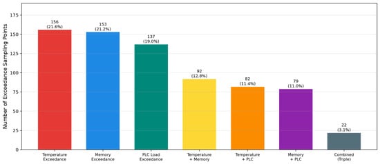
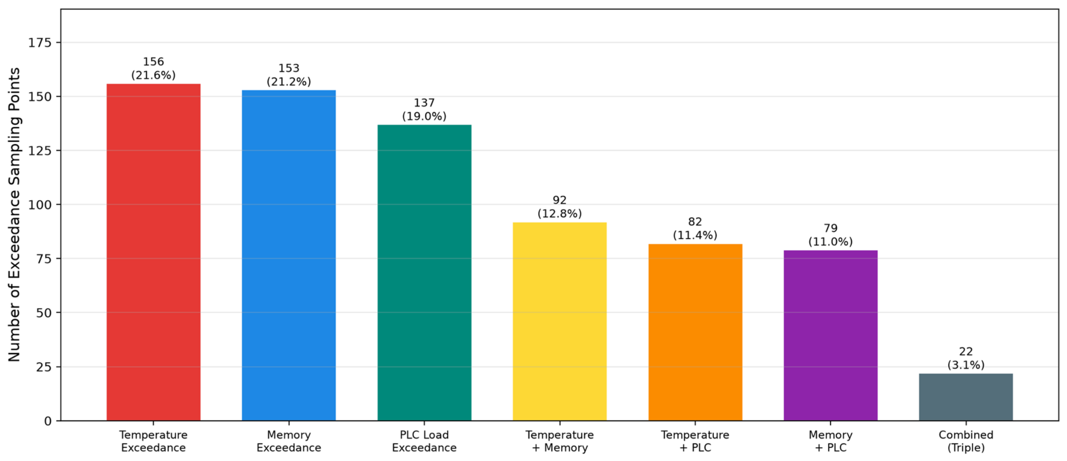
PLC65 has a total of 721 sampling points of continuous variable threshold out-of-limit within 7 days, accounting for 7.15% of total sampling points. Among these, single-variable exceedances predominated (446 points, 61.9%), followed by two-variable concurrent exceedances (253 points, 35.1%), with three-variable simultaneous exceedances being the least frequent (22 points, 3.0%). Figure 6 is a bar chart showing the distribution of each out-of-limit type and combined out-of-limit combinations.

Figure 6. Distribution of Fault Types of PLC65.

For the 22 state-variable points of PLC65, the anomaly-triggering statistics over seven days are listed in Table 9.

Table 9. State-variable anomaly statistics of PLC65.

Statistical Indicator	Value
Total state measuring points	22
Total observation records	221,760
Total anomaly times	1495
Overall anomaly rate	0.67%
Single-variable anomaly rate range	0.5–0.9%

5.3. Temporal Overlap Analysis

The triggering frequencies of state-variable anomalies (0.67%) and continuous-variable exceedances (7.15%) differed by approximately one order of magnitude. To quantify their temporal association, the Jaccard overlap was calculated as follows:

$$\mathrm{J}={\displaystyle \frac{{\sum }_{\mathrm{t}}\mathbb{I}\left[{\mathrm{y}}_{\mathrm{S}}\left(\mathrm{t}\right)=1\wedge {\mathrm{y}}_{\mathrm{C}}\left(\mathrm{t}\right)=1\right]}{{\sum }_{\mathrm{t}}\mathbb{I}\left[{\mathrm{y}}_{\mathrm{S}}\left(\mathrm{t}\right)=1\vee {\mathrm{y}}_{\mathrm{C}}\left(\mathrm{t}\right)=1\right]}}$$

(22)

where ${\mathrm{y}}_{\mathrm{S}}\left(\mathrm{t}\right)$ indicates the presence of any status-point anomaly at time t, and ${\mathrm{y}}_{\mathrm{C}}\left(\mathrm{t}\right)$ indicates that at least one continuous point exceeds its fault onset at time t. Taking PLC65 as an example: only status-point anomalies occurred for 287 min, only continuous-point exceedances for 104 min, both triggered simultaneously for 617 min, with a union of 1008 min. The calculated Jaccard overlap is $\mathrm{J}=617/1008=0.61$, and the conditional probabilities are $\mathrm{P}\left({\mathrm{y}}_{\mathrm{S}}=1\mid {\mathrm{y}}_{\mathrm{C}}=1\right)=85.6\%$ and $\mathrm{P}\left({\mathrm{y}}_{\mathrm{C}}=1\mid {\mathrm{y}}_{\mathrm{S}}=1\right)=68.3\%$.

These results demonstrate substantial temporal overlap between state-variable anomalies and continuous-variable exceedances in the dataset. Safety-critical status points in the communication or power groups triggered hard faults for 495 min, corresponding to 4.91% of the operating time and indicating communication or power anomalies during approximately 4.9% of operation. The approximately tenfold difference in triggering frequency and the pronounced temporal overlap (Jaccard coefficient 0.61) demonstrate complementary temporal coverage rather than, by themselves, prove improved detection accuracy. Monitoring only continuous variables would miss 287 min of status-only anomalies, whereas monitoring only state variables would miss 104 min of continuous-only exceedances.

5.4. Event-Duration Analysis

The durations of 673 independent threshold-exceedance events detected for PLC65, after consecutive exceedance samples were merged, are summarized in Table 10.

Table 10. Duration distribution of PLC65 threshold-exceedance events.

Duration	Number of Events	Proportion (%)
1 min (single sample)	628	93.3
2–3 min (2–3 samples)	45	6.7
>3 min	0	0.0

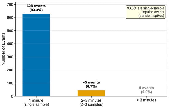
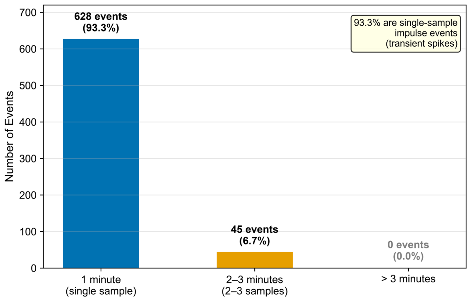
A total of 93.3% of the exceedance events manifested as single-sample pulses, where a parameter abruptly rose from its normal value to an exceedance level and returned to normal within the next sampling minute. Multi-sample events lasting 2–3 min accounted for only 6.7%, and no event lasted longer than 3 min. The advantages of the hierarchical decision strategy are evident for this transient-dominated pattern. A safety-critical status bit immediately generates a hard alarm within one sampling period, whereas an isolated continuous-variable exceedance without a safety-critical status anomaly is recorded as a warning event. The alarm level may subsequently be escalated through consecutive-sample confirmation or trend analysis, reducing alarm fatigue caused by numerous transient spikes. Figure 7 shows the event-duration distribution.

Figure 7. Distribution of PLC65 event durations.

5.5. Comparison of Fault Diagnosis Across Five Devices

The hierarchical decision procedure was applied uniformly to all five experimental devices. Their continuous-variable exceedance rates, proportions of transient events, and state-variable anomaly rates are compared in Table 11.

Table 11. Comparison of fault-diagnosis results for the five devices.

Device	Number of Continuous Variables	Exceedance Rate (%)	Total Events	Single-Sample Events (%)	Multi-Sample Events (%)	State-Variable Abnormality Rate (%)
PLC65	3	7.15	673	93.3	6.7	0.67
PLC64	1	7.08	658	91.8	8.2	1.37
PLC34	3	7.34	680	92.6	7.4	1.83
PLC013	1	7.19	677	93.6	6.4	1.28
PLC3Z	1	7.20	670	92.5	7.5	1.25

The following observations can be drawn from Table 11:

(1)

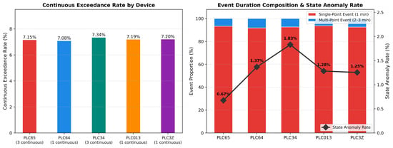
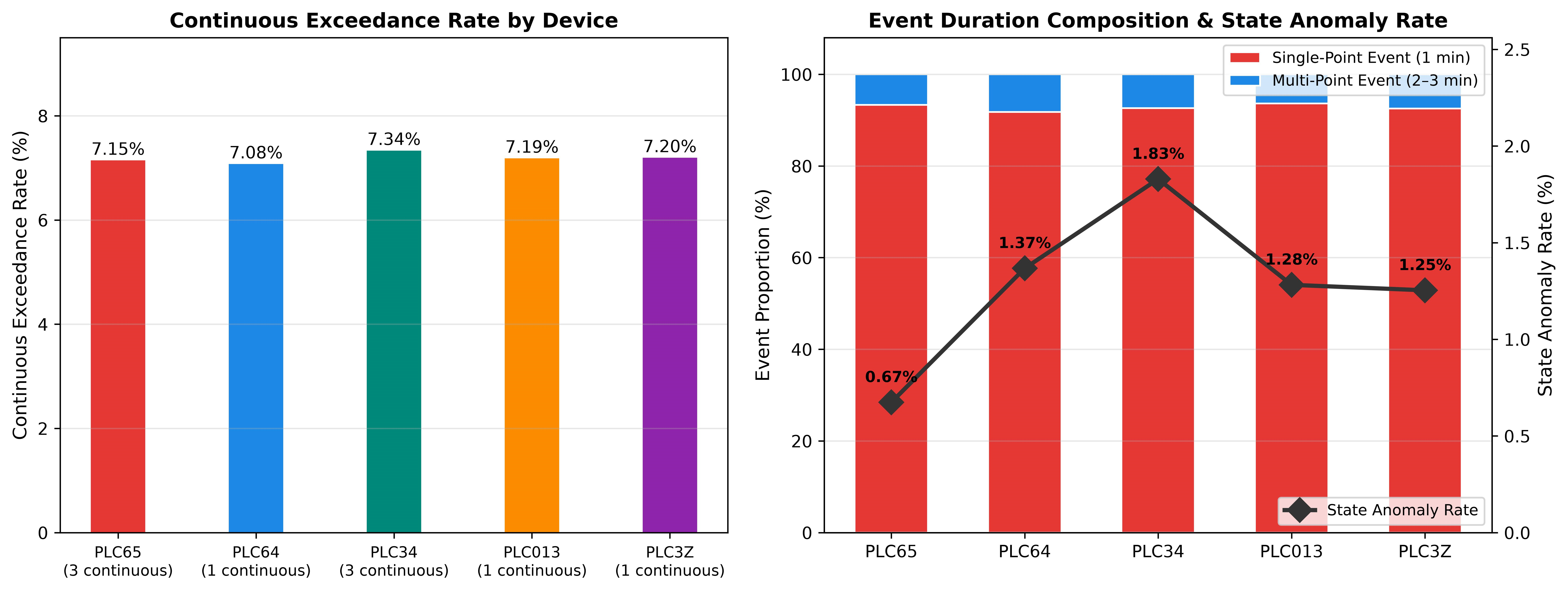
Consistency of exceedance rates. The continuous-variable exceedance rates of the five devices were highly similar (7.08–7.34%), and the proportions of single-sample events ranged from 91.8% to 93.6%, indicating consistency across the dataset. In actual industrial environments, anomaly rates may vary substantially with operating conditions and equipment age; therefore, the consistency observed here should not be directly generalized to heterogeneous equipment populations.

(2)

Differences in continuous-variable dimensionality. For the single-continuous-variable devices PLC64, PLC013, and PLC3Z, every exceedance event was triggered by one variable. The multi-continuous-variable devices PLC65 and PLC34 produced richer combinations of joint exceedances. This distinction is practically important for subsequent statistical-learning models, because anomaly-boundary identification in a multidimensional feature space requires sufficient samples of joint exceedances.

(3)

Differences between status and continuous variables. State-variable anomaly rates (0.67–1.83%) were approximately 4–10 times lower than continuous-variable exceedance rates (7.08–7.34%). The two signal types differ substantially in triggering frequency and physical meaning, indicating that their combined use improves coverage of anomalies with different physical semantics. Figure 8 compares the exceedance rates and event-duration compositions of the five devices in a two-panel format.

Figure 8. Comparison of fault-diagnosis results for the five devices ((left): exceedance rate; (right): event-duration composition).

5.6. Case Analysis of Fault Events

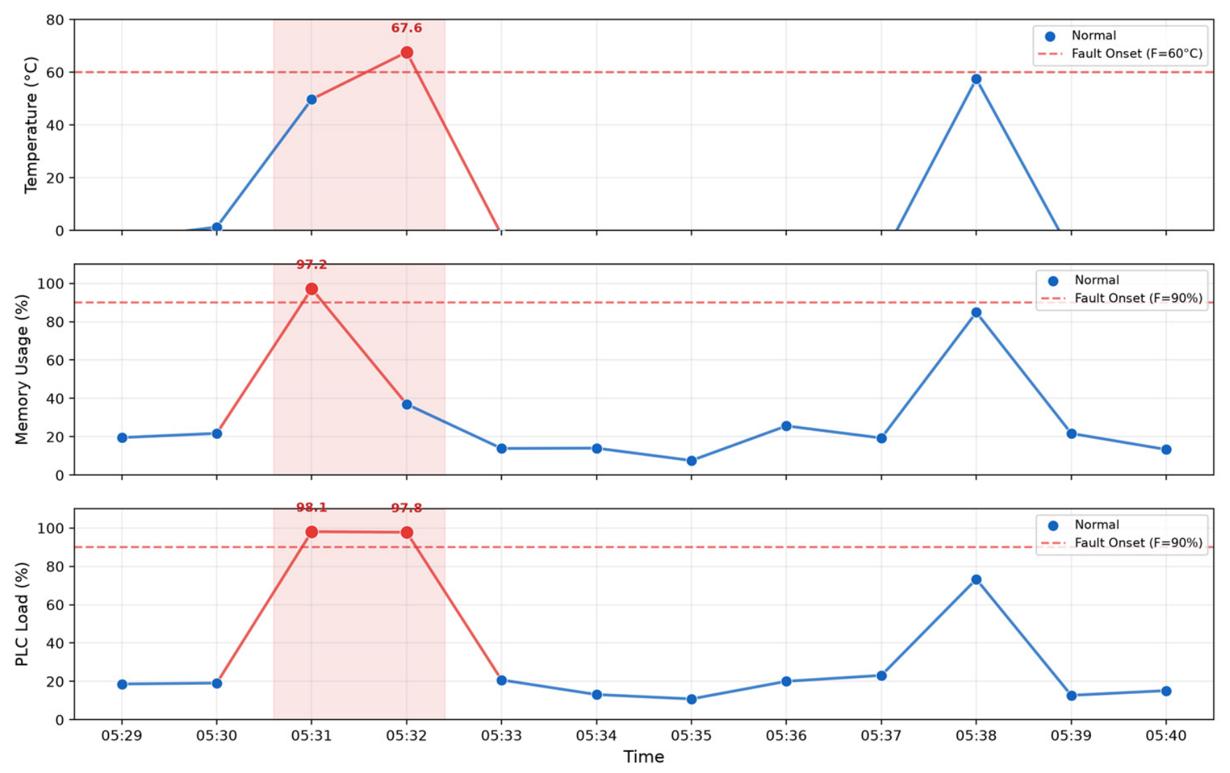
To illustrate the specific manifestation of exceedance events in time-series data, Table 12 presents a representative two-minute multivariable joint-exceedance event from PLC65.

Table 12. Example of a multi-point fault event in PLC65.

Time	Temperature (°C)	Memory (%)	PLC Load (%)	Status
05:29	−3	20	19	Normal
05:30	1	22	19	Normal
05:31	50	97	98	Fault (combined memory and PLC-load exceedance)
05:32	68	37	98	Fault (combined temperature and PLC-load exceedance)
05:33	−2	14	21	Normal
05:34	−4	14	13	Normal

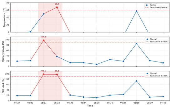
Before and after the event, all parameters remained stable within their normal ranges. Two successive two-variable exceedances occurred at 05:31 and 05:32: memory plus PLC load at 05:31 and temperature plus PLC load at 05:32. The variables returned rapidly to normal at 05:33. The entire event lasted only two minutes and did not exhibit a sustained multi-sample trend. This example confirms that short-term impact-type exceedances dominated the operating data (93.3%). In such scenarios, exponential smoothing and recovery hysteresis effectively suppress abrupt condition assessment changes caused by isolated pulse anomalies and improve the stability of maintenance visualization. Figure 9 shows the complete time-series evolution of the event.

Figure 9. Time series of a multi-point fault event for PLC65.

5.7. Multi-Parameter Fusion and Condition Assessment Time Series

The 7-day condition assessment sequence of PLC65 is calculated in this section to verify the distribution characteristics of the condition assessment formula under real on-site data, hard fault constraint effects and dynamic responses during anomaly occurrence and recovery. The complete model parameter settings are: pressure term coefficient $\mathsf{\kappa }=3.0$, smoothing coefficient $\mathsf{\lambda }=0.5$, recovery confirmation period $\mathrm{q}=3$, hard fault condition assessment upper limit ${\mathrm{H}}_{\mathrm{f}\mathrm{a}\mathrm{u}\mathrm{l}\mathrm{t}}^{\mathrm{m}\mathrm{a}\mathrm{x}}=25$. The resulting distribution of PLC65 condition grades over the seven-day period is summarized in Table 13.

Table 13. Distribution of PLC65 condition grades.

Condition Grade	Interval	Number of Records	Percentage (%)
Healthy	[90, 100]	6210	61.6
Observation	[75, 90)	1839	18.2
Warning	[60, 75)	535	5.3
High risk	[30, 60)	77	0.8
Fault	[0, 30)	1419	14.1

Table 13. Distribution of PLC65 condition grades.

Condition Grade	Interval	Number of Records	Percentage (%)
Healthy	[90, 100]	6210	61.6
Observation	[75, 90)	1839	18.2
Warning	[60, 75)	535	5.3
High risk	[30, 60)	77	0.8
Fault	[0, 30)	1419	14.1

A total of 1419 records fell within the fault interval, accounting for 14.08%. Of these, the original hard-fault condition—direct assertion of a safety-critical status bit or a continuous variable reaching its physical upper limit—occurred for 495 min, or 4.91%. Under the recovery-confirmation mechanism, the hard-fault latch remained active for 1419 min in total. Thus, the higher proportion of fault-interval records relative to the raw hard-fault duration is not duplicate counting; it is the direct result of safety confirmation applied to short-term recovery signals by the hysteresis mechanism.

For the complete model, the mean condition assessment was 82.44, the standard deviation was 25.07, the minimum was 25, and the maximum was 99.53. The healthy interval accounted for 61.61% of records, while the observation and warning intervals together accounted for 23.55%. These intermediate grades mainly corresponded to continuous variables near their upper normal limits, anomalies in non-safety-critical status points, and smoothed recovery after fault clearance. When a hard fault occurred, the condition assessment was constrained to the upper boundary of the fault interval (25) without smoothing; after the latch was released, it gradually recovered through exponential smoothing. This behavior is consistent with the safety-oriented principle of rapid fault response and cautious recovery confirmation.

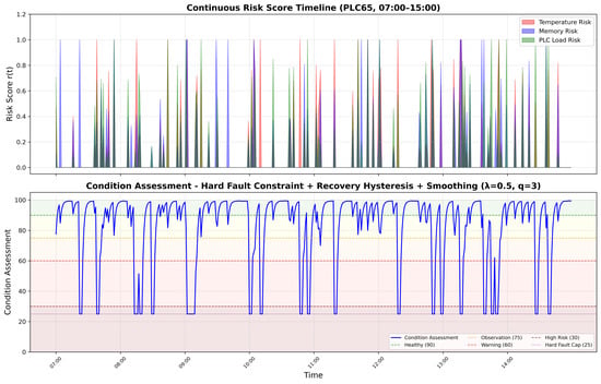
Figure 10 shows the continuous-variable risks and condition assessment over a representative period for PLC65. During normal operation, the condition assessment remained high; it decreased with continuous-variable exceedances; it entered the fault interval immediately when a safety-critical status point was asserted; and after the anomaly disappeared, it recovered gradually under the combined effects of recovery hysteresis and exponential smoothing.

Figure 10. Time series of the PLC65 condition assessment and continuous-variable risks.

5.8. Ablation Experiments and Parameter-Sensitivity Analysis

Ablation experiments were conducted on all 10,080 PLC65 records to examine the independent contributions of the condition-assessment model components. Except for the removed component, all parameters were identical to those of the complete model. Evaluation metrics included the mean and standard deviation of the condition assessment, the proportion of each condition grade, the number of condition-grade transitions, and the mean absolute change between adjacent samples. The number of grade transitions reflects how frequently the output crosses maintenance-grade boundaries, whereas the mean absolute change measures minute-scale score fluctuations. The ablation-experiment settings are summarized in Table 14. The ablation-experiment settings are summarized in Table 14. The overall metrics are summarized in Table 15, and the corresponding condition-grade proportions are reported in Table 16.

In the isolated hard-fault-constraint experiment, only the interval cap in Equation (17) was removed; hard-fault detection and the recovery-latch logic were retained. This comparison therefore isolates the contribution of the constraint rather than confounding it with recovery hysteresis.

To facilitate comparison, the condition-grade proportions of the five ablation configurations are visualized in Figure 11.

Table 14. Ablation-experiment settings.

Experimental Group	Hard-Fault Constraint	Operating-Pressure Term	Recovery Hysteresis	Exponential Smoothing
Full model	√	√	√	√
Without operating-pressure term	√	—	√	√
Without hard-fault constraint	—	√	√	√
Without recovery hysteresis	√	√	—	√
Without exponential smoothing	√	√	√	—

√ indicates that the component is enabled; — indicates that the component is removed.

Table 14. Ablation-experiment settings.

Experimental Group	Hard-Fault Constraint	Operating-Pressure Term	Recovery Hysteresis	Exponential Smoothing
Full model	√	√	√	√
Without operating-pressure term	√	—	√	√
Without hard-fault constraint	—	√	√	√
Without recovery hysteresis	√	√	—	√
Without exponential smoothing	√	√	√	—

√ indicates that the component is enabled; — indicates that the component is removed.

Table 15. Overall metrics of the PLC65 ablation experiments.

Experimental Group	Mean	Standard Deviation	Minimum	Number of Grade Transitions	Mean Absolute Change
Full model	82.44	25.07	25.00	3437	8.25
Without operating-pressure term	82.93	25.30	25.00	3412	8.34
Without hard-fault constraint	93.36	10.18	37.47	3216	6.83
Without recovery hysteresis	88.59	17.48	25.00	3799	9.09
Without exponential smoothing	85.32	26.10	25.00	3167	11.87

Table 15. Overall metrics of the PLC65 ablation experiments.

Experimental Group	Mean	Standard Deviation	Minimum	Number of Grade Transitions	Mean Absolute Change
Full model	82.44	25.07	25.00	3437	8.25
Without operating-pressure term	82.93	25.30	25.00	3412	8.34
Without hard-fault constraint	93.36	10.18	37.47	3216	6.83
Without recovery hysteresis	88.59	17.48	25.00	3799	9.09
Without exponential smoothing	85.32	26.10	25.00	3167	11.87

Table 16. Condition-grade proportions in the PLC65 ablation experiments (%).

Experimental Group	Healthy	Observation	Warning	High Risk	Fault
Full model	61.61	18.24	5.31	0.76	14.08
Without operating-pressure term	63.28	16.65	5.23	0.76	14.08
Without hard-fault constraint	78.20	15.46	3.22	3.12	0.00
Without recovery hysteresis	68.33	20.05	5.88	0.82	4.91
Without exponential smoothing	72.29	6.39	6.65	0.60	14.08

Table 16. Condition-grade proportions in the PLC65 ablation experiments (%).

Experimental Group	Healthy	Observation	Warning	High Risk	Fault
Full model	61.61	18.24	5.31	0.76	14.08
Without operating-pressure term	63.28	16.65	5.23	0.76	14.08
Without hard-fault constraint	78.20	15.46	3.22	3.12	0.00
Without recovery hysteresis	68.33	20.05	5.88	0.82	4.91
Without exponential smoothing	72.29	6.39	6.65	0.60	14.08

To facilitate comparison, the condition-grade proportions of the five ablation configurations are visualized in Figure 11.

Figure 11. Comparison of condition-grade distributions in the ablation study.

Figure 11. Comparison of condition-grade distributions in the ablation study.

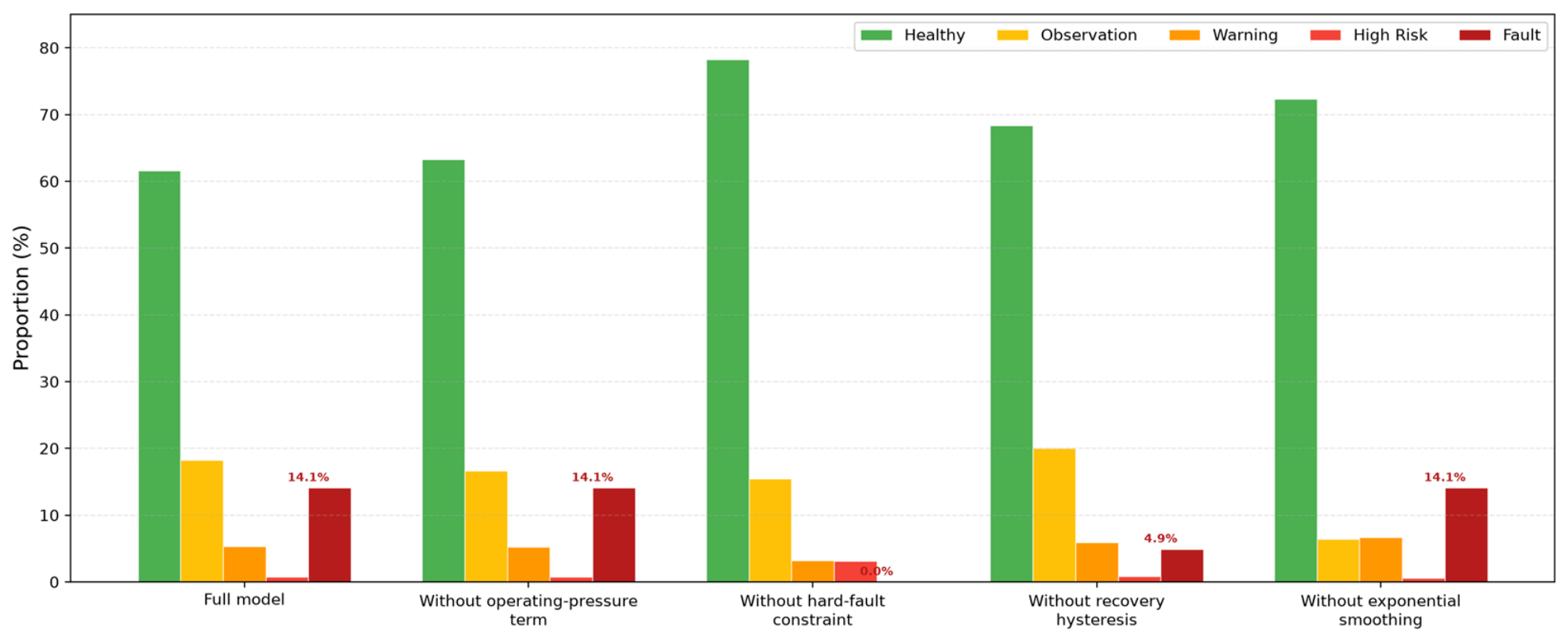
• Effect of the stress term. Eliminating the operating-stress term raises the average condition assessment from 82.44 to 82.93 and lifts the proportion of healthy operating records from 61.61% to 63.28%. Such minor variations reveal that the stress term cannot change hard-fault judgment results or core risk levels. Rather, it only generates a 0–3 score gap of operating margin under low overall fault degrees, so as to distinguish high-load and light-load normal operation states with clear interpretability.
• Effect of the hard-fault constraint. Removing the hard-fault constraint increased the minimum condition assessment from 25 to 37.47 and reduced the proportion of fault records from 14.08% to zero. The unconstrained scores still entered the high-risk interval for 3.12% of records, confirming that safety-critical events were no longer guaranteed to force the output into the fault interval. The hard-fault constraint is thus necessary to prevent critical anomalies from being masked by fusion averaging.
• Effect of recovery hysteresis. Removing recovery hysteresis reduced the proportion of fault records from 14.08% to 4.91%, equal to the raw hard-fault duration, while increasing the number of condition-grade transitions from 3437 to 3799. Without recovery confirmation, the condition assessment leaves the fault interval immediately after a short status-bit reset, causing frequent switching between fault and recovery states. Requiring several consecutive normal samples before releasing the latch improves the robustness of recovery decisions.
• Effect of exponential smoothing. Removing exponential smoothing increased the mean absolute condition assessment change between adjacent samples from 8.25 to 11.87, an increase of approximately 43.9%. Although the number of grade transitions decreased, this occurred because the unsmoothed condition assessment more often jumped directly between high and low ranges instead of passing through intermediate observation, warning, and high-risk grades. The primary value of exponential smoothing is therefore to reduce minute-scale abrupt changes and produce a more continuous recovery trajectory, rather than to mechanically minimize all grade transitions.

The smoothing coefficient $\mathsf{\lambda }$ and recovery-confirmation period $\mathrm{q}$ were further examined through sensitivity analysis, as reported in Table 17.

Table 17. Sensitivity of the smoothing coefficient and recovery-confirmation period.

Parameter Setting	Mean Condition Assessment	Healthy Records (%)	High-Risk Records (%)	Fault Records (%)	Number of Grade Transitions	Mean Absolute Change
$\mathsf{\lambda }$ = 0.3	78.95	53.38	5.57	14.08	2905	6.75
$\mathsf{\lambda }$ = 0.5	82.44	61.61	0.76	14.08	3437	8.25
$\mathsf{\lambda }$ = 0.7	84.06	67.85	0.44	14.08	3457	9.64
q = 1	88.59	68.33	0.82	4.91	3799	9.09
q = 3	82.44	61.61	0.76	14.08	3437	8.25
q = 5	76.84	55.71	0.67	22.41	3147	7.56

When $\mathsf{\lambda }$ increases, the weight assigned to the current sample grows, accelerating recovery and raising the proportion of the condition assessment in the healthy range, but minute-scale fluctuations also intensify; when $\mathsf{\lambda }$ decreases, the condition assessment becomes smoother, yet the recovery process after anomaly clearance is notably prolonged. As the recovery confirmation period $\mathrm{q}$ increases from 1 to 5, the proportion of the condition assessment in the fault range rises from 4.91% to 22.41%, indicating that $\mathrm{q}$ directly controls the retention duration of the fault state. Balancing response speed, fluctuation magnitude, and safety confirmation requirements, this paper adopts $\mathsf{\lambda }=0.5 \mathrm{a}\mathrm{n}\mathrm{d} \mathrm{q}=3$ as a compromise configuration under the current data conditions.

6. Conclusions

To address the limitations of fixed-threshold alarms widely used in oil and gas production control systems, including single-dimensional fault diagnosis, inability to represent gradual risk accumulation, and vulnerability of centralized diagnostic schemes to network latency and communication instability, this paper proposes a cloud–edge collaborative algorithm for adaptive early warning and condition assessment based on multi-parameter fusion operating-condition modeling. The method establishes a collaborative architecture of “real-time diagnosis at the edge and centralized management in the cloud”. At the edge, linear risk mapping of continuous variables and binarization of state variables convert heterogeneous multi-source point data from nine risk groups into standardized risk features. A hierarchical hard-fault and threshold-exceedance decision mechanism immediately triggers alarms for safety-critical communication and power status points. Weighted risk-group fusion, an operating-stress term, exponential smoothing, and recovery hysteresis then generate a continuous condition assessment from 0 to 100. The cloud aggregates multi-device diagnostic results, analyzes historical trends, and centrally maintains and versions the multi-parameter rule base; revised parameter versions are distributed to edge nodes after manual review.

Experiments using seven consecutive days of real field data from five PLC devices at oil and gas stations produced the following findings:

• The deterministic rule layer identified six predefined anomaly or exceedance types and detected 3358 independent threshold-exceedance events across the five devices.
• For PLC65, 93.3% of exceedance events were one-minute single-sample transients, while 6.7% were multi-sample anomalies lasting 2–3 min.
• The Jaccard temporal overlap between state-variable anomalies and continuous-variable exceedances was 0.61, indicating both independent triggering and substantial temporal association which demonstrates complementary temporal coverage rather than by itself proving improved detection accuracy.
• The condition assessment is constrained to the fault interval (H ≤ 25) when a hard fault occurs, and rises smoothly after confirmation by the recovery hysteresis mechanism; ablation experiments further demonstrate that the hard-fault constraint prevents safety-critical anomalies from being diluted by fusion averaging, recovery hysteresis suppresses repeated state toggling caused by short-term resets, exponential smoothing reduces the mean absolute change between adjacent condition assessment values from 11.87 to 8.25, and the stress term provides load-difference characteristics within the normal range without altering the primary fault grades.

In the deployment architecture, point-risk calculation, rule decisions, multi-parameter fusion, and condition assessment are executed at the edge, allowing field diagnosis to remain independent of continuous cloud connectivity. The cloud primarily manages parameters, aggregates results, and performs historical analysis. This task division balances the autonomy of field diagnosis with the centralized management of multiple devices and provides an architectural basis for cloud–edge deployment in oil and gas production-control applications.

References

- Feng, J.; Xing, Y.; Yao, Y.; Wang, B. Artificial Feature Bias Rectified by Self-Supervised Learning for Rolling Bearings Fault Diagnosis Under Limited Labeled Vibration Signals. IEEE Trans. Instrum. Meas. 2025, 74, 3502812. [Google Scholar] [CrossRef] [Scilit]
- Wei, L.; Li, X.; Gao, L. Deep Learning Techniques in Intelligent Fault Diagnosis and Prognosis for Industrial Systems: A Review. IEEE Trans. Instrum. Meas. 2021, 70, 1–11. [Google Scholar]
- Yu, Q.X.; Li, Q.; Li, L.L.; Wang, Y.X. A Survey of Data-Driven Fault-Diagnosis Methods for Large-Scale Industrial Production Processes. Chin. J. Eng. 2025, 47, 780–793. [Google Scholar] [CrossRef]
- Zhao, R.; Yan, R.; Chen, Z.; Mao, K.; Wang, P.; Gao, R.X. Deep Learning and Its Applications to Machine Health Monitoring: A Survey. Mech. Syst. Signal Process. 2019, 115, 213–237. [Google Scholar] [CrossRef] [Scilit]
- Figueroa Barraza, J.; Guarda Bräuning, L.; Benites Perez, R.; Morais, C.B.; Droguett, E.L. Deep Learning Health State Prognostics of Physical Assets in the Oil and Gas Industry. Proc. Inst. Mech. Eng. Part O J. Risk Reliab. 2022, 236, 598–616. [Google Scholar] [CrossRef] [Scilit]
- Silva, P.C.L.; Siqueira, H.V.; Guimarães, F.G.; Oroski, E. Improving Performance of One-Class Classifiers Applied to Anomaly Detection in Oil Wells. J. Pet. Sci. Eng. 2022, 218, 110912. [Google Scholar] [CrossRef] [Scilit]
- Latrach, A. Application of Deep Learning for Predictive Maintenance of Oilfield Equipment. arXiv 2023, arXiv:2306.11040. [Google Scholar]
- Zhang, L.B.; Wang, J.J. Intelligent Operation and Maintenance Technology of Oil & Gas Storage and Transportation Equipment Based on Industrial Internet. Oil Gas Storage Transp. 2022, 41, 625–631. [Google Scholar]
- Zhang, X.H.; Ju, J.S.; Yang, W.J.; Lü, X.Y. Predictive Maintenance System for Complex Mining Equipment Based on Digital Twin. J. Eng. Des. 2022, 29, 752–760. [Google Scholar]
- Zhang, W.; Li, X.; Ma, H.; Luo, Z.; Li, X. Open-Set Domain Adaptation in Machinery Fault Diagnostics Using Instance-Level Weighted Adversarial Learning. IEEE Trans. Ind. Inform. 2021, 17, 7445–7455. [Google Scholar] [CrossRef] [Scilit]
- Li, X.; Ding, Q.; Sun, J.Q. Remaining Useful Life Estimation in Prognostics Using Deep Convolution Neural Networks. Reliab. Eng. Syst. Saf. 2018, 172, 1–11. [Google Scholar] [CrossRef] [Scilit]
- Wu, J.; Zhao, Z.; Sun, C.; Yan, R.; Chen, X. Few-Shot Transfer Learning for Intelligent Fault Diagnosis of Machine. Measurement 2020, 166, 108202. [Google Scholar] [CrossRef] [Scilit]
- Chen, Z.; Gryllias, K.; Li, W. Intelligent Fault Diagnosis for Rotary Machinery Using Transferable Convolutional Neural Network. IEEE Trans. Ind. Inform. 2020, 16, 339–349. [Google Scholar] [CrossRef] [Scilit]
- Nti, I.K.; Adekoya, A.F.; Weyori, B.A. Deep Learning Techniques for Fault Diagnosis in Interconnected Systems: A Comprehensive Review and Future Directions. Appl. Sci. 2025, 15, 6263. [Google Scholar] [CrossRef] [Scilit]
- Singh, J.; Azamfar, M.; Li, F.; Lee, J. A Roadmap to Fault Diagnosis of Industrial Machines via Machine Learning: A Brief Review. Measurement 2025, 242, 116216. [Google Scholar] [CrossRef] [Scilit]
- Luo, H.; Huo, M.Y.; Yin, S.; Kaynak, O. Fault Diagnosis and Safety Control for Complex Industrial Systems. Inf. Control 2021, 50, 257–266. [Google Scholar]
- Shi, W.; Cao, J.; Zhang, Q.; Li, Y.; Xu, L. Edge Computing: Vision and Challenges. IEEE Internet Things J. 2016, 3, 637–646. [Google Scholar] [CrossRef] [Scilit]
- Sisinni, E.; Saifullah, A.; Han, S.; Jennehag, U.; Gidlund, M. Industrial Internet of Things: Challenges, Opportunities, and Directions. IEEE Trans. Ind. Inform. 2018, 14, 4724–4734. [Google Scholar] [CrossRef] [Scilit]
- Wu, X.; Xiao, L.; Sun, Y.; Zhang, J.; Ma, T.; He, L. A Survey of Human-in-the-Loop for Machine Learning. Future Gener. Comput. Syst. 2022, 135, 364–381. [Google Scholar] [CrossRef] [Scilit]
- Qiao, L.; Li, X.; Wang, X.; Peng, K. Root Cause Diagnosis and Fault Propagation Path Identification for Complex Industrial Processes Based on Data Space. Measurement 2024, 226, 114219. [Google Scholar] [CrossRef] [Scilit]
Disclaimer/Publisher’s Note: The statements, opinions and data contained in all publications are solely those of the individual author(s) and contributor(s) and not of MDPI and/or the editor(s). MDPI and/or the editor(s) disclaim responsibility for any injury to people or property resulting from any ideas, methods, instructions or products referred to in the content. |
© 2026 by the authors. Licensee MDPI, Basel, Switzerland. This article is an open access article distributed under the terms and conditions of the Creative Commons Attribution (CC BY) license.