


Abstract
Inter-phase disturbance propagation among three-phase electrodes can degrade electrode regulation in alternating-current electric arc furnaces (EAFs). This paper proposes ASC-DualGate, a risk-constrained structural-compensation framework that estimates local current- and voltage-side propagation maps from electrode-position increments by sliding-window ridge regression. The maps are interpreted as closed-loop equivalent associations under the incumbent regulator rather than as unbiased open-loop plant sensitivities. Global, stage-conditioned, and bounded safe-fallback candidates are screened independently on the current and voltage sides. The industrial evidence comprises offline replay of archived measurements from four heats of one 75 t three-phase AC EAF; ASC-DualGate was not deployed online at the plant. In same-window structural replay, ASC-DualGate reduces the current-side inter-phase coupling ratio, voltage-side inter-phase coupling ratio, and aggregate structural risk by 36.67%, 26.46%, and 30.98%, respectively, relative to Global. Against Raw, event-level peak and energy propagation ratios fall by 48.07% and 69.45%. An additional exact-algorithm, leakage-controlled leave-one-heat-out past-to-future replay over 472 held-out episodes is used to examine temporal transfer under a stricter evaluation protocol. A separate reduced closed-loop simulator is used for mechanism and controller comparisons. Overall, the results establish an interpretable, risk-limited candidate-selection mechanism, while online industrial performance and broader cross-heat transfer remain subjects for prospective validation.
1. Introduction
The electric arc furnace (EAF) is a key unit in short-route steelmaking because of its adaptability to scrap charging and flexible energy input. During operation, however, the EAF exhibits pronounced nonlinearity, strong disturbances, and locally time-varying behavior. Process-modeling studies have shown that the coupling relationships among arc current, arc voltage, electrode position, energy input, and the state of the in-furnace charge cannot be adequately represented by a single fixed model [1,2,3,4]. In industrial plants, high temperature, heavy dust, and strong electromagnetic interference markedly limit process sensing, making stable real-time state monitoring, energy optimization, and precise electrode regulation difficult [5]. EAF operation can also induce voltage fluctuations, flicker, three-phase imbalance, and waveform distortion on the supply side [6]. Consequently, EAF automation requires not only real-time monitoring of individual process variables but also characterization of the coupling relationships and dynamic correlations among key variables.
The electrode-regulation system of a three-phase AC EAF directly affects arc stability, three-phase power balance, and melting continuity. In practice, each phase electrode is regulated according to deviation signals of arc current, arc voltage, impedance, or power and is jointly constrained by the power-supply system, hydraulic actuators, and plant-level safety logic [7,8,9,10,11,12]. Electrode regulation is, therefore, not a set of three independent single-phase raising-and-lowering actions, but a multivariable coupled regulation process. The motion of one electrode changes the electrical response of its own phase and also affects the current and voltage responses of the other two phases through short-network mutual coupling, conductive paths within the furnace, and existing control loops.
Previous studies have investigated EAF process optimization and online control using mathematical and thermophysical models [13,14]. Model predictive control has been applied to EAF off-gas regulation [15]. Data-driven approaches have been developed for energy-consumption modeling and optimization [16] and temperature prediction [17]. Mixed-integer predictive control has also been investigated for three-phase furnace operation [18]. Comparative evaluations of data-based energy-consumption models [19] and economic performance assessments of MPC-controlled EAFs [20] have further extended these research directions.
Recent EAF studies span model-based and fuzzy electrode regulation [10,21,22], fuzzy power control [23], recurrent data-driven modeling [24], current-waveform synthesis from field-derived distributions [25], updated power-balance equations [26], and feedback-linearized PI/PIμ control [27]. Kozyra et al. [10,22] use model-derived coefficients and fuzzy arc-length information to weaken inter-phase interactions, whereas Paranchuk et al. [21] regulate electric modes through a fuzzy control law. These methods encode interaction through physical, rule-based, or controller-specific structures. ASC-DualGate instead estimates a local three-input/three-output propagation map directly from archived closed-loop measurements and admits a candidate only after window-specific residual-risk and intensity checks. This provides a transparent supervisory screening mechanism without requiring an explicit arc-length observer, but it does not recover a causal plant model and, unlike an online controller trial, cannot by itself establish production benefit.
Scrap collapse, foaming-slag fluctuation, abrupt arc-impedance variation, and supply disturbances can change inter-phase propagation over the 20 s local horizon considered here. A fixed matrix may then leave residual coupling, while unconditional stage switching can overcompensate when a coarse stage prior does not match the current window. The methodological question is, therefore, whether recurring propagation patterns can be used as optional priors while a conservative local gate retains authority over the final current- and voltage-side decisions.
ASC-DualGate addresses this question by treating statistical stages as candidate generators rather than asserted metallurgical phases. Global, confidence-weighted stage, fixed stage-blend, full-stage, and bounded fallback matrices are evaluated against the same local closed-loop equivalent map. The current and voltage sides are gated separately because their propagation structures and safe compensation strengths need not coincide. The scope of the resulting evidence is separated into same-window industrial replay, leakage-controlled future-window evaluation, and reduced closed-loop simulation.
The study design, parameterization, diagnostics, and validation sequence are described below; the scientific contributions are consolidated in Section 7 to avoid duplicating the conclusion.
2. Measurement Data and Disturbance Propagation Structure Modeling
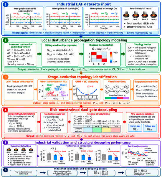
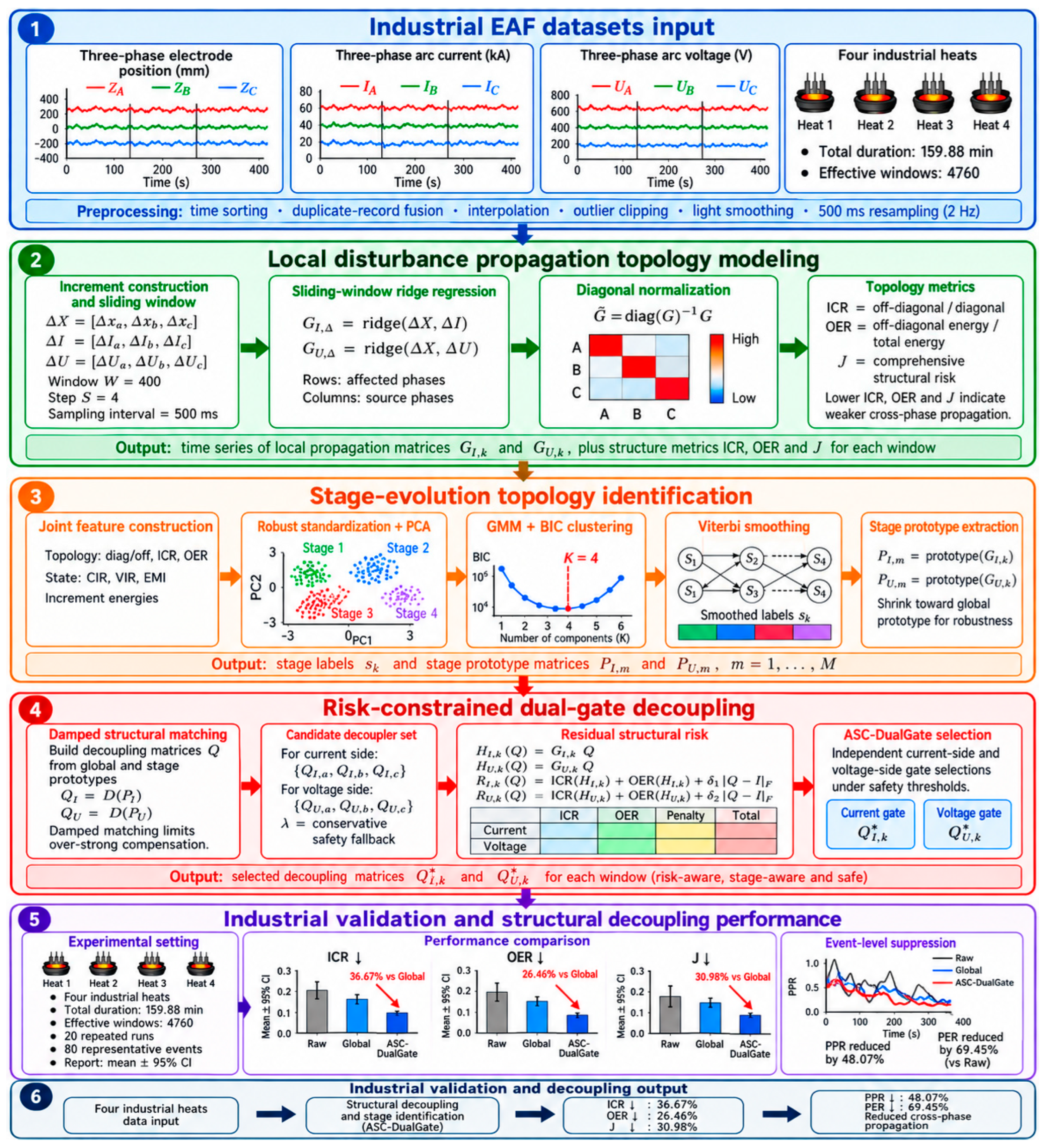
Figure 1 summarizes the complete analysis chain from archived plant measurements to local propagation maps, coarse stage priors, risk-constrained candidate selection, and evaluation. The diagram is an original schematic prepared for this study; none of its panels reproduces or adapts a previously published figure. In Figure 1, the labels ‘industrial validation’ and ‘experimental setting’ refer to offline replay of industrial records, not to online actuation of the proposed compensation on the furnace.
Figure 1.
Original schematic of the proposed closed-loop propagation-map analysis and risk-constrained dual-gated compensation workflow; industrial data results are offline replay.
2.1. Measurement Data and Modeling
The data are archived field measurements from four heats of the same 75 t three-phase AC EAF while its original electrode regulator was operating. No ASC-DualGate command was sent to the furnace. The records contain the equivalent positions of electrodes A-C, phase arc currents, and phase arc voltages. The four heats comprise 19,193 raw records over 159.88 min; 19,190 records remain after timestamp and validity checks. Thus, the dataset supports retrospective structural identification and replay, rather than a prospective online controller trial.
The equivalent electrode-position vector, arc-current vector, and arc-voltage vector are defined below. To remove the visual ambiguity between lowercase l and the numeral 1, the position symbol is standardized as uppercase L in Equations (1), (4), (8), and (29):
The corresponding first-order incremental variables are constructed as:
The four heats contribute 7519, 3786, 3727, and 4161 raw records, respectively. After preprocessing, the corresponding valid record counts are 7518, 3786, 3726, and 4160; the durations are 62.64, 31.54, 31.04, and 34.66 min. Sliding-window segmentation yields 1870, 937, 922, and 1031 windows (4760 in total), as summarized in Table 1.
Table 1.
Data size and operating-condition characteristics of the four industrial heats.
2.2. Data Preprocessing and Sliding-Window Construction
Records are sorted by timestamp, duplicate timestamps are fused, and all channels are resampled at 500 ms (2 Hz), with time interpolation for isolated gaps. Each channel is clipped to its 0.5th and 99.5th percentiles, followed by a centered two-sample moving average. First differences are then computed. These settings are fixed for all heats and methods.
The equivalent electrode positions, arc currents, and arc voltages of the three phases are uniformly time-aligned, and sliding-window samples are constructed from the incremental variables. Let the window length be W and the sliding step be S; the sample set corresponding to the k-th window is defined as:
The fixed settings are W = 40 samples (20 s) and S = 4 samples (2 s); thus, adjacent windows overlap by 90%. This overlap improves temporal resolution but makes neighboring windows statistically dependent; the confidence intervals reported later must, therefore, not be interpreted as though all 4760 windows are independent observations. For the k-th window, the input matrix is defined as:
Continuous sliding of the window yields a time series of local disturbance propagation structures that evolves with the operating process.
2.3. Local Disturbance Propagation Matrix Estimation
Within each sliding window, the local mappings from the three-phase electrode-position increments to the arc current increments and arc voltage increments are established separately:
Taking the current side as an example, its local disturbance propagation matrix is expressed as:
In each propagation matrix, rows denote affected phases and columns denote electrode-motion source phases. Previous studies have investigated recursive identification of EAF electrode-regulator systems [28] and time-varying EAF modeling [29]. Ridge regression stabilizes the correlated three-input fit [30], while the closed-loop interpretation follows established cautions on feedback-data identification [31,32]. Related recurrent data-driven EAF modeling demonstrates the value of learning nonstationary behavior [24], but the present 3 × 3 matrices are local propagation summaries rather than sequence predictors:
Taking the current side as an example, its closed-form solution is given by:
The voltage-side propagation matrix is solved in the same form. Estimation over consecutive windows yields the sequences of local disturbance propagation matrices:
Because the incumbent regulator was active during acquisition, electrode-position increments can be correlated with unmeasured electrical disturbances. Ridge regularization controls variance but does not remove this feedback-induced bias; the resulting G matrices are, therefore, used only as closed-loop equivalent propagation maps, which are examined in Section 2.6.
2.4. Normalization of Local Propagation Structures and Structural Indicators
To reduce the influence of variations in the in-phase response magnitude on inter-phase propagation comparison, diagonal normalization is applied to the local propagation matrices.
The normalized propagation matrix is:
To quantitatively evaluate the degree of inter-phase coupling in the propagation matrix, the inter-phase coupling ratio (ICR) is defined as:
A larger ICR indicates stronger off-diagonal propagation relative to the in-phase response. The off-diagonal energy ratio (OER) is defined as:
The OER denotes the proportion of off-diagonal energy in the total matrix energy. Considering the residual propagation intensity on both the current and voltage sides, the overall structural risk of the k-th window is defined as:
A smaller value indicates weaker overall residual inter-phase propagation on the current and voltage sides in the current window. For a given heat or decoupling method, the average overall structural risk is defined as:
These indicators provide the basis for the subsequent stage-aware propagation structure identification, stage prototype extraction, and risk-constrained dual-gated decoupling.
2.5. Structural Indicators and Operating-State Indicators
The current imbalance ratio, voltage imbalance ratio, and electrode motion intensity are computed to characterize three-phase electrical asymmetry and electrode-regulation burden [6,23,33]. The current imbalance ratio of the k-th window is defined as:
The corresponding voltage imbalance ratio is defined as:
The electrode motion intensity is defined as:
The operating-state indicators support stage identification and help to interpret variations in the propagation structure under different operating conditions.
2.6. Closed-Loop Interpretation and Identification-Bias Diagnostics
In feedback operation, disturbances affect current and voltage directly and also modify electrode motion through the incumbent controller. Consequently, the regression input may be correlated with its error; thus, neither the persistence of excitation nor unbiased open-loop plant identification is guaranteed [31,32]. In this paper, G denotes an operating policy-dependent closed-loop association. It must not be interpreted as physical admittance, a causal graph, or a controller-invariant sensitivity. This restricted interpretation is, nevertheless, relevant for auditing candidate compensation superimposed on the same incumbent loop.
Three diagnostics quantify the identification conditions. Defining silent and active windows by the lowest and highest quartiles of electrode-motion energy, active-window electrical-increment energy is 2.97–6.89 times the silent-window level. Across heat-side combinations, the median absolute Spearman correlation between electrode increments and ridge residuals is 0.108–0.155. A lag-2 electrode-increment instrument preserves 65.1–70.3% mean off-diagonal sign agreement, with a median first-stage R2 of 0.156–0.189. These results provide a directional robustness check on the estimated propagation structure, while the limited first-stage strength means that the IV diagnostic is not used to claim unbiased plant identification. Command-based instruments are unavailable in the present records and should be incorporated in future prospective trials.
3. Stage-Aware Disturbance Propagation Structure Identification
Because the EAF operating state exhibits pronounced local time-varying behavior, inter-phase propagation intensity, propagation direction, and electrical response characteristics may vary across windows. To characterize these recurrent local structural variations, the propagation matrices of consecutive windows are organized into several statistical propagation stages, and current-side and voltage-side stage prototype matrices are extracted from each stage.
3.1. Construction of Stage Identification Features
The local disturbance propagation matrix reflects how three-phase electrode motion within a window propagates to the current-side and voltage-side responses. For the k-th window, a joint observation vector composed of propagation-structure features and operating-state features is constructed:
To further reflect the variation intensity of the electrical quantities and electrode motion within a window, the current increment energy is defined as:
After robust feature standardization, principal component analysis is applied to reduce feature redundancy [34]. The dimensionality-reduced feature vectors are then used for statistical propagation-stage identification.
3.2. Propagation Stage Identification Based on the Gaussian Mixture Model
The disturbance propagation state during EAF operation generally varies gradually, and fixed boundaries between propagation states cannot be preset reliably. A Gaussian mixture model is, therefore, used for probabilistic clustering of the window-level features [35]. Its probability distribution is expressed as:
According to Bayes’ rule, the posterior probability that the k-th window belongs to the m-th propagation stage is:
The initial propagation stage label of a window is obtained from the maximum posterior probability:
The operational stage-prior model searches M = 2–3 Gaussian components by BIC, retains components with at least 4% of the windows and at least 60 windows, and applies a Viterbi switching penalty of 1.2 after robust standardization and eight-component PCA. This deliberately coarse partition is an organizational prior, not evidence that the furnace has exactly two or three physical stages. The Bayesian information criterion is defined as:
The selection of the number of propagation stages can be expressed as:
Components with an excessively small sample proportion or too short a duration are merged into the nearest neighboring stage in the feature space to reduce fragmented stage labels.
3.3. Temporal Consistency Correction of Stage Labels
Because the local operating state of the EAF generally has temporal persistence, a temporal consistency correction method based on Viterbi dynamic programming is introduced. The optimization objective for the stage sequence is defined as [36], where τv denotes the stage-switching penalty coefficient:
After solving by Viterbi dynamic programming, the corrected stage label of the k-th window is:
The temporal consistency correction suppresses high-frequency label switching caused by local noise, transient anomalies, and weakly separable windows, while preserving the main propagation-state transitions. It, therefore, provides a stable basis for extracting stage prototype matrices.
3.4. Stage Prototype Matrix Extraction
Representative current-side and voltage-side stage prototype matrices are extracted from the local propagation matrices contained in each stage. The set of windows belonging to the m-th propagation stage is defined as:
The current-side and voltage-side prototype matrices corresponding to the m-th stage are defined as:
Taking the current side as an example, the deviation of the k-th window within the m-th stage relative to the stage median structure is defined as:
Within each stage, matrices outside the central 80% of Frobenius distances from the median are excluded before taking the robust median. The stage prototype is then shrunk toward the global prototype with , where nm is the stage sample count. This continuous shrinkage replaces an unspecified qualitative correction and prevents small stages from producing an unconstrained decoupler. The shrunken stage prototypes are:
4. Risk-Constrained Dual-Gated Structural Decoupling Method
This section constructs the structural decoupling matrices and proposes a risk-constrained dual-gated selection mechanism. The mechanism incorporates the global candidate, stage-aware candidate, and safe-fallback candidate into a common candidate set, computes the post-compensation residual structural risk separately on the current and voltage sides, and selects the constraint-satisfying decoupling matrix with the lowest risk.
4.1. Construction of Structure-Matching Decoupling Matrices
To attenuate inter-phase disturbance propagation induced by three-phase electrode motion, the corresponding structural decoupling matrices are constructed. For any local propagation matrix G, the post-compensation equivalent propagation matrix is expressed as:
The post-compensation propagation matrix is encouraged to approach a diagonal map. The damped least-squares construction is a regularized structure-matching transformation related to established multivariable interaction and furnace-decoupling ideas [22,37,38,39,40,41], rather than a new physical short-network model. Its damping and intensity limits are stated explicitly in Section 5.2:
The closed-form solution is:
The global decoupling matrices are constructed separately:
For the m-th propagation stage, the stage-aware decoupling matrix is constructed using the shrunken stage prototype matrix:
The global decoupling matrix reflects the relatively stable average propagation relationship over the heat, whereas the stage-aware decoupling matrix reflects the local structural characteristics of the corresponding statistical propagation stage.
4.2. Comparative Decoupling Strategies
To evaluate the roles of stage-aware propagation-structure information, risk screening, and the safe-fallback mechanism, representative decoupling methods are used as comparative strategies under the same local propagation matrices and evaluation indicators.
The uncompensated method applies no structural transformation to the three-phase electrode input channels:
The global decoupling method adopts a fixed global decoupling matrix across all windows:
The static interaction decoupling method (SID) constructs a fixed interaction compensation matrix from the off-diagonal part of the global propagation structure:
The coupling-intensity adaptive decoupling method (FSD) adaptively adjusts the compensation intensity according to the local inter-phase coupling degree of the current window:
ALID is an adaptive PSD-type local decoupling baseline. In the implementation used to generate the comparison results, a locally high-damped structure-matching matrix is first constructed from the current-window propagation matrix and then conservatively blended with the identity matrix:
Here, the nominal ALID blending coefficient is αA = 0.45 and the local damping is κloc = 0.85. To avoid excessively strong compensation from the local matrix, the normalized deviation of the compensation matrix from the identity matrix is constrained. If the nominal αA violates the constraint, αA is multiplied successively by 0.75 until the constraint is satisfied or αA reaches 0.05:
The direct stage-switching method (HardStage) directly adopts the corresponding stage-aware decoupling matrix according to the current stage label:
The confidence soft-fusion method (ConfidenceSoft) performs a weighted fusion between the global decoupling matrix and the stage-aware decoupling matrix according to the stage posterior confidence:
The definitions and roles of the different structural decoupling strategies are summarized in Table 2.
Table 2.
Definitions and roles of the different structural decoupling strategies.
4.3. ASC-DualGate Risk-Constrained Dual-Gated Decoupling
Selection is performed independently for s ∈ {I, U}. Let Qs,g and denote the global and current-stage matrices, ck the GMM confidence, and Bs,k(w) their convex blend. The stage weight w(Q) is 0 for Qs,g; min(ck,0.85) for the confidence blend; 0.25, 0.50, or 0.75 for the fixed blends; 1 for ; and the discrete fallback blend μ for a fallback candidate. The complete normal-candidate family is:
Safe fallback is generated only after the best normal candidate fails the side-specific trigger. For side s ∈ {I, U}, let be that normal candidate and let Dκ(G) denote the structure-matching operator defined by Equation (45) and parameterized by damping coefficient κ. With local damping κloc = 0.85, the local matrix and the finite fallback family are constructed as follows:
A fallback is admissible when cond(Q) ≤ 30 and . To prevent the retrospective structural metric from being driven artificially to zero, residual ICR must remain at least 0.30 of Raw on the current side and 0.18 of Raw on the voltage side; if all local blends violate a bound, 0.80Qn + 0.20I is used. This floor is an offline anti-degeneracy safeguard, not a plant safety limit:
For Hs,k(Q) = Gs,kQ, define . The same residual-risk score is used for both sides. The trigger constants in Equation (62) are (aI, bI) = (0.94, 1.06) and (aU, bU) = (0.40, 1.04):
The lowest-score normal candidate is selected first. Only when its score exceeds Ts,k is the admissible fallback family evaluated. Let be its lowest-score member; it replaces the normal choice only when the score decreases by more than 0.015. The resulting rule is:
The final compensated current-side and voltage-side propagation matrices are:
In ASC-DualGate, stage identification and stage prototypes are used to construct decoupling candidates that match the local propagation state, whereas residual structural-risk screening determines whether a candidate yields a low residual structural risk on the current or voltage side of the current window.
4.4. Decoupling Performance Evaluation Indicators
The residual inter-phase coupling ratio and off-diagonal energy ratio are computed from the compensated current-side and voltage-side propagation matrices:
On this basis, the post-compensation overall structural risk and its heat-averaged value are defined as:
The ICR evaluates off-diagonal propagation intensity relative to the in-phase response, the OER evaluates the proportion of off-diagonal propagation energy in the total matrix energy, and J represents the combined residual structural risk on the current and voltage sides. Smaller values indicate weaker inter-phase disturbance propagation after compensation.
5. Experimental Validation and Result Analysis
5.1. Experimental Validation Scheme
Section 5 reports offline structural replay on the four archived industrial heats; it is not an online furnace experiment. Seeds 42–61 affect only GMM initialization and the resulting labels, prototypes, and gate sequences. Raw and Global, the preprocessing, and the measured records are not randomly resampled. For seed-level quantities, the reported interval is . Because W = 40 and S = 4 create 90% overlap, these intervals describe algorithmic stability across initializations, not independent-window sampling uncertainty.
5.2. Dataset and Experimental Parameters
The numerical settings used in every reported comparison are: ridge λ = 3.0; local clipping z = 4.0; local weight c = 3.0; matrix smoothing γ = 0.50; PCA dimension 8; GMM M = 2–3; Viterbi stage-switching penalty τv = 1.2; minimum stage ratio 0.04; minimum stage-window number 60; prototype pseudo-count 120; global, stage and local structure-matching damping κg = 0.35, κs = 0.45, and κloc = 0.85; matrix-element clip ±2.5; compensation-deviation penalty 0.035; and overall-J weights (0.38, 0.22, 0.28, 0.12) for (ICRI, OERI, ICRU, OERU). Baseline settings are SID strength 0.42; FSD maximum strength 0.55 and sensitivity 0.35; and ALID nominal blending coefficient αA = 0.45, using the local structure-matching matrix with κloc = 0.85 and normalized compensation-deviation limit qmax = 1.35; if the limit is exceeded, αA is reduced by a factor of 0.75 down to a minimum of 0.05. For ASC-DualGate, the fallback-candidate condition-number limit is 30, the normalized compensation-intensity limit is 1.8, the fallback blend levels are μ ∈ {0.20, 0.35, 0.50, 0.65, 0.80}, and the replacement margin is 0.015. These nominal values are fixed engineering settings of the analyzed implementation and are frozen across all heats; they were not re-optimized for individual test heats and are not claimed to be a unique data-driven optimum. Section 5.11, therefore, reports bounded perturbation, interaction, and objective-weight scans to quantify sensitivity to these fixed choices.
Table 3 summarizes the coarse M = 2–3 statistical partitions and the detected events. The stages are recurring clusters of closed-loop propagation features used to generate candidate priors; they are not assigned to melting, refining, or any other metallurgical stage, and no such physical interpretation is claimed.
Table 3.
Stage identification and disturbance event statistics for the four industrial heats.
5.3. Results of Stage-Aware Propagation Structure Identification
The statistical propagation stages in different heats are identified using the local propagation matrices and operating-state features. After robust standardization and principal component analysis, the window features are fed into the GMM, and the final stage labels are obtained through temporal consistency correction.
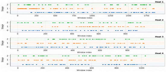
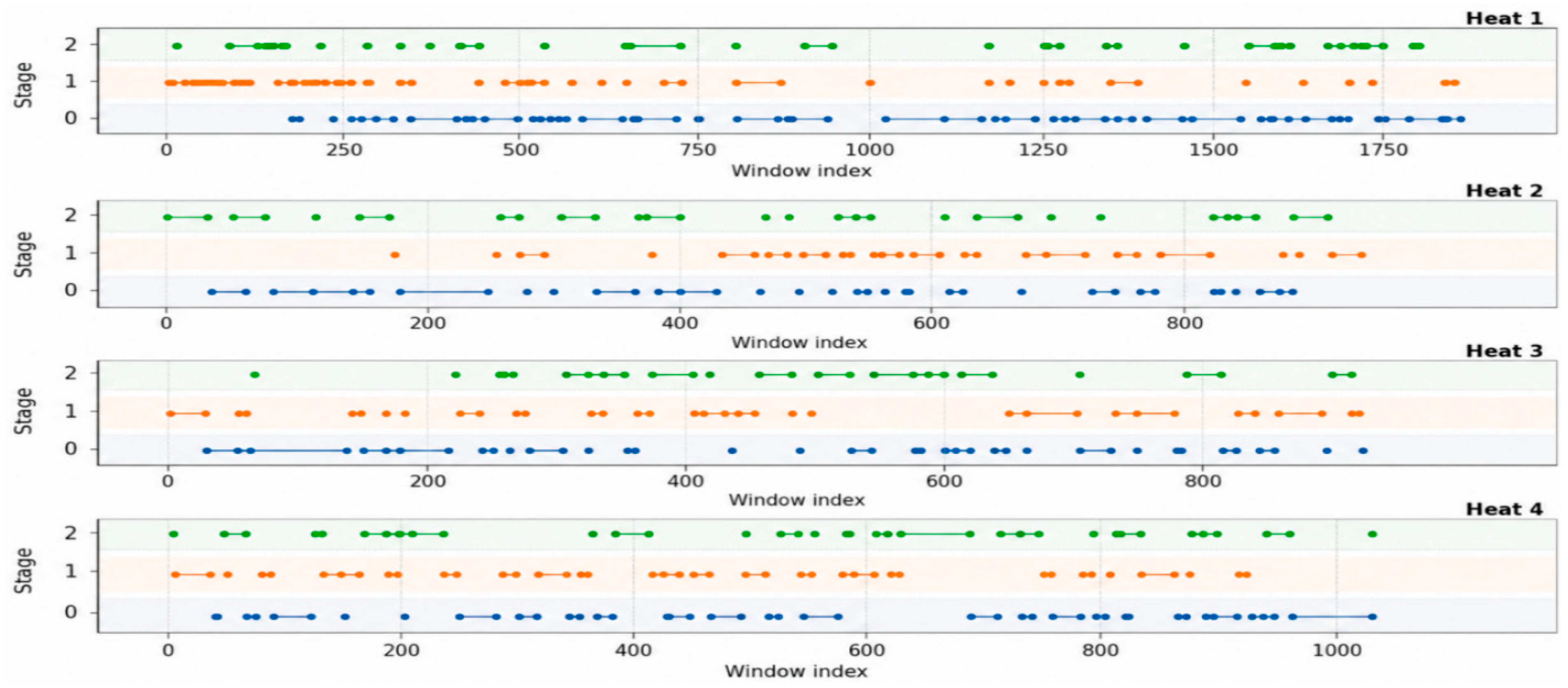
Figure 2 presents the window-level statistical propagation-stage sequences of the four industrial heats. After temporal consistency correction, each stage exhibits temporal continuity, while transitions among the main propagation states are preserved. The stage durations and switching patterns differ across heats, indicating that the local propagation structure during three-phase electrode regulation varies with the operating state.
Figure 2.
Temporal evolution of the propagation-stage labels for the four industrial heats.
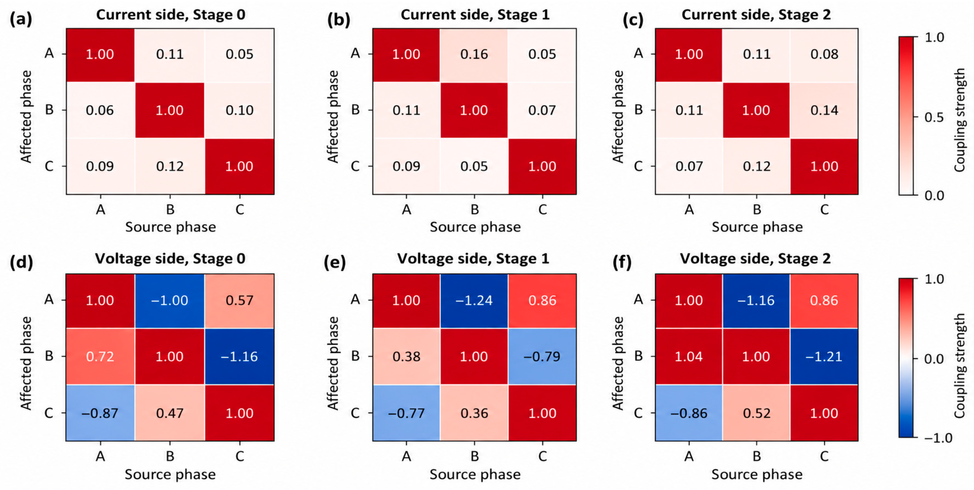
Figure 3 shows the current-side and voltage-side prototype matrices of the statistical propagation stages in Heat 1. The diagonal elements of each stage prototype preserve the dominant in-phase response, whereas the off-diagonal elements differ in intensity and direction, indicating that the inter-phase disturbance propagation pattern varies with the statistical propagation stage. The voltage-side prototypes exhibit more pronounced off-diagonal propagation and sign changes, suggesting that the voltage response is more susceptible to the combined influence of the common three-phase supply network, short-network mutual coupling, and electrical paths within the furnace.
Figure 3.
Coupling strength matrices between source and affected phases at different stages: (a) current-side coupling strength at Stage 0; (b) current-side coupling strength at Stage 1; (c) current-side coupling strength at Stage 2; (d) voltage-side coupling strength at Stage 0; (e) voltage-side coupling strength at Stage 1; (f) voltage-side coupling strength at Stage 2.
5.4. Overall Performance Comparison of Different Decoupling Methods
To evaluate the structural decoupling performance of ASC-DualGate, it is compared with representative methods. All methods are applied to the same local propagation matrices and evaluated using the same structural indicators.
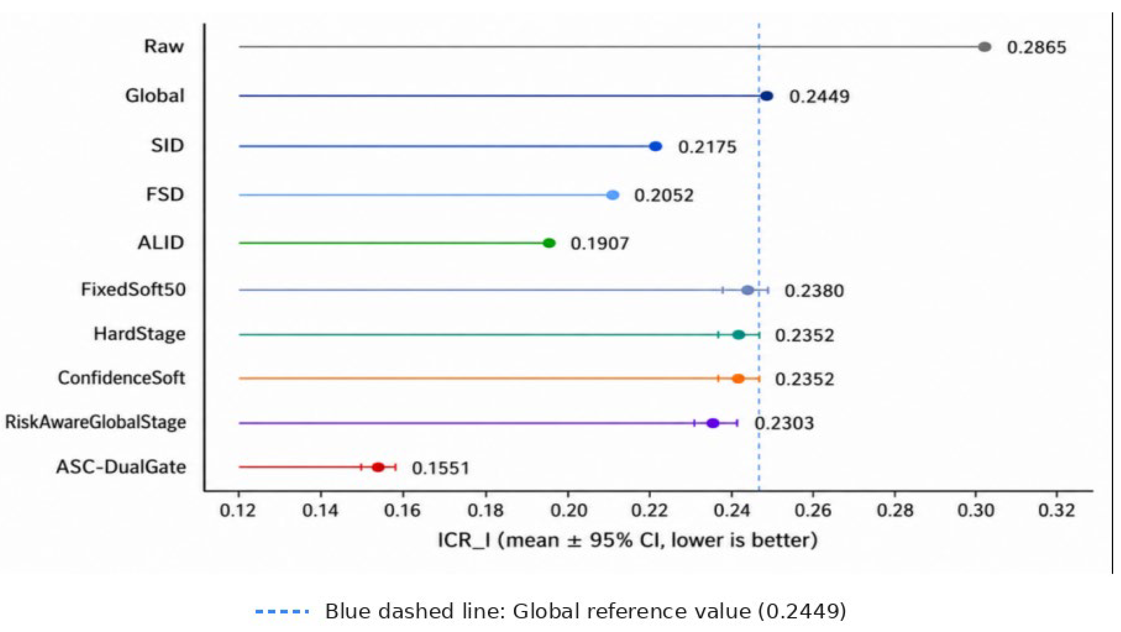
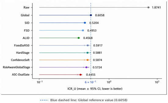
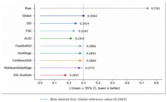
Table 4 and Figure 4, Figure 5 and Figure 6 compare mechanism-internal residual risks computed on the same windows used to estimate the local maps. Global confirms that an exploitable average propagation association exists. Improvements beyond Global should be read as retrospective structural replay, not as measured closed-loop production gains.
Table 4.
Average structural decoupling performance of different methods over the four industrial heats.
Figure 4.
Current-side residual inter-phase coupling ratio of different decoupling methods.
Figure 5.
Voltage-side residual inter-phase coupling ratio of different decoupling methods.
Figure 6.
Overall structural risk of different decoupling methods.
Relative to Global, SID, FSD, and ALID further reduce the overall structural risk, with J decreasing by 11.18%, 13.63%, and 17.97%, respectively. This result indicates that local structural information can provide stronger adaptive compensation beyond fixed global decoupling. FixedSoft50, HardStage, and ConfidenceSoft also yield limited improvements, suggesting that stage-propagation prototypes contain useful compensation information, but that relying only on the stage matrix or stage confidence is insufficient for full adaptation to the current local window.
ASC-DualGate has the lowest same-window J among the compared methods. Separate gates enable the current and voltage candidates to differ, while the same-window comparison uses the current estimated map for both candidate selection and structural scoring. Section 5.10, therefore, introduces a temporally separated, leave-one-heat-out test to assess transfer beyond the same-window structural evaluation.
5.5. Per-Heat Structural Decoupling Results
To evaluate the stability of the proposed method under different industrial operating conditions, the overall structural risk of Raw, Global, RiskAwareGlobalStage, and ASC-DualGate is computed for each heat separately.
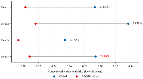
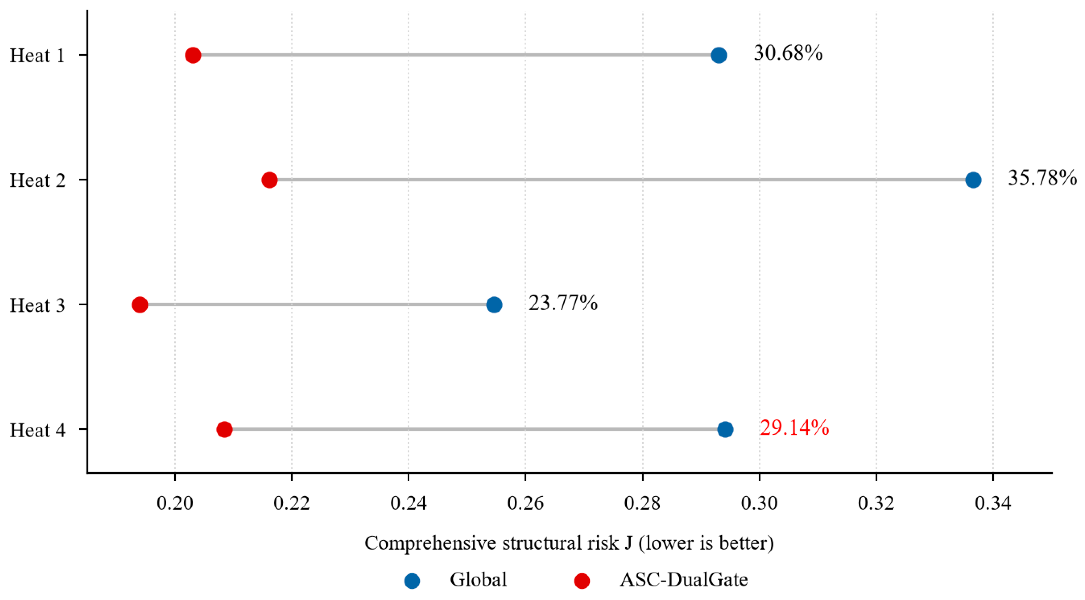
Table 5 and Figure 7 use the same values: the reductions from Heat 1 to Heat 4 are 30.68%, 35.78%, 23.77%, and 29.14%, respectively. The former 29.40% label in Figure 7 was a transcription error; . All four same-window comparisons favor ASC-DualGate, but they remain within-sample structural evaluations on one furnace.
Table 5.
Overall structural risk of different decoupling methods in each industrial heat.
Figure 7.
Same-window structural risk of Global and ASC-DualGate by heat; the Heat 4 reduction is 29.14%.
5.6. Ablation Experiments
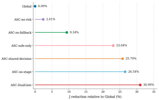
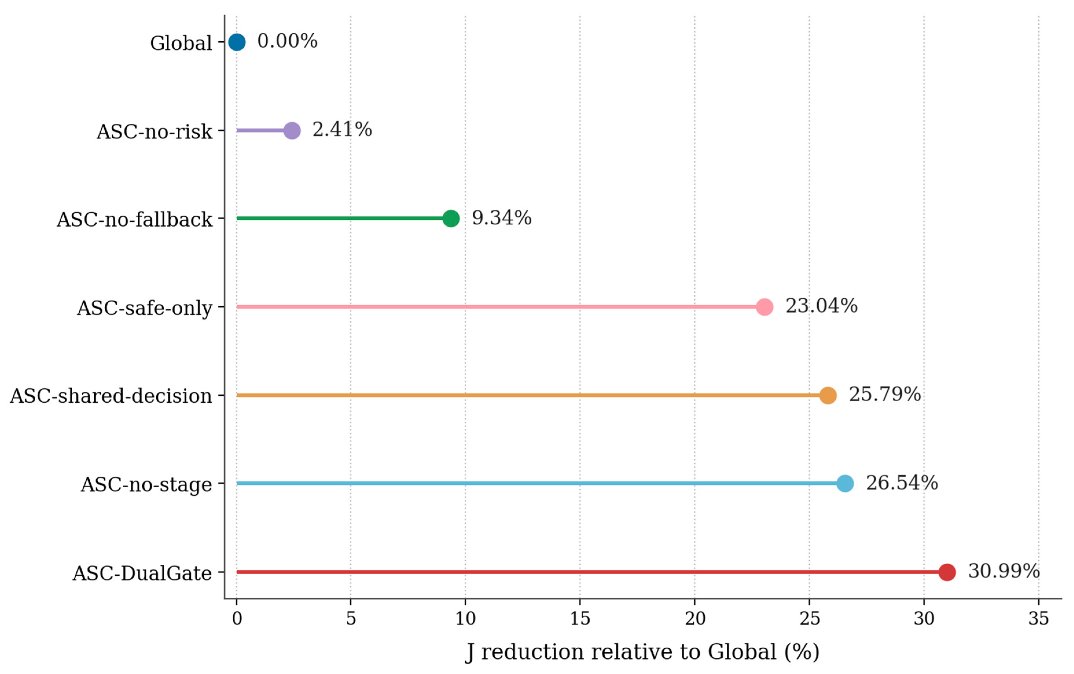
To analyze the roles of the components in ASC-DualGate, ablation experiments are designed. ASC-no-risk removes local residual-risk screening; ASC-no-fallback removes the safe-fallback candidate; ASC-safe-only retains only the safe-fallback candidate; ASC-no-stage removes the stage-aware candidate; and ASC-shared-decision requires the current and voltage sides to share the same candidate-selection result. Figure 8 illustrates the ablation results, and Table 6 provides the corresponding numerical comparisons.
Figure 8.
Ablation results of the overall structural risk of ASC-DualGate.
Table 6.
Ablation results of ASC-DualGate.
The ablation results require a qualified interpretation. Relative to Global, the complete method reduces J by 30.99% in the rounded ablation table, while ASC-no-stage and ASC-safe-only still reduce J by 26.54% and 23.04%. Removing risk screening or fallback limits the reduction to 2.41% and 9.34%, respectively; forcing a shared current/voltage decision gives 25.79%. The incremental gain of the full method over ASC-no-stage is 6.06% of the latter’s J; its gain over the shared-decision variant is 7.01%. Therefore, risk screening and bounded fallback account for most of the aggregate benefit; stage priors and independent gates provide smaller, non-additive refinements instead of a sole source of improvement.
5.7. Analysis of the ASC-DualGate Candidate Selection Mechanism
To further analyze the internal working mechanism of dual gating, the selection frequencies of the global candidate, stage-aware candidate, and safe-fallback candidate are counted separately for the current and voltage sides in the four heats.
Table 7 shows frequent fallback use, including 49.07% on the Heat 1 current side and 32.50–49.97% across the other current-side heats. Fallback is invoked when the best global/stage-family candidate does not clear the side-specific risk trigger. This pattern is consistent with substantial within-heat variation in the estimated local propagation structure and with uncertainty around statistical-stage boundaries, although Table 7 alone does not distinguish these mechanisms. Because fallback is a bounded blend rather than identity or full local inversion, its selection frequency indicates that conservative local correction contributes materially to the overall decision process. The stage prior should, therefore, be interpreted as a complementary candidate source rather than the sole driver of performance.
Table 7.
Candidate selection frequencies of ASC-DualGate on the current and voltage sides.
5.8. Event-Level Disturbance Propagation Analysis
Events are detected from current-increment energy. Windows at or above the heat-specific 90th percentile are scanned chronologically, and accepted centers must be separated by at least eight window steps (16 s). At most, 25 candidates, and at least 8 candidates are retained per heat, yielding 25, 19, 18, and 18 events (80 total). Each event is represented by its 40-sample, 20 s window. Centers exactly eight steps apart leave at most 4 s of window overlap; no overlapping center is counted twice.
For current-side H = GQ, the dominant source phase m is the column with the largest sum of absolute off-diagonal entries, with R = {A, B, C}\{m}: ; ; .
The dominant phase and event centers are defined once per event and reused across methods. Results are first averaged across the 20 GMM seeds for each heat-event-method unit. The 95% event intervals are then obtained from 5000 bootstrap resamples of the 80 event units. PPR, PER, and MPR are not included in the candidate-selection risk; therefore, they are evaluation criteria rather than gate inputs.
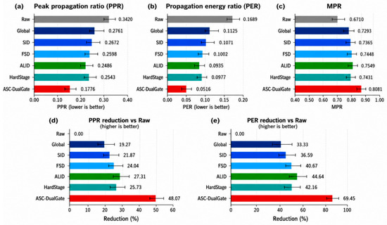
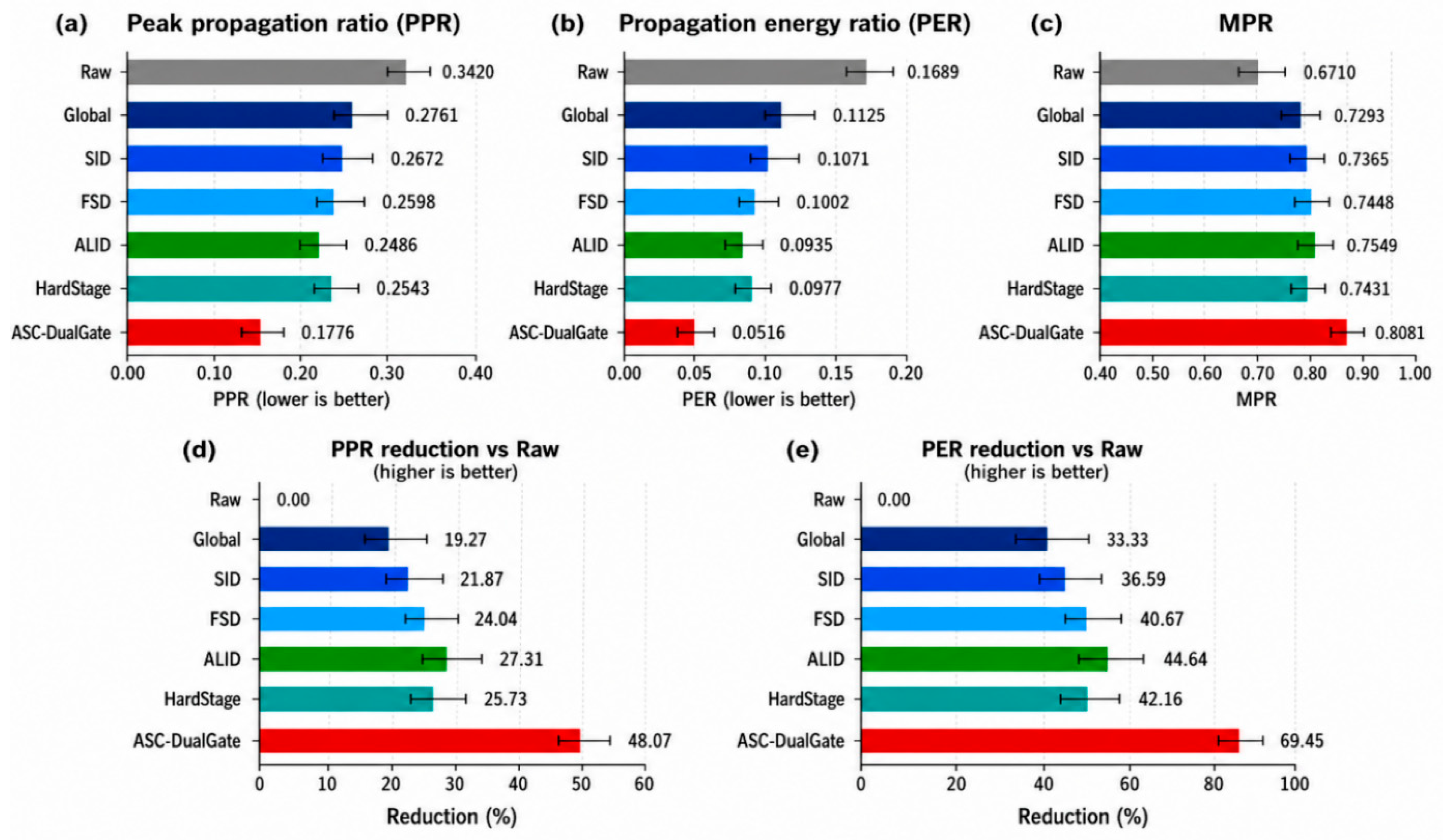
Table 8 and Figure 9 show that ASC-DualGate has the lowest event-unit PPR and PER. Relative to Raw, PPR changes from 0.3420 to 0.1776 (48.07% reduction) and PER from 0.1689 to 0.0516 (69.45% reduction). These values quantify structural propagation within detected windows; they are not measurements of furnace productivity, energy consumption, or electrode wear.
Table 8.
Comparison of event-level propagation indicators of different decoupling methods.
Figure 9.
Comparison of different methods in terms of (a) peak propagation ratio (PPR); (b) propagation energy ratio (PER); (c) MPR; (d) PPR reduction relative to the Raw method; and (e) PER reduction relative to the Raw method. Error bars indicate the uncertainty associated with the corresponding measurements.
Global, SID, FSD, ALID, and HardStage all reduce event-level propagation intensity to varying degrees; however, fixed compensation, local decoupling, and hard stage partitioning have limited ability to adapt to changing furnace conditions. Through dual-gated risk screening and safe fallback, ASC-DualGate enables the stage-aware decoupling matrix to participate in correction only when the compensation direction is reliable, thereby achieving more stable propagation suppression.
Meanwhile, the MPR of ASC-DualGate increases to 0.8081, indicating that it does not simply suppress the overall three-phase response. Instead, it suppresses non-dominant-phase propagation while preserving the dominant-phase response structure, thereby concentrating the disturbance response in the dominant-phase channel.
5.9. Analysis of Typical Disturbance Events
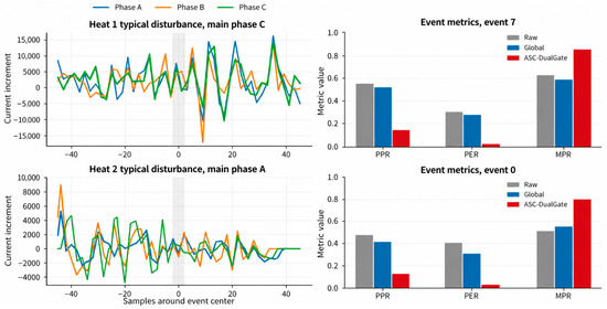
Representative disturbance events from Heat 1 and Heat 2 are selected for time-domain analysis.
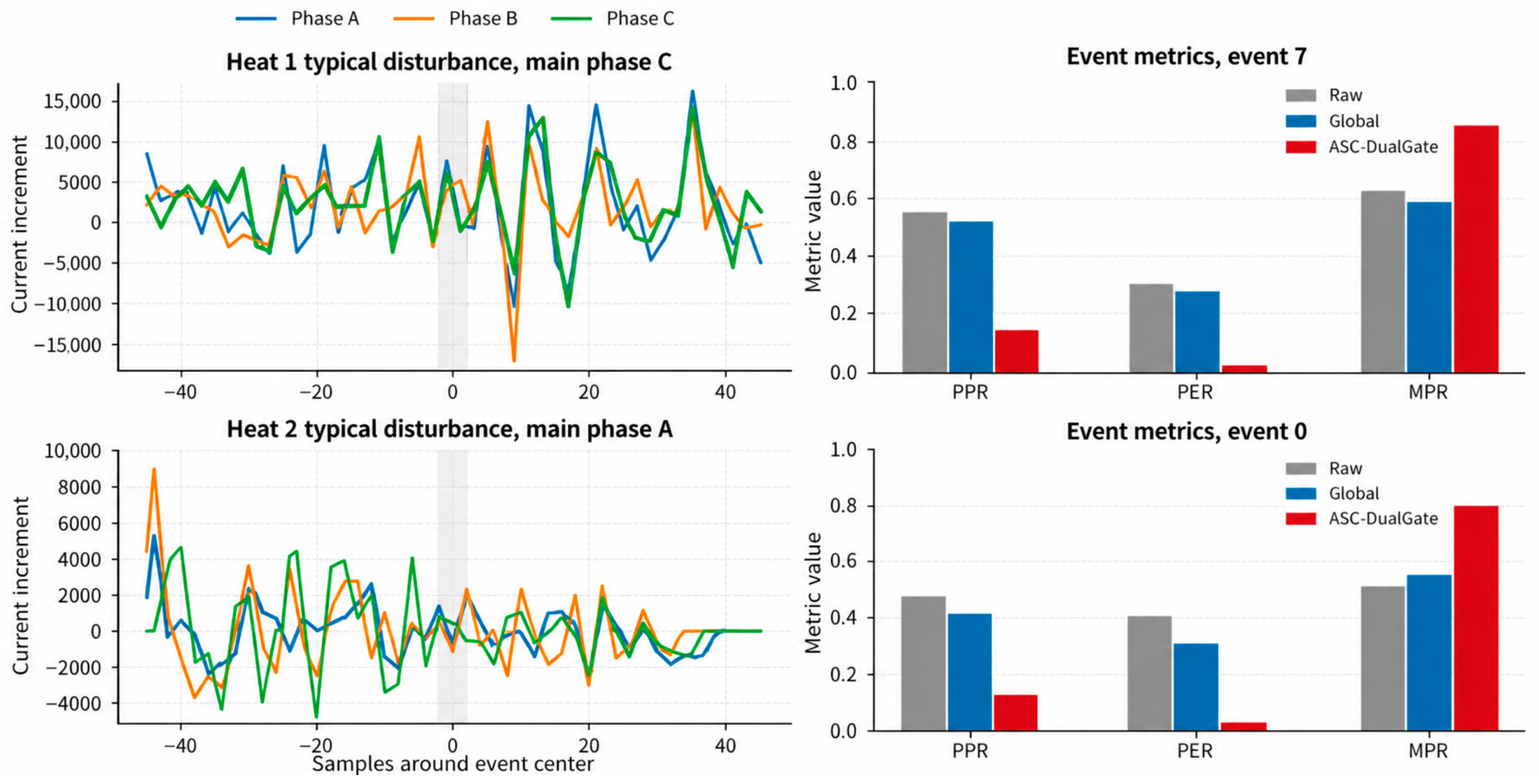
Figure 10 presents the three-phase current increments near representative disturbance events, together with the event-level propagation indicators of Raw, Global, and ASC-DualGate. Compared with Raw and Global, ASC-DualGate achieves lower PPR and PER, while maintaining a higher MPR, indicating that it attenuates the non-dominant-phase peak response and propagation energy while preserving the main disturbance response.
Figure 10.
Three-phase current increments and event-level indicators of representative disturbance events in Heat 1 and Heat 2.
The representative events in Heat 1 and Heat 2 differ in propagation direction, peak magnitude, and duration. Nevertheless, ASC-DualGate exhibits consistent suppression of non-dominant-phase propagation in both event types. This result indicates that the stage-aware candidate and dual-gated selection adjust the compensation according to different local propagation structures.
Taken together, Section 5.3, Section 5.4, Section 5.5, Section 5.6, Section 5.7, Section 5.8 and Section 5.9 establish same-window mechanism behavior. Because the same local map enters candidate selection and structural scoring, these results are interpreted as mechanism-level retrospective replay rather than as an independent temporal-transfer test. Section 5.10, therefore, provides a temporally separated leave-one-heat-out evaluation.
5.10. Leave-One-Heat-Out Future-Window Evaluation
A leakage-controlled replay evaluates the exact ASC-DualGate pipeline. In each outer fold, signal and feature clipping, robust scaling, PCA, GMM selection by BIC, Viterbi mapping, global/stage prototypes, and decouplers are fitted only on the other three heats for each seed 42–61. On the held-out heat, causal prefix Viterbi supplies the stage state and confidence. A 20 s past window estimates Gt and the unchanged Equations (57)–(64) select Qt; Qt is then frozen and evaluated on the immediately following nonoverlapping 20 s window through Gt + 1Qt. The protocol yields 472 held-out episodes. Seed results are averaged within each episode before inference; thus, the physical episodes, rather than the 9440 seed-episode rows, are the statistical units. Table 9 summarizes the leave-one-heat-out future-window evaluation results.
Table 9.
Exact-algorithm leave-one-heat-out past-to-future replay. Aggregate improvement is 100(mean JGlobal-mean JASC)/mean JGlobal; positive values indicate lower future-window J for ASC-DualGate, whereas negative values indicate higher future-window J.
The temporally separated evaluation is substantially more stringent than the same-window structural replay. Heat 1 retains a 7.13% aggregate reduction in future-window J, whereas the remaining held-out heats show higher future-window J for ASC-DualGate under this one-window-ahead protocol. At the pooled level, Global and ASC-DualGate yield J = 0.3160 and 0.3207, respectively, corresponding to an aggregate improvement of −1.49% by the predefined ratio. Across the 472 physical episodes, the mean episode-wise relative change is −6.44% (5000-resample bootstrap 95% CI, −8.74% to −4.32%), the median change is −1.45%, and 44.70% of episodes have lower J with ASC-DualGate (Wilcoxon p = 4.15 × 10⁻⁴; rank-biserial effect (ASC minus Global): 0.190). Stage and fallback candidates are selected on at least one side in 58.58% and 64.98% of episodes, respectively. These results indicate that the structural advantage observed in same-window replay is sensitive to short-term operating-condition changes and is, therefore, used to define the present generalization boundary rather than to support a universal cross-window transfer claim.
5.11. Hyperparameter Selection and Multi-Parameter Robustness
Ridge multipliers {0.1, 0.3, 1, 3, 10} retain 74.7–86.9% current-side and 92.7–99.1% voltage-side off-diagonal signs relative to the nominal estimate across the four heats. A ±50% trigger scan shows that the advantage threshold is influential: J ranges from 0.1596 to 0.2435 while fallback frequency changes from 83.10% to 8.28%. In contrast, the fallback-use penalty scan changes J by less than 0.00001. A 3 × 3 damping-penalty interaction grid gives J = 0.1970–0.2074, and alternative current-heavy, equal, and voltage-heavy J weights retain a 28.74–32.88% same-window reduction relative to Global.
A formal multi-objective optimizer is not fitted because four heats from one furnace do not provide an independent calibration population; optimizing several objectives on this sample would increase overfitting. Instead, nominal settings are treated as frozen engineering choices and the interaction and objective-weight scans expose their sensitivity. With additional furnaces, future work should estimate a Pareto set over structural risk, current/voltage imbalance, actuator travel, condition number, and fallback frequency on a calibration cohort, and test it prospectively.
6. Simulation Validation
6.1. Simulation Platform and Validation Scheme
The reduced simulator contains a 650 V three-phase source; a short-network matrix with diagonal impedances (0.0038, 0.0040, 0.0039) Ω and mutual terms (0.00145, 0.00115, 0.00135) Ω; phase arc resistances (0.00250, 0.00260, 0.00255) Ω; and an arc-voltage relation with a 175 V offset and a 3.15 V/mm slope with an approximately 20 mm nominal length [8,11,27,42]. The actuator is first order, with 0.0538 s time constant, 25.26 mm/s velocity limit, and 0.135 mm/s deadband. PI gains are Kp,I = 42.08, Ki,I = 4.98, Kp,U = 20.08, and Ki,U = 8.50. Electrical equilibrium and PI commands are updated every 100 ms and outputs are sampled every 500 ms. The platform excludes bath, scrap, slag, and thermochemical dynamics and is not a furnace digital twin.
Mechanical, noise, collapse, and controller parameters were selected once from 96 bounded candidate configurations by minimizing normalized discrepancies in current/voltage coefficients of variation, CIR/VIR, electrode travel, and reversal rate; the selected configuration was then frozen. Four disturbances are evaluated with 20 paired seeds: a +5 mm phase-A arc-length step; colored arc-resistance noise; asymmetric arc-length changes [4.0, −2.5, 0.8] mm; and a bus-voltage sag with phase factors [0.84, 0.93, 1.00]. Baseline, Global, HardStage, and ASC-DualGate use identical disturbances. This is a separate closed-loop simulation study, not replay on the industrial furnace.
6.2. Comparison of Statistical Scales of the Simulation Platform
To evaluate the consistency between the simulation platform and the industrial operating data in the main variable scales, a statistical comparison is performed between the industrial data and the recalibrated simulation results.
Table 10 compares distributional scales after calibration. Simulated mean current and voltage are 52.8 kA and 495.6 V, versus 55.36 kA and 522.7 V industrially; current/voltage coefficients of variation are 0.079/0.052 versus 0.087/0.060. The simulated travel and reversal rate are 465.7 mm/min and 72.4 min−1, versus 533.2 mm/min and 84.6 min−1. CIR and VIR are 0.031 and 0.029, versus 0.027 and 0.034. The agreement is sufficient for relative mechanism tests at the same order of magnitude, but not for claiming full dynamic or thermochemical validation.
Table 10.
Comparison of statistical scales between the industrial data and the recalibrated simulation platform.
6.3. Consistency of Propagation Structure Identification and Candidate Decision
In the simulation platform, the propagation structure can serve as a reference for evaluating the consistency of the identification results and candidate-selection decisions. Off-diagonal sign agreement, relative Frobenius error, rank correlation coefficient, and candidate-decision agreement are used to evaluate structural identification performance. Table 11 summarizes the identification and candidate-decision consistency results.
Table 11.
Consistency of propagation structure identification and candidate decision in the simulation.
Because the simulator’s reference structure is known, it supplies a diagnostic unavailable in the plant data. Current/voltage off-diagonal sign agreement is 0.890/0.860, relative Frobenius error is 0.340/0.380, rank correlation is 0.580/0.530, and candidate-decision agreement is 0.860/0.840 over 1280 windows. These values show useful directional recovery despite non-negligible magnitude error; they do not validate unbiased identification in the industrial closed loop.
6.4. Performance of Different Methods and Summary-Consistent Dynamic Visualization
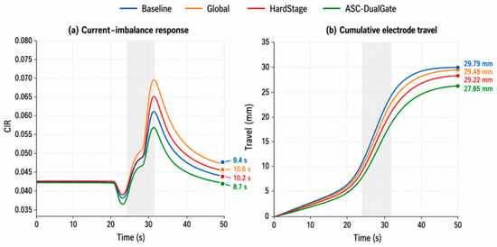
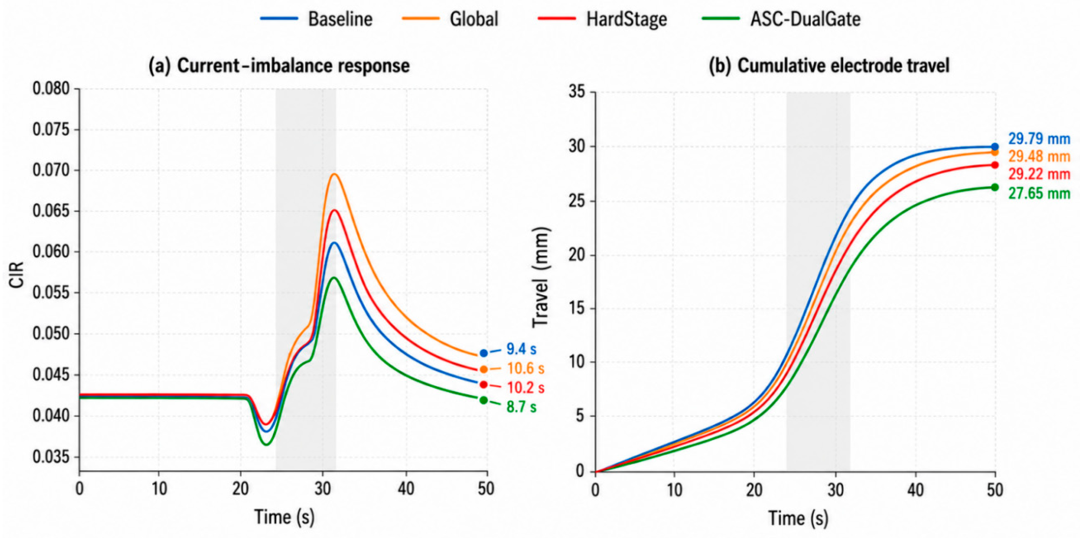
Table 12 reports CIR, VIR, normalized arc-power variance, cumulative electrode travel, recovery time, and cross-phase PPR across four simulated disturbances and 20 paired random seeds. Figure 11 is a summary-consistent illustration of the reported mean recovery times and mean terminal travel; it is not a raw trajectory from a selected simulation run.
Table 12.
Performance under four disturbance scenarios and 20 paired random seeds.
Figure 11.
Illustrative time-domain visualization consistent with the Table 12 across-scenario, 20-seed summary statistics: (a) current-imbalance response, where right-hand labels denote mean recovery time; and (b) cumulative electrode travel, where terminal labels denote mean travel. The curves are not raw trajectories from a single simulation run.
Figure 11 is a visualization fitted to the Table 12 summaries rather than an independently sampled transient. Its right-hand labels reproduce the mean recovery times (8.72 s for ASC-DualGate), while Table 12 provides the actual comparison over four disturbances and 20 paired seeds.
In Figure 11b, the terminal labels reproduce the Table 12 mean travel values; ASC-DualGate is 27.65 mm. The curves should be read only as summary-matched visual guides. The comparison is internal to the reduced actuator/controller model and is not a measurement of industrial electrode consumption or wear.
6.5. Summary
A simulation framework is constructed around disturbance propagation and closed-loop recovery in three-phase electrode regulation, and Baseline, Global, HardStage, and ASC-DualGate are compared.
Within the reduced platform, ASC-DualGate yields CIR = 0.0552, VIR = 0.0170, normalized power variance = 0.001248, travel = 27.65 mm, recovery = 8.72 s, and PPR = 0.3770. These are favorable relative comparisons for the tested simulated disturbances, not evidence of online industrial performance.
The simulation supports computational and control-loop plausibility under the stated model. Its remaining parameter mismatch, the omitted furnace physics, and the absence of hardware/plant actuation require prospective validation before deployment.
7. Conclusions
This study makes four scientific contributions. First, it formulates the three-phase matrices as closed-loop equivalent propagation maps and explicitly separates that object from open-loop physical sensitivity. Second, it introduces independent current/voltage risk gates with a mathematically bounded fallback family. Third, it treats statistical stages as optional candidate priors rather than unconditional switching commands or physical furnace stages. Fourth, it combines same-window replay, identification diagnostics, temporally separated leave-one-heat-out evaluation, and reduced closed-loop simulation so that complementary levels of evidence define the scope of the conclusions.
In same-window replay of four heats, ASC-DualGate reduces current-side ICR, voltage-side ICR, and J by 36.67%, 26.46%, and 30.98% relative to Global; event PPR and PER fall by 48.07% and 69.45%, relative to Raw. The ablation shows that residual-risk screening and safe fallback provide most of this aggregate improvement, while stage priors and separate side decisions add smaller, non-additive gains.
The temporally separated leave-one-heat-out replay provides a stricter assessment of transfer beyond the same-window structural analysis. Under this protocol, the performance advantage is reduced and varies across held-out heats, indicating sensitivity to short-term operating-condition changes. Accordingly, the 30.98% same-window result should be interpreted as evidence for the structural-selection mechanism within the investigated operating regime, while broader predictive transfer across time and heats requires further prospective evaluation.
The calibrated reduced simulator reproduces the broad electrical and actuator scales and provides known-structure diagnostics; however, it omits thermochemical dynamics and remains separate from the industrial replay. Its favorable comparative response supports feasibility of the supervisory logic, not online effectiveness on the 75 t furnace.
The demonstrated scope comprises archived data from four heats of one 75 t three-phase AC EAF under one incumbent regulator. Validation across other furnace capacities, transformer and short-network configurations, operating practices, and direct-current furnaces remains to be studied in future work. Prospective studies should acquire command signals for stronger instrumental-variable identification, calibrate gates on multiple furnaces, use independent train/validation/test cohorts and multi-objective Pareto tuning, and conduct safeguarded online trials to evaluate energy efficiency, production stability, electrode wear, and equipment life.
Author Contributions
Conceptualization, Z.R. and A.C.; methodology, Z.R. and A.C.; software, Z.R.; validation, Z.R., Q.C. and H.Z.; formal analysis, Z.R.; investigation, Q.C. and H.Z.; resources, A.C., Q.C. and H.Z.; data curation, Z.R. and H.Z.; writing—original draft preparation, Z.R.; writing—review and editing, A.C., Q.C., H.Z., F.L., J.L. and Z.W.; visualization, Z.R.; supervision, A.C.; project administration, A.C.; funding acquisition, A.C. All authors have read and agreed to the published version of the manuscript.
Funding
This work was supported by the Shaanxi Province Qinchuangyuan “Scientist + Engineer” Team Building Project (Grant No. 2023KXJ-247) and the Shandong Province Key Research and Development Program (Grant No. 2024TSGC0920), China.
Data Availability Statement
The industrial records are not publicly available because they contain commercially sensitive operating information from the partner plant. De-identified derived data may be requested from the corresponding author, subject to approval by the industrial data owner and applicable confidentiality restrictions. The numerical settings and analysis procedures required to interpret the reported results are provided in the manuscript.
Acknowledgments
The authors would like to thank the industrial partner for providing operational data and technical support during this study.
Conflicts of Interest
Author Haitao Zhang was employed by the company Xi’an Electric Furnace Research Institute Co., Ltd. The remaining authors declare that the research was conducted in the absence of any commercial or financial relationships that could be construed as a potential conflict of interest.
Nomenclature
| Symbol | Meaning | Unit |
| ASC-DualGate | Proposed risk-constrained dual-gated compensation method | — |
| GMM | Gaussian mixture model | — |
| PCA | Principal component analysis | — |
| BIC | Bayesian information criterion | — |
| ICR | Interphase coupling ratio | — |
| OER | Off-diagonal energy ratio | — |
| CIR | Current imbalance ratio | — |
| VIR | Voltage imbalance ratio | — |
| PPR | Peak propagation ratio | — |
| PER | Propagation energy ratio | — |
| MPR | Main-phase response ratio | — |
| t | Sampling time index | — |
| k | Sliding-window index | — |
| W | Sliding-window length | samples |
| S | Sliding step | samples |
| m | Propagation-stage index | — |
| M | Number of statistical propagation stages | — |
| L(t) | Equivalent electrode-position vector | mm |
| i(t) | Three-phase arc-current vector | kA |
| u(t) | Three-phase arc-voltage vector | V |
| ΔL(t) | Increment of equivalent electrode-position vector | mm |
| Δi(t) | Increment of three-phase arc-current vector | kA |
| Δu(t) | Increment of three-phase arc-voltage vector | V |
| Xk | Input matrix of electrode-position increments in window k | mm |
| YI,k | Output matrix of current increments in window k | kA |
| YU,k | Output matrix of voltage increments in window k | V |
| GI,k | Current-side local disturbance propagation matrix | kA/mm |
| GU,k | Voltage-side local disturbance propagation matrix | V/mm |
| GI,k | Normalized current-side propagation matrix | — |
| GU,k | Normalized voltage-side propagation matrix | — |
| Q | Structural decoupling matrix | — |
| Qg | Global decoupling matrix | — |
| Qm | Stage-aware decoupling matrix of stage m | — |
| Qb | Safe-fallback compensation candidate | — |
| Selected current-side decoupling matrix in window k | — | |
| Selected voltage-side decoupling matrix in window k | — | |
| HI,k | Compensated current-side propagation matrix | kA/mm |
| HU,k | Compensated voltage-side propagation matrix | V/mm |
| zk | Feature vector for propagation-stage identification | — |
| sk | Propagation-stage label of window k | — |
| PI,m | Current-side prototype matrix of stage m | kA/mm |
| PU,m | Voltage-side prototype matrix of stage m | V/mm |
| RI,k | Current-side residual structural risk | — |
| RU,k | Voltage-side residual structural risk | — |
| Jk | Overall structural risk in window k | — |
| J | Heat-averaged overall structural risk | — |
| λ | Ridge-regression regularization coefficient | — |
| κg, κs, κloc | Global, stage, and local structure-matching damping coefficients | — |
| τv | Viterbi stage-switching penalty coefficient | — |
| αI, βI, αU, βU | Weighting coefficients for overall structural-risk J | — |
| ‖ · ‖F | Frobenius norm | — |
| ε | Small positive constant for numerical stability | — |
| αA | Nominal ALID blending coefficient | — |
| qmax | ALID normalized compensation-deviation limit | — |
| μ | Safe-fallback blending coefficient | — |
References
- Hay, T.; Visuri, V.V.; Aula, M.; Echterhof, T. A review of mathematical process models for the electric arc furnace process. Steel Res. Int. 2021, 92, 2000395. [Google Scholar] [CrossRef] [Scilit]
- Abadi, M.M.; Tang, H.; Rashidi, M.M. A review of simulation and numerical modeling of electric arc furnace (EAF) and its processes. Heliyon 2024, 10, e32157. [Google Scholar] [CrossRef] [Scilit] [PubMed]
- Logar, V.; Dovžan, D.; Škrjanc, I. Modeling and validation of an electric arc furnace: Part 1, heat and mass transfer. ISIJ Int. 2012, 52, 402–412. [Google Scholar] [CrossRef] [Scilit]
- MacRosty, R.D.M.; Swartz, C.L.E. Dynamic modeling of an industrial electric arc furnace. Ind. Eng. Chem. Res. 2005, 44, 8067–8083. [Google Scholar] [CrossRef] [Scilit]
- Shyamal, S.; Swartz, C.L.E. Real-time energy management for electric arc furnace operation. J. Process Control 2019, 74, 50–62. [Google Scholar] [CrossRef] [Scilit]
- Olczykowski, Z. Modeling of voltage fluctuations generated by arc furnaces. Appl. Sci. 2021, 11, 3056. [Google Scholar] [CrossRef] [Scilit]
- Boulet, B.; Vaculik, V.; Wong, G. Control of non-ferrous electric arc furnaces. IEEE Can. Rev. 1997, 27, 4–8. [Google Scholar]
- Peens, M. Modelling and Control of an Electrode System for a Three-Phase Electric arc Furnace. Master’s Thesis, University of Pretoria, Pretoria, South Africa, 2006. [Google Scholar]
- Wang, Y.; Mao, Z.Z.; Tian, H.X.; Li, Y.; Yuan, P. Modeling of electrode system for three-phase electric arc furnace. J. Cent. South Univ. Technol. 2010, 17, 560–565. [Google Scholar] [CrossRef] [Scilit]
- Kozyra, J.; Lozynskyy, A.; Łukasik, Z.; Kuśmińska-Fijałkowska, A.; Kutsyk, A.; Kasha, L. Electric arc furnace electrode movement control system based on a fuzzy arc length identifier. Energies 2023, 16, 7281. [Google Scholar] [CrossRef] [Scilit]
- Feliu-Batlle, V.; Rivas-Perez, R.; Borges-Rivero, R.A.; Misa-Llorca, R. System identification for robust control of an electrode positioning system of an industrial electric arc melting furnace. Processes 2024, 12, 2509. [Google Scholar] [CrossRef] [Scilit]
- Ding, S.; Wang, Z.; Kong, W.; Yang, H.; Song, G. Electrode regulating system modeling in electrical smelting furnace using recurrent neural network with attention mechanism. Neurocomputing 2019, 359, 32–40. [Google Scholar] [CrossRef] [Scilit]
- Saboohi, Y.; Fathi, A.; Škrjanc, I.; Logar, V. Optimization of the electric arc furnace process. IEEE Trans. Ind. Electron 2019, 66, 8030–8039. [Google Scholar] [CrossRef] [Scilit]
- Jawahery, S.; Visuri, V.V.; Wasbø, S.O.; Hammervold, A.; Hyttinen, N.; Schlautmann, M. Thermophysical model for online optimization and control of the electric arc furnace. Metals 2021, 11, 1587. [Google Scholar] [CrossRef] [Scilit]
- Bekker, J.G.; Craig, I.K.; Pistorius, P.C. Model predictive control of an electric arc furnace off-gas process. Control Eng. Pract. 2000, 8, 445–455. [Google Scholar] [CrossRef] [Scilit]
- Tomažič, S.; Andonovski, G.; Škrjanc, I.; Logar, V. Data-driven modelling and optimization of energy consumption in electric arc furnaces. Metals 2022, 12, 816. [Google Scholar]
- Godoy-Rojas, D.F.; Leon-Medina, J.X.; Rueda, B.; Vargas, W.; Romero, J.; Pedraza, C.; Pozo, F.; Tibaduiza, D.A. Attention-based deep recurrent neural network to forecast the temperature behavior of an electric arc furnace side-wall. Sensors 2022, 22, 1418. [Google Scholar] [CrossRef] [Scilit] [PubMed]
- Dinh, M.T.; Prodan, I.; Lesage, O.; Mendes, E. Mixed-integer predictive control for a three-phase electric arc furnace producing silico manganese. In Proceedings of the 2024 European Control Conference, Stockholm, Sweden, 25–28 June 2024; pp. 1979–1984. [Google Scholar]
- Andonovski, G.; Tomažič, S. Comparison of data-based models for prediction and optimization of energy consumption in electric arc furnace (EAF). IFAC-PapersOnLine 2022, 55, 373–378. [Google Scholar] [CrossRef] [Scilit]
- Wei, D.; Craig, I.K.; Bauer, M. Multivariate economic performance assessment of an MPC controlled electric arc furnace. ISA Trans. 2007, 46, 429–436. [Google Scholar] [CrossRef] [Scilit] [PubMed]
- Paranchuk, Y.; Jancarczyk, D.; Falat, P. Study and analysis of dynamics and energy efficiency of arc steelmaking furnaces’ electric modes with a fuzzy control algorithm. Energies 2023, 16, 3451. [Google Scholar] [CrossRef] [Scilit]
- Kozyra, J.; Lozynskyy, A.; Łukasik, Z.; Kuśmińska-Fijałkowska, A.; Kutsyk, A.; Kasha, L. Increasing the level of autonomy of control of the electric arc furnace by weakening interphase interactions. Energies 2023, 16, 8114. [Google Scholar] [CrossRef] [Scilit]
- Ghiormez, L.; Panoiu, M.; Panoiu, C. Fuzzy logic controller for power control of an electric arc furnace. Mathematics 2024, 12, 3445. [Google Scholar] [CrossRef] [Scilit]
- Klimas, M.; Grabowski, D. Application of long short-term memory neural networks for electric arc furnace modeling. Appl. Soft Comput. 2023, 145, 110574. [Google Scholar] [CrossRef] [Scilit]
- Gok, G.; Salor, O.; Taplamacioglu, M.C. A new electric arc furnace model based on current waveform synthesis from distributions of DFT amplitudes and power system frequency. IEEE Trans. Ind. Appl. 2024, 60, 5872–5881. [Google Scholar] [CrossRef] [Scilit]
- Babaei, Z.; Samet, H.; Serikov, V.A. New power balance equations for modelling electric arc furnace. IET Gener. Transm. Distrib. 2025, 19, e70116. [Google Scholar] [CrossRef] [Scilit]
- Lozynskyy, A.; Kozyra, J.; Kutsyk, A.; Lukasik, Z.; Kusminska-Fijalkowska, A.; Kasha, L. Synthesis of an electric arc furnace electrode movement control system based on feedback linearization with PI or PIμ controllers. Energies 2025, 18, 4873. [Google Scholar] [CrossRef] [Scilit]
- Yu, F.; Mao, Z. Recursive identification for electric arc furnace-electrode regulator system. In Proceedings of the 36th Chinese Control Conference, Dalian, China, 26–28 July 2017; pp. 1989–1994. [Google Scholar]
- Babaei, Z.; Samet, H.; Jalil, M. An innovative approach considering active power and harmonics for modeling the electric arc furnace along with analyzing time-varying coefficients based on ARMA models. Int. J. Electr. Power Energy Syst. 2023, 153, 109377. [Google Scholar] [CrossRef] [Scilit]
- Hoerl, A.E.; Kennard, R.W. Ridge regression: Biased estimation for nonorthogonal problems. Technometrics 1970, 12, 55–67. [Google Scholar] [CrossRef] [Scilit]
- Landau, I.D.; Karimi, A. Recursive algorithms for identification in closed loop: A unified approach and evaluation. Automatica 1997, 33, 1499–1523. [Google Scholar] [CrossRef] [Scilit]
- Forssell, U.; Ljung, L. Closed-loop identification revisited. Automatica 1999, 35, 1215–1241. [Google Scholar] [CrossRef] [Scilit]
- Olczykowski, Z. Electric arc furnaces as a cause of current and voltage asymmetry. Energies 2021, 14, 5058. [Google Scholar] [CrossRef] [Scilit]
- Jolliffe, I.T. Principal Component Analysis, 2nd ed.; Springer: New York, NY, USA, 2002. [Google Scholar]
- Dempster, A.P.; Laird, N.M.; Rubin, D.B. Maximum likelihood from incomplete data via the EM algorithm. J. R Stat. Soc. Ser. B 1977, 39, 1–38. [Google Scholar] [CrossRef] [Scilit]
- Rabiner, L.R. A tutorial on hidden Markov models and selected applications in speech recognition. Proc. IEEE 1989, 77, 257–286. [Google Scholar] [CrossRef] [Scilit] [PubMed]
- Bristol, E.H. On a new measure of interaction for multivariable process control. IEEE Trans. Autom. Control 1966, 11, 133–134. [Google Scholar] [CrossRef] [Scilit]
- Hauksdóttir, A.S.; Gestsson, A.; Vésteinsson, A. Current control of a three-phase submerged arc ferrosilicon furnace. Control Eng. Pract. 2002, 10, 457–463. [Google Scholar] [CrossRef] [Scilit]
- Lu, J.; Huo, J.B.; Zhang, G.Y. Fuzzy decoupling controller on electrode regulator system of electric arc furnace. Trans. China Electrotech. Soc. 2015, 30, 27–33. [Google Scholar]
- He, J.; Liu, Y.; Yu, S.; Gui, W. Neural adaptive PSD decoupling controller and its application in three-phase electrode adjusting system of submerged arc furnace. J. Cent. South Univ. 2013, 20, 405–412. [Google Scholar] [CrossRef] [Scilit]
- Logar, V.; Dovzan, D.; Skrjanc, I. Mathematical modeling and experimental validation of an electric arc furnace. ISIJ Int. 2011, 51, 382–391. [Google Scholar] [CrossRef] [Scilit]
- Van den Hof, P.M.J. Closed-loop issues in system identification. Annu Rev. Control 1998, 22, 173–186. [Google Scholar] [CrossRef] [Scilit]

Disclaimer/Publisher’s Note: The statements, opinions and data contained in all publications are solely those of the individual author(s) and contributor(s) and not of MDPI and/or the editor(s). MDPI and/or the editor(s) disclaim responsibility for any injury to people or property resulting from any ideas, methods, instructions or products referred to in the content. |
© 2026 by the authors. Licensee MDPI, Basel, Switzerland. This article is an open access article distributed under the terms and conditions of the Creative Commons Attribution (CC BY) license.