Design of Multilateral Collaborative Adaptive Learning Controller for Nonlinear Dynamic System with External Disturbance and Backlash-like Hysteresis

Abstract

For lumped uncertainty caused by hysteresis saturated input, external disturbance and model uncertainty, traditional adaptive control accuracy depends on unilateral parameter learning and nonlinear approximation ability. To improve learning capability and trajectory-tracking performance under the considered uncertainty conditions, a multilateral collaborative adaptive learning mechanism and its corresponding controller are proposed. The initial value allocation of the multilateral uncertainty estimates are realized by means of arithmetic sequence or historical data points, and then the estimates are adjusted online based on the estimation errors of each side. The output result of multilateral weighted fusion is used as the compensation term of lumped uncertainty. An iterative learning framework based on compensation terms, dynamic self-learning approximation errors and the uncertainty estimates of each side is constructed to realize multilateral synchronous cyclic iterative learning, and a saturation transfer function is designed to ensure bounded continuous parameter changes. Controllers based on the linear extended state observer and the nonlinear extended state observer are taken as comparison schemes, the control characteristics of the proposed controller in manipulator systems are studied, and the effectiveness of the controller is verified.

1. Introduction

At present, industrial manipulators are widely used in assembly line production operations, improving the production and manufacturing capacity of automobiles, consumer electronics and other products. In order to improve the quality of products, the manipulator is required to have a fast response speed and high precision, and research on the manipulator has never stopped. Since it is difficult to establish an accurate dynamic model of the manipulator, the RBF neural network was used in references [1,2] to approximate the unmodeled part and unknown compound disturbance in the manipulator system, and a robust adaptive timing sliding mode controller and a finite-time trajectory tracking controller were designed, respectively. In reference [3], multi-layer neural networks were used to learn the uncertainties in the system and to offset the negative effects of complex nonlinear characteristics in the manipulator system in a feedforward manner. Some scholars have adopted extreme learning machines to overcome the challenges brought by model uncertainty, and reference [4] realized the fast timing trajectory tracking of the manipulator based on this method. In order to cope with the influence of model uncertainty and other nonlinearities in the flexible manipulator, an adaptive neural network and fuzzy logic system were used to design the controller in reference [5] and reference [6], respectively, to ensure the good action of the flexible manipulator. In reference [7], an adaptive model uncertainty estimator was used to design a model-free controller, which realized accurate trajectory tracking control. In reference [8], a model-free digital adaptive control algorithm was designed to effectively overcome the challenges brought by problems such as model uncertainty. Considering the influence of unmodeled dynamics and external disturbance, an adaptive sliding mode disturbance observer was proposed in reference [9] to realize active disturbance rejection control. By designing an extended state observer, the uncertainty of the joint stiffness of the manipulator described in reference [10] was estimated and eliminated to ensure the control performance of the joint state.

In order to solve the problems of uncertain parameters and external disturbance in the manipulator system, an adaptive iterative learning control algorithm based on disturbance estimation was designed in reference [11] to effectively overcome the influence of disturbance. By using a disturbance observer, reference [12] compensated for unknown external disturbance to ensure the safety of physical human–computer interaction. In references [13,14], adaptive neural networks were used to offset the negative effects of external perturbation, and a predefined time tracking controller and a neural network adaptive controller were designed, respectively. In reference [15], a neural network disturbance observer was combined with a dynamic surface controller. The observer was used to compensate the uncertainty and external disturbance of the manipulator online, and an adaptive dynamic surface controller of the electric manipulator system was designed. In reference [16], three disturbance estimators were proposed to approximate the upper bound of external disturbance, and a composite adaptive boundary iterative learning controller was designed. In order to solve this kind of problem in the manipulator, a new disturbance observer was designed in reference [17], which compensated the total disturbance in the system. In a trajectory tracking control scenario for an underwater manipulator, reference [18] designed an adaptive sliding mode tracking controller based on a nonlinear disturbance observer to overcome the influence of underwater major disturbance and to improve the stability and robustness of the manipulator. Reference [19] proposed an adaptive impedance control method based on a nominal model to solve the problems of unmodeled dynamics and external disturbance. For the study of unmanned aerial systems, reference [20] introduced an adaptive sliding mode disturbance observer with nested adaptive structure, which successfully compensated the influence of external disturbance and state uncertainty.

Hysteresis characteristics are widely present in mechanical transmission systems, posing a challenge to the control of industrial manipulators. Reference [21] considered the gap hysteresis and frictional nonlinearity problems in a three-degrees-of-freedom manipulator, adopted radial basis neural network to approach the unmodeled dynamics, and hyperbolic tangent neural network to approach the hysteresis characteristics, solved the relevant problems, and realized the trajectory tracking of the three-degree-of-freedom manipulator. Similarly, reference [22] used a radial basis neural network to approach unmodeled dynamics and to overcome the influence of hysteretic inputs by approximating intermediate variables. In reference [23], a neural network adaptive controller based on an immune algorithm was designed to solve problems such as hysteretic nonlinearity and model uncertainty in multi-joint manipulators. Through the application of inversion technology and the adaptive neural network method, a state feedback controller was designed in reference [24] to solve problems such as hysteresis in the system. Based on the finite time control theory and the sliding mode control method, a robust model-free controller was designed in reference [25] to ensure good trajectory tracking of the manipulator. Considering various nonlinearities such as hysteresis in the system as lumped nonlinearities, RBF neural networks were used in reference [26] to approximate and compensate their effects. To solve the same kind of problems in the manipulator, references [27,28] designed a fast terminal sliding mode controller combined with the delay estimation theory to ensure the robustness of the closed-loop system. Reference [29] studied a manipulator with unknown gear clearance and proposed an adaptive robust control method to solve related problems. Considering the hysteresis characteristics and flexible vibration problems in a rigid flexible coupled manipulator system, a robust adaptive iterative learning output feedback controller was designed in reference [30] combined with a neural network state observer to achieve good trajectory tracking of the manipulator.

It is a common control method to consider the many kinds of nonlinearity and external disturbances in a manipulator system as lumped uncertainties, which can be compensated online by designing approximators or observers. References [31,32,33] studied different manipulator systems, all of which used neural networks to approach lumped uncertainties online to improve the control effect. Facing the problem of position tracking control of a cable-driven manipulator, references [34,35,36] used the theory of time delay estimation to design controllers that are effective for a variety of nonlinearities. In order to meet the needs of human–computer interaction, reference [37] compensated lumped uncertainty by designing an adaptive update rate to achieve accurate control of the manipulator. In reference [38], a robust controller was designed for a rigid link electric drive manipulator system, which effectively overcame the influence of lumped uncertainty. In reference [39], Chebyshev polynomials were used to estimate lumped uncertainty, which reduced the computational complexity to some extent. For the study of an electrically driven manipulator [40,41], Bernstein polynomials were used to approximate lumped uncertainties and an effective control scheme was designed. In order to solve this problem, references [42,43] designed an adaptive sliding mode disturbance observer and an adaptive super twisting observer, respectively, to compensate lumped uncertainties in the system. An extended state observer can also compensate the total disturbance of a system, which was verified in references [44,45,46].

Although various existing controllers can ensure good trajectory-tracking performance of manipulator systems, several challenges remain when dealing with multiple complex nonlinear behaviors:

• Designing a controller with good robustness is still a difficult problem. Many kinds of nonlinearities exist in nonlinear dynamic systems, which are usually sensitive and burden the tracking accuracy of the system, so it is necessary to improve the robustness of the controller.
• The learning adaptability of nonlinear dynamic control algorithms needs to be further improved. It is usually difficult to obtain an accurate model of a nonlinear dynamic system. In a control process, it is beneficial to adjust the parameters in real time to learn to adapt to unknown changes.

To meet the needs of intelligent manufacturing and high-precision machining, this paper proposes a model reference multilateral learning adaptive control strategy. The proposed model reference multilateral learning adaptive controller is designed to compensate for combined hysteresis, input saturation, and model uncertainty, and it was evaluated under the operating conditions considered in this study. Our specific contributions are as follows:

• A multilateral learning adaptive mechanism is proposed and designed, and an iterative learning framework based on lumped uncertainty compensation, dynamic self-learning approximation error and uncertainty estimates on each side is constructed to realize multilateral synchronous cyclic iterative learning. The control law is designed by using the multilateral learning output as the compensation term considering the lumped uncertainty of various nonlinear characteristics in a nonlinear dynamic system. A second-order linear filter is used to obtain the differential signal to update the system state and reduce the computational complexity.
• The initial value allocation strategy of the multilateral learning adaptive mechanism was studied. Based on the available prior knowledge of the lumped uncertainty, two cases were considered: partial known data distribution characteristics and unknown data distribution characteristics. For the case where the distribution characteristics of the partial data were known, the multilateral uncertainty estimates were designed as the equivalent loci of the data. For unknown cases, the initial value was assigned by evenly distributing the values at equal intervals.
• The adaptive update rate of each side uncertainty was designed based on the multilateral uncertainty estimation error, and the adaptive update rate of the multilateral weight was designed based on the multilateral uncertainty value and the fitting error of the control closed loop to the lumped uncertainty. In order to avoid the chattering phenomenon caused by the excessive change rate of multilateral weight parameters, the saturation conversion function was designed to constrain change rate within the specified range, which makes the signal change smoother and bounded.

The rest of the paper is arranged as follows: In Section 2, the complex nonlinear problems that need to be solved in the nonlinear dynamic system are presented. In Section 3, a model reference multilateral learning adaptive controller is proposed and designed. An initial value allocation strategy and adaptive update rate are designed for multilateral uncertainty estimates and multilateral weights. Section 4 provides a Lyapunov-based stability analysis of the control system. In Section 5, controllers based on a linear extended state observer and a nonlinear extended state observer are compared to verify the effectiveness of the proposed controller. The conclusion is given in Section 6.

2. Problem Formulation

Consider the following n-order nonlinear dynamical system:

$$\left\{\begin{array}{c}{\dot{x}}_1=x_2\hfill \\ {\dot{x}}_2=M^{-1}\left(q\right)\left(w\left(\tau \right)+{\tau }_d-C\left(q,\dot{q}\right)\dot{q}-G\left(q\right)\right)\hfill \end{array}\right.$$

(1)

where $q\in {\mathbb{R}}^n$ represents the position vector, $\dot{q}\in {\mathbb{R}}^n$ represents the velocity vector, and $\ddot{q}\in {\mathbb{R}}^n$ represents the acceleration vector. $M\left(q\right)\in {\mathbb{R}}^{n\times n}$ is the inertial matrix, $C(q,\dot{q})\in {\mathbb{R}}^{n\times n}$ is the Coriolis force and centrifugal force matrix, and $G\left(q\right)\in {\mathbb{R}}^n$ is the gravity vector. The right side of the equal sign represents the control input of the nonlinear dynamical system, $\tau \in {\mathbb{R}}^n$ represents the control torque, $w\left(\tau \right)\in {\mathbb{R}}^n$ represents the backlash-like hysteresis characteristic, and ${\tau }_d\in {\mathbb{R}}^n$ represents the external disturbance. There is a definition of the state variables: $x_1=q$, $x_2=\dot{q}$. And $M^{-1}\left(q\right)$ is the inverse of $M\left(q\right)$.

Assumption 1. 

An accurate model of the inertia matrix $M\left(q\right)$ is difficult to establish, and its approximate nominal value is known, denoted by $M_0\left(q\right)$. The nominal matrix satisfies the condition of invertibility, and the inverse matrix is expressed as $M_0^{-1}\left(q\right)$.

Assumption 2. 

Matrices $C(q,\dot{q})$ and $G\left(q\right)$ are completely unknown and need to be considered as uncertain parts of the model. The external disturbance ${\tau }_d$ is bounded, and there exists a positive constant ${\overline{\tau }}_d$ that satisfies $\parallel {\tau }_d\parallel \le {\overline{\tau }}_d$, where $\parallel ·\parallel$ represents the norm of the vector.

Consider tracking the state trajectory of a linear reference system whose state is $x_r={\left[\begin{array}{c}{x}_{r1},x_{r2}\end{array}\right]}^T\in {\mathbb{R}}^{2n}$, and the state space model is as follows:

$$\left\{\begin{array}{c}{\dot{x}}_{r1}={\dot{x}}_{r2}\hfill \\ {\dot{x}}_{r2}=-{\lambda }_1{x}_{r1}-{\lambda }_2{x}_{r2}+u_r\hfill \end{array}\right.$$

(2)

where ${\lambda }_1,{\lambda }_2>0$, are positive constants, and where $u_r\in {\mathbb{R}}^n$ is the control signal of the reference system to ensure that the state of the reference system is tracked on the desired trajectory; usually a tracking error feedback control rate is selected.

Assuming that the expected joint trajectory is represented as $r\in {\mathbb{R}}^n$ and that the expected joint velocity trajectory is $\dot{r}\in {\mathbb{R}}^n$, the tracking error of the linear reference system is calculated as

$$e_{r1}=r-x_{r1}$$

(3)

$$e_{r2}=\dot{r}-x_{r2}$$

(4)

Symbols $e_{r1}\in {\mathbb{R}}^n$ and $e_{r2}\in {\mathbb{R}}^n$ are the joint angle tracking error and joint angular velocity tracking error of the reference system, respectively. The design error feedback control rate is

$$u_r=k_{r1}{e}_{r1}+k_{r2}{e}_{r2}$$

(5)

where $k_{r1},k_{r2}>0$ are the control gain.

Property 1 

([47]). The backlash-like hysteresis model is represented as

$${\displaystyle \frac{dw}{dt}}=\alpha \left|{\displaystyle \frac{d\tau }{dt}}\right|(c\tau -w)+B{\displaystyle \frac{d\tau }{dt}}$$

(6)

The model parameters $\alpha ,c,B$, which are three different constants, need to satisfy $c>0$ and $c>B$. Equation (6) has the solution of the differential equation, as shown in Equations (7) and (8):

$$w\left(\tau \right)=c\tau +R\left(\tau \right)$$

(7)

$$\begin{array}{cc}\hfill R\left(\tau \right)& =\left(w_0-c{\tau }_0\right)e^{-\alpha \left(\tau -{\tau }_0\right)\mathrm{sgn}\left(\dot{\tau }\right)}\hfill \\ \hfill & +e^{-\alpha \tau \mathrm{sgn}\left(\dot{\tau }\right)}{\int }_{{\tau }_0}^{\tau }(B-c)e^{\alpha \xi \mathrm{sgn}\left(\dot{\tau }\right)}d\xi \hfill \end{array}$$

(8)

where $w_0$ and ${\tau }_0$ represent the initial values of the corresponding variables. $R\left(\tau \right)$ consists of complex nonlinear functions, which are difficult to calculate directly, but the term is bounded and there is a positive constant $\overline{R}$ that satisfies $∥R\left(\tau \right)∥\le \overline{R}$.

Assumption 3. 

Parameters $\alpha ,c,B$ in the hysteretic differential equation model are known and can directly participate in updating the system state.

Remark 1. 

The nonlinear dynamic system is affected by the model uncertainty, external disturbance and hysteresis characteristics, and the problem of saturated input nonlinearity will be introduced in the design of the controller in Section 3. The system is a complex nonlinear system. The objective of the control is to make the joint angle and joint angular velocity of each joint of the nonlinear dynamic system track the state trajectory of the linear reference system.

3. Controller Design

3.1. Controller Based on State Error Feedback and Model Compensation

Equation (7) is substituted into Equation (1) of the nonlinear dynamic system model, then

$$\left\{\begin{array}{c}{\dot{x}}_1=x_2\hfill \\ {\dot{x}}_2=M^{-1}\left(q\right)(c\tau +R\left(\tau \right)+{\tau }_d-C(q,\dot{q})\dot{q}-G\left(q\right))\hfill \end{array}\right.$$

(9)

It is not difficult to see that the parentheses to the right of the equal sign are computable only for a linear term about $\tau$. As mentioned in Assumption 1, we know $M_0$, the nominal value of the inertia matrix. Thus, Equation (9) can be transformed into

$$\left\{\begin{array}{cc}\hfill {\dot{x}}_1=& x_2\hfill \\ \hfill {\dot{x}}_2=& M_0^{-1}c\tau +\left(M^{-1}-M_0^{-1}\right)c\tau \hfill \\ \hfill & +M^{-1}\left(R\left(\tau \right)+{\tau }_d-C\dot{q}-G\right)\hfill \end{array}\right.$$

(10)

The uncertain part of the model, the external disturbance, the nonlinear term of hysteresis characteristics and the nominal unmodeled torque term in the system are considered as lumped uncertainties, denoted as f, yielding

$$f=\left(M^{-1}-M_0^{-1}\right)c\tau +M^{-1}\left(R\left(\tau \right)+{\tau }_d-C\dot{q}-G\right)$$

(11)

At this point, the nonlinear dynamic system can be simplified as

$$\left\{\begin{array}{c}{\dot{x}}_1=x_2\hfill \\ {\dot{x}}_2=M_0^{-1}c\tau +f\hfill \end{array}\right.$$

(12)

It is necessary to design a lumped uncertainty estimator to compensate for this item when controlling the manipulator to achieve state trajectory tracking, so as to minimize the adverse effects of complex nonlinearity on the system.

Define the tracking error of the manipulator as

$$e_1=x_{r1}-x_1$$

(13)

$$e_2=x_{r2}-x_2$$

(14)

Assumption 4. 

Both the reference state $x_r$ and the system state x of the manipulator are measurable, and the measured value can be directly involved in the calculation of the formula without considering the measurement noise.

Assumption 5. 

There exists an estimator that can directly compensate for the effects of a variety of complex nonlinearities, and $\widehat{f}$ is an estimate of lumped uncertainty.

Design the controller as

$$\tau =(-{\lambda }_1{x}_1-{\lambda }_2{x}_2+u_r-\widehat{f}+k_1{e}_1+k_2{e}_2)/\left(M_0^{-1}c\right)$$

(15)

where $k_1,k_2>0$ are the control gain.

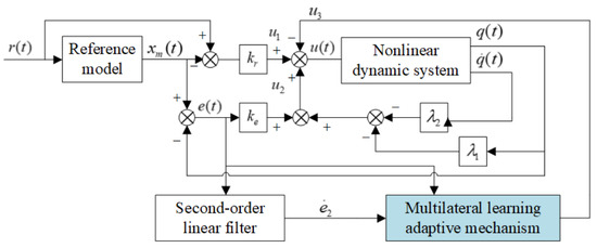
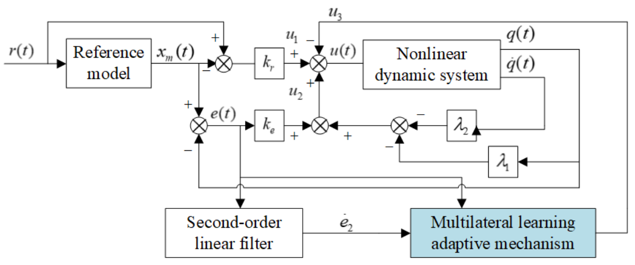
There are two control gains, $k_r$ and $k_e$, in Figure 1, denoted as $k_r={\left[\begin{array}{c}{k}_{r1},k_{r2}\end{array}\right]}^T$ and $k_e={\left[\begin{array}{c}{k}_1,k_2\end{array}\right]}^T$, respectively. The input of the reference model is $r\left(t\right)$ and the state is $x_m\left(t\right)$, and the error between the input and the state is calculated as the control action $u_r$, which is $u_1$ in the figure. The deviation calculated between the reference state and the state $q\left(t\right)$ of the multi-input and multi-output nonlinear dynamic system is used to design the error feedback control rate. The state $q\left(t\right)$ and $\dot{q}\left(t\right)$ of the system get the state feedback control rate through different combinations of amplification gain, and the two together constitute the control action $u_2$. In order to overcome the adverse effects of various complex nonlinear characteristics on the nonlinear dynamic system, a second-order linear filter is used to filter the error signal $e\left(t\right)$ and obtain the error differential, and it is incorporated in the design of a multilateral learning adaptive mechanism to form a control effect $u_3$. The model of the second-order linear filter is provided in the section on the multilateral learning adaptive update rate for parameters. In fact, the control action $u_3$ is the estimation of the lumped uncertainty

$$u_3=\widehat{f}$$

(16)

$$\begin{array}{cc}\hfill \tau & =u/\left(M_0^{-1}c\right)\hfill \\ & =\left(u_1+u_2+u_3\right)/\left(M_0^{-1}c\right)\hfill \end{array}$$

(17)

Figure 1. Control structure of nonlinear dynamic system based on state error feedback and model compensation.

Remark 2. 

The control rate of the linear reference system is introduced into the controller of the nonlinear dynamic system. This part plays a positive role in the dynamic expression of analytical error, which can directly compensate the control behavior of the reference system, avoid the additional adverse effects on the nonlinear dynamic system, and ensure the effectiveness of the controller.

Since the actuators of the nonlinear dynamic system are usually limited, a saturation nonlinear effect is generated, so that $\overline{\tau }$ represents the upper bound of the control torque, which is a column vector, where the elements correspond to the saturation amplitude of the actuators. At this point, $\tau$ is updated to

$$\tau =\left\{\begin{array}{c}\overline{\tau },\tau \ge \overline{\tau }\hfill \\ \tau ,-\overline{\tau }<\tau <\overline{\tau }\hfill \\ -\overline{\tau },\tau \le -\overline{\tau }\hfill \end{array}\right.$$

(18)

Remark 3. 

Control signal constraints exist widely in practical nonlinear control objects, which is an unavoidable nonlinear characteristic in the control process. Usually, choosing the appropriate control gain parameter can reduce the frequency of the control signal reaching the amplitude; in addition, an effective control structure will also have a positive effect.

3.2. Multilateral Initial Value Assignment Strategy for Lumped Uncertainty

Prior knowledge of the lumped uncertain part is usually non-existent or incomplete. Adopting an initial value selected subjectively in the design of the controller often brings a long transient adjustment stage, and the overall tracking error is also related to the selection of the initial value. Considering the correlation between the selection of initial values and the cumulative error of the process, a set of different initial values can be determined according to the characteristics of the continuous time data distribution of the lumped uncertainty, and the final estimate can be obtained by multilateral weights fusion. Initial value selection can be divided into two cases: (1) lumped uncertainty is completely unknown, which is a general case and covers a wide range; (2) the distribution characteristics of the lumped uncertainty are known, which is a special case and holds in a specific environment. For the first case, assuming that the lumped uncertainty follows the data characteristics of uniform distribution, such an initial set of values is obtained based on the set number of edges and the predetermined upper and lower bound arithmetic difference. For the second case, the historical data is restored based on the data distribution characteristics, and then a set of initial values is obtained by determining the bisection points according to the set number of edges.

In general, the inherent law of lumped uncertainty is elusive, and the first case can be used to obtain the initial value of the set edge number in most cases. Only the first case is considered below, and the initial value assignment is completed based on the assumed uniform distribution. Suppose that to select m edges each edge starts with an initial estimate of lumped uncertainty and completes the estimate update under mathematical laws. Define the estimated value of each side as ${\widehat{f}}_i\left(t\right)(i=1,2,\cdots ,m)$ and the estimated initial value as ${\widehat{f}}_i\left(0\right)$. Then the estimated error ${\tilde{f}}_i$ for each side is

$${\tilde{f}}_i=f-{\widehat{f}}_i$$

(19)

If the true lumped uncertainty is f and the estimated value of the lumped uncertainty in the control closed loop is $\widehat{f}$ then the estimated error $\tilde{f}$ of the control closed loop is

$$\tilde{f}=f-\widehat{f}$$

(20)

Remark 4. 

As will be seen in the following sections, the value of $\tilde{f}$ can be calculated based on the error dynamic relationship, and $\widehat{f}$ can be obtained by merging the multilateral weights with the multilateral uncertainty estimates in a certain way, so that f can ideally be calculated accurately. In fact, due to the existence of noise and the non-stationarity of data, there may be a small range of errors between the calculated lumped uncertainty and the true value; $f_{ref}$ may be used to represent the calculated lumped uncertainty:

$$f_{ref}=\widehat{f}+\tilde{f}$$

(21)

Equations (19) and (20) can be written in computable form:

$${\tilde{f}}_i=f_{ref}-{\widehat{f}}_i$$

(22)

$$\tilde{f}=f_{ref}-\widehat{f}$$

(23)

Remark 5. 

Since the nonlinear dynamic system may have multiple joints, a quantity representing uncertainty will be involved in the status update corresponding to each joint. Symbols $f,\widehat{f},\tilde{f},f_i,{\widehat{f}}_i,{\tilde{f}}_i,f_{ref}$ are vectors about lumped uncertainty, with different physical meanings. The length of the vector is the number of joints of the manipulator.

Suppose that the predetermined upper bound of the lumped uncertainty is $l_b\in {\mathbb{R}}^n$, the lower bound is $l_a\in {\mathbb{R}}^n$, and the element at a certain position in vector $l_a$ must always be smaller than the element at the same position in $l_b$. The length of a predetermined range is $s_1=l_b-l_a\in {\mathbb{R}}^n$, and the elements are positive. When the upper and lower bounds are symmetric about the origin, we have $l_a=-l_b$. The initial estimate of the lumped uncertainty of the m edges is calculated as

$$\begin{array}{cc}\hfill {\widehat{f}}_i\left(0\right)& =l_a+{\displaystyle \frac{l_b-l_a}{m-1}}(i-1)\hfill \\ \hfill & =l_a+{\displaystyle \frac{s_1}{m-1}}(i-1)\hfill \end{array}$$

(24)

The weight of each edge is defined as $w_i\left(t\right)(i=1,2,\cdots ,m)\in {\mathbb{R}}^n$, which is the weight coefficient vector corresponding to the i-th edge, and the initial weight is $w_i\left(0\right)$. In order to ensure that the lumped uncertainty estimates of different initial values contribute the same degree to the estimates of the control closed loop at the initial time, the weights are adjusted adaptively based on their estimation errors, and the initial weights of different edges are set to be equal at the initial time. Accordingly, only the initial weights are normalized to provide equal contributions from different edges at the initial instant, as given in (25). During online adaptation, the weights are allowed to deviate from the normalized condition according to their estimation performance:

$$w_i\left(0\right)={\displaystyle \frac{1}{m}}$$

(25)

Considering the linear fusion of the estimated value of m edges, on the one hand, the structure of the introduced control loop is relatively simple; on the other hand, linear fusion is beneficial to the design of the adaptive rate of multilateral weight parameters:

$$\widehat{f}={\displaystyle \sum _{i=1}^m}diag\left(w_i\right){\widehat{f}}_i$$

(26)

Remark 6. 

Even if the reference value $f_{ref}$ of the lumped uncertainty is not exactly consistent with the true value f of the uncertainty in the actual situation, the use of $f_{ref}$ in the calculation will not destroy the inherent characteristics of the system data. The two have the same law of change, and at any time in the allowed small error range they tend to be consistent. In addition, the estimate of the lumped uncertainty does not need to be fully accurate for ${\widehat{f}}_i$, allowing a certain degree of error. After the fusion of m estimates by multilateral learning strategy, the error limit of the estimation range is tightened, and a more accurate estimate of the lumped uncertainty is obtained.

3.3. Parameter Multilateral Learning Adaptive Update Rate

Take the derivative of Equations (13) and (14) and substitute the Equations (2) and (12); then

$$\left\{\begin{array}{c}{\dot{e}}_1=e_2\hfill \\ {\dot{e}}_2=-{\lambda }_1{x}_{r1}-{\lambda }_2{x}_{r2}+u_r-M_0^{-1}c\tau -f\hfill \end{array}\right.$$

(27)

Further, substitute Equation (15) into Equation (27) to get

$$\left\{\begin{array}{c}{\dot{e}}_1=e_2\hfill \\ {\dot{e}}_2=-({\lambda }_1+k_1)e_1-({\lambda }_2+k_2)e_2-\tilde{f}\hfill \end{array}\right.$$

(28)

It is not difficult to see from Equation (28) that the calculation form of $\tilde{f}$ is

$$\tilde{f}=-({\lambda }_1+k_1)e_1-({\lambda }_2+k_2)e_2-{\dot{e}}_2$$

(29)

A new problem is that the value of ${\dot{e}}_2$ cannot be determined, and in fact it is difficult to calculate analytically. Consider using a second-order linear filter to get its value. Since the manipulator has n degrees of freedom, such n filters are required. The model of the filter is

$$\left\{\begin{array}{c}{\dot{\widehat{m}}}_1={\widehat{m}}_2\hfill \\ {\dot{\widehat{m}}}_2=-2{\zeta }_f{\omega }_f{\widehat{m}}_2+{\omega }_f^2\left(m_1-{\widehat{m}}_1\right)\hfill \end{array}\right.$$

(30)

where

$$\left\{\begin{array}{c}{\widehat{m}}_1\left(0\right)=m_1\left(0\right)\hfill \\ {\widehat{m}}_2\left(0\right)=0\hfill \end{array}\right.$$

(31)

The filter parameters are ${\omega }_f$ and ${\zeta }_f$, representing the natural frequency and damping ratio, respectively; ${\widehat{m}}_1$ is the estimated form of $m_1$; and ${\widehat{m}}_2$ is the estimated form of ${\dot{m}}_1$. In the calculation of the uncertainty estimation error, $m_1=e_2$, and ${\widehat{m}}_2$ is used as the estimate of ${\dot{e}}_2$, denoted by ${\widehat{\dot{e}}}_2$. Define the filter estimation error as

$$d_f={\dot{e}}_2-{\widehat{\dot{e}}}_2.$$

(32)

For ${\omega }_f>0$ and ${\zeta }_f>0$, the homogeneous dynamics of the second-order filter are asymptotically stable. However, the stability of the filter alone does not directly establish the boundedness of the derivative estimation error $d_f$, because the filter input is coupled with the tracking-error dynamics. Therefore, the boundedness of $d_f$ is not assumed in advance. Instead, its ultimate bound is derived jointly with the tracking-error and uncertainty-estimator states under the sufficient conditions specified in Section 4. The term $d_f$ represents the difference between the actual error derivative and the filter output, including the influence of the filter-induced phase lag.

The symbol ${\Gamma }_e=diag\left(\left[{\gamma }_{e1},{\gamma }_{e2},\cdots ,{\gamma }_{en}\right]\right)\in {\mathbb{R}}^{n\times n}$ is defined as the learning rate matrix of the multilateral uncertainty estimate, where $diag(·)$ represents turning the input vector into a diagonal matrix, and ${\gamma }_{ej}\left(j=1,2,\cdots ,n\right)$ is the uncertainty learning rate of the corresponding joint of the manipulator. In special cases, the selected learning rate gain is the same—that is, ${\gamma }_{ej}={\gamma }_{ek}\left(j\ne k\right)$, in which only one parameter can be adjusted to achieve multiple joint learning rate configurations. The renewal rate of the design multilateral uncertainty is

$${\dot{\widehat{f}}}_i={\Gamma }_e({\tilde{f}}_i+d_f)$$

(33)

For the unsaturated control-input regime, the above estimator update is an equivalent error representation. In practical implementation, the term ${\tilde{f}}_i+d_f$ is evaluated as ${\tilde{f}}_c+\widehat{f}-{\widehat{f}}_i$, where

$${\tilde{f}}_c=-({\lambda }_1+k_1)e_1-({\lambda }_2+k_2)e_2-{\widehat{\dot{e}}}_2.$$

(34)

Here, ${\tilde{f}}_c$ denotes the computable uncertainty estimation-error signal obtained using the filtered derivative. For the unsaturated control-input regime, it satisfies ${\tilde{f}}_c=\tilde{f}+d_f$.

The symbol $\Gamma =diag\left(\left[{\gamma }_1,{\gamma }_2,\cdots ,{\gamma }_n\right]\right)\in {\mathbb{R}}^{n\times n}$ is defined as the learning rate matrix of multilateral weights, where ${\gamma }_j(j=1,2,\cdots ,n)$ is the parameter learning rate of the corresponding joint of the manipulator. The adaptive update rate of the multilateral weight parameter is designed as

$${\dot{w}}_i=\Gamma \mathrm{diag}\left({\widehat{f}}_i\right){\tilde{f}}_c$$

(35)

It is worth noting that too-fast parameter changes will bring high-frequency oscillations, which may deteriorate the control quality of the system, so it is necessary to use certain methods to avoid too-fast parameter changes and to ensure certain continuity. Consider designing a saturation conversion function to accomplish this task, using $l_d$ to represent the upper bound of the function, with 

$$sat\left(z,l_d\right)={\displaystyle \frac{l_d}{1+e^{-z}}}-{\displaystyle \frac{l_d}{1+e^z}}$$

(36)

where z is the input to the saturation conversion function. To constrain both the weight update rate and magnitude, the adaptive law in Equation (35) is modified as

$${\dot{w}}_i={\mathrm{Proj}}_{{\Omega }_w}\left[w_i,sat\left(\Gamma \mathrm{diag}\left({\widehat{f}}_i\right){\tilde{f}}_c,l_d\right)\right]$$

(37)

where ${\mathrm{Proj}}_{{\Omega }_w}(·)$ denotes the projection operator and

$${\Omega }_w=\left\{w_i\in {\mathbb{R}}^n:{\parallel w_i\parallel }_{\infty }\le \overline{w}\right\},$$

(38)

For the revised theoretical formulation, the prescribed projection bound is selected as $\overline{w}=1$. With $m=7$ and $w_i\left(0\right)=1/7$, the initial weights satisfy $\parallel w_i{\left(0\right)\parallel }_{\infty }<\overline{w}$.

Let $v_i=\mathrm{sat}\left(\Gamma \mathrm{diag}\left({\widehat{f}}_i\right){\tilde{f}}_c,l_d\right)$. The projection operator is defined componentwise as

$${\left[{\mathrm{Proj}}_{{\Omega }_w}(w_i,v_i)\right]}_j=\left\{\begin{array}{cc}0,\hfill & w_{i,j}=\overline{w},v_{i,j}>0,\hfill \\ 0,\hfill & w_{i,j}=-\overline{w},v_{i,j}<0,\hfill \\ v_{i,j},\hfill & \mathrm{otherwise}.\hfill \end{array}\right.$$

The projection operator suppresses the outward-pointing updates at the prescribed boundaries and leaves the other updates unchanged. Consequently, if $w_i\left(0\right)\in {\Omega }_w$ then $w_i\left(t\right)\in {\Omega }_w$ for all $t\ge 0$.

The corresponding stability result is subject to the common quadratic-stability condition in (82).

Remark 7. 

Parameter $l_d$ of the saturation conversion function can be either a scalar or a vector. In general, if the parameter z is a scalar then $l_d$ is also a scalar; if the parameter z is a vector then $l_d$ is also a vector, and elements at the same position correspond to each other to achieve a single limiting of elements at different positions. In addition, to reduce the number of adjustable parameters, if the input is a vector then the elements in $l_d$ can be set to be equal, which is equivalent to the passed $l_d$ being a scalar. However, this simplified scheme is not conducive to the control of a multi-input, multi-output system, and multilateral weight parameters with different degrees of freedom have different requirements for saturation values.

It should be emphasized that the saturation conversion function limits the update rate of the multilateral weights, whereas the projection operator guarantees the boundedness of the weights themselves. These two mechanisms therefore play different roles. The normalization in (25) is imposed only on the initial weights and is not required to be maintained during online adaptation.

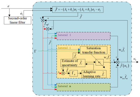
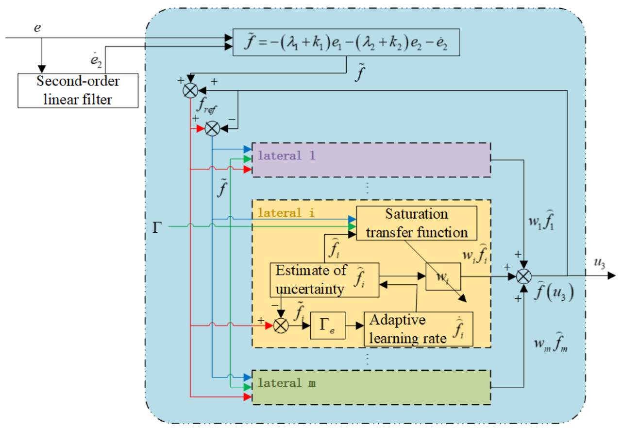
Figure 2 illustrates the multilateral learning adaptive mechanism, and the multilateral learning result $\widehat{f}$ is the third control action $u_3$ of the controller. Error signal e is passed through the second-order linear filter to obtain the differential signal of error, and the estimation error of the lumped uncertainty of the control closed loop is calculated by Equation (29). The error is added to the estimate of the lumped uncertainty of the control closed loop to obtain the reference value of the uncertainty, and the deviation of the selected m edges relative to the reference value is used to update the uncertainty estimates from adaptation. The linear fusion of multiple estimates and corresponding multilateral weights forms the estimate $\widehat{f}$ of the lumped uncertainty of the control closed loop. The computable error ${\tilde{f}}_c$ and the individual estimates ${\widehat{f}}_i$ are used to update the multilateral weights through the saturation conversion function and projection operator. The outputs of m edges are linearly fused together to achieve a final estimate of the lumped uncertainty:

Figure 2. Multilateral collaborative adaptive learning mechanism.

The implementation procedure of the proposed controller is summarized in Algorithm 1.

Algorithm 1 Model reference multilateral learning adaptive controller for nonlinear dynamical systems

Input: desired trajectory $r_i,{\dot{r}}_i,{\ddot{r}}_i$, system parameters $M\left(\theta \right),C(\theta ,\dot{\theta }),G\left(\theta \right)$, uncertainty estimator ${\widehat{f}}_i$, weight vectors $w_i$, control gains $K_r,K_f,{\gamma }_{ei},{\gamma }_i$ Output: control torque $\tau$, updated uncertainty estimator ${\widehat{f}}_i$, updated weight vectors $w_i$   1: Initialize reference system state $x_r=[x_{r1},x_{r2},\dots ,{\dot{x}}_{rn}]$   2: Initialize nonlinear dynamics system state $x=[x_1,x_2,\dots ,{\dot{x}}_n]$   3: Initialize weight vectors $w_i=[w_{i1},w_{i2},\dots ,w_{im}]$   4: while system is running do   5:    Compute reference trajectory: $r_i,{\dot{r}}_i,{\ddot{r}}_i$   6:    Calculate reference system error: $e_{ri}=r_i-x_{ri},{\dot{e}}_{ri}={\dot{r}}_i-{\dot{x}}_{ri}$   7:    Calculate nonlinear dynamics system error: $e_i=x_{ri}-x_i,{\dot{e}}_i={\dot{x}}_{ri}-{\dot{x}}_i$   8:    Calculate control law for reference system: $u_r=K_r·e_{ri}$   9:    Estimate dynamic uncertainty: $\widehat{f}=\sum w_i·{\widehat{f}}_i$ 10:    Compute control input using Equation (15): $\tau ={\displaystyle \frac{-{\lambda }_1{x}_1-{\lambda }_2{x}_2+u_r-\widehat{f}+k_1{e}_1+k_2{e}_2}{M_0^{-1}c}}$ 11:    Apply componentwise torque saturation: ${\tau }_j\leftarrow \min \left\{{\overline{\tau }}_j,\max \left\{-{\overline{\tau }}_j,{\tau }_j\right\}\right\},j=1,\cdots ,n$ 12:    Calculate the computable uncertainty estimation-error signal using the filtered derivative: ${\tilde{f}}_c=-({\lambda }_1+k_1)e_1-({\lambda }_2+k_2)e_2-{\widehat{\dot{e}}}_2$ 13:    Calculate the computable estimator-driving error: ${\tilde{f}}_i+d_f={\tilde{f}}_c+\widehat{f}-{\widehat{f}}_i$ 14:    Update the uncertainty estimator according to: ${\dot{\widehat{f}}}_i={\Gamma }_e\left({\tilde{f}}_c+\widehat{f}-{\widehat{f}}_i\right)$ 15:    Update weight vectors using the projection-based adaptive law: $w_i\leftarrow w_i+{\mathrm{Proj}}_{{\Omega }_w}\left[w_i,\mathrm{sat}\left(\Gamma \mathrm{diag}\left({\widehat{f}}_i\right){\tilde{f}}_c,l_d\right)\right]\Delta t$ 16:    Update reference system state: $x_{ri}=x_{ri}+{\dot{x}}_{ri}·\Delta t$ 17:    Update nonlinear dynamics system state: $x_i=x_i+{\dot{x}}_i·\Delta t$ 18: end while  19: return $\tau$, ${\widehat{f}}_i$, $w_i$

4. Stability Analysis

The error dynamic Equation (28) can be rewritten as

$$\dot{e}=Ae-b\tilde{f}$$

(39)

where

$$A=\left[\begin{array}{cc}{0}_{n\times n}& I_n\\ -({\lambda }_1+k_1)I_n& -({\lambda }_2+k_2)I_n\end{array}\right],b=\left[\begin{array}{c}{0}_{n\times n}\\ I_n\end{array}\right]$$

(40)

Here, $I_n\in {\mathbb{R}}^{n\times n}$ and $0_{n\times n}$ denote the identity and zero matrices, respectively, and $b\in {\mathbb{R}}^{2n\times n}$ is the input distribution matrix. Since A is Hurwitz, for any symmetric positive-definite matrix $Q=Q^T>0$, there exists a unique symmetric positive-definite matrix $P=P^T>0$ satisfying the following Lyapunov equation:

$$A^{T}P+PA=-Q$$

(41)

Assuming that the lumped uncertainty f has a first derivative and $\dot{f}$ has an upper bound, let us define the upper bound as a diagonal matrix $M_f\in {\mathbb{R}}^{n\times n}$ with $|element(\dot{f},pos)|\le element(diag\left(M_f\right),pos)$.

Annotation 1. 

When the input to the $diag(·)$ function is a vector, it is converted into a diagonal matrix, and the elements on the diagonal are the elements in the corresponding position in the vector. When the input to the  $diag(·)$ function is a diagonal matrix, it is converted to a vector.

Annotation 2. 

The element at the corresponding $pos$ position in vector $vec$ is represented by $element(vec,pos)$.

The practical uncertainty estimation process employs the derivative estimated by the second-order filter rather than the unavailable exact derivative of the tracking error. Define the filter estimation error as

$$d_f={\dot{e}}_2-{\widehat{\dot{e}}}_2,$$

(42)

where ${\widehat{\dot{e}}}_2={\widehat{m}}_2$ denotes the filter output.

For an operating regime in which the commanded control torque is applied without saturation, the uncertainty estimation error calculated using the filtered derivative satisfies

$$\begin{array}{cc}\hfill {\tilde{f}}_c& =-({\lambda }_1+k_1)e_1-({\lambda }_2+k_2)e_2-{\widehat{\dot{e}}}_2\hfill \\ \hfill & =\tilde{f}+d_f.\hfill \end{array}$$

(43)

Here, ${\tilde{f}}_c$ denotes the computable estimation-error signal, whereas $\tilde{f}=f-\widehat{f}$ denotes the theoretical fused uncertainty estimation error.

Accordingly, the individual uncertainty estimator driven by the computed error satisfies

$${\dot{\widehat{f}}}_i={\Gamma }_e({\tilde{f}}_i+d_f),$$

(44)

where ${\Gamma }_e$ is the positive-definite diagonal uncertainty learning-rate matrix defined in Section 3, and ${\tilde{f}}_i=f-{\widehat{f}}_i$ is the estimation error of the i-th estimator.

The corresponding estimation-error dynamics are

$${\dot{\tilde{f}}}_i=\dot{f}-{\Gamma }_e({\tilde{f}}_i+d_f).$$

(45)

For the Lyapunov function

$$V_1={\displaystyle \frac{1}{2}}{\displaystyle \sum _{i=1}^m}{\tilde{f}}_i^T{\Gamma }_e^{-1}{\tilde{f}}_i,$$

(46)

its time derivative becomes

$$\begin{array}{cc}\hfill {\dot{V}}_1& ={\displaystyle \sum _{i=1}^m}{\tilde{f}}_i^T{\Gamma }_e^{-1}{\dot{\tilde{f}}}_i\hfill \\ \hfill & ={\displaystyle \sum _{i=1}^m}{\tilde{f}}_i^T{\Gamma }_e^{-1}\dot{f}-{\displaystyle \sum _{i=1}^m}{\parallel {\tilde{f}}_i\parallel }^2-{\displaystyle \sum _{i=1}^m}{\tilde{f}}_i^T{d}_f.\hfill \end{array}$$

(47)

Thus, the filter estimation error is explicitly incorporated into the estimation-error dynamics and the Lyapunov derivative. Its boundedness is considered together with the tracking-error and filter states in the subsequent joint stability analysis, rather than being assumed on the basis of an already bounded tracking error.

To account for the fact that the multilateral adaptive weights are normalized only at initialization, define

$$D_i\left(t\right)=\mathrm{diag}\left(w_i\left(t\right)\right),S\left(t\right)={\displaystyle \sum _{i=1}^m}{D}_i\left(t\right),$$

(48)

where $D_i\left(t\right)\in {\mathbb{R}}^{n\times n}$ is the diagonal weight matrix of the i-th estimator, m is the number of estimators, and n is the number of degrees of freedom.

From the definitions of the individual estimation errors, the fused estimation error, and the multilateral fusion relationship,

$${\tilde{f}}_i=f-{\widehat{f}}_i,\tilde{f}=f-\widehat{f},$$

(49)

$$\widehat{f}={\displaystyle \sum _{i=1}^m}{D}_i{\widehat{f}}_i,$$

(50)

we obtain

$$\tilde{f}={\displaystyle \sum _{i=1}^m}{D}_i{\tilde{f}}_i+(I_n-S)f,$$

(51)

where $I_n$ denotes the $n\times n$ identity matrix.

Consider the Lyapunov function

$$V_2={\displaystyle \frac{1}{2}}{\tilde{f}}^T{\Gamma }^{-1}\tilde{f},$$

(52)

where $\Gamma$ is the positive-definite diagonal learning-rate matrix of the multilateral weights.

Differentiating $V_2$ yields

$${\dot{V}}_2={\dot{V}}_{21}+{\dot{V}}_{22},$$

(53)

with

$${\dot{V}}_{21}={\tilde{f}}^T{\Gamma }^{-1}\left(\dot{f}-{\displaystyle \sum _{i=1}^m}{D}_i{\dot{\widehat{f}}}_i\right),$$

(54)

and

$${\dot{V}}_{22}=-{\tilde{f}}^T{\Gamma }^{-1}{\displaystyle \sum _{i=1}^m}\mathrm{diag}\left({\dot{w}}_i\right){\widehat{f}}_i.$$

(55)

Since the projected weight update in Section 3.3 uses ${\tilde{f}}_c=\tilde{f}+d_f$, the filter estimation error $d_f$ also enters ${\dot{V}}_{22}$ through the adaptive weight dynamics.

Substituting the corrected individual estimation-error dynamics gives

$$\begin{array}{cc}\hfill {\dot{V}}_{21}=& {\tilde{f}}^T{\Gamma }^{-1}\dot{f}-{\tilde{f}}^T{\Gamma }^{-1}{\Gamma }_e\tilde{f}\hfill \\ \hfill & + {\tilde{f}}^T{\Gamma }^{-1}{\Gamma }_e(I_n-S)f\hfill \\ \hfill & - {\tilde{f}}^T{\Gamma }^{-1}{\Gamma }_{e}S{d}_f.\hfill \end{array}$$

(56)

For the j-th degree of freedom, define the corresponding sum of the adaptive weights as

$$s_j\left(t\right)={\displaystyle \sum _{i=1}^m}{w}_{i,j}\left(t\right).$$

(57)

Suppose that the lumped uncertainty and its derivative satisfy the componentwise bounds

$$|f_j\left(t\right)|\le F_j,\left|{\dot{f}}_j\left(t\right)\right|\le D_j^f,$$

(58)

where $F_j\ge 0$ and $D_j^f\ge 0$ are prescribed bounds independent of the tracking-error boundedness to be established.

Let $E_j$ denote an ultimate bound of the j-th component of the filter estimation error. Its explicit expression is given in the joint stability analysis below.

Since ${\Gamma }_e$ and $\Gamma$ are diagonal matrices with positive diagonal entries ${\gamma }_{e,j}$ and ${\gamma }_j$, respectively, it follows that

$${\dot{V}}_{21}={\displaystyle \sum _{j=1}^n}{\displaystyle \frac{{\gamma }_{e,j}}{{\gamma }_j}}[-{\tilde{f}}_j^2+{\displaystyle \frac{{\dot{f}}_j}{{\gamma }_{e,j}}}{\tilde{f}}_j+(1-s_j)f_j{\tilde{f}}_j-s_j{d}_{f,j}{\tilde{f}}_j].$$

(59)

Consequently, for sufficiently large time and an arbitrarily small enlargement of the ultimate filter-error bound,

$${\dot{V}}_{21}\le {\displaystyle \sum _{j=1}^n}{\displaystyle \frac{{\gamma }_{e,j}}{{\gamma }_j}}\left[-{\tilde{f}}_j^2+A_j\left(s_j\right)\left|{\tilde{f}}_j\right|\right],$$

(60)

where

$$A_j\left(s_j\right)={\displaystyle \frac{D_j^f}{{\gamma }_{e,j}}}+|1-s_j|F_j+|s_j|E_j.$$

(61)

The three cases can therefore be derived explicitly.

Case 1: $s_j=1$.

When the sum of the adaptive weights equals unity,

$$|1-s_j| =0.$$

(62)

Hence,

$$A_j\left(1\right)={\displaystyle \frac{D_j^f}{{\gamma }_{e,j}}}+E_j.$$

(63)

Case 2: $s_j>1$.

When the sum of the adaptive weights exceeds unity,

$$|1-s_j| =s_j-1,\left|s_j\right|=s_j.$$

(64)

Therefore,

$$A_j\left(s_j\right)={\displaystyle \frac{D_j^f}{{\gamma }_{e,j}}}+(s_j-1)F_j+s_j{E}_j.$$

(65)

Case 3: $0<s_j<1$.

When the sum of the adaptive weights is positive but smaller than unity,

$$|1-s_j| =1-s_j,\left|s_j\right|=s_j.$$

(66)

Thus,

$$A_j\left(s_j\right)={\displaystyle \frac{D_j^f}{{\gamma }_{e,j}}}+(1-s_j)F_j+s_j{E}_j.$$

(67)

For other weight-sum values permitted by the projection constraint, the general expression for $A_j\left(s_j\right)$ remains applicable.

Applying Young’s inequality,

$$A_j\left(s_j\right)\left|{\tilde{f}}_j\right|\le {\displaystyle \frac{1}{2}}{\tilde{f}}_j^2+{\displaystyle \frac{1}{2}}{A}_j{\left(s_j\right)}^2,$$

(68)

we obtain

$$\begin{array}{cc}\hfill {\dot{V}}_{21}\le & -{\displaystyle \sum _{j=1}^n}{\displaystyle \frac{{\gamma }_{e,j}}{2{\gamma }_j}}{\tilde{f}}_j^2\hfill \\ \hfill & +{\displaystyle \sum _{j=1}^n}{\displaystyle \frac{{\gamma }_{e,j}}{2{\gamma }_j}}{A}_j{\left(s_j\right)}^2.\hfill \end{array}$$

(69)

This unified result provides an explicit bound for ${\dot{V}}_{21}$ in all three cases and avoids the additional restriction associated with the coefficient $3\iota -1$ in the previous derivation.

It should be noted that the above inequality concerns ${\dot{V}}_{21}$ only. The boundedness of the projected weights does not, by itself, imply that ${\dot{V}}_{22}$ is always non-positive. Therefore, the complete closed-loop boundedness result is established through the following joint stability analysis rather than by assuming ${\dot{V}}_{22}\le 0$.

To eliminate the possible circular dependence between the uncertainty estimation errors and the tracking errors, the tracking-error dynamics, multilateral uncertainty estimators, and second-order filter are considered jointly.

Define the combined feedback gains

$$a={\lambda }_1+k_1>0,b={\lambda }_2+k_2>0.$$

(70)

Introduce the aggregated weight matrix

$$W\left(t\right)=\left[\begin{array}{cccc}{D}_1\left(t\right)& D_2\left(t\right)& \cdots & D_m\left(t\right)\end{array}\right]\in {\mathbb{R}}^{n\times mn},$$

(71)

and the stacked uncertainty-estimator state

$$\widehat{F}={\left[\begin{array}{cccc}{\widehat{f}}_1^T& {\widehat{f}}_2^T& \cdots & {\widehat{f}}_m^T\end{array}\right]}^T\in {\mathbb{R}}^{mn}.$$

(72)

The fused uncertainty estimate is then expressed as

$$\widehat{f}=W\widehat{F}.$$

(73)

For the unsaturated control-input regime, the coupled tracking-error, estimator, and filter dynamics are

$$\begin{array}{cc}\hfill {\dot{e}}_1& =e_2,\hfill \\ \hfill {\dot{e}}_2& =-a{e}_1-b{e}_2+W\widehat{F}-f,\hfill \\ \hfill {\dot{\widehat{f}}}_i& ={\Gamma }_e\left(-a{e}_1-b{e}_2-{\widehat{m}}_2+W\widehat{F}-{\widehat{f}}_i\right),\hfill \\ \hfill {\dot{\widehat{m}}}_1& ={\widehat{m}}_2,\hfill \\ \hfill {\dot{\widehat{m}}}_2& =-2{\zeta }_f{\omega }_f{\widehat{m}}_2+{\omega }_f^2(e_2-{\widehat{m}}_1).\hfill \end{array}$$

(74)

Here, ${\widehat{m}}_1,{\widehat{m}}_2\in {\mathbb{R}}^n$ are the states of the second-order filter defined in Section 3, while ${\omega }_f>0$ and ${\zeta }_f>0$ denote its natural-frequency and damping-ratio parameters, respectively.

Define the augmented state vector

$$z={\left[\begin{array}{ccccc}{e}_1^T& e_2^T& {\widehat{F}}^T& {\widehat{m}}_1^T& {\widehat{m}}_2^T\end{array}\right]}^T\in {\mathbb{R}}^{(m+4)n}.$$

(75)

The coupled dynamics can be written in the compact form

$$\dot{z}=A_c\left(W\left(t\right)\right)z+B_{c}f,$$

(76)

where $A_c\left(W\right)\in {\mathbb{R}}^{(m+4)n\times (m+4)n}$ denotes the augmented system matrix and $B_c\in {\mathbb{R}}^{(m+4)n\times n}$ denotes the uncertainty-input matrix.

For their explicit representation, let

$$J={\mathbf{1}}_m\otimes I_n,G_e=I_m\otimes {\Gamma }_e,$$

(77)

where ${\mathbf{1}}_m\in {\mathbb{R}}^m$ is a column vector of ones, $I_m$ and $I_n$ are identity matrices of the indicated dimensions, and ⊗ denotes the Kronecker product.

Then

$$A_c\left(W\right)=\left[\begin{array}{ccccc}0& I_n& 0& 0& 0\\ -a{I}_n& -b{I}_n& W& 0& 0\\ -aJ{\Gamma }_e& -bJ{\Gamma }_e& J{\Gamma }_{e}W-G_e& 0& -J{\Gamma }_e\\ 0& 0& 0& 0& I_n\\ 0& {\omega }_f^2{I}_n& 0& -{\omega }_f^2{I}_n& -2{\zeta }_f{\omega }_f{I}_n\end{array}\right]$$

(78)

and

$$B_c=\left[\begin{array}{c}0\\ -I_n\\ 0\\ 0\\ 0\end{array}\right].$$

(79)

The zero blocks have compatible dimensions.

The joint practical-stability result is established under the following sufficient conditions.

First, the lumped uncertainty is independently bounded in the considered operating region:

$$\parallel f\left(t\right)\parallel \le F,$$

(80)

where $F\ge 0$ is a prescribed bound that does not rely on the tracking-error boundedness to be proved.

Second, the projection operator guarantees that the adaptive weights remain within the prescribed set:

$$|w_{i,j}\left(t\right)|\le \overline{w},$$

(81)

where $\overline{w}$ is the projection bound defined in Section 3.

Third, the admissible family of augmented system matrices satisfies a common quadratic-stability condition: there exist symmetric positive-definite matrices $P_c$ and $Q_c$ such that

$$A_c{\left(W\right)}^T{P}_c+P_c{A}_c\left(W\right)\le -Q_c$$

(82)

for all admissible weight matrices W.

Here, $P_c,Q_c\in {\mathbb{R}}^{(m+4)n\times (m+4)n}$ are symmetric positive-definite matrices. This matrix inequality provides a sufficient condition for the stability of the coupled system, rather than following directly from the boundedness of the adaptive weights.

Consider the composite Lyapunov function

$$V_c={\displaystyle \frac{1}{2}}{z}^T{P}_{c}z.$$

(83)

Differentiating along the augmented-system trajectories yields

$$\begin{array}{cc}\hfill {\dot{V}}_c=& {\displaystyle \frac{1}{2}}{z}^T\left[A_c{\left(W\right)}^T{P}_c+P_c{A}_c\left(W\right)\right]z\hfill \\ \hfill & +z^T{P}_c{B}_{c}f.\hfill \end{array}$$

(84)

Using the stated quadratic-stability condition gives

$${\dot{V}}_c\le -{\displaystyle \frac{1}{2}}{z}^T{Q}_{c}z+z^T{P}_c{B}_{c}f.$$

(85)

Define

$$q_c={\lambda }_{\min }\left(Q_c\right)>0,$$

(86)

where ${\lambda }_{\min }(·)$ denotes the minimum eigenvalue of a symmetric matrix.

Applying the Cauchy–Schwarz and Young inequalities, we obtain

$$\begin{array}{cc}\hfill {\dot{V}}_c& \le -{\displaystyle \frac{q_c}{2}}{\parallel z\parallel }^2+\parallel P_c{B}_c\parallel F\parallel z\parallel \hfill \\ \hfill & \le -{\displaystyle \frac{q_c}{4}}{\parallel z\parallel }^2+{\displaystyle \frac{\parallel P_c{B}_c{\parallel }^2{F}^2}{q_c}}.\hfill \end{array}$$

(87)

The quadratic bounds on $V_c$ are

$${\displaystyle \frac{{\lambda }_{\min }\left(P_c\right)}{2}}{\parallel z\parallel }^2\le V_c\le {\displaystyle \frac{{\lambda }_{\max }\left(P_c\right)}{2}}{\parallel z\parallel }^2,$$

(88)

where ${\lambda }_{\max }(·)$ denotes the maximum eigenvalue of a symmetric matrix.

Therefore,

$${\dot{V}}_c\le -{\alpha }_c{V}_c+{\beta }_c,$$

(89)

with

$${\alpha }_c={\displaystyle \frac{q_c}{2{\lambda }_{\max }\left(P_c\right)}},{\beta }_c={\displaystyle \frac{\parallel P_c{B}_c{\parallel }^2{F}^2}{q_c}}.$$

(90)

It follows that

$$V_c\left(t\right)\le e^{-{\alpha }_{c}t}{V}_c\left(0\right)+{\displaystyle \frac{{\beta }_c}{{\alpha }_c}}\left(1-e^{-{\alpha }_{c}t}\right).$$

(91)

Consequently, the augmented system is uniformly ultimately bounded under the stated sufficient conditions, and 

$$\underset{t\to \infty }{\mathrm{lim\; sup}}\parallel z\left(t\right)\parallel \le R_z,$$

(92)

where

$$R_z={\displaystyle \frac{2\parallel P_c{B}_c\parallel F}{q_c}}\sqrt{{\displaystyle \frac{{\lambda }_{\max }\left(P_c\right)}{{\lambda }_{\min }\left(P_c\right)}}}.$$

(93)

Here, $R_z$ is the explicit asymptotic bound of the augmented state. The vector norm is the Euclidean norm, and the matrix norm is the corresponding induced norm.

Because the tracking errors, uncertainty-estimator states, and filter states are all included in z, their boundedness is established simultaneously under the stated conditions. In particular, this argument does not require the tracking errors to be bounded before the uncertainty estimation process is analyzed.

Next, explicit residual sets can be obtained for the individual and fused uncertainty estimation errors.

Since

$${\tilde{f}}_i=f-{\widehat{f}}_i,$$

(94)

and the individual estimator states are components of z, we obtain

$$\underset{t\to \infty }{\mathrm{lim\; sup}}\parallel {\tilde{f}}_i\left(t\right)\parallel \le F+R_z.$$

(95)

Therefore, the asymptotic residual set of the i-th uncertainty estimation error is

$${\mathcal{R}}_i=\left\{v\in {\mathbb{R}}^n:\parallel v\parallel \le F+R_z\right\}.$$

(96)

For the fused uncertainty estimation error,

$$\tilde{f}=f-W\widehat{F}.$$

(97)

Since the weight projection constraint implies

$$\parallel W\parallel \le \sqrt{m}\overline{w},$$

(98)

it follows that

$$\underset{t\to \infty }{\mathrm{lim\; sup}}\parallel \tilde{f}\left(t\right)\parallel \le F+\sqrt{m}\overline{w}{R}_z.$$

(99)

Thus, the asymptotic residual set of the fused estimation error is

$${\mathcal{R}}_f=\left\{v\in {\mathbb{R}}^n:\parallel v\parallel \le F+\sqrt{m}\overline{w}{R}_z\right\}.$$

(100)

Here, ${\mathcal{R}}_i$ and ${\mathcal{R}}_f$ explicitly characterize the residual bounds of the individual and fused uncertainty estimation errors, respectively. An arbitrarily small enlargement of either set provides the corresponding ultimate bound.

Furthermore, from the joint tracking-error dynamics,

$$d_f=-a{e}_1-b{e}_2+W\widehat{F}-f-{\widehat{m}}_2.$$

(101)

Hence, for each degree of freedom,

$$\underset{t\to \infty }{\mathrm{lim\; sup}}\left|d_{f,j}\left(t\right)\right|\le E_j,$$

(102)

where a conservative explicit bound is

$$E_j=F_j+\left(\sqrt{a^2+b^2}+\sqrt{m}\overline{w}+1\right)R_z.$$

(103)

Therefore, the filter estimation error bound used in the preceding three-case analysis is obtained from the joint stability result rather than imposed by assuming that the tracking errors are already bounded.

Since the tracking-error state

$$e={\left[\begin{array}{cc}{e}_1^T& e_2^T\end{array}\right]}^T$$

(104)

is also part of z, the joint analysis directly establishes

$$\underset{t\to \infty }{\mathrm{lim\; sup}}\parallel e\left(t\right)\parallel \le R_z.$$

(105)

This result simultaneously establishes the ultimate boundedness of the tracking errors, individual uncertainty estimation errors, fused estimation error, and filter states.

Moreover, the derived ultimate bound of $\tilde{f}$ provides the previously missing justification for introducing a bounded uncertainty estimation error in the subsequent tracking-error Lyapunov analysis based on $V_3$. Consequently, the existing uniform ultimate boundedness derivation for $V_3$ can be retained under the same operating conditions.

Therefore, the revised analysis eliminates the circular dependence in the original cascaded argument by first establishing the boundedness of the coupled augmented system and then deriving the residual bounds of the individual subsystems.

The resulting stability conclusion is practical stability in the sense of uniform ultimate boundedness under the explicitly stated sufficient conditions, rather than unconditional global asymptotic stability.

Define the Lyapunov function for tracking error as

$$V_3={\displaystyle \frac{1}{2}}{e}^{T}Pe$$

(106)

Based on the ultimate bound of the fused uncertainty estimation error established in the joint stability analysis, choose a positive constant $\overline{f}$ satisfying

$$\overline{f}>F+\sqrt{m}\overline{w}{R}_z.$$

(107)

Then, under the stated sufficient conditions, there exists a finite time $T_f$ such that

$$\parallel \tilde{f}\left(t\right)\parallel \le \overline{f},t\ge T_f.$$

(108)

Taking the time derivative of $V_3$ gives

$${\dot{V}}_3=-{\displaystyle \frac{1}{2}}{e}^{T}Qe-e^{T}Pb\tilde{f}.$$

(109)

For any constant $\eta$ satisfying $0<\eta <{\lambda }_{\min }\left(Q\right)$, Young’s inequality yields

$$\left|e^{T}Pb\tilde{f}\right|\le {\displaystyle \frac{\eta }{2}}{\parallel e\parallel }^2+{\displaystyle \frac{{\parallel Pb\parallel }^2}{2\eta }}{\parallel \tilde{f}\parallel }^2.$$

(110)

Therefore, for $t\ge T_f$,

$$\begin{array}{cc}\hfill {\dot{V}}_3& \le -{\displaystyle \frac{{\lambda }_{\min }\left(Q\right)-\eta }{2}}{\parallel e\parallel }^2+{\displaystyle \frac{{\parallel Pb\parallel }^2}{2\eta }}{\overline{f}}^2\hfill \\ \hfill & \le -\alpha V_3+\beta ,\hfill \end{array}$$

(111)

where

$$\alpha ={\displaystyle \frac{{\lambda }_{\min }\left(Q\right)-\eta }{{\lambda }_{\max }\left(P\right)}}>0,\beta ={\displaystyle \frac{{\parallel Pb\parallel }^2}{2\eta }}{\overline{f}}^2.$$

(112)

It follows that

$$V_3\left(t\right)\le e^{-\alpha (t-T_f)}{V}_3\left(T_f\right)+{\displaystyle \frac{\beta }{\alpha }}\left(1-e^{-\alpha (t-T_f)}\right).$$

(113)

Accordingly,

$$\underset{t\to \infty }{\mathrm{lim\; sup}}\parallel e\left(t\right)\parallel \le \sqrt{{\displaystyle \frac{2\beta }{\alpha {\lambda }_{\min }\left(P\right)}}}.$$

(114)

Therefore, the tracking error is uniformly ultimately bounded and converges to a residual neighborhood of the origin. The size of this residual neighborhood depends on the ultimate bound of the lumped uncertainty estimation error and the controller parameters. Therefore, the tracking-error dynamics are practically stable in the sense of uniform ultimate boundedness under the considered conditions.

5. Simulation and Experiment

The trajectory tracking simulation and experiment tasks were carried out on the manipulator systems with the proposed method. The reference trajectory was set as a sinusoidal signal. There were two comparison control methods, using linear extended state observer and nonlinear extended state observer to compensate the lumped uncertainty, respectively. For fair comparison, all parameters except controller-specific parameters were consistent.

The extended state, represented by ${\widehat{x}}_3$, was an observation and compensation for some uncertainties present in the system. The linear extended state observer had relatively few parameters, while the nonlinear extended state observer needed to use the $fal\left(x,a,\delta \right)$ function, and the model was as follows:

$$fal\left(x,a,\delta \right)=\left\{\begin{array}{c}{\displaystyle \frac{x}{{\delta }^{(1-a)}}},\left|x\right|\le \delta \hfill \\ \mathrm{sgn}\left(x\right){\left|x\right|}^a,\left|x\right|>\delta \hfill \end{array}\right.$$

(115)

The model of the linear extended state observer was

$$\left\{\begin{array}{c}\rho =\left(x_1-{\widehat{x}}_1\right)\hfill \\ {\dot{\widehat{x}}}_1={\widehat{x}}_2+3{\omega }_0\rho \hfill \\ {\dot{\widehat{x}}}_2={\widehat{x}}_3+M_0^{-1}c\tau +3{\omega }_0^2\rho \hfill \\ {\dot{\widehat{x}}}_3={\omega }_0^3\rho \hfill \end{array}\right.$$

(116)

The model of the nonlinear extended state observer was

$$\left\{\begin{array}{c}\begin{array}{cc}\hfill \rho & =\left(x_1-{\widehat{x}}_1\right)\hfill \\ \hfill {\dot{\widehat{x}}}_1& ={\widehat{x}}_2+3{\omega }_{0}fal\left(\rho ,{\displaystyle \frac{1}{2}},\delta \right)\hfill \\ \hfill {\dot{\widehat{x}}}_2& ={\widehat{x}}_3+M_0^{-1}c\tau +3{\omega }_0^{2}fal\left(\rho ,{\displaystyle \frac{1}{4}},\delta \right)\hfill \\ \hfill {\dot{\widehat{x}}}_3& ={\omega }_0^{3}fal\left(\rho ,{\displaystyle \frac{1}{8}},\delta \right)\hfill \end{array}\hfill \end{array}\right.$$

(117)

The proposed method was represented by MULBC, and the two comparison methods were represented by LESOBC and NESOBC, respectively. The comparison controllers were designed as

$$u_{LES}=(k_1{e}_1+k_2{e}_2+u_r-{\widehat{x}}_3)/\left(M_0^{-1}c\right)$$

(118)

$$u_{NES}=(k_1{e}_1+k_2{e}_2+u_r-{\widehat{x}}_3)/\left(M_0^{-1}c\right)$$

(119)

The parameters were set to $\delta =0.01$, ${\omega }_0=100$, $k_{r1}=500$, $k_{r2}=300$, $k_1=50$, $k_2=30$.

The controller parameters were selected by empirical tuning rather than by a numerical optimization algorithm. The reference-model gains $k_{r1}$ and $k_{r2}$ were selected to provide sufficiently fast and stable reference dynamics. The feedback gains $k_1$ and $k_2$ were selected to ensure stable and fast tracking while avoiding excessive control effort. The observer bandwidth ${\omega }_0$ was selected by balancing disturbance-estimation speed and sensitivity to high-frequency signals, while the small positive parameter $\delta$ was used to smooth the nonlinear observer function near the origin. The parameters were kept unchanged during each comparative test to ensure a fair comparison.

The discrete cumulative absolute tracking-error index was selected as the performance indicator. For each joint, $J_1$ and $J_2$ denoted the indices for joint-position and joint-velocity tracking errors, respectively, and they were calculated as

$$J_{\theta }={\displaystyle \sum _{k=1}^N}\left|e_{\theta ,k}\right|,\theta =1,2.$$

(120)

where $e_{\theta ,k}$ denoted the sampled tracking error of the joint position ($\theta =1$) or joint velocity ($\theta =2$) at the k-th sampling instant, and N denoted the total number of samples.

The cumulative absolute tracking error was adopted as the primary quantitative index because it reflected the overall tracking deviation over the entire test interval. It should be noted that the controller performance was not evaluated solely by this scalar index. The state trajectory curves and instantaneous tracking-error curves were also used to evaluate the transient and steady-state tracking behavior, while the hysteresis responses and control-torque curves provided additional information on the control response and signal characteristics. Therefore, the performance evaluation in this study combined the discrete cumulative absolute tracking-error index with the corresponding time-domain responses. For the sampled tracking error $e_k$, the root mean square error (RMSE) and maximum absolute error were calculated as $\mathrm{RMSE}=\sqrt{{\displaystyle \frac{1}{N}}{\sum }_{k=1}^N{e}_k^2}$ and $e_{\max }={\max }_k\left|e_k\right|$, respectively. For the saturated control input $u_k$, the RMS and total variation (TV) were calculated as ${\mathrm{RMS}}_u=\sqrt{{\displaystyle \frac{1}{N}}{\sum }_{k=1}^N{u}_k^2}$ and ${\mathrm{TV}}_u={\sum }_{k=2}^N|u_k-u_{k-1}|$, respectively. Here, $N=1000$ denotes the number of uniformly sampled points over the 20-s simulation. The MATLAB runtime represents the elapsed time of a single ode45 simulation run.

The backlash-like parameters of the hysteresis model were: $\alpha =1$, $c=3.1635$, $B=0.345$. The parameters in the reference system were: ${\lambda }_1=1$, ${\lambda }_2=2$. The parameters of the second-order linear filter were: ${\omega }_f=1000$, ${\zeta }_f=0.7$. The learning-rate matrices $\Gamma$ and ${\Gamma }_e$ were selected empirically to balance adaptation speed and parameter smoothness. The initial uncertainty-estimate bounds $l_a$ and $l_b$ were selected to provide symmetric coverage of the prescribed uncertainty range, while $l_d$ was chosen to limit rapid weight variations. The second-order filter parameters ${\omega }_f$ and ${\zeta }_f$ were selected to balance derivative-estimation responsiveness and oscillation suppression.

5.1. Simulation Task of the Planar Manipulator

The model of the planar two-degree-of-freedom manipulator was

$$M\left(q\right)\ddot{q}+C(q,\dot{q})\dot{q}+G\left(q\right)=w\left(\tau \right)+{\tau }_d$$

(121)

where

$$M=\left[\begin{array}{cc}{m}_{11}& m_{12}\\ m_{21}& m_{22}\end{array}\right]$$

(122)

$$m_{11}={\displaystyle \frac{1}{3}}{m}_1{a_0}^2+{\displaystyle \frac{1}{3}}{m}_2\left(3a_0^2+{a_1}^2\right)+m_2{a}_0{a}_1\cos \left(x_2\right)$$

(123)

$$m_{12}=m_{21}={\displaystyle \frac{1}{3}}{m}_2{a}_1^2+{\displaystyle \frac{1}{2}}{m}_2{a}_0{a}_1\cos \left(x_2\right)$$

(124)

$$m_{22}={\displaystyle \frac{1}{3}}{m}_2{a_1}^2$$

(125)

$$C=\left[\begin{array}{cc}-{\displaystyle \frac{1}{2}}{m}_2{a}_0{a}_1{x}_4\sin \left(x_2\right)& -{\displaystyle \frac{1}{2}}{m}_2{a}_0{a}_1\left(x_3+x_4\right)\sin \left(x_2\right)\\ {\displaystyle \frac{1}{2}}{m}_2{a}_0{a}_1{x}_3\sin \left(x_2\right)& 0\end{array}\right]$$

(126)

$$G=\left[\begin{array}{c}\begin{array}{cc}\hfill & {\displaystyle \frac{1}{2}}{m}_{2}g{a}_1\cos \left(x_1+x_2\right)+{\displaystyle \frac{1}{2}}{m}_{1}g{a}_0\cos \left(x_1\right)\hfill \\ \hfill & +m_{2}g{a}_0\cos \left(x_1\right)\hfill \end{array}\\ {\displaystyle \frac{1}{2}}{m}_{2}g{a}_1\cos \left(x_1+x_2\right)\end{array}\right]$$

(127)

The mass of link 1 was $m_1$, the mass of link 2 was $m_2$, the length of link 1 was $a_0$, the length of link 2 was $a_1$, $x_1$ and $x_2$ represented the joint angle of the two joints, $x_3$ and $x_4$ represented the joint angular velocity of the two joints, and g was the acceleration of gravity. The value could be: $m_1=0.1$, $m_2=0.1$, $a_0=1$, $a_1=1$, $g=9.8$. We selected the nominal parameter as $M_0^{-1}=diag\left([2,2]\right)$. The external disturbance was ${\tau }_d={\left[\begin{array}{c}2\sin \left(0.6t\right),2\sin \left(0.6t\right)\end{array}\right]}^T$, and the upper bound of the control signal was $\overline{\tau }=3$. Multilateral learning parameters: $m=7$, $\Gamma =diag\left(\left[\begin{array}{c}10,10\end{array}\right]\right)$, ${\Gamma }_e=diag\left(\left[\begin{array}{c}0.1,0.1\end{array}\right]\right)$, $l_a=diag\left([-1,-1]\right)$, $l_b=diag\left(\left[\begin{array}{c}1,1\end{array}\right]\right)$, $l_d=diag\left([3,3]\right)$. The initial value of the state was zero.The number of estimators was set to $m=7$ as a practical compromise between the coverage resolution of the initial uncertainty estimates and the computational burden. According to (24), for the selected bounds $l_a=-1$ and $l_b=1$, seven estimators provided a symmetric and uniform initial distribution over the prescribed uncertainty range, including the zero estimate. The reported simulation implemented saturation of the multilateral weight update rate without explicit weight projection. Therefore, the prescribed projection bound $\overline{w}=1$ belonged to the revised theoretical formulation and was not a configured parameter in the original simulation. Its use in the hardware experiment has not been independently verified.

The reference trajectory was set to

$$r={\left[\begin{array}{c}\sin \left(t\right),\cos \left(t\right)\end{array}\right]}^T$$

(128)

$$\dot{r}={\left[\begin{array}{c}\cos \left(t\right),-\sin \left(t\right)\end{array}\right]}^T$$

(129)

The simulation results of the three controllers are summarized in Table 1. In addition to the cumulative tracking errors, the RMSE and maximum absolute errors are reported for the position and velocity of both joints, together with the RMS and total variation of the saturated control inputs.

Table 1. Comparison of simulation performance indicators of the three control methods.

Performance Indicator	LESOBC	NESOBC	MULBC
$J_1$ (Joint 1, position)	24.193	24.0051	3.6807
$J_2$ (Joint 1, velocity)	28.9386	28.6118	8.9271
$J_1$ (Joint 2, position)	23.2107	23.2423	2.7346
$J_2$ (Joint 2, velocity)	27.5489	26.3152	5.8405
RMSE (Joint 1, position)	0.0271	0.0269	0.0087
RMSE (Joint 1, velocity)	0.0414	0.0436	0.0365
RMSE (Joint 2, position)	0.0263	0.0263	0.0050
RMSE (Joint 2, velocity)	0.0456	0.0340	0.0163
Max. error (Joint 1, position)	0.0417	0.0410	0.0469
Max. error (Joint 1, velocity)	0.6454	0.8436	0.9013
Max. error (Joint 2, position)	0.0421	0.0399	0.0202
Max. error (Joint 2, velocity)	1.0401	0.4057	0.2215
Torque RMS (Joint 1)	0.8303	0.8659	0.7412
Torque RMS (Joint 2)	0.7584	0.7343	0.5408
Torque TV (Joint 1)	43.1414	38.1313	19.3140
Torque TV (Joint 2)	31.7523	26.3205	16.2607
MATLAB runtime(s)	1.5717	1.5080	3.2290

MULBC achieved the smallest RMSE values for all four tracking variables and the lowest control-input RMS and total variation for both joints. However, its maximum absolute errors for the position and velocity of Joint 1 were higher than those of the comparison controllers. The MATLAB R2024a runtime represents the elapsed time for a single 20 s ODE simulation rather than the computation time of an individual control step. The tracking error performance indexes of the LESOBC and NESOBC methods in state 1 and state 2 were between 20 and 30, while the performance indexes of the MULBC control method were single digits after the decimal point was removed. Looking carefully, the performance index data of MULBC was obviously several times better than that of the two comparison control methods, which effectively improved the control precision. It can be inferred that the proposed model reference multilateral learning adaptive control method had greater advantages in the trajectory tracking tasks of the manipulator.

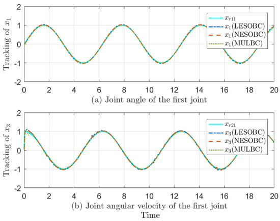
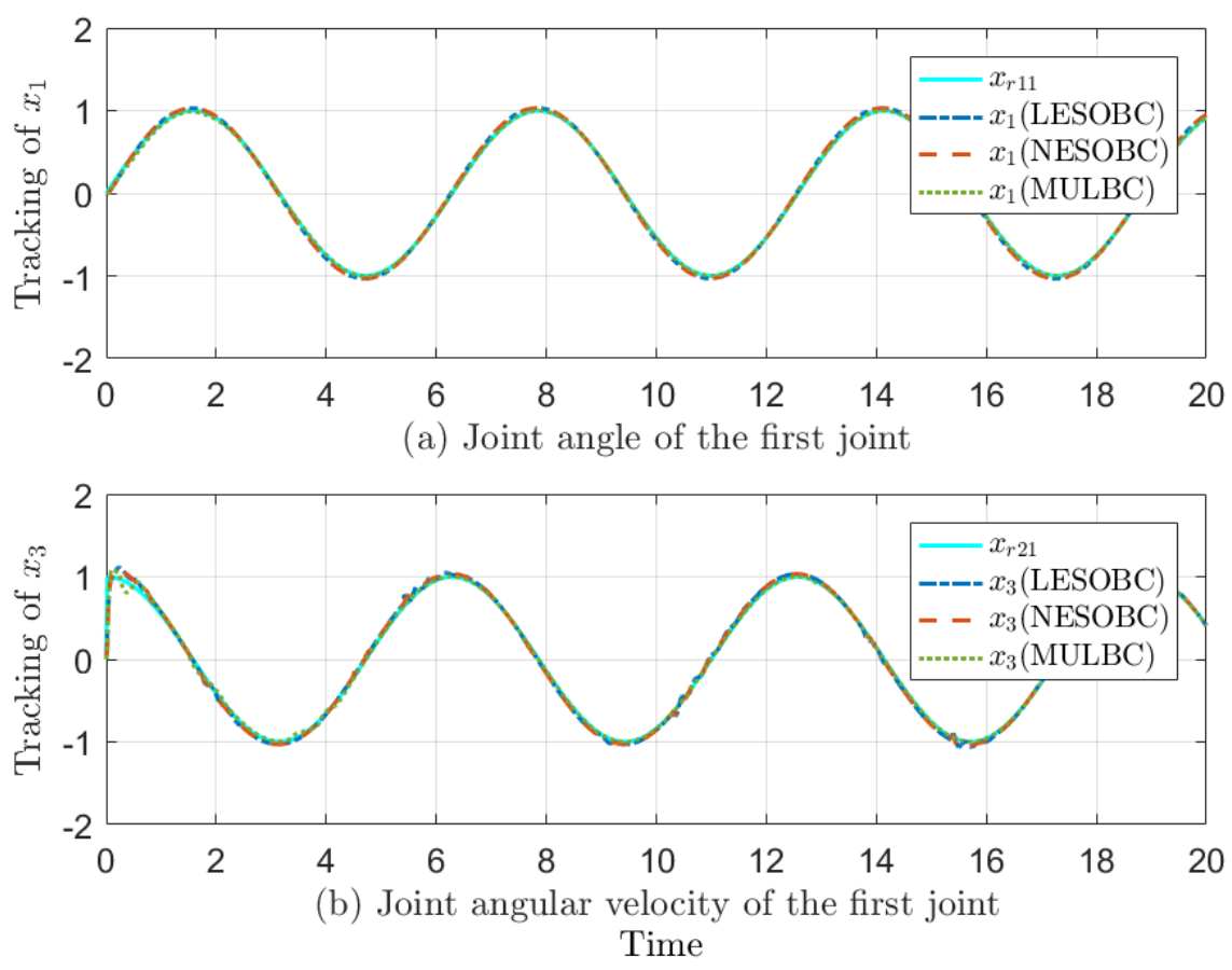
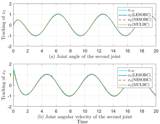
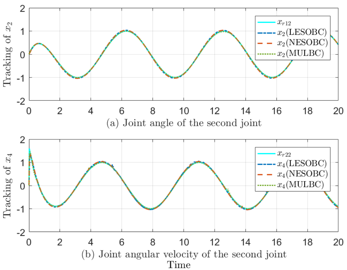
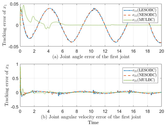
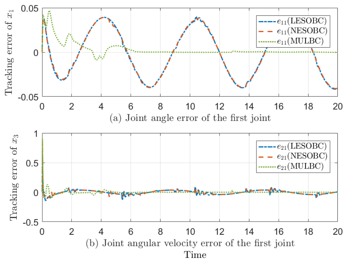
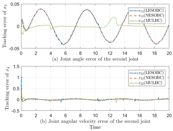
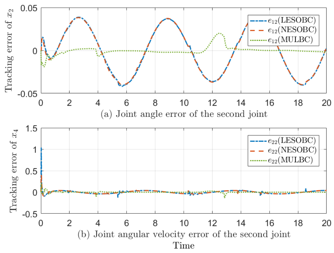
Figure 3 and Figure 4 are the state trajectory tracking curves of the two joints of the two-degrees-of-freedom manipulator, respectively, and Figure 5 and Figure 6 are the state trajectory tracking error curves of the two joints, respectively. It can be seen from the local graph of the state trajectory tracking diagram that the state trajectory of MULBC control method was more consistent with the reference trajectory. It can also be seen from the local figure of the angular velocity tracking of the two joints that the LESOBC control method had undesirable jumping behavior, leading to greater deviation. As can be seen from Figure 5, the tracking error of MULBC quickly converges to near zero value, which is almost zero after 6 s. However, LESOBC and NESOBC control methods both have periodic fluctuation errors, and their tracking error curves tend to be consistent. As can be seen from Figure 6, the tracking error of the MULBC control method was still the smallest, but the error deviation occurred around 12 s; however, it was soon adjusted to a small neighborhood of zero, which had the characteristics of fast response.

Figure 3. State trajectory tracking curves of joint 1.

Figure 4. State trajectory tracking curves of joint 2.

Figure 5. Error curves of state trajectory tracking of joint 1.

Figure 6. Error curves of state trajectory tracking of joint 2.

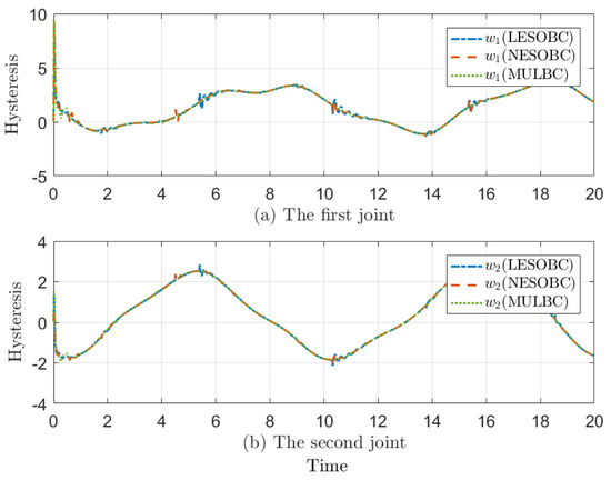
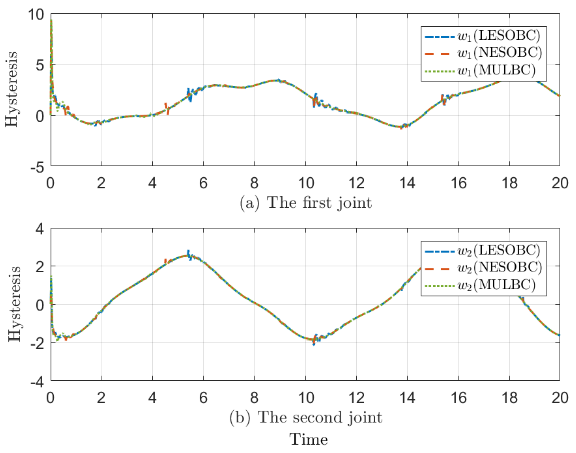
Figure 7 shows the hysteresis characteristic curves of the three control methods. It can be seen that the curve of MULBC is smoother. As can be seen from the local graph, MULBC’s signal could enter the stationary phase faster, while LESOBC and NESOBC control signals had some unexpected oscillations.

Figure 7. Hysteresis characteristic curves.

5.2. Experimental Task of Six-Axis Cooperative Manipulator

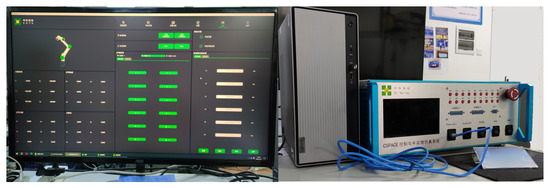
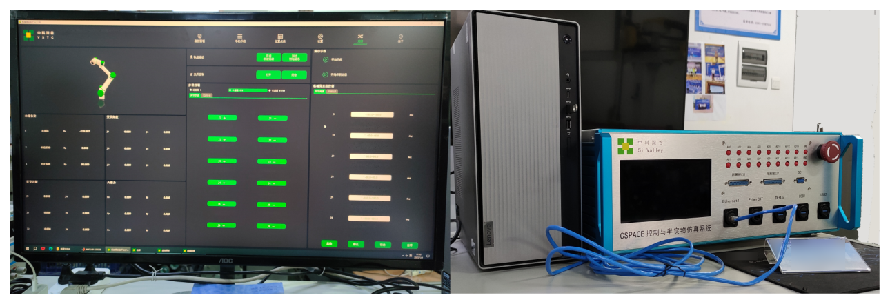
In the experiment, the six-axis cooperative manipulator of Si Valley (Hefei, China) was used to verify the designed control algorithm. The compiled file was passed into the control box by EtherCAT through the compilation of the Simulink control model, and then the actual manipulator was controlled. The hardware configuration is shown in Figure 8:

Figure 8. Hardware configuration.

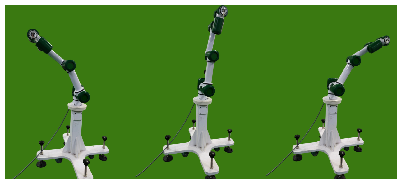
Similarly, the LESOBC and NESOBC control methods were considered as comparison schemes. We enabled the second joint and the third joint of the six-axis cooperative manipulator in Figure 9, and we verified the control algorithm on these two joints with reference trajectories $r_2$ and $r_3$, respectively. It is worth noting that the fourth, fifth and sixth joints of the cooperative manipulator constituted loads that affected the movement of the manipulator:

$$r_2=r_3=0.5sin\left(0.5t\right)$$

Figure 9. The motion process of the manipulator.

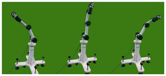
The motion mode of the manipulator during the experiment is shown in Figure 9. The hardware controller adopted the same parameter settings as those specified for the simulation. The comparison controllers were empirically tuned using the same tracking-performance criteria, with common parameters kept consistent where applicable. LESOBC and NESOBC employed the same observer bandwidth of ${\omega }_0=100$. The experimental data were recorded at a sampling interval of $10\mathrm{ms}$, corresponding to a recording frequency of $100\mathrm{Hz}$. As shown in Table 2, the cumulative errors of the two joints are respectively shown, from which it can be seen that no matter which joint, the designed MULBC controller had significantly smaller errors and better performance.

Table 2. Comparison of performance indexes of the three control methods.

	LESOBC	NESOBC	MULBC
$J_1$ (Joint 2, position)	58.7196	60.5329	25.8571
$J_1$ (Joint 3, position)	39.8357	47.5246	34.3602

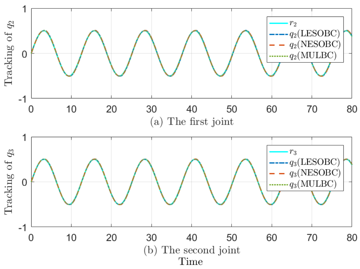
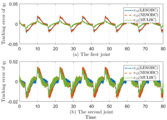
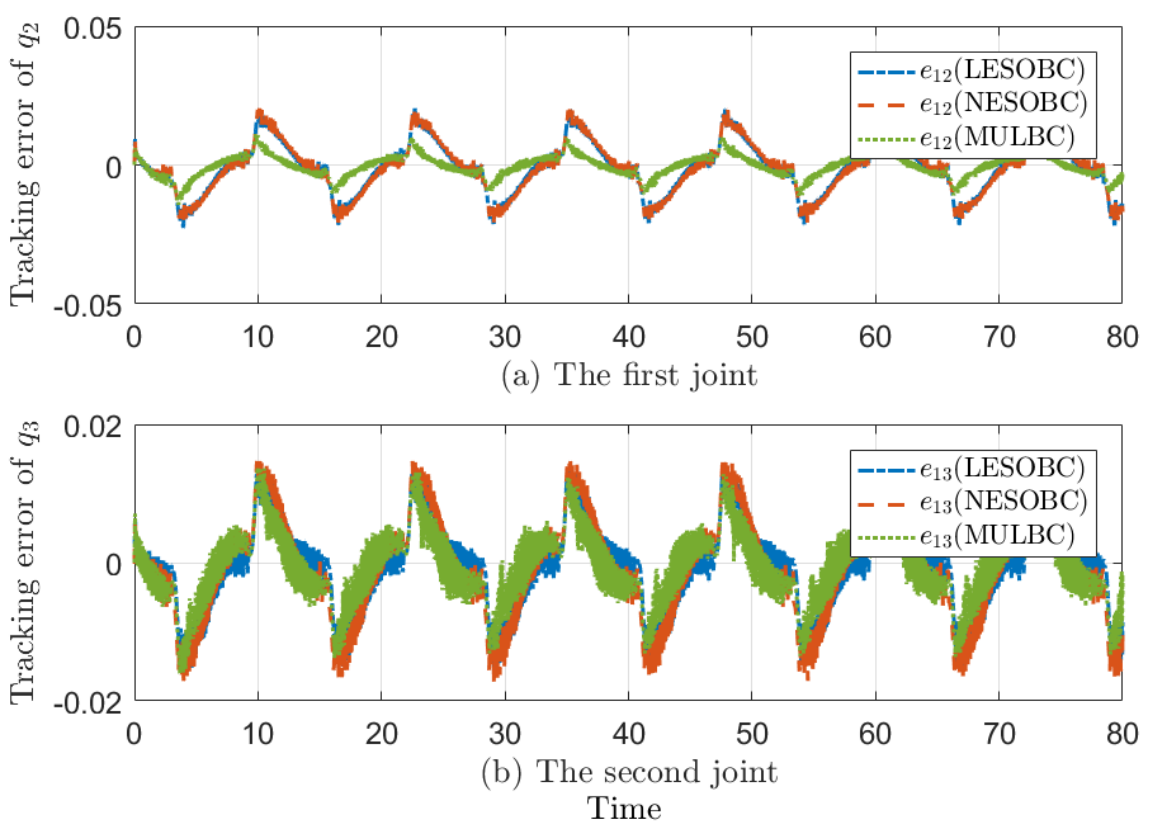
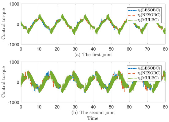
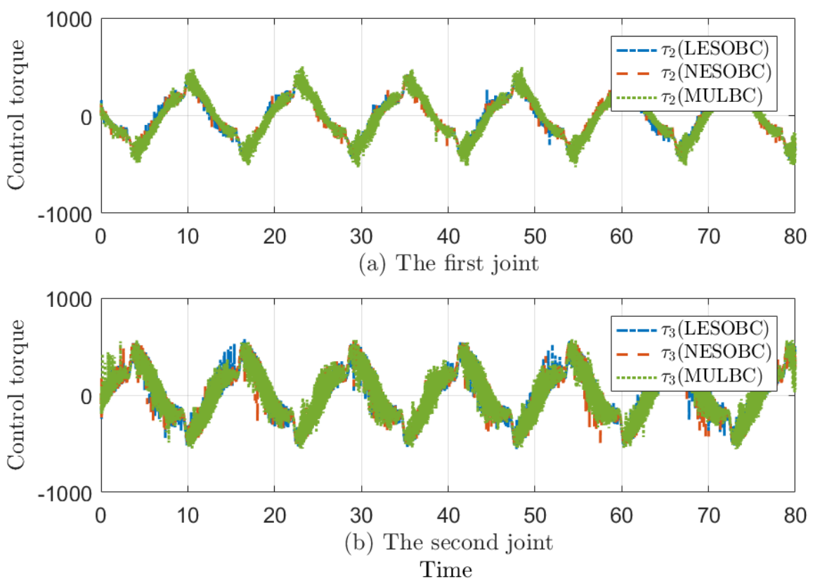
Figure 10 depicts the state trajectory tracking effect under the three controllers, and it can be seen that the selected two joints could track the reference trajectory well. The corresponding tracking error is shown in Figure 11. It can be clearly seen that the proposed MULBC control method had the smallest error nearly all the time. Figure 12 presents the scaled joint control-torque signals of the two actively controlled joints. The plotted signals were obtained by multiplying the actual joint torques (in $\mathrm{N}·\mathrm{m}$) by a factor of 20. Therefore, the plotted values of approximately $\pm 600$ correspond to actual joint torques of approximately $\pm 30\mathrm{N}·\mathrm{m}$. The three controllers exhibited generally consistent torque-response trends.

Figure 10. State trajectory tracking curves.

Figure 11. Error curves of state trajectory tracking.

Figure 12. Control torque curves.

Based on the above results, MULBC demonstrated favorable trajectory-tracking performance under the investigated experimental conditions.

5.3. Limitations

The present simulation and experimental evaluations were limited to the specified reference trajectories, disturbance conditions, and payload configurations. The effects of independently varying reference amplitude and frequency, disturbance magnitude, payload, saturation level, and hysteresis parameters have not been systematically investigated. Repeated trials and statistical dispersion measures were not included. Furthermore, measurement noise was excluded under Assumption 4, and noise robustness was not evaluated. Therefore, the reported results should be interpreted within the investigated operating conditions. A more comprehensive robustness and repeatability evaluation, including parameter re-tuning when necessary, will be considered in future work.

6. Conclusions

Considering the problems of hysteresis, input saturation, external disturbances, model uncertainty, and inertia-matrix uncertainty, a multilateral learning adaptive control strategy was designed based on the model reference adaptive control framework. The high gain PD controller is designed for the linear reference system and is used as the first control component of the nonlinear dynamic system. Based on the state and tracking errors of the nonlinear dynamic system, the state error feedback control law was designed as the second control component of the nonlinear dynamic system. A multilateral learning adaptive mechanism is proposed and is designed to compensate for lumped uncertainties, and the multilateral learning result is regarded as the third control component of the nonlinear dynamic system. The initial value selection of multilateral uncertainty and multilateral weight parameters was studied. A multilateral learning adaptive mechanism was designed to update multilateral uncertainty estimates and weight parameters online according to the tracking and fitting errors. The second-order linear filter is used to obtain the differential signal of the control quantity and tracking error. To address the problem caused by excessively rapid parameter variations, the saturation conversion function is designed to constrain the rate of change of weight parameters within the specified range.

Controllers based on the linear extended state observer and the nonlinear extended state observer were adopted as comparison schemes. A sinusoidal reference trajectory was used for the trajectory-tracking simulations and experiments. Under the investigated simulation and experimental conditions, MULBC achieved smaller cumulative tracking errors than the selected comparison controllers. However, these results do not establish robustness across independently varied operating conditions. Future research could be carried out from two aspects: first, future work will consider challenges such as friction and actuator failures in nonlinear dynamic systems, and it will evaluate the controller under more complex operating conditions; second, the controller will be extended to a wider range of nonlinear systems and more complex application scenarios. Regarding the first aspect, practical nonlinear dynamic systems may involve additional factors not considered in this study, such as friction and actuator failures. These factors require further investigation to improve the reliability of the controller in practical applications. As for the second aspect, nonlinear systems exist widely in various fields. In future work, the proposed controller can be further extended to networked, switched, and stochastic systems to improve its applicability.

References

- Hu, Y.; Yan, H.; Zhang, H.; Wang, M.; Zeng, L. Robust adaptive fixed-time sliding-mode control for uncertain robotic systems with input saturation. IEEE Trans. Cybern. 2023, 53, 2636–2646. [Google Scholar] [CrossRef] [Scilit] [PubMed]
- Jia, S.; Shan, J. Finite-time trajectory tracking control of space manipulator under actuator saturation. IEEE Trans. Ind. Electron. 2020, 67, 2086–2096. [Google Scholar] [CrossRef] [Scilit]
- Hu, J.; Wang, P.; Xu, C.; Zhou, H.; Yao, J. High accuracy adaptive motion control for a robotic manipulator with model uncertainties based on multilayer neural network. Asian J. Control 2022, 24, 1503–1514. [Google Scholar] [CrossRef] [Scilit]
- Gao, M.; Ding, L.; Jin, X. Elm-based adaptive faster fixed-time control of robotic manipulator systems. IEEE Trans. Neural Netw. Learn. Syst. 2023, 34, 4646–4658. [Google Scholar] [CrossRef] [Scilit] [PubMed]
- Ren, Y.; Zhao, Z.; Zhang, C.; Yang, Q.; Hong, K.-S. Adaptive neural-network boundary control for a flexible manipulator with input constraints and model uncertainties. IEEE Trans. Cybern. 2021, 51, 4796–4807. [Google Scholar] [CrossRef] [Scilit] [PubMed]
- Zhao, W.; Liu, Y.; Yao, X. Adaptive fuzzy containment and vibration control for multiple flexible manipulators with model uncertainties. IEEE Trans. Fuzzy Syst. 2023, 31, 1315–1326. [Google Scholar] [CrossRef] [Scilit]
- Baek, S.; Baek, J.; Kwon, W.; Han, S. An adaptive model uncertainty estimator using delayed state-based model-free control and its application to robot manipulators. IEEE/ASME Trans. Mechatron. 2022, 27, 4573–4584. [Google Scholar] [CrossRef] [Scilit]
- Tutsoy, O.; Barkana, D.E. Model free adaptive control of the under-actuated robot manipulator with the chaotic dynamics. ISA Trans. 2021, 118, 106–115. [Google Scholar] [CrossRef] [Scilit] [PubMed]
- Shi, D.; Zhang, J.; Sun, Z.; Xia, Y. Adaptive sliding mode disturbance observer-based composite trajectory tracking control for robot manipulator with prescribed performance. Nonlinear Dyn. 2022, 109, 2693–2704. [Google Scholar] [CrossRef] [Scilit]
- Zhan, B.; Jin, M.; Liu, J. Extended-state-observer-based adaptive control of flexible-joint space manipulators with system uncertainties. Adv. Space Res. 2022, 69, 3088–3102. [Google Scholar] [CrossRef] [Scilit]
- Liu, K.; Chai, Y.; Sun, Z.; Li, Y. An adaptive iterative learning control approach based on disturbance estimation for manipulator system. Int. J. Adv. Rob. Syst. 2019, 16, 1729881419852197. [Google Scholar] [CrossRef] [Scilit]
- Lin, G.; Shan, B.; Ma, Y.; Tian, X.; Yu, J. Adaptive neural network command filtered backstepping impedance control for uncertain robotic manipulators with disturbance observer. Trans. Inst. Meas. Control 2022, 44, 799–808. [Google Scholar] [CrossRef] [Scilit]
- Fan, Y.; Yang, C.; Zhan, H.; Li, Y. Neuro-adaptive-based predefined-time smooth control for manipulators with disturbance. IEEE Trans. Syst. Man. Cybern. Syst. 2024, 54, 4605–4616. [Google Scholar] [CrossRef] [Scilit]
- Wu, Y.; Huang, R.; Li, X.; Liu, S. Adaptive neural network control of uncertain robotic manipulators with external disturbance and time-varying output constraints. Neurocomputing 2019, 323, 108–116. [Google Scholar] [CrossRef] [Scilit]
- Peng, J.; Ding, S.; Dubay, R. Adaptive composite neural network disturbance observer-based dynamic surface control for electrically driven robotic manipulators. Neural Comput. Appl. 2021, 33, 6197–6211. [Google Scholar] [CrossRef] [Scilit]
- Zhou, X.; Wang, H.; Tian, Y. Adaptive boundary iterative learning vibration control using disturbance observers for a rigid-flexible manipulator system with distributed disturbances and input constraints. J. Vib. Control 2022, 28, 1324–1340. [Google Scholar] [CrossRef] [Scilit]
- Shi, D.; Zhang, J.; Sun, Z.; Shen, G.; Xia, Y. Composite trajectory tracking control for robot manipulator with active disturbance rejection. Control Eng. Pract. 2021, 106, 104670. [Google Scholar] [CrossRef] [Scilit]
- Zhu, Q.; Shang, H.; Lu, X.; Chen, Y. Adaptive sliding mode tracking control of underwater vehicle-manipulator systems considering dynamic disturbance. Ocean Eng. 2024, 291, 116300. [Google Scholar] [CrossRef] [Scilit]
- Zhang, J.; Xia, M.; Li, S.; Liu, Z.; Yang, J. The adaptive bilateral control of underwater manipulator teleoperation system with uncertain parameters and external disturbance. Electronics 2024, 13, 1122. [Google Scholar] [CrossRef] [Scilit]
- Chen, Y.; Liang, J.; Wu, Y.; Miao, Z.; Zhang, H.; Wang, Y. Adaptive sliding-mode disturbance observer-based finite-time control for unmanned aerial manipulator with prescribed performance. IEEE Trans. Cybern. 2023, 53, 3263–3276. [Google Scholar] [CrossRef] [Scilit] [PubMed]
- He, W.; Amoateng, D.O.; Yang, C.; Gong, D. Adaptive neural network control of a robotic manipulator with unknown backlash-like hysteresis. IET Control Theory Appl. 2017, 11, 567–575. [Google Scholar] [CrossRef] [Scilit]
- Kharrat, M.; Krichen, M.; Alkhalifa, L.; Gasmi, K. Neural networks-based adaptive command filter control for nonlinear systems with unknown backlash-like hysteresis and its application to single link robot manipulator. AIMS Math. 2024, 9, 959–973. [Google Scholar] [CrossRef] [Scilit]
- Chen, J.; Zhang, H.; Zhu, T.; Pan, S. Trajectory tracking control of a manipulator based on an immune algorithm-optimized neural network in the presence of unknown backlash-like hysteresis. Appl. Math. Comput. 2024, 470, 128552. [Google Scholar] [CrossRef] [Scilit]
- Wang, X.; Yin, X.; Wu, Q.; Meng, F. Adaptive neural tracking control for nonstrict-feedback nonlinear systems with unknown backlash-like hysteresis and unknown control directions. Int. J. Robust. Nonlinear Control 2018, 28, 5140–5157. [Google Scholar] [CrossRef] [Scilit]
- Ahmed, S.; Wang, H.; Tian, Y. Adaptive high-order terminal sliding mode control based on time delay estimation for the robotic manipulators with backlash hysteresis. IEEE Trans. Syst. Man. Cybern. Syst. 2021, 51, 1128–1137. [Google Scholar] [CrossRef] [Scilit]
- Wang, H.; Fang, L.; Wang, J.; Song, T.; Shen, H. Adaptive neural sliding mode control with prescribed performance of robotic manipulators subject to backlash hysteresis. Proc. Inst. Mech. Eng. Part C J. Mech. Eng. Sci. 2022, 236, 1826–1837. [Google Scholar] [CrossRef] [Scilit]
- Zhang, Y.; Fang, L.; Song, T.; Zhang, M. Model-free adaptive control based on prescribed performance and time delay estimation for robotic manipulators subject to backlash hysteresis. Proc. Inst. Mech. Eng. Part C J. Mech. Eng. Sci. 2023, 237, 5674–5691. [Google Scholar] [CrossRef] [Scilit]
- Anjum, Z.; Zhou, H.; Guo, Y. Self-tuning fuzzy nonsingular proportional-integral-derivative type fast terminal sliding mode control for robotic manipulator in the presence of backlash hysteresis. Trans. Inst. Meas. Control 2022, 44, 809–819. [Google Scholar] [CrossRef] [Scilit]
- Abhari, S.A.; Hashemzadeh, F.; Baradarannia, M.; Kharrati, H. An adaptive robust control scheme for robot manipulators with unknown backlash nonlinearity in gears. Trans. Inst. Meas. Control 2019, 41, 2789–2802. [Google Scholar] [CrossRef] [Scilit]
- Zhou, X.; Wang, H.; Tian, Y. Neural network state observer-based robust adaptive iterative learning output feedback control for the rigid-flexible coupled robotic systems with unknown delays and backlash-like hysteresis. Nonlinear Dyn. 2022, 110, 1515–1542. [Google Scholar] [CrossRef] [Scilit]
- Zhou, B.; Yang, L.; Wang, C.; Lai, G.; Chen, Y. Adaptive finite-time tracking control of robot manipulators with multiple uncertainties based on a low-cost neural approximator. J. Frankl. Inst.—Eng. Appl. Math. 2022, 359, 4938–4958. [Google Scholar] [CrossRef] [Scilit]
- Shang, D.; Li, X.; Yin, M.; Li, F. Model identification control strategy for coupled elastic joint flexible load drive system based on nnsmc controller and new deformation description. J. Frankl. Inst.—Eng. Appl. Math. 2023, 360, 6357–6401. [Google Scholar] [CrossRef] [Scilit]
- Han, C.; Qin, K.; Lin, B.; Shi, M.; Li, Z.; Liu, Q. Neural network-based distributed consensus tracking control for uncertain euler-lagrange systems over directed topologies. Neurocomputing 2024, 608, 128383. [Google Scholar] [CrossRef] [Scilit]
- Wang, Y.; Li, S.; Wang, D.; Ju, F.; Chen, B.; Wu, H. Adaptive time-delay control for cable-driven manipulators with enhanced nonsingular fast terminal sliding mode. IEEE Trans. Ind. Electron. 2021, 68, 2356–2367. [Google Scholar] [CrossRef] [Scilit]
- Wang, Y.; Yan, F.; Jiang, S.; Chen, B. Adaptive nonsingular terminal sliding mode control of cable-driven manipulators with time delay estimation. Int. J. Syst. Sci. 2020, 51, 1429–1447. [Google Scholar] [CrossRef] [Scilit]
- Wang, Y.; Chen, J.; Zhu, K.; Chen, B.; Wu, H. Practical tracking control of cable-driven robots using adaptive nonsingular fast terminal sliding mode. IEEE Access 2018, 6, 68057–68069. [Google Scholar] [CrossRef] [Scilit]
- Yang, Q.; Ma, X.; Wang, W.; Peng, D. Adaptive non-singular fast terminal sliding mode trajectory tracking control for robot manipulators. Electronics 2022, 11, 3672. [Google Scholar] [CrossRef] [Scilit]
- Izadbakhsh, A.; Khorashadizadeh, S. Robust task-space control of robot manipulators using differential equations for uncertainty estimation. Robotica 2017, 35, 1923–1938. [Google Scholar] [CrossRef] [Scilit]
- Gholipour, R.; Fateh, M.M. Robust control of robotic manipulators in the task-space using an adaptive observer based on chebyshev polynomials. J. Syst. Sci. Complex. 2020, 33, 1360–1382. [Google Scholar] [CrossRef] [Scilit]
- Izadbakhsh, A.; Khorashadizadeh, S. Robust adaptive control of robot manipulators using bernstein polynomials as universal approximator. Int. J. Robust. Nonlinear Control 2020, 30, 2719–2735. [Google Scholar] [CrossRef] [Scilit]
- Izadbakhsh, A. An observer-based output tracking controller for electrically driven cooperative multiple manipulators with adaptive bernstein-type approximator. Robotica 2022, 40, 2295–2319. [Google Scholar] [CrossRef] [Scilit]
- Fang, L.; Zhang, Y.; Song, T. Tracking control for robotic manipulators with prescribed performance and adaptive sliding mode disturbance observer. Trans. Inst. Meas. Control 2024, 46, 2378–2390. [Google Scholar] [CrossRef] [Scilit]
- Shen, H.; Song, T.; Fang, L.; Wang, H.; Zhang, Y. Adaptive super twisting observer-based prescribed time integral sliding mode tracking control of uncertain robotic manipulators. Int. J. Adapt. Control Signal Process. 2024, 38, 2588–2616. [Google Scholar] [CrossRef] [Scilit]
- Duc Thien, T.; Ahn, K.K. Finite-time fault-tolerant control for a robotic manipulator with output constraint and uncertainties. IEEE Access 2021, 9, 146771–146782. [Google Scholar] [CrossRef] [Scilit]
- Duc Thien, T.; Jin, M.; Ahn, K.K. Nonlinear extended state observer based on output feedback control for a manipulator with time-varying output constraints and external disturbance. IEEE Access 2019, 7, 156860–156870. [Google Scholar] [CrossRef] [Scilit]
- Tran, D.T.; Dao, H.V.; Ahn, K.K. Adaptive synchronization sliding mode control for an uncertain dual-arm robot with unknown control direction. Appl. Sci. 2023, 13, 7423. [Google Scholar] [CrossRef] [Scilit]
- Kong, L.; Lai, Q.; Ouyang, Y.; Li, Q.; Zhang, S. Neural learning control of a robotic manipulator with finite-time convergence in the presence of unknown backlash-like hysteresis. IEEE Trans. Syst. Man. Cybern. Syst. 2022, 52, 1916–1927. [Google Scholar] [CrossRef] [Scilit]
Disclaimer/Publisher’s Note: The statements, opinions and data contained in all publications are solely those of the individual author(s) and contributor(s) and not of MDPI and/or the editor(s). MDPI and/or the editor(s) disclaim responsibility for any injury to people or property resulting from any ideas, methods, instructions or products referred to in the content. |
© 2026 by the authors. Licensee MDPI, Basel, Switzerland. This article is an open access article distributed under the terms and conditions of the Creative Commons Attribution (CC BY) license.