Discrete-Element Modelling of Bedding- and Stress-Controlled Hydraulic Fracturing in Deep Qiongzhusi Shale

Abstract

The Cambrian Qiongzhusi Formation shale of the Sichuan Basin, buried below 4000 m, is a key deep-shale-gas target whose hydraulic fracturing is jointly controlled by bedding weak planes and high in situ stress. This study separates the two controls quantitatively and establishes a reproducible criterion for selecting favourable bedding attitudes and scaling treatment energy. A fluid–solid coupled discrete-element model was built on PFC2D, combining parallel-bond matrix contacts, smooth-joint bedding planes installed on a discrete fracture network, servo-controlled stress boundaries and a cubic-law fluid network, with micromechanical parameters calibrated against a triaxial test on a core from a 4601.76 m depth. Seven bedding inclinations (0–90°) were simulated under a unified stress state, and nine stress combinations were arranged in a 3 × 3 orthogonal design of basal horizontal stress (88.1–125 MPa) and vertical–horizontal stress difference (0.1–6 MPa) at a fixed 60° bedding, then analysed by quadratic response surface and two-way ANOVA. The peak fracturing pressure follows a U-shaped relation with bedding inclination spanning 110–160 MPa. Low-angle bedding (0–30°) favours lateral extension (ratios: 0.63–0.68) but limits vertical connectivity, whereas high-angle bedding (75–90°) promotes vertical breakthrough with lateral reach falling to 0.08–0.09. Ranked by a composite stimulation score built from four normalised sub-scores—initiation efficiency, lateral reach, vertical reach and an SRV proxy—60° is the optimum (S = 0.76), ahead of 15° (0.72) and 45° (0.67), combining the lowest fracturing pressure of 110 MPa with progressive branching rather than sudden breakthrough. Raising basal σh from 88.1 to 125 MPa lengthens propagation approximately fourfold and shifts the failure mode from tensile splitting to shear–tensile ductile rupture, with the tensile-fracture proportion falling from 1.0 to 0.25–0.35. The two-way ANOVA attributes 82–99% of the variance of every response to σh (p ≤ 0.031), whereas the stress difference contributes at most 8.2% and reaches significance for none (p > 0.17) The bedding optimum is placed on a stated objective function rather than qualitative judgement, and the two stress controls are shown to combine additively rather than multiplicatively within the Qiongzhusi stress envelope. Practically, treatment energy should be scaled with basal σ_h rather than with the stress difference, and target intervals selected at 45–60° bedding.

1. Introduction

The Cambrian Qiongzhusi Formation of the Sichuan Basin has been identified over the past decade as one of the most important replacement plays for shale-gas exploitation in China, particularly in the Weiyuan–Ziyang region where favourable structural conditions coincide with substantial organic-matter content and considerable formation thickness. As the shallower Silurian Longmaxi Formation has entered a mature stage of development, the Chinese natural-gas industry has progressively shifted attention to deeper and older shale-gas systems in order to sustain reserve growth and productivity increases. The Qiongzhusi Formation, whose burial depths in the target intervals typically exceed 4000 m, is now regarded as a strategic resource for this next stage of Chinese unconventional gas development [1,2,3]. However, the transition from the Longmaxi to the Qiongzhusi play introduces a considerably more difficult geomechanical environment: greater burial depth, stronger diagenetic modification, more compact rock matrix, higher feldspar and clay content, denser development of natural weak planes, and pronounced multi-directional stress differences. Under these conditions, the hydraulic-fracturing process—which is essential for economic exploitation of low-permeability shale—becomes considerably more complex, and fracture initiation, deflection, branching, and coalescence deviate substantially from the patterns observed in shallower Longmaxi wells [4,5,6,7].

Compared with the Longmaxi Formation, the Qiongzhusi Formation was deposited significantly earlier and has undergone more extensive tectonic reworking and diagenesis, so the shale matrix is more compact, natural pore–fracture connectivity is weaker, and closure stresses are considerably higher. Fracturing fluid injected under these conditions must overcome both the mechanical closure stress required to open a fracture and the path-selection effects imposed by the interaction between the propagating tip and the pre-existing bedding surfaces, microfractures, and grain boundaries that pervade the rock mass. Whether a near-wellbore fracture can be transformed into a spatially complex, hydraulically conductive network directly determines the stimulated reservoir volume and hence long-term well productivity [8,9,10]. In the Qiongzhusi target intervals, laminated fabrics and diagenetic layering give rise to widely varying weak-plane densities, while the local stress regime combines high absolute magnitudes with moderate vertical–horizontal stress differences; the resulting fracturing response varies markedly between sub-layers of a single well and cannot be captured by any single evaluation parameter.

Conventional fracability evaluation relies on indicators such as the mineral brittleness index, uniaxial compressive strength, Young’s modulus, Poisson’s ratio, fracture toughness, natural-fracture density, and horizontal stress difference [5,6,10]. These are useful for first-pass screening but cannot describe how a fracture evolves as it propagates into the far field, nor resolve the coupled influence of weak-plane structure and stress state on the geometry of the resulting network. Field and laboratory observations both show that high mineral brittleness does not necessarily produce a complex network, and that a dense population of weak planes does not always increase the stimulated volume: weak planes may promote branching and enhance connectivity, or may absorb the fracture through bedding-parallel slip and restrict height growth. Lumping these competing effects into a single scalar discards precisely the mechanistic information needed for treatment design.

Whether a fracture crosses a bedding interface, deflects along it, or bifurcates depends on a competition between the crack-tip stress state, the cohesive strength and post-debonding friction of the interface, and the far-field stress combination—a competition formalised in the Renshaw–Pollard crossing criterion [11] and extended through experiments on layered shales [12,13]. Repeated deflection, re-initiation, and layer crossing can build a network with substantial lateral and vertical extent, whereas fluid energy consumed mainly by slip along a single dominant weak plane limits network development [14,15]. Resolving these process-level interactions requires a numerical framework in which fracture paths are not predefined. The discrete-element method, introduced by Cundall and Strack [16] and developed into the bonded-particle model by Potyondy and Cundall [17], represents rock as a discontinuous particle assembly connected by breakable contacts, supporting the natural formation of new fracture surfaces, the explicit representation of bedding weak planes as smooth-joint contacts, and the emergent behaviour of networks in heterogeneous rock [18,19]. It has been applied successfully to coupled hydro-mechanical simulation in shale, natural-fracture systems, and geothermal reservoirs [20,21,22,23,24,25,26].

On this basis, the present study builds a coupled DEM hydraulic-fracturing model of Qiongzhusi shale on PFC2D, with bedding weak planes represented by a discrete fracture network combined with smooth-joint contacts, in situ stress imposed through servo-controlled walls, and micromechanical parameters calibrated against triaxial-compression tests on a core from a 4601.76 m depth. Seven bedding inclinations and nine stress combinations arranged in a three-level orthogonal design are examined. Two aspects distinguish the analysis from previous bedding-and-stress studies. The bedding optimum is determined by an explicit composite scoring rubric rather than by qualitative comparison, so that the ranking of attitudes is reproducible; the two stress controls are separated by response-surface fitting and analysis of variance, so that their contributions to each response can be quantified and tested rather than inferred. The results are used to inform target-interval screening and treatment design for the deep Qiongzhusi shale.

2. Materials and Methods

2.1. Governing Equations of the Particle-Based DEM Framework

The Qiongzhusi Formation shale is characterised by a complex mineralogical assemblage, strongly heterogeneous distribution of natural weak planes, pronounced vertical layering, and high-magnitude three-dimensional in situ stress. During hydraulic fracturing, the initiation, deflection, layer crossing, and branching of induced fractures are not governed by any single control—brittleness, weak-plane density, or stress difference—but by the coupled action of mineral composition, weak-plane structure, and stress state. To capture this coupling explicitly, the present work employs the particle-based discrete-element method as implemented in PFC2D.

In the DEM, the rock is discretised into an assembly of rigid circular particles connected by breakable inter-particle contacts, and its overall deformation and failure under external loading are represented by the composite response of particle translation, particle rotation, contact deformation, and contact breakage. For any particle i, translational and rotational motions obey Newton’s second law:

$$m_{\mathrm{i}}{\displaystyle \frac{d^2{u}_{\mathrm{i}}}{d{t}^2}}=F_{\mathrm{i}}; I_{\mathrm{i}}{\displaystyle \frac{d{\omega }_{\mathrm{i}}}{dt}}=M_{\mathrm{i}}$$

(1)

where $m_{\mathrm{i}}$ denotes the particle mass, $u_{\mathrm{i}}$ is the particle position vector, $F_{\mathrm{i}}$ is the resultant contact force acting on the particle from its neighbours and from external boundaries, $I_{\mathrm{i}}$ is the moment of inertia, ${\omega }_{\mathrm{i}}$ is the angular velocity, and $M_{\mathrm{i}}$ is the resultant moment.

Equation (1) is integrated forward in time by an explicit velocity-Verlet scheme with a critical timestep governed by the stiffest particle mass–stiffness pair in the assembly. Because the timestep must be sufficiently small to remain stable, DEM simulations of hydraulic fracturing are typically computationally intensive; the choice of a two-dimensional PFC2D framework in the present study represents a compromise between computational cost and the resolution required to represent the interaction between weak planes and the propagating fracture.

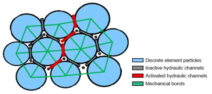
Between matrix particles, cementation is represented by the linear parallel-bond (PB) model of Potyondy and Cundall [17]. In this model, a finite-radius bond is installed at the contact between two particles, and both force and moment increments are transmitted through the bond as the particles undergo relative displacement. The bond incrementally accumulates normal, shear, and bending stresses; when either the maximum tensile stress exceeds the tensile strength σ_t or the maximum shear stress exceeds the cohesive shear strength τ_c, the bond breaks irreversibly. Bond breakage in tension registers a tensile microcrack at the contact, while breakage in shear registers a shear microcrack. After breakage, a residual frictional contact governed by Coulomb’s law persists between the two particles, transmitting compressive normal and frictional shear forces only. This constitutive setup allows the PB model to reproduce the elastic–brittle failure behaviour characteristic of cemented sedimentary rocks such as shale. The fluid-solid coupling mechanism is illustrated in Figure 1.

Figure 1. Schematic of fluid–solid coupling.

Figure 1. Schematic of fluid–solid coupling.

2.2. Representation of Bedding Weak Planes and Mineral Heterogeneity

For matrix particles, the PB model described above is used to represent cementation failure. To represent bedding weak planes, the smooth-joint (SJ) contact model is installed on top of the standard contact wherever a bond is intersected by a prescribed bedding surface. In the SJ model, contact forces are decomposed and updated independently along the normal and tangential directions of the bedding plane, irrespective of the particle-to-particle line-of-centres. This decomposition enables the model to reproduce the anisotropic slip and opening responses of a smooth planar discontinuity, complementing the continuum description of shale as a transversely isotropic medium [27], and to reproduce laboratory-observed fracture-crossing versus deflection behaviours along bedding.

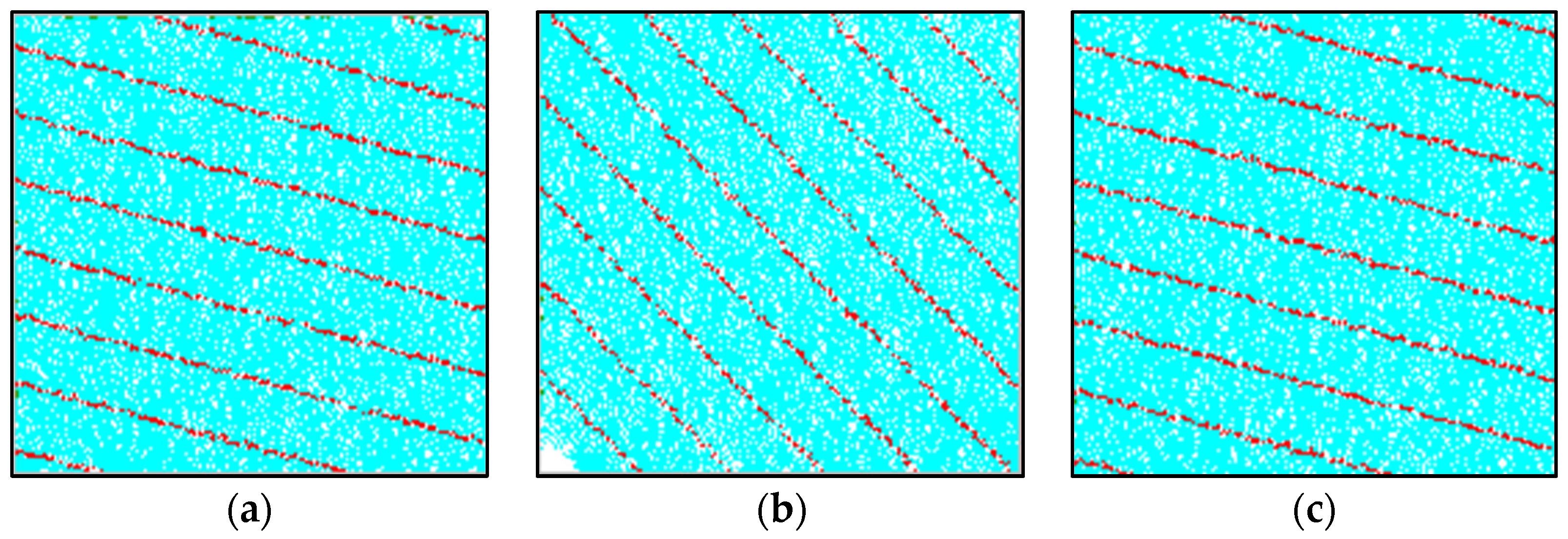
Two distinct model configurations are used in parallel in the present study, as illustrated in Figure 2. (i) In the triaxial-compression model, a zoned layered assignment approach is employed: the specimen is divided evenly along its height into ten alternating layer groups, and the PB parameters at the contacts falling within the inter-layer bands are weakened to represent the reduced strength of bedding. This approach is convenient for calibration because it approximates a real laminated shale specimen and, because no explicit joint elements are introduced, preserves the compact matrix response that dominates a triaxial test at high confinement. (ii) In the hydraulic-fracturing model, an explicit discrete fracture network (DFN) is used to represent bedding: using FISH programming in PFC2D, seven main bedding fractures together with four buffer fractures on each side—fifteen fractures in total—are generated uniformly through the specimen at the prescribed inclination angle. The spacing of the main bedding fractures equals the specimen width divided by seven, and the length of each fracture is set to 1.5 times the specimen width to ensure that every bedding surface fully traverses the specimen boundaries. The SJ contact model is then automatically installed at every particle contact intersected by a bedding surface, so that each bedding surface behaves as an anisotropic weak plane with an independent set of normal stiffness, shear stiffness, cohesion, tensile strength, friction coefficient, and friction angle. Mineral heterogeneity is represented indirectly by grouping matrix particles into strong, medium, and weak clusters through spatial variation in the PB parameters, with cluster ratios chosen to reproduce the observed vertical variability of Qiongzhusi mineralogy. Different bedding dip angles were set for subsequent parametric analysis, as illustrated in Figure 3.

Figure 2. DEM numerical models used in the present study: (a) triaxial-compression model with ten alternating layer groups; (b) hydraulic-fracturing model with DFN-based bedding and smooth-joint contacts installed at intersections.

Figure 2. DEM numerical models used in the present study: (a) triaxial-compression model with ten alternating layer groups; (b) hydraulic-fracturing model with DFN-based bedding and smooth-joint contacts installed at intersections.

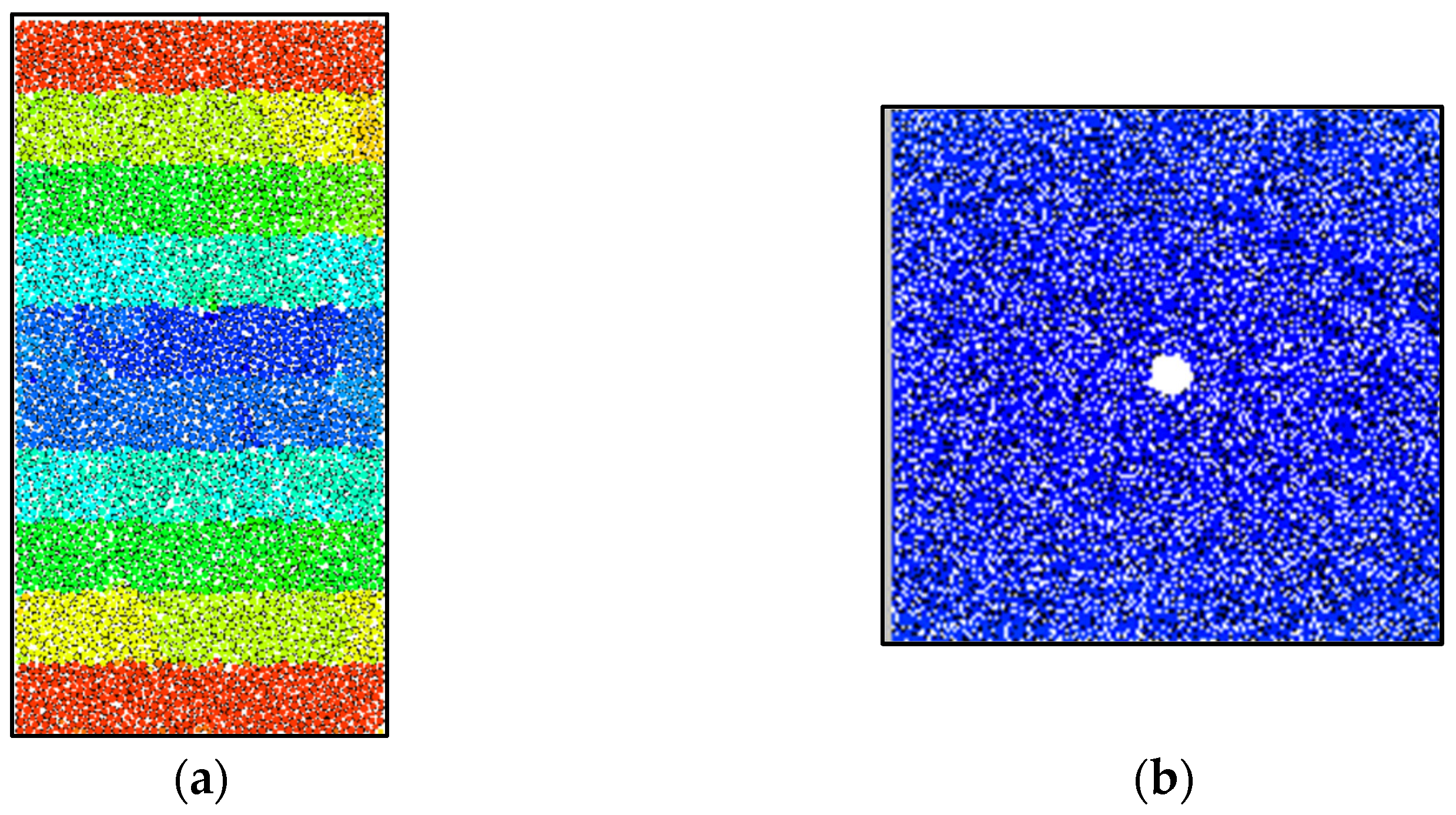
Figure 3. DFN construction of the hydraulic-fracturing model at different bedding inclinations: (a) 75°; (b) 45°; (c) 15°. Seven main bedding fractures plus four buffer fractures on each side are generated with a length equal to 1.5 times the specimen width.

Figure 3. DFN construction of the hydraulic-fracturing model at different bedding inclinations: (a) 75°; (b) 45°; (c) 15°. Seven main bedding fractures plus four buffer fractures on each side are generated with a length equal to 1.5 times the specimen width.

2.3. Initialisation of In Situ Stress and Fluid–Solid Coupling

Initial in situ stresses are applied through a servo-control scheme built on the four rigid walls that bound the specimen. A dedicated FISH function evaluates the wall–particle contact forces at every timestep, converts them into internal stress components ${\sigma }_{\mathrm{x}\mathrm{x}}$ and ${\sigma }_{\mathrm{y}\mathrm{y}}$ through division by the corresponding contact area, and adjusts the wall velocity increment according to the difference between the measured stress and the prescribed target stress:

$$v_{\mathrm{w}\mathrm{a}\mathrm{l}\mathrm{l}}=G·\left({\sigma }_{\mathrm{m}\mathrm{e}\mathrm{a}\mathrm{s}\mathrm{u}\mathrm{r}\mathrm{e}\mathrm{d}}-{\sigma }_{\mathrm{t}\mathrm{a}\mathrm{r}\mathrm{g}\mathrm{e}\mathrm{t}}\right)$$

(2)

where v_wall is the wall velocity increment and G is a servo gain parameter chosen small enough to ensure numerical stability during the stress build-up stage. The horizontal and vertical stresses inside the specimen converge to their target values after several thousand timesteps. The vertical stress represents the effective overburden and the horizontal stress represents the effective minimum horizontal principal stress. Once the target stresses are reached, the wall velocities are frozen and the specimen is considered to be in a state of pre-fracturing equilibrium.

Hydraulic-fracturing simulation is carried out using the built-in fluid-network model of PFC2D. The interstitial voids between particles are automatically identified and organised into a network of pore domains connected by throats; the pore domains are treated as reservoirs of fluid pressure, and the throats are treated as one-dimensional conduits in which fluid flow is driven by the pressure difference between the adjacent pore domains. Fluid flow through each throat obeys the cubic law:

$$q={\displaystyle \frac{a^3}{12\mu }}·{\displaystyle \frac{\mathsf{\Delta }p}{L}}$$

(3)

where q is the volumetric flow rate through the throat, a is the hydraulic aperture that depends on the local particle spacing and the residual aperture parameter, μ is the fluid dynamic viscosity, Δp is the pressure difference driving the flow, and L is the throat length. At each timestep, the pore pressure inside each pore domain is updated according to the mass balance between fluid inflow, fluid outflow, and change in pore volume:

$$\mathsf{\Delta }{p}_{\mathrm{p}\mathrm{o}\mathrm{r}\mathrm{e}}={\displaystyle \frac{K_{\mathrm{f}}}{V_{\mathrm{p}}}}·\left(\mathsf{\Sigma }q\mathsf{\Delta }t-\mathsf{\Delta }{V}_{\mathrm{p}}\right)$$

(4)

where $K_{\mathrm{f}}$ is the bulk modulus of the fracturing fluid, $V_{\mathrm{p}}$ is the pore volume, and Δ$V_{\mathrm{p}}$ is its increment over the timestep. The updated pore pressure exerts a hydraulic force on the surrounding particles, which is added to the mechanical force balance of Equation (1). In this way, the fluid-network model provides two-way coupling between the fluid pressure field and the mechanical response of the particle assembly: bond breakage locally increases the hydraulic aperture and hence the local permeability, and the redistributed fluid pressure feeds back into the mechanical force balance to drive further breakage.

2.4. Triaxial-Compression Test and Calibration Scheme

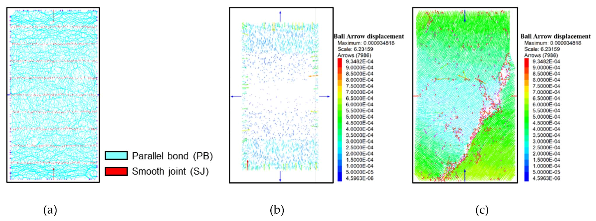
The triaxial calibration model adopts the same contact system as the subsequent hydraulic-fracturing models: parallel bonds represent the shale matrix and smooth-joint contacts represent the bedding planes. The two model families therefore differ only in specimen geometry and loading path, not in the constitutive representation, so the calibrated parameters transfer directly. The triaxial-compression numerical test used for micromechanical calibration is composed of two loading stages. In the first stage, the servo-control system described in Section 2.3 drives the horizontal and vertical walls simultaneously to the prescribed confining-pressure target and holds them stable, thereby establishing an isotropic stress state inside the specimen that matches the laboratory confining pressure. In the second stage, the vertical servo control is switched off, and a constant velocity is imposed on the top and bottom walls so that the specimen is loaded axially in displacement control. The velocity is chosen small enough to ensure a quasi-static loading rate and to avoid dynamic effects. Loading continues until the axial stress falls to 80% of the peak strength during the post-peak phase, so that the full pre-peak elastic response, the non-linear pre-peak yielding, the peak strength, and the post-peak softening branch are all captured in one continuous simulation. Throughout the test, the axial stress, axial strain, and radial strain are recorded, and the failure pattern is visualised by mapping the location and orientation of every broken bond onto the specimen at predefined snapshots. The specific workflow is illustrated in Figure 4.

Figure 4. Loading scheme of the triaxial-compression numerical test: (a) layered-joint model; (b) confining-pressure application; (c) simulated fracture pattern at the end of the test.

Figure 4. Loading scheme of the triaxial-compression numerical test: (a) layered-joint model; (b) confining-pressure application; (c) simulated fracture pattern at the end of the test.

The calibration of the matrix PB parameters is based on the triaxial-compression results of a Qiongzhusi shale core sample from the fifth sub-layer at a 4601.76 m depth (core number: RE-01). The laboratory reference values are summarised in Table 1: overburden pressure of 117.3 MPa, confining pressure of 100.9 MPa, pore pressure of 88.0 MPa, fracture pressure of 393.51 MPa, Young’s modulus at 3.925 × 10⁴ MPa, and Poisson’s ratio at 0.224. Through an iterative parameter-adjustment procedure, the effective elastic modulus at the parallel-bond contacts (pb-emod), the stiffness ratio (pb-kratio), the tensile strength (pb-ten), the cohesive shear strength (pb-coh), the friction angle (pb-fa), the coefficient of inter-particle friction (fric), and the gap-related parameters were successively updated until the simulated uniaxial compressive strength and Young’s modulus fell within 10% of the laboratory reference. The SJ parameters of the bedding planes were then calibrated jointly against the peak strength, Young’s modulus, and Poisson’s ratio of the triaxial test.

Table 1. Laboratory triaxial mechanical results of the Qiongzhusi calibration sample RE-01.

Core No.	Overburden Pressure (MPa)	Confining Pressure (MPa)	Pore Pressure (MPa)	Fracture Pressure (MPa)	Young’s Modulus (1010 Pa)	Poisson’s Ratio
RE-01	117.3	100.9	88.0	393.51	3.925	0.224

Four candidate parameter combinations were designed to bracket the measured mechanical response, corresponding to plausible variations in parallel-bond stiffness ratio, tensile-to-cohesive strength ratio, and disc-element effective modulus (Table 2). The four sets share the same friction angle (45°), inter-particle friction coefficient (0.8), and SJ parameters (kn = 1.2 × 10¹³ Pa/m, ks = 2.0 × 10¹² Pa/m, tensile strength at 1.8 × 10⁷ Pa, cohesion of 7.0 × 10⁶ Pa), and differ mainly in the parallel-bond parameters that most strongly influence Young’s modulus and peak strength.

Table 2. Four candidate micromechanical parameter sets designed for triaxial calibration.

Sample	pb-emod (GPa)	pb-kratio	pb-ten (MPa)	pb-coh (MPa)	sj-kn (GPa/m)	sj-ks (GPa/m)
No. 1	40	1.7	350	180	12,000	2000
No. 2	50	2.2	250	335	12,000	2000
No. 3	50	2.5	400	235	12,000	2000
No. 4	60	2.5	400	235	12,000	2000

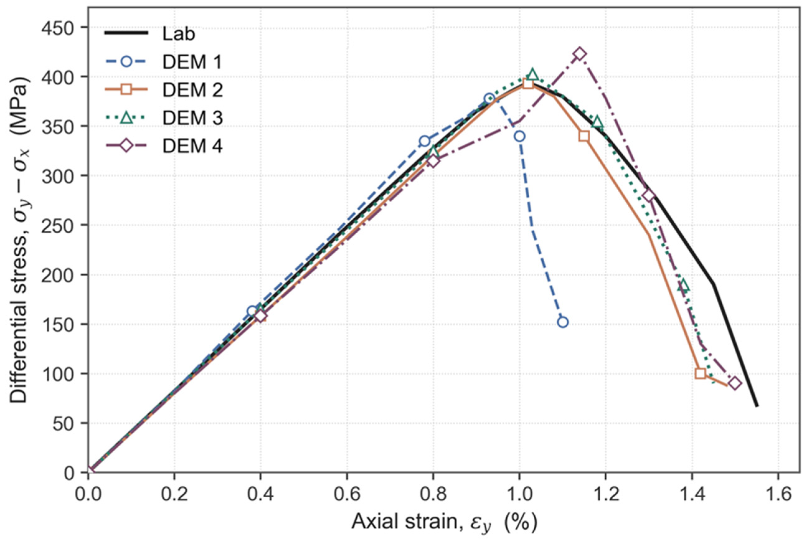
The simulated stress–strain responses of the four candidate sets are compared with the laboratory reference curve in Figure 5 and Figure 6. Overall, all four numerical curves reproduce the three characteristic phases of shale triaxial behaviour—linear elastic loading, non-linear yielding, and post-peak softening—and their overall trends agree well with the laboratory curve. In the linear elastic phase, the initial slopes of the four curves are close to that of the laboratory curve, indicating that the calibrated matrix parallel-bond elastic-modulus parameter is reliable (Table 3). In terms of peak strength, the four samples give peak values of 378 MPa (No. 1), 393 MPa (No. 2), 403 MPa (No. 3), and 423 MPa (No. 4). Relative to the laboratory value of 393.51 MPa, Sample No. 2 matches the reference most closely; Sample No. 3 overestimates the peak by approximately 2.4%; Sample No. 1 underestimates it by approximately 3.9%; and Sample No. 4 overestimates it by approximately 7.5% of the laboratory value. In the post-peak softening branch, the drop rate of Sample No. 1 is closest to the laboratory curve, but its peak strain is slightly smaller than the laboratory value. Sample No. 2 reproduces the position of the peak strain most accurately, and its post-peak softening trend is also closest to the laboratory result. Based on the combined evaluation of peak strength, peak-strain position, and post-peak softening character, Sample No. 2 delivers the highest overall fidelity to the Qiongzhusi triaxial behaviour, and its parameter set is therefore adopted as the input for the subsequent hydraulic-fracturing simulations.

Table 3. Simulated versus measured triaxial mechanical responses for the four candidate parameter sets.

Sample	Poisson’s Ratio	Young’s Modulus (1010 Pa)	Fracture Pressure (MPa)
RE-01	0.224	3.925	393.51
1	0.20	4.25	378
2	0.22	3.89	393
3	0.22	3.91	403
4	0.23	3.82	423

Table 3. Simulated versus measured triaxial mechanical responses for the four candidate parameter sets.

Sample	Poisson’s Ratio	Young’s Modulus (1010 Pa)	Fracture Pressure (MPa)
RE-01	0.224	3.925	393.51
1	0.20	4.25	378
2	0.22	3.89	393
3	0.22	3.91	403
4	0.23	3.82	423

Figure 5. Simulated failure pattern and stress–strain responses of the four candidate samples: (a) Sample 1; (b) Sample 2; (c) Sample 3; (d) Sample 4.

Figure 5. Simulated failure pattern and stress–strain responses of the four candidate samples: (a) Sample 1; (b) Sample 2; (c) Sample 3; (d) Sample 4.

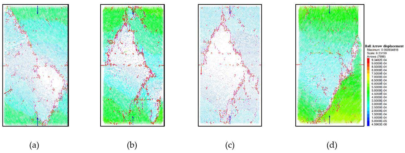
Figure 6. Comparison of the differential stress–axial strain curves obtained from the four DEM calibration samples.

Figure 6. Comparison of the differential stress–axial strain curves obtained from the four DEM calibration samples.

2.5. Simulation Programme for Bedding-Angle and Stress Sensitivity

The first family, presented in Section 3.1, is a bedding-angle series covering seven bedding inclinations (0°, 15°, 30°, 45°, 60°, 75°, and 90°) under a unified stress state. The effective minimum horizontal stress is fixed at σ_h,eff = 12.9 MPa and the effective vertical stress at σ_v,eff = 20.0 MPa; superposed on a pore pressure of 88.0 MPa, these correspond to total in situ stresses of σ_h = 100.9 MPa and σ_v = 108.0 MPa, which reproduce the confining pressure and loading state of the calibration core RE-01 and ensure that the geomechanical background of the fracturing simulations is anchored to the actual Qiongzhusi deep-shale environment. The simulation parameters are listed in Table 4. In the two-dimensional implementation these two components are applied to the horizontal and vertical servo walls and are denoted σ_x and σ_y respectively, so that σ_x ≡ σ_h,eff and σ_y ≡ σ_v,eff throughout. In every case, the injection rate is held constant at 1 × 10⁻⁵ m²/s (in the two-dimensional specific-injection sense).

The second family, presented in Section 3.2, is a three-level orthogonal stress design anchored on the field-stress envelope of the Qiongzhusi Formation. As summarised in Table 5, the minimum horizontal principal stress σ_h (total) averages approximately 105.33 MPa with a range of 85.00–124.70 MPa, and the vertical–horizontal stress difference σ_v − σ_h averages approximately 2.68 MPa with a range of 0.10–6.40 MPa. Based on this envelope, three basal horizontal-stress levels (nominally 88.1, 105, 125 MPa as total in situ stress) and three vertical–horizontal stress differences (0.1, 3, 6 MPa) are combined orthogonally to yield nine loading combinations (Table 6, cases YL-1 to YL-9). This design isolates two variables—basal stress level and vertical–horizontal stress difference—while keeping the reservoir structural model unchanged, so that their independent and combined effects on fracture network evolution can be quantified.

The pore pressure is held at the calibration value of 88.0 MPa in all nine cases, so that the effective stress applied to the PFC2D specimen equals the total in situ stress minus 88.0 MPa. Because the field lower bound σ_h = 85 MPa would correspond to a slightly negative effective stress under this pore pressure, the −1 basal level is clamped upward to a total σ_h of 88.1 MPa (effective σ_h = 0.1 MPa), so that the effective horizontal stress remains non-negative and physically meaningful at the lower factor level. Because the two-dimensional PFC2D framework represents only a single horizontal stress component, the horizontal stress difference σ_H − σ_h cannot be varied independently in-plane and is therefore held aside; the design treats the basal horizontal stress σ_h and the vertical–horizontal stress difference σ_v − σ_h as the two orthogonal control variables. For each case, the total σ_h, total σ_v, fixed pore pressure, and the effective σ_h and σ_v actually applied to the model (denoted σ_x and σ_y in the 2D implementation) are listed in Table 6. Throughout the nine stress cases the bedding structure is held fixed at an inclination of 60°, with the same DFN geometry, spacing, and smooth-joint parameters as in the bedding series of Section 3.1. This is the attitude identified in Section 3.1.2 as the highest composite stimulation score delivery, so the stress sensitivity is examined on the configuration of greatest engineering interest, and the responses reported in Section 3.2 are attributable to the stress boundary alone.

The complete parameter set adopted for both simulation families is summarised in Table 4. The PB parameters are inherited directly from Sample No. 2’s calibration; the SJ parameters are those calibrated jointly against the peak strength and Poisson’s ratio; the fluid-network parameters (perm, flow_dt, flow_given, ro_rad) are chosen to reproduce a fracturing-fluid viscosity and bulk-modulus regime representative of slickwater fracturing operations in the Qiongzhusi play. All simulations use the same specimen dimensions (100 mm × 100 mm), the same particle-size distribution (mean radius of 0.35 mm with a uniform range of ±20%), and the same fluid-injection scheme, so that the effects observed between cases can be attributed unambiguously to the corresponding change in bedding angle or stress state.

Table 4. Complete parameter set of the hydraulic-fracturing model.

Group	Parameter	Value
PB	pb-emod (Pa)	5.0 × 1010
PB	pb-kratio	2.2
PB	pb-ten (Pa)	2.5 × 108
PB	pb-coh (Pa)	3.35 × 108
PB	pb-fa (°)	45
PB	fric	0.8
PB	de-emod (Pa)	4.0 × 1010
SJ	sj-kn (Pa/m)	1.2 × 1013
SJ	sj-ks (Pa/m)	2.0 × 1012
SJ	sj-fric	0.8
SJ	sj-ten (Pa)	1.8 × 107
SJ	sj-coh (Pa)	7.0 × 106
SJ	sj-fa (°)	45
SJ	sj-large	1
Fluid	Perm(Pa−1·s−1)	1 × 10−3
Fluid	flow_dt (s)	1 × 10−5
Fluid	flow_given (m2/s)	1 × 10−5
Fluid	ro_rad (m)	5 × 10−3

Table 4. Complete parameter set of the hydraulic-fracturing model.

Group	Parameter	Value
PB	pb-emod (Pa)	5.0 × 1010
PB	pb-kratio	2.2
PB	pb-ten (Pa)	2.5 × 108
PB	pb-coh (Pa)	3.35 × 108
PB	pb-fa (°)	45
PB	fric	0.8
PB	de-emod (Pa)	4.0 × 1010
SJ	sj-kn (Pa/m)	1.2 × 1013
SJ	sj-ks (Pa/m)	2.0 × 1012
SJ	sj-fric	0.8
SJ	sj-ten (Pa)	1.8 × 107
SJ	sj-coh (Pa)	7.0 × 106
SJ	sj-fa (°)	45
SJ	sj-large	1
Fluid	Perm(Pa−1·s−1)	1 × 10−3
Fluid	flow_dt (s)	1 × 10−5
Fluid	flow_given (m2/s)	1 × 10−5
Fluid	ro_rad (m)	5 × 10−3

Table 5. Statistical summary of in situ stress in the Qiongzhusi Formation (all values in MPa).

Statistic	σH	σh	σv	σH − σh	σv − σh
Mean	121.84	105.33	119.16	16.51	2.68
Minimum	99.20	85.00	99.10	13.40	0.10
Maximum	145.10	124.70	139.70	20.40	6.40

Table 5. Statistical summary of in situ stress in the Qiongzhusi Formation (all values in MPa).

Statistic	σH	σh	σv	σH − σh	σv − σh
Mean	121.84	105.33	119.16	16.51	2.68
Minimum	99.20	85.00	99.10	13.40	0.10
Maximum	145.10	124.70	139.70	20.40	6.40

Table 6. Design matrix of the three-level orthogonal stress-sensitivity experiments. The bedding inclination is held at 60° in all nine cases.

Case	h Level	(v − h) Level	Total σh (MPa)	Total σv (MPa)	Pore Pressure (MPa)	σx = σh − Pp (MPa)	σy = σv − Pp (MPa)
YL-1	−1	−1	88.1	88.2	88.0	0.1	0.2
YL-2	−1	0	88.1	91.1	88.0	0.1	3.1
YL-3	−1	1	88.1	94.1	88.0	0.1	6.1
YL-4	0	−1	105.0	105.1	88.0	17.0	17.1
YL-5	0	0	105.0	108.0	88.0	17.0	20.0
YL-6	0	1	105.0	111.0	88.0	17.0	23.0
YL-7	1	−1	125.0	125.1	88.0	37.0	37.1
YL-8	1	0	125.0	128.0	88.0	37.0	40.0
YL-9	1	1	125.0	131.0	88.0	37.0	43.0

Table 6. Design matrix of the three-level orthogonal stress-sensitivity experiments. The bedding inclination is held at 60° in all nine cases.

Case	h Level	(v − h) Level	Total σh (MPa)	Total σv (MPa)	Pore Pressure (MPa)	σx = σh − Pp (MPa)	σy = σv − Pp (MPa)
YL-1	−1	−1	88.1	88.2	88.0	0.1	0.2
YL-2	−1	0	88.1	91.1	88.0	0.1	3.1
YL-3	−1	1	88.1	94.1	88.0	0.1	6.1
YL-4	0	−1	105.0	105.1	88.0	17.0	17.1
YL-5	0	0	105.0	108.0	88.0	17.0	20.0
YL-6	0	1	105.0	111.0	88.0	17.0	23.0
YL-7	1	−1	125.0	125.1	88.0	37.0	37.1
YL-8	1	0	125.0	128.0	88.0	37.0	40.0
YL-9	1	1	125.0	131.0	88.0	37.0	43.0

3. Results

3.1. Effect of Bedding Inclination on Fracture Network Evolution

This section reports the results of the seven-case bedding-angle series and evaluates fracture network evolution through four quantitative indicators: peak fracturing pressure, stress-perturbation area, lateral-extension ratio, and vertical-extension ratio. The four indicators are chosen because they collectively describe the two principal aspects of a stimulated network—initiation threshold and planar extent—and because they can be extracted directly from the DEM output without requiring additional post-processing assumptions. The bedding-angle series therefore constitutes a systematic sensitivity analysis in which the bedding inclination is the single independent variable, and its effect on the fracturing process can be quantified rigorously across the full seven-case range.

3.1.1. Peak Fracturing Pressure

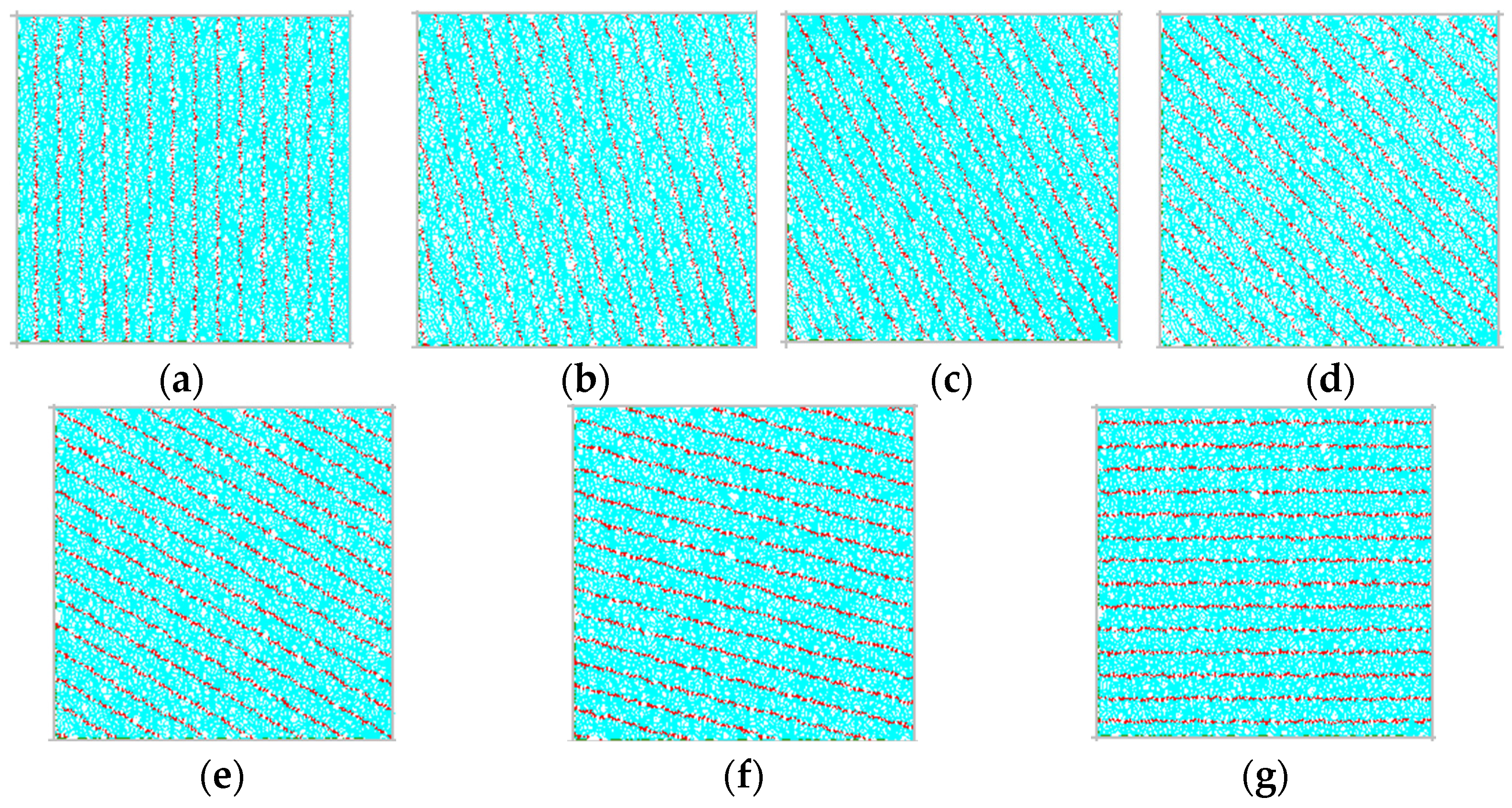
Peak fracturing pressure is the primary indicator of the difficulty of stimulating a reservoir interval; it directly determines the upper limit of pumping-pressure requirements and the feasibility of a treatment programme. In the present work, the peak fracturing pressures for each case are reported as effective values, with the pore pressure of 88 MPa subtracted, so that the values shown correspond to the net effective pressures required to open the fracture. The models for each case are shown in Figure 7 .The resulting distribution across the seven cases is shown in Figure 8 and exhibits a distinctly non-monotonic, roughly U-shaped dependence on bedding inclination, in general agreement with the trend predicted by classical weak-plane theory but with local features that reflect the specific geomechanical characteristics of the Qiongzhusi Formation.

Specifically, the 90° case (near-vertical bedding) delivers an effective fracturing pressure of 120 MPa, at a moderately low level. When the inclination increases to 75°, the fracturing pressure rises to 140 MPa and forms a local peak; this behaviour is related to the fact that the 75° case exposes the bedding surfaces to a large normal effective compressive stress, which increases the resistance to weak-plane activation. As the inclination decreases further to 60°, the fracturing pressure drops sharply to a global minimum of 110 MPa, a fall of 30 MPa relative to the 75° case. This global minimum is a direct expression of the fact that the shear-to-normal-stress ratio on the bedding plane best matches the Mohr–Coulomb slip criterion at this inclination, so that shear activation of the bedding and tensile splitting of the matrix can be triggered simultaneously at a low net pressure, minimising the overall initiation resistance.

Figure 7. Fracture network evolution at different bedding inclinations: (a) 90°; (b) 75°; (c) 60°; (d) 45°; (e) 30°; (f) 15°; (g) 0°.

Figure 7. Fracture network evolution at different bedding inclinations: (a) 90°; (b) 75°; (c) 60°; (d) 45°; (e) 30°; (f) 15°; (g) 0°.

On the other flank of the U-shape, as the inclination decreases from 60° towards 15°, the effective fracturing pressure follows an approximately monotonic increasing trend, taking successive values of 110 MPa (60°), 125 MPa (45°), 145 MPa (30°), and 160 MPa (15°). The global maximum, 160 MPa, is reached at the 15° case, an increase of 50 MPa relative to the global minimum. This trend indicates that as the bedding inclination decreases from 60° towards 15°, the normal effective compressive stress across the bedding plane continues to grow while the tangential shear component along the bedding progressively diminishes, jointly making shear activation of the weak plane progressively more difficult. The 15° case therefore exhibits the strongest resistance to fracturing and the highest pumping-pressure requirement. In the 0–15° range, the fracturing pressure retreats from 160 MPa to 140 MPa, indicating that when the bedding becomes nearly horizontal the geometrical asymmetry between the bedding and the stress field relaxes and the weakening effect of the bedding is partially restored, although the pressure remains higher than in the near-optimal intermediate cases.

Figure 8. Effective peak fracturing pressure as a function of bedding inclination.

Figure 8. Effective peak fracturing pressure as a function of bedding inclination.

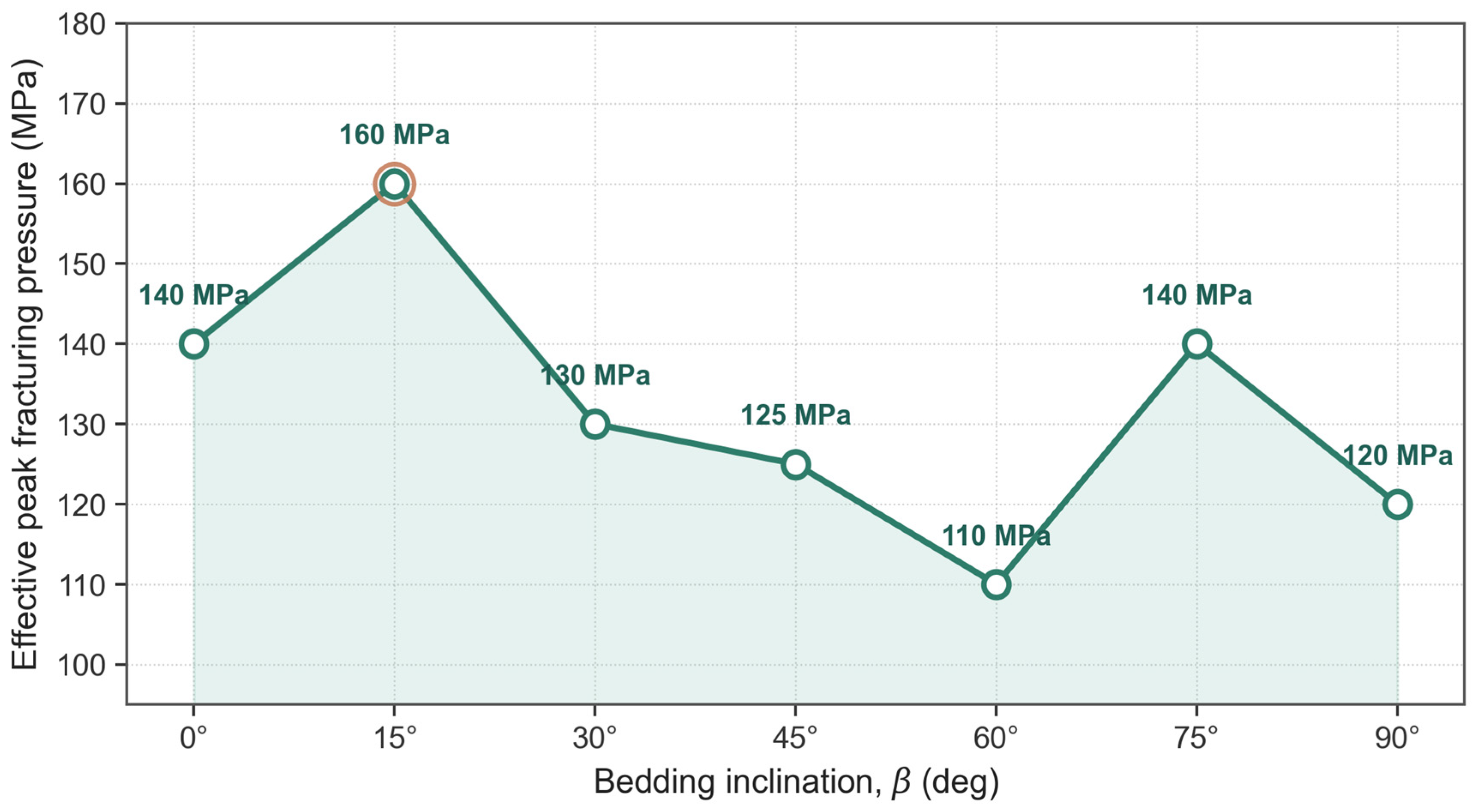
Overall, the seven cases span a range of 50 MPa in effective fracturing pressure, corresponding to a relative variation of approximately 31%. This is a substantial variation that confirms bedding attitude as a key geological factor controlling the fracturing behaviour of the Qiongzhusi Formation. In practical engineering, the bedding inclination of a target sub-layer should therefore be regarded as an essential input for pumping-pressure prediction, and differentiated treatment parameters should be designed for intervals with different bedding attitudes in order to achieve effective stimulation within a reasonable pumping-pressure envelope.

3.1.2. Network Extension and Comprehensive Evaluation

Three complementary indicators—the stress-perturbation area, the lateral-extension ratio, and the vertical-extension ratio—are extracted from the DEM output to characterise the planar and vertical development of the fracture network under each of the seven bedding inclinations.

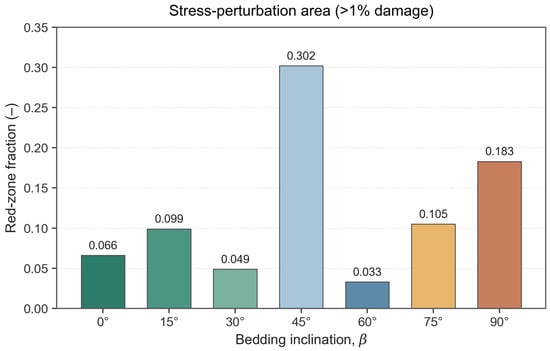
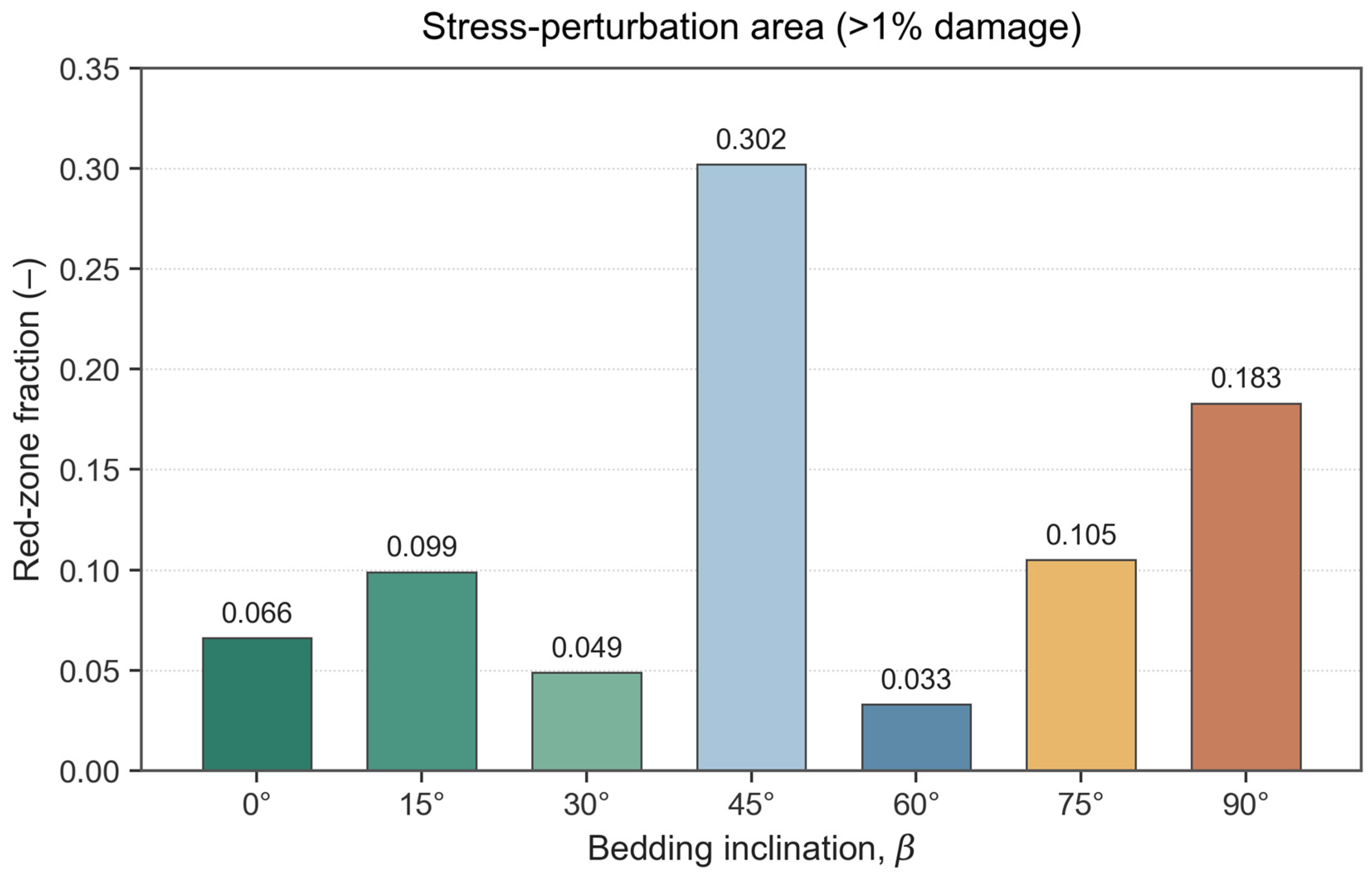
The stress-perturbation area (Figure 9), defined as the areal fraction of the specimen covered by the high-displacement zone in the displacement contour maps, grows monotonically with injection pressure but with widely different magnitudes. It reaches 0.546 at 140 MPa in the 90° case and 0.302 in the 75° case, both far above the 0–60° cases (all below 0.1, with the 0° case at 0.099). The 90–75° dominance is a direct expression of near-vertical bedding: when the beds are close to vertical, the minimum horizontal principal stress acts as their closure stress, so the fluid can wedge open the beds at a relatively low net pressure and drive large-scale particle displacement. A broadly diffused displacement field is not by itself favourable, however—it may indicate an integral, weakly branched failure with limited network complexity.

Figure 9. Evolution of the stress-perturbation area (red-zone fraction) during fracture propagation for different bedding inclinations.

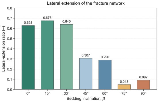
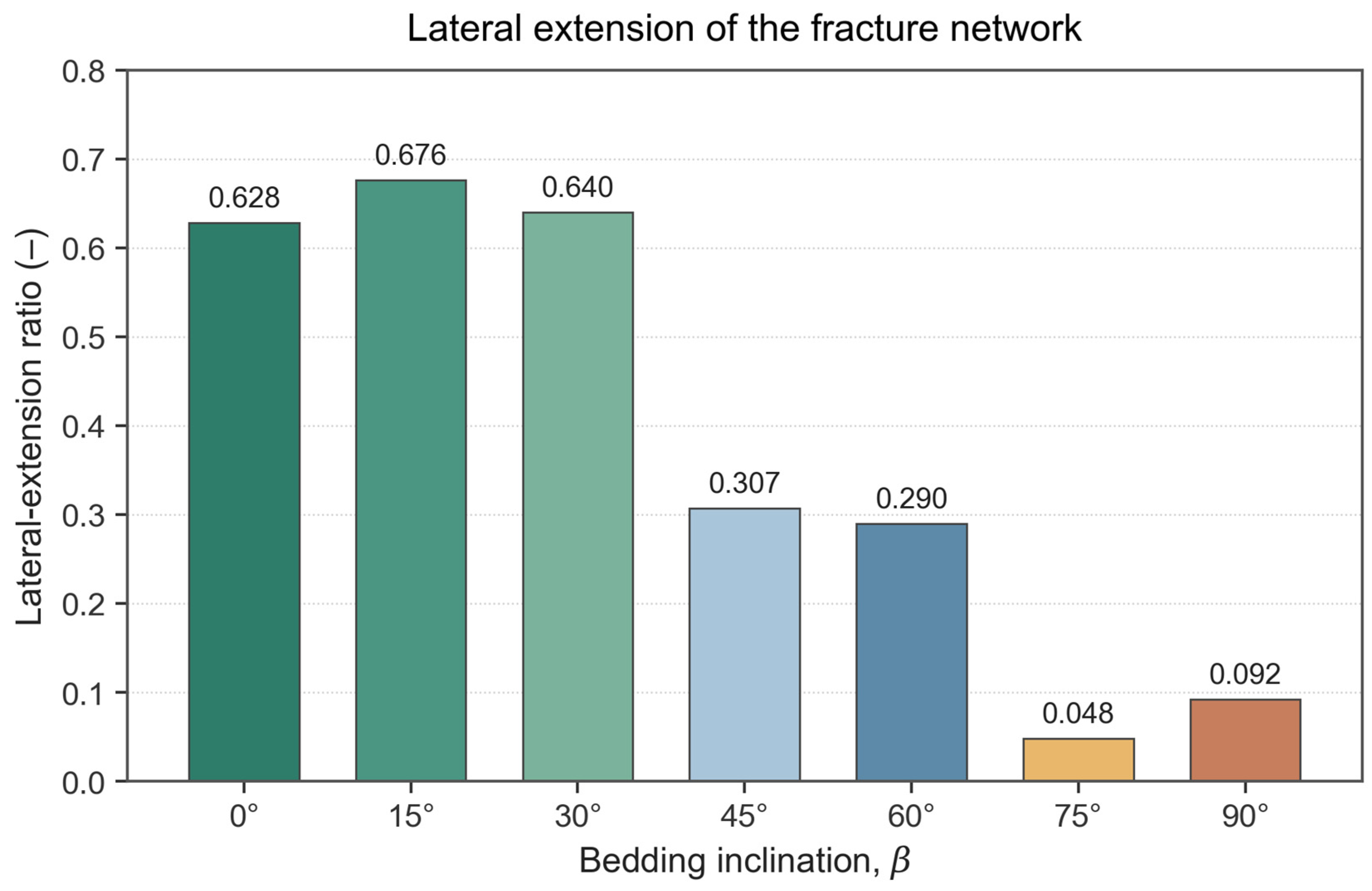
The lateral-extension ratio (Figure 10), measured perpendicular to the maximum horizontal principal stress, shows the opposite pattern. The 0°, 15°, and 30° cases reach the highest values (0.640, 0.676, 0.628), because the near-horizontal bedding is consistently favourable to fluid propagation along bed strike and produces a system dominated by lateral extension. The 45° and 60° cases occupy an intermediate range (0.307, 0.290), while the 75° and 90° cases fall to only 0.092 and 0.081; under high-inclination bedding the injected fluid energy is concentrated on vertical layer-crossing propagation and the horizontal reach of stimulation is severely restricted.

Figure 10. Evolution of the lateral-extension ratio during fracture propagation for different bedding inclinations.

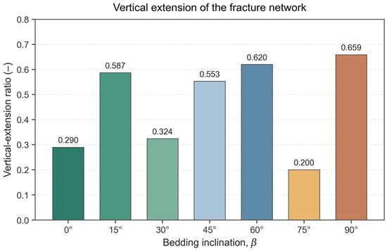
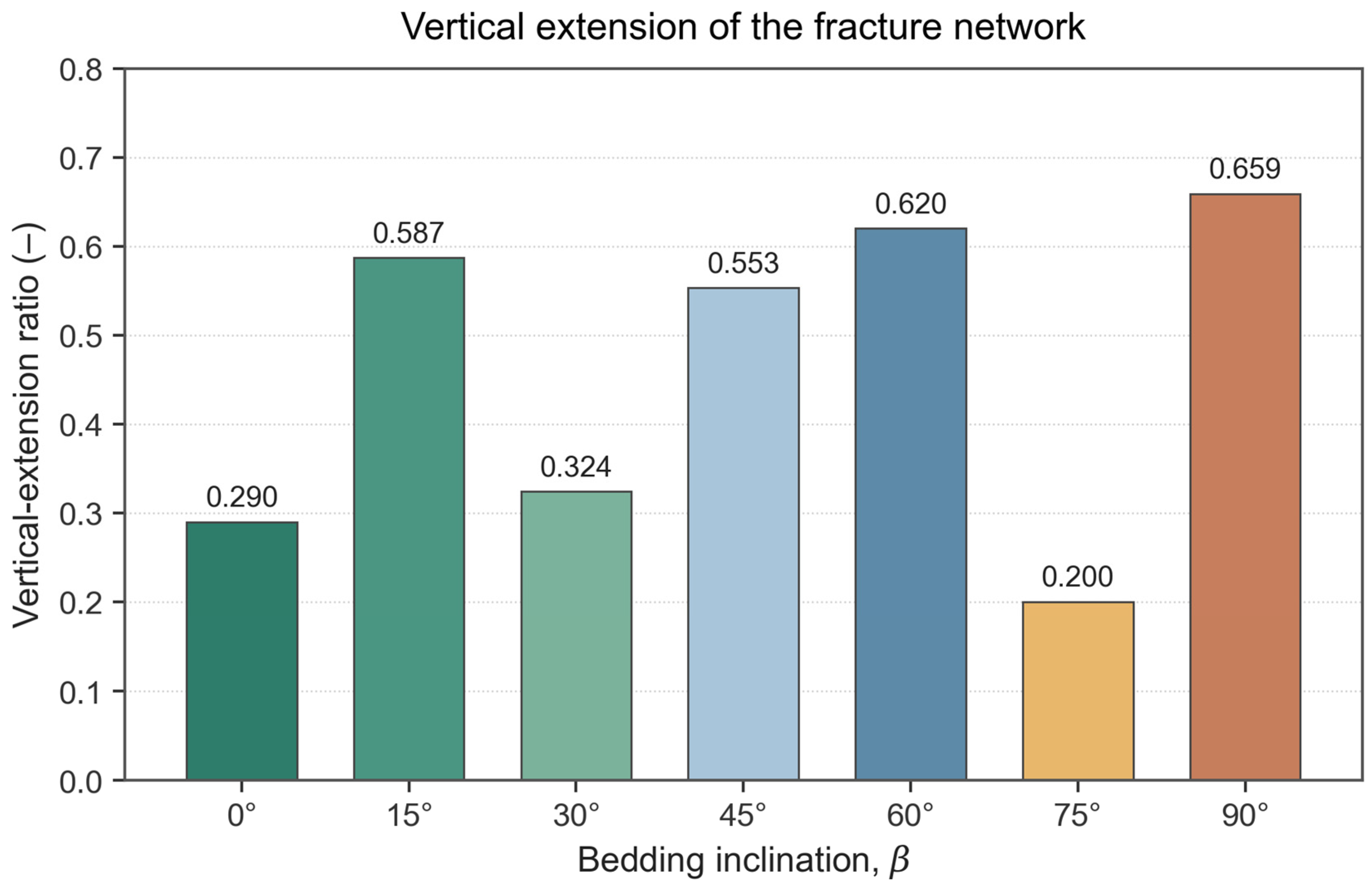
The vertical-extension ratio (Figure 11) further distinguishes two extension modes. The 90° case follows a sudden-breakthrough mode: the curve exhibits a step-like jump near 100 MPa, rising from 0.16 to 0.659, and produces a simple through-going vertical fracture with limited branching. The 45° and 60° cases follow a progressive-extension mode: the 60° case grows smoothly from the low-pressure stage to 0.620 with clear branching at each layer-crossing event, and the 45° case reaches 0.571 with similar progressive-crossing behaviour. The 15°, 30°, and 0° cases give only 0.587, 0.324, and 0.290—the network is dominated by horizontal extension and the vertical stimulation thickness is very limited.

Figure 11. Evolution of the vertical-extension ratio during fracture propagation for different bedding inclinations.

To rank the seven cases on an objective basis, four sub-scores are constructed from the peak fracturing pressure P and the three propagation indicators—lateral reach L, vertical reach V, and the geometric-mean proxy $\sqrt{LV}$ for the stimulated volume. Each sub-score is rescaled to the unit interval so that higher is always better:

$$s_1={\displaystyle \frac{P_{max}-P}{P_{max}-P_{min}}}$$

(5)

$$s_2={\displaystyle \frac{L}{L_{max}}}$$

(6)

$$s_3={\displaystyle \frac{V}{V_{max}}}$$

(7)

$$s_4={\displaystyle \frac{\sqrt{LV}}{\sqrt{L_{max}{V}_{max}}}}$$

(8)

where s1 is the initiation-efficiency score, s2 and s3 are the lateral and vertical reach scores, and s4 is the stimulated-volume proxy score. An equal-weight composite score is then computed for each case,

$$S={\displaystyle \frac{1}{4}}\left(s_1+s_2+s_3+s_4\right)$$

(9)

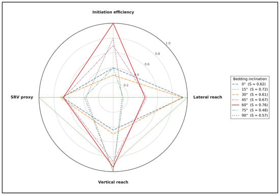
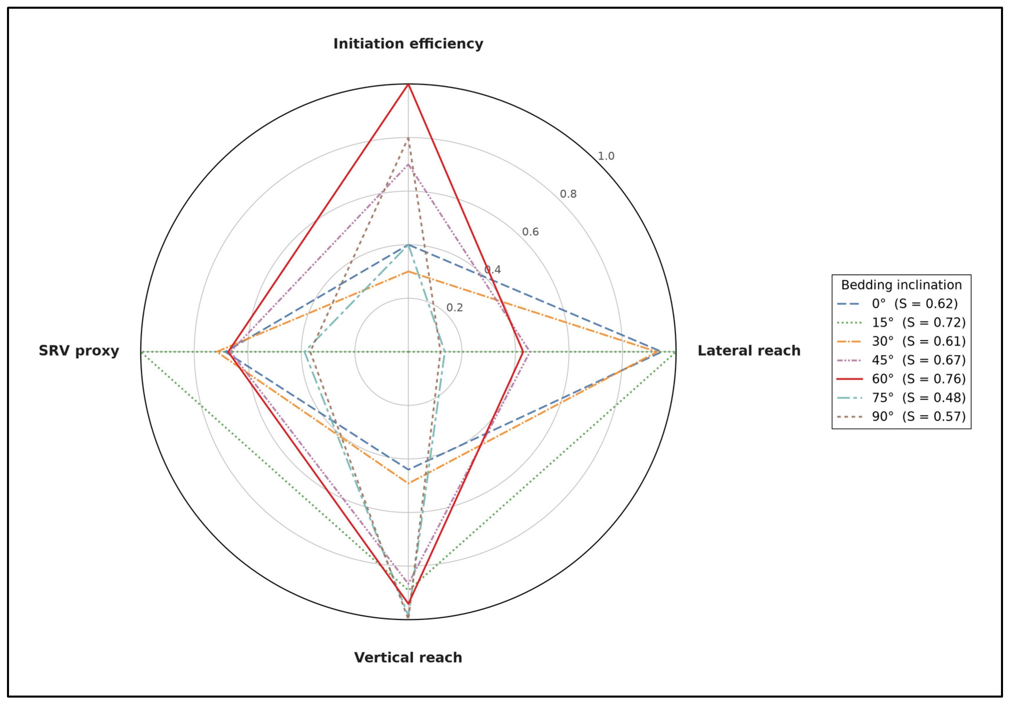
with equal weights adopted in the absence of a project-specific engineering priority; the ranking is verified to be robust to reasonable weight perturbations. The four sub-scores and the composite S are shown as a radar chart in Figure 12 and summarised in Table 7.

Figure 12. Comprehensive stimulation-score radar chart for the seven bedding inclinations. Each polygon corresponds to one bedding attitude; the four axes are the initiation efficiency (s₁), lateral reach (s₂), vertical reach (s₃), and SRV proxy (s₄), rescaled to the unit interval. The composite score S in the legend is the equal-weight mean of the four sub-scores. The 60° case (red, solid) delivers the largest and most uniform polygon, giving the highest composite score S = 0.76.

Table 7. Composite stimulation-score rubric for the seven bedding inclinations.

Angle	Initiation Efficiency S1	Lateral Reach S2	Vertical Reach S3	SRV Proxy S4	Total Score S
0°	0.40	0.95	0.44	0.68	0.62
15°	0.00	1.00	0.89	1.00	0.72
30°	0.30	0.93	0.49	0.72	0.61
45°	0.70	0.45	0.87	0.66	0.67
60°	1.00	0.43	0.94	0.67	0.76
75°	0.40	0.14	0.99	0.39	0.48
90°	0.80	0.12	1.00	0.37	0.57

Ranked by S, the seven cases fall in the order 60° (0.76) > 15° (0.72) > 45° (0.67) > 0° (0.62) > 30° (0.61) > 90° (0.57) > 75° (0.48). The 60° case leads the group because it combines the lowest initiation threshold (s₁ = 1.00), high vertical reach (s₃ = 0.94), and a mid-range but balanced lateral reach (s₂ = 0.43); its radar polygon (Figure 12, red) is the most convex, indicating the most uniform performance across the four dimensions. The 15° case is a close runner-up thanks to strong lateral reach and the highest SRV proxy, but its extreme initiation cost (s₁ = 0.00 at P = 160 MPa) makes it engineeringly less attractive. The 75° and 90° cases are penalised by very weak lateral reach (s₂ ≤ 0.14), and the 30°/0° cases are penalised by weak vertical reach (s₃ ≤ 0.49). A bedding inclination of 60° is therefore identified as the optimal target attitude for hydraulic-fracturing stimulation of the Qiongzhusi Formation shale, with 15° and 45° as the second-best options depending on whether lateral coverage or vertical crossing is prioritised.

3.2. Effect of Stress Level and Stress Difference on Fracture Network Evolution

3.2.1. Fracture-Propagation Response Under Different Stress Combinations

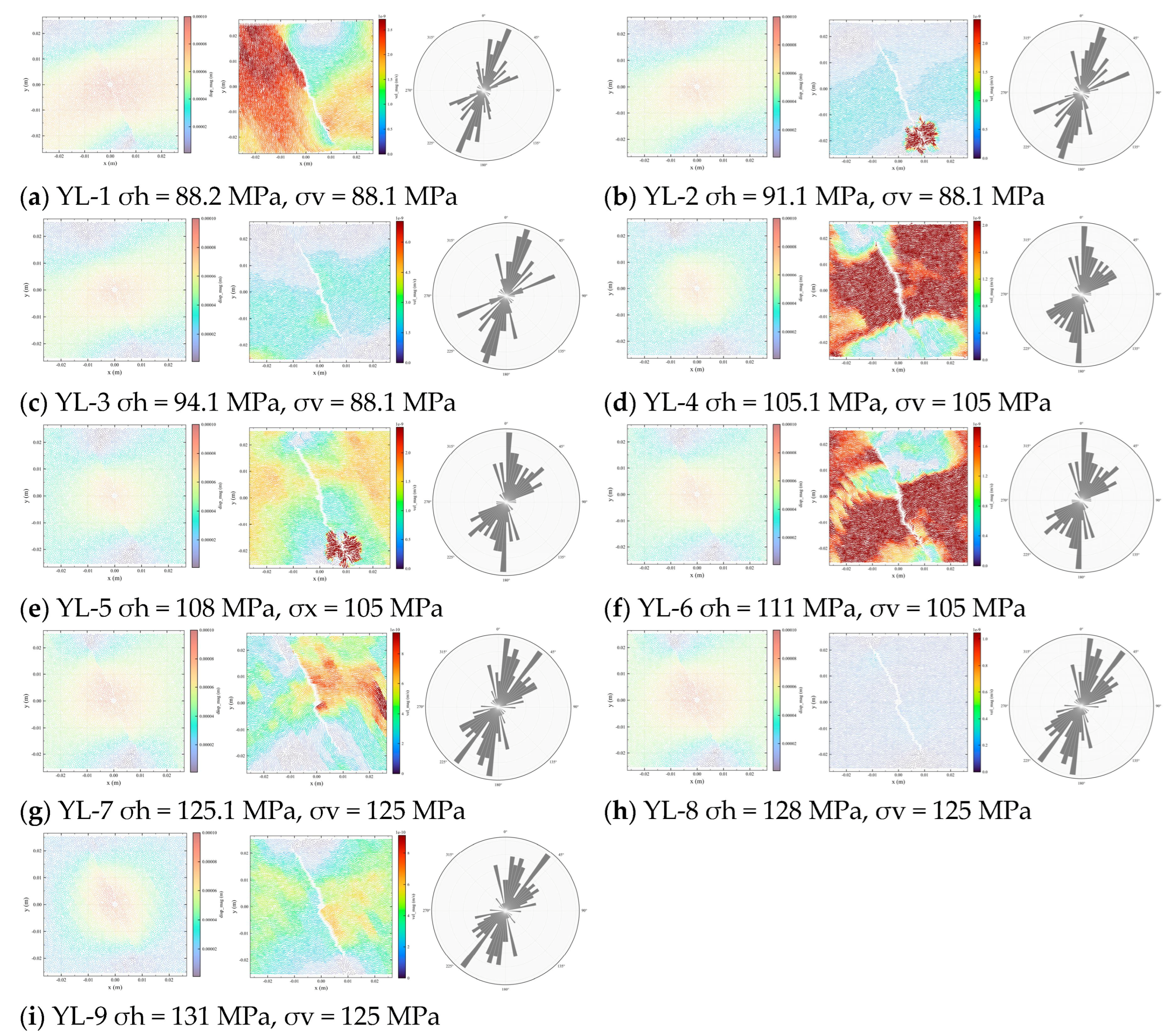
After completing the construction of the stress-sensitivity test model, the second family of parametric simulations was carried out to analyse the fracture-propagation process under the nine loading combinations YL-1 to YL-9. The present sub-section focuses on the temporal evolution of fracture propagation, the propagation direction, and the displacement-perturbation characteristics as the fracture progresses from initiation through extension to boundary crossing, in order to reveal how the stress state controls the propagation path and network geometry.

The simulation results show that when the stress difference is increased, the number of calculation timesteps required for the fracture to reach the model boundary is significantly enlarged, indicating that a larger stress difference increases the difficulty for the fracture to overcome confining constraints and to sustain propagation. Under low stress level conditions, when ${\sigma }_{\mathrm{x}}$ = 85 MPa the fracture reaches the model boundary after approximately 12,000 timesteps, and its main-fracture azimuth is oriented at approximately 22°. When ${\sigma }_{\mathrm{x}}$ is increased to 105 MPa, the number of timesteps required to reach the boundary grows to approximately 30,000, while the main azimuth remains in the vicinity of 22°. When ${\sigma }_{\mathrm{x}}$ is further increased to 125 MPa, the timesteps required to reach the boundary grow to approximately 50,000, and the main-fracture azimuth simultaneously rotates to approximately 40°. These observations reveal that as the stress level increases, the fracture propagation is subjected to stronger closure-stress constraints, the propagation rate slows down, and the propagation direction may also deflect.

From the perspective of the displacement-perturbation distribution, at low stress levels the large-displacement perturbation zone is concentrated in the central region on both sides of the fracture, indicating that early-stage fracture propagation is dominated by local opening and near-wellbore perturbation. As the stress level and stress difference increase, the displacement-perturbation zone gradually migrates from the central sides of the fracture towards the model edges, indicating that during sustained fracture propagation, the fracture is jointly constrained by the boundary stress field and the far-field principal-stress direction, where its propagation path tends to extend steadily along the direction of dominant stress. This phenomenon reflects the fact that under higher stress conditions, fracture propagation is no longer driven exclusively by the local injection pressure but is increasingly governed by the directionality of the overall stress field.

3.2.2. Effect on Fracture Geometry and Failure Mode: Cross-Case Comparison

After the fracture-propagation morphologies under the nine stress combinations have been analysed, a lateral cross-case comparison of fracture geometry parameters, failure-mode composition, pressure response, and stress-perturbation indicators is now performed to evaluate the effects of stress level and stress difference on the final geometry of the hydraulic fracture in a quantitative manner, as shown in Figure 13. Overall, the sensitivity of the final hydraulic-fracture geometry to changes in stress level is relatively weak: the geometrical scale of the fracture shows no abrupt discontinuities across the nine stress combinations. This indicates that under the present model configuration, changes in stress state manifest themselves primarily as adjustments to the propagation process, the pressure response, and the failure mode, rather than as complete transformations of the final fracture geometry.

From the perspective of the effect of stress level, as the stress level increases, the total number of fractures, the shear-to-tensile fracture ratio, and the central stress all increase. This indicates that under higher confining-pressure conditions the rock failure process is subjected to stronger compressive constraints, where fracture propagation requires a higher local stress concentration to be sustained. Simultaneously, the pressure-perturbation area follows a first-decrease-then-increase pattern, indicating that under intermediate stress levels the diffusion of injected-fluid pressure may be more strongly suppressed, whereas under high stress levels the enhanced driving force for rupture again enlarges the pressure-perturbation domain. The pressure peak follows a non-monotonic, domed pattern with a maximum near σ_h ≈ 105 MPa (cases YL-4–YL-6) and a subsequent decline at σ_h = 125 MPa, reflecting a non-linear regulation among fracture opening, pressure accumulation, and rupture release under different stress levels.

From the perspective of the effect of stress difference, as the stress difference increases, the total number of fractures and the shear-to-tensile fracture ratio both increase, indicating that enhanced stress difference strengthens the directionality of fracture propagation and promotes the proportion of shear rupture. Under large-stress-difference conditions, fractures tend to propagate more strongly along the direction of the maximum stress, and natural weak planes or local structural surfaces are more prone to shear slip under the action of differential stress, causing the fraction of shear fractures to rise. At the same time, the pressure peak shows a weak decreasing trend that is comparatively minor relative to the effect of the basal stress level, indicating that under large-stress-difference conditions, once an effective propagation channel has formed along the dominant direction, the fluid pressure is more easily relieved through fracture extension.

Figure 13. Simulated fracture-propagation patterns under the nine stress combinations YL-1–YL-9. For each case, the three panels show, from left to right, the particle-displacement field, the velocity field, and the rose diagram of fracture orientations. (a) YL-1: σ_h = 88.2 MPa, σ_v = 88.1 MPa; (b) YL-2: σ_h = 91.1 MPa, σ_v = 88.1 MPa; (c) YL-3: σ_h = 94.1 MPa, σ_v = 88.1 MPa; (d) YL-4: σ_h = 105.1 MPa, σ_v = 105 MPa; (e) YL-5: σ_h = 108 MPa, σ_x = 105 MPa; (f) YL-6: σ_h = 111 MPa, σ_v = 105 MPa; (g) YL-7: σ_h = 125.1 MPa, σ_v = 125 MPa; (h) YL-8: σ_h = 128 MPa, σ_v = 125 MPa; (i) YL-9: σ_h = 131 MPa, σ_v = 125 MPa.

Figure 13. Simulated fracture-propagation patterns under the nine stress combinations YL-1–YL-9. For each case, the three panels show, from left to right, the particle-displacement field, the velocity field, and the rose diagram of fracture orientations. (a) YL-1: σ_h = 88.2 MPa, σ_v = 88.1 MPa; (b) YL-2: σ_h = 91.1 MPa, σ_v = 88.1 MPa; (c) YL-3: σ_h = 94.1 MPa, σ_v = 88.1 MPa; (d) YL-4: σ_h = 105.1 MPa, σ_v = 105 MPa; (e) YL-5: σ_h = 108 MPa, σ_x = 105 MPa; (f) YL-6: σ_h = 111 MPa, σ_v = 105 MPa; (g) YL-7: σ_h = 125.1 MPa, σ_v = 125 MPa; (h) YL-8: σ_h = 128 MPa, σ_v = 125 MPa; (i) YL-9: σ_h = 131 MPa, σ_v = 125 MPa.

3.2.3. Evolution of Failure Mode with Confining Pressure

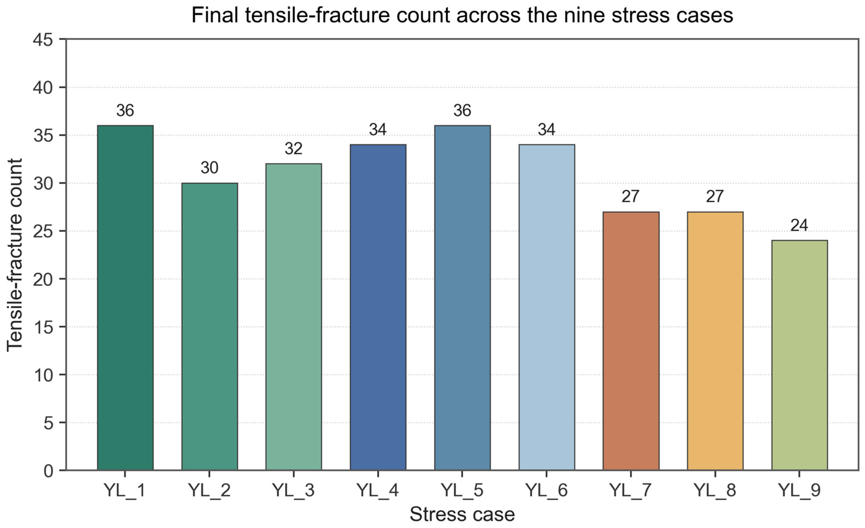
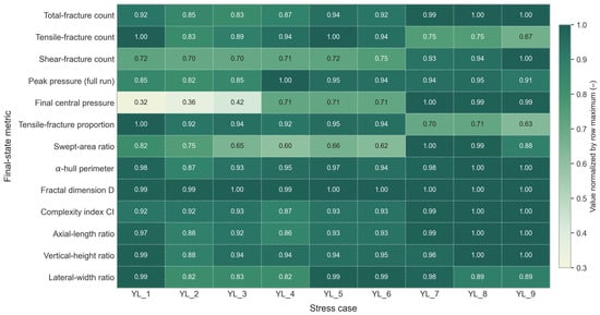
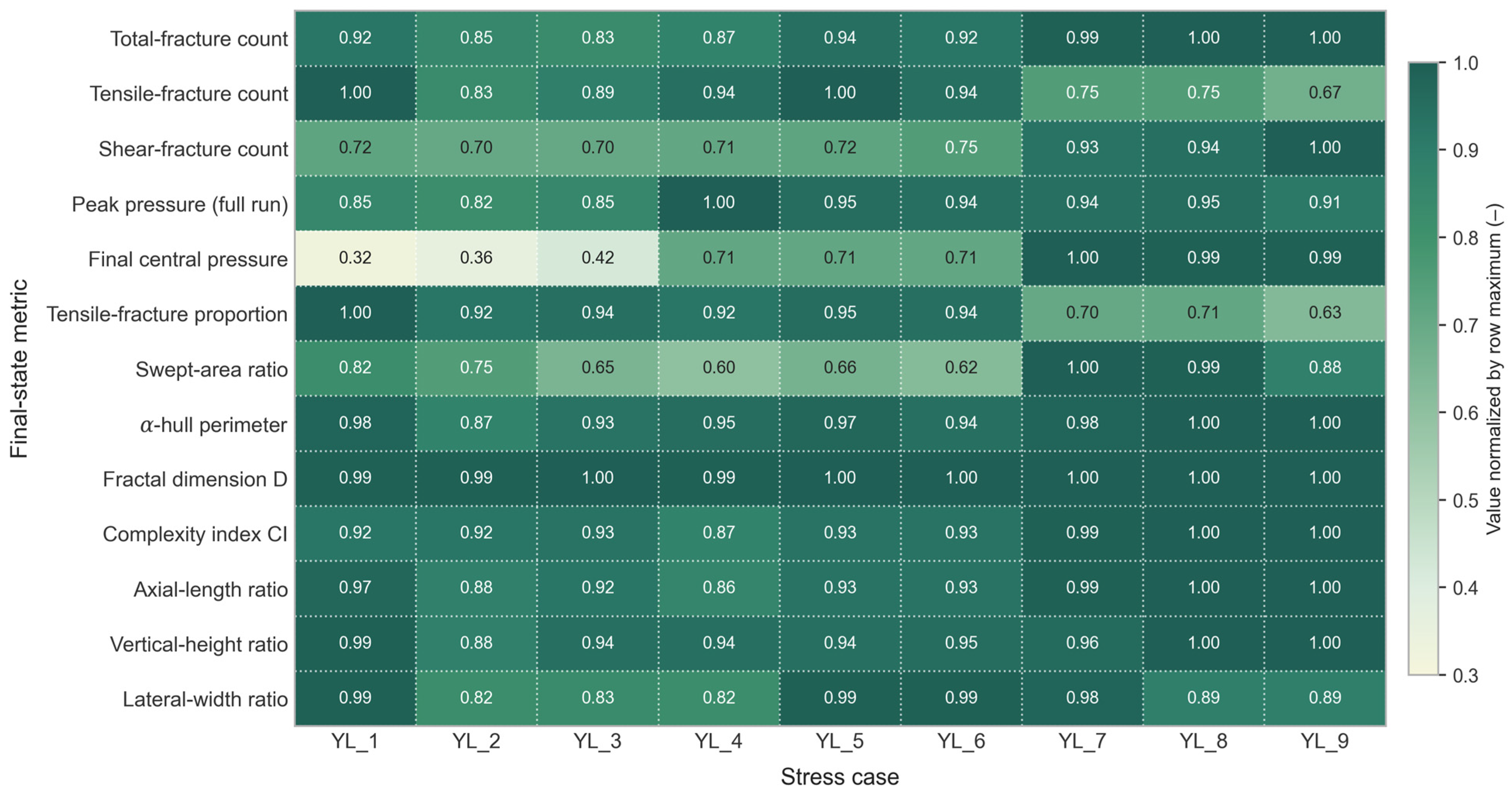
Building on the geometry and failure-mode composition of Section 3.2.2, the effect of confining pressure on the failure mechanism and on the overall stress response is now examined by tracing the evolution of the tensile–shear composition across the nine cases. The statistical results are shown in Figure 14, Figure 15, Figure 16, Figure 17.

Figure 14. Normalised final-state metrics for the nine stress combinations YL-1–YL-9, presented as a row-normalised heatmap grouped by axial stress σ_y.

Increasing confining pressure gradually shifts the failure mechanism of the Qiongzhusi Formation shale from brittle failure at low confining pressure to ductile failure at high confining pressure. When the basal horizontal stress σ_h is raised from the lowest level (88.1 MPa, effective σ_h = 0.1 MPa) to the highest level (125 MPa, effective σ_h = 37 MPa), the time required for the hydraulic fracture to reach a stable propagation stage is extended to approximately four times its original value. Over the same range, the peak pore pressure follows a domed response with its maximum near σ_h ≈ 105 MPa, and then declines by roughly 6–9% (row-normalised, Figure 14) as σ_h rises further to 125 MPa. Under high-confinement conditions the particle contacts of the rock experience stronger compaction, fracture opening is suppressed, and the propagation transitions from rapid brittle cracking to gradual progressive failure.

The failure-mode composition evolves in parallel. Under low confining pressure the fractures initiate and propagate rapidly in a tensile mode, with pronounced fracture opening and concentrated failure processes. Under high confining pressure the fracture surfaces are subjected to stronger normal compressive stresses; purely tensile opening is suppressed, and shear slip together with combined shear–tensile failure becomes dominant. The tensile-fracture proportion decreases from an initial value of 1.0 at initiation to a stable range of 0.25–0.35, i.e., approximately 65–75% of the fractures generated in the later stage are contributed by shear failure.

Taken together, the results of Section 3.2 identify the in situ stress state as an important boundary condition controlling hydraulic-fracture propagation in Qiongzhusi shale. The basal stress level primarily controls the difficulty of fracture opening, the duration of propagation, and the intensity of the pore-pressure response, whereas the vertical–horizontal stress difference further modulates the propagation direction, the shear-to-tensile fracture ratio, and the complexity of the network. As the stress level increases, propagation shifts from rapid brittle tensile splitting under low confining pressure to combined shear–tensile ductile failure under high confining pressure. As the stress difference increases, both the total number of fractures and the shear-to-tensile ratio rise, indicating that differential stress favours weak-plane slip and shear rupture but also enhances the directionality of propagation.

Figure 15. Final swept-area ratio for the nine stress cases YL-1–YL-9.

Figure 15. Final swept-area ratio for the nine stress cases YL-1–YL-9.

Figure 16. Final shear-fracture count for the nine stress cases YL-1–YL-9.

Figure 16. Final shear-fracture count for the nine stress cases YL-1–YL-9.

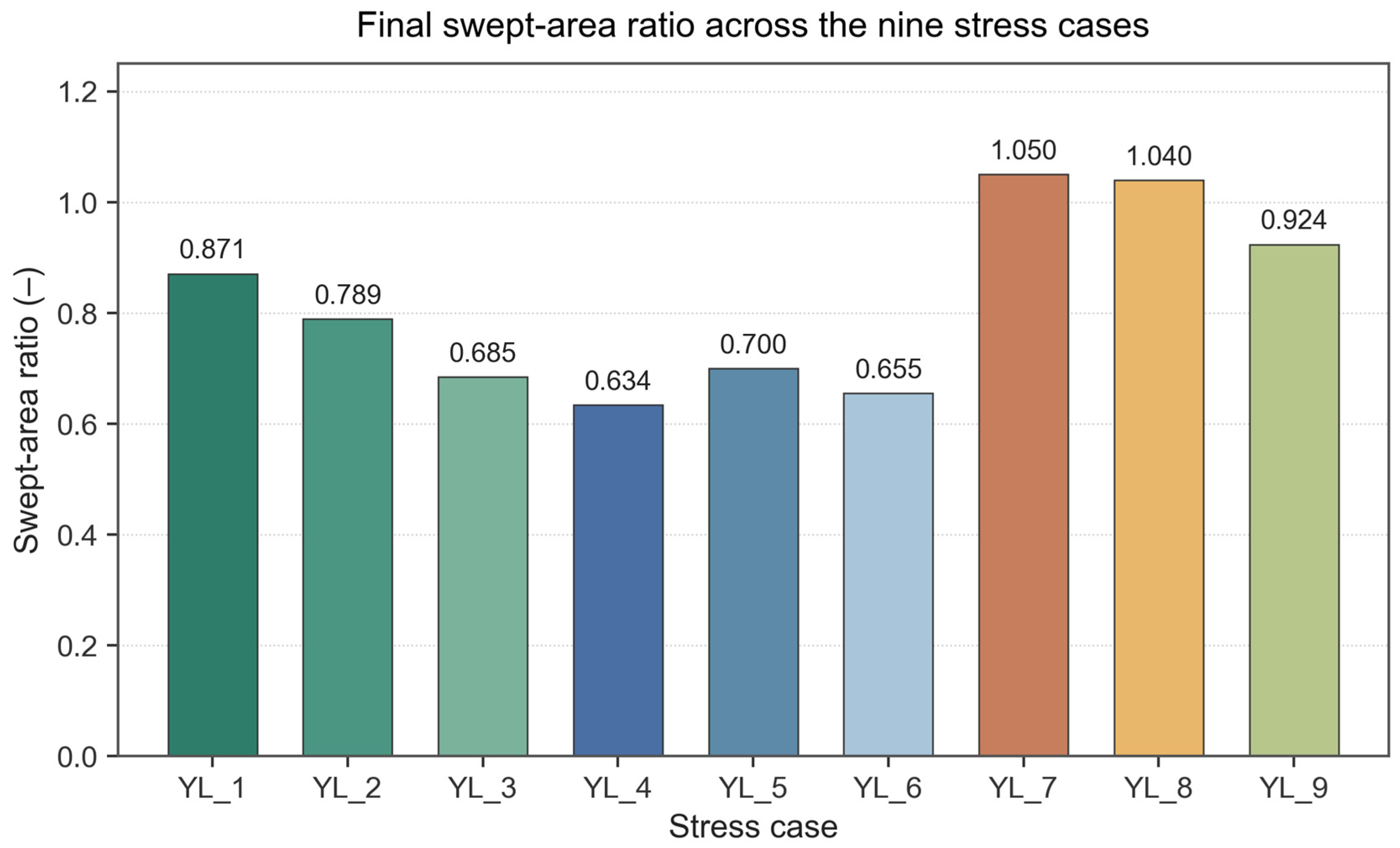
Figure 17. Final tensile-fracture count for the nine stress cases YL-1–YL-9.

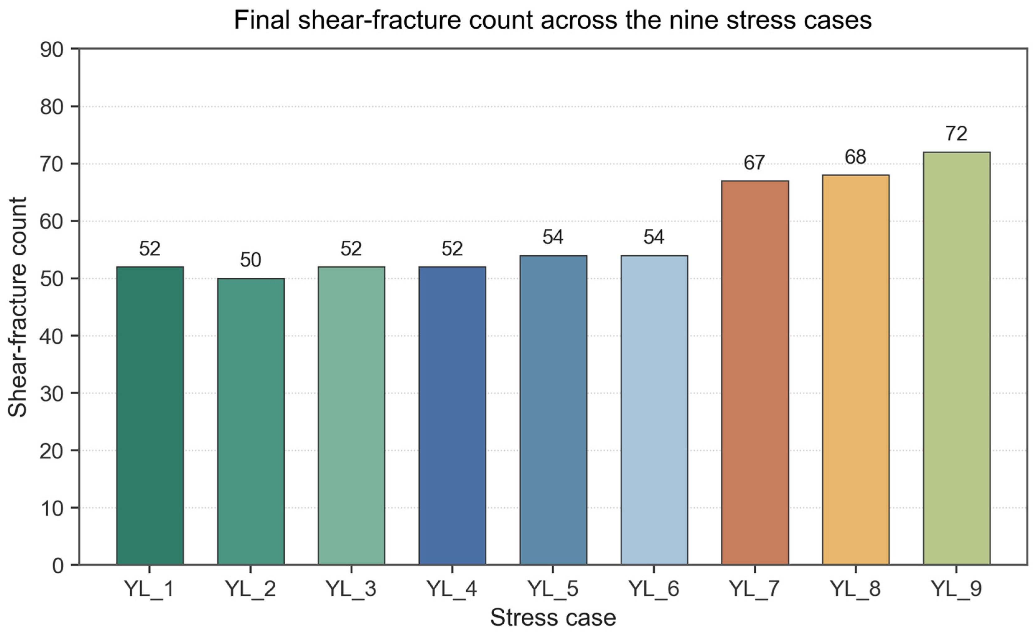
Figure 17. Final tensile-fracture count for the nine stress cases YL-1–YL-9.

3.2.4. Statistical Decomposition via Response-Surface Analysis

Section 3.2.1, Section 3.2.2 and Section 3.2.3 established, on a case-by-case basis, that both the basal horizontal stress σ_h and the vertical–horizontal stress difference σ_v − σ_h leave an imprint on the fracture network response. To resolve their individual roles more sharply, and in particular to determine which of the two dominates when their signals point in opposite directions, a quadratic response-surface model together with a two-way analysis of variance was fitted to the 3 × 3 full-factorial design of Table 6. The two coded factors are X₁ = σ_h ∈ {−1, 0, +1} corresponding to 88.1, 105, 125 MPa and X₂ = σ_v − σ_h ∈ {−1, 0, +1} corresponding to 0.1, 3, 6 MPa. Nine response variables were considered: total, shear-, and tensile-fracture counts, shear-to-tensile ratio, tensile-fracture proportion, swept-area ratio, and the row-normalised peak pressure, central pressure, and complexity index CI. The full quadratic surface, as given by Equation (10), is:

$$y=b_0+b_1{X}_1+b_2{X}_2+b_{12}{X}_1{X}_2+b_{11}{X_1}^2+b_{22}{X_2}^2$$

(10)

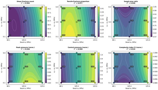
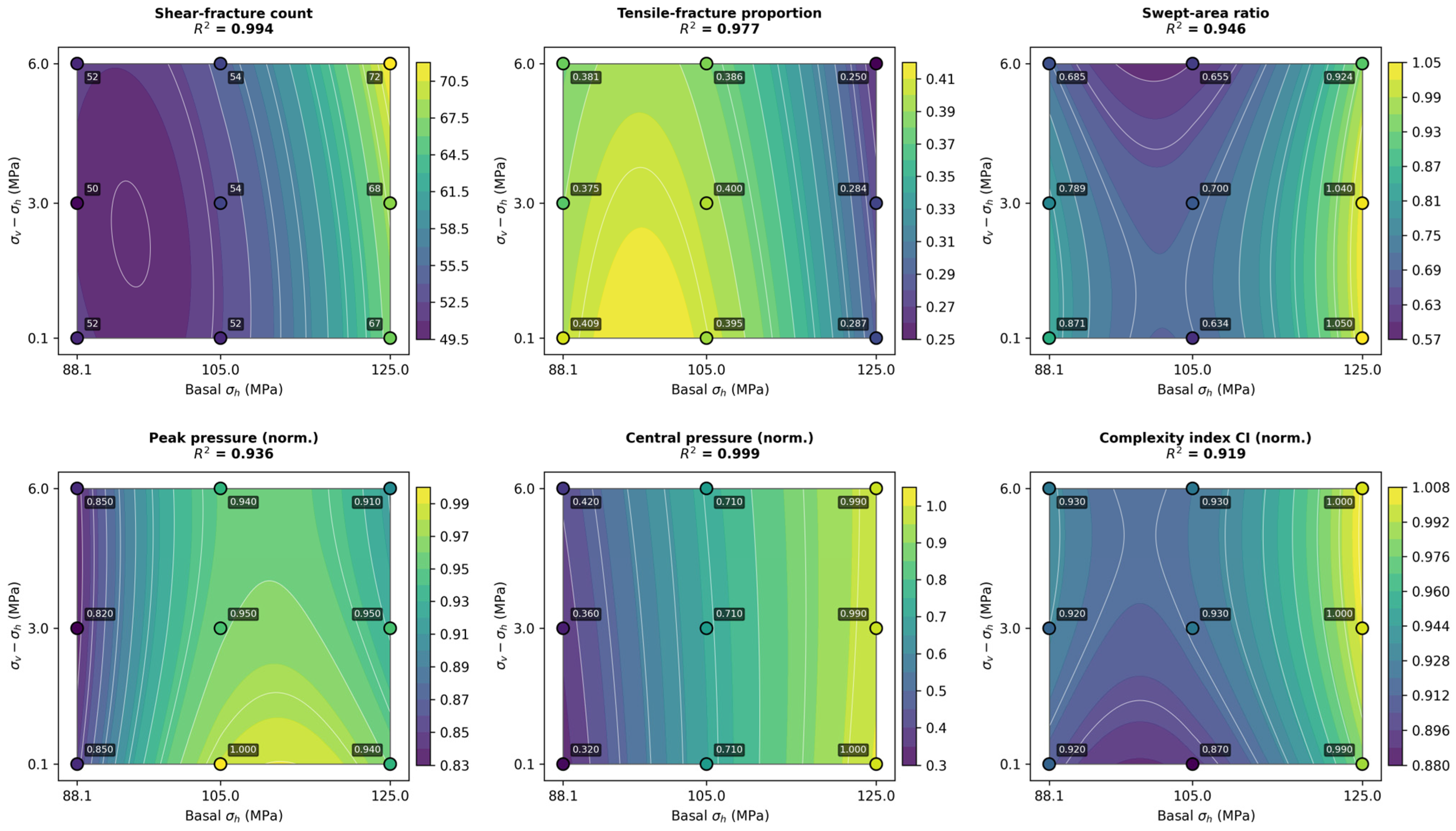
Equation (10) was fitted by ordinary least squares. Adjusted R² exceeds 0.83 for seven of the nine responses and reaches 0.997 for central pressure and 0.984 for shear count, so the surface is close to interpolation for shear and central pressure and remains a faithful description for the remaining responses (Table 8, Figure 18). The ANOVA contribution rates are summarised in Table 8.

Table 8. Analysis of variance for the response surface quadratic model.

Response Variable	Contribution of σh (%)	P(σh)	Contribution of σv − σh (%)	P(σv − σh)	Error (%)
Total fracture count	81.6	0.031	0.9	0.907	17.5
Shear-fracture count	96.7	0.0003	1.6	0.256	1.7
Tensile-fracture count	81.9	0.018	5.4	0.489	12.7
Shear-to-tensile ratio	92.5	0.0015	3.8	0.245	3.7
Tensile-fracture proportion	94.5	0.0006	3.2	0.182	2.4
Swept-area ratio	86	0.004	8.2	0.171	5.8
Peak pressure (norm.)	87.5	0.006	5.3	0.335	7.2
Central pressure (norm.)	99.1	0.00004	0.2	0.529	0.6
Complexity index CI (norm.)	83.8	0.008	8.1	0.25	8.1

Figure 18. Quadratic response surfaces of the six key fracture network and pressure responses over the 3 × 3 stress-sensitivity design. Axes are the basal horizontal stress σ_h (88.1, 105 and 125 MPa) and the differential stress σ_v − σ_h (0.1, 3 and 6 MPa); filled contours are the fitted second-order response surfaces; circles are the nine design points labelled with their simulated values, and R² is given for each fit.

The two factors influence disjoint aspects of the fracturing response. σ_h independently controls the intensity of the response: the absolute level of the central and peak fluid pressures, the tensile-fracture proportion, and the shear-to-tensile ratio all track basal stress alone (contribution of 87–99%, p ≤ 0.006), while σ_v − σ_h leaves them within noise (all p > 0.13). σ_v − σ_h, by contrast, is most visible on the spatial character of the network: for the swept-area ratio and the complexity index CI, its contribution rises to 6–8%, still below the 5% significance threshold but the largest sensitivity observed among the nine responses. A smaller vertical–horizontal difference is associated with slightly wider swept areas and marginally lower CI, consistent with the physical picture that a nearly isotropic in-plane stress state allows fluid pressure to diffuse more evenly rather than being channelled along a dominant direction.

The response along the basal-stress axis is furthermore non-monotonic: the X₁² term is significant for shear count, swept area, peak pressure, and complexity index (all p < 0.05). For shear count, swept area, and CI the curvature is upward—additional basal stress is absorbed comparatively easily at 88.1 MPa but strongly amplifies shear activation and network spread between 105 and 125 MPa. For the peak fluid pressure the surface is instead domed, with its maximum at σ_h ≈ 110 MPa; both the lowest and the highest basal levels correspond to modestly lower peak pressures than the intermediate level, in agreement with the qualitative description of Section 3.2.2.

When the two factors send signals in the same direction, the joint response is well approximated by the sum of their individual contributions. A simultaneous rise in σ_h and σ_v − σ_h from case YL-1 to case YL-9 produces a monotonic evolution across all indicators: the total fracture count grows from 88 to 96; the shear-to-tensile ratio rises from 1.44 to 3.00, and the tensile-fracture proportion falls from 0.41 to 0.25. When the two factors point in opposite directions, however, the response is dictated almost exclusively by σ_h. Comparing case YL-3 (σ_h = 88.1 MPa, σ_v − σ_h = 6 MPa) with case YL-7 (σ_h = 125 MPa, σ_v − σ_h = 0.1 MPa) shows that the case with the higher basal stress delivers the larger total count (94 vs. 84), a substantially higher shear-to-tensile ratio (2.48 vs. 1.63), a lower tensile-fracture proportion (0.29 vs. 0.38), and a larger swept area (1.05 vs. 0.685), even though its vertical–horizontal stress difference is the lowest of the design. The only response for which the two factors show a statistically detectable interaction is the central pressure (b₁₂ = −0.028, p = 0.037): in the low-σ_h, high-(σ_v − σ_h) corner the surface bends downward relative to the additive prediction, but the magnitude of this deviation is only a few percent of the mean and does not overturn the dominance of the basal stress.

Taken together, these results assign σ_h to the pressure and failure-mode aspects of the response, and σ_v − σ_h to a secondary modulation of the network’s spatial extent. When the two axes carry conflicting signals, the σ_h effect prevails. This picture converts the case-by-case observations of Section 3.2.1, Section 3.2.2 and Section 3.2.3 into a compact, statistically supported framework, and forms the basis for the engineering considerations discussed in Section 4.

4. Discussion

Hydraulic-fracture propagation in the Qiongzhusi Formation shale is not governed by any single factor. Bedding weak planes largely reshape the propagation path and the stimulated-volume potential, while the in situ stress boundary influences the far-field propagation direction and the sustainability of propagation; the two act in parallel rather than substitutively. Matrix heterogeneity, although not systematically varied here, provides the material context in which they operate: stiff clusters develop local stress concentrations, whereas low-strength contacts and locations adjacent to bedding surfaces are more prone to tensile splitting or shear slip.

Bedding weak planes exert a dual effect. When their development is moderate, they act as inducers of branching, increasing connectivity and expanding the effective stimulated zone [28,29]. When they are over-developed, or when their attitude aligns closely with the stress state, injected fluid energy is preferentially consumed in slip along a single weak-plane family, vertical height growth is constrained, and network complexity is reduced [30,31]. Weak planes are therefore not universally favourable: their effect depends on the joint configuration of attitude, density, and stress environment. This provides a mechanistic explanation for the field observation that some Qiongzhusi sub-layers with well-developed bedding produce disappointing stimulation outcomes, and is consistent with laboratory interaction experiments between induced and pre-existing fractures [32].

These bedding-controlled behaviours find support in independent results obtained by other methods. In the true-triaxial experiments of Zhang et al. on Lushan shale [13], the interplay of bedding inclination with the applied stress state governed whether the fracture crossed or was deflected along the beds, which corresponds to the crossing–deflection transition observed here between the intermediate and high-angle cases. The criterion of Renshaw and Pollard [11] indicates that crossing requires the fluid pressure to overcome both the normal stress acting on the interface and its tensile strength, offering an explanation for the elevated fracturing pressures obtained at low bedding angles, where the beds are oriented unfavourably for opening and the fracture must cross them. The numerical results of Zou et al. [22] similarly show that bedding planes redistribute the injected energy between along-bed and across-bed propagation and thereby influence the balance between lateral and vertical extension, which is in line with the opposing trends of the two extension ratios reported in Section 3.1.2. The finite-discrete element simulations of Wang et al. on lamellar shales [33] are particularly relevant here: they report that the breakdown pressure reaches its maximum at a bedding inclination of 0° and its minimum at 60°, and that inclined bedding favours steering- and capture-type fractures while bedding aligned with the minimum principal stress favours layer-penetrating and bifurcated growth. Both observations correspond closely to the U-shaped pressure–inclination relation and the progressive branching behaviour identified here at 60°. That two rather different numerical frameworks—a bonded-particle model and a finite-discrete element model—arriving at a consistent picture lends additional confidence to the 60° optimum reported in this study.

As the basal stress level rises, the fluid pressure required for fracture opening follows a non-monotonic, domed response with a maximum near σ_h ≈ 110 Mpa; propagation lasts longer, and the failure mechanism shifts from rapid tensile splitting to combined shear–tensile rupture. The response-surface analysis of Section 3.2.4 sharpens this picture: σ_h accounts for 82–99% of the variance of every response and is significant throughout, whereas σ_v − σ_h contributes at most 8.2% and reaches significance for none. Within the field-stress envelope of the Qiongzhusi Formation, the stress difference therefore refines the directionality of propagation without altering the pattern set by the basal stress level. Taken with the bedding results, this suggests a division of labour between the two controls: bedding attitude shapes the geometry of the emerging network, while the stress state governs its kinematics—the duration of propagation, the pressure required to sustain it, and the balance between tensile and shear failure.

Three implications follow for practice. Target-interval screening should combine mineral brittleness assessment with bedding-attitude evaluation, favouring inclinations in the 45–60° range, which return the two highest composite scores of the seven attitudes examined. Treatment energy should be scaled with σ_h rather than with the stress difference: over the interval from 88.1 to 125 MPa the propagation time lengthens roughly fourfold, so sub-layers in the upper part of this range require correspondingly greater injected energy to sustain propagation. In intervals with well-developed bedding, natural weak planes should be exploited actively as network-inducing elements, with the design aimed at maximising the number activated.

Several limitations should be acknowledged. The model is two-dimensional and cannot reproduce three-dimensional height evolution or multi-stage interaction along a horizontal well. The fluid–solid coupling treats the fluid as Newtonian with a single viscosity and omits proppant transport, matrix leakoff, and temperature dependence, so the simulations represent the fracture-mechanics response rather than the full engineering behaviour of a treatment. Calibration is anchored to a single core from 4601.76 m; broader calibration across samples and depths would improve generalisability. Mineral heterogeneity is represented in lumped form through spatial variation in the parallel-bond parameters rather than as an explicit mineralogical map. Finally, the stress sensitivity was established at a single bedding attitude, so the reported contribution rates apply strictly to the 60° configuration; a full cross-comparison over low-, intermediate-, and high-angle beddings under the same stress design is planned for subsequent work.

5. Conclusions

A DEM hydraulic-fracturing model coupling bedding weak planes and in situ stress was calibrated against a triaxial-compression test on a Qiongzhusi core from a 4601.76 m depth, and used to examine how these two controls together shape the resulting fracture network. The following conclusions summarise the main observations from the bedding-angle and stress-combination sensitivity analyses:

(1)

Bedding weak planes govern network geometry. Low-angle bedding (0–30°) favours lateral extension (ratios of 0.63–0.68) but limits vertical connectivity; high-angle bedding (75–90°) promotes vertical breakthrough while restricting lateral reach. Ranked by a composite stimulation score built from four normalised sub-scores, a 60° inclination is the optimum (S = 0.76), ahead of 15° (0.72) and 45° (0.67), combining the lowest fracturing pressure (110 MPa), vertical- and lateral-extension ratios of 0.62 and 0.29, and progressive branching.

(2)

In situ stress mainly modulates the propagation kinematics rather than the final planar extent. Raising σ_h from 88.1 to 125 MPa slows propagation approximately fourfold and shifts the failure mode from tensile splitting to shear–tensile ductile rupture, with the tensile-fracture proportion falling from 1.0 to 0.25–0.35. A two-way analysis of variance over the nine stress cases attributes 82–99% of the variance of every response to σ_h (p ≤ 0.031), while σ_v − σ_h contributes at most 8.2% and does not reach significance for any response (p > 0.17). Within the field-stress envelope of the Qiongzhusi Formation, the two controls therefore combine additively rather than multiplicatively, with the basal stress level setting the response and the stress difference refining its directionality.

(3)

For engineering practice, target-interval selection should combine mineral brittleness with bedding inclinations of 45–60°, which return the two highest composite stimulation scores of the seven attitudes examined. Because the basal stress level rather than the stress difference governs the response, treatment energy should be scaled with σ_h: over the interval from 88.1 to 125 MPa the propagation time lengthens roughly fourfold and the shear-fracture count rises from 52 to 72, so intervals in the upper part of this range require correspondingly greater injected energy to sustain propagation. In bedding-rich intervals, natural weak-plane branching should be exploited as the primary network-inducing mechanism.

References

- Zou, C.; Dong, D.; Wang, Y.; Li, X.; Huang, J.; Wang, S.; Ma, X.; Cheng, K.; Liu, D. Shale gas in China: Characteristics, challenges and prospects (I). Pet. Explor. Dev. 2015, 42, 689–701. [Google Scholar] [CrossRef] [Scilit]
- Ma, X.; Xie, J. The progress and prospects of shale gas exploration and development in southern Sichuan Basin, SW China. Pet. Explor. Dev. 2018, 45, 172–182. [Google Scholar] [CrossRef] [Scilit]
- Wang, H.; Liu, Y.; Dong, D.; Zhao, Q.; Du, D. Scientific issues on effective development of marine shale gas in southern China. Pet. Explor. Dev. 2013, 40, 615–620. [Google Scholar] [CrossRef] [Scilit]
- Liu, Y.W. Some frontier mechanics problems in shale gas production. Adv. Mech. 2019, 49, 222–248. [Google Scholar] [CrossRef]
- Yuan, J.L.; Deng, J.G.; Zhang, D.Y.; Li, D.H.; Yan, W.; Chen, C.G.; Chen, L.J.; Chen, Z.J. Fracability evaluation of shale gas reservoirs. Acta Pet. Sin. 2013, 34, 523–527. [Google Scholar] [CrossRef]
- Tang, J.; Li, J.; Zhang, Z.; Fan, Y.; Jiang, W.; Meng, S.; Zhao, X. Differential impacts of multi-scale natural fractures on hydraulic fracture network formation. Earth-Sci. Rev. 2026, 272, 105315. [Google Scholar] [CrossRef] [Scilit]
- Wang, H.Y.; Zhou, S.W.; Liu, D.X.; Jiao, P.; Liu, H. Advances and prospects of key experimental techniques for shale gas geological evaluation. Nat. Gas Ind. 2020, 40, 1–17. [Google Scholar] [CrossRef]
- Gale, J.F.W.; Laubach, S.E.; Olson, J.E.; Eichhubl, P.; Fall, A. Natural fractures in shale: A review and new observations. AAPG Bull. 2014, 98, 2165–2216. [Google Scholar] [CrossRef] [Scilit]
- Sone, H.; Zoback, M.D. Mechanical properties of shale-gas reservoir rocks. Part 1: Static and dynamic elastic properties and anisotropy. Geophysics 2013, 78, D381–D392. [Google Scholar] [CrossRef] [Scilit]
- Rickman, R.; Mullen, M.J.; Petre, J.E.; Grieser, W.V.; Kundert, D. A practical use of shale petrophysics for stimulation design optimization: All shale plays are not clones of the Barnett Shale. In SPE Annual Technical Conference and Exhibition; SPE: Denver, CO, USA, 2008. [Google Scholar] [CrossRef] [Scilit]
- Renshaw, C.E.; Pollard, D.D. An experimentally verified criterion for propagation across unbounded frictional interfaces in brittle, linear elastic materials. Int. J. Rock Mech. Min. Sci. Geomech. Abstr. 1995, 32, 237–249. [Google Scholar] [CrossRef] [Scilit]
- Li, J.; Xu, J.; Zhang, H.; Yang, W.; Tan, Y.; Zhang, F.; Meng, L.; Zang, Y.; Miao, S.; Guo, C.; et al. High seismic velocity structures control moderate to strong induced earthquake behaviors by shale gas development. Commun. Earth Environ. 2023, 4, 188. [Google Scholar] [CrossRef] [Scilit]
- Zhang, Y.F.; Long, A.F.; Zhao, Y.; Zang, A.; Wang, C.L. Mutual impact of true triaxial stress, borehole orientation and bedding inclination on laboratory hydraulic fracturing of Lushan shale. J. Rock Mech. Geotech. Eng. 2023, 15, 3131–3147. [Google Scholar] [CrossRef] [Scilit]
- Zoback, M.D.; Kohli, A.H.; Das, I.; McClure, M. The importance of slow slip on faults during hydraulic fracturing stimulation of shale gas reservoirs. In SPE Americas Unconventional Resources Conference; SPE: Pittsburgh, PA, USA, 2012. [Google Scholar] [CrossRef] [Scilit]
- Zhang, Z.; Tang, J.; Zhang, J.; Meng, S.; Li, J. Modeling of scale-dependent perforation geometrical fracture growth in naturally layered media. Eng. Geol. 2024, 336, 107499. [Google Scholar] [CrossRef] [Scilit]
- Cundall, P.A.; Strack, O.D.L. A discrete numerical model for granular assemblies. Géotechnique 1979, 29, 47–65. [Google Scholar] [CrossRef] [Scilit]
- Potyondy, D.O.; Cundall, P.A. A bonded-particle model for rock. Int. J. Rock Mech. Min. Sci. 2004, 41, 1329–1364. [Google Scholar] [CrossRef] [Scilit]
- Lisjak, A.; Grasselli, G. A review of discrete modeling techniques for fracturing processes in discontinuous rock masses. J. Rock Mech. Geotech. Eng. 2014, 6, 301–314. [Google Scholar] [CrossRef] [Scilit]
- Hyman, J.D.; Karra, S.; Makedonska, N.; Gable, C.W.; Painter, S.L.; Viswanathan, H.S. dfnWorks: A discrete fracture network framework for modeling subsurface flow and transport. Comput. Geosci. 2015, 84, 10–19. [Google Scholar] [CrossRef] [Scilit]
- Hyman, J.D.; Jiménez-Martínez, J.; Viswanathan, H.S.; Carey, J.W.; Porter, M.L. Understanding hydraulic fracturing: A multi-scale problem. Philos. Trans. R. Soc. A 2016, 374, 20150426. [Google Scholar] [CrossRef] [Scilit] [PubMed]
- Detournay, E. Mechanics of hydraulic fractures. Annu. Rev. Fluid Mech. 2016, 48, 311–339. [Google Scholar] [CrossRef] [Scilit]
- Zou, Y.; Ma, X.; Zhang, S.; Zhou, T.; Li, H. Numerical investigation into the influence of bedding plane on hydraulic fracture network propagation in shale formations. Rock Mech. Rock Eng. 2016, 49, 3597–3614. [Google Scholar] [CrossRef] [Scilit]
- Nagel, N.B.; Sanchez-Nagel, M.A.; Zhang, F.; Garcia, X.; Lee, B. Coupled numerical evaluations of the geomechanical interactions between a hydraulic fracture stimulation and a natural fracture system in shale formations. Rock Mech. Rock Eng. 2013, 46, 581–609. [Google Scholar] [CrossRef] [Scilit]
- Guo, J.; Luo, B.; Lu, C.; Lai, J.; Ren, J. Numerical investigation of hydraulic fracture propagation in a layered reservoir using the cohesive zone method. Eng. Fract. Mech. 2017, 186, 195–207. [Google Scholar] [CrossRef] [Scilit]
- Yoon, J.S.; Zang, A.; Stephansson, O. Numerical investigation on optimized stimulation of intact and naturally fractured deep geothermal reservoirs using hydro-mechanical coupled discrete particles joints model. Geothermics 2014, 52, 165–184. [Google Scholar] [CrossRef] [Scilit]
- Zhao, X.; Jin, F.; Liu, X.; Zhang, Z.; Cong, Z.; Li, Z.; Tang, J. Numerical study of fracture dynamics in different shale fabric facies by integrating machine learning and 3-D lattice method: A case from Cangdong Sag, Bohai Bay Basin, China. J. Pet. Sci. Eng. 2022, 218, 110861. [Google Scholar] [CrossRef] [Scilit]
- Thomsen, L. Weak elastic anisotropy. Geophysics 1986, 51, 1954–1966. [Google Scholar] [CrossRef] [Scilit]
- Guo, T.; Zhang, S.; Ge, H.; Wang, X.; Lei, X.; Xiao, B. A new method for evaluation of fracture network formation capacity of rock. Fuel 2015, 140, 778–787. [Google Scholar] [CrossRef] [Scilit]
- Weng, X.; Kresse, O.; Cohen, C.; Wu, R.; Gu, H. Modeling of hydraulic-fracture-network propagation in a naturally fractured formation. SPE Prod. Oper. 2011, 26, 368–380. [Google Scholar] [CrossRef] [Scilit]
- Liu, Z.P.; Feng, Q.; Wang, Y.X.; Wang, H.; Zou, L.Q.; Tang, J.Z. Fracture Height Prediction Model Considering Bedding Layer Effect and Construction Optimization Approach for Weiyuan Shale Gas Reservoirs. Well Log. Technol. 2022, 46, 114–121. [Google Scholar] [CrossRef]
- Jie, Z.J.; Zhang, M.; Sun, C.; Liu, H.G.; Chen, X.; Zhang, Z.; Tang, J.Z. Integrated Reservoir Engineering-Geological Evaluation of Fracability and Optimization of Hydraulic Fracture Propagation. Well Log. Technol. 2025, 49, 929–941. [Google Scholar] [CrossRef]
- Blanton, T.L. An experimental study of interaction between hydraulically induced and pre-existing fractures. In SPE Unconventional Gas Recovery Symposium; SPE-10847-MS; SPE: Pittsburgh, PA, USA, 1982. [Google Scholar] [CrossRef]
- Wang, M.; Gan, Q.; Wang, T.; Ma, Y.; Yan, C.; Benson, P.; Wang, X.; Elsworth, D. Propagation and complex morphology of hydraulic fractures in lamellar shales based on finite-discrete element modeling. Geomech. Geophys. Geo-Energy Geo-Resour. 2024, 10, 71. [Google Scholar] [CrossRef] [Scilit]
Disclaimer/Publisher’s Note: The statements, opinions and data contained in all publications are solely those of the individual author(s) and contributor(s) and not of MDPI and/or the editor(s). MDPI and/or the editor(s) disclaim responsibility for any injury to people or property resulting from any ideas, methods, instructions or products referred to in the content. |
© 2026 by the authors. Licensee MDPI, Basel, Switzerland. This article is an open access article distributed under the terms and conditions of the Creative Commons Attribution (CC BY) license.