Hydro-Mechanical Coupled FDEM Modeling of Multi-Cluster Hydraulic Fracture Propagation and Interaction in Shale Reservoirs

Abstract

Competition among hydraulic fractures can redistribute growth between clusters without producing a comparable increase in total fracture length. We examine this distinction using a two-dimensional hydro-mechanical finite–discrete element method (FDEM) formulation and the available three-cluster results. The formulation accounts for poroelastic deformation, matrix and fracture flow, cohesive damage and post-failure contact. At five reported times, fracture half-length and maximum aperture agree with the tabulated KGD benchmark within 3%, with mean absolute percentage errors of 1.91% and 2.00%, respectively. Increasing cluster spacing from 5 to 20 m increases middle-fracture length from 18.5 to 39.8 m and its share of the three-fracture total from 11.87% to 24.43%. In contrast, total length increases by only 4.6%. A dimensionless length uniformity index rises from 0.828 to 0.965, demonstrating that the principal spacing response is a redistribution of growth. Increasing the reported injection rate from 6 to 12 m³/min increases maximum aperture from 1.4 to 3.2 mm. Stress-difference and viscosity cases provide additional qualitative evidence of changes in fracture morphology. The results support comparative parameter screening, while the limited benchmark, unresolved implementation details and absence of discretization studies preclude a field-optimum or mesh-independent branching claim.

1. Introduction

Hydraulic fracturing creates flow paths in low-permeability reservoirs, but neighboring fractures can interact and grow unevenly. Microseismic observations in the Barnett Shale illustrate the complexity and variability of hydraulic-fracture development [1,2,3]. Numerical studies of simultaneous multiple fractures show that fracture interaction and in situ stress affect propagation geometry [4,5]. These observations motivate examining how treatment parameters influence the distribution of growth among clusters.

Classical hydraulic-fracture models provide idealized benchmarks for coupled opening and propagation; the KGD family is represented by the formulation of Geertsma and de Klerk [6,7,8]. Such benchmarks test selected length and aperture predictions, but agreement with a single planar-fracture solution does not establish accuracy for branching, fracture contact or multi-cluster competition [9,10]. FDEM combines deformable solid elements with damageable interfaces and contact, providing a framework for investigating these discontinuous processes [11].

Hydro-mechanically coupled FDEM models have already been applied to hydraulic fracturing. AbuAisha et al. [12] investigated near-wellbore propagation in homogeneous and fractured formations and showed that pre-existing joints and stress gradients affect fracture development. Yan and Jiao [13] coupled pore seepage with deformation and fracture in a two-dimensional FDEM formulation. Most directly, Liu et al. [14,15,16] coupled an FDEM solver with fracture fluid flow to study simultaneous multiple-fracture propagation and interaction. Three-dimensional hydro-mechanical FDEM developments provide a route to resolving geometry outside a two-dimensional section [17,18,19,20]. Thus, hydro-mechanical coupling and multiple-fracture simulation are established capabilities rather than new concepts introduced here.

Against this background, we investigate how horizontal stress difference, cluster spacing, injection rate and viscosity affect three-cluster fracture growth within a common two-dimensional framework. The contribution is to separate growth uniformity from total fracture length using explicitly defined indicators and to distinguish quantitative comparisons from morphology-based interpretations. The study builds on established hydro-mechanical FDEMs [21,22,23] and does not claim that coupling or multi-fracture simulation is a new numerical principle. Its conclusions concern the reported parameter cases rather than a universal spacing criterion or field treatment optimum.

Section 2 presents the governing equations and their interpretation. Section 3 reports the KGD comparison, single-factor cases and combined schedules. Section 4 discusses quantitative indicators, evidence limits and the modeling assumptions. Section 5 summarizes the supported findings.

2. Materials and Methods

2.1. Modeling Assumptions

A coupled hydro-mechanical FDEM framework is established to simulate hydraulic-fracture initiation and propagation in saturated shale. The following assumptions are introduced to retain the dominant physical processes while maintaining computational tractability:

(1)

The intact rock matrix is simplified as a fully saturated linear elastic porous medium, and fluid migration within internal micropores complies with the classical Darcy seepage theory.

(2)

Propagating hydraulic fractures are idealized as smooth parallel-plate flow channels, where low-Reynolds laminar transport of injected fracturing fluid follows the standard cubic flow law.

(3)

Rock deformation generated during hydraulic fracturing is categorized as infinitesimal strain deformation, and the initiation and progressive expansion of fractures are governed by the irreversible damage evolution criterion of the cohesive zone model.

(4)

The fracturing fluid adopted in the simulation is defined as an incompressible Newtonian fluid, and fluid percolation from fracture surfaces toward the surrounding rock matrix is incorporated into the fluid mass conservation equation.

(5)

A bidirectional fluid–solid coupling algorithm is developed based on Biot poroelastic theory, and an explicit time-stepping integration scheme is utilized for iterative dynamic solution of the multi-field coupled system.

The two-dimensional section resolves in-plane propagation and interaction for a fixed, represented out-of-plane extent. It provides a controlled geometric approximation for comparing clusters but cannot resolve fracture height or a three-dimensional stimulated volume. For a volumetric injection rate Q distributed over effective height H, the corresponding rate per unit height is q₂D = Q/H. If Q is a stage-total rate, it equals the sum of the cluster rates. Equal partitioning cannot be assumed when a shared wellbore pressure or perforation resistance controls allocation. Accordingly, the reported volumetric-rate labels are retained as case identifiers rather than interpreted as height-independent field design values.

2.2. Solid Mechanical Governing Equations

The FDEM numerical technique discretizes fractured rock media into continuous finite element units to characterize matrix deformation responses. Zero-thickness cohesive interface units are embedded at the boundaries of adjacent rock blocks to capture the whole process of hydraulic fracture initiation and progressive expansion. Meanwhile, discrete element contact mechanics are coupled to quantify the discontinuous mechanical characteristics of fractured rock, including interface extrusion, relative sliding and post-failure block displacement.

2.2.1. Dynamic Equilibrium Equation of Solid Medium

In accordance with Newton’s second law of motion, a global dynamic equilibrium formula considering structural damping is constructed to describe the transient mechanical response of rock mass nodes under fracturing disturbance.

$$\begin{array}{c}\mathit{M}\ddot{\mathit{u}}+\mathit{C}\dot{\mathit{u}}={\mathit{F}}_{\mathrm{total}}\end{array}$$

(1)

where M denotes the nodal lumped mass matrix, C represents the global damping matrix of the rock structural system, and $\ddot{\mathit{u}}$, $\dot{\mathit{u}}$, u refer to nodal acceleration, velocity and displacement vectors, respectively.

The total external load acting on rock blocks can be decomposed into five independent mechanical components:

$$\begin{array}{c}{\mathit{F}}_{\mathrm{total}}={\mathit{F}}_{\mathrm{el}}+{\mathit{F}}_{\mathrm{co}}+{\mathit{F}}_{\mathrm{ct}}+{\mathit{F}}_{\mathrm{fl}}+{\mathit{F}}_{\mathrm{g}}\end{array}$$

(2)

Specifically, F_el is the elastic internal force induced by finite element unit deformation; F_co corresponds to the bonding constraint force of damageable cohesive interfaces; F_ct is the frictional contact force between discrete rock blocks after fracture opening; F_fl stands for the equivalent load generated by pore and fracture fluid pressure; and F_g is the body load induced by rock gravity acceleration.

2.2.2. Biot Poroelastic Constitutive Relation

To quantitatively characterize the fluid–solid interaction effect of saturated porous rock, the Biot poroelastic effective stress principle is adopted to establish the correlation between the rock mechanical state and pore fluid pressure. The total stress tensor is composed of the effective stress borne by the rock skeleton and the additional stress induced by pore fluid pressure:

$$\begin{array}{c}\mathit{\sigma }={\mathit{\sigma }}^{\prime }-\alpha p_{\mathrm{m}}\mathit{I}\end{array}$$

(3)

where σ is the macroscopic total stress tensor of the rock mass, σ′ is the effective stress carried by the rock’s solid skeleton, α is the Biot effective stress coefficient, p_m represents the matrix pore fluid pressure and I is the second-order unit tensor.

We use tensile-positive stress and extensional-positive strain in the continuum equations. Therefore, pore pressure contributes −αp_m I to the total stress in Equation (3); compressive in situ stresses quoted as positive magnitudes correspond to negative normal stress components in this convention. This sign correction makes Equations (3)–(5) and the storage equation mutually consistent. It is a clarification of the written formulation, not verification of an undocumented solver implementation.

Under infinitesimal deformation conditions, the rock skeleton exhibits linear elastic mechanical properties and its constitutive relationship is expressed as

$$\begin{array}{c}{\mathit{\sigma }}^{\prime }=\mathbb{D}:\mathit{\epsilon }\end{array}$$

(4)

where $\mathbb{D}$ refers to the fourth-order elastic stiffness tensor of rock materials and ε is the infinitesimal strain tensor calculated from the displacement gradient:

$$\begin{array}{c}\mathit{\epsilon }={\displaystyle \frac{1}{2}}[\nabla \mathit{u}+(\nabla \mathit{u}{)}^{\mathrm{T}}]\end{array}$$

(5)

2.2.3. Cohesive Zone Damage and Fracture Evolution Model

Zero-thickness cohesive units are pre-laid along potential fracture propagation paths to reproduce the physical fracture process zone formed during hydraulic fracturing. A bilinear traction-separation constitutive model is employed to simulate the full-range mechanical evolution of rock interfaces, covering initial damage generation, progressive stiffness degradation and ultimate structural failure.

The mechanical response of cohesive interfaces is dominated by the quantitative relationship between interface traction and relative displacement:

$$\begin{array}{c}{\sigma }_{\mathrm{n}}=f\left({\delta }_{\mathrm{n}}\right),{\tau }_{\mathrm{s}}=f\left({\delta }_{\mathrm{s}}\right)\end{array}$$

(6)

where σ_n and τ_s denote normal tensile traction and tangential shear traction on cohesive interfaces, while δ_n and δ_s represent normal opening displacement and tangential sliding displacement of interface units, respectively.

A dimensionless irreversible damage variable varying from 0 to 1 is defined to quantitatively assess the progressive damage degree of rock bonding interfaces. The dynamic evolution formula of damage is presented as follows:

$$\begin{array}{c}D={\displaystyle \frac{{\delta }_{\max }-{\delta }_0}{{\delta }_{\mathrm{f}}-{\delta }_0}}\end{array}$$

(7)

where δ₀ is the critical displacement for triggering initial interface damage, δ_f is the ultimate displacement causing complete interface fracture and δ_max is the maximum interface separation displacement recorded in the loading process, which ensures the irreversibility of damage accumulation. The interface remains intact at D = 0 and completely loses mechanical bearing capacity at D = 1.

The linear variable D in Equation (7) is interpreted as normalized progress through the softening interval, with D = 0 below δ₀ and D = 1 at or above δ_f; the maximum separation enforces irreversibility. For a bilinear pure-tension envelope, traction is k_coh δ_n up to δ₀n and σ_t(1 − D) during monotonic softening. D in this expression is not interchangeable with a stiffness-degradation variable multiplying k_coh δ_n. The area under the full triangular envelope gives G_Ic = σ_t δ_fn/2. Thus, δ₀n = σ_t/k_coh and δ_fn = 2G_Ic/σ_t define the elastic and terminal separations only once stiffness and fracture energy are independently supplied. These relations do not identify those inputs from fracture length alone.

A mixed-mode fracture criterion based on the critical energy release rate is adopted to evaluate the dynamic propagation status of hydraulic fractures:

$$\begin{array}{c}{\left({\displaystyle \frac{G_{\mathrm{I}}}{G_{\mathrm{Ic}}}}\right)}^m+{\left({\displaystyle \frac{G_{\mathrm{II}}}{G_{\mathrm{IIc}}}}\right)}^m\ge 1\end{array}$$

(8)

where G_I and G_II are transient energy release rates corresponding to mode-I tensile fracture and mode-II shear fracture, G_Ic and G_IIc are critical fracture energies per unit area for tensile and shear failure and m is the calibration exponent for the mixed fracture criterion.

2.2.4. Contact Mechanical Equations for Discrete Rock Blocks

After cohesive units fail completely and hydraulic fractures open, the contact interaction algorithm between adjacent discrete rock blocks is activated. Inter-block contact force is divided into a normal compression component and a tangential friction component to accurately simulate the post-fracturing movement and mechanical response of rock blocks.

The normal contact interaction between rock blocks conforms to the linear stiffness mechanical model:

$$\begin{array}{c}{F}_{\mathrm{n}}=k_{\mathrm{n}}{\Delta }_{\mathrm{n}}\end{array}$$

(9)

where k_n is the normal contact stiffness of block contact surfaces and Δ_n represents the normal embedding depth between adjacent contact blocks.

The tangential frictional contact behavior obeys the classical Mohr–Coulomb shear strength criterion:

$$\begin{array}{c}{F}_{\mathrm{s}}=\mathit{min}(k_{\mathrm{s}}{\Delta }_{\mathrm{s}},F_{\mathrm{n}}\tan \phi +c{A}_{\mathrm{c}})\end{array}$$

(10)

where k_s denotes tangential contact stiffness, Δ_s is the relative tangential sliding displacement of contact surfaces, φ is the internal friction angle of the fractured rock mass, c is the residual cohesion of fracture surfaces and A_c is the effective contact area between discrete rock blocks.

2.3. Multi-Field Seepage Governing Equations

2.3.1. Seepage Equation for the Rock Matrix

Combining Darcy seepage theory and the Biot poroelastic mass conservation principle, a transient seepage governing formula for the saturated rock matrix is established. This equation fully considers the coupling effects of rock volumetric deformation and fracture fluid percolation on dynamic variation in pore pressure:

$$\begin{array}{c}{\displaystyle \frac{1}{M_{\mathrm{b}}}}{\displaystyle \frac{\partial p_{\mathrm{m}}}{\partial t}}=\nabla \cdot ({\displaystyle \frac{k_{\mathrm{m}}}{{\mu }_{\mathrm{l}}}}\nabla p_{\mathrm{m}})-\alpha {\displaystyle \frac{\partial {\epsilon }_{\mathrm{v}}}{\partial t}}+q_{\mathrm{lk}}\end{array}$$

(11)

where M_b is the Biot modulus characterizing pore volume compressibility, k_m is the inherent permeability of the rock matrix, μ_l is the dynamic viscosity of the fracturing fluid, ε_v is the volumetric strain of the rock skeleton and q_lk is the unit-volume fluid percolation flux from hydraulic fractures to surrounding matrix. Volumetric strain is defined as the divergence of the nodal displacement vector:

$$\begin{array}{c}{\epsilon }_{\mathrm{v}}=\nabla \cdot \mathit{u}\end{array}$$

(12)

The Biot modulus is determined by the comprehensive compression characteristics of the rock’s solid skeleton and the pore-filling fluid:

$$\begin{array}{c}{M}_{\mathrm{b}}={({\displaystyle \frac{\varphi }{K_{\mathrm{l}}}}+{\displaystyle \frac{\alpha -\varphi }{K_{\mathrm{s}}}})}^{-1}\end{array}$$

(13)

where ϕ represents matrix porosity and K_l and K_s are the bulk modulus of the fracturing fluid and the rock solid skeleton, respectively.

For the stated incompressible-fluid assumption, 1/K_l tends to zero in Equation (13). Any finite fluid bulk modulus used for numerical storage would constitute a weakly compressible approximation and should be reported consistently.

2.3.2. Flow Governing Equation for Hydraulic Fractures

Fluid flow inside hydraulic fractures is simplified as parallel-plate laminar flow, and the flow conductivity of fractures is governed by the aperture-dependent cubic law. The transient mass conservation equation for internal fracture flow incorporates wellbore fluid injection and fracture-wall fluid-percolation effects:

$$\begin{array}{c}{\displaystyle \frac{\partial w}{\partial t}}=\nabla \cdot ({\displaystyle \frac{w^3}{12{\mu }_{\mathrm{l}}}}\nabla p_{\mathrm{f}})-q_{\mathrm{total}}+Q_{\mathrm{inj}}\end{array}$$

(14)

In Equation (14), w is fracture aperture (m), p_f is fracture pressure (Pa) and w³/(12μ_l) is fracture conductivity per unit out-of-plane thickness. The operator is tangential to the fracture. q_total is the instantaneous leak-off rate per unit fracture area summed over the two faces (m/s), not cumulative leaked volume. Q_inj is the spatially distributed injection source in this local balance (m/s); the prescribed volumetric injection rate must first be converted using the representative height and source support.

The average transport velocity of fracturing fluid along the fracture propagation direction is calculated via the cubic flow law:

$$\begin{array}{c}{\mathit{v}}_{\mathrm{f}}=-{\displaystyle \frac{w^2}{12{\mu }_{\mathrm{l}}}}\nabla p_{\mathrm{f}}\end{array}$$

(15)

The seepage velocity of fluid in rock matrix pores complies with the classical Darcy velocity formula:

$$\begin{array}{c}{\mathit{v}}_{\mathrm{m}}=-{\displaystyle \frac{k_{\mathrm{m}}}{{\mu }_{\mathrm{l}}}}\nabla p_{\mathrm{m}}\end{array}$$

(16)

Equation (17) gives a Carter-type approximation for the instantaneous two-face leak-off rate. It is a candidate interface-flux closure rather than a second independent sink to add to a Darcy-derived fracture-to-matrix flux:

$$\begin{array}{c}{q}_{\mathrm{total}}={\displaystyle \frac{2C_{\mathrm{l}}}{\sqrt{t-t_0}}}\end{array}$$

(17)

Here, C_l has units of m/s^0.5 and t₀ is the local first fluid-exposure time of a fracture-face location. The Carter expression describes an approximate time-dependent interface loss rather than a universal pressure-dependent seepage law [7]. For a fixed face segment exposed over τ_a to τ_b, where τ = t − t₀ ≥ 0, integrating Equation (17) gives the two-face leaked volume per unit mid-surface area, ΔV_L/A = 4C_l(√τ_b − √τ_a). The corresponding time-average is this quantity divided by τ_b − τ_a. This analytical average is finite for a newly exposed segment with τ_a = 0. It provides a consistent integration formula but does not establish which regularization or coefficient was used in the reported runs.

A conservative exchange transfers one volume from fracture storage to matrix storage. For a matrix control volume V, the source is q_lk = (1/V) ∫Γ q_face dA, with positive q_face directed from the fracture to the matrix. The fracture balance contains the negative of the same exchange, counting each face once. Two distinct closures are possible: a pressure-dependent Darcy interface flux or a prescribed Carter flux with Darcy redistribution inside the matrix. Applying both independently to the same transfer would double-count leak-off. The formulation therefore requires one interface closure, although the retained result tables do not identify the closure actually used. The reported data cannot resolve this implementation uncertainty.

For a closed bookkeeping system, V_inj − V_out − ΔV_f − ΔV_m should vanish up to numerical error; ΔV_m includes poroelastic storage, and the internal fracture–matrix transfer is canceled out from this global balance. All quantities must use the same effective height and reference state. No numerical mass-balance residual is inferred here because the storage and boundary-flux histories are not part of the tabulated results.

The Biot effective stress coefficient is calculated based on the modulus ratio of the dry rock matrix and the pure rock skeleton:

$$\begin{array}{c}\alpha =1-{\displaystyle \frac{K_{\mathrm{dry}}}{K_{\mathrm{s}}}}\end{array}$$

(18)

where K_dry denotes the bulk modulus of the dry rock matrix without pore fluid filling.

The critical normal opening displacement for tensile damage initiation of cohesive units is determined by the rock tensile strength and interface elastic stiffness:

$$\begin{array}{c}{\delta }_0^{\mathrm{n}}={\displaystyle \frac{{\sigma }_{\mathrm{t}}}{k_{\mathrm{coh}}}}\end{array}$$

(19)

where σ_t is the uniaxial tensile strength of rock materials and k_coh is the initial elastic stiffness of cohesive interface units.

The critical tangential sliding displacement triggering shear damage of cohesive interfaces is defined by the peak shear strength of rock internal bonding surfaces:

$$\begin{array}{c}{\delta }_0^{\mathrm{s}}={\displaystyle \frac{{\tau }_{\max }}{k_{\mathrm{coh}}}}\end{array}$$

(20)

where τ_max represents the peak shear strength of rock bonding interfaces.

In numerical simulation procedures, the macroscopic aperture of hydraulic fractures is quantitatively characterized by the normal opening displacement of embedded cohesive units.

$$\begin{array}{c}w={\delta }_{\mathrm{n}}\end{array}$$

(21)

2.4. Analysis Workflow

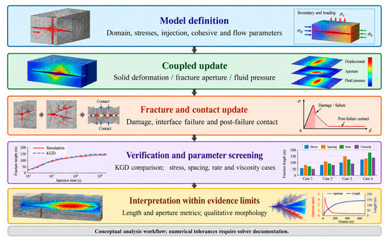
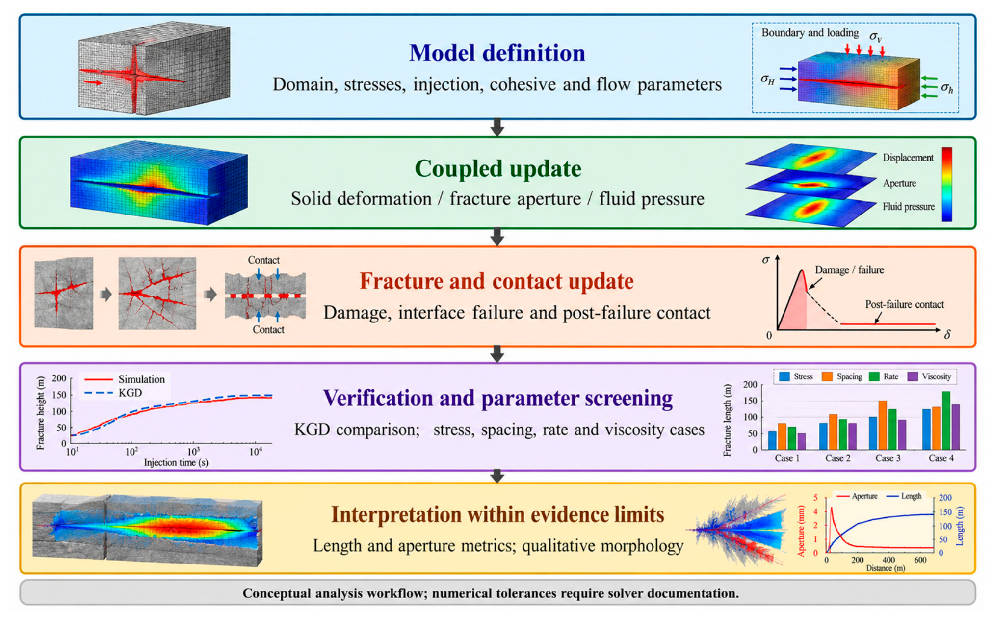
The analysis proceeds through model definition, coupled mechanics and flow updates, fracture/contact evolution, benchmark comparison and case interpretation (Figure 1). The flow and deformation fields are mutually dependent through pressure loads and aperture-dependent conductivity. The workflow describes these dependencies at the formulation level; it does not establish a particular subcycling ratio, convergence tolerance or stopping criterion for the reported calculations.

Figure 1. The conceptual workflow for the coupled formulation, benchmark comparison and parameter screening.

2.5. Quantitative Evaluation

All additional statistics below are recalculated from the printed length and aperture values; no new fracture propagation simulations are introduced. For n comparison points, the mean absolute percentage error and root mean square error are defined as follows:

MAPE_X = (100/n) Σ_j|(X_FDEM,j − X_KGD,j)/X_KGD,j|

(22a)

RMSE_X = √[(1/n) Σ_j (X_FDEM,j − X_KGD,j)²]

(22b)

For three non-negative cluster lengths L_i, the total length L_Σ, middle-fracture share f_m, coefficient of variation CV_L and dimensionless uniformity U_L are

L_Σ = Σ_i L_i;  f_m = L_middle/L_Σ

(23a)

CV_L = √[Σ_i(L_i − L)²/3]/L

(23b)

U_L = (Σ_i L_i)²/(3Σ_i L_i²) = 1/(1 + CV_L²)

(24)

For positive total length, U_L ranges from 1/3, when only one cluster grows, to 1 for equal lengths. It measures geometric uniformity and is insensitive to a common multiplicative change in all lengths. It is not an index of conductivity, connected volume or productivity. CV_L uses the population standard deviation of the three clusters; neither statistic is an uncertainty interval. Quantitative branching density would require a branch-counting rule and resolved branch lengths, so it is not calculated from the available images.

3. Results

This section first evaluates the numerical accuracy of the hydro-mechanical FDEM framework using a classical analytical benchmark and then examines the effects of horizontal principal stress differences, cluster spacing, injection rate and fracturing-fluid viscosity on multi-cluster fracture propagation.

3.1. Model Verification Against the KGD Solution

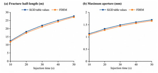
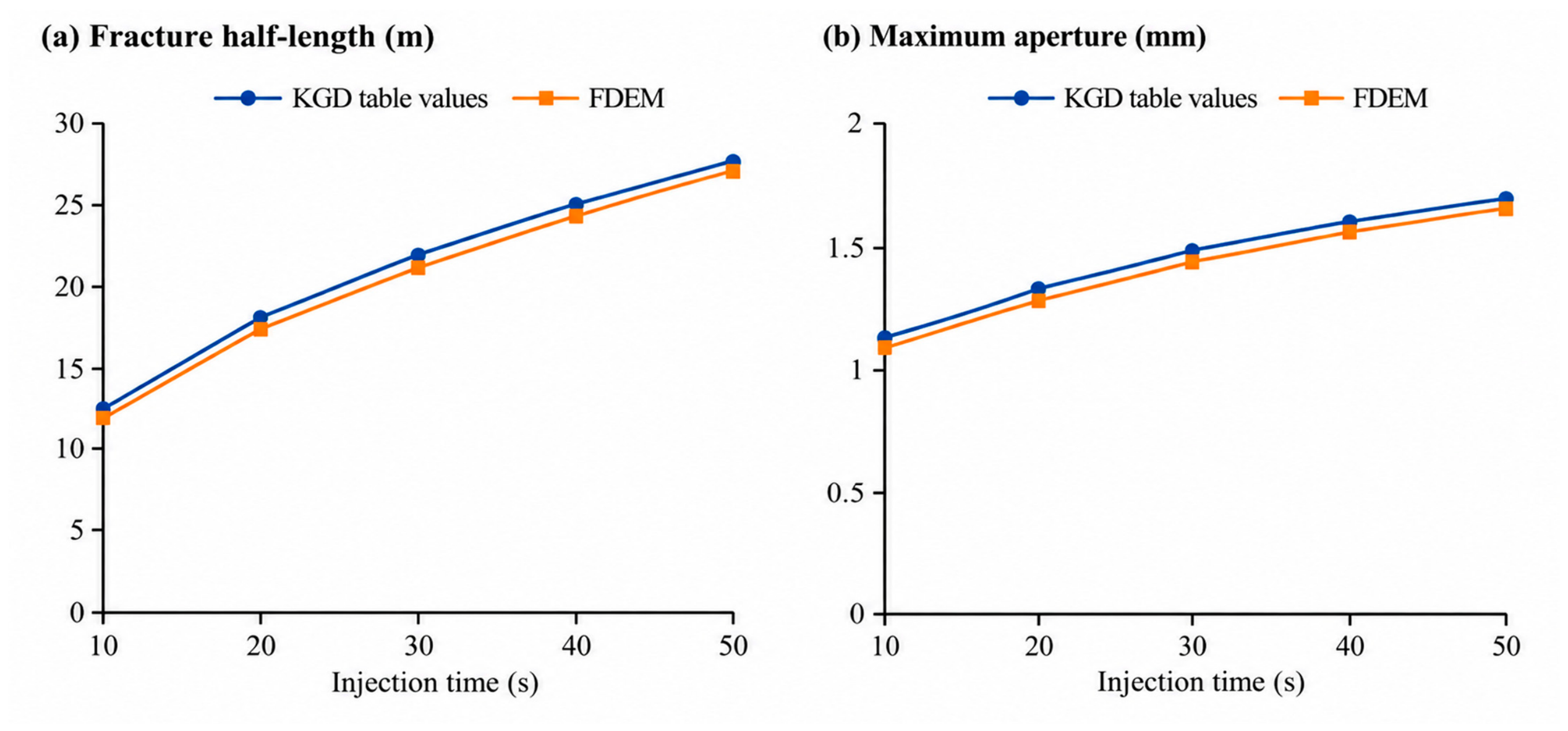
A planar-fracture comparison uses the five pairs of KGD and FDEM half-length and maximum-aperture values in Table 1. The KGD formulation [3] provides the reference context. Figure 2 plots the reported samples at 10, 20, 30, 40 and 50 s; lines connect those samples without interpolating an independently solved analytical model. This comparison tests the two tabulated observables rather than the entire coupled formulation.

Table 1. A comparison of the fracture half-length and maximum aperture predicted by the FDEM and KGD models.

Injection Time/(s)	Half-Length (KGD)/(m)	Half-Length (FDEM)/(m)	Error/(%)	Maximum Fracture Aperture (KGD)/(mm)	Maximum Fracture Aperture (FDEM)/(mm)	Error/(%)
10	12.45	12.11	2.73	1.12	1.15	2.68
20	18.23	17.85	2.08	1.34	1.31	2.24
30	22.11	21.68	1.94	1.48	1.45	2.03
40	25.32	24.91	1.62	1.59	1.57	1.26
50	28.15	27.82	1.17	1.68	1.65	1.79

Figure 2. KGD and FDEM samples from Table 1: (a) fracture half-length; (b) maximum aperture.

Relative errors in half-length range from 1.17% to 2.73%, and those in maximum aperture range from 1.26% to 2.68%. The recalculated MAPE is 1.91% for half-length and 2.00% for aperture. Half-length has an RMSE of 0.380 m and a mean signed difference (FDEM minus KGD) of −0.378 m; every tabulated half-length is slightly underestimated. Aperture has an RMSE of 0.0283 mm and a mean signed difference of −0.0160 mm. These statistics describe the five rounded samples and are not confidence limits. Independent reconstruction of the analytical curve requires the full benchmark regime and inputs, while pressure and spatial-aperture verification require additional field histories. Agreement below 3% is therefore not evidence of mesh-independent branching or verified multi-fracture competition.

3.2. Parametric Analysis of Multi-Cluster Fracture Propagation

The multi-cluster geometry is a 400 m × 200 m domain containing three injection points. The reported case sets vary the horizontal principal stress difference (2, 6, 10 and 14 MPa), cluster spacing (5, 10, 15 and 20 m), volumetric-rate label (3, 6, 9 and 12 m³/min) and viscosity (1, 10, 50 and 100 MPa·s). Table 2 separates directly reported inputs from algebraically derived properties. The case sets are interpreted as comparisons within this two-dimensional setting. Assignment of the separately recorded 0.2 m³/min value, the rate allocation among clusters and the effective height are unresolved; those values cannot be used to infer a unique field pumping schedule.

Table 2. Reported model descriptors and directly derived elastic properties.

Quantity	Value
Domain size	400 m × 200 m
Number of injection points	3
Young’s modulus E	35 GPa
Poisson’s ratio ν	0.25
Shear modulus G	14.0 GPa
Plane-strain modulus E′	37.33 GPa
Bulk modulus K	23.33 GPa
Horizontal stress magnitudes	10 and 17 MPa
Tensile strength σ_t	6.32 MPa
Cluster-spacing cases	5, 10, 15 and 20 m
Stress-difference cases	2, 6, 10 and 14 MPa
Injection-rate cases	3, 6, 9 and 12 m3/min
Viscosity cases	1, 10, 50 and 100 MPa·s
Additional rate entry	0.2 m3/min
Void ratio and porosity entries	e = 0.1; φ = 0.5
Additional leak-off entry	10−6 m3/(Pa·s)

3.2.1. Effect of Horizontal Principal Stress Difference

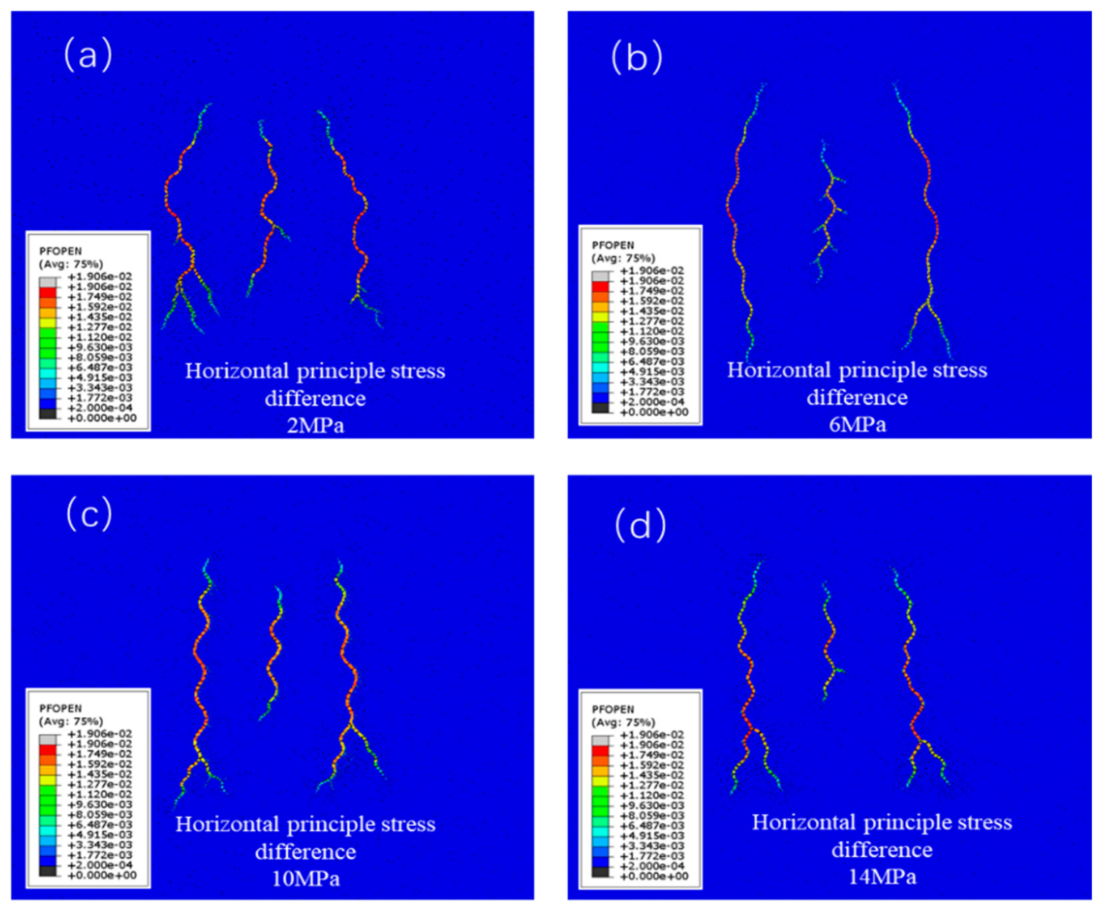
The horizontal principal stress difference was varied from 2 to 14 MPa (Figure 3). Images are interpreted qualitatively as changes in deflection and branching. The reported total fracture length decreases from 215.4 m at 2 MPa to 142.1 m at 14 MPa, a reduction of 34.0%; the 6 MPa case is reported as 187.4 m. A complete four-case numerical series is unavailable. The endpoint trend is consistent with stronger directional constraint at higher stress anisotropy, but fracture appearance alone cannot establish tensile/shear failure fractions or a quantitative stimulated volume.

Figure 3. Fracture patterns for horizontal principal stress differences of (a) 2, (b) 6, (c) 10 and (d) 14 MPa.

3.2.2. Effect of Cluster Spacing

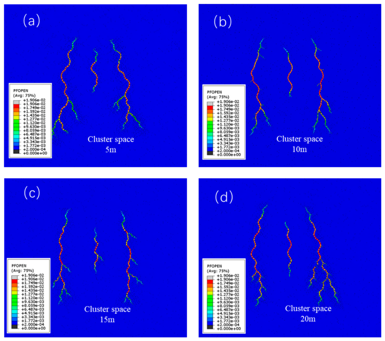
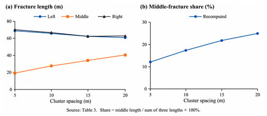
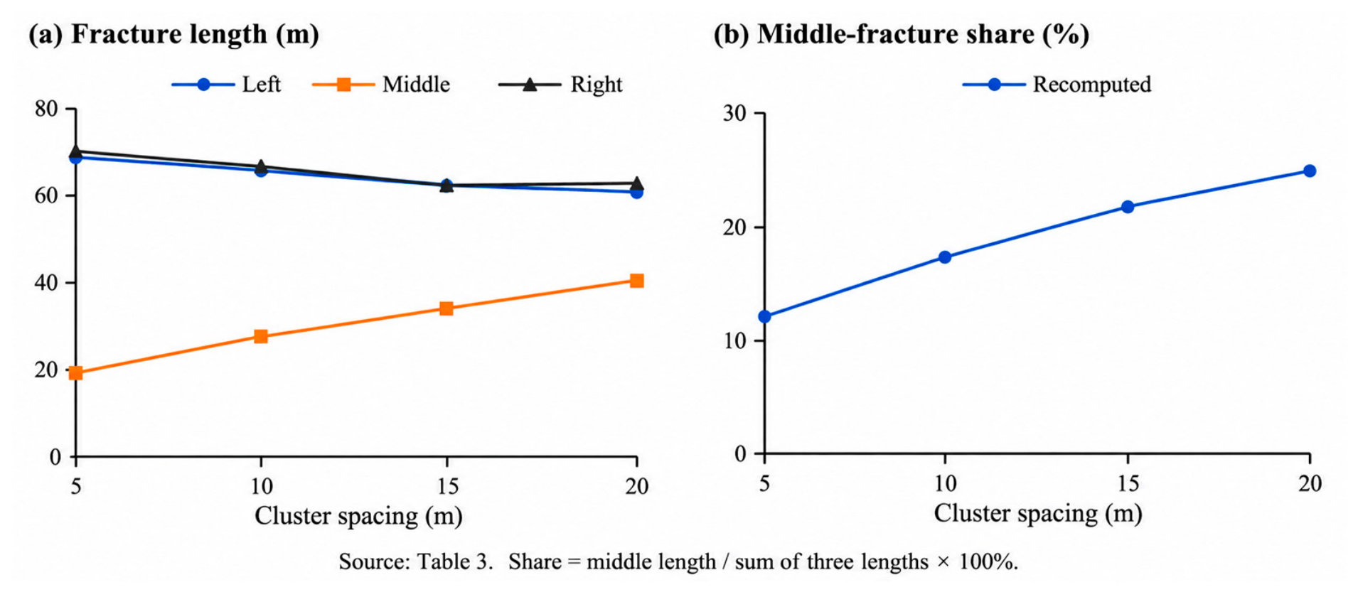
Increasing cluster spacing from 5 to 20 m increases middle-fracture length from 18.5 to 39.8 m, or 115.1% (Table 3 and Figure 4 and Figure 5). Recalculated middle-fracture shares are 11.87%, 17.10%, 21.33% and 24.43%, and total lengths are 155.8, 158.5, 157.5 and 162.9 m, respectively. Thus, total length does not increase monotonically across all four spacings and rises by only 4.6% between the endpoints. Over the same interval, the combined outer-fracture length decreases from 137.3 to 123.1 m, while the middle fracture gains 21.3 m. This identifies redistribution toward the central cluster as the main spacing response. Reduced stress-shadow suppression is a plausible explanation, but direct stress fields are needed to establish its magnitude.

Table 3. Quantitative analysis of fracture propagation lengths under different cluster spacings.

Cluster Spacing (m)	Left-Fracture Length/(m)	Middle-Fracture Length/(m)	Right-Fracture Length/(m)	Middle-Fracture Share (%)
5	68.2	18.5	69.1	11.87
10	65.4	27.1	66.0	17.10
15	62.1	33.6	61.8	21.33
20	60.7	39.8	62.4	24.43

Figure 4. Fracture patterns for cluster spacings of (a) 5, (b) 10, (c) 15 and (d) 20 m.

Figure 5. Recalculated spacing response from Table 3: (a) individual lengths; (b) middle-fracture share.

3.2.3. Effect of Injection Rate

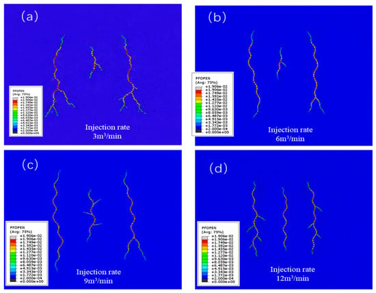
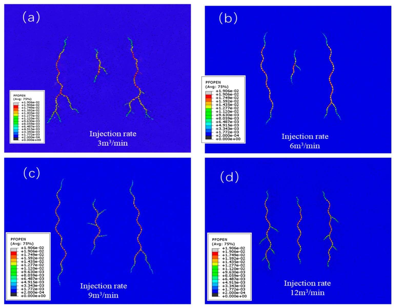
Injection-rate labels of 3, 6, 9 and 12 m³/min define the four cases in Figure 6. The reported maximum aperture increases from 1.4 mm at 6 m³/min to 3.2 mm at 12 m³/min, a factor of 2.29 and an absolute increase of 1.8 mm. The images suggest additional secondary branches at higher rates. Such behavior is consistent with a larger pressure-driven opening force, but no pressure rise is quantified from the aperture endpoints alone. In the absence of documented comparison time and cumulative injected volume, the rate and total-volume effects cannot be separated. This result is therefore an endpoint comparison, not a calibrated rate–aperture scaling law.

Figure 6. Fracture patterns for injection-rate labels of (a) 3, (b) 6, (c) 9 and (d) 12 m³/min.

3.2.4. Effect of Fracturing-Fluid Viscosity

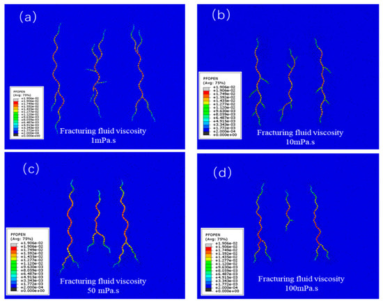
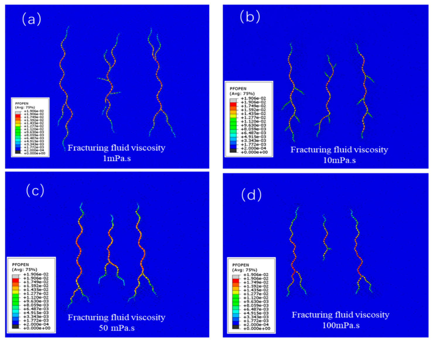
Viscosities of 1, 10, 50 and 100 MPa·s define the cases in Figure 7. At fixed aperture and pressure gradient, cubic-law conductivity varies as μ_l⁻¹; a change from 1 to 100 MPa·s would reduce that conductivity by a factor of 100. Evolving aperture and pressure prevent interpreting this identity as the actual flow-rate ratio. The 100 MPa·s case has a reported average aperture of 2.6 mm, and the images suggest differences in path complexity. These observations support a qualitative opening–morphology trade-off. They do not establish shear/tensile fractions or a numerical branching-frequency reduction. Moreover, Equation (17) contains no explicit viscosity unless C_l is linked to fluid and matrix properties; enhanced leak-off at lower viscosity cannot be inferred from an unchanged Carter coefficient [7].

Figure 7. Fracture patterns for viscosities of (a) 1, (b) 10, (c) 50 and (d) 100 MPa·s.

3.3. Comparison of Combined Parameter Schedules

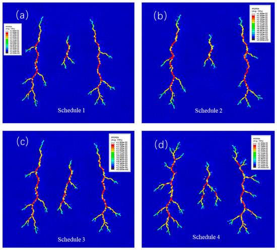
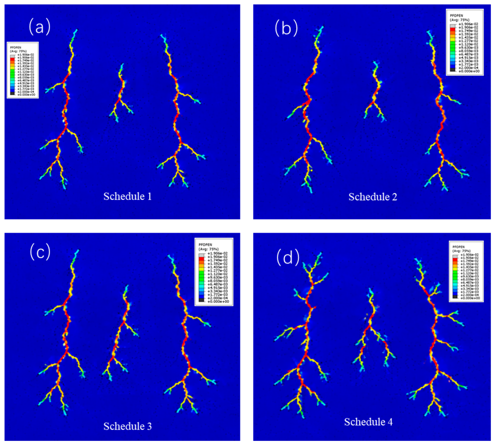
Four combined parameter schedules are listed in Table 4 and illustrated in Figure 8. Schedule 4 uses 10 m spacing, 12 m³/min and 1 MPa·s and appears more branched in the available image. However, Schedules 1–2 vary both rate and viscosity, and Schedules 2–3 vary both spacing and rate. Only Schedules 3–4 hold the listed spacing and rate fixed while changing viscosity, and any causal comparison additionally requires matched time, volume and other inputs. The images therefore motivate candidate combinations for subsequent testing but do not demonstrate a numerical optimum. The listed cases use fixed viscosities and do not test a subsequent slickwater-displacement stage.

Table 4. Combined parameter schedules for qualitative comparison.

Schedule	Cluster Space/m	Injection Rate/m3/min	Viscosity of Fracturing Fluid/MPa·s
1	15	6	50
2	15	9	10
3	10	12	10
4	10	12	1

Figure 8. Fracture patterns for Schedules 1–4 (a–d) in Table 4.

4. Discussion

4.1. Coupled Mechanisms Governing Multi-Cluster Fracture Growth

The spacing results distinguish growth redistribution from total extension. CV_L decreases from 0.455 at 5 m spacing to 0.189 at 20 m, and the equivalent U_L increases from 0.828 to 0.965 (Table 5). The middle-to-mean-outer length ratio rises from 0.269 to 0.647 but remains below unity, indicating persistent central suppression even in the widest tested case. A more even distribution does not imply that the middle fracture has reached parity or that total connected fracture area has been maximized. The derived metrics are deterministic summaries of the three lengths rather than independent measurements of stress shadow or fluid allocation.

Table 5. Recalculated growth-distribution indicators for the four spacing cases.

Spacing (m)	Total Length (m)	Middle Share (%)	CV_L	U_L	Middle/Mean Outer
5	155.8	11.87	0.455	0.828	0.269
10	158.5	17.10	0.344	0.894	0.412
15	157.5	21.33	0.255	0.939	0.542
20	162.9	24.43	0.189	0.965	0.647

Mechanistic tests require additional field variables. A possible stress–shadow ratio is χ = Δσ_shadow/p_net, with both quantities evaluated at a specified location and time and with positive compressive shadow stress and positive net pressure. The flow fraction η_i = Q_i/ΣQ_i measures injection partitioning. Neither ratio can be evaluated from length images alone. Trends are consistent with stress interaction and fluid redistribution, but no critical χ threshold or measured flow competition is claimed. Quantifying branching requires a reproducible branch definition, a physical minimum length and a common comparison time or injected volume.

4.2. Implications for Hydraulic-Fracturing Design

A design objective must specify whether the aim is balanced cluster growth, total connected length, aperture, proppant placement or production. For length uniformity alone, 20 m has the highest U_L among the four reported spacing cases. This ranking is not optimal for treatment efficiency, because greater spacing can reduce cluster density and the available data do not quantify connected area or productivity per unit well length. Likewise, U_L cannot rank the four combined schedules without their individual cluster lengths. A defensible multi-objective comparison would use common time or injected-volume conditions and report geometry together with pressure work and proppant transport. The present results identify candidate trends for that comparison rather than a final treatment design.

4.3. Model Limitations and Future Work

The two-dimensional geometry suppresses vertical growth and cannot represent layer-controlled height containment or out-of-plane stress redistribution. In three dimensions, injected volume can be accommodated by height growth and in-plane extension and opening. The fixed-height approximation can overstate in-plane growth if appreciable height growth would occur, whereas containment can alter pressure and shadow extent in a different direction. The net bias in cluster competition is case-dependent and cannot be quantified here. A two-dimensional fracture area must not be interpreted as a stimulated reservoir volume.

A homogeneous, isotropic, linear-elastic matrix omits bedding, spatially variable strength, natural fractures and distributed inelastic deformation. These features can redirect fractures and change initiation thresholds, pressure dissipation and branching. Simulated branches on predefined cohesive interfaces may partly reflect the discretization. Without refinement and mesh-orientation studies, morphology and branch counts cannot be regarded as mesh-independent.

The incompressible Newtonian fluid assumption omits compressibility, non-Newtonian rheology and multiphase flow. These omissions can change storage, transient pressure, leak-off and flow partitioning; the direction and magnitude depend on fluid properties and operating conditions. The Carter closure cannot be treated as a universally pressure-dependent matrix-flow model. Its role and parameters must be reconciled with the matrix Darcy equation.

The five-point KGD comparison does not establish spatial or temporal convergence. Mesh, time-step and cohesive-parameter studies, cumulative mass-balance output and pressure histories are absent from the reported result set. In addition, the interface exchange closure, porosity, rate conversion and parts of the solver input specification remain unresolved. These gaps prevent independent reproduction and cannot be filled by adopting parameters from a different study. Literature-informed values would define new simulations requiring their own verification. Accordingly, the results are restricted to the reported geometry and aperture comparisons. Mesh-orientation and process-zone resolution studies, laboratory or field diagnostics and three-dimensional cases are necessary before predictive treatment-design use.

5. Conclusions

A two-dimensional FDEM framework and its reported multi-cluster cases were examined using consistent length and aperture metrics. The main findings, within the limitations of the available numerical record, are as follows:

(1)

The five tabulated KGD/FDEM comparisons have maximum relative errors of 2.73% in half-length and 2.68% in maximum aperture. Corresponding MAPE values are 1.91% and 2.00%. This is in agreement for selected observables, not proof of convergence or validated branching.

(2)

Increasing spacing from 5 to 20 m increases the middle-fracture length by 115.1% and its length share from 11.87% to 24.43%, while total length increases by only 4.6%. U_L increases from 0.828 to 0.965. The dominant quantitative response is more uniform growth rather than a comparable expansion of total length.

(3)

Maximum aperture increases from 1.4 to 3.2 mm between the reported 6 and 12 m³/min cases. This endpoint trend is compatible with stronger opening but does not isolate rate from injected-volume effects or establish a field-scale pumping recommendation.

(4)

The reported total length decreases from 215.4 to 142.1 m between the low- and high-stress-difference endpoints, and the viscosity cases suggest morphology changes. Quantitative failure-mode, branching and leak-off attributions require additional field outputs.

(5)

The combined schedules provide qualitative parameter screening. No common score or temporal fluid-switching experiment supports a treatment optimum. Conservative implementation, complete input documentation and discretization verification remain essential before the framework can be used predictively.

References

- Zeng, J.; Wang, X.; Guo, J.; Zeng, F.; Zhang, Q. Composite linear flow model for multi-fractured horizonal wells in tight sand reservoirs with the threshold pressure gradient. J. Pet. Sci. Eng. 2018, 165, 890–912. [Google Scholar] [CrossRef] [Scilit]
- Wang, Z.; Lou, Y.; Pan, J. China’s Oil & gas resources exploration and development and its prospect. Int. Pet. Econ. 2017, 25, 1–6. [Google Scholar]
- Wang, K.; Zhang, H.L.; Zhang, R.H.; Wang, J.P.; Dai, J.S.; Yang, X.J. Characteristics and influencing factors of ultra-deep tight sandstone reservoir structural fracture: A case study of Keshen-2 gas field, Tarim Basin. Acta Petrol. Sin. 2016, 37, 715–727, 742. [Google Scholar]
- Yang, T.; Zhang, G.S.; Liang, K.; Zheng, M.; Guo, B.C. The exploration of global tight sandstone gas and forecast of the development tendency in China. Strateg. Study CAE 2012, 14, 64–68, 76. [Google Scholar]
- Zeng, L.B.; Ke, S.Z.; Liu, Y. Research Methods of Low Permeability Oil and Gas Reservoir Fractures; Petroleum Industry Press: Beijing, China, 2010; pp. 1–187. [Google Scholar]
- Olson, J.E.; Laubach, S.E.; Eichhubl, P. Estimating natural fracture producibility in tight gas sandstones, coupling diagenesis with geomechanical modeling. Lead. Edge 2010, 29, 1494–1499. [Google Scholar] [CrossRef] [Scilit]
- Zeng, L.; Lyu, W.; Li, J.; Zhu, L.; Weng, J.; Yue, F.; Zu, K. Natural fractures and their influence on shale gas enrichment Sichuan Basin, China. J. Pet. Sci. Eng. 2016, 30, 1–9. [Google Scholar] [CrossRef] [Scilit]
- Lyu, W.; Zeng, L.; Zhang, B.; Miao, F.; Lyu, P.; Dong, S. Influence of natural fractures on gas accumulation in the Upper Triassic tight gas sandstones in the northwestern Sichuan Basin, China. Mar. Pet. Geol. 2017, 83, 60–72. [Google Scholar] [CrossRef] [Scilit]
- Fisher, M.K.; Wright, C.A.; Davidson, B.M.; Goodwin, A.K.; Fielder, E.O.; Buckler, W.S.; Steinsberger, N.P. Integrating fracture mapping technologies to optimize stimulations in the Barnett shale. In Proceedings of the SPE Annual Technical Conference and Exhibition, San Antonio, TX, USA, 29 September–2 October 2002. Paper Number: SPE-77441. [Google Scholar]
- Maxwell, S.C.; Urbancic, T.I.; Steinsberger, N.; Zinno, R. Microseismic imaging of hydraulic fracture complexity in the barnett shale. In Proceedings of the SPE Annual Technical Conference and Exhibition, San Antonio, TX, USA, 29 September–2 October 2002. Paper Number: SPE-77440. [Google Scholar]
- Perkins, T.K.; Kern, L.R. Width of hydraulic fractures. J. Pet. Technol. 1961, 13, 937–949. [Google Scholar] [CrossRef] [Scilit]
- AbuAisha, M.; Eaton, D.; Priest, J.; Wong, R. Hydro-mechanically coupled FDEM framework to investigate near-wellbore hydraulic fracturing in homogeneous and fractured rock formations. J. Pet. Sci. Eng. 2017, 154, 100–113. [Google Scholar] [CrossRef] [Scilit]
- Yan, C.; Jiao, Y.-Y. A 2D fully coupled hydro-mechanical finite-discrete element model with real pore seepage for simulating the deformation and fracture of porous medium driven by fluid. Comput. Struct. 2018, 196, 311–326. [Google Scholar] [CrossRef] [Scilit]
- Yan, C.; Zheng, H. Three-Dimensional Hydromechanical Model of Hydraulic Fracturing with Arbitrarily Discrete Fracture Networks using Finite-Discrete Element Method. Int. J. Geomech. 2017, 17, 04016133. [Google Scholar] [CrossRef] [Scilit]
- Osiptsov, A.A. Fluid Mechanics of Hydraulic Fracturing: A Review. J. Pet. Sci. Eng. 2017, 156, 513–535. [Google Scholar] [CrossRef] [Scilit]
- Zhang, G.; Sun, S.; Chao, K.; Niu, R.; Liu, B.; Li, Y.; Wang, F. Investigation of the nucleation, propagation and coalescence of hydraulic fractures in glutenite reservoirs using a coupled fluid flow-DEM approach. Powder Technol. 2019, 354, 301–313. [Google Scholar] [CrossRef] [Scilit]
- Chen, M.; Sun, Y.; Fu, P.; Carrigan, C.R.; Lu, Z.; Tong, C.H.; Buscheck, T.A. Surrogate-based optimization of hydraulic fracture in pre-existing fracture networks. Comput. Geosci. 2013, 58, 69–79. [Google Scholar] [CrossRef] [Scilit]
- Wang, H.Y. Hydraulic fracture propagation in naturally fractures reservoirs: Complex fracture or fracture networks. J. Nat. Gas. Sci. Eng. 2019, 68, 102911. [Google Scholar] [CrossRef] [Scilit]
- Wei, Y.; Wang, J.; Yu, W.; Qi, Y.; Miao, J.; Yuan, H.; Liu, C. A smart productivity evaluation method for shale gas wells based on 3D fractal fracture network model. Pet. Explor. Dev. 2021, 48, 787–796. [Google Scholar] [CrossRef] [Scilit]
- Wan, X.; Rasouli, V.; Damjanac, B.; Yu, W.; Xie, H.; Li, N.; Rabiei, M.; Miao, J.; Liu, M. Coupling of fracture model with reservoir to simulate shale gas production with complex fractures and nanopores. J. Pet. Sci. Eng. 2020, 193, 107422. [Google Scholar] [CrossRef] [Scilit]
- Sobhaniaraghn, B.; Mansur, W.J.; Peter, F.C. Three-dimensional investigation of multiple stage hydraulic fracturing in unconventional reservoirs. J. Pet. Sci. Eng. 2016, 146, 1063–1078. [Google Scholar] [CrossRef] [Scilit]
- Khoei, A.R.; Vahab, M.; Ehsani, H.; Rafieerad, M. XFEM modeling of large plasticity deformation; a convergence study on various blending strategies for weak discontinuities. Eur. J. Comput. Mech. 2015, 24, 79–106. [Google Scholar] [CrossRef] [Scilit]
- Hanks, C.L.; Lorenz, J.; Teufel, L.; Krumhardt, A.P. Lithologic and structural controls on natural fracture distribution and behavior within the Lisburne Group, northeastern Brooks Range and North Slope subsurface, Alaska. AAPG Bull. 1997, 81, 1700–1720. [Google Scholar] [CrossRef] [Scilit]
Disclaimer/Publisher’s Note: The statements, opinions and data contained in all publications are solely those of the individual author(s) and contributor(s) and not of MDPI and/or the editor(s). MDPI and/or the editor(s) disclaim responsibility for any injury to people or property resulting from any ideas, methods, instructions or products referred to in the content. |
© 2026 by the authors. Licensee MDPI, Basel, Switzerland. This article is an open access article distributed under the terms and conditions of the Creative Commons Attribution (CC BY) license.