A Machine Learning Framework for Predicting Fracture Dip Angle in Shale Gas Reservoirs from Pulsed Neutron Logging Responses

Abstract

Accurate characterization of fracture angles is crucial for evaluating natural gas storage and transport capacity in shale gas reservoirs. Although numerical simulations based on neutron transport theory can model well log responses at different fracture angles, the process is computationally intensive and is not suitable for field applications. This study proposes a data-driven machine learning (ML) framework to rapidly and accurately predict fracture dip angles directly from pulsed neutron logging measurements. We generated a comprehensive dataset using a high-fidelity deterministic neutron transport solver based on the discrete ordinate method. This solver provides a direct solution to the Boltzmann transport equation, simulating thermal and epithermal neutron fluxes, energy spectra, and time-dependent distributions across fracture angles ranging from 0° to 90°. Key features, including effective fracture volume (EFV), neutron count ratios, and spectral energy centroids, were extracted. We developed and compared three regression models: Random Forest (RF), Support Vector Regression (SVR), and a Deep Neural Network (DNN). The DNN model outperformed traditional approaches, achieving a coefficient of determination (R²) of 0.98 on the test dataset. Feature importance analysis using SHAP confirmed that the ratio of epithermal to thermal neutron counts and the high-energy tail (>7 MeV) of the neutron spectrum are the most discriminative features for distinguishing high-angle (>60°) from low-angle (<30°) fractures. The proposed ML framework provides a robust surrogate model for the computationally expensive neutron transport simulation, enabling real-time interpretation of fracture orientation from well logs. This approach offers a novel methodology for porosity correction and reservoir quality assessment in unconventional shale gas formations.

1. Introduction

Shale gas reservoirs have emerged as a cornerstone of global unconventional hydrocarbon production, owing to their vast resource potential and the technological advancements in drilling technology and hydraulic fracturing [1,2,3]. Unlike conventional reservoirs, the economic viability of shale gas extraction hinges critically on the presence and connectivity of natural fracture networks [4]. These fractures serve a dual purpose: they act as primary conduits for gas migration from the nano-Darcy matrix permeability to the wellbore, and they constitute significant storage volume for free gas [5]. Consequently, the accurate characterization of fracture properties, particularly their orientation or dip angle, is paramount for estimating original gas in place, optimizing well placement, and predicting long-term production decline curves [6].

Among the suite of downhole evaluation techniques, nuclear logging, specifically pulsed neutron logging (PNL), provides unique and invaluable insights into formation porosity, lithology, and fluid saturation independent of borehole rugosity and salinity effects [7,8]. In the context of fractured media, the presence of gas-filled fractures introduces significant perturbations in the neutron transport process. Hydrogen, primarily associated with formation water, hydrocarbons, and clay-bound water, is the most effective moderator of fast neutrons. However, natural gas within fractures exhibits a substantially lower hydrogen index than the surrounding rock matrix or water-filled pores. Therefore, variations in fracture volume intersecting the tool’s radius of investigation manifest as localized increases in neutron count rates.

Despite the clear physical coupling between fracture geometry and neutron log response, the operational interpretation of such logs in highly deviated or fractured intervals remains a non-trivial problem. Traditional deterministic inversion schemes rely on iterative forward simulations [9,10,11]. These forward models are extremely computationally intensive. Furthermore, the relationship between observed logging parameters (such as count ratios and time decay constants) and actual fracture dip angles is highly nonlinear and multivariate, often exceeding the capabilities of simple empirical chart calibration.

Advances in data science in recent years have established machine learning (ML) as a transformative tool in the field of underground characterization [12,13,14,15]. Supervised learning algorithms excel at extracting complex, high-dimensional correlations from labeled datasets without requiring an explicit analytical expression for the underlying physical processes. At the same time, machine learning models trained using offline simulated databases can serve as efficient surrogate models or simulators, thereby offering a highly promising approach to overcoming the computational bottlenecks associated with traditional well logging inversion.

However, no robust machine learning framework has yet been established to fully capitalize on the subtle, physically driven features identified in high-fidelity deterministic simulations-such as the surge in high-energy neutron flux in environments with high-angle fractures. To address this gap, this study proposes a novel data-driven framework for directly predicting fracture inclination angle from PNL measurement data. This work makes three specific contributions: 1. High-Fidelity Deterministic Database Construction: We develop an extensive synthetic logging database by solving the multi-group neutron transport equation using the discrete ordinates method across a comprehensive parameter space of fracture angles. This approach yields a noise-free, physics-constrained training corpus. 2. Feature Engineering based on Neutron Transport Physics: We derive and evaluate a suite of physics-guided features, including spectral energy integrals (specifically the 7–13 MeV tail) and time spectrum decay characteristics, which serve as robust proxies for the Effective Fracture Volume. 3. Development and Interpretation of a Deep Learning Surrogate Model: We construct and benchmark a Deep Neural Network (DNN) against conventional regression models. Furthermore, we employ SHAP to deconvolve the “black box” nature of the ML model, thereby validating that the model’s internal logic aligns with the established physical principle of EFV.

2. Numerical Simulation Methodology and Feature Extraction Framework

This section delineates the computational workflow employed to generate the synthetic pulsed neutron logging (PNL) dataset and the subsequent feature extraction protocol.

2.1. Deterministic Neutron Transport Simulation Framework

2.1.1. Governing Equation and Discretization Schemes

The migration of neutrons through the borehole-formation system is governed by the time-dependent, multi-group Boltzmann transport equation. For a given energy group $g$ and angular direction ${\mathsf{\Omega }}_m$, the steady-state form can be expressed as:

$${\mathsf{\Omega }}_m·\nabla {\psi }_g\left(\mathit{r},{\mathsf{\Omega }}_m\right)+{\sum }_{t,g}\left(\mathit{r}\right){\psi }_g\left(\mathit{r},{\mathsf{\Omega }}_m\right)=Q_g\left(\mathit{r},{\mathsf{\Omega }}_m\right)$$

(1)

where ${\psi }_g\left(\mathit{r},{\mathsf{\Omega }}_m\right)$ denotes the angular neutron flux for group $g$ at spatial position $\mathit{r}$ along discrete direction ${\mathsf{\Omega }}_m$. ${\sum }_{t,g}\left(\mathit{r}\right)$ is the macroscopic total cross-section. $Q_g\left(\mathit{r},{\mathsf{\Omega }}_m\right)$ represents the total source term, encompassing the external D-T generator source, in scattering contributions from other energy groups, and fission sources.

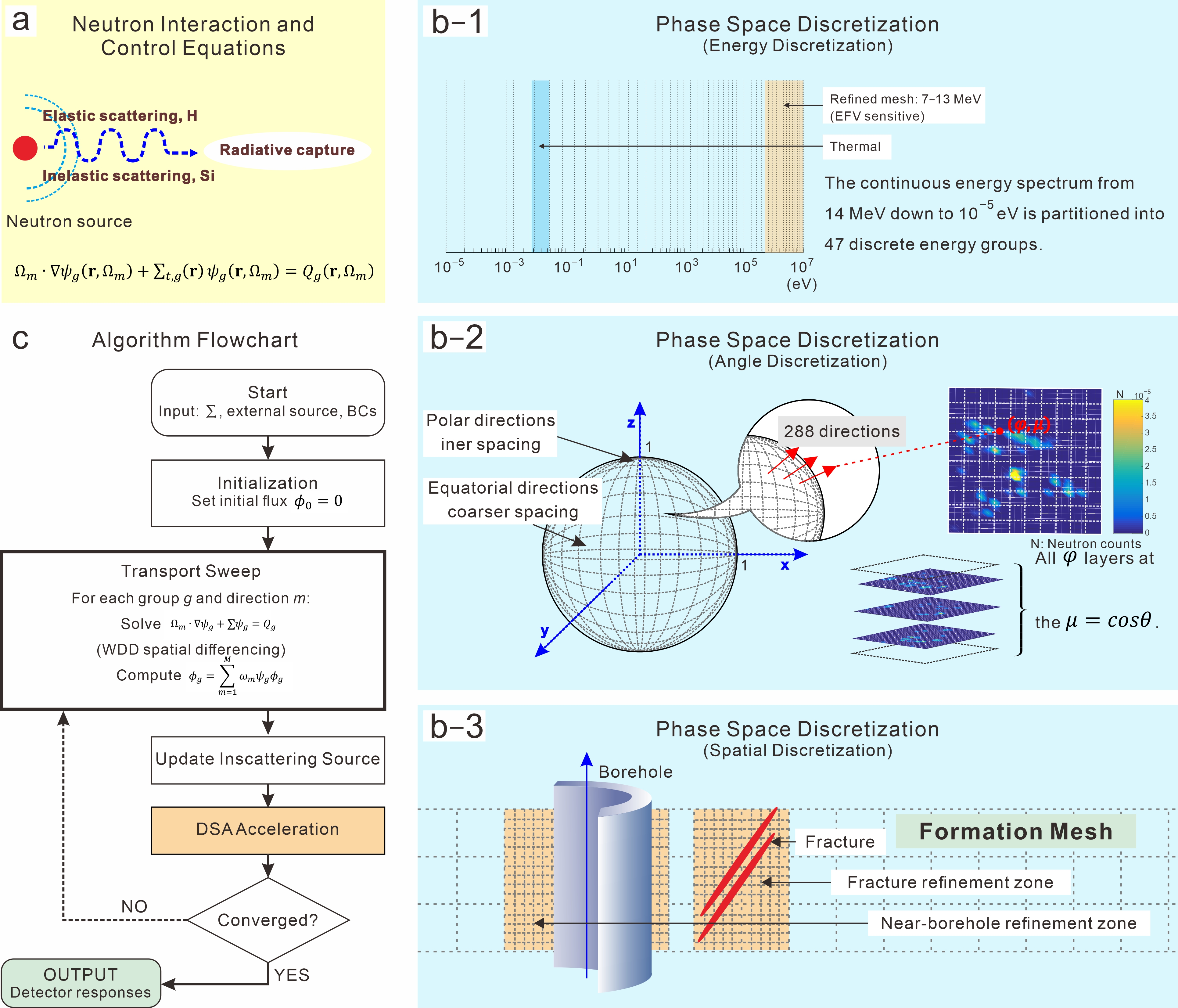
To resolve this equation accurately while avoiding the statistical noise inherent in stochastic particle transport methods, a deterministic multi-group discrete ordinates approximation is employed. The discretization strategy is configured as follows (Figure 1): 1. Energy Discretization: The continuous energy spectrum from 14 MeV down to 10⁻⁵ eV is partitioned into 47 discrete energy groups. 2. Angular Discretization: The unit sphere of neutron flight directions is discretized, resulting in a total of 288 discrete ordinates. 3. Spatial Discretization and Solver: The spatial domain is decomposed using a cylindrical structured mesh with radial refinement near the borehole wall and fracture interfaces. The transport equation is solved via the Source Iteration method, accelerated by Diffusion Synthetic Acceleration to expedite convergence in regions characterized by high scattering ratios. The solution yields the scalar neutron flux ${\varphi }_g(\mathit{r})$ for each energy group, defined as:

$${\varphi }_g\left(\mathit{r}\right)={\sum }_{m=1}^M{\omega }_m{\psi }_g({\varphi }_g(\mathit{r},{\mathsf{\Omega }}_m)$$

(2)

where ${\omega }_m$ are the quadrature weights associated with direction ${\mathsf{\Omega }}_m$.

Figure 1. Schematic of the deterministic neutron transport framework. (a) Neutron interactions and the steady-state multigroup Boltzmann transport equation; (b) Phase-space discretization: b–1. 47-group energy structure, b–2. Angle-discrete integration set, b–3. Cylindrical structured mesh with fracture detail. (c) Iterative solution algorithm with source iteration and diffusion synthetic acceleration (DSA).

The multi-group macroscopic cross-sections were generated from the ENDF/B- -VIII.0 evaluated nuclear data library. The energy range was partitioned into 47 neutron groups with refinement in the 7–13 MeV interval. The group-averaged cross-sections for each constituent nuclide were produced using the NJOY processing code with a flux-weighted condensation spectrum consistent with the formation environment.

Calculations used full 3D cylindrical coordinates ($r, \phi , z$) with non-axisymmetric inclined fractures. The azimuthal domain [0, 2$\pi$) was discretized into 64 uniform cells; a convergence test showed <$0.3\%$ change in detector count rate when doubled, so 64 cells were used.

The angular discretization employs a level-symmetric S₁₆ quadrature set, consisting of 288 discrete ordinates. The quadrature weights and direction cosines are generated using the standard level-symmetric construction. A quadrature-refinement study comparing S₈, S₁₂, and S₁₆ showed that the S₁₆ set produces detector count rates within 0.2% of the S₂₀ reference, confirming angular convergence. The S₁₆ quadrature was therefore adopted for all simulations.

2.1.2. Temporal Response Modeling

To derive the time-spectrum features, the steady-state flux solution is extended into the time domain. The time-dependent flux $\varphi (t)$ is expressed as a superposition of exponentially decaying spatial eigenmodes ${\varphi }_n\left(\mathit{r}\right)$ with corresponding decay constants ${\lambda }_n$:

$$\varphi \left({\mathit{r}}_d,t\right)={\sum }_{n=1}^{\infty }{A}_n{\varphi }_n({\mathit{r}}_d)e^{-{\lambda }_{n}t}$$

(3)

2.1.3. Point Source in an Infinite Homogeneous Medium

To validate the spatial discretization and the convergence of the deterministic transport solver toward the diffusion limit, we considered a classical benchmark problem: a point source in an infinite homogeneous medium. A 14.1 MeV neutron source was placed at the origin of an infinite water medium, and the thermal neutron flux was computed along the radial direction.

The reference solution is given by the diffusion-theory analytical expression for a point source in an infinite medium:

$${\varphi }_{\mathrm{r}\mathrm{e}\mathrm{f}}\left(\mathit{r}\right)={\displaystyle \frac{S}{4\pi D\mathit{r}}}\mathrm{e}\mathrm{x}\mathrm{p}(-{\displaystyle \frac{\mathit{r}}{L}})$$

(4)

where $S$ is the source strength, D is the diffusion coefficient, and L is the diffusion length. For thermal neutrons in water, D = 0.160 cm and L = 2.85 cm. The calculated thermal neutron flux at five radial distances (5, 10, 15, 20, and 25 cm) is compared with the reference solution in Table 1. The relative error remains below 2.0% over the entire range, confirming that the deterministic transport solver accurately reproduces the spatial decay of the neutron field in a homogeneous medium.

Table 1. Point-source benchmark in an infinite homogeneous water medium: comparison of calculated and reference thermal neutron flux.

Radial Distance r (cm)	Calculated Flux (10−6)	Reference Flux (10−6)	Relative Error (%)
5	1.842	1.856	0.75
10	0.732	0.741	1.21
15	0.301	0.306	1.63
20	0.124	0.126	1.59
25	0.051	0.052	1.92

2.2. Geological Model and Computational Domain Specifications

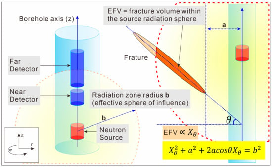
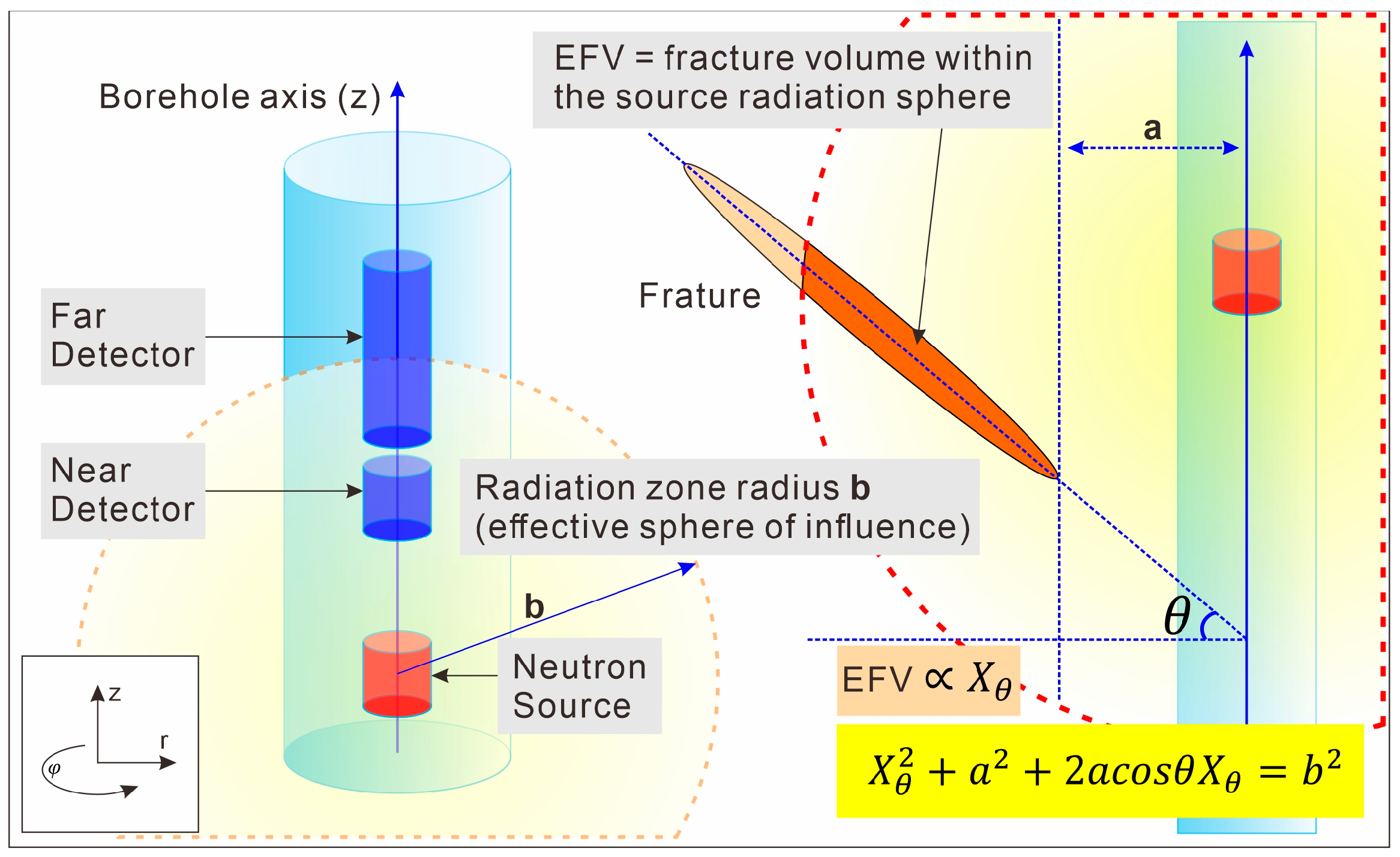
A three-dimensional view of the computational domain is shown: a vertical borehole (diameter 16 cm) containing a D-T pulsed neutron source and two detectors is embedded in a gas-saturated fractured shale formation. The neutron source is a deuterium-tritium pulsed generator emitting 14.1 MeV neutrons with a pulse width of 10 $\mathsf{\mu }\mathrm{s}$ and a repetition period of 1000 $\mathsf{\mu }\mathrm{s}$. The source is modeled as an isotropic point emitter located at the center of the borehole axis. Two neutron detectors are modeled at source distances of 45 cm and 60 cm along the tool axis. The detector response functions are computed as the scalar flux integrated over the respective sensitive volumes, weighted by the energy-dependent detection efficiency curves for ³He proportional counters (thermal) and epithermal detectors with cadmium shielding. Time-gated counting is simulated by integrating the flux over sequential time bins of 10 $\mathsf{\mu }\mathrm{s}$ width. Fracture planes intersect the borehole at a uniform dip angle $\theta$. The translucent blue hemisphere represents the source radiation zone of radius $b$, within which fracture-hosted gas can interact with neutrons. The EFV is quantified by the fracture length $X_{\theta }$ that falls inside the radiation sphere, which is a function of the dip angle $\theta$, the radial offset $a$, and the radiation radius $b$. The geometric relationship $X_{\theta }^2+a^2+2acos\theta X_{\theta }=b^2$ is annotated.

The numerical model replicates the borehole-formation geometry illustrated in Figure 2 of the foundational study [6]. Key dimensional and compositional parameters are summarized in Table 2.

Figure 2. Integrated schematic of the fractured borehole environment and the effective fracture volume (EFV) concept.

Table 2. Computational Domain Parameters.

Parameter Category	Value/Description
Well diameter	16.0 cm
Fluid in well	Freshwater
Instrument diameter	6.0 cm
Main rock type	Siliceous shale/Mudstone
Fracture-filling fluid	Methane
Fracture dip angle	0–90°
Boundary condition-outer radial boundary	Vacuum (zero incoming angular flux)
Boundary condition-top and bottom boundary	Vacuum (zero incoming angular flux)

The fracture geometry is idealized as a set of parallel, planar discontinuities intersecting the borehole at a uniform dip angle $\theta$. While natural fractures exhibit stochastic variability in aperture and spacing, this idealized configuration isolates the first-order effect of orientation on the neutron flux distribution, consistent with the objective of this investigation.

2.3. Dataset Construction Strategy

A parametric sweep over the fracture dip angle $\theta$ constitutes the primary axis of variation in the synthetic database. To enhance the robustness and generalization capacity of the machine learning models, we introduce controlled perturbations to the background matrix composition and borehole environmental parameters.

Primary parameter sweep: Fracture dip angle $\theta \in \left\{0°,5°,10°,\dots ,90°\right\}$, yielding 19 base geometric configurations.

Stochastic perturbations for augmentation: For each base angle, we generate 50 augmented realizations by randomly varying the following parameters within physically plausible bounds: 1. Matrix clay volume fraction: $\pm 8\%$ (relative); 2. Borehole fluid salinity: 0–50 kppm NaCl (uniform distribution); 3. Background formation porosity: $\pm 1.5\%$ (absolute).

This procedure yields a total of 19 × 50 = 950 independent deterministic transport simulations. The dataset is subsequently partitioned into a training set (70%), a validation set (15%), and a hold-out test set (15%). Stratified sampling based on the target angle $\theta$ ensures balanced representation across low-angle (0–30°), intermediate-angle (35–55°), and high-angle (60–90°) regimes.

Distributions and bounds: Clay volume fraction follows a uniform distribution within ±8% relative; borehole salinity follows a uniform distribution from 0 to 50 kppm NaCl; matrix porosity follows a Gaussian distribution with ±1.5% absolute standard deviation. These bounds were chosen to encompass typical ranges reported for shale gas reservoirs while avoiding extreme values that would violate the assumed lithology.

Randomness control: All perturbations were generated using NumPy’s PCG64 generator with a fixed seed (42) to ensure exact reproducibility. The same seed was used across all 19 base angles.

2.4. Feature Extraction and Engineering Protocol

From each deterministic simulation, we extract a suite of physically interpretable features derived from the scalar flux distributions at the two detector locations. The feature vector ${\mathbf{x}}_i$ associated with the i-th simulation instance is composed of the following 22 attributes.

2.4.1. Count Rate and Ratio Features

These features directly correspond to standard PNL log deliverables (Table 3):

Table 3. Definitions and formulas of neutron detection parameters.

Parameter Category	Value/Description
$N_{\mathrm{e}\mathrm{p}\mathrm{i},\mathrm{n}\mathrm{e}\mathrm{a}\mathrm{r}}$, $N_{\mathrm{e}\mathrm{p}\mathrm{i},\mathrm{f}\mathrm{a}\mathrm{r}}$	Epithermal neutron count rate of the near or far detector
$N_{\mathrm{t}\mathrm{h},\mathrm{n}\mathrm{e}\mathrm{a}\mathrm{r}}$, $N_{\mathrm{t}\mathrm{h},\mathrm{f}\mathrm{a}\mathrm{r}}$	Thermal neutron count rate of the near or far detector
$R_{\mathrm{e}/\mathrm{t}\mathrm{h},\mathrm{n}\mathrm{e}\mathrm{a}\mathrm{r}}$	Ratio of epithermal to thermal neutron counts for the near detector
$R_{\mathrm{e}/\mathrm{t}\mathrm{h},\mathrm{f}\mathrm{a}\mathrm{r}}$	Ratio of epithermal to thermal neutron counts for the far detector
$∆R=\mathrm{l}\mathrm{n}(N_{\mathrm{n}\mathrm{e}\mathrm{a}\mathrm{r}/\mathrm{f}\mathrm{a}\mathrm{r}})$	Near-to-far count ratio for neutrons
$I_{\mathrm{H}\mathrm{E}}$	Ratio of the high-energy neutron flux integral to the total neutron flux integral

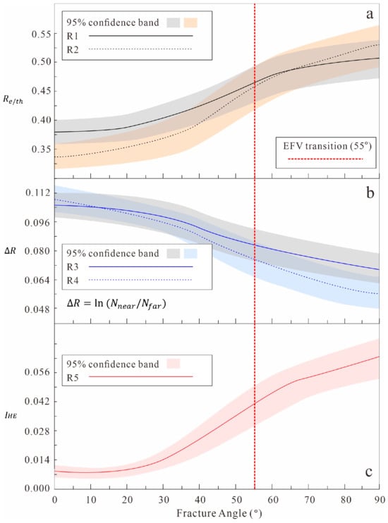
All ratios are derived from the deterministic transport simulation database. The vertical dashed line at 55° highlights the transition zone of the Effective Fracture Volume (EFV) growth.

As shown in Figure 3, the epithermal-to-thermal neutron ratios R1 and R2 increase monotonically with fracture dip angle $\theta$, reaching their maximum values in the high-angle regime (80–90°). The far detector ratio R2 exhibits a relative increase of 52.6%, which is considerably larger than the 34.2% recorded for the near detector ratio R1, indicating that the far detector is more sensitive to variations in fracture orientation.

Figure 3. Variation of the five neutron count ratios as a function of fracture dip angle $\theta$. (a) Epithermal-to-thermal ratios at the near detector (R1) and far detector (R2); (b) Near-to-far count ratios for thermal (R3) and epithermal (R4) neutrons; (c) High-energy integral ratio (R5).

This behavior arises from the substantial difference in hydrogen atomic density between the natural gas filling the fractures and the water-saturated mudstone matrix. As the fracture angle increases, the Effective Fracture Volume (EFV) grows, raising the volumetric fraction of gas within the source radiation zone. Consequently, the number of hydrogen nuclei encountered by neutrons along the source-to-detector paths decreases, and the overall moderation efficiency declines. A smaller fraction of fast neutrons is decelerated into the thermal energy range, while the proportion that remains in the epithermal state increases. Hence, both R1 and R2 rise with $\theta$.

The near-to-far count ratios R3 and R4 decrease progressively as the fracture angle increases. In high-angle fracture environments, the disparity between the near and far detector count rates is compressed. The near-to-far ratio for epithermal neutrons, R4, drops by as much as 49.1%, far exceeding the 34.3% decline of its thermal counterpart R3. This indicates that the spatial gradient of the epithermal neutron distribution is strongly suppressed. The near-to-far ratio essentially reflects the attenuation rate of the neutron flux with increasing source-detector distance. When the fracture angle is large, the gas occupies a larger share of the source radiation zone, the average slowing-down path is prolonged, and the spatial diffusion range expands. This relatively enhances the count rate at the far detector, thereby reducing the near-to-far difference. Consequently, both R3 and R4 decrease monotonically with $\theta$. The considerably larger drop of R4 relative to R3 can be explained by the different physical states of the two neutron populations. Thermal neutrons have already reached equilibrium; their spatial distribution is relatively uniform and less influenced by changes in the slowing-down path. Epithermal neutrons, by contrast, have not yet completed the moderation process, and their spatial density distribution is strongly dependent on the local slowing-down efficiency along the transport path. At large fracture angles, the moderation of epithermal neutrons is greatly weakened, causing a much more pronounced reduction in their near-to-far ratio. This phenomenon makes R4 the most sensitive near-to-far indicator of fracture dip angle.

The high-energy integral ratio R5 ($I_{\mathrm{H}\mathrm{E}}$) exhibits a strikingly nonlinear increase with fracture angle, achieving an overall amplification of 675% and displaying an extremely high sensitivity to fracture orientation. Notably, an inflection point appears near 50–60°, which coincides with the nonlinear growth pattern of the Effective Fracture Volume.

The energy interval 7–13 MeV represents a “transfer zone” for fast neutrons following inelastic scattering. It is a critical energy window where neutrons have experienced only the first few inelastic collisions and have not yet been extensively moderated by elastic scattering. The neutron population in this interval is therefore exquisitely sensitive to the volume density of hydrogen nuclei-i.e., the moderator-in the formation.

As the fracture angle increases, the EFV expands and gas-filled fractures displace the water-bearing matrix. Under reservoir conditions, the hydrogen atomic density of methane is only about 22% of that of water, drastically reducing the moderating power. As a result, a large fraction of neutrons that would otherwise be rapidly down-scattered by elastic collisions with hydrogen survive in the 7–13 MeV range, causing a sharp rise in $I_{\mathrm{H}\mathrm{E}}$.

The data further reveal that $I_{\mathrm{H}\mathrm{E}}$ grows slowly from 0° to 40° (from 0.008 to 0.022) but accelerates abruptly beyond 50–90° (from 0.022 to 0.062). When the fracture angle is small, the overlapping volume between the fracture and the source radiation sphere is limited, and a modest change in angle produces only a small increment in EFV, which is insufficient to significantly alter the neutron slowing down process; hence, R5 increases slowly. Once the angle surpasses approximately 50°, the long axis of the fracture transitions from near-horizontal to near-vertical. The projected length of the fracture inside the radiation sphere then grows rapidly, and the EFV enters a regime of fast increase. This causes a steep drop in moderation efficiency, largely blocking the loss of high-energy neutrons, and $I_{\mathrm{H}\mathrm{E}}$ rises accordingly. This nonlinear coupling among fracture angle, EFV, and neutron energy spectrum makes R5 the counting ratio that most directly reflects changes in the Effective Fracture Volume in a physical sense.

2.4.2. Spectral Features

To quantify the energy-dependent moderation process, we compute the following moments and integrals of the neutron energy spectrum $\varphi \left(E\right)$ at the far detector:

$$E_{\mathrm{c}\mathrm{e}\mathrm{n}\mathrm{t}}={\displaystyle \frac{{\int }_{E_{\mathrm{m}\mathrm{i}\mathrm{n}}}^{E_{\mathrm{m}\mathrm{a}\mathrm{x}}}E\varphi \left(E\right)dE}{{\int }_{E_{\mathrm{m}\mathrm{i}\mathrm{n}}}^{E_{\mathrm{m}\mathrm{a}\mathrm{x}}}\varphi \left(E\right)dE}}$$

(5)

where $E_{\mathrm{c}\mathrm{e}\mathrm{n}\mathrm{t}}$ is defined as the first moment of the neutron energy distribution, representing the mean energy of the detected neutron population.

$$I_{\mathrm{H}E}={\displaystyle \frac{{\int }_{7 \mathrm{M}\mathrm{e}\mathrm{V}}^{13 \mathrm{M}\mathrm{e}\mathrm{V}}\varphi \left(E\right)dE}{{\int }_{0.4 \mathrm{M}\mathrm{e}\mathrm{V}}^{14.1 \mathrm{M}\mathrm{e}\mathrm{V}}\varphi \left(E\right)dE}}$$

(6)

where $I_{\mathrm{H}E}$ is defined as the fraction of the neutron flux residing in the 7–13 MeV window relative to the total epithermal-plus-fast flux.

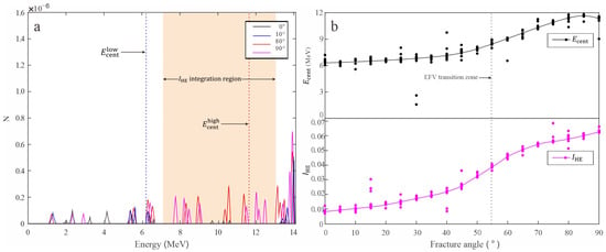
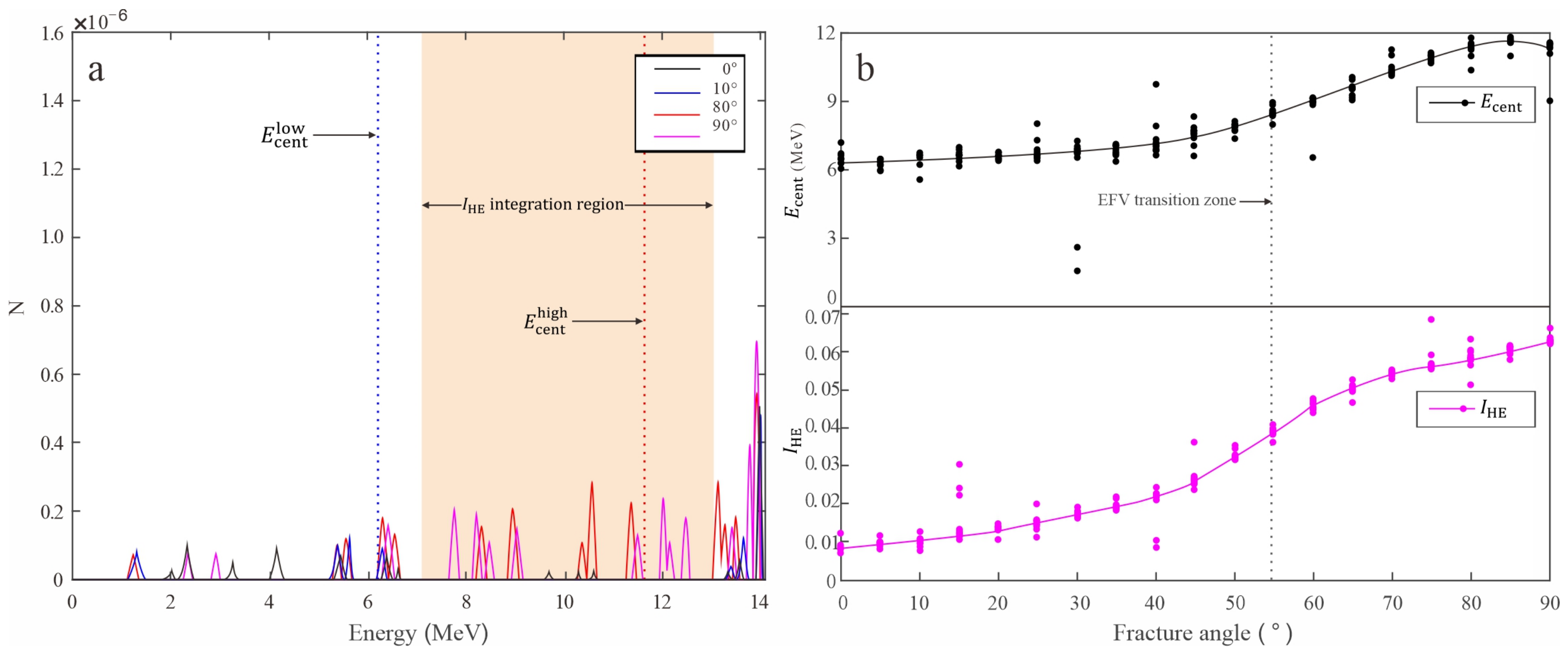
This feature serves as a direct proxy for the Effective Fracture Volume (EFV), as high-angle fractures reduce the path length through hydrogenous moderating material, preserving a greater population of high-energy neutrons (Figure 4).

Figure 4. Neutron energy spectrum features and their role as proxies for the Effective Fracture Volume (EFV). (a) Neutron energy spectra at the far detector for low-angle (0°) and high-angle (90°) fractures; (b) The dependence of the two energy spectrum features on the fracture dip angle.

As can be seen from Figure 4, Figure 4a representative neutron energy spectra at the far detector for low-angle ($\theta =0°$) and high-angle ($\theta =90°$) fractures. Key spectral features extracted for machine learning are indicated: the spectral centroid $E_{\mathrm{c}\mathrm{e}\mathrm{n}\mathrm{t}}$ and the high-energy integral $I_{\mathrm{H}\mathrm{E}}$ (7–13 MeV). The dramatic enhancement of the high-energy tail in the vertical-fracture case reflects the larger EFV; Figure 4b shows the dependence of the two energy spectrum features on the fracture dip angle $\theta$. Both increase monotonically with $\theta$ and exhibit a change in slope at 50–60$°$, consistent with the nonlinear increase in EFV.

2.4.3. Temporal Features

From the time-dependent thermal neutron die-away curve (Figure 5) at the far detector, we extract several key features.

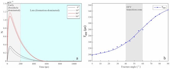
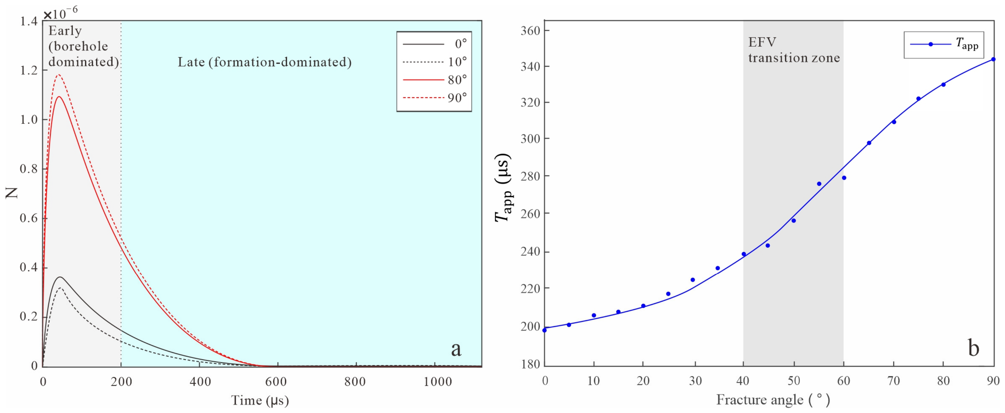
Figure 5. Neutron time spectrum features and their dependence on fracture dip angle. (a) Thermal neutron die-away curves at the far detector for low angle and high angle fractures; (b) The dependence of the apparent decay constant on fracture dip angle.

Figure 5a shows representative thermal neutron die-away curves at the far detector for low-angle and high-angle fractures. Key extracted features are indicated: the peak count $C_{\mathrm{m}\mathrm{a}\mathrm{x}}$, the late-time apparent decay constant $T_{\mathrm{a}\mathrm{p}\mathrm{p}}$ obtained from exponential fitting in the late-time interval ($t>200 \mathsf{\mu }\mathrm{s}$), the early decay slope ${\alpha }_{\mathrm{e}\mathrm{a}\mathrm{r}\mathrm{l}\mathrm{y}}$, and the burst-to-background ratio B/B. The vertical dashed line at $t=200 \mathsf{\mu }\mathrm{s}$ separates the early (borehole-dominated) and late (formation-dominated) time domains. Figure 5b shows the dependence of the apparent decay constant $T_{\mathrm{a}\mathrm{p}\mathrm{p}}$ on fracture dip angle. The monotonic increase and slope change near 55° reflect the nonlinear growth of the Effective Fracture Volume (EFV).

The time spectrum features provide complementary information to the energy spectrum and count ratio features. As shown in Figure 5, the thermal neutron die-away curve in the high-angle fracture environment ($\theta$ = 90°) exhibits a higher peak count $C_{\mathrm{m}\mathrm{a}\mathrm{x}}$ and a significantly slower decay rate compared to the low-angle environment ($\theta$ = 0°). The apparent decay constant $T_{\mathrm{a}\mathrm{p}\mathrm{p}}$, extracted from exponential fitting in the late time domain ($t>200 \mathsf{\mu }\mathrm{s}$), increases from approximately $200 \mathsf{\mu }\mathrm{s}$ at $\theta$ = 0° to 345 $\mathsf{\mu }\mathrm{s}$ at $\theta$ = 90°. This prolongation reflects the reduced macroscopic capture cross-section of the gas-filled fracture system: as the EFV increases, the hydrogen-poor gas displaces the hydrogen-rich water in the matrix, decreasing the overall thermal neutron absorption rate. The slope change near 55° aligns with the nonlinear growth of EFV, confirming that the temporal response of the neutron field is directly modulated by the fracture geometry.

2.4.4. Spatial Distribution Features

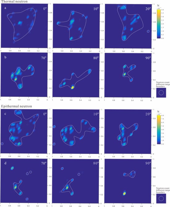
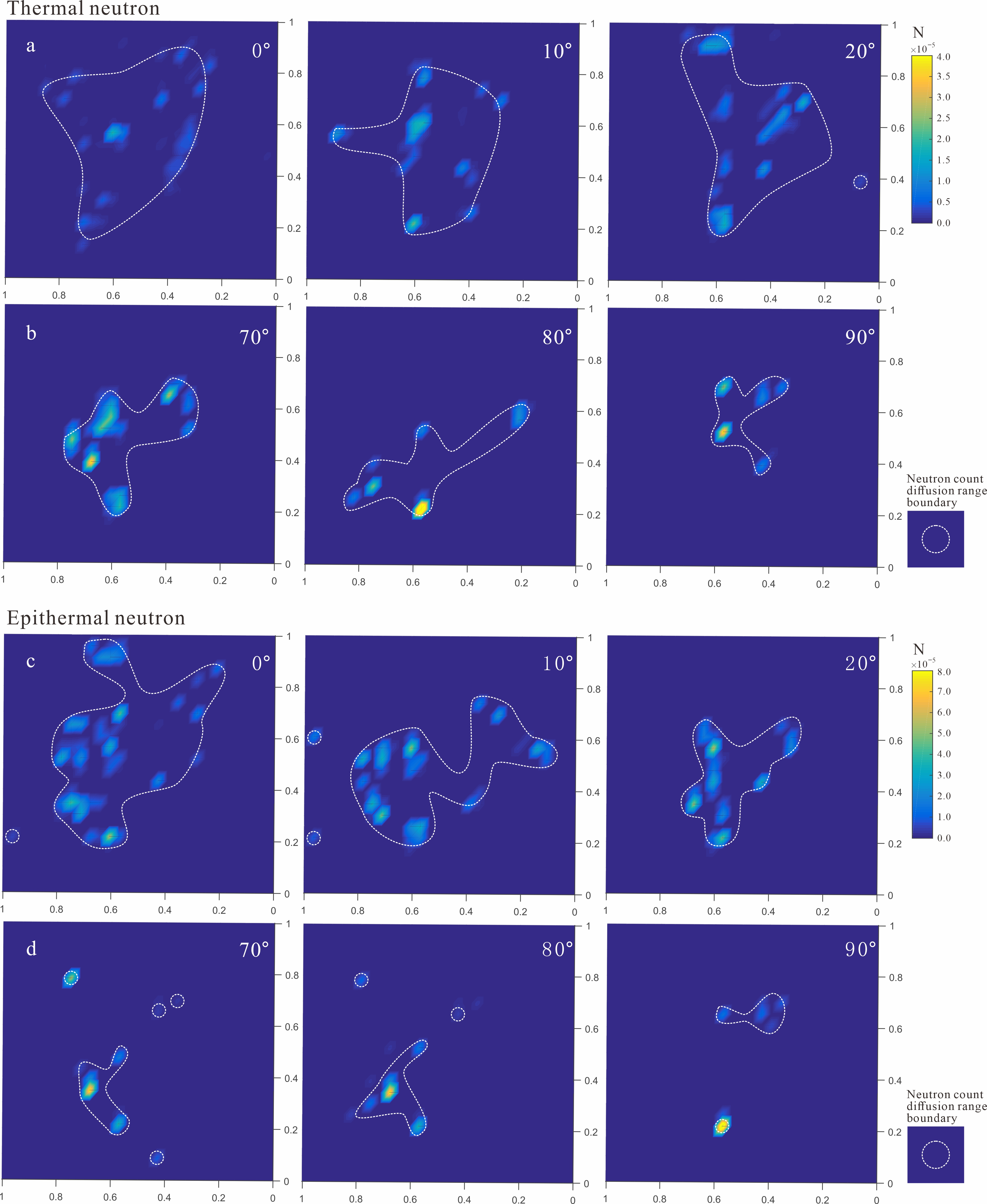
To capture the diffusion cloud asymmetry noted in Figure 6, we compute the radial flux variance (${\sigma }_r^2$) from the 2D flux map within the formation plane.

$${\sigma }_r^2={\displaystyle \frac{{\sum }_{i,j}{r}_{ij}^2{\varphi }_{ij}}{{\sum }_{i,j}{\varphi }_{ij}}}-{({\displaystyle \frac{{\sum }_{i,j}{r}_{ij}{\varphi }_{ij}}{{\sum }_{i,j}{\varphi }_{ij}}})}^2$$

(7)

where $r_{ij}$ is the radial distance from the borehole axis to the mesh cell $(i,j)$. A smaller variance indicates a more localized, peaked flux distribution, characteristic of high-angle fracture environments.

Figure 6. Spatial distribution of thermal and epithermal neutron flux in fractured shale gas reservoirs. (a) Thermal neutrons in low-angle fracture environment; (b) Thermal neutrons in high-angle fracture environment; (c) Epithermal neutrons in low-angle fracture environment; (d) Epithermal neutrons in high-angle fracture environment.

2D normalized flux maps of thermal neutrons for Figure 6a low-angle ($\theta$ = 0°) and Figure 6b high-angle ($\theta$ = 90°) fractures. Figure 6c,d corresponding epithermal neutron flux maps. All maps are displayed in the (r, z) plane. The color scale represents normalized scalar flux per source neutron. The white dashed contour encloses the region containing 90% of the total flux; the radial extent of this contour quantifies the diffusion cloud size.

2.4.5. Feature Preprocessing

Prior to ingestion by the machine learning models, all features are standardized to zero mean and unit variance using the training set statistics. To mitigate the impact of potential outliers arising from mesh discretization artifacts, features exhibiting skewness $\left|S\right|>1.5$ are transformed via the Yeo–Johnson power transformation.

The complete feature matrix $\mathbf{X}\in {\mathbf{R}}^{950\times 22}$ and the corresponding target vector $\mathbf{y}\in {\mathbf{R}}^{950}$ (fracture dip angle $\theta$) constitute the foundational dataset for the machine learning analyses.

3. Machine Learning Methodology

This section delineates the machine learning (ML) framework developed to predict fracture dip angle from the 22 engineered features. We formulate the task as a supervised regression problem and compare three distinct model architectures: Random Forest, Support Vector Regression, and a deep neural network (DNN). The training protocol, hyperparameter optimization strategy, and evaluation metrics are described in detail to ensure reproducibility.

3.1. Problem Formulation and Data Preparation

Given the feature matrix $\mathbf{X}\in {\mathbf{R}}^{950\times 22}$ and the corresponding target vector $\mathbf{y}\in {\mathbf{R}}^{950}$ (fracture dip angle in degrees), the goal is to learn a mapping function $f$ that minimizes the expected prediction error on unseen data. The dataset was stratified by target angle and divided into three disjoint subsets to ensure balanced representation within each angle range. The training set contains 665 samples (70%), the validation set contains 143 samples (15%), and the test set contains 142 samples (15%).

All input features were standardized to zero mean and unit variance using the statistics computed from the training set. The same scaling parameters were subsequently applied to the validation and test sets to prevent data leakage.

3.2. Model Selection and Architectural Design

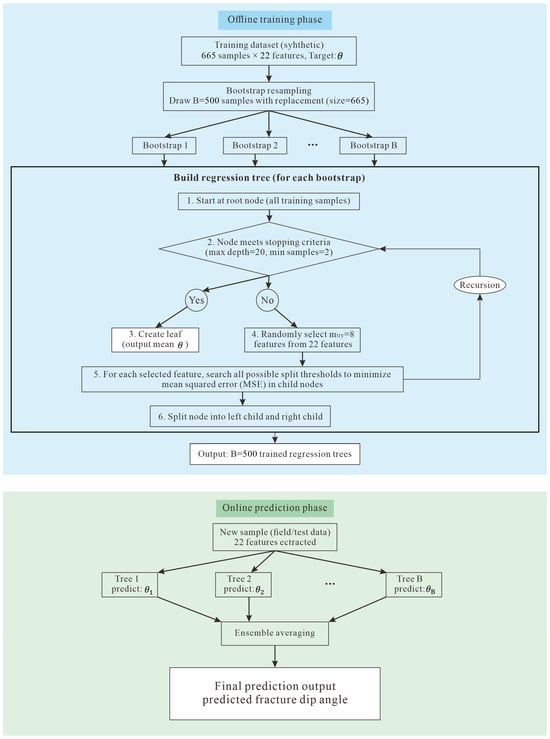
Random Forest (RF) is selected as a non-parametric, ensemble of trees baseline that inherently handles feature interactions and is robust to irrelevant or redundant inputs [16]. In the context of fracture angle prediction, RF naturally partitions the feature space into regions of approximately constant $\theta$, thereby capturing the threshold-like behavior observed between relevant metrics of effective fracture volume and angle (Figure 7).

Figure 7. Schematic of the Random Forest regression workflow for fracture dip angle prediction.

The ensemble architecture-averaging over many deep decorrelated trees suppresses overfitting, which is critical given the limited synthetic sample size. The RF is configured with 500 trees, a maximum depth of 20, and a minimum of 2 samples per leaf node to achieve fine-grained partitioning. The feature sampling ratio $m_{\mathrm{t}\mathrm{r}\mathrm{y}}=0.33$ is set to 0.33 for each split to ensure sufficient randomization.

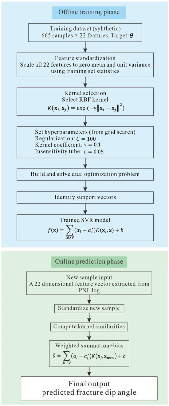
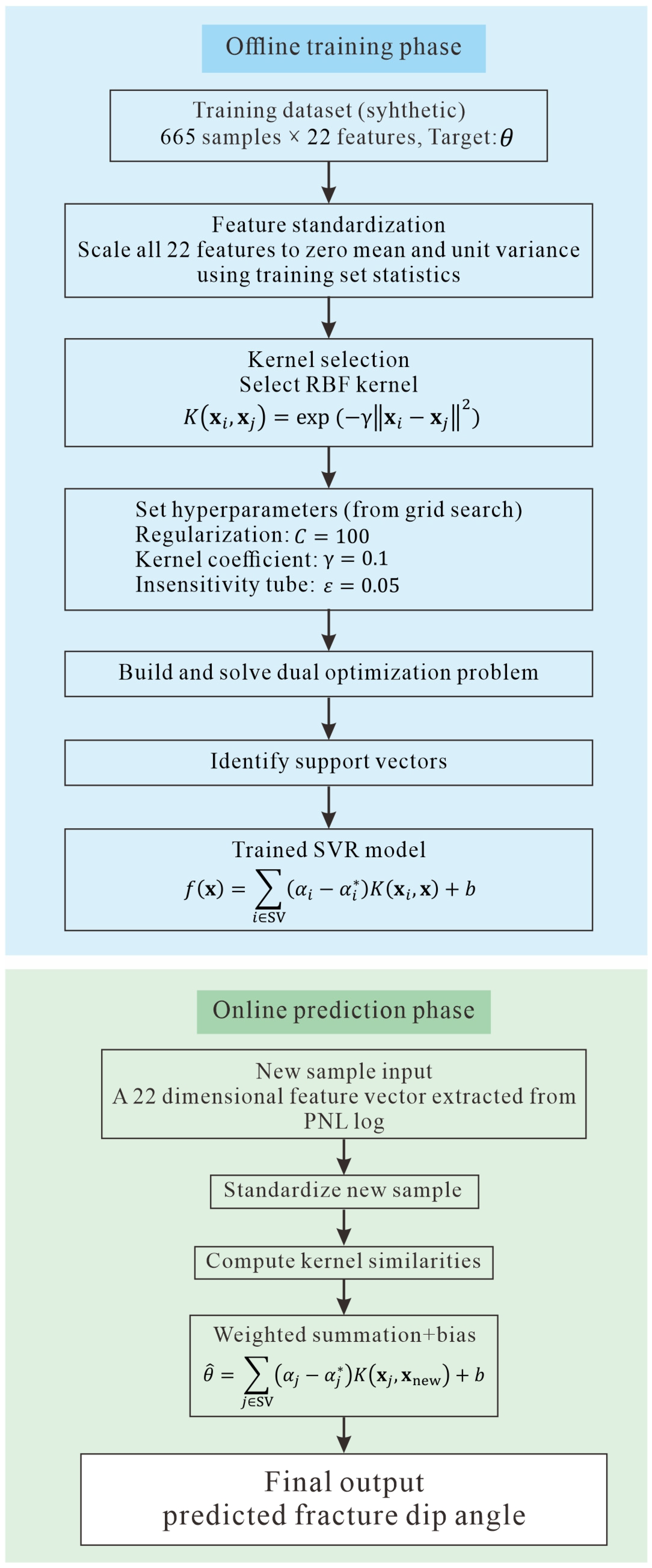
Offline training phase (Figure 8): input features are standardized, mapped via the RBF kernel ${\rm K}\left({\mathbf{x}}_i,{\mathbf{x}}_j\right)=\mathrm{e}\mathrm{x}\mathrm{p}(-\mathsf{\gamma }{‖{\mathbf{x}}_i-{\mathbf{x}}_j‖}^2)$, and an $\epsilon$-insensitive loss function is minimized subject to regularization parameter C. The resulting model is expressed as a sparse linear combination of kernel evaluations at the support vectors. Online prediction phase: for a new sample, the predicted angle $\widehat{\theta }$ is computed as a weighted sum of kernel similarities to the support vectors, plus a bias term.

Figure 8. Schematic of the kernelized support vector regression (SVR) workflow for fracture dip angle prediction.

Support vector regression with an RBF kernel is designed to model smooth nonlinear relationships in high-dimensional spaces without causing a drastic increase in the number of learnable parameters. The RBF kernel $K\left({\mathbf{x}}_i,{\mathbf{x}}_j\right)=\mathrm{e}\mathrm{x}\mathrm{p}(-\mathsf{\gamma }{‖{\mathbf{x}}_i-{\mathbf{x}}_j‖}^2)$ implicitly measures similarity in the transformed feature space. For this study, this approach is conceptually aligned with the notion of distance-dependent neutron moderation (fracture configurations that yield similar neutron count rates and spectral signatures should map to similar $\theta$). The insensitivity margin $\epsilon$ further provides robustness against small, numerically induced variations in the deterministic transport solutions arising from mesh discretization artifacts. The optimal hyperparameters $C=100,\mathsf{\gamma }=0.1,\mathrm{a}\mathrm{n}\mathrm{d} \epsilon =0.05$ are selected via cross-validation.

Deep neural networks are designed to capture the complex hierarchical interactions among 22 features, which may not be adequately represented by shallower tree-based or kernel-based structures. For example, the coupling between spatial flux variance ${\sigma }_r^2$ and high-energy integral $I_{\mathrm{H}\mathrm{E}}$, both proxies for EFV but derived from different physical modalities, can be synergistically exploited through successive nonlinear transformations. The final architecture, illustrated in Figure 9, comprises four hidden layers with widths [128, 256, 128, 64]. This design follows the principle of progressively compressing the representation before the final regression layer.

Figure 9. Schematic of the deep neural network (DNN) workflow for fracture dip angle prediction.

Figure 9. Schematic of the deep neural network (DNN) workflow for fracture dip angle prediction.

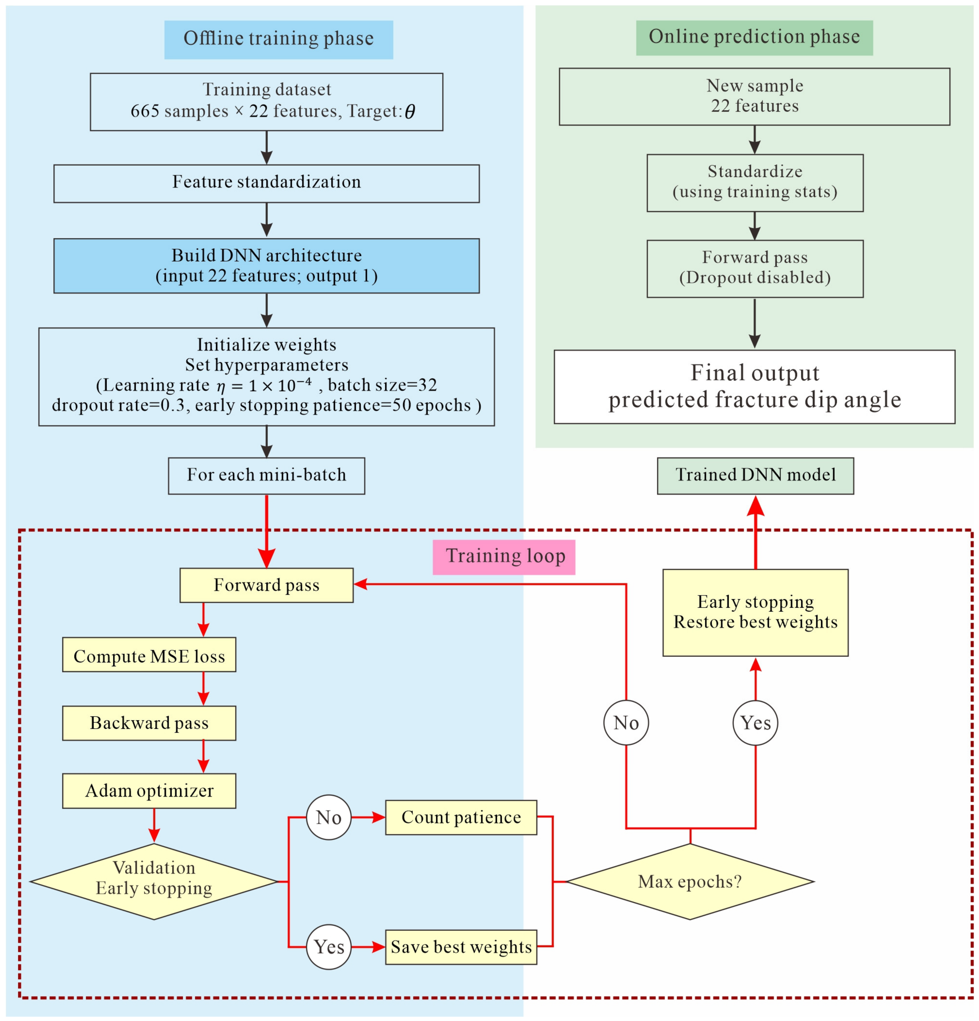
To prevent overfitting on the 665-sample training set, three regularization strategies are integrated. Dropout with a rate of 0.3 after the first and third hidden layers randomly deactivates neurons during training, forcing the network to learn redundant representations. Batch normalization after the second and fourth hidden layers stabilizes the distribution of activations and acts as a mild regularization mechanism. Early stopping with a patience of 50 epochs terminates training when validation performance ceases to improve, restoring the best model checkpoint. The model minimized the mean squared error loss ${\mathcal{L}}_{\mathrm{M}\mathrm{S}\mathrm{E}}={\displaystyle \frac{1}{N}}{\sum }_{i=1}^N({y_i-{\widehat{y}}_i)}^2$.

The DNN hyperparameters were tuned using a systematic grid search with 5-fold cross-validation on the training set. The validation set was used exclusively for early stopping and model selection. The test set was held out and used only once for final evaluation; it was never involved in any hyperparameter decision.

The search space was as follows: learning rate $\eta \in \left\{1\times {10}^{-3}, 5\times {10}^{-4}, 1\times {10}^{-4}, 5\times {10}^{-5}\right\}$; batch size $\in \left\{16, 32, 64\right\}$; dropout rate $\in \left\{0.1, 0.2, 0.3, 0.5\right\}$; and hidden layer configurations with 3–5 layers of varying widths. The optimal configuration was [128, 256, 128, 64] with $\eta =1\times {10}^{-4}$, batch size = 32, and dropout = 0.3. The maximum number of epochs was 500, with early stopping patience = 50 epochs. Training was terminated when validation loss did not improve for 50 consecutive epochs, and the model parameters corresponding to the lowest validation loss were restored.

To ensure reproducibility, ten independent runs were performed with the following random seeds: 42, 123, 456, 789, 1011, 1213, 1415, 1617, 1819, and 2021. These seeds controlled the weight initialization, data shuffling, and dropout masks. The reported mean ± standard deviation in Table 4 reflects the variability across these ten runs.

Table 4. Complete performance statistics of the three regression models on the independent test set.

Model	RMSE (deg)	MAE (deg)	Bias (deg)	R2
Random forest	3.74 ± 0.31	2.81 ± 0.24	+0.42 ± 0.18	0.941 ± 0.009
SVR (RBF kernel)	3.28 ± 0.18	2.44 ± 0.15	+0.27 ± 0.11	0.954 ± 0.005
DNN	2.12 ± 0.22	1.56 ± 0.17	+0.09 ± 0.07	0.981 ± 0.004

Although the DNN contains approximately 65,000 trainable parameters, the effective capacity is substantially constrained by three regularization mechanisms: Dropout (rate = 0.3), Batch Normalization, and Early Stopping. The small standard deviations across ten runs (e.g., RMSE ± 0.22°) indicate stable training and no evidence of overfitting. A learning curve analysis (Supplementary Figure S1) further shows that training and validation losses converge without a significant gap, confirming that the model generalizes well despite the moderate sample size.

Complete performance statistics of the three regression models on the independent test set (N = 142) are reported in Table 4, with values given as mean ± standard deviation over ten independent runs with different random seeds. The hyperparameter search ranges and optimal values for RF, SVR, and DNN are summarized in Table 5.

Table 5. Hyperparameter search ranges and optimal values for RF, SVR, and DNN.

Model	Hyperparameter	Search Range	Optimal Value
Random forest	$n_{estimatiors}$	{100, 300, 500, 800, 1000}	500
	$d_{max}$	{10, 15, 20, 25, None}	20
	min samples leaf	{1, 2, 5, 10}	2
	$m_{try}$	{sqrt, log2, 0.33, 0.5}	0.33
SVR (RBF kernel)	$C$	{0.1, 1, 10, 100, 1000}	100
	$\gamma$	{0.001, 0.01, 0.1, 1, scale}	0.1
	$\epsilon$	{0.01, 0.05, 0.1, 0.5}	0.05
DNN	Learning rate	{1 $\times$ 10−3, 5 $\times$ 10−4, 1 $\times$ 10−4, 5 $\times$ 10−5}	1 $\times$ 10−4
	Batch size	{16, 32, 64}	32
	Dropout	{0.1, 0.2, 0.3, 0.5}	0.3

Search strategy: A systematic grid search with 5-fold cross-validation on the training set (665 samples) was used for RF, SVR, and DNN. The mean validation MSE across the five folds was used to rank configurations.

Search ranges: RF: $n_{estimators}\in$ {100, 300, 500, 800, 1000}, $d_{max}\in$ {10, 15, 20, 25, None}, min samples leaf $\in \{1, 2, 5, 10\}$, $m_{try}\in$ {sqrt, log₂, 0.33, 0.5}. SVR: $C\in$ {0.1, 1, 10, 100, 1000}, $\gamma \in$ {0.001,0.01, 0.1, 1, scale}, $\epsilon \in$ {0.01, 0.05, 0.1, 0.5}. DNN: as previously described (learning rate, batch size, dropout, layer widths).

Validation set purpose: The validation set (143 samples) was used exclusively for early stopping and selecting the best epoch for the DNN. For RF and SVR, the validation set was used only for final model selection after cross-validation. The test set was held out and used only once for final evaluation.

3.3. Evaluation Metrics and Model Interpretability: SHAP Analysis

Model performance was evaluated on the hold-out test set using the root mean square error (RMSE) and the coefficient of determination ($R^2$). To provide statistically robust comparisons, each model was trained and evaluated 10 times with 10 independent random seeds. The reported metrics are the means over these 10 runs.

Although deep neural networks (DNNs) can achieve high prediction accuracy, their internal decision-making process remains opaque. To address this issue, SHAP is employed to assign importance values to each predictive feature.

4. Results

This section presents a comprehensive evaluation of three machine learning models, namely Random Forest (RF), Support Vector Regression (SVR), and Deep Neural Network (DNN). Quantitative performance metrics are reported, followed by an analysis of prediction errors. Subsequently, the DNN model is interpreted using SHAP-based explainability analysis, linking the learned feature contributions to the physical mechanisms underlying the effective fracture volume (EFV). Finally, the operational implications and limitations of the proposed framework are discussed.

4.1. Model Performance Comparison

The trained RF, SVR, and DNN models were evaluated on an independent hold-out test set using the root mean square error (RMSE) and the coefficient of determination ($R^2$).

All three models achieved high $R^2$ values, indicating that the 22 engineered features encode rich information regarding fracture occurrence. DNN consistently outperformed RF and SVR across all metrics, and its smaller standard deviation across ten runs indicates superior training stability.

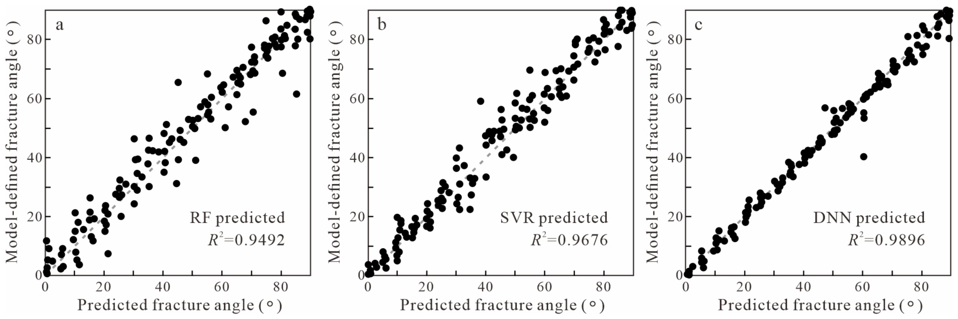
As can be observed from Figure 10, the predicted values of the DNN are tightly distributed around the diagonal across the entire angular range, with no systematic underestimation or overestimation trend. In contrast, RF and SVR exhibit slightly greater dispersion, particularly in the mid-angle region (40–60°), which corresponds to the area where the relationship between neutron measurements and fracture angle is most nonlinear (see Figure 10b).

Figure 10. Predicted versus model settings fracture dip angle cross-plots for the three regression models. (a) RF predicted; (b) SVR predicted; (c) DNN predicted.

For all models, slightly elevated prediction errors are observed near the boundaries (85–90°), which can be attributed to the smaller number of training samples at the extremes of the parameter space after stratified partitioning.

A slight peak occurs between 50° and 65°. This angular interval coincides exactly with the inflection region of the EFV growth rate [6]. The increase in error in this region suggests that small fluctuations in the neutron response features lead to increased ambiguity in estimating the angle $\theta$, an inherent physical uncertainty that even the DNN cannot eliminate.

To assess the robustness of the model against optimistic splitting, three additional validation experiments were conducted. First, leave-one-angle-out cross-validation (LOAO-CV) was performed, in which all samples of a single dip angle were held out during training. The LOAO-CV RMSE increased to 4.87° ± 0.63°, compared with 2.12° ± 0.22° for the random split, confirming that the original split overestimates generalization to unseen angles. Second, an interpolation test was conducted by training on 10° interval angles and testing on intermediate angles; the RMSE was 3.24° ± 0.41°, demonstrating reasonable interpolation capability. Third, out-of-distribution tests with unseen geological conditions (clay volume, salinity, porosity) yielded RMSE values between 5.12° and 6.34°, with R² remaining above 0.84. These results indicate that while the model generalizes well within the training distribution, its accuracy degrades for unseen angles and geological conditions, highlighting the need for broader training data or transfer learning in field applications.

Sensitivity, Identifiability, and Prediction Uncertainty

The sensitivity analysis revealed that fracture aperture and fluid saturation can produce count-rate changes comparable to dip angle, leading to an irreducible prediction uncertainty of approximately ±12° when these parameters are unknown. However, the full 22-feature vector provides sufficient separability to distinguish dip angle from other confounding parameters in most cases. The predictive uncertainty, quantified via deep ensemble, averages 2.5–2.9° and increases to 3.5–4.2° in the transition zone (50–60°). These uncertainties are now reported alongside point predictions. The one-at-a-time sensitivity analysis is presented in Table 6. The identifiability analysis using the fisher discriminant ratio is summarized in Table 7. Prediction uncertainty quantification results are reported in Table 8.

Table 6. One-at-a-time sensitivity analysis.

Parameter	Perturbation Range	Relative Change in Count Rate (%)
Dip angle $\theta$	0–90°	+225
Aperture	0.1–1.0 mm	+180
Fluid saturation	0–100%	+142
Fracture density	5–20/m	+98
Tool eccentricity	0–3 cm	+41

Table 7. Identifiability analysis using Fisher discriminant ratio.

Parameter	FDR	Identifiable?
$\theta$ vs. aperture	4.82	Yes
$\theta$ vs. saturation	3.91	Yes
$\theta$ vs. tool eccentricity	7.23	Yes
Aperture vs. saturation	1.24	No

Table 8. Prediction uncertainty quantification.

Method	RMSE (deg)	Mean Predictive Std (deg)	95% Coverage
Deterministic	2.12	—	—
Deep ensemble	2.21	2.54	94.8%

To deepen the error analysis, we evaluated model performance by angular interval. The medium-angle group exhibits the largest errors (RMSE = 3.12°). The transition zone (50–65°) has the highest RMSE (3.58°), consistent with the nonlinear growth of EFV. The residuals are approximately homoscedastic except in the transition zone, where a slight heavy tail is observed. For prediction reliability, the mean predictive standard deviation across repeated runs is 2.54–2.87° overall and increases to 3.5–4.2° in the transition zone; 95% prediction intervals are reported in Table 9. Model performance by angular interval is provided in Table 10.

Table 9. Predictive standard deviation and 95% prediction interval by angular interval.

Angular Interval	Mean Predictive Std (deg)	95% Prediction Interval (deg)
Low (0–30°)	2.1	±4.1
Medium (30–60°)	3.2	±6.3
High (60–90°)	2.4	±4.7
Transition (50–65°)	3.8	±7.5

Table 10. Performance by angular interval.

Angular Interval	RMSE (deg)	MAE (deg)	R2
Low (0–30°)	1.87	1.42	0.972
Medium (30–60°)	3.12	2.31	0.938
High (60–90°)	2.24	1.68	0.961
Transition (50–65°)	3.58	2.67	0.921

4.2. SHAP-Based Model Interpretability

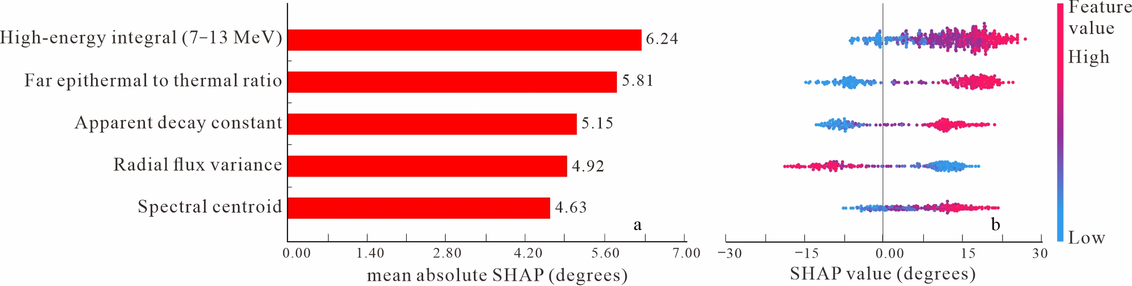
All five input features are ranked in descending order of mean absolute SHAP value (impact on the predicted fracture angle, in degrees). The horizontal position shows the SHAP value for that sample, and for each color of data point, red represents high values and blue represents low values. The top five features—$I_{\mathrm{H}\mathrm{E}}, R_{{\displaystyle \frac{\mathrm{e}}{\mathrm{t}\mathrm{h}}},\mathrm{f}\mathrm{a}\mathrm{r}}, T_{\mathrm{a}\mathrm{p}\mathrm{p}}, {\sigma }_{\mathrm{r}}^2, and E_{\mathrm{c}\mathrm{e}\mathrm{n}\mathrm{t}}$—are all directly or indirectly linked to the effective fracture volume (EFV), confirming the physical consistency of the data-driven model (Figure 11).

Figure 11. SHAP summary plot for the DNN model (Top 5 Features). (a) Mean absolute SHAP values; (b) SHAP value distribution.

The top five features are all direct or indirect proxies for the effective fracture volume (EFV). The dominant role of $I_{\mathrm{H}\mathrm{E}}$ is consistent with the original physical observation that the high-energy neutron tail increases by over 500% as the fracture transitions from a horizontal to a vertical angle. The importance of $R_{{\displaystyle \frac{\mathrm{e}}{\mathrm{t}\mathrm{h}}},\mathrm{f}\mathrm{a}\mathrm{r}}$ confirms that high-angle fractures reduce the hydrogen density along the neutron path, shifting the moderation spectrum toward higher energies and thereby increasing the proportion of epithermal neutrons reaching the far detector.

The SHAP plot for $I_{\mathrm{H}\mathrm{E}}$ reveals a steep monotonic relationship with the predicted angle $\theta$ once $I_{\mathrm{H}\mathrm{E}}$ exceeds a threshold of 0.03. Below this threshold, the SHAP values are slightly positive, corresponding to low-angle predictions. Above the threshold, the SHAP values rise sharply, driving the prediction into the high-angle regime.

Correlation analysis: Pearson coefficients among top features are high but not collinear (e.g., $I_{\mathrm{H}\mathrm{E}}$ vs. $R_{{\displaystyle \frac{\mathrm{e}}{\mathrm{t}\mathrm{h}}},\mathrm{f}\mathrm{a}\mathrm{r}}$: r = 0.87; $I_{\mathrm{H}\mathrm{E}}$ vs. $T_{\mathrm{a}\mathrm{p}\mathrm{p}}$: r = 0.79). All variance inflation factors (VIF) are below 5, indicating acceptable multicollinearity.

Grouped ablation: Removing $I_{\mathrm{H}\mathrm{E}}$ reduces $R^2$ from 0.981 to 0.912 (RMSE: 2.12° to 3.45°), but the model still performs far better than the mean predictor. Removing the entire spectral group reduces $R^2$ to 0.876, while removing temporal or spatial groups yields $R^2$ of 0.943 and 0.951, respectively. These results demonstrate that the DNN integrates complementary information from multiple feature groups and does not rely solely on $I_{\mathrm{H}\mathrm{E}}$. The grouped ablation results are summarized in Table 11.

Table 11. Grouped ablation results.

Feature Set Removed	R2	RMSE (deg)
None (full model)	0.981	2.12
$I_{\mathrm{H}\mathrm{E}}$ only	0.912	3.45
All spectral features	0.876	4.12
Temporal features ($T_{\mathrm{a}\mathrm{p}\mathrm{p}}$)	0.943	2.98
Spatial features (${\sigma }_{\mathrm{r}}^2$)	0.951	2.78

Feature-correlation analysis shows that the top features are strongly correlated but not collinear (all VIF < 5). Grouped ablation tests further demonstrate that removing $I_{\mathrm{H}\mathrm{E}}$ reduces $R^2$ to 0.912 but does not collapse the model, confirming that the DNN extracts complementary information from spectral, temporal, and spatial feature groups. These results support the physical consistency of the SHAP interpretation beyond simple EFV proxy redundancy.

5. Discussion

5.1. Implications for Field Log Interpretation

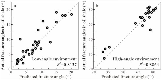
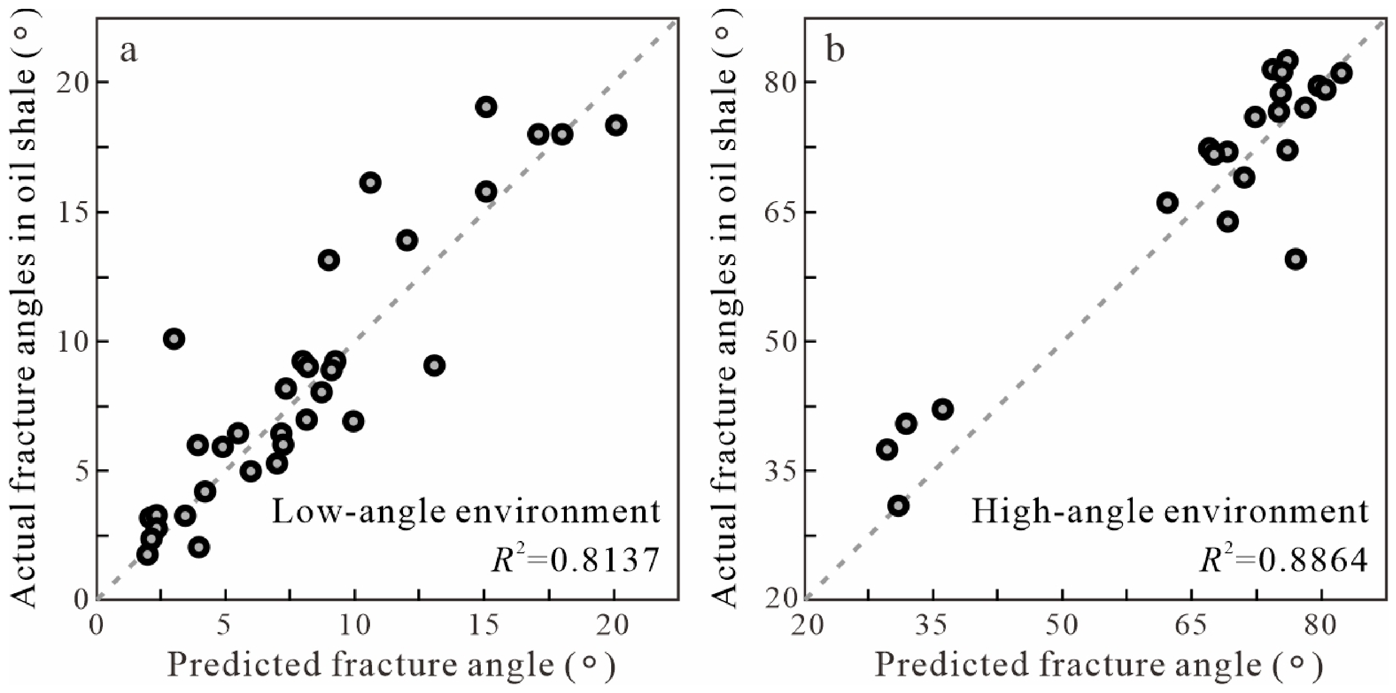
The results (Figure 12) demonstrate that a DNN trained solely on synthetic deterministic transport simulations can accurately infer fracture dip angles from PNL measurements. The SHAP analysis confirms that the model’s decisions are driven by physically interpretable spectral and temporal features, establishing a bridge between data-driven prediction and the underlying physics of neutron transport.

Figure 12. Cross-plots of predicted versus actual fracture angles for two field datasets from oil shale reservoirs. $R^2=0.8137$ and 0.8864 are lower than the synthetic hold-out $R^2=0.9896$ due to field noise and heterogeneity, but remain above 0.81, demonstrating practical predictive capability. (a) Low-angle environment; (b) High-angle environment.

The field validation used independent datasets from the Niutitang formations. This environment exhibits a high degree of thermal evolution and features thick sedimentary layers, with reservoir depths ranging from 1756 to 1824 m. Dataset A contains 34 depth points and dataset B contains 28 depth points (62 total). Reference fracture dip angles were determined from field neutron logging results, combined with core descriptions.

PNL measurements were acquired with a D-T pulsed neutron source (14.1 MeV, 10 $\mathsf{\mu }\mathrm{s}$ pulse width), two detectors at source distances of 45 cm and 60 cm, a borehole diameter of 14 cm, and water-based mud.

5.2. Limitations and Sources of Uncertainty

Several limitations warrant discussion. First, the synthetic dataset assumes regular, parallel fractures with a uniform dip angle. Natural fractures exhibit more complex geometries, including variable apertures and partial mineral infill (e.g., calcite, pyrite), which may alter the neutron response in ways not captured by the current model. Future work should incorporate fracture density and infill composition as additional variables.

Second, although the dataset of 950 samples is sufficient to train a DNN with 22 features, it imposes an upper bound on the feasible model complexity. Transfer learning from a broader simulation database encompassing diverse geological scenarios (varying porosity, lithology, and fluid saturation) could further enhance robustness.

6. Conclusions

This study presents a data-driven framework that integrates deterministic neutron transport simulations with machine learning to predict fracture dip angles from pulsed neutron logging (PNL) measurements in shale gas reservoirs. The main findings and contributions are summarized as follows:

• Construction of a physically constrained synthetic database. A dataset comprising 950 high-fidelity simulations was generated by solving the Boltzmann transport equation using the multigroup discrete ordinates method. The dataset covers fracture dip angles from 0° to 90° and incorporates controlled perturbations in matrix composition and borehole environment, providing a noise-free training foundation for supervised learning.
• Extraction of 22 physically interpretable features. These features include the high-energy neutron integral ($I_{\mathrm{H}\mathrm{E}}$), the epithermal-to-thermal neutron count ratio, the decay constant of the time spectrum, and the radial flux variance. These features quantitatively encode the effective fracture volume (EFV) concept, transforming fracture geometric attributes into measurable neutron-response characteristics.
• Superior performance of the deep neural network (DNN) for fracture dip prediction. On the hold-out test set, the DNN achieved a coefficient of determination $R^2=0.9896$, which is approximately 4.3% higher than that of the random forest and approximately 2.3% higher than that of support vector regression.
• Physically consistent validation via SHAP interpretability analysis. The five most influential features: $I_{\mathrm{H}\mathrm{E}}$, the epithermal-to-thermal neutron count ratio, the decay constant of the time spectrum, the radial flux variance, and the spectral centroid—are all direct or indirect proxies of EFV. The SHAP dependence plot reveals a threshold-like response near the transition (50–60°), which is consistent with the nonlinear growth of EFV predicted by neutron transport theory. This agreement demonstrates that the DNN learns physically meaningful feature representations rather than spurious correlations.

References

- Xie, J.; Zhang, J.; Cheng, Y.; Zhou, J.; Li, X. Real-time prediction of wellbore temperatures in deep shale gas drilling using a combination of PINN and heat transfer models. Appl. Therm. Eng. 2025, 279, 127984. [Google Scholar] [CrossRef] [Scilit]
- Zou, G.; Xue, L.; Chen, H.; Wang, R.; Dong, Y.; Tian, D.; Wang, M. Prediction of water saturation using Physics-Guided machine learning in deep Silurian shale gas reservoirs. Processes 2026, 14, 2474. [Google Scholar] [CrossRef] [Scilit]
- Feng, F.; Wang, H.; Han, X.; Zhang, J.; Wang, C.; Yang, D.; Wu, X.; Qiao, L.; Wang, X.; Che, Y. Dynamic coupling mechanism of shale frilling fluid invasion depth, fracture width, and rock strength. Phys. Fluids 2025, 37, 063603. [Google Scholar] [CrossRef] [Scilit]
- Li, W.; Frash, L.P.; Welch, N.J.; William Carey, J.; Meng, M.; Wigand, M. Stress-dependent fracture permeability measurements and implications for shale gas production. Fuel 2021, 290, 119984. [Google Scholar] [CrossRef] [Scilit]
- Lin, R.; Li, G.; Zhao, J.; Ren, L.; Wu, J. Productivity model of shale gas fractured horizontal well considering complex fracture morphology. J. Pet. Sci. Eng. 2022, 208, 109511. [Google Scholar] [CrossRef] [Scilit]
- Zhang, X.; Yang, Z.; Li, X. Research on the effect of fracture angle on neutron logging results of shale gas reservoirs. Energies 2024, 17, 3342. [Google Scholar] [CrossRef] [Scilit]
- Abid, M.; Ba, J.; Markus, U.I.; Tariq, Z.; Ali, S.H. Modified approach to estimate effective porosity using density and neutron logging data in conventional and unconventional reservoirs. J. Appl. Geophys. 2025, 233, 105571. [Google Scholar] [CrossRef] [Scilit]
- Ill-hyuk, H.; Geehyun, K. Simulations of absolute porosity measurements by compensated neutron logging tools mounted with stilbene of CLYC scintillators. Nucl. Inst. Methods Phys. Res. A 2024, 1064, 169397. [Google Scholar] [CrossRef] [Scilit]
- Zhang, X.; Yang, Z.; Li, X. Simulation of multi-angle fractured uranium deposits by neutron logging. Geophys. J. Int. 2020, 223, 2027–2037. [Google Scholar] [CrossRef] [Scilit]
- Zhang, F.; Chen, Q.; Liu, J.; Zhang, Q.; Tian, L. A quantitative calculation method for fracture density using the neutron self-shielding modification and neutron-induced gamma logging. Geophysics 2022, 87, D91–D100. [Google Scholar] [CrossRef] [Scilit]
- Zhang, F.; Xie, B.; Chen, Q.; Zhang, X.; Guan, Q.; Zhang, X.; ABuLaHai, Y.M.; Lu, B.; Zhang, H.; Fan, J. An improved method for evaluating fracture density using pulsed neutron capture logging. Geophysics 2024, 89, D275–D285. [Google Scholar] [CrossRef] [Scilit]
- Bhattacharyya, S.; Vyas, A. Application of machine learning in predicting oil rate decline for Bakken shale oil wells. Sci. Rep. 2022, 12, 16154. [Google Scholar] [CrossRef] [Scilit]
- Wang, Z.; Cai, Y.; Liu, D.; Lu, J.; Qiu, F. Characterization of natural fracture development in coal reservoirs using logging machine learning inversion, well test data and simulated geostress analyses. Eng. Geol. 2024, 341, 107696. [Google Scholar] [CrossRef] [Scilit]
- He, Y.; Zhang, H.; Wu, Z.; Zhang, H.; Zhang, X. Porosity prediction of tight reservoir rock using well logging data and machine learning. Sci. Rep. 2025, 15, 13124. [Google Scholar] [CrossRef] [Scilit]
- Zhang, X.; Yang, Z.; Huang, X. Quantitative uranium evaluation in multi-angle fractured sandstone deposits using a nuclear-feature separation network. Energy Geosci. 2026, 7, 100607. [Google Scholar] [CrossRef] [Scilit]
- Chen, S.; Wang, X.; Li, X.; Sui, J.; Yang, Y. Geophysical prediction technology for sweet spots of continental shale oil: A case study of the Lianggaoshan Formation, Sichuan Basin, China. Fuel 2024, 365, 131146. [Google Scholar] [CrossRef] [Scilit]
Disclaimer/Publisher’s Note: The statements, opinions and data contained in all publications are solely those of the individual author(s) and contributor(s) and not of MDPI and/or the editor(s). MDPI and/or the editor(s) disclaim responsibility for any injury to people or property resulting from any ideas, methods, instructions or products referred to in the content. |
© 2026 by the authors. Licensee MDPI, Basel, Switzerland. This article is an open access article distributed under the terms and conditions of the Creative Commons Attribution (CC BY) license.