PGNN-Based Harmonic Source Localization in Distribution Networks

Abstract

Accurate localization and quantification of multiple harmonic sources from limited synchronized measurements remain challenging in distribution networks. To address measurement noise, limited phasor measurement unit (PMU) deployment, and insufficient physical consistency in purely data-driven models, this paper proposes a physics-guided neural network (PGNN) incorporating bus-injection-to-branch-current (BIBC) constraints. The method combines the branch harmonic-current phasors available under the PMU observability configuration with a minimum-norm nodal-current prior obtained using the pseudoinverse of the corresponding observable BIBC submatrix. A shared convolutional feature extractor with classification and regression heads jointly estimates source locations and nodal harmonic injection currents. A BIBC-based branch-current consistency term penalizes discrepancies between reconstructed and available branch currents. Simulations on the modified IEEE 13-bus and modified IEEE 33-bus systems demonstrate that, under complete branch-current observability and a nominal noise level of 5%, PGNN achieves higher exact-match accuracy (EM) and micro-averaged F1-scores than the convolutional neural network (CNN), fully connected neural network (FCNN), and graph convolutional network (GCN) baselines for the 3rd, 5th, 7th, and 11th harmonics. Under these conditions, PGNN also yields lower current-magnitude percentage errors and phase-angle errors relative to the BIBC-derived reference. Further tests using third-harmonic data from the modified IEEE 33-bus system characterize PGNN performance under 0–20% noise, reduced training-set sizes, and selected reduced-PMU configurations. These results demonstrate the effectiveness of integrating BIBC-based physical priors with data-driven learning for joint harmonic source localization and nodal harmonic injection-current estimation on the two simulated radial distribution systems considered in this study.

1. Introduction

Amid the global energy transition and efforts to achieve carbon peaking and carbon neutrality goals, distributed energy resources (DERs), such as photovoltaic energy and wind generation, are increasingly being integrated into distribution systems alongside numerous nonlinear power electronic devices [1]. This development has profoundly reshaped the steady-state power quality characteristics of distribution networks, leading to increasingly severe harmonic pollution that compromises their secure and stable operation [2]. Specifically, harmonics interact with the inherent high-frequency impedance characteristics of distribution networks, potentially exciting complex resonance phenomena. These interactions can increase network losses, accelerate equipment aging, and interfere with the operation of capacitor banks and protection devices [3,4]. As DER penetration increases, harmonic sources may occur simultaneously at multiple buses and exhibit varying magnitudes and phase angles under different operating conditions. These characteristics challenge conventional monitoring approaches and complicate coordinated multi-source localization across the network [5]. Existing harmonic source localization methods used to address these issues can be broadly classified into three categories: equivalent circuit model-based methods, model-driven harmonic state estimation (HSE), and purely data-driven approaches.

Early studies on harmonic source localization relied heavily on analytical approaches and equivalent circuit models. These methods typically divide the network at the point of common coupling (PCC) into the system side and the user side. Harmonic sources are then identified by examining the direction of active or reactive power flow, critical impedance, or voltage–current ratios derived from measured voltage and current signals [6,7]. Although these single-point evaluation methods are straightforward to implement, many rely on simplifying assumptions about harmonic power-flow direction and operating conditions. These assumptions may be violated when multiple harmonic sources operate concurrently or under reverse-power-flow conditions, reducing localization reliability and limiting coordinated multi-bus analysis across the network.

HSE has been widely adopted to overcome the limitations of single-point evaluation methods. By combining power system topology with nodal measurements, HSE formulates harmonic source localization as a global inverse problem [8]. Various mathematical techniques have been proposed to address underdetermined HSE caused by insufficient measurement coverage in practical distribution networks. One category focuses on sparse reconstruction and signal recovery, including compressed sensing, orthogonal matching pursuit (OMP), and sparse Bayesian learning (SBL) [9,10,11]. Another uses blind source separation and advanced optimization algorithms to improve noise resistance, including fast independent component analysis combined with joint entropy, adaptive particle swarm optimization, and robust models based on the least median of squares (LMedS) criterion [12,13,14,15,16]. Although these methods have enriched the theoretical framework of HSE, their practical performance depends on sufficiently accurate network topology, line parameters, synchronized phasor measurements, and measurement redundancy. The inverse estimation process may amplify time-synchronization errors and line-parameter deviations, degrading localization accuracy or numerical stability. In addition, the cost of distribution-level PMUs can limit measurement coverage in practical distribution networks.

Purely data-driven deep learning approaches have been widely applied to harmonic source localization in recent years to reduce reliance on highly detailed physical models and extensive synchronized measurements. Unlike HSE-based methods, data-driven models do not require explicit construction of complex admittance matrices. Various deep learning architectures, including CNNs, generative adversarial networks (GANs), and GCNs, have been introduced for efficient end-to-end harmonic source localization [17]. However, these black-box approaches have limitations in generalization. Their performance depends heavily on large, high-quality labeled datasets covering diverse topology configurations and operating conditions, whereas high-frequency harmonic measurements in practical distribution networks are extremely sparse [18,19]. More importantly, although some studies have used graph neural network-based architectures to improve adaptability to topology variations, many of these approaches do not explicitly encode network-physics relationships such as Kirchhoff’s current law. Changes in electrical coupling may therefore substantially degrade model generalization, and the resulting predictions may violate Kirchhoff’s current law or network-topology constraints. The lack of physical interpretability also hinders engineering validation and fault diagnosis.

Physics-informed and physics-guided neural networks provide a general framework for incorporating known physical relationships into data-driven learning [20]. Depending on the problem, physical knowledge can be incorporated through the network architecture, input features, or additional loss terms. At the network-modeling level adopted here, steady-state harmonic currents in a radial distribution network are described by a discrete BIBC mapping derived from Kirchhoff’s current law rather than by continuous partial differential equation residuals [21,22,23]. Accordingly, this study incorporates BIBC-based information into both the hybrid input and the loss function to encourage consistency between predicted nodal harmonic injection currents and available branch-current measurements.

Shuai et al. [24] formulated harmonic source localization as node-wise binary classification using minute-averaged RMS values of harmonic voltages and currents. Their reconstructed DGCRN combines an impedance-derived electrical adjacency matrix with a dynamically learned topology to represent network uncertainty. Ngo et al. [25] combined Kalman estimation based on a branch-current model with graph learning to estimate bus-voltage magnitudes and phase angles. Mack et al. [26] used neural-network pruning based on grid connectivity to estimate nodal harmonic-voltage phasors from sparse synchronized voltage measurements. These studies incorporate electrical-network knowledge in different ways. Their prediction targets and mechanisms for incorporating physical information differ from those considered here.

Against this background, we develop a BIBC-guided current-domain framework for joint harmonic source localization and nodal harmonic injection-current estimation in radial distribution networks. The framework uses available branch-current phasors and the nodal-current prior obtained through the BIBC pseudoinverse as hybrid inputs. A shared feature extractor supports source-bus classification and current-phasor regression, while an observable-branch consistency loss regularizes the reconstructed branch currents against the available measurements. Table 1 summarizes the methodological distinctions and measurement assumptions. The contribution lies in this task-specific formulation and integration, rather than in the general introduction of physics-guided learning.

Table 1. Comparison of the proposed framework with closely related learning-based methods.

Method	Physical/Topological Information	Input Construction	Prediction Output	Measurement and Structural Assumptions
DGCRN	Electrical-distance static graph fused with learned dynamic graph; binary-classification loss	Minute-averaged harmonic voltage and current RMS values	Node-wise source probabilities and binary source labels	Selected-bus PQMD measurements; initial electrical graph combined with learned dynamic topology
GNN	Branch-current-model Kalman estimates regularize GNN learning	μPMU voltage/current and conventional measurements	Bus-voltage magnitudes and phase angles	Model-based estimation in μPMU-covered areas; GNN estimation of network states
PANN	Grid-connectivity-based pruning; supervised MSE	Sparse synchronized harmonic-voltage measurements	Nodal harmonic-voltage phasors	Fixed grid structure encoded in neural network; sparse PQ-meter coverage
Proposed PGNN	BIBC-pseudoinverse input prior and observable-branch consistency loss	Masked branch-current phasors plus minimum-norm nodal-current prior	Source probabilities and nodal injection-current phasors	Known radial topology; complete-observability training and frozen-network evaluation under selected reduced-PMU configurations

The main contributions are summarized as follows:

•

A BIBC-guided multi-task framework is developed for joint source-bus classification and nodal harmonic injection-current-phasor estimation, using shared feature extraction and separate classification and regression heads.

•

A measurement-configuration-dependent hybrid input is constructed from masked branch-current phasors and a minimum-norm nodal-current prior computed using the observable BIBC submatrix. This representation combines the available measurements with their topology-informed transformation.

•

An observable-branch consistency term is incorporated into joint training alongside source-label supervision and regression supervision against a BIBC-derived reference. This term penalizes discrepancies between available branch currents and those reconstructed from the predicted nodal currents.

2. PGNN-Based Harmonic Source Localization and Estimation of Nodal Harmonic Injection Currents in Distribution Networks

Conventional neural networks are trained primarily on data and therefore do not explicitly guarantee consistency with distribution-network physics. The proposed PGNN incorporates BIBC-based information at two levels: a nodal-current prior derived from available branch-current measurements is used as an input feature, and a branch-current physics-consistency loss is included in the training objective. In addition, a BIBC-derived nodal-current reference obtained from complete noise-free simulated branch-current phasors is used to supervise the regression head.

2.1. Input Feature Selection

The widespread integration of DERs into distribution networks has led to spatially dispersed harmonic sources with stochastic fluctuations. Sparse measurement deployment and asynchronous data acquisition further complicate harmonic source localization. Existing studies mainly rely on harmonic voltage and current magnitudes obtained from power quality monitoring devices (PQMDs). However, many conventional PQMD deployments provide only local harmonic-magnitude information, without synchronized phase measurements across multiple locations [27]. This lack of synchronized phase information makes it difficult to accurately characterize network-wide harmonic propagation and topological coupling in distribution networks. With suitable harmonic-estimation hardware and algorithms, synchronized measurement devices can provide harmonic-current phasors containing both magnitude and phase information. Accordingly, the real and imaginary components of the branch harmonic-current phasors available under the adopted PMU observability configuration are used as measurement features. The pseudoinverse of the observable BIBC submatrix is also used to obtain a topology-informed prior estimate of the nodal harmonic injection currents [24,28]. The measured data and BIBC-derived nodal-current prior are then concatenated to form hybrid input features for joint harmonic source localization and nodal harmonic injection-current estimation. The model inputs are synchronized harmonic-current phasors generated in simulation. Although harmonic-phasor estimation methods have been reported [29], their implementation in synchronized measurement hardware is outside the scope of this study. Cross-device synchronization is assumed and requires separate validation.

2.2. PMU Measurement Configuration

When the number of measurement devices is limited, their locations must be selected appropriately. This study uses a 0–1 integer programming formulation to determine the optimal PMU placement [30,31]. First, an n × n augmented node adjacency matrix P = [p_ij] is defined to represent connectivity among all nodes in the system, with p_ij defined as follows:

$$p_{\mathit{ij}}=\left\{\begin{array}{c}1\\ 1\\ 0\end{array}\right.\begin{array}{l} i=j\hfill \\ \mathrm{node} i \mathrm{and} \mathrm{node} j \mathrm{are} \mathrm{connected}\hfill \\ \mathrm{node} i \mathrm{and} \mathrm{node} j \mathrm{are} \mathrm{not} \mathrm{connected}\hfill \end{array}$$

(1)

The augmented node adjacency matrix is a sparse binary matrix with entries of 0 or 1. Each entry indicates whether the corresponding nodes are identical or directly connected.

An n-element binary column vector X is then introduced to represent the PMU placement status at each bus, with x_i defined as follows:

$$x_i=\left\{\begin{array}{c}1\\ 0\end{array}\right.\begin{array}{l} \mathrm{if} \mathrm{a} \mathrm{PMU} \mathrm{is} \mathrm{installed} \mathrm{at} \mathrm{node} i\hfill \\ \mathrm{otherwise}\hfill \end{array}$$

(2)

In practical distribution networks, some buses may be unsuitable for PMU deployment because of site or communication constraints. The placement strategy must therefore account for buses where PMU installation is prohibited, as well as buses where a PMU is mandatory or already installed. Let K denote the set of buses subject to these constraints, and let $\overline{\mathbf{X}}$ denote the predetermined PMU deployment status vector. Here, ${\overline{x}}_{\mathrm{k}}=0$ indicates that PMU installation is prohibited at bus k, whereas ${\overline{x}}_{\mathrm{k}}=1$ indicates that a PMU is mandatory or already installed at bus k. The corresponding constraint is expressed as

$$x_k={\overline{x}}_k,k\in K$$

(3)

Finally, let b denote an n-dimensional column vector with all elements equal to 1, representing full system observability. The complete-observability constraint is expressed as

P_n×nX_n×1 ≥ b_n×1

(4)

where the inequality is interpreted elementwise.

The system is deemed fully observable when Equation (4) is satisfied. Given the high cost of PMU deployment, the optimal PMU placement (OPP) problem minimizes the number of installed PMUs subject to the system-observability constraint. The objective is the sum of the elements of the column vector X. Equation (5) gives the resulting mathematical formulation for optimal PMU placement.

$$\begin{array}{l}\min {\displaystyle \sum _{i=1}^n{x}_i},\hspace{1em}\mathrm{s}.\mathrm{t}. \left\{\begin{array}{l}{x}_k={\overline{x}}_k,\hspace{0.33em}k\in K\hfill \\ P_{n\times n}{X}_{n\times 1}\ge b_{n\times 1}\hfill \end{array}\right.\\ \begin{array}{cc}{x}_i\in \left\{0,1\right\},& i=1,2,\dots ,n\end{array}\end{array}$$

(5)

The integer programming model determines PMU locations for bus observability. The observable branch set used by PGNN is then determined according to the branch-current observability rules in Section 3.1. In both test systems, substation bus 0 was excluded from the candidate PMU locations because it serves as the reference bus and was not treated as an additional PMU deployment decision. The placement optimization was therefore restricted to downstream non-substation buses. No other prohibited or mandatory PMU locations were imposed.

2.3. Design of the PGNN-Based Harmonic Source Localization Model

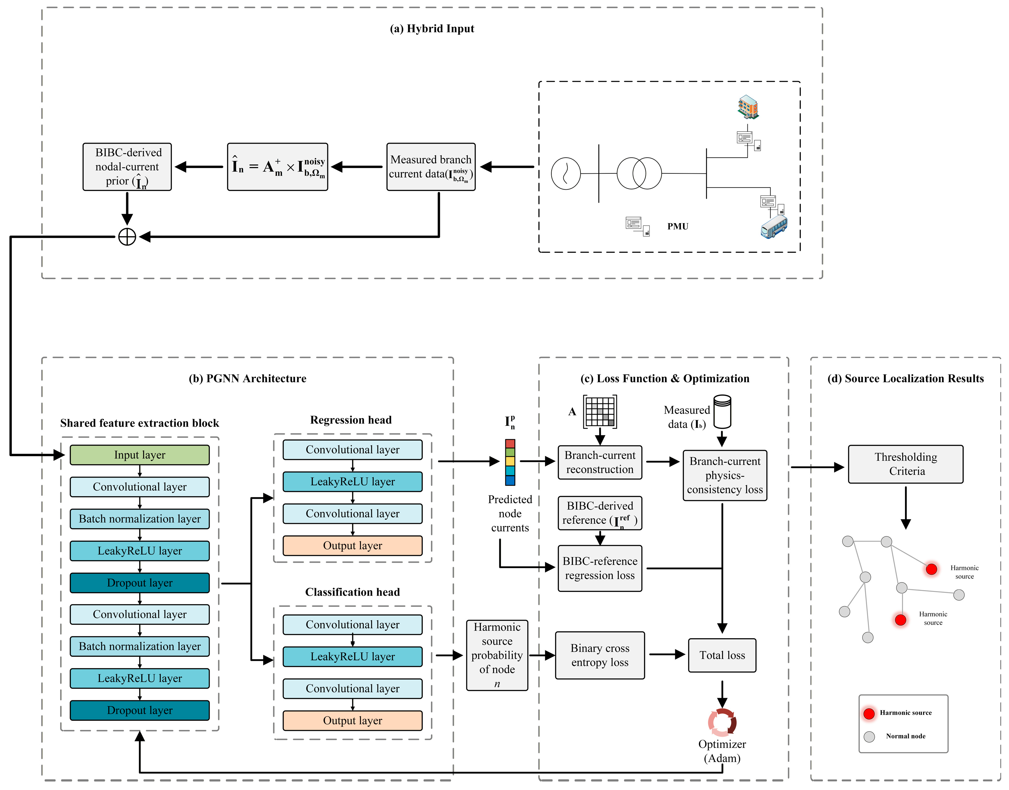
The proposed PGNN incorporates BIBC-based physical information into both the hybrid input and the training objective. The BIBC-derived nodal-current prior provides a topology-informed input representation, while the branch-current physics-consistency loss constrains the predicted nodal currents to reproduce the available branch-current phasors through the BIBC mapping. This design aims to improve prediction consistency under the measurement-noise, reduced-training-set, and reduced-PMU conditions evaluated in this study. Figure 1 illustrates the overall framework.

Figure 1. Framework of the proposed PGNN-based harmonic source localization and nodal harmonic injection-current estimation method.

The proposed framework consists of four main stages:

• Hybrid input construction;
• Shared CNN-based feature extraction and dual-head prediction;
• Physics-guided joint-loss optimization;
• Threshold-based source localization and conversion of the predicted nodal currents into magnitudes and phase angles.

In the first stage, the available branch harmonic-current phasors are combined with a BIBC-derived nodal-current prior to form the hybrid input vector. The prior is calculated from the available noisy branch-current measurements. In the second stage, a shared feature extractor and dual-head architecture jointly perform harmonic source localization and nodal harmonic injection-current estimation. The shared CNN module extracts latent features from the physics–data-fused input. Supervised by binary source-bus labels, the classification head outputs the probability that each bus is a harmonic source, whereas the regression head estimates the real and imaginary components of the nodal harmonic injection currents. In the third stage, the two heads are jointly optimized using three terms: a binary cross-entropy classification loss, a regression loss relative to the BIBC-derived reference, and a branch-current physics-consistency loss. The regression reference is calculated from complete noise-free simulated branch-current phasors and is not included in the network input. Finally, buses with predicted source probabilities greater than or equal to 0.5 are identified as harmonic sources, and the predicted real and imaginary current components are converted into magnitudes and phase angles.

In the lumped steady-state radial-network model adopted here, a discrete BIBC mapping derived from Kirchhoff’s current law relates branch currents to nodal injection currents. For radial distribution networks, the branch harmonic-current vector I_b and the nodal harmonic injection-current vector I_n are related by the following linear mapping:

I_b = AI_n

(6)

where A denotes the BIBC matrix of the distribution system.

Because PMUs are installed at only a subset of buses, harmonic-current phasors are available only for the corresponding observable branches. Let Ω_m denote the observable branch set and A_m the corresponding row submatrix of the BIBC matrix A. The Moore–Penrose pseudoinverse of A_m is denoted by ${\mathbf{A}}_m^{+}$. The BIBC-derived prior estimate of the nodal harmonic injection currents is then given by

$${\hat{\mathrm{I}}}_{\mathrm{n}}{=\mathrm{A}}_{\mathrm{m}}^{+}{\mathrm{I}}_{{\mathrm{b},\mathsf{\Omega }}_{\mathrm{m}}}^{\mathrm{noisy}}$$

(7)

where ${\widehat{\mathbf{I}}}_{\mathrm{n}}$ denotes the BIBC-derived nodal-current input prior and ${\mathbf{I}}_{\mathrm{b},{\mathsf{\Omega }}_{\mathrm{m}}}^{\mathrm{noisy}}$ denotes the available noisy branch-current measurements. Although this minimum-norm least-squares estimate may be affected by measurement sparsity and noise, it provides a topology-informed input feature that helps constrain the candidate solution space.

A hybrid input tensor X_h is constructed to integrate physical information with data-driven features. Branch-current entries that are unavailable under the current PMU configuration are first set to zero, yielding a masked branch-current tensor ${\tilde{\mathbf{I}}}_{\mathrm{b}}$. The pseudoinverse of the observable BIBC submatrix is then applied to the available branch currents to obtain the BIBC-derived nodal-current prior, denoted by ${\widehat{\mathbf{I}}}_{\mathrm{n}}$. Finally, the real and imaginary components of ${\tilde{\mathbf{I}}}_{\mathrm{b}}$ and ${\widehat{\mathbf{I}}}_{\mathrm{n}}$ are concatenated along the channel dimension to form the hybrid input tensor. The four channels correspond, respectively, to the real and imaginary components of the masked branch currents and the BIBC-derived nodal-current prior.

$${\mathrm{X}}_{\mathrm{h}}=[{\tilde{\mathrm{I}}}_{\mathrm{b}}^{\mathrm{Re}},{\tilde{\mathrm{I}}}_{\mathrm{b}}^{\mathrm{Im}}{,\hat{\mathrm{I}}}_{\mathrm{n}}^{\mathrm{Re}}{,\hat{\mathrm{I}}}_{\mathrm{n}}^{\mathrm{Im}}]\in {ℝ}^{N\times 4}$$

(8)

To distinguish the regression reference from the input prior, the complete noise-free simulated branch-current vector is transformed using the full BIBC pseudoinverse as ${\mathbf{I}}_{\mathrm{n}}^{\mathrm{ref}}={\mathbf{A}}^{+}{\mathbf{I}}_{\mathrm{b}}^{\mathrm{full},\mathrm{clean}}$. This BIBC-derived quantity is used only as the regression target during training and as the reference during evaluation; it is not included in the network input. Under complete branch-current observability, the BIBC matrix of the radial test system is square and nonsingular. Writing ${\mathbf{I}}_{\mathrm{b}}^{\mathrm{noisy}}={\mathbf{I}}_{\mathrm{b}}^{\mathrm{full},\mathrm{clean}}+\mathsf{\eta }$ gives ${\widehat{\mathbf{I}}}_{\mathrm{n}}={\mathbf{I}}_{\mathrm{n}}^{\mathrm{ref}}+{\mathbf{A}}^{-1}\mathsf{\eta }$. Thus, the input prior is a deterministic, topology-informed transformation of the noisy measurements and provides no additional independent measurement under complete observability.

In the radial test systems considered here, each non-substation bus is uniquely associated with its upstream branch. The masked branch-current vector and the nodal-current vector therefore have the same length N and are ordered according to the corresponding downstream buses. Let n denote the total number of buses, including the substation, and let N = n − 1 denote the number of non-substation buses and their corresponding upstream branches. The hybrid input allows the network to use available branch-current information together with an explicit topology-informed estimate of the nodal harmonic injection currents.

2.4. Design of the Loss Function

The overall objective jointly optimizes source localization and nodal harmonic injection-current estimation through three terms: a branch-current physics-consistency loss L_phy, a supervised classification loss L_sup, and a regression loss L_ref relative to the BIBC-derived reference. The BIBC matrix maps the predicted nodal harmonic injection currents ${\mathbf{I}}_{\mathrm{n}}^{\mathrm{p}}$ to branch currents. The mean squared error between reconstructed and available branch currents is calculated over the observable branch set Ω_m, where M = |Ω_m|. This term encourages the predicted nodal currents to be consistent with the BIBC mapping and the available measurements:

$$L_{\mathit{phy}}={\displaystyle \frac{1}{M}}{‖{\mathrm{A}}_{\mathrm{m}}{\mathrm{I}}_{\mathrm{n}}^{\mathrm{p}}{-\mathrm{I}}_{{\mathrm{b},\mathsf{\Omega }}_{\mathrm{m}}}^{\mathit{noisy}}‖}_2^2$$

(9)

The binary cross-entropy (BCE) loss optimizes the classification head by driving the predicted source-probability vector ${\widehat{\mathrm{p}}}_{\mathrm{s}}$ toward the binary source-bus label vector y_s:

$$L_{\sup }=\mathrm{BCE}({\stackrel{\mathrm{\Lambda }}{\mathrm{p}}}_{\mathrm{s}},\hspace{0.33em}{\mathrm{y}}_{\mathrm{s}})$$

(10)

Because independently measured nodal harmonic injection-current labels are unavailable, the BIBC-derived reference ${\mathbf{I}}_{\mathrm{n}}^{\mathrm{ref}}$, obtained from complete noise-free simulated branch-current phasors, is used as a simulation-derived pseudo-label for the regression head. The corresponding regression loss is defined as

$$L_{\mathrm{ref}}={\displaystyle \frac{1}{N}}\left[{‖\mathrm{Re}\left(I_n^p\right)-\mathrm{Re}\left(I_n^{\mathrm{ref}}\right)‖}_2^2+{‖\mathrm{Im}\left(I_n^p\right)-\mathrm{Im}\left(I_n^{\mathrm{ref}}\right)‖}_2^2\right]$$

(11)

Unlike the input prior ${\widehat{\mathbf{I}}}_{\mathrm{n}}$, which is calculated from the available noisy measurements and fed to the network, ${\mathbf{I}}_{\mathrm{n}}^{\mathrm{ref}}$ is calculated from the complete noise-free simulated branch currents and is used only for regression supervision and evaluation. It is therefore regarded as a BIBC-derived model reference rather than an independently measured ground truth.

Consequently, small regression errors indicate agreement with the adopted BIBC-derived reference; they do not independently establish the accuracy of the estimated nodal currents in a physical network.

Finally, the overall PGNN objective is formulated as a weighted linear combination of the three loss components:

L_total = λ_phyL_phy + λ_supL_sup + λ_refL_ref

(12)

where L_total denotes the overall loss and λ_phy, λ_sup and λ_ref are the weights of the branch-current physics-consistency loss, supervised classification loss, and regression loss relative to the BIBC-derived reference, respectively.

2.5. Parameter Settings of the PGNN Model

The proposed PGNN uses a fully convolutional one-dimensional architecture. The four-channel hybrid input is first processed by two shared Conv1D layers, each with 64 output channels, a kernel size of 3, a stride of 1, and a padding of 1. Each convolutional layer is followed by batch normalization, LeakyReLU activation with a negative slope of 0.2, and dropout at a rate of 0.2. No pooling or fully connected layers are used, so the spatial dimension N, corresponding to the number of non-substation buses, is preserved throughout the network. The regression head consists of two Conv1D layers with channel dimensions 64→32→2 and a kernel size of 3, producing the real and imaginary components of the nodal harmonic injection currents at all N buses. The classification head uses Conv1D layers with channel dimensions 64→32→1 and kernel sizes of 3 and 1, respectively, followed by a sigmoid function that produces one source probability per bus. Because the model is fully convolutional, its trainable parameter count depends on the channel dimensions rather than on N, resulting in approximately 0.026 M parameters for both test systems. The first convolution in each prediction head is followed by LeakyReLU activation with a negative slope of 0.2. Table A1 summarizes the layer-wise configuration and tensor shapes. The network contains 26,019 trainable parameters.

The model was trained for 400 epochs using Adam with a batch size of 128. The initial learning rate was 0.0032 and was multiplied by 0.2 every 125 epochs. The checkpoint with the lowest total validation loss was used for evaluation. The classification threshold was fixed at 0.5, and all three loss weights were set to 0.1.

3. Results and Discussion

The modified IEEE 13-bus and modified IEEE 33-bus distribution systems were used to evaluate the effectiveness and applicability of the proposed method [32]. All experiments were conducted on a desktop workstation equipped with a 10th-generation Intel Core i7-10750H processor and an NVIDIA GeForce GTX 1650 Ti GPU. MATLAB/Simulink (R2024b, Mathworks, Natick, MA, USA, 1984–2026) was used to generate the simulation data. Data preprocessing, cross-validation, model training, and performance evaluation were implemented in Python 3.11.7 using PyTorch 2.13.

3.1. Test System and PMU Placement

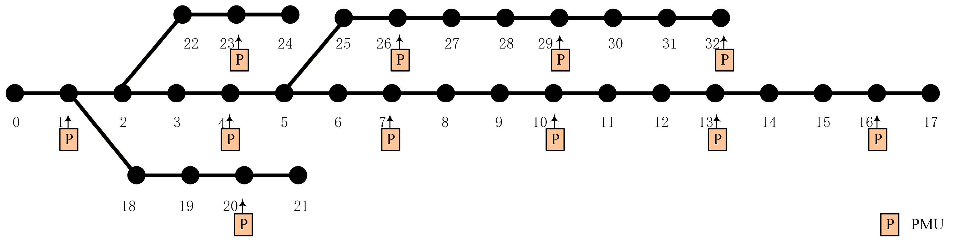
The proposed method was evaluated on the modified IEEE 13-bus and modified IEEE 33-bus distribution systems, both of which have a base voltage of 12.66 kV. The modified IEEE 13-bus system adopted in this study is a balanced three-phase system. The 12.66 kV base voltage was adopted to maintain consistency with the modified IEEE 33-bus system used in the simulations. In both systems, bus 0 denotes the substation, and each of the remaining buses is connected to a distribution transformer. The substation is represented by an ideal voltage source, and no finite source impedance is included in the present simulation model. In both the modified IEEE 13-bus and modified IEEE 33-bus systems, the transformer windings are connected in grounded wye on both sides (Yg–Yg). Thus, neither model includes a delta-connected winding that would provide the zero-sequence trapping mechanism associated with a Dyn connection. The PMU placement schemes are illustrated in Figure 2 and Figure 3. The observability criteria were defined as follows:

•

A bus is directly observable if a measurement device is installed at that bus;

•

If a bus voltage is observable, an adjacent bus is indirectly observable when the current in the connecting branch is measured;

•

A branch current is considered observable if the voltages at both terminal buses are observable.

To ensure complete state observability, PMUs were deployed at buses 1, 3, 5, 8, 9, and 10 in the modified IEEE 13-bus system and at buses 1, 4, 7, 10, 13, 16, 20, 23, 26, 29, and 32 in the modified IEEE 33-bus system. Only branch-current phasors identified as observable by the observability analysis were used as neural-network measurement inputs. Under the adopted PMU placement and observability rules, all branch currents were observable in the complete-observability experiments. In the numerical implementation, complete clean branch-current phasors were first generated in MATLAB/Simulink. The observability analysis then determined measurement availability: observable entries were retained as available inputs, whereas unavailable entries were masked.

Figure 2. Modified IEEE 13-bus distribution system with PMU placement.

Figure 2. Modified IEEE 13-bus distribution system with PMU placement.

Figure 3. Modified IEEE 33-bus distribution system with PMU placement.

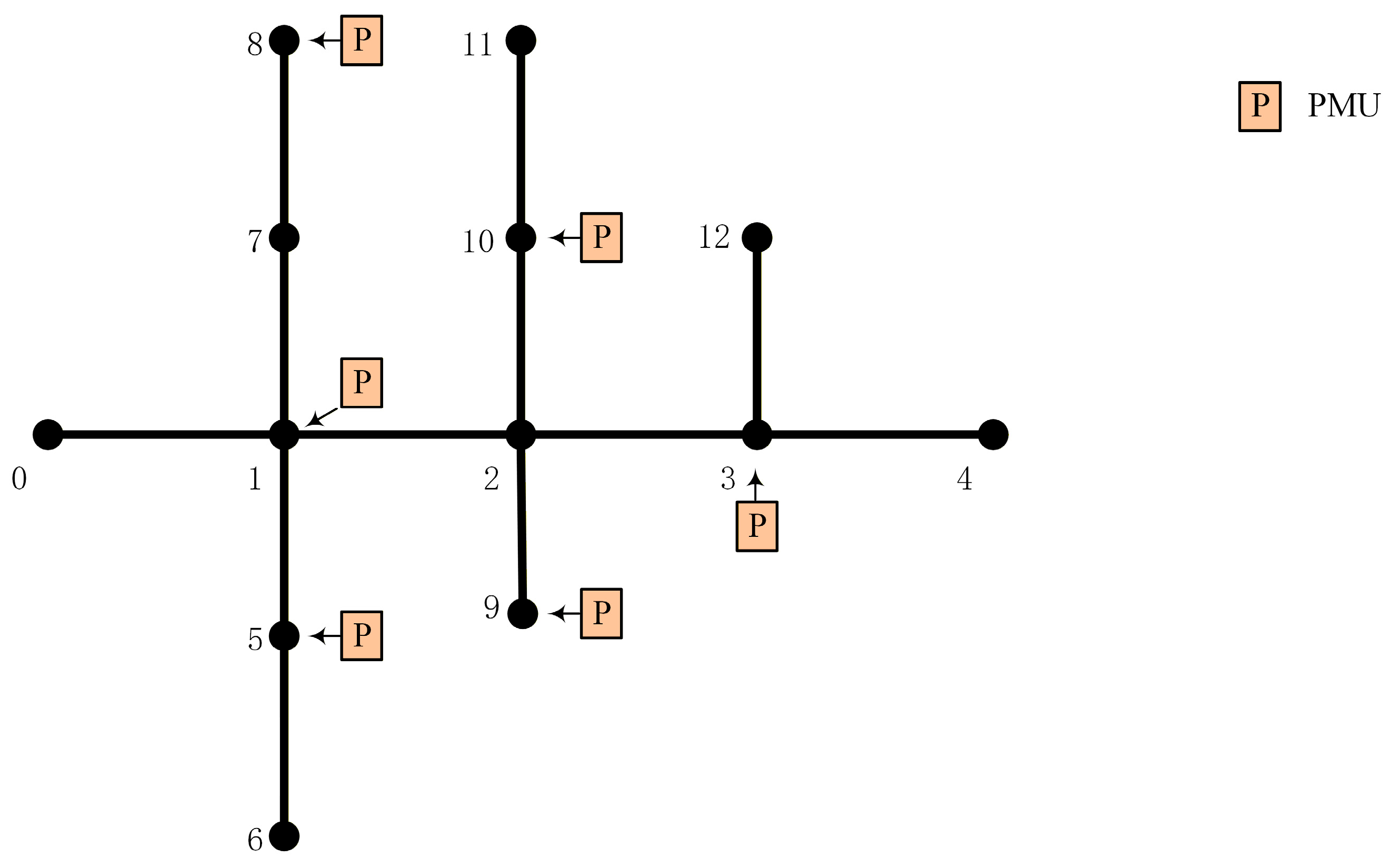
Figure 3. Modified IEEE 33-bus distribution system with PMU placement.

3.2. Simulation Scenarios and Evaluation Protocol

Several simulation scenarios were designed to represent a range of operating conditions and account for uncertainties in practical distribution-system operation, as summarized in Table 2.

Table 2. Simulation scenario settings.

Parameter	Value
Harmonic source-current magnitude (A)	(0, 2]
Phase angle	[−180°, 180°]
Harmonic orders	{3, 5, 7, 11}
Number of harmonic sources	1–5
Load and power generation scaling	80–120% of nominal value
Line parameter variation	{80%, 90%, 110%, 120%} of original value

For each sample, a common load and generation scaling factor was drawn uniformly from [0.8, 1.2], and all line parameters were multiplied by a factor randomly selected from {0.8, 0.9, 1.1, 1.2}. The number of harmonic sources was drawn uniformly from the integers 1–5, and the source buses were sampled without replacement from the non-substation buses. Accordingly, sample-wise cross-validation evaluated generalization to unseen operating samples without requiring disjoint source-bus combinations across folds. Source magnitudes and phase angles were drawn independently for each sample from the ranges in Table 2, while load and generation scaling factors and line-parameter variation factors were sampled according to the simulation settings. Samples sharing the same source-bus combination can have different harmonic source magnitudes and phase angles, resulting in different branch-current inputs.

The line-parameter variation in Table 2 is included only as part of the simulation-data-generation settings because the adopted BIBC matrix is topology-based and does not directly depend on line impedance or admittance parameters. For regression supervision and evaluation, a BIBC-derived nodal-current reference was constructed for each simulated sample. Before measurement noise was added, the complete noise-free simulated branch-current phasors were transformed using the full BIBC pseudoinverse to obtain ${\mathbf{I}}_{\mathrm{n}}^{\mathrm{ref}}$. This quantity served as a simulation-derived pseudo-label and evaluation reference rather than as an independently measured nodal-current ground truth. In contrast, the input prior ${\widehat{\mathbf{I}}}_{\mathrm{n}}$ was calculated only from the available noisy branch-current measurements.

The operating scenarios described above were simulated in MATLAB/Simulink to construct the harmonic source localization dataset. To enhance simulation fidelity, harmonic sources were randomly assigned to different buses, excluding substation bus 0, in both the modified IEEE 13-bus and modified IEEE 33-bus distribution systems to inject harmonic currents into the network. The dataset included four representative harmonic orders: the 3rd, 5th, 7th, and 11th harmonics. For the modified IEEE 13-bus system, 1000 samples were generated for each harmonic order, yielding 4000 samples in total. For the modified IEEE 33-bus system, 7000 samples were generated for each harmonic order, yielding 28,000 samples in total. Separate models were trained and evaluated for each system and for the 3rd, 5th, 7th, and 11th harmonic orders. The datasets were randomly partitioned into training, validation, and test sets, and five-fold cross-validation was used to mitigate the influence of random partitioning. The main comparisons used sample-wise five-fold cross-validation, with 70%, 10%, and 20% of the data allocated to training, validation, and testing in each fold. The additional PGNN-1 experiment used mutually exclusive source-combination groups with approximately the same proportions. Unless otherwise stated, reported metrics are unweighted means of the five test-fold values. Within each fold, two scalar sample standard deviations were calculated using only the clean training subset by pooling the real and imaginary branch-current components separately across samples and branches. These fixed training-derived scales were used to generate independent zero-mean Gaussian perturbations for the training, validation, and test inputs at nominal noise level α.

For a consistent multi-task comparison, CNN, FCNN, and GCN were also equipped with source-bus classification and nodal-current regression heads with the same output dimensions as those of PGNN. All four models used the same binary source-bus labels and the same BIBC-derived regression reference. The baseline models used the noisy branch-current phasors as their inputs and were optimized using classification and regression losses, whereas PGNN additionally used the BIBC-derived input prior and the branch-current physics-consistency loss. A classification threshold of 0.5 was used for all models. Detailed architectural configurations of the CNN, FCNN, and GCN baselines are provided in Table A2.

The models were evaluated using exact-match accuracy (EM), micro-averaged precision (Pr), micro-averaged recall (Re), micro-averaged F1-score [33], current-magnitude percentage error (PE₁), and mean circular absolute phase-angle error (E_θ).

$$\begin{array}{l}{\stackrel{\mathrm{\Lambda }}{\mathrm{y}}}_s=\mathbb{I}({\widehat{\mathrm{p}}}_s\ge 0.5)\\ \mathrm{EM}={\displaystyle \frac{1}{S}}{\displaystyle \sum _{s=1}^S\mathbb{I}}\left({\stackrel{\mathrm{\Lambda }}{\mathrm{y}}}_s{=\mathrm{y}}_s\right)\times 100\%\end{array}$$

(13)

$$\mathrm{Precision}={\displaystyle \frac{\mathrm{TP}}{\mathrm{TP}+\mathrm{FP}}}$$

(14)

$$\mathrm{Recall}={\displaystyle \frac{\mathrm{TP}}{\mathrm{TP}+\mathrm{FN}}}$$

(15)

$$\mathrm{F}1-\mathrm{score}=2\times {\displaystyle \frac{\mathrm{Precision}\times \mathrm{Recall}}{\mathrm{Precision}+\mathrm{Recall}}}$$

(16)

$$P{E}_1={\displaystyle \frac{100}{L}}{\displaystyle \sum _{s=1}^S{\displaystyle \sum _{i\in S_s}\frac{\left|\left|{\mathrm{I}}_{\mathrm{s},\mathrm{i}}^{\mathrm{p}}\right|-\left|{\mathrm{I}}_{\mathrm{s},\mathrm{i}}^{\mathrm{ref}}\right|\right|}{\left|{\mathrm{I}}_{\mathrm{s},\mathrm{i}}^{\mathrm{ref}}\right|+\epsilon }}}$$

(17)

$$\begin{array}{l}{E}_{\theta }={\displaystyle \frac{1}{L}}{\displaystyle \sum _{s=1}^S{\displaystyle \sum _{i\in S_s}\min \left(d_{s,i},{360}^{\circ }-d_{s,i}\right)}}\\ d_{s,i}=\mathrm{mod}\left(\left|\angle {\mathrm{I}}_{\mathrm{s},\mathrm{i}}^{\mathrm{p}}-\angle {\mathrm{I}}_{\mathrm{s},\mathrm{i}}^{\mathrm{ref}}\right|,{360}^{\circ }\right)\end{array}$$

(18)

where S is the number of test samples; ${\widehat{\mathrm{y}}}_{\mathrm{s}}$ is the corresponding binary source-label vector obtained using the fixed threshold of 0.5; TP, FP, TN, and FN denote the numbers of true-positive, false-positive, true-negative, and false-negative bus-level decisions, respectively; S_s is the set of ground-truth harmonic source buses in sample s; ε is a small positive constant used to avoid division by zero; and L is the total number of ground-truth source buses in the test set. For Pr, Re, and F1-score, TP, FP, and FN are pooled across all sample–bus decisions within each test fold. Both PE₁ and E_θ are averaged only over ground-truth source buses, regardless of whether those buses are correctly classified. In Equations (17) and (18), the current-magnitude and phase-angle differences are evaluated against the BIBC-derived reference. Thus, PE₁ and E_θ quantify reference-relative reconstruction errors. The term ground-truth source buses refers to the source-location labels of the simulated scenarios, not to independently measured nodal-current phasors. For PE₁ and E_θ, the raw regression-head outputs are used at all ground-truth source buses, regardless of the classification decision. A missed source bus is therefore not assigned zero current; its raw regression output is retained in the error calculation. Here, ε = 10⁻⁸ is used only to avoid numerical division by zero.

3.3. Harmonic Source Localization Under Complete System Observability

3.3.1. Analysis of Harmonic Source Localization Results

Experiments were performed on the modified IEEE 13-bus and modified IEEE 33-bus distribution systems to evaluate the proposed method for harmonic source localization. The 3rd, 5th, 7th, and 11th harmonic orders were considered, with 5% Gaussian noise added to the measurement data. The real and imaginary noise standard deviations were set to 0.05σ_Re and 0.05σ_Im, respectively, using the training-set statistics defined in Section 3.2. To evaluate PGNN generalization under a more challenging data-partitioning scheme, an additional experiment, denoted PGNN-1, was conducted on the modified IEEE 13-bus system using source-combination-disjoint five-fold cross-validation. PGNN-1 used the same network architecture and training hyperparameters as the original PGNN, differing only in its source-combination-disjoint cross-validation scheme. The training, validation, and test subsets contain mutually exclusive source-bus combinations, while the individual source buses remain represented in the training data. Table 3 summarizes EM and F1-score for both systems, including PGNN-1 on the 13-bus system. Table A3 provides the complete classification results, including precision and recall.

Table 3. Performance c omparison of h armonic s ource l ocalization.

System	Model	3rd		5th		7th		11th
		EM (%)	F1 (%)	EM (%)	F1 (%)	EM (%)	F1 (%)	EM (%)	F1 (%)
IEEE13	PGNN	99.80	99.95	100.0	100.0	100.0	100.0	100.0	100.0
	PGNN-1	99.70	99.92	99.90	99.97	99.70	99.92	98.12	99.52
	CNN	98.10	99.50	98.10	99.52	97.00	99.22	98.50	99.60
	FCNN	95.60	98.88	96.70	99.17	96.70	99.16	97.00	99.24
	GCN	98.30	99.54	99.00	99.75	98.10	99.52	97.50	99.32
IEEE33	PGNN	99.96	99.99	99.78	99.95	99.97	99.99	99.90	99.97
	CNN	97.39	99.49	98.16	99.45	98.61	99.62	97.98	99.43
	FCNN	95.42	99.06	95.62	98.89	95.82	98.94	93.21	98.27
	GCN	98.99	99.79	98.41	99.56	98.41	99.57	96.79	99.17

As shown in Table 3, under the original sample-wise five-fold cross-validation protocol, PGNN achieves the highest EM and F1-score among the four models for every tested harmonic order on both systems. On the modified IEEE 33-bus system, its EM ranges from 99.78% to 99.97%, whereas the EM values of the baselines range from 93.21% to 98.99%. These sample-wise results compare model performance on unseen operating samples without requiring source-bus combinations to be disjoint across the training, validation, and test subsets. Under the tested 5% Gaussian-noise condition, the observed improvement should be attributed to the overall PGNN framework rather than any single component, because PGNN differs from the baselines in both its BIBC-informed input representation and its training objective. Separately, PGNN-1 achieves EM values of 98.12–99.90% under source-combination-disjoint five-fold cross-validation on the modified IEEE 13-bus system. This group-disjoint evaluation assesses generalization to unseen source-bus combinations, while the individual source buses remain represented in the training data. The PGNN-1 results therefore provide supplementary evidence of PGNN generalization within this simulated setting, rather than a direct performance comparison with the baselines evaluated under the sample-wise protocol.

3.3.2. Estimation of Harmonic Source Injection Currents

Experiments were conducted on the modified IEEE 13-bus and modified IEEE 33-bus distribution systems to evaluate nodal harmonic injection-current reconstruction relative to the BIBC-derived reference. For the four harmonic orders considered (the 3rd, 5th, 7th, and 11th harmonics), 5% Gaussian noise was added to the measurement data. Table 4 compares the regression performance of PGNN, CNN, FCNN, and GCN in terms of PE₁ and mean circular absolute phase-angle error. It also reports the PGNN-1 results for the modified IEEE 13-bus system.

Table 4. Nodal harmonic injection-current estimation errors relative to the BIBC-derived reference.

System	Model	Mean Test Samples per Fold	3rd		5th		7th		11th
			PE1 (%)	Eθ (°)	PE1 (%)	Eθ (°)	PE1 (%)	Eθ (°)	PE1 (%)	Eθ (°)
IEEE13	PGNN	200	5.53	1.96	5.74	1.94	6.21	2.03	4.66	1.64
	PGNN-1	200	5.80	1.85	5.90	1.87	6.27	1.93	7.03	2.12
	CNN	200	13.32	6.75	11.84	5.89	12.75	5.96	13.87	5.39
	FCNN	200	9.04	2.65	8.00	2.63	8.33	2.63	8.96	3.55
	GCN	200	13.16	5.43	11.64	5.14	12.39	5.28	13.91	6.16
IEEE33	PGNN	1400	4.24	1.85	5.75	1.95	5.65	1.93	7.22	2.11
	CNN	1400	16.02	7.39	42.77	34.94	41.83	33.90	34.85	26.05
	FCNN	1400	8.36	3.15	11.86	3.94	12.86	4.44	12.61	4.61
	GCN	1400	13.63	7.46	39.20	31.63	40.77	32.59	34.67	25.19

Note: All PE₁ values are evaluated relative to the BIBC-derived nodal-current reference.

Table 4 shows that, under the original sample-wise split, PGNN yields the lowest current-magnitude and phase-angle errors relative to the BIBC-derived reference among the four models for every tested system and harmonic-order combination. PGNN-1 yields similar regression errors at the 3rd, 5th, and 7th harmonics, while PE₁ increases from 4.66% to 7.03% at the 11th harmonic. On the modified IEEE 33-bus system, PGNN yields PE₁ values ranging from 4.24% to 7.22%. PGNN achieves lower reference-relative regression errors than the three learning-based baselines under the nominal 5% noise condition. In the original sample-wise comparison, all four models were trained using the same regression reference, whereas PGNN additionally used the BIBC-derived input prior and the branch-current physics-consistency loss. These results compare the full model configurations and do not isolate the effects of the input prior and consistency loss. The comparison is specific to this model-derived reference and does not, by itself, validate the estimates against independently obtained nodal-current phasors.

3.3.3. Computational Efficiency and Complexity Analysis of Different Models

The third harmonic under 5% Gaussian noise was used as a representative case to compare localization performance and computational cost across the two test-system sizes. CNN, FCNN, and GCN served as baselines. All models were evaluated using the same cross-validation folds, noise realizations, epoch budget, batch size, classification threshold, hardware platform, and random seed. Performance was assessed in terms of trainable parameter count, FLOPs, training-set EM, test-set EM, training time, and test-fold evaluation time. The reported evaluation time is the mean wall-clock time for batched processing of one complete test fold. It includes hybrid-input assembly using a precomputed pseudoinverse and does not measure single-frame or end-to-end PMU latency. Table 5 summarizes the results.

Table 5. Performance and computational efficiency comparison of four models.

System	Model	Params (M)	FLOPs (M)	Train-Set EM (%)	Test-Set EM (%)	Train Time (s)	Test-Fold Evaluation Time (s)
IEEE13	PGNN	0.026	0.66	100.0	99.80	21.08	0.0095
	CNN	0.349	3.41	100.0	98.10	26.35	0.0098
	FCNN	1.135	2.26	100.0	95.60	22.35	0.0086
	GCN	0.472	2.14	100.0	98.30	30.08	0.0106
IEEE33	PGNN	0.026	1.69	100.0	99.96	168.08	0.0635
	CNN	0.681	9.00	98.94	97.39	191.57	0.0620
	FCNN	1.159	2.31	99.04	95.42	162.41	0.0591
	GCN	1.133	5.98	99.65	98.99	205.19	0.0684

As shown in Table 5, PGNN provides a favorable trade-off between localization accuracy and computational complexity on the two tested systems. It achieves test-set EM values of 99.80% and 99.96% on the modified IEEE 13-bus and modified IEEE 33-bus systems, respectively, outperforming CNN, FCNN, and GCN. PGNN uses only 0.026 M trainable parameters for both systems, while its FLOPs increase from 0.66 M to 1.69 M as the system size increases. On the modified IEEE 33-bus system, both its parameter count and FLOPs are lower than those of the three baselines.

The test-fold evaluation time of PGNN is comparable to the evaluation times of the baseline models. Although FCNN is slightly faster, PGNN achieves higher test-set EM with substantially fewer parameters. CNN and FCNN do not explicitly incorporate BIBC-based constraints, while the tested GCN performs graph-based feature propagation without directly using the feeder BIBC matrix. In contrast, PGNN incorporates BIBC-derived information through both the hybrid input and the physics-consistency loss, resulting in a favorable accuracy–complexity trade-off across the two tested systems.

3.3.4. Performance Under Different Measurement-Noise Levels

To evaluate model performance under additive measurement noise, zero-mean Gaussian noise was added to the real and imaginary components of the third-harmonic branch-current phasors from the modified IEEE 33-bus system. The noise standard deviations were ασ_Re and ασ_Im for the real and imaginary components, respectively, using the training-set statistics defined in Section 3.2, with α∈{0,0.05,0.10,0.15,0.20}. The dataset-level RMS TVE-equivalent is defined in Equation (A1), and the calibrated values are reported in Table A4. These values characterize the simulated noise severity and do not constitute a PMU standards-compliance test. A separate model was trained and evaluated at each noise level using matched training, validation, and test noise conditions. The results therefore characterize performance under matched noise levels, rather than the response of a single fixed model to an unknown increase in noise. Data partitions were held fixed across noise levels.

A direct solution method based on the BIBC pseudoinverse, denoted Pinv, was also introduced. Pinv reconstructs nodal harmonic injection currents from branch-current measurements and identifies harmonic source buses by thresholding the estimated current magnitudes. The threshold was selected using only the validation subset of each fold and then fixed for testing.

As shown in Table 6, EM generally decreases and PE₁ generally increases with the noise level. Among the four learning-based models, PGNN consistently achieves the highest EM and the lowest PE₁. PGNN and Pinv achieve similar EM under low-noise conditions, but the EM advantage of PGNN becomes more pronounced as noise increases. At 20% noise, PGNN retains an EM of 82.99%, compared with 54.83% for Pinv.

Table 6. Performance evaluation under different nominal noise levels.

System	Model	Metric	Nominal Noise Level (%)
			0%	5%	10%	15%	20%
IEEE33	PGNN	EM (%)	100.0	99.96	97.58	91.79	82.99
	CNN		97.93	97.39	95.29	89.04	80.74
	FCNN		95.68	95.42	89.93	82.36	72.66
	GCN		99.03	98.99	95.20	90.49	82.17
	Pinv		100.0	99.86	94.74	76.53	54.83
	PGNN	PE1 (%)	4.82	4.24	7.47	9.70	12.19
	CNN		13.61	16.02	16.98	19.99	23.19
	FCNN		7.34	8.36	13.14	16.95	21.06
	GCN		11.07	13.63	16.50	18.58	22.59
	Pinv		6 × 10−9	3.09	6.17	9.23	12.26

Pinv yields lower reference-relative PE₁ values from 0% to 15% noise, whereas the two methods have nearly identical errors at 20% noise (12.19% for PGNN and 12.26% for Pinv). This result is consistent with Pinv directly reconstructing nodal currents through the same BIBC mapping used to construct the regression reference.

Overall, Pinv provides a strong non-learned reference under complete observability and low-noise conditions, while PGNN maintains substantially higher source-set localization accuracy as measurement noise increases. The present Gaussian-noise experiments do not establish robustness to non-Gaussian noise, synchronization errors, or bad data; these conditions require further evaluation.

3.3.5. Performance Under Reduced Training-Set Sizes

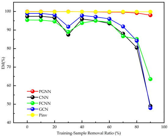
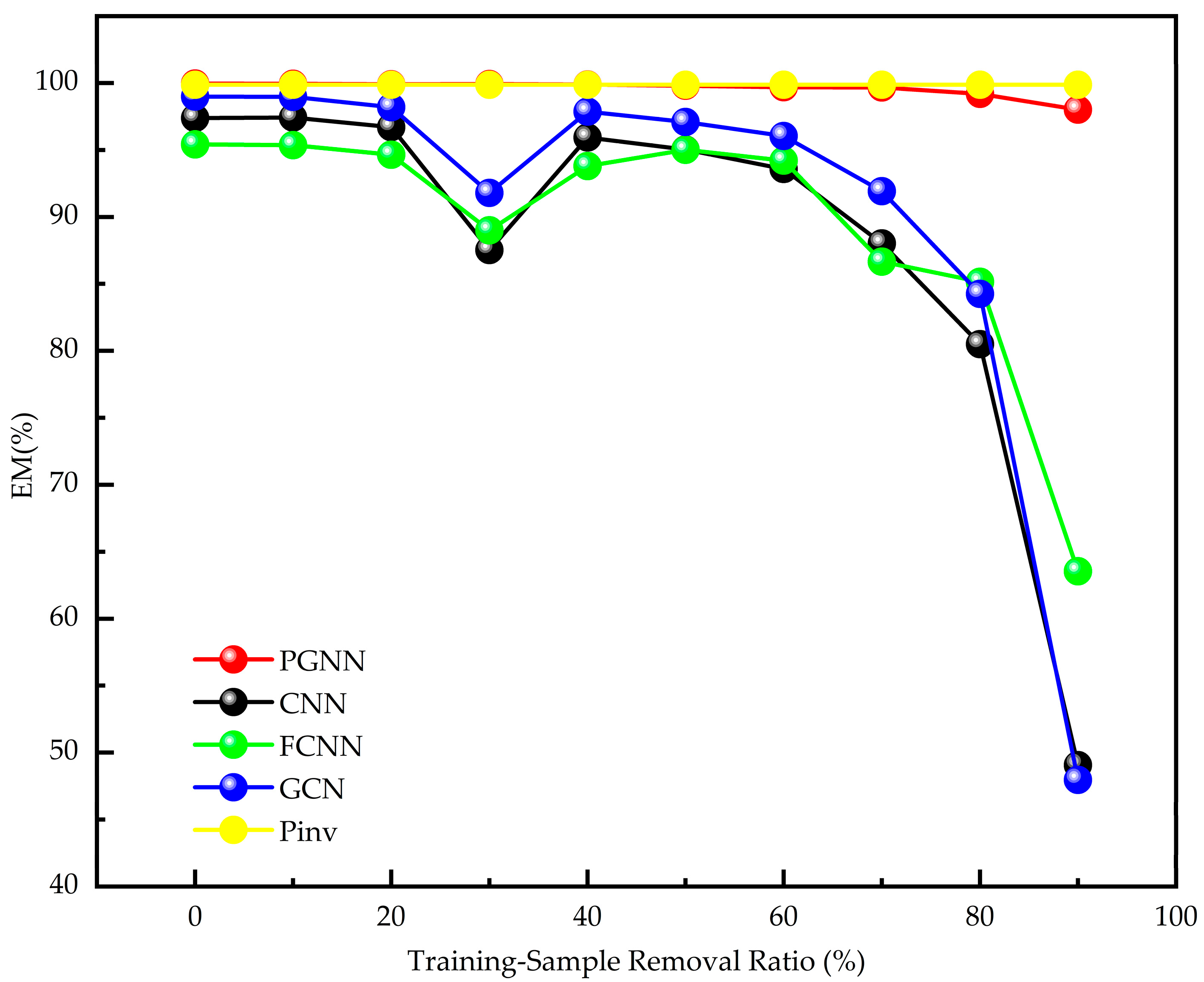
Additional experiments evaluated the proposed method with reduced training-set sizes by varying the training-sample removal ratio. Starting from the 7000 third-harmonic samples generated in Section 3.2, different proportions of samples were randomly removed from the training subset, with r∈{0%,10%,20%,30%,40%,50%,60%,70%,80%,90%}. PGNN was compared with CNN, FCNN, and GCN under these reduced-training-set scenarios, with Pinv included as a direct BIBC-based reference. Figure 4 compares their exact-match accuracy across the training-sample removal ratios.

Figure 4. Exact-match accuracy under varying training-sample removal ratios using a single random-removal seed (42), together with the Pinv reference. Results for the learning-based models are averaged over five test folds; Pinv remains unchanged because it does not depend on training-set size.

At each removal ratio, only the training subset of each cross-validation fold was randomly reduced; the validation and test subsets remained unchanged. The Gaussian-noise level was kept at 5%, and PGNN, CNN, FCNN, and GCN were retrained from scratch for each removal ratio. Because Pinv does not depend on model training or training-set size, its result at 5% noise remains unchanged across removal ratios and is shown as a horizontal reference. A single random-removal seed (42) was used in the reported experiment.

As shown in Figure 4, EM generally decreases as the training-sample removal ratio increases. In the tested random-removal trial, PGNN retains an EM above 99% for r ≤ 70% and achieves 99.19% and 98.01% at r = 80% and r = 90%, respectively. CNN, FCNN, and GCN exhibit greater performance degradation as the training data are reduced. In this single-seed experiment, PGNN shows a smaller decrease in EM than the three learning-based baselines as the training set is reduced. However, at the highest removal ratios, its EM falls below that of the Pinv reference.

Figure 4 reports the mean EM across five test folds using a single random-removal seed (42). Because variability across independent removal seeds was not evaluated, these results, including the 98.01% EM at 90% removal, should be interpreted as descriptive rather than as evidence of consistent robustness to training-sample removal.

3.3.6. Ablation Study and Loss-Weight Sensitivity Analysis

To distinguish the effects of the BIBC-derived input prior and the branch-current physics-consistency loss, a controlled 2 × 2 ablation was conducted on the modified IEEE 33-bus third-harmonic dataset under 5% Gaussian noise and complete branch-current observability. Four variants were evaluated: G00, without either component; G01, with the consistency loss only; G10, with the input prior only; and G11, with both components. All four variants used the same PGNN backbone. Removing the prior meant replacing its two input channels with zeros, while removing the consistency term meant setting its loss weight to zero. Thus, G00 is an ablation of the compact PGNN backbone, not the separate CNN baseline in Table 3.

As shown in Table 7, the BIBC-derived input prior accounts for the main improvement in source localization. Adding the prior increases EM from 49.46% to 99.86% without the physics-consistency loss and produces a similar improvement when that loss is retained. In contrast, the physics-consistency loss alone does not improve localization performance. When combined with the BIBC-derived prior, however, it reduces PE₁ from 5.26% to 4.24% and the phase-angle error from 2.50° to 1.85°. These results indicate that the prior is the main contributor to source localization, while the physics-consistency loss further improves current reconstruction relative to the BIBC-derived reference. Without the input prior, adding the consistency loss increases PE₁ from 20.74% to 24.13%. Its regression benefit is therefore conditional on the input representation in this experiment.

Table 7. Controlled ablation of the BIBC input prior and physics-consistency loss on the modified IEEE 33-bus system.

Variant	BIBC Prior	Physics Loss	EM (%)	F1 (%)	PE1 (%)	Eθ (°)
G00	No	No	49.46 ± 0.95	88.31 ± 0.13	20.74 ± 0.47	7.45 ± 0.23
G01	No	Yes	48.83 ± 0.96	88.10 ± 0.32	24.13 ± 0.48	7.37 ± 0.18
G10	Yes	No	99.86 ± 0.11	99.97 ± 0.02	5.26 ± 0.46	2.50 ± 0.08
G11	Yes	Yes	99.96 ± 0.04	99.99 ± 0.03	4.24 ± 0.52	1.85 ± 0.09

Note: Values are mean ± sample standard deviation across five test folds. Bold values indicate the best mean in each metric and do not imply statistical significance. Yes or No means whether this loss exists.

A loss-weight sensitivity experiment was conducted using the complete G11 configuration to further examine the interaction between the physics-consistency loss and the regression loss. Because L_phy constrains predictions using noisy branch-current measurements whereas L_ref is based on the clean BIBC-derived reference, their relative weights may affect regression performance. Therefore, λ_sup and λ_ref were fixed at 0.1, while λ_phy was set to 0.01, 0.1, and 1.0. These settings correspond to λ_phy/λ_ref ratios of 0.1, 1, and 10, respectively, spanning two orders of magnitude.

As shown in Table 8, overall performance remains stable across the tested weight range. EM ranges from 99.91% to 99.96%, while PE₁ ranges from 4.17% to 4.37%. The setting λ_phy = 0.1 yields the highest EM and the lowest phase-angle error, whereas λ_phy = 0.01 yields a slightly lower PE₁. These results indicate that PGNN is not highly sensitive to the relative weights of the two regression-related losses within the tested range, and the adopted value λ_phy = 0.1 provides a reasonable overall balance.

Table 8. Sensitivity of PGNN performance to the relative weighting of the physics-consistency and reference regression losses.

λphy	λref	Ratio	EM (%)	F1 (%)	PE1 (%)	Eθ (°)
0.01	0.1	0.1	99.94 ± 0.06	99.99 ± 0.01	4.17 ± 0.47	1.99 ± 0.06
0.1	0.1	1.0	99.96 ± 0.04	99.99 ± 0.03	4.24 ± 0.52	1.85 ± 0.09
1.0	0.1	10.0	99.91 ± 0.09	99.98 ± 0.02	4.37 ± 0.77	1.97 ± 0.10

3.4. Performance Under Reduced-PMU Configurations

The modified IEEE 33-bus system was used to evaluate model robustness to reduced measurement availability without retraining, using third-harmonic data with 5% Gaussian noise. All learning-based models were first trained under the complete 11-PMU measurement configuration. During testing, PMUs were progressively removed in the order 10, 29, 13, 7, 16, and 32. After each removal, bus and branch observability were recalculated according to the rules in Section 3.1. Measurements provided by the removed PMU were discarded, and branch-current entries that were no longer directly or indirectly observable under the remaining PMU configuration were masked.

In each cross-validation fold, PGNN, CNN, FCNN, and GCN were trained only once under complete measurement availability. Their parameters were then frozen, and the models were directly evaluated under different reduced-PMU configurations. Pinv was also included as a direct BIBC-based reference. Thus, the results in Table 9 represent zero-shot performance under measurement loss rather than performance obtained through configuration-specific retraining.

Table 9. Harmonic source localization under reduced-PMU configurations.

System	Number of PMUs	Removed PMU Locations	EM (%)
			PGNN	CNN	FCNN	GCN	Pinv
IEEE33	11	None	99.96	97.39	95.42	98.99	99.86
	10	10	98.67	96.46	94.36	98.20	96.19
	9	10, 29	96.81	95.64	92.40	96.37	81.23
	8	10, 13, 29	92.30	91.73	89.21	92.76	78.57
	7	7, 10, 13, 29	88.99	84.61	82.16	87.29	62.54
	6	7, 10, 13, 16, 29	85.86	78.74	77.93	81.59	60.44
	5	7, 10, 13, 16, 29, 32	78.89	75.19	72.64	77.11	58.27

As shown in Table 9, EM generally decreases for all methods as the number of available PMUs is reduced. The EM of PGNN decreases from 99.96% under the complete 11-PMU configuration to 78.89% with five PMUs remaining. PGNN achieves the highest EM in six of the seven tested configurations, while GCN achieves a slightly higher EM when eight PMUs remain (92.76% versus 92.30%). With five PMUs remaining, PGNN retains an EM of 78.89%, compared with 77.11% for GCN, 75.19% for CNN, 72.64% for FCNN, and 58.27% for Pinv.

In the configurations reported in Table 9, PGNN generally achieves higher EM than the other evaluated methods without retraining, whereas Pinv exhibits a larger decline in EM as measurement availability decreases. These results characterize source localization performance under the selected measurement-loss conditions, with the parameters of all learning-based models held fixed.

Table A5 in Appendix A reports an additional PMU-removal sequence, in which PMUs are removed in the order 7, 16, 10, 13, 32, and 26. With five PMUs remaining, PGNN achieves an EM of 50.229%, compared with 51.157% for GCN, 47.957% for CNN, and 45.571% for FCNN. The difference from the 78.89% EM obtained with five PMUs in Table 9 indicates sensitivity to the remaining PMU configuration rather than PMU count alone. PGNN therefore provides a localization advantage in several tested configurations, but this advantage is not uniform across all configurations. The reduced-PMU results should accordingly be interpreted as configuration-dependent performance under measurement loss.

4. Conclusions

This paper proposes a BIBC-guided PGNN for joint harmonic source localization and nodal harmonic injection-current estimation from limited PMU measurements. The model combines branch-current phasors with a BIBC-derived nodal-current prior. A shared feature extractor and two prediction heads are jointly optimized using source-bus supervision, BIBC-derived regression supervision, and a branch-current physics-consistency loss.

On the modified IEEE 13-bus and modified IEEE 33-bus systems, PGNN achieves the highest EM and F1-score among the compared learning-based models under complete branch-current observability and 5% Gaussian noise. It also yields lower current-magnitude and phase-angle errors relative to the BIBC-derived reference. On the modified IEEE 13-bus system under 5% Gaussian noise, source-combination-disjoint evaluation shows that PGNN retains high localization accuracy for source combinations unseen during training. The ablation study indicates that the BIBC-derived input prior accounts for the main improvement in source localization, while the physics-consistency loss further improves current reconstruction when combined with the prior.

In the matched-noise experiments on the modified IEEE 33-bus third-harmonic dataset, PGNN achieves an EM of 82.99% and a reference-relative PE₁ of 12.19% at a nominal Gaussian-noise level of 20%. A separate model is trained and evaluated at each noise level. Compared with Pinv, PGNN achieves higher source-set localization accuracy at the tested nonzero noise levels, whereas Pinv yields lower reference-relative PE₁ values from 0% to 15% noise. These results indicate different strengths in source localization and current reconstruction relative to the adopted reference.

In the reduced-PMU experiments, the learning-based models were trained under complete measurement availability and evaluated after PMU removal without retraining or fine-tuning. With five PMUs remaining, PGNN achieves EM values of 78.89% and 50.229% under the two tested PMU-removal sequences. These results show that localization performance depends on the remaining PMU configuration, not solely on the number of PMUs. PGNN achieves higher EM than the other learning-based models in several tested configurations, but its relative advantage is configuration-dependent.

The conclusions are limited to fixed radial topologies, simulated data, and the tested measurement-loss configurations. For known radial reconfigurations, the BIBC matrix, its observable submatrix, and the associated pseudoinverses should be updated, and topology-specific retraining and validation are recommended. Weakly meshed systems require an extension of the current formulation. In addition, the reported current errors are evaluated relative to the BIBC-derived reference rather than independent ground truth. Further validation using directly recorded simulated currents and field measurements is therefore required.

References

- Yang, R.; Peng, S.; Yao, G. A Multi-Modal Feature Combination Mechanism for Identification of Harmonic Load in Distribution Networks Based on Artificial Intelligence Models. Int. J. Electr. Power Energy Syst. 2025, 166, 110519. [Google Scholar] [CrossRef] [Scilit]
- Yin, S.; Sun, Y.; Xu, Q.; Sun, K.; Li, Y.; Ding, L.; Liu, Y. Multi-Harmonic Sources Identification and Evaluation Method Based on Cloud-Edge-End Collaboration. Int. J. Electr. Power Energy Syst. 2024, 156, 109681. [Google Scholar] [CrossRef] [Scilit]
- Nakhodchi, N.; Bollen, M.H.J.; Busatto, T. Transfer of Harmonics in Distribution Networks. IEEE Trans. Power Deliv. 2022, 37, 1617–1626. [Google Scholar] [CrossRef] [Scilit]
- Boroujeni, K.M.; Safargholi, F.; Malekian, K. A Harmonic Model Validation Methodology for Power Generation Units Based on Voltage-Current Phasor Characteristic. Int. J. Electr. Power Energy Syst. 2025, 165, 110494. [Google Scholar] [CrossRef] [Scilit]
- Hu, Z.; Han, Y.; Zalhaf, A.S.; Zhou, S.; Zhao, E.; Yang, P. Harmonic Sources Modeling and Characterization in Modern Power Systems: A Comprehensive Overview. Electr. Power Syst. Res. 2023, 218, 109234. [Google Scholar] [CrossRef] [Scilit]
- Safargholi, F.; Malekian, K.; Schufft, W. On the Dominant Harmonic Source Identification—Part I: Review of Methods. IEEE Trans. Power Deliv. 2018, 33, 1268–1277. [Google Scholar] [CrossRef] [Scilit]
- Safargholi, F.; Malekian, K.; Schufft, W. On the Dominant Harmonic Source Identification—Part II: Application and Interpretation of Methods. IEEE Trans. Power Deliv. 2018, 33, 1278–1287. [Google Scholar] [CrossRef] [Scilit]
- Xu, F.; Wang, C.; Guo, K.; Shu, Q.; Ma, Z.; Zheng, H. Harmonic Sources’ Location and Emission Estimation in Underdetermined Measurement System. IEEE Trans. Instrum. Meas. 2021, 70, 9003511. [Google Scholar] [CrossRef] [Scilit]
- Carta, D.; Muscas, C.; Pegoraro, P.A.; Solinas, A.V.; Sulis, S. Compressive Sensing-Based Harmonic Sources Identification in Smart Grids. IEEE Trans. Instrum. Meas. 2021, 70, 9000810. [Google Scholar] [CrossRef] [Scilit]
- Yang, R.; Tai, N.; Yu, M.; Huang, W.; Zhang, H.; Li, H. Multiple Harmonic Source Location Based on Orthogonal Matching Pursuit Algorithm. In Proceedings of the 11th International Conference on Renewable Power Generation: Meeting Net Zero Carbon (RPG 2022), London, UK, 22–23 September 2022; pp. 105–109. [Google Scholar]
- Zhou, W.; Wu, Y.; Huang, X.; Lu, R.; Zhang, H.-T. A Group Sparse Bayesian Learning Algorithm for Harmonic State Estimation in Power Systems. Appl. Energy 2022, 306, 118063. [Google Scholar] [CrossRef] [Scilit]
- Melo, I.D.; Pereira, J.L.R.; Ribeiro, P.F.; Variz, A.M.; Oliveira, B.C. Harmonic State Estimation for Distribution Systems Based on Optimization Models Considering Daily Load Profiles. Electr. Power Syst. Res. 2019, 170, 303–316. [Google Scholar] [CrossRef] [Scilit]
- Lin, Q.; Li, M.; Feng, S.; Yang, J.; Sun, X.; Li, J.; Wang, Z.; Xie, X. Harmonic Source Localization Based on the Joint Entropy Method. In Proceedings of the 2022 IEEE/IAS Industrial and Commercial Power System Asia (I&CPS Asia), Shanghai, China, 8–11 July 2022; pp. 282–286. [Google Scholar]
- Wu, W.; Zeng, D.; Li, J.; Lu, J.; Li, C.; Liu, S. Harmonic State Estimation and Localization Based on Broad-Band Measurement. Front. Energy Res. 2023, 11, 1320433. [Google Scholar] [CrossRef] [Scilit]
- Armenta, L.A.H.; Romero, D.R. Multiple Harmonic Source Location Using the Least Median of Squares Method with the Presence of Outliers in High Voltage Electric Power Systems. Electr. Power Compon. Syst. 2019, 47, 1375–1387. [Google Scholar] [CrossRef] [Scilit]
- Fernandes, R.A.S.; Oleskovicz, M.; da Silva, I.N. Harmonic Source Location and Identification in Radial Distribution Feeders: An Approach Based on Particle Swarm Optimization Algorithm. IEEE Trans. Ind. Inform. 2022, 18, 3171–3179. [Google Scholar] [CrossRef] [Scilit]
- Ma, Y.; Qi, L.; Xiao, X.; Wang, H. Estimation Method of Harmonic State Based on Improved Generative Adversarial Network. Autom. Electr. Power Syst. 2022, 46, 139–145. [Google Scholar] [CrossRef]
- Eslami, A.; Negnevitsky, M.; Franklin, E.; Lyden, S. Review of AI Applications in Harmonic Analysis in Power Systems. Renew. Sustain. Energy Rev. 2022, 154, 111897. [Google Scholar] [CrossRef] [Scilit]
- Eslami, A.; Negnevitsky, M.; Franklin, E.; Lyden, S. Harmonic Source Location and Characterization Based on Permissible Current Limits by Using Deep Learning and Image Processing. Energies 2022, 15, 9278. [Google Scholar] [CrossRef] [Scilit]
- Kapoor, T.; Wang, H.; Núñez, A.; Dollevoet, R. Physics-Informed Neural Networks for Solving Forward and Inverse Problems in Complex Beam Systems. IEEE Trans. Neural Netw. Learn. Syst. 2024, 35, 5981–5995. [Google Scholar] [CrossRef] [Scilit] [PubMed]
- Kumar, A.; Sharma, D.; Pal, M. Physics-Informed Neural Network-Based Control for Grid-Forming Converter’s Stability Under Overload Conditions. arXiv 2025, arXiv:2503.21529. [Google Scholar]
- Li, S.; Li, X.; Jiang, Y.; Yang, Q.; Lin, M.; Peng, L.; Yu, J. A Novel Frequency-Domain Physics-Informed Neural Network for Accurate Prediction of 3D Spatio-Temporal Wind Fields in Wind Turbine Applications. Appl. Energy 2025, 386, 125526. [Google Scholar] [CrossRef] [Scilit]
- Raissi, M.; Perdikaris, P.; Karniadakis, G.E. Physics-Informed Neural Networks: A Deep Learning Framework for Solving Forward and Inverse Problems Involving Nonlinear Partial Differential Equations. J. Comput. Phys. 2019, 378, 686–707. [Google Scholar] [CrossRef] [Scilit]
- Shuai, W.; Bai, H.; Peng, Y.; Yao, R.; Liu, Y.; Shuai, Z. A DGCRN-Based Harmonic Source Localization Method for Distribution Systems with Network Uncertainty. Int. J. Electr. Power Energy Syst. 2025, 173, 111404. [Google Scholar] [CrossRef] [Scilit]
- Ngo, Q.H.; Nguyen, B.L.H.; Vu, T.V.; Zhang, J.; Ngo, T. Physics-Informed Graphical Neural Network for Power System State Estimation. Appl. Energy 2024, 358, 122602. [Google Scholar] [CrossRef] [Scilit]
- Mack, P.; De Koster, M.; Lehnen, P.; Waffenschmidt, E.; Stadler, I. Power Quality State Estimation for Distribution Grids Based on Physics-Aware Neural Networks—Harmonic State Estimation. Energies 2024, 17, 5452. [Google Scholar] [CrossRef] [Scilit]
- Cisneros-Magaña, R.; Medina-Ríos, A.; Fuerte-Esquivel, C.R.; Segundo-Ramírez, J. Harmonic State Estimation Based on Discrete Exponential Expansion, Singular Value Decomposition and a Variable Measurement Model. Energy 2022, 249, 123712. [Google Scholar] [CrossRef] [Scilit]
- Şeker, A.A.; Gözel, T.; Hocaoğlu, M.H. BIBC Matrix Modification for Network Topology Changes: Reconfiguration Problem Implementation. Energies 2021, 14, 2738. [Google Scholar] [CrossRef] [Scilit]
- Chen, L.; Zhao, W.; Wang, Q.; Wang, F.; Huang, S. Dynamic Harmonic Synchrophasor Estimator Based on Sinc Interpolation Functions. IEEE Trans. Instrum. Meas. 2019, 68, 3054–3065. [Google Scholar] [CrossRef] [Scilit]
- Ye, H.; Tian, C.; Ge, Y.; Wu, L. Revisit Optimal PMU Placement with Full Zero-Injection Cluster and Redundancy Sharing. IEEE Trans. Power Syst. 2025, 40, 2700–2710. [Google Scholar] [CrossRef] [Scilit]
- Chen, F.; Yao, W.; Wei, X.; Xiong, C.; Lin, J. Optimal Deployment of Phasor Measurement Units in Distribution Networks with Finite Quantity Considering Spatiotemporal Correlation of Nodes. Power Grid Clean Energy 2023, 39, 105–115. [Google Scholar]
- Melo, I.D.; Pereira, J.L.; Variz, A.M.; Garcia, P.A. Harmonic State Estimation for Distribution Networks Using Phasor Measurement Units. Electr. Power Syst. Res. 2017, 147, 133–144. [Google Scholar] [CrossRef] [Scilit]
- Sokolova, M.; Lapalme, G. A Systematic Analysis of Performance Measures for Classification Tasks. Inf. Process. Manag. 2009, 45, 427–437. [Google Scholar] [CrossRef] [Scilit]
Disclaimer/Publisher’s Note: The statements, opinions and data contained in all publications are solely those of the individual author(s) and contributor(s) and not of MDPI and/or the editor(s). MDPI and/or the editor(s) disclaim responsibility for any injury to people or property resulting from any ideas, methods, instructions or products referred to in the content. |
© 2026 by the authors. Licensee MDPI, Basel, Switzerland. This article is an open access article distributed under the terms and conditions of the Creative Commons Attribution (CC BY) license.