


Abstract
This study devised a blasting experiment to establish a dynamic quantified relationship between blasting and movement, failure, and ejection of rock masses. The experiment was conducted using the 3D digital image correlation method (3D-DIC), which provided high-speed images capturing the process of shallow-buried tunnel blasting. The study analyzed the mechanical behavior of full-section rock mass under blasting action through cross-scale image processing. Yield and elastic points were distinguished based on the time–displacement curve. Then, the spatial vector method was employed to deduce flying rock trajectory and throwing distance, enabling the subdivision of underground space based on risk assessment. The results show that the rock in the cut zone starts moving within 3 ms after initiation, ultimately exhibiting a maximum visible off-plane displacement of 215 mm. Displacements are related to delay time and distance. Different zones show distinct dominant directions of rock mass displacement. The rock mass becomes flying rocks separated from the cross-section. The initial velocity of the flying rocks ranges from 11.8 m·s−1 to 29.9 m·s−1. Around 85% of the flying rocks fall within the range of 0 to 40.8 m. Only 5% of the flying rocks fall outside 64.3 m. Appropriate protective measures should be taken for equipment during experiments.
1. Introduction
The drill and blast methods are commonly used excavation techniques in tunnel engineering. However, blasting gives rise to hazards, such as vibrations [1,2,3], flying rocks, shock waves [4], noise, dust [5], and toxic gases [6]. These hazards threaten the stability and safety of the surrounding rock [7] and pose a danger to surface buildings and the safety of workers and equipment. Therefore, the crucial issues in tunnel engineering are the need to measure the displacement of rock mass and flying rocks, analyze the change patterns of rock mass during the blasting process, effectively control the damage caused by flying rocks to the environment and personnel, and ensure operational safety.
Researchers have explored the theories and techniques of rock blasting. For instance, Qiu et al. [8] studied short-delay blasting with a single free surface in underground mines, using electronic detonators to investigate the mechanisms of crater formation and vibration reduction. Blair [9] established an analytical model of non-planar incident radiation and studied the effect of free surface on blast-generated body waves. Liu et al. [10] evaluated the expansive rock-breaking and hole-expanding mechanism of the confined medium and the pattern of crack development. Li et al. [11] investigated the influences of lateral pressure coefficients, buried depths, and hole layouts on the behavior of double-hole blasting. These endeavors provide guidance for engineering applications. In blasting hazard studies, discussions on flying rock often revolve around open-air blasting and include various methods [12]. However, there are significant differences between underground and open blasting. There is a need for dedicated research focused on underground blasting.
This paper aims to address two issues. Firstly, there is a lack of reports that quantitatively evaluate the rock damage process, the initial velocity of flying rock, and throwing distance based on underground blasting imagery. Secondly, existing safety guidelines are too general and lack a detailed categorization of safety levels in underground spaces, which is insufficient to guide the development of construction plans, the safe management of equipment, and blasting experiments for underground works.
The dangers and complexities associated with tunnel blasting have made it hard to address these issues. The acquisition of blast images and mechanical information relies on non-contact measurement techniques [13,14]. The 3D digital image correlation (3D-DIC) [15] is an advanced method that has been used in material testing [16,17,18,19,20], rock slope instability [21], tunnel deformation monitoring [22], blasting mechanisms analysis [23], and blast tests [24,25,26,27]. The blasting experiments planned for this study require meeting criteria such as high speed, high precision, and cross-scale capabilities. Addressing technical difficulties, such as safety protection, shooting angles [28], and speckle application [29], is the initial step in this process.
This paper aims to conduct observation experiments using a high-precision cross-scale blasting test system to summarize the movement laws of rock masses and quantify the flying rock hazards. In this study, we first statistically analyze the 3D displacement field data of rock masses at each position of the entire section, establishing the relationship between displacement, initiation time, and measurement point location. Subsequently, we track the trajectories of flying rocks, deduce the rocks’ initial positions and initial velocity ranges when they leave the cross-section, and compute the throwing distance and distribution of landing points. This measurement adopts a combined method of digital image correlation (DIC) and total station-based spatial coordinate establishment, achieving a test range of 4.2 m × 2.7 m. This distinguishes it from traditional DIC experiments, in which the size of the test object rarely exceeds 1 m. This research enhances our understanding of blasting action and the movement law of the flying rock, providing a quantitative basis for developing safety criteria for dividing the underground space and promoting the development of safety control technology for underground blasting.
2. Methodology
This section describes the experimental idea, the construction of the blasting test system, the design and execution process of the blasting scheme, as well as the principles and methods of data analysis.
2.1. General Idea of Studying Rock Movement Law in Blasting in Underground Engineering
This study uses the 3D digital image correlation (3D-DIC) technique to observe the movement of rock masses during blasting in underground engineering. This full-field, non-contact optical measurement technique enables cross-scale, high-precision, and high-speed testing of 3D displacements and strains in rock masses.
The 3D-DIC method measures displacements and strains by analyzing digital speckle images of the object’s surface before and after deformation. This method cannot track data once the speckles are destroyed by blasting or obscured by dust. Since the speckles on the rock mass fail long before they transform into flying rocks, the 3D-DIC method cannot calculate the displacement of these flying rocks. This paper adopts the spatial vector to identify flying rocks, track their movements, and deduce their initial velocities, throwing distances, and landing point distributions. The key to the spatial vector is using a total station for measurement.
This paper comprehensively analyzes the rock mass movement during underground blasting by combining two methods. The first part is to statistically analyze the movement law of rock masses before being destroyed or obscured based on the 3D-DIC principle. The second part is to trace the trajectories of flying rocks using the spatial vector method, deduce their landing point distribution, and formulate practical application recommendations based on safety considerations.
2.2. Establishment of 3D-DIC Blast Test System
As shown in Figure 1, a 3D-DIC principle-based blasting test system has been established to perform in situ tests with high accuracy and cross-scale. The system consists of the following components.
Figure 1.
Working principle of 3D-DIC test system.
- Two ultra-high-speed digital cameras and matching lenses;
- Data processing terminal;
- Synchronization control device (capable of synchronized or delayed triggering);
- Detonating device;
- Long-distance data transmission cables.
Furthermore, the system is equipped with a dust-proof, protective, and lighting setup to ensure the safety and effectiveness of the cameras. The camera model used is Phantom v2012, equipped with a robust CMOS sensor featuring a pixel array of 1280 by 800, with a single pixel size of 28 μm. The camera can achieve a full-frame capture rate of 22,500 frames per second (fps), with a maximum frame rate of 106 fps. The cameras possess ample storage capacity for extended high-frequency data recording. The authors installed PCC software in the data processing terminal, matched with the Phantom cameras. This software allows for precise adjustments of resolution, frame rate, exposure, and trigger mode before recording, facilitating image capture and storage.
2.3. Test Scheme Designed for Use in Tunnels
A cross-section measuring 4.2 m in width, 2.7 m in height, and 1.8 m in round length was designed for the blasting test in this study, simulating a blasting scene in a shallow-buried tunnel in urban areas. The cross-section featured three sets of inclined cut holes with a 2.2 m spacing at the hole collars. Each hole had an inclined angle of 60°, was filled with 1.2 kg of explosives, and had a stemming length of 0.8 m. The program also planned 10 break holes and 17 contour holes. Each break and contour hole contained 1.0 kg and 0.6 kg of explosives, respectively. Thus, this program planned to consume 27.4 kg of emulsion explosives and 33 electronic detonators. In this case, the length of a single charge column is 20 cm, and its diameter is 32 mm. The delay error of the electronic detonator is ±1 ms. Figure 2 shows the hole sequence and initiation sequence. Electronic detonators sequentially triggered the explosives within each hole. The initiation sequence involved initiating the middle holes first, followed by the top holes, and concluding with the bottom holes, with short delays between each hole set and extended delays between holes initiated at different stages. This design enabled the observation of delay blasting effects and the isolation of blasting action on different time scales. Furthermore, a long 60 ms delay was added between the last-initiated cut hole and the first-initiated break hole to prevent interference with the study of cut blasting.
Figure 2.
Design drawings for blasting test.
2.4. Operation on the Experiment Site
The authors selected an empty, open-air site, as shown in Figure 3a, for conducting the test to address the difficulty of collecting data in an underground space used for engineering projects [30]. The explosive zone primarily consists of limestone and shale. The rock’s Protodyakonov coefficient ranges from approximately 8 to 10, and its bulk density is around 2.7 t/m3. The geological structure in the explosive zone exhibits minimal variation, characterized by rocks with a low dip angle and consistent dip direction. The stratifications are uniformly distributed, and joint fractures are well-developed.
Figure 3.
Test scene layout, implementation and post-blast photos. (a) Address selection and test system layout of 3D-DIC test; (b) actual position of blast-holes and cross-section size; (c) scene photo after the blast; (d) measurement of post-blast section using total station.
The experimental setup involved creating a cross-section on a vertical rock cliff, situated approximately 14 m from the cliff top. The surface of the cross-section was rough and uneven, resembling the interior of a tunnel. The cameras were placed in an open area in front of the rock cliff, keeping a safe distance and ensuring sufficient width and light conditions to complete the 3D-DIC testing.
It is necessary to plan the placement and parameters of the camera before conducting the experiment. The key parameters of the cameras, lens, and object must satisfy the relationship shown in Equation (1).
where b × h represents the camera’s pixel array, w signifies the size of a single pixel, f denotes the lens’ focal length, B × H corresponds to the object’s sizes, and F represents the shooting distance.
For this experiment, the pixel size w was set at 28 μm, the focal length f was 200 mm, the shooting distance F was almost 50 m, and the sizes B × H of the object were 4.2 m × 2.7 m. The pixel array of the camera is calculated according to Equation (1) to be at least 600 × 386. Considering the need for the shooting range to be larger than the object sizes, a pixel array of 896 × 560 was selected. The recording duration for the shooting was 20 s, with the cameras employing a cyclic shooting mode to record the entire process after initiation. The frame rate for the shooting was 5000 fps, resulting in an interval of 0.2 ms between two adjacent images.
The crew drilled the blast holes following the design shown in Figure 2. Due to the irregularity of the actual section, the spatial arrangement of the holes did not match the design scheme when originating from the designed location. Consequently, during the drilling process, adjustments were made to the hole positions: moving them closer to the cross-section midline if the rock was depressed and farther away if raised. Subsequently, the authors used paint to mark the position of each hole within the cross-section. The actual hole positions deviated from the design. Figure 3b shows the real dimensions of the tunnel’s cross-section and the corresponding hole positions. Meanwhile, the authors arranged the test system, with a distance of 46.7 m between the camera’s position and the cross-section, while the angle between the two cameras measured 20°. A single pixel point corresponded to a square area with a side length of 6.44 mm in the cross-section. In previous DIC tests, collecting 3D displacement data from 4952 valid points in a 10 m2 area presented challenges.
The authors created a custom calibration board measuring 1.5 m by 1.2 m to facilitate the parameter calibration for the 3D-DIC method, as shown in Figure 4. The markers on the board are similar in size to the speckles on the cross-section and replicate the real conditions of the site. Before detonation, the calibration board was slowly moved against the working surface, successfully completing the task.
Figure 4.
Customized board and calibration.
2.5. Data Analysis Principles and Methods
2.5.1. Two-Stage Data Analysis Process
This study employs a two-stage data analysis process, corresponding to the contents of Section 3 and Section 4, respectively. In the first stage, 3D-DIC technology is used to acquire three-dimensional displacement field data of the rock mass subjected to blasting, aiming to analyze its deformation and motion behavior prior to failure. In the second stage, spatial geometry-based methods are applied to reconstruct the trajectories and invert the motion parameters of the flying rocks that have separated from the cross-section, thereby evaluating their throwing distances and associated risk distribution. The detailed data processing workflows for the two stages are as follows.
(1) The data in the first stage originate from the blasting process images synchronously captured by two high-speed cameras. These images are processed by the VIC-3D software for stereo matching and three-dimensional displacement field computation, yielding three displacement components for each valid measuring point, namely, the in-plane horizontal displacement (U), the in-plane vertical displacement (V), and the off-plane displacement (W). Here, in-plane displacement refers to the movement of a point on the object surface within its own plane, while off-plane displacement refers to the movement of a point on the object surface in the direction perpendicular to its own plane.
Since the dust and rock fragmentation generated by blasting can cause the speckle pattern to fail, the 3D-DIC method remains effective only within a limited time window following the blast. Therefore, the analysis at this stage focuses on the displacement responses of the rock mass within this time window and comprises the following steps: ① nine measurement points are deployed in the cut zone to examine the time histories of their off-plane and in-plane displacements; ② twenty measurement points (arranged in 4 rows and 5 columns) are placed in an area above the cut zone, to analyze the time histories of their off-plane and in-plane displacements; and ③ by integrating the data from both areas, the effect of the distance from the blast source on the measured displacements is analyzed.
(2) Since the 3D-DIC method cannot track the flying rocks after the speckle pattern is destroyed, a spatial geometry-based approach is adopted in this stage for independent tracking of the flying rocks. The implementation of this method relies on a total station to establish the coordinate transformation between the cross-section coordinate system and the camera coordinate system, thereby extracting the motion information of the flying rocks and estimating their landing points. This involves the following steps: ① by manually identified the position coordinates of the flying rocks at visible moments, the visible motion trajectory is fitted; ② the initial velocity of the flying rock as it departs from the cross-section is inversely deduced from the fitted trajectory; and ③ combined with the cross-section height, the throwing angle, and the experimentally determined initial velocity of the flying rocks, the probable throwing distance and its probability distribution are computed for each flying rock.
2.5.2. Principle of 3D-DIC Method for Measuring Rock Displacement
The 3D-DIC method has four crucial techniques: parameter calibration, image acquisition, image matching, and 3D reconstruction. Among these, the purpose of 3D reconstruction is to determine the 3D coordinates of the points on the surface of the research object at each moment.
As shown in Figure 5, the projection points of points M and M′ in space in the front imaging plane of the left camera are both denoted as mL, so it is impossible to locate the only point in 3D space based on the coordinates of mL alone. However, the projected points of M and M′ in the front imaging plane of the right camera are represented as mR and mR′, respectively. Thus, by calculating the coordinates of mL and mR, it is possible to uniquely determine the position of M in space and track its change.
Figure 5.
Principle of 3D reconstruction.
Suppose the coordinates of point M in the object coordinate system {OW-XWYWZW} are (xw, yw, zw). To calculate the coordinates (xC, yC, zC) of point M in the camera coordinate system {OC-XCYCZC}, the authors first convert (xw, yw, zw) to (xC, yC, zC) by using Equation (2), without distinguishing between the left and right sides. Subsequently, Equation (3) is used to determine the coordinates (x′C, y′C, z′C) of point m in the camera coordinate system according to the scale. Point m is the projection of M on the front imaging plane, which is co-linear with both point M and point OC.
where R and P are the rotation matrix and translation vector, respectively, during the transformation of coordinate systems.
where f is the focal length.
The coordinate systems of the two cameras were set on the left and right sides as {OCL-XCLYCLZCL} and {OCR-XCRYCRZCR}, respectively. Both cameras use lenses with the same focal length. Subsequently, each coordinate system adheres to the relationship shown in Equation (4).
where RL, PL, RR, and PR denote the rotation matrix and translation vectors of the object coordinate system in the coordinate systems of the left and right cameras, respectively. (x′CL, y′CL) and (x′CR, y′CR) denote the coordinates of projection points mL and mR of point M in the front imaging plane of the two cameras, while zCL and zCR denote the Z-coordinates of point M in the camera coordinate systems.
It is necessary to calibrate the relationship between the positions of each coordinate system in space before image acquisition, i.e., solving RL, PL, RR, and PR. Generally, the object coordinate system and the left camera coordinate system coincide to simplify parameter calibration and reduce variable complexity. Thus, the matrix RL is a unit matrix, vector PL is a zero vector, and RR and PR are the transformation matrices between the two camera coordinate systems. After extracting the coordinates (x′CL, y′CL) and (x′CR, y′CR) of the projection points mL and mR from the front imaging planes, the coordinates of point M are uniquely solvable.
2.5.3. Cross-Section Calibration Method Based on Measurement Using Total Station
The 3D-DIC method generally designates the left-side camera coordinate system {OCL-XCLYCLZCL} as the object coordinate system {OW-XWYWZW}; this approach hinders the study of flying rock motion. This is because when tracking the trajectory of flying rocks, it is often only possible to capture their motion information in a time interval, without identifying their initial position within the cross-section or the moment of departure from that cross-section. To derive consistent patterns, it is necessary to define the cross-section coordinate system as a benchmark for analyzing the motion of flying rocks.
Figure 6 shows the implementation idea. Step (1) involves positioning the total station along with the cross-section’s exterior normal, within the triangular area formed by the camera and the cross-section. The X-axis of the total station is oriented perpendicular to the cross-section, and its horizontal angle is set to 0° in this configuration. This aligns the total station coordinate system {OT-XTYTZT} with the cross-section coordinate system (referred to as the new object coordinate system), establishing a simple translation relationship, as shown in Equation (5).
where (xT, yT, zT) are the coordinates measured by the total station; is the coordinate transformation matrix, R1 and P1 are the rotation matrix and translation vector, respectively, during the transformation of coordinate systems; E is the identity matrix, indicating that the coordinate system does not rotate; and pz is the distance between the total station and the cross-section.
Figure 6.
Implementation of using a total station to calibrate the coordinate system of a cross-section.
Step (2) establishes the transformation matrix between the camera coordinate system and the total station coordinate system, as shown in Equation (6). The specific method is to use the total station to take points on the camera surface, record the coordinates of these points, and use the coordinates of these points to build the origin of the camera coordinate system and the vector of the coordinate axis in the total station coordinate system.
where is the coordinate transformation matrix; R2 and P2 are the rotation matrix and translation vector during coordinate system transformation; (xj, yj, zj) are the coordinates of the camera surface points, j = 1~6. These points need to be combined into vectors in pairs, with the vectors maintaining a vertical relationship.
Step (3) uses the total station coordinate system as an intermediate medium to establish a transformation matrix between the cross-section coordinate system and the camera coordinate system, as shown in Equation (7).
Subsequently, the authors use the spatial vector method to solve the 3D coordinates of the flying rocks in the left camera coordinate system. These coordinates are then converted into the cross-section coordinate system for the analysis of flying rock motion law. Although this method is relatively crude, it is sufficient for solving the flying rock tracking problem.
2.5.4. Tracking Flying Rock Motion Method Based on Spatial Vector Calculation
The idea of calculating the motion information of a flying rock using the spatial vector method can be described as follows.
Firstly, visually screening the projection points of flying rocks on the front imaging planes of the cameras. Subsequently, solving the 3D coordinates of the flying rocks in the left camera coordinate system {OCL-XCLYCLZCL} based on the principles of 3D reconstruction technology. These coordinates are then converted into the cross-section coordinate system to analyze the flying rock motion law.
The same flying rock, denoted as S, is simultaneously captured by two cameras. The coordinates of projection points sL and sR of S in the front imaging plane of the cameras are represented as (x′CL, y′CL, f) and (x′CR, y′CR, f), respectively. A ray is formed between the projection point sL and the origin OCL of the left camera coordinate system, and another ray is formed between the projection point sR and the origin OCR of the right camera coordinate system. Ideally, the intersection of these two rays indicates the current position of the flying rock. The spatial relationship is shown in Figure 7a.
Figure 7.
Calculation method of flying rock’s position. (a) Calculation principle under ideal conditions; (b) calculation principle considering actual error.
However, various errors in the experiment can lead to the non-intersection of these two rays, preventing the calculation of the flying rock’s position. Thus, an approximation method is used to compute the midpoint of the perpendicular line segment shared by the two rays as the estimated position S of the flying rock by programming, as shown in Figure 7b. The points SL and SR are the intersections of the perpendicular line segment with the rays. The specific solution is as follows. Suppose a moving point QL exists on the ray crossing OCL and SL, with a distance ‘a’ from this point to the front imaging plane of the left camera. A proportional scaling relationship as shown in Equation (8) is established.
where (xQL, yQL, zQL) denote the coordinates of the moving point QL in the left camera coordinate system, while (x′CL, y′CL, f) are the coordinates of the projection point sL common to the moving point QL and SL in the camera’s front imaging plane.
The coordinates (xQ, yQ, zQ) of the moving point QL in the cross-section coordinate system are obtained by coordinate transformation. The vector OCRQL is constructed by connecting the points QL and OCR in the cross-section coordinate system, and the ray vector OCRsR can be similarly constructed. Using the definition of the vector’s inner product, the projection vector of OCRQL onto the vector OCRsR is OCRQR, and the module of this vector is calculated using Equation (9).
Subsequently, the distance ‘d’ from the point QL to the rays passing through OCR and sR is calculated using Equation (10).
As QL moves along the ray, its distance ‘d’ to the other ray undergoes changes. When the distance ‘d’ is minimized, QL reaches SL, and the corresponding QR is at SR. At this point, the midpoint of the line segment formed by SL and SR can be identified as the position of the flying rock S. Following this method enables the analysis of the motion pattern of flying rocks after the speckles have become failures. In the absence of available software, the only current option is to develop custom programs to calculate the trajectory of the rock fragments. These programs can derive the fly rock coordinates in the cross-section coordinate system based on their coordinates in the photos and the spatial relationships between the cameras and the blast section.
3. Results: 3D Displacement Variation Law of Rock Mass
3.1. Acquisition and Processing of Rock Displacement Data
The authors conducted a tunnel blasting experiment in Changping, Beijing, on 6 August 2019. The original location formed a complete contour profile and realized advancement after blasting. Two high-speed cameras captured images of rock movement after detonation. Figure 8 shows selected photos taken by the left camera, with the yellow dots denoting hole positions.
Figure 8.
Original photo taken by the high-speed camera on the left.
The authors can use the VIC-3D software to obtain calibration results and subsequently measure and visualize the 3D displacements and strains of the rock mass subjected to blasting at each pixel location from photos taken by two cameras. The 3D displacements include the in-plane horizontal and vertical components, denoted as U and V, respectively, along with the off-plane component W perpendicular to the cross-section. Variations in in-plane and off-plane displacements reflect the extent of rock compression due to blasting and the throwing motion of the rock mass. Figure 9 shows selected cloud diagrams of off-plane displacements, with actual hole positions indicated by yellow dots. As seen from Figure 9, the rock near the hole collar of the first initiated hole commenced moving 3 ms after the detonation of the explosives. At this point, the off-plane displacement W measures 3.6 mm and spreads in all directions.
Figure 9.
Cloud diagrams of off-plane displacement at different times.
Rock fragmentation and dust diffusion led to the destruction or disablement of the speckles after detonation, making the 3D-DIC method unable to continue to obtain rock deformation information. Therefore, this section analyzes the 3D displacement data obtained by the 3D-DIC method. According to the observable duration of the data at each measurement point, the study divides the cross-section into two parts: the cut zone destroyed first, and the area above the cut zone destroyed later. The rock masses became flying rocks upon detachment from the remaining rock mass. In Section 5, the trajectory and distribution of landing points for these flying rocks will be analyzed using the spatial vector method.
3.2. Characteristics of 3D Displacement of Rock Masses in the Cut Zone with Time
Figure 10 shows the duration during which data could be collected and the maximum off-plane displacement at each location in the cut zone. As shown in Figure 10a, the dust occurred around the collars of the first and second holes between 10 and 16 ms after detonation. Three evenly spaced points were placed along each measurement line connecting each set of cut holes for analysis. These points avoided the area near the hole collars to ensure the acquisition of displacement data up to 20–25 ms (before the detonation of the third cut hole). In addition, the vertical heights between measurement lines were unequal, resulting in slight differences in distances among points in the same row. This discrepancy resulted from the actual position of the cut holes differing from the design. The points where the measurement lines intersect with the centerline of the cross-section are denoted as P2, P5, and P8. As shown in Figure 10b, the maximum off-plane displacement value of 215 mm is observed within the rock mass of the cut zone.
Figure 10.
Isoline maps of collectable durations for data and maximum off-plane displacement at each point in the cut zone. (a) Isoline map of collectible durations for data; (b) isoline map of maximum off-plane displacement.
3.2.1. Variation in Off-Plane Displacement of Rock in the Cut Zone with Time
Figure 11a shows the variation in the off-plane displacement W at measurement points P1 to P9 over time after detonation. The duration for data collection at each point varies from 12 to 22 ms due to the influence of dust or damage under the blasting. This subsection analyzes the variation and characteristics of the off-plane displacement during this time interval. Since it is difficult to distinguish these curves in the figure, three additional crucial measurement points along the line connecting the two first-initiated holes are extracted and shown in Figure 11b.
Figure 11.
Comparison of off-plane displacement characteristics with time for the measurement points in the cut zone. (a) T-W curves for nine points; (b) T-W curves of three points on the line connecting holes Nos. 1 and 2.
A crucial observation from Figure 11a is that the off-plane displacement at all measurement points within the cut zone exhibits a continuous increase, indicating the occurrence of damage. About 8 ms after detonation, the time–displacement (T-W) curve for measurement point P4, closest to the first initiated hole, gradually separates from the others, with the displacement difference increasing with time. Even 15 ms after the detonation of the second hole (20 ms after that of the first hole), the off-plane displacement at each measurement point is still mainly affected by the distance between the measurement point and the first initiated hole. For example, among the nine measurement points, P3 is located at the upper boundary of the cut zone, far from the first initiated hole. The off-plane displacement of P3 at 15 ms is 69 mm, representing the lowest value among the observable measurement points at that time. As seen from Figure 11b, the off-plane displacements of measurement points P4, P5, and P6 along the line connecting the first two holes at 15 ms were 155, 102, and 87 mm, respectively. Notably, P4 is 1.52 and 1.78 times larger than P5 and P6, respectively. It indicates that under the delay blasting of the two cut holes, the first hole significantly influences the magnitude of the off-plane displacement at these points. Even after 20 ms, the relationship between the off-plane displacements of different points remains unchanged.
3.2.2. Variation in In-Plane Displacement of Rock in the Cut Zone with Time
Figure 12 shows the curves of in-plane displacement components U and V for the nine measurement points within the cut zone. This study adopts the premise that the initial reference position for each measurement point is defined where the displacement value is 0. Positive U and V values indicate rightward and upward movement of the rock relative to the initial reference position, whereas negative values indicate leftward and downward movement. As seen in Figure 12, the in-plane displacement characteristics of each point exhibit a strong correlation with detonation time and distance.
Figure 12.
Comparison of in-plane displacement characteristics with time for the measurement points in the cut zone. (a) T-U curves for nine points; (b) T-V curves for nine points.
In the T-U curves (Figure 12a), the in-plane horizontal displacement U is positive (indicating rightward motion) for all points after the detonation of the first hole. Furthermore, the closer the point to the first initiated hole, the larger the U value. The influence of the second hole affects the points after a time interval following its detonation. The three points situated on the left side, at a greater distance from the second hole, exhibit a deceleration in U growth while maintaining their directional consistency. Conversely, the three points on the right side, close to the second hole, quickly transition from rightward to leftward displacement. The middle three points experience this directional shift later than the right three.
In the T-V curves (Figure 12b), each of the three points in the upper and lower shows a trend of upward and downward movement after the detonation of the first hole. The three points along the line connecting the two first-initiated holes display minimal vertical displacement. Notably, even after the detonation of the second hole at 5 ms, the motion direction of all nine points did not change. This is different from the in-plane horizontal displacement law.
This study made a more detailed analysis of points P4, P5, and P6. Figure 13a shows the law of in-plane horizontal displacement U varies with time T. Before the detonation of the second hole, only the first initiated hole on the left side induced a rightward movement in the rock within a 5 ms time interval. The in-plane horizontal displacements U of the three points consistently display positive values throughout, which means the points are on the right side of their initial position, but there is a relationship among these displacements, with P4 > P5 > P6 in terms of magnitude. After the detonation of the second hole (after 5 ms), the rock within the entire cut zone experiences dual influences: a rightward push from the first hole and a leftward push from the second hole. The three measurement points are in different placements. This leads to each one being subject to forces from different directions at each time, which differs from others, leading to their motion characteristics being different. Point P4 still moved to the right. Points P5 and P6 moved to the farthest right of their initial positions after a short period, then they reverse direction, turning to the left and even passing their initial placement.
Figure 13.
In-plane horizontal displacement turning analysis of three points on the line connecting the first two holes. (a) T-U curves for three points; (b) T-U velocity curves for three points.
To quantitatively describe the critical moment when the middle point P5 and the right point P6 shifted from rightward to leftward, the study fitted and derived the T-U curves to obtain the time–velocity (T-U velocity) curves of each measurement point, as shown in Figure 13b. As seen from Figure 13b, all three measurement points experienced a process of acceleration followed by deceleration. However, significant differences were observed. The initial detonation pushed P5 and P6 to the right, resulting in peak velocities. Nonetheless, the velocity value fell under the reverse effect from the subsequent explosion. The velocity value returned to zero at 6.2 ms and 8.6 ms. These two values correspond to the instances when the two measurement points changed movement directions. Subsequently, the second initiated hole dominated the measurement point’s movement, manifested as the velocity value became negative. Although the motion of P4 was also affected by the second initiated hole, the first initiated hole had more impact due to its proximity to the first hole. P4 achieved a notable velocity value at 5.8 ms, followed by a deceleration due to the effect of the second hole. P4 reached a minor velocity trough at 14.2 ms before a subsequent increase. Notably, P4 never changed its direction of motion throughout this period.
The 3D displacement of the points within the cut zone changes with the detonation time, with the following characteristics summarized. Notably, there is continued growth in off-plane displacement for each point within the cut zone. Furthermore, the delay blasting of the first two holes significantly affects the direction and size of the in-plane displacement. The detonation of the second hole results in a change in direction for the displacement observed at certain measurement points.
3.3. Characteristics of 3D Displacement of Rock Masses Above the Cut Zone with Time
The 3D displacement of the rock located outside the cut zone showed different patterns of change throughout the cut blasting process when compared with that within the cut zone. To address this, the study evenly arranged 20 measurement points, consisting of four rows (numbered 1 to 4) and five columns (labeled A to E) positioned above the cut zone for analysis. Figure 14 shows the placement relationship between these measurement points and the nine measurement points P1 to P9 within the cut zone. These 20 measurement points have equal vertical height difference and horizontal distance, while the width of this area was approximately equal to the width of the cut zone. In the study of the effect of cut blasting on the rock above the cut zone, the dust has not obscured this area, enabling relatively comprehensive time–displacement curves to be obtained.
Figure 14.
Distribution of measurement points above the cut zone and their position in relation to the cut zone.
3.3.1. Variation in Off-Plane Displacement of Rock Above the Cut Zone with Time
The graphs in Figure 15 show the changes in off-plane displacement W over time for the leftmost, middle, and rightmost measurement points above the cut zone.
Figure 15.
Time vs. off-plane displacement curve of some points above the cut zone.
Although the duration of data collection was relatively long, the maximum off-plane displacements of measurement points at the upper test area are still significantly smaller than those at the cut zone. In addition, the measurement points closest to the explosion source exhibit larger off-plane displacements, whereas those farther away exhibit smaller displacements. The maximum off-plane displacements for measurement points in each row are 148 mm, 96 mm, 88 mm, and 50 mm, respectively. Except for the nearest row, the other three rows all have values less than 100 mm. Within the same row, the off-surface displacement W at the left and middle measurement points is greater than at the right measurement point. It indicates that the effect of the first initiated hole has a more pronounced impact on the off-plane displacement W compared to the second one.
The authors analyzed the patterns of the data curves for the right-side measurement points with extended durations of data collection. After the detonation of the second hole (at 5 ms), there are significant differences in the characteristics of data curves belonging to different rows of measurement points. The displacement of measurement points along the two rows of lines proximate to the cut zone increases monotonically over time. However, the displacement of measurement points on the right side shows a pattern of initial increases, followed by decreases, and then repetition, for the two rows of lines far from the cut zone. This pattern indicates that the rock mass remains undamaged and the material is exhibiting elastic vibrational behavior.
3.3.2. Variation in In-Plane Displacement of Rock Above the Cut Zone with Time
The graphs in Figure 16 show the changes in in-plane horizontal displacement U and the vertical displacement V over time for the leftmost, middle, and rightmost measurement points above the cut zone.
Figure 16.
Time-in-plane displacement curve of some measurement points above the cut zone. (a) T-U curve for some points; (b) T-V curve for some points.
Under the delay blasting of two cut holes before 30 ms, even along the horizontal measurement line near the contour holes, the in-plane horizontal and vertical displacements were observed, ranging from 0.9 to 6.6 mm and 6.7 to 47 mm, respectively. In addition, there was a rapid increase in displacement observed at the left-side measurement points over time. Due to the influence of dust, the displacement data for some measurement points were not obtainable after 30 ms. However, it can be inferred that the maximum value of in-plane vertical displacement V can be larger than 50 mm, thus clarifying the order of magnitude of displacement data for the points near the contour holes caused by cut blasting in the practical projects.
The comparison between Figure 16 and Figure 12 shows that the in-plane displacement of the points above the cut zone is much smaller than that within the cut zone at the same time. Furthermore, the in-plane vertical displacement above the cut zone is larger than the horizontal displacement. The maximum in-plane vertical displacement for each row is 47 mm, 76 mm, 68 mm, and 79 mm, whereas the horizontal displacement is only 5.1 mm, 6.6 mm, 11 mm, and 26 mm. The ratio of V to U ranges from 3.0 to 11.5 times, indicating that the vertical component of the rock above the cut zone exerts a dominant influence on the in-plane displacement. In contrast, the horizontal displacement takes precedence within the cut zone. The prevailing direction of the blasting effect of the cut holes changes as the distance increases.
As shown in Figure 16a, after the detonation of the first-initiated hole at 0 ms, the in-plane horizontal displacement at the upper three rows of measurement points above the cut zone (located at distances of 1667 mm, 1442 mm, and 1217 mm from the first-initiated hole, respectively) grows slowly. After the detonation of the second-initiated hole at 5 ms, the right-side measurement points above the cut zone move to the right and, subsequently, shift in the opposite direction after the detonation of cut holes Nos. 3 and 4, which show a wave-shaped increase and decrease in the in-plane horizontal displacement. The left-side measurement points moved to the right for a short time after the detonation of the first hole and changed to a leftward movement with the initiation of the second hole.
Figure 16b shows that the in-plane vertical displacement of the measurement points above the cut zone varies with time. After the detonation, the explosive force originating from the hole in the cut zone below drove each measurement point to deviate from its initial position, causing an upward movement. As a result, the in-plane vertical displacement V of each point is positive. At each moment, the left and middle measurement points exhibit larger displacements compared to the right measurement point. It indicates that for the rock above the cut zone, the detonation of the first initiated hole has a more significant impact on the in-plane vertical displacement V of the measurement point in its proximity than the second blast hole. This finding aligns with the change law of the off-plane displacement value W.
3.4. Impact of Distance Between Measurement Point and Blast Source on Time–Displacement Curve
Different distances between the explosion source and the locations of measurement points will result in distinct time–displacement curves for the measurement points. Seven points, P1C to P4C above the cut zone and P2, P5, and P8 within the cut zone, on the midline of the cross-section, were selected to compare and analyze the effect of the detonation of the first two cut holes on the time–displacement curves of the measurement points at different locations.
Figure 17a shows the time-off-plane displacement curves of seven measurement points. The off-plane displacements of the three measurement points within the cut zone are relatively closer and higher than the four points above the cut zone. Since the displacement data are available for all seven measurement points at 13.6 ms, comparing the off-plane displacement values of each point at that specific moment, the values are 86.5, 74.1, 67.6, 37.1, 25.4, 19.5, and 18 mm in descending order. The minimum value of 18 mm accounts for only 21.2% of the maximum value of 86.5 mm.
Figure 17.
Effect of distance on time–displacement curve. (a) Comparison of W of the 7 points; (b) comparison of W velocity of 7 points.
The time-off-plane displacement curves were fitted and derived to obtain the time-off-plane velocity curves. As shown in Figure 17b, after the detonation of the second initiated hole, the off-plane velocities of the three measurement points within the cut zone all exceeded 5 mm·ms−1. Conversely, the off-plane velocities of the four measurement points above the cut zone did not exceed this threshold and exhibited minimal variation, indicating that these points are unaffected by the detonation of the second blast hole.
Furthermore, in addition to the seven measurement points along the midline of the cross-section, seven others on the left and right sides in Figure 14 were also selected for analysis. In the following, they are referred to as the left line (closer to the first initiated hole), the center line (midline of the cross-section), and the right line (closer to the second hole detonated at 5 ms).
As shown in Figure 18, the point of intersection between the connecting line of the first two holes and the midline of the cross-section, labeled as P5, is used as the reference origin for the vertical upward number axis. This study takes the vertical distance L from each point to the origin P5 as the independent variable and takes each point’s displacement W along the line as the dependent variable to plot the variation curve. Considering the distinct durations for data collection along the three lines, the authors used off-plane displacement values at 11.8 ms, 13.6 ms, and 12.8 ms to plot the curves for the left, center, and right lines, respectively. As shown in Figure 18, each curve exhibits a bell-shaped distribution. The authors derived the Gaussian function by fitting it according to Equation (11). R-square is 0.9985, and RMSE is 1.008.
where ai, bi, and ci represent coefficients, i = 1, 2, 3. Specifically, the values are as follows: a1 = −14.39 (−51.03, 22.25); b1 = 0.879 (−1.563, 3.321); c1 = 3.357 (1.83, 4.883); a2 = 3.051 × 10¹⁴ (−3.096 × 10¹⁶, 3.157 × 10¹⁶); b2 = −399.3 (−1804, 1006); c2 = 75.05 (−53.3, 203.4); a3 = −250.9 (−343.6, −158.2); B3 = −6.349 (−8.68, −4.019); and c3 = 5.181 (2.557, 7.804).
Figure 18.
Bell-shaped curve composed of distance and off-plane displacement values.
Above the line connecting the first two cut holes, the value of W decreases as the parameter L increases. At L = 1217 mm, the off-plane displacements W at the three measurement points, namely P3B, P3C, and P3D, along three lines are measured to be 24.8 mm, 25.4 mm, and 13.9 mm, respectively. These values are about a quarter of the maximum W value on each measurement line. The decay of off-plane displacements W tends to slow down and converge at the more distant measurement points. It indicates that the inclined cut hole acts are limited in the vertical direction, and the rock mass at 1200 m from the cut hole is almost unaffected.
4. Results: Law of the Flying Rock Movement
The authors conducted a 3D-DIC test and used a spatial vector method to solve the 3D coordinates within the cross-section coordinate system of flying rocks produced in underground blasting. We deduced the initial velocity and throwing distance of the flying rocks, and assessed the blasting safety. Due to technical limitations, this method requires manual identification of flying rocks. For this purpose, the authors selected five flying rocks with high definition for calculation. Their coordinates were calculated every 10 ms starting from their appearance. Figure 19 shows the moments and positions at which the flying rocks appeared. Table 1 counts the movement duration of each flying rock.
Figure 19.
Moments and positions at which the flying rocks appeared in photos. (a) Flying rocks in photos taken by the left camera; (b) flying rocks in photos taken by the right camera.
Table 1.
Movement time of each flying rock.
4.1. Tracking and Analysis of Flying Rocks’ Trajectories
This study established a cross-section coordinate system. The origin of this coordinate system is along the midline of the cross-section, at a height of 2.2 m above the ground. The X-axis and Y-axis of the system correspond to the horizontal and vertical directions of the cross-section, respectively, while the Z-axis is perpendicular to the cross-section, pointing inward. Then, the authors calculated the 3D coordinates of flying rocks within the cross-section coordinate system for each moment. By connecting the coordinates of each moment, the authors obtained the trajectories of the flying rocks. For example, Figure 20a shows flying rock No. 1 moving in space. The movements of each flying rock were decomposed into three directions (X, Y, Z), as shown in Figure 20b–f.
Figure 20.
Tracking and analysis of flying rocks’ trajectories. (a) Motion of flying rock No. 1 in space and its decomposition; (b) decomposition results of trajectory of flying rock No. 1; (c) decomposition results of trajectory of flying rock No. 2; (d) decomposition results of trajectory of flying rock No. 3; (e) decomposition results of trajectory of flying rock No. 4; (f) decomposition results of trajectory of flying rock No. 5.
As shown in Figure 20, the variation in the Z-coordinate is significantly greater than the variation in the X- and Y-coordinates within the collected data segments, indicating that the off-plane throwing is the main target of the flying rock’s movement. Upon conducting statistical analysis, it is evident that the displacement of the flying rock along the horizontal X direction and vertical Y direction in-plane does not exceed 20.5% and 49%, respectively, of that in the off-plane throwing.
4.2. Solutions to Flying Rock Motion Variables
It is necessary to deduce the initial velocity of the flying rock when it leaves the cross-section so the authors can calculate the rock’s throwing distance. Since the motion of the collected flying rocks is only a portion of their complete trajectory, the authors fitted the trajectory of each flying rock in each direction to obtain the displacement equation and velocity equation, which are the derivatives of the displacement fitting function. Due to the influence of dust, it is impossible to identify the initial position of the flying rocks on the cross-section. Therefore, the time when the displacement along the Z-axis equals 0 is designated as t0 when the flying rock departs the cross-section. Subsequently, the velocity value corresponding to t0 is identified as the initial velocity of the flying rock.
It is better to use a quadratic function to fit the displacements of the flying rocks along different directions. Equation (12) shows the equation for that along the Z-direction. The process of fitting the displacements along the X- and Y-directions is the same as that of the Z-direction.
where z represents the Z-coordinate of the flying rock, m; t signifies the moment, s; and t0 denotes the moment when the flying rock departs the cross-section, s.
Table 2 shows the fitting coefficients of each flying rock’s motion equation. The numbers in parentheses represent the 95% confidence bounds for these coefficients.
Table 2.
Fitting coefficients of each flying rock’s motion equation.
Table 3 shows the initial velocity of each flying rock along different directions with the initial resultant velocity v0.
Table 3.
Initial velocity of each flying rock along different directions with the initial resultant velocity.
The data in Table 3 indicates that the throwing velocity in the Z-direction (perpendicular to the cross-section) contributes the most to the v0. The initial velocities of flying rocks in the Z-direction are 99.2%, 92.1%, 88.6%, 98.4%, and 95% of their initial resultant velocity. The ratio’s mean value among the five flying rocks is 95%. Therefore, the off-plane throwing direction is the main direction of protection. In addition, the v0 takes a wide range of values between 11.8 and 29.9 m·s−1. Notably, the initial resultant velocity of flying rock No. 3 is only 39.3% of that of No. 2. As seen from the photos, flying rock No. 3 is bigger than flying rock No. 2. The small size and high velocity in flying rocks are worth concern during blasting.
4.3. Statistics of Flying Rock’s Throwing Distance and Zone Division
The flying rock will travel a considerable distance after departing the cross-section, posing a substantial threat to the safety of personnel and equipment within this range. Consequently, it is necessary to calculate the rock’s flying duration and throwing distance D combined with its initial velocity v0. This study assumed that only gravity without air resistance acts on the rock during its flight. Therefore, the flying duration can be presumed based on the motion of the rock in the in-plane vertical direction, and by multiplying this time by the off-plane throwing velocity, the throwing distance can be obtained. Table 4 shows each rock’s flying duration and throwing distance from its initial position to the landing.
Table 4.
Calculation results of the flying duration and throwing distance of each rock.
As depicted in Table 4, the throwing distance of flying rock No. 2 was the farthest, reaching 63.9 m. The throwing distances of the other four rocks ranged from 8.5 to 18 m, which was quite different from that of flying rock No. 2. Based on the cross-section coordinate system and the initial heights of the flying rocks estimated from Table 4, it is determined that rock No. 1 and rock No. 3 are located within the cut zone. Their throwing distances are only 8.5 m and 13.1 m, which are smaller than those of the other flying rocks. Therefore, in this experiment, the flying rocks from the cut zone were thrown over shorter distances, while those from other areas were thrown over longer distances. Comparing flying rocks Nos. 1 and 2 as an example, the off-plane throwing velocity of rock No. 1 corresponds to 79.2% of that of rock No. 2. However, while flying rock No. 1 is thrown downward, flying rock No. 2 is thrown upward and has the maximum in-plane vertical velocity. Consequently, the flying duration for rock No. 2 spans six times that of rock No. 1, thus leading to an extended throwing distance. Therefore, in addition to the off-plane throwing velocity, both the throwing angle and initial height of the flying rock affect the throwing distance.
The following estimates the distribution of flying rock landing points, which then allows for the division of underground space into various zones based on different degrees of safety. This simplifies the movement of flying rocks within the underground space into a computational model along the longitudinal profile of the tunnel, as shown in Figure 21. The model used does not consider sudden changes in the trajectory of flying rocks caused by impact or other factors during their flight. It assumes that the movement of the flying rock is only affected by gravity and not by air resistance. The premise for this assumption to hold is that the flying duration is short, the air resistance has negligible influence on the calculation results, and the computational objective is to moderately relax precision requirements to ensure a safety margin. In this model, the throwing distance D that the rock travels is the dependent variable. The initial height H, initial resultant velocity v0, and throwing angle θ are considered independent variables. The calculation results from five flying rocks indicate that the initial resultant velocity v0 varies from 11.8 to 29.9 m·s−1, the initial height H varies from 0 to 2.7 m, and the throwing angle θ spans from −90° to 90°.
Figure 21.
Schematic diagram of the calculation model of flying rock in the longitudinal profile of the tunnel.
We used the Monte Carlo statistical simulation method to take random values from the ranges of the three independent variables. The unifrnd function can be used in MATLAB software to take values from the range of each variable, forming a three-element number pair. In particular, the range of values for the initial height H corresponds to different positions from the tunnel floor to the roof, meaning the flying rock can be launched from any position within the cross-section; the range of values for the throwing angle θ corresponds to different angles ranging from a vertical downward launch, a horizontal launch, to a vertical upward launch, meaning the flying rock can be launched at any angle; the range of values for the initial resultant velocity v0 is derived from those of the five flying rock measured in this experiment. These values were combined to determine the resulting throwing distance D of the flying rock. The results for all situations were counted and divided into intervals, each spanning 5 m. Figure 22a shows the probability p(D) of a flying rock landing within each interval. The probability of flying rocks landing within various intervals decreases as the distance increases. An amount of 46.2% of the flying rocks landed within the interval of 0 to 5 m. The probabilities of flying rocks landing within the rest intervals are all less than 10%, while the values are all below 3% beyond 40 m. Flying rocks can move as far as 93.3 m.
Figure 22.
Probability distribution of flying rock landing points interval and throwing distance. (a) Probability distribution of landing points interval; (b) probability distribution of throwing distance.
According to the probability distribution p(D) for the flying rock landing points interval, Figure 22b introduces the probability distribution p(D) for the throwing distance. 85% of the flying rocks will not be thrown to a position exceeding 40.8 m, 10% of the flying rocks will land somewhere within the range of 40.8 and 64.3 m from the cross-section, and only 5% of the flying rocks will travel a distance exceeding 64.3 m. Based on the results, the underground space in front of the cross-section can be divided into three zones: (1) extremely high-risk zone, spanning from 0 to 40.8 m, where equipment must be away from before the blasting; (2) high-risk zone, extending from 40.8 to 64.3 m, where equipment with adequate protection can be placed for monitoring and testing if necessary; and (3) normal-risk zone, ranges from 64.3 to 200 m, where equipment can be placed after taking basic protective measures. However, the zoning mentioned in this paper is only for the test equipment. Personnel are strictly prohibited from entering the blast area during blasting operations.
To clarify the impact of ignoring air resistance on the overestimation of the distance a flying rock is thrown, a brief analysis is provided. Assume that the stone is thrown horizontally, with an initial horizontal velocity vx = 30 m/s. The stone radius r = 0.1 m, density ρ = 2700 kg/m3, volume V = 0.0042 m3, mass m = 11.3040 kg, and cross-sectional area A = 0.0314 m2. Ignoring air resistance, it would take 2.1 s for the stone to be thrown 64.3 m (as the 95th percentile value). In the horizontal direction, the air resistance is Fa = 0.5*ρa*Cd*A*vx2, where at normal temperature and pressure, the air density ρa = 1.2 kg/m3 and the drag coefficient for a sphere is taken as Cd = 0.5. This gives a maximum air resistance of 8.5 N. During the subsequent flight, the horizontal velocity, air resistance, and acceleration will continuously decrease. For the horizontal direction, it satisfies mdvx/dt = −1/2ρaCdA. Let k = ρaCdA/2m = 0.000833 m−1, then dvx/dt = −k. After integrating, vx = vx0/(1 + kvx0t). Under the influence of air resistance, the throwing distance D2 = 1/k × ln (1 + kvx0T). Substituting the total time of 2.1 s, we get D2 = 61.4 m. The throwing distance without air resistance is D1 = 64.3 m. The difference between the two is only 4.5%.
5. Discussion
Clarifying the mechanical behavior of tunnel surrounding rocks subjected to blasting on an engineering scale is crucial for blast control. This study aims to employ non-contact measurement methods to acquire dynamic quantitative data concerning rock movement, failure, and throwing during the blasting process, and provide recommendations in conjunction with the analytical results.
The findings of this paper have two sections. Firstly, the motion patterns and failure modes of measurement points in different areas under the impact of blasting. Secondly, the motion patterns of flying rocks after detachment from the original rock mass. The strength of this study lies in revealing the magnitude and scope of rock mechanical behavior induced by blasting, clarifying the scale of initial velocity and distribution pattern of landing points for flying rocks, and presenting comprehensive mechanics of the rock from movement to landing.
DIC technology has been widely employed in blasting research. Seo et al. [31] used DIC technology to measure the vibration of underground mine tunnel walls due to blasting. The results indicated that DIC vibration measurement exhibits high accuracy, demonstrating the feasibility of employing DIC to measure the ground displacement and vibration induced by blasting. However, the scope, distance, and security measures differ from this paper. In their study, the peak displacement was 0.078 mm and the peak velocity was 3.5 cm·s−1. In contrast, our study measured the failure and throwing process of rock mass under the direct action of blast loading, with observed off-plane displacements reaching up to 215 mm and off-plane velocities exceeding 5 mm·ms−1 (i.e., 500 cm·s−1). The difference between the two ranges from two to four orders of magnitude, reflecting a transition in the rock mass behavior from vibration to failure. Blast-induced rock damage [32] is a focal point of research in blasting. However, this paper observed the monotonically increasing displacement curve of rock masses near the blast source and also discovered a vibrational state in the displacement of rock particles between damaged and intact conditions. During cut blasting, even in the contour profile of the cross-section, in-plane vertical displacements of rocks can approach levels close to 50 mm during the action of the first two holes. The method described in this paper forms the foundation for investigating such phenomena.
The limitations of this study are that the author did not consider how tunnel excavation changes the stress state of the surrounding rock. The test site discussed in this paper was in the initial stress state during the first few rounds of tunnel excavation, which is dominated by compressive stresses considering only the effect of self-weight. The original balance of forces was disrupted as the excavation proceeded. The tunnel caused deformations and displacements, causing stress adjustments in the rock to reach a secondary stress state. The underground blasting excavation method impacts the secondary stress state, potentially resulting in tunnel damage due to varying stress patterns. Given the difference in stress state between underground blasting and this test, the next step will be to try tests inside the tunnel to analyze the effect of the difference in stress state between these two conditions on the test results.
In addition, the experiments described in this paper represent a single blast configuration (specific hole spacing, charge weights, rock type) at a single site. Therefore, the conclusions drawn are limited and apply only to certain scenarios involving the excavation of shallow-buried tunnels with small cross-sections; they are not universally applicable to underground blasting. This research is based on only one experiment. Given that factors such as cross-section dimensions, burial depth, rock type, blasting materials, and charge configuration may influence the test results, additional comparative tests are needed. Due to manual tracking limitations, only 5 flying rocks were analyzed. This small sample size limits the statistical power of the Monte Carlo simulation, which relies on the velocity ranges of these specific 5 rocks. Developing an automated computer vision algorithm for tracking flying rocks is a necessary next step to increase the sample size and statistical reliability.
6. Conclusions
In this study, the authors built a test system for underground blasting, collected the blast images under the background of a shallow-buried, small-cross-section tunnel, analyzed the 3D displacement variation law before rock damage based on the 3D-DIC method in this scenario, calculated the 3D coordinates of flying rocks within the cross-section coordinate system based on the spatial vector method, and deduced the initial velocity and throwing distance of flying rocks away from the cross-section. Several zones were divided in the space in front of the cross-section based on the probability distribution of flying rock landing points and given corresponding suggestions. The conclusions drawn are applicable only to certain scenarios involving the excavation of shallow-buried tunnels with small cross-sections; they are not universally applicable to underground blasting. The main findings of this study are as follows.
(1) The off-plane displacement of the rock mass within the cut zone increases monotonically over time during cut blasting. The maximum off-plane displacement value is observed to be 215 mm. The delay blasting of the first two holes significantly affects the direction and size of the in-plane displacement. The detonation of the second hole results in a change in direction for the displacement observed at certain measurement points.
(2) The off-plane displacement of the rock mass on the left side above the cut zone is more than that on the right side when subjected to cut blasting. It indicates that the effect of the first initiated hole on the off-plane displacement is greater than that of the second one. There are significant differences in the characteristics of the data curves associated with different measurement points at different distances from the explosion source. The off-plane displacement of measurement points near the cut zone increases monotonically over time. Conversely, points far from the cut zone display fluctuations and alterations. At the same time, the in-plane displacement of the points above the cut zone is much smaller than that within the cut zone, and the in-plane vertical displacement is larger than the horizontal displacement, with a ratio ranging from 3.0 to 11.5 times. It indicates that the vertical component of the rock above the cut zone exerts a dominant influence on the in-plane displacement. In contrast, the horizontal displacement takes precedence within the cut zone.
(3) The off-plane displacement of each point near the line connecting the first two holes is the largest, while that of points along the direction perpendicular to the line between the two holes gradually decreases as the distance increases. The distance from the measurement point to the explosion source and the point’s off-plane displacement satisfy a relationship of the Gaussian function. The off-plane displacement value of the measurement point 1200 mm from the line is a quarter of that on the line.
(4) The off-plane direction is the main direction of blast protection, characterized by the fact that the initial velocities of flying rocks along the off-plane throwing direction are 95% of their initial resultant velocity. The study fitted the trajectory of the flying rock. The initial velocity of the flying rock departing the cross-section was deduced to be between 11.8 and 29.9 m-s−1, during which the flying rock could move as far as 93.3 m. Only 5% of the flying rock will travel a distance exceeding 64.3 m.
These findings suggest that the underground space in front of the cross-section includes extremely high-risk, high-risk, and normal-risk zones. Depending on the reliability of the protective measures, testing and monitoring instruments can be placed at suitable locations during blasting tests. Developing an automated computer vision algorithm for tracking flying rocks is the next step to increase the sample size and statistical reliability.
Author Contributions
L.W.: Writing—Original Draft, Writing—Review and Editing, Validation, and Investigation. M.G.: Writing—Review and Editing, Conceptualization, and Methodology. H.W.: Writing—Review and Editing, Methodology, Software, Formal Analysis, and Visualization. X.W.: Data Curation, Formal Analysis, and Visualization. J.P.: Writing—Review and Editing. All authors have read and agreed to the published version of the manuscript.
Funding
This work was supported by the Fundamental Research Funds for the Central Universities (FRF-TP-25-003), Young Elite Scientists Sponsorship Program by BAST (No. BYESS2023043), and Youth Fund of National Natural Science Foundation projects (52304204).
Data Availability Statement
The original contributions presented in this study are included in the article. Further inquiries can be directed to the corresponding author.
Acknowledgments
The authors thank Tian Qin, Shaonan Hu, and Jiang Lin for their contributions to the field tests. The authors sincerely thank all the editors and reviewers for their support and help.
Conflicts of Interest
The authors declare no conflict of interest.
References
- Klæboe, R.; Amundsen, A.H.; Madshus, C.; Norén-Cosgriff, K.M.; Turunen-Rindel, I. Human reaction to vibrations from blasting activity–Norwegian exposure–effect relationships. Appl. Acoust. 2016, 111, 49–57. [Google Scholar] [CrossRef] [Scilit]
- Yan, Y.; Hou, X.; Fei, H. Review of predicting the blast-induced ground vibrations to reduce impacts on ambient urban communities. J. Clean. Prod. 2020, 260, 121135. [Google Scholar] [CrossRef] [Scilit]
- Ainalis, D.; Kaufmann, O.; Tshibangu, J.P.; Verlinden, O.; Kouroussis, G. Modelling the source of blasting for the numerical simulation of blast-induced ground vibrations: A review. Rock Mech. Rock Eng. 2017, 50, 171–193. [Google Scholar]
- Wang, L.; Kong, D. Influence of Ground Impedance on Explosive Shock Wave Test Accuracy. Int. J. Impact Eng. 2023, 171, 104395. [Google Scholar] [CrossRef] [Scilit]
- Liu, N.; Chen, K.; Deng, E.; Yang, W.; Wang, Y. Study on dust suppression performance of a new spray device during drilling and blasting construction in the metro tunnel. Tunn. Undergr. Space Technol. 2023, 133, 104975. [Google Scholar] [CrossRef] [Scilit]
- Torno, S.; Toraño, J. On the prediction of toxic fumes from underground blasting operations and dilution ventilation. Conventional and numerical models. Tunn. Undergr. Space Technol. 2020, 96, 103194. [Google Scholar] [CrossRef] [Scilit]
- Man, K.; Liu, X.; Song, Z. Rock blasting vibration velocity and excavation damaged zone for the high-level radioactive waste geological disposal. Geomat. Nat. Hazards Risk 2021, 12, 2590–2606. [Google Scholar] [CrossRef] [Scilit]
- Qiu, X.; Shi, X.; Gou, Y.; Zhou, J.; Chen, H.; Huo, X. Short-delay blasting with single free surface: Results of experimental tests. Tunn. Undergr. Space Technol. 2018, 74, 119–130. [Google Scholar] [CrossRef] [Scilit]
- Blair, D.P. The free surface influence on blast vibration. Int. J. Rock Mech. Min. Sci. 2015, 77, 182–191. [Google Scholar] [CrossRef] [Scilit]
- Liu, C.; Yang, J.; Yu, B. Rock-breaking mechanism and experimental analysis of confined blasting of borehole surrounding rock. Int. J. Min. Sci. Technol. 2017, 27, 795–801. [Google Scholar] [CrossRef] [Scilit]
- Li, X.; Zhu, Z.; Wang, M.; Wan, D.; Zhou, L.; Liu, R. Numerical study on the behavior of blasting in deep rock masses. Tunn. Undergr. Space Technol. 2021, 113, 103968. [Google Scholar] [CrossRef] [Scilit]
- Van der Walt, J.; Spiteri, W. A critical analysis of recent research into the prediction of flyrock and related issues resulting from surface blasting activities. J. S. Afr. Inst. Min. Metall. 2020, 120, 701–714. [Google Scholar] [CrossRef] [Scilit]
- Yazdanmehr, A.; Soltani, N. Evaluation of stress intensity factors of rounded V and U notches under mixed mode loading, using the experimental method of caustics. Theor. Appl. Fract. Mech. 2014, 74, 79–85. [Google Scholar] [CrossRef] [Scilit]
- Pal, A.; Meng, W.; Bachilo, S.M.; Weisman, R.B.; Nagarajaiah, S. Subsurface damage detection via noncontact laser based surface level strain sensing smart skin with carbon nanotubes. Eng. Struct. 2023, 284, 116017. [Google Scholar] [CrossRef] [Scilit]
- Xing, H.Z.; Zhang, Q.B.; Braithwaite, C.H.; Pan, B.; Zhao, J. High-speed photography and digital optical measurement techniques for geomaterials: Fundamentals and applications. Rock Mech. Rock Eng. 2017, 50, 1611–1659. [Google Scholar] [CrossRef] [Scilit]
- Fan, B.; Qiao, Y.; Hu, S. An experimental investigation on FPZ evolution of concrete at different low temperatures by means of 3D-DIC. Theor. Appl. Fract. Mech. 2020, 108, 102575. [Google Scholar] [CrossRef] [Scilit]
- Yang, H.; Pan, B. Measuring large tensile deformation of polymers using fluorescent 3D-digital image correlation with adaptive incremental calculation strategy. Polym. Test. 2024, 132, 108377. [Google Scholar] [CrossRef] [Scilit]
- Meyland, M.J.; Eriksen, R.N.; Nielsen, J.H. A modified split-Hopkinson pressure bar setup enabling stereo digital image correlation measurements for flexural testing. Int. J. Impact Eng. 2023, 173, 104480. [Google Scholar] [CrossRef] [Scilit]
- Janeliukstis, R.; Chen, X. Review of digital image correlation application to large-scale composite structure testing. Compos. Struct. 2021, 271, 114143. [Google Scholar] [CrossRef] [Scilit]
- Maazoun, A.; Matthys, S.; Belkassem, B.; Atoui, O.; Lecompte, D. Experimental study of the bond interaction between CFRP and concrete under blast loading. Compos. Struct. 2021, 277, 114608. [Google Scholar] [CrossRef] [Scilit]
- Berg, N.; Hori, T.; Take, W.A. Calculation of 3D displacement and time to failure of an earth dam using DIC analysis of hillshade images derived from high temporal resolution point cloud data. Landslides 2020, 17, 499–515. [Google Scholar] [CrossRef] [Scilit]
- Farahani, B.V.; Barros, F.; Sousa, P.J.; Cacciari, P.P.; Tavares, P.J.; Futai, M.M.; Moreira, P. A coupled 3D laser scanning and digital image correlation system for geometry acquisition and deformation monitoring of a railway tunnel. Tunn. Undergr. Space Technol. 2019, 91, 102995. [Google Scholar] [CrossRef] [Scilit]
- Yang, R.; Ding, C.; Yang, L.; Lei, Z.; Zhang, Z.; Wang, Y. Visualizing the blast-induced stress wave and blasting gas action effects using digital image correlation. Int. J. Rock Mech. Min. Sci. 2018, 112, 47–54. [Google Scholar] [CrossRef] [Scilit]
- Parrikar, P.N.; Kishore, S.; Tilton, C.; Shukla, A. Response of curved aluminum panels subjected to localized blast loading at extreme temperatures. Int. J. Impact Eng. 2022, 169, 104336. [Google Scholar] [CrossRef] [Scilit]
- Maazoun, A.; Belkassem, B.; Reymen, B.; Matthys, S.; Vantomme, J.; Lecompte, D. Blast response of RC slabs with externally bonded reinforcement: Experimental and analytical verification. Compos. Struct. 2018, 200, 246–257. [Google Scholar] [CrossRef] [Scilit]
- Yang, L.; Yang, A.; Chen, S.; Fang, S.; Huang, C.; Xie, H. Model experimental study on the effects of in situ stresses on pre-splitting blasting damage and strain development. Int. J. Rock Mech. Min. Sci. 2021, 138, 104587. [Google Scholar] [CrossRef] [Scilit]
- He, C.; Chen, D.; Xiao, J.; Lu, L.; Guo, Z. Experimental study of crack propagation and failure around a horseshoe tunnel during nearby blasting. Int. J. Rock Mech. Min. Sci. 2021, 139, 104628. [Google Scholar] [CrossRef] [Scilit]
- Chen, X.; Chen, S.; Li, G.Q. Experimental investigation on the blast resistance of framed PVB-laminated glass. Int. J. Impact Eng. 2021, 149, 103788. [Google Scholar] [CrossRef] [Scilit]
- Shao, X.; He, X. Camera motion-induced systematic errors in stereo-DIC and speckle-based compensation method. Opt. Lasers Eng. 2022, 149, 106809. [Google Scholar] [CrossRef] [Scilit]
- Wu, H.; Gong, M.; Cao, Z.; Wu, X.; Li, S.; Meng, X. In-situ high-speed 3D-DIC experiment on blast-induced second free surface characteristics at initial stage of cut blasting in a tunnel. Tunn. Undergr. Space Technol. 2023, 142, 105392. [Google Scholar] [CrossRef] [Scilit]
- Seo, S.; Ko, Y.; Chung, M. Evaluation of Field Applicability of High-Speed 3D Digital Image Correlation for Shock Vibration Measurement in Underground Mining. Remote Sens. 2022, 14, 3133. [Google Scholar] [CrossRef] [Scilit]
- Zareifard, M.R.; Shekari, M.R. Comprehensive solutions for underwater tunnels in rock masses with different GSI values considering blast-induced damage zone and seepage forces. Appl. Math. Modell. 2021, 96, 236–268. [Google Scholar] [CrossRef] [Scilit]
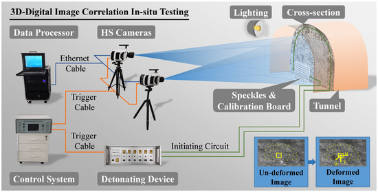
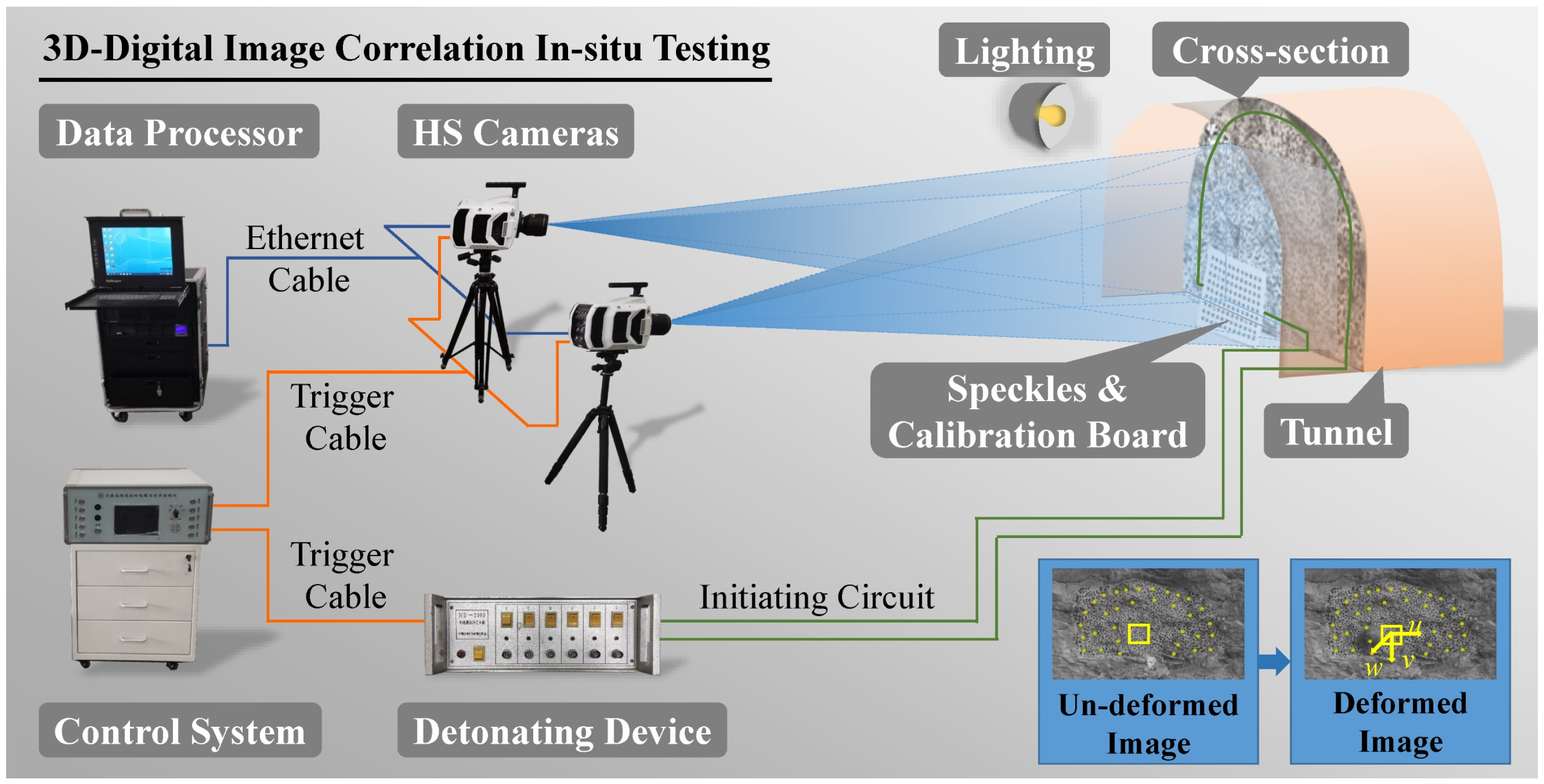
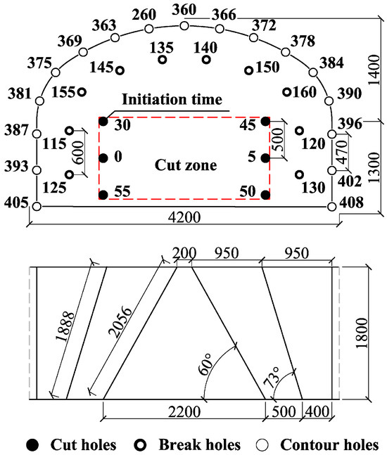
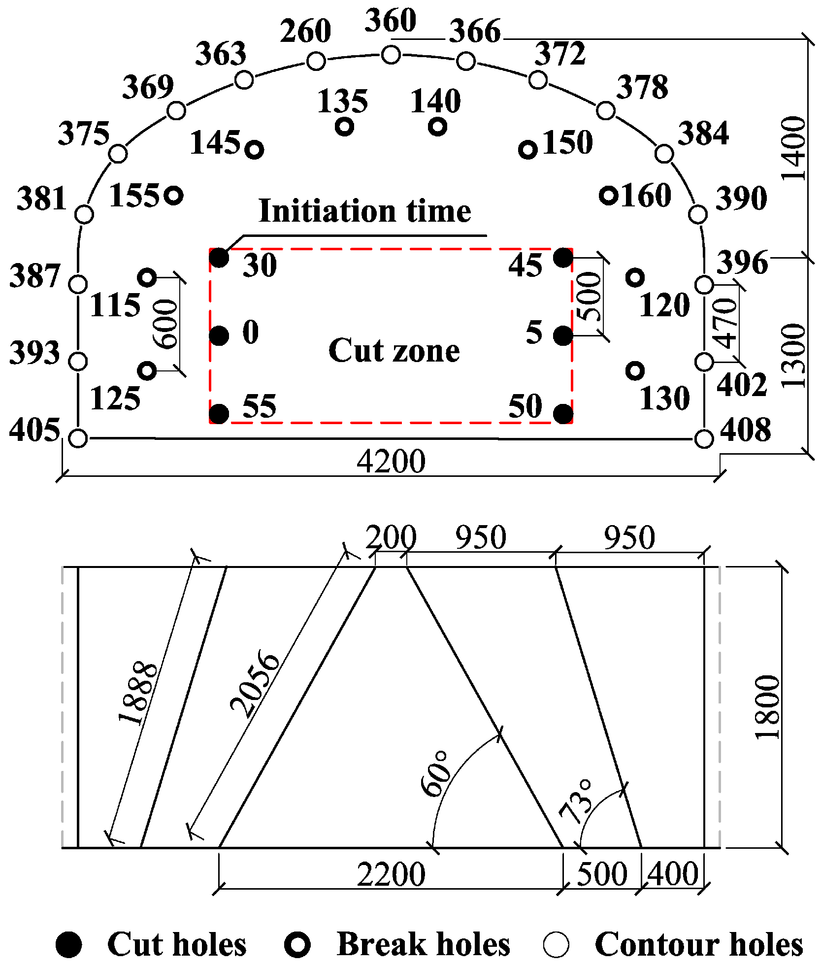
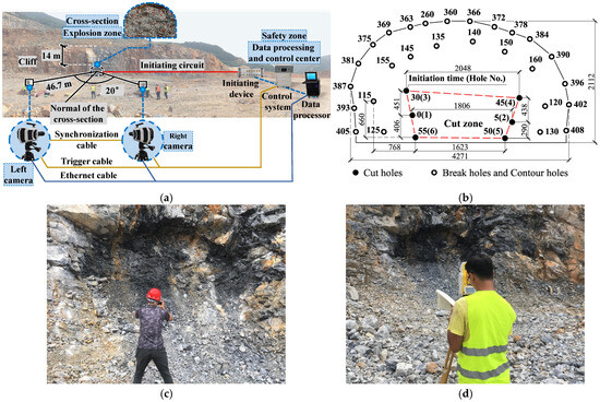
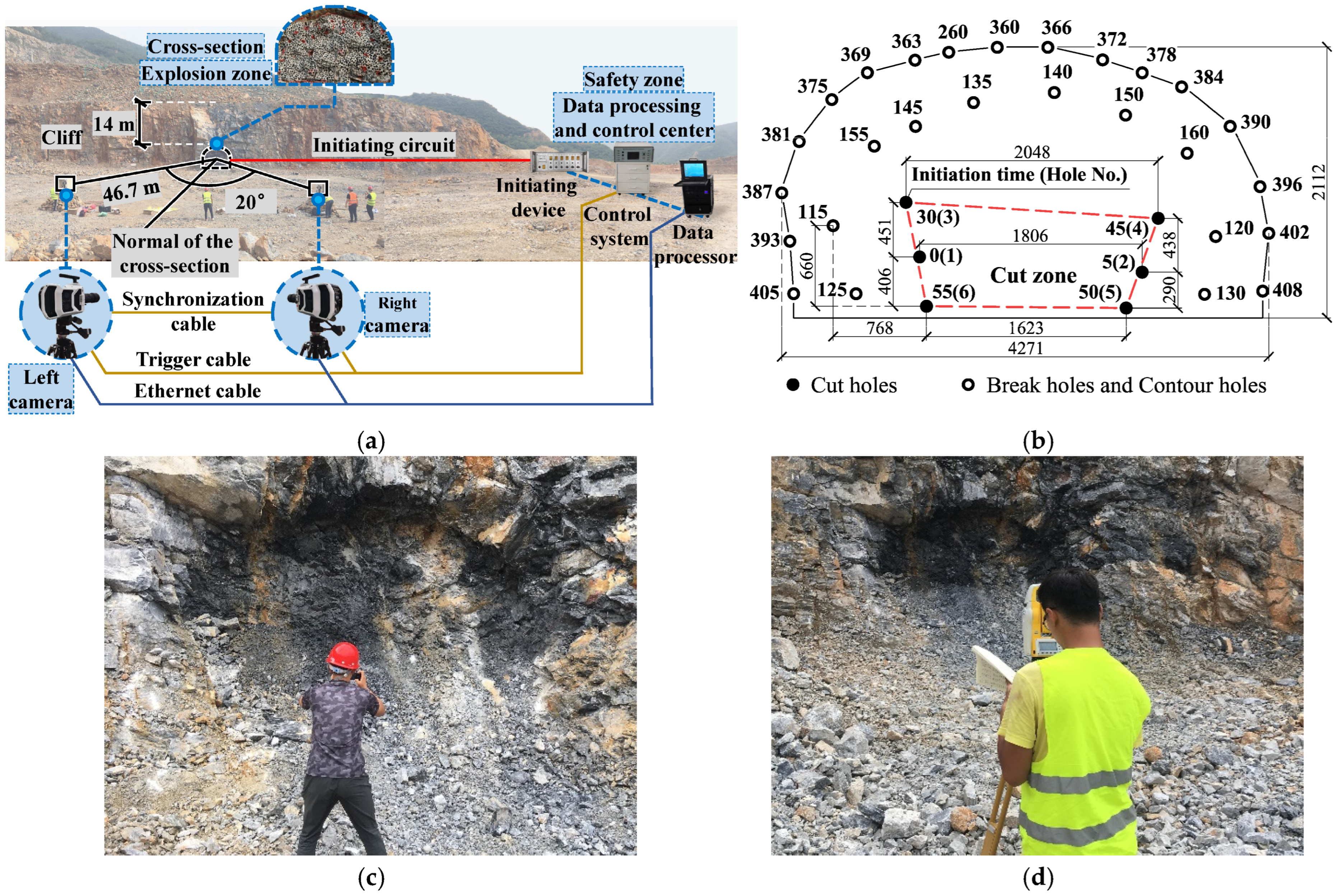
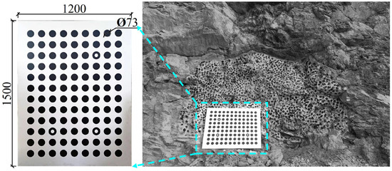
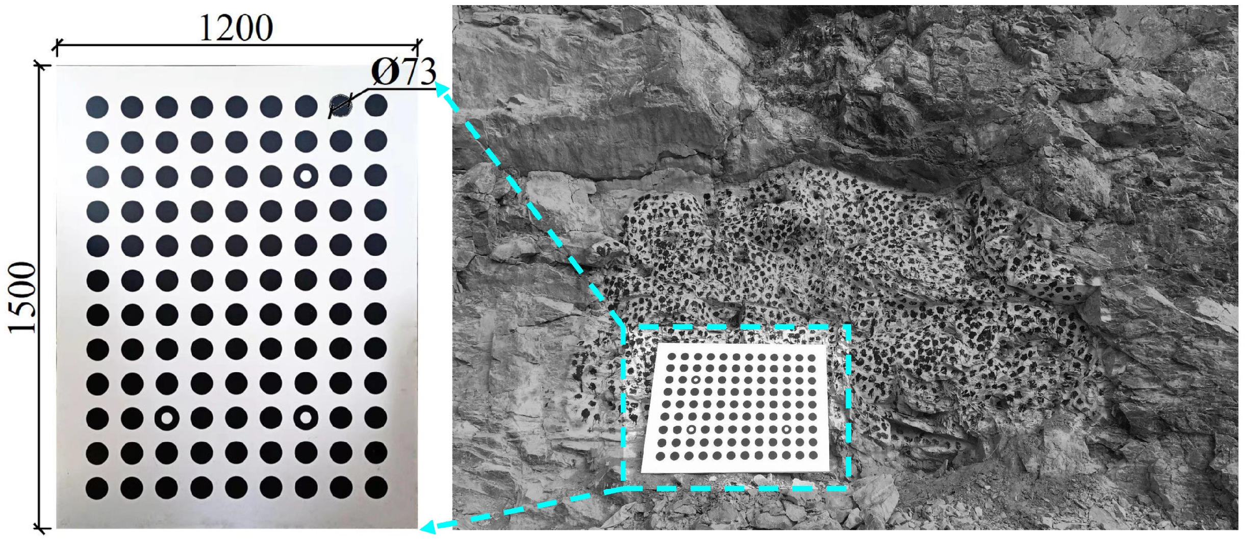
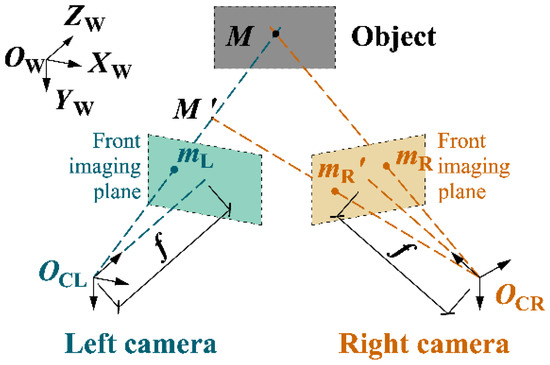
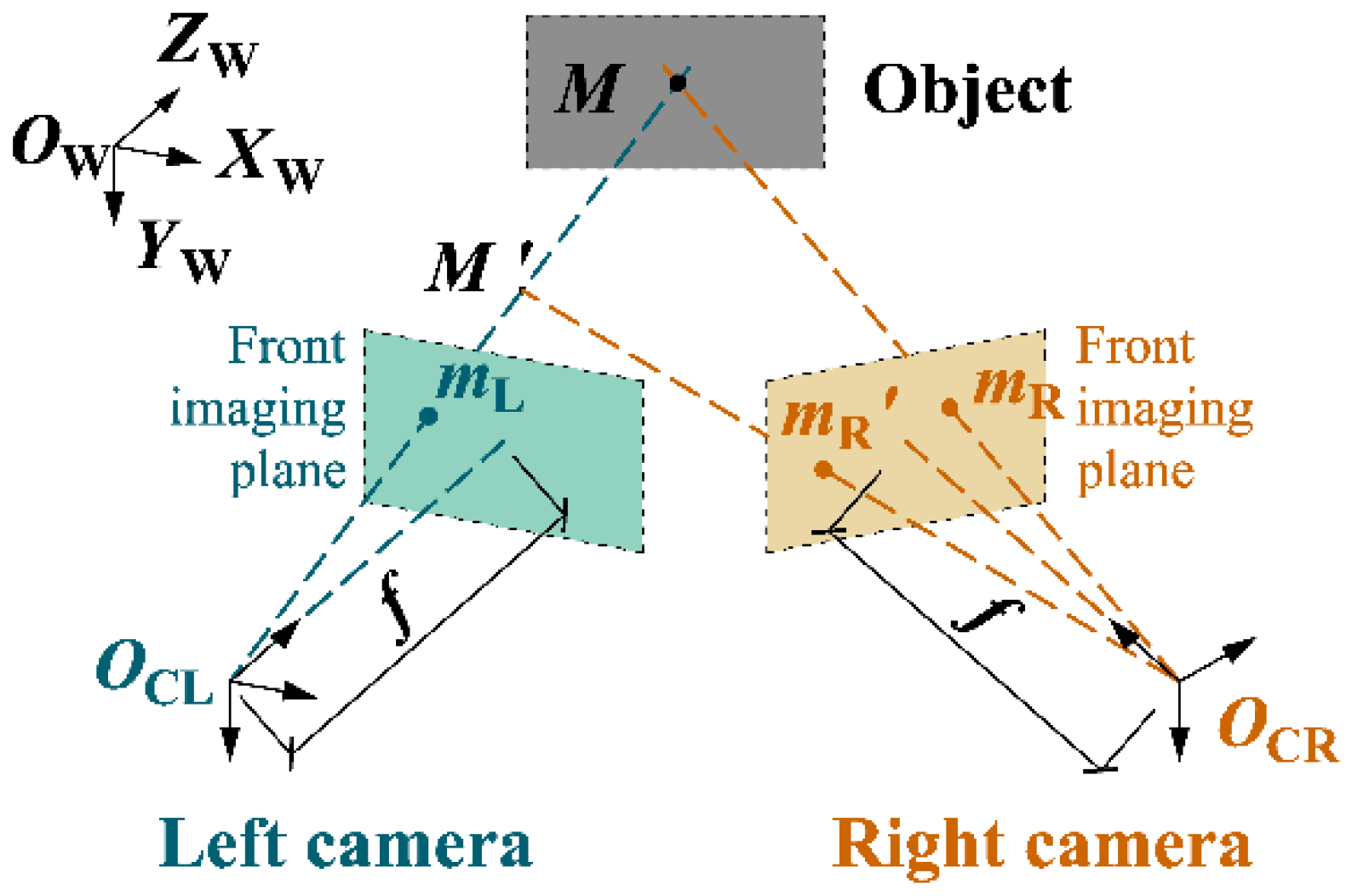
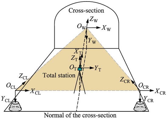
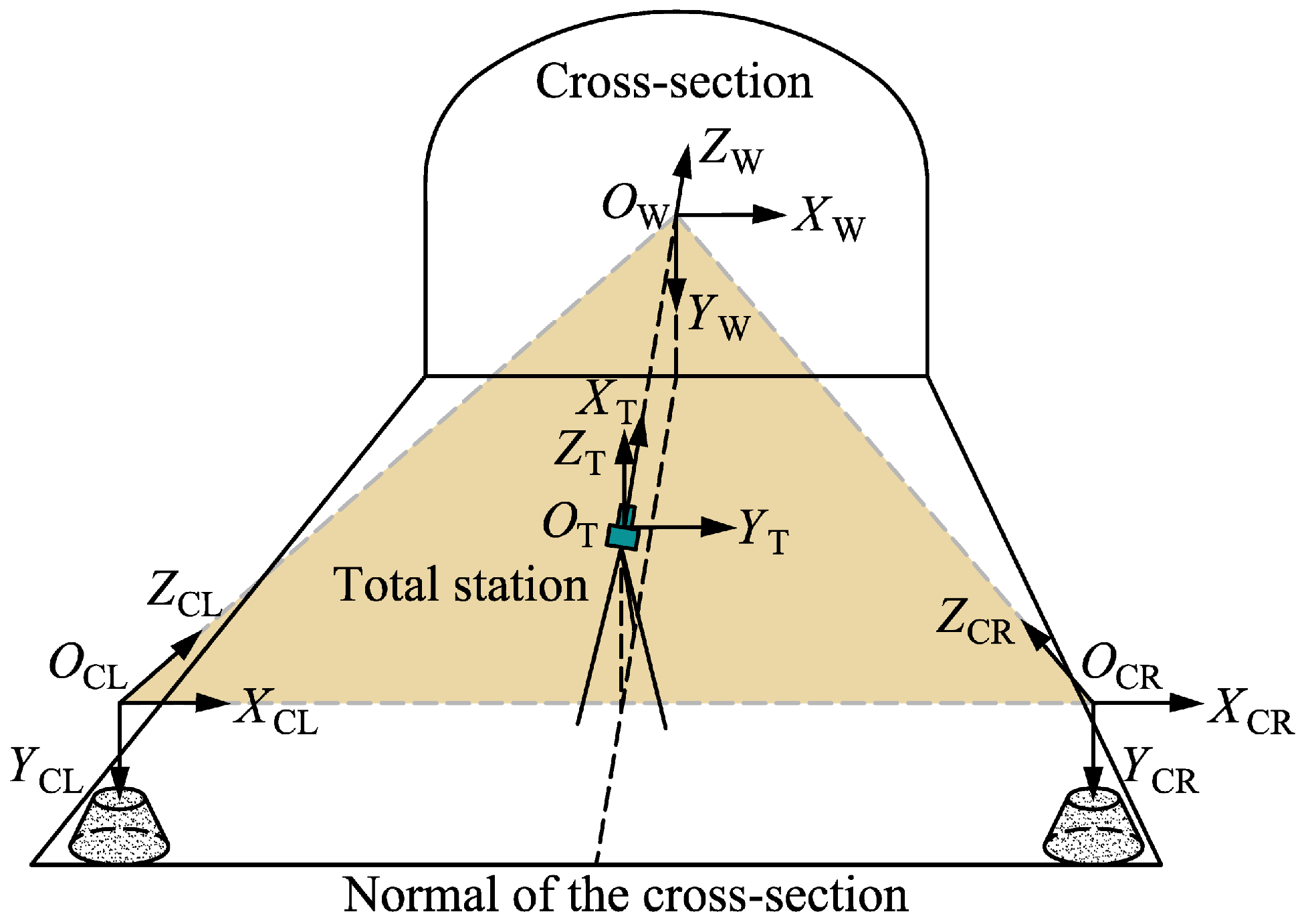
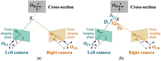
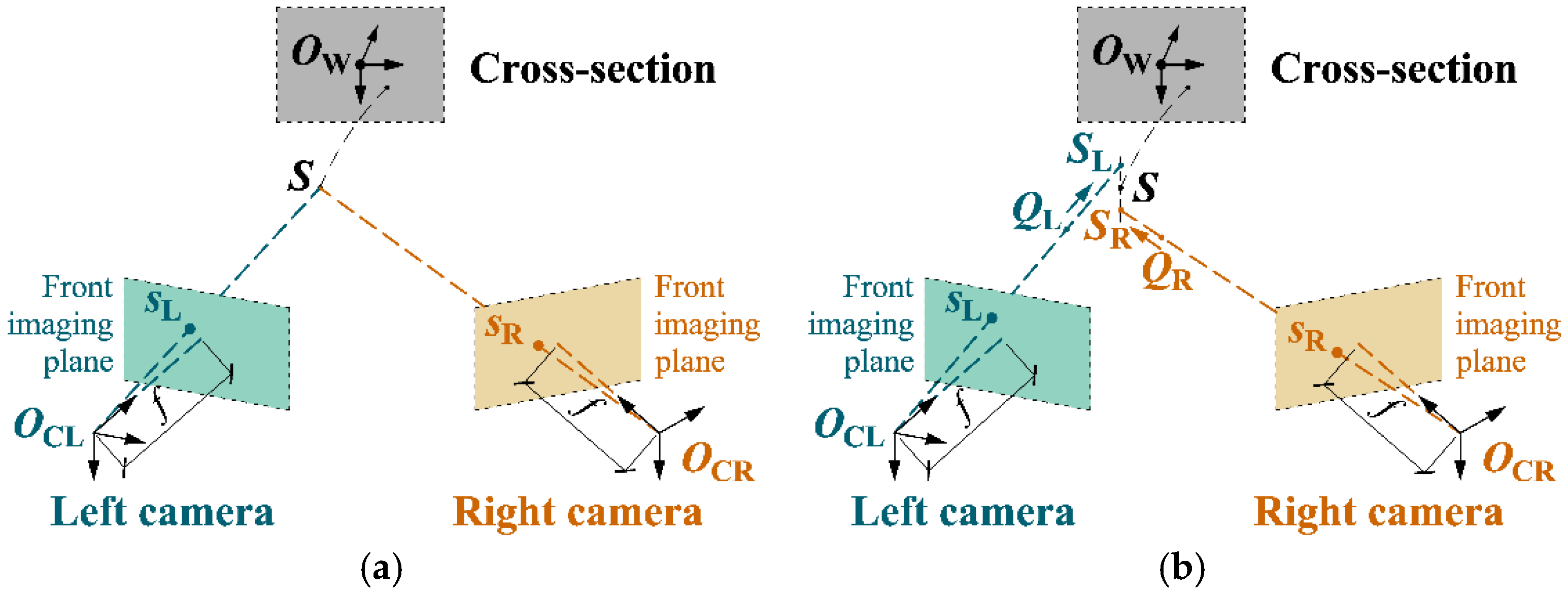
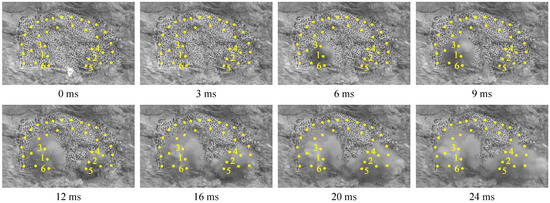
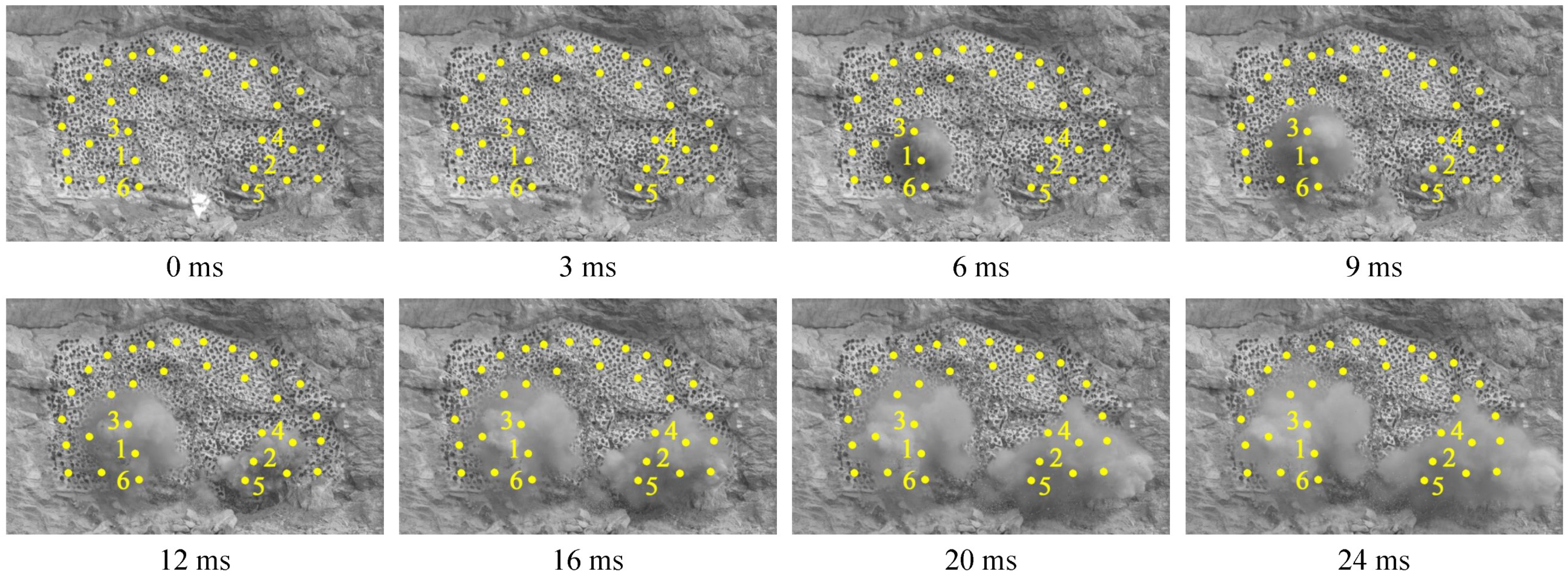
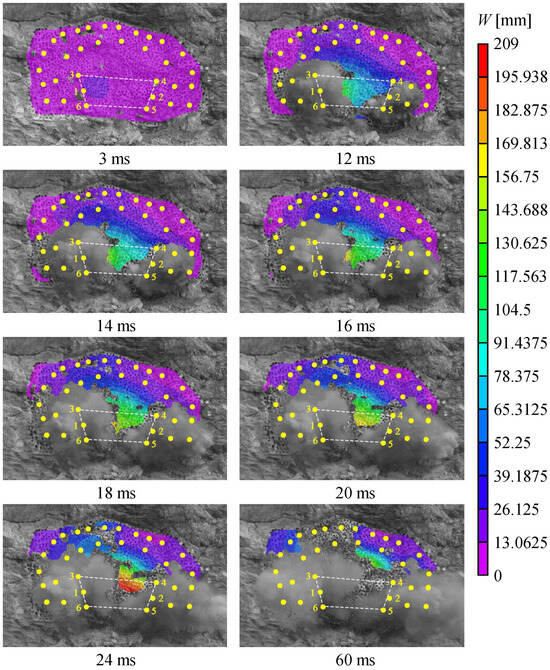
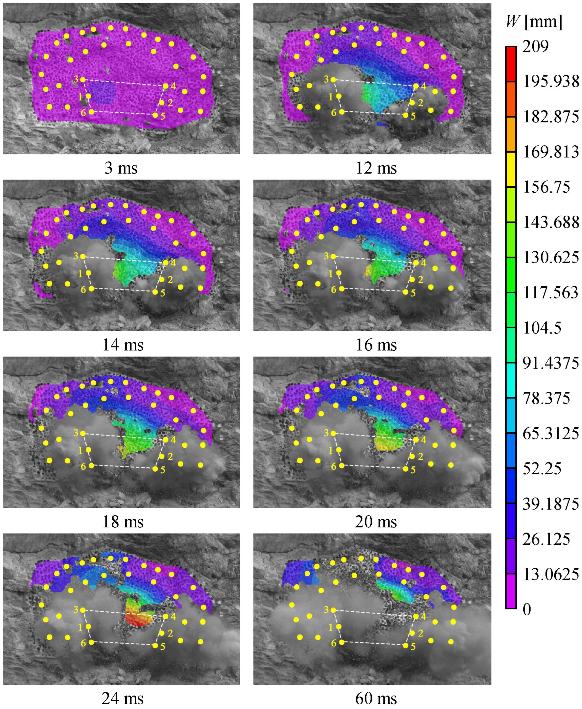
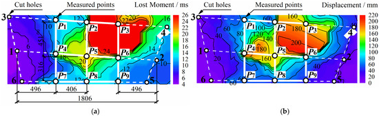
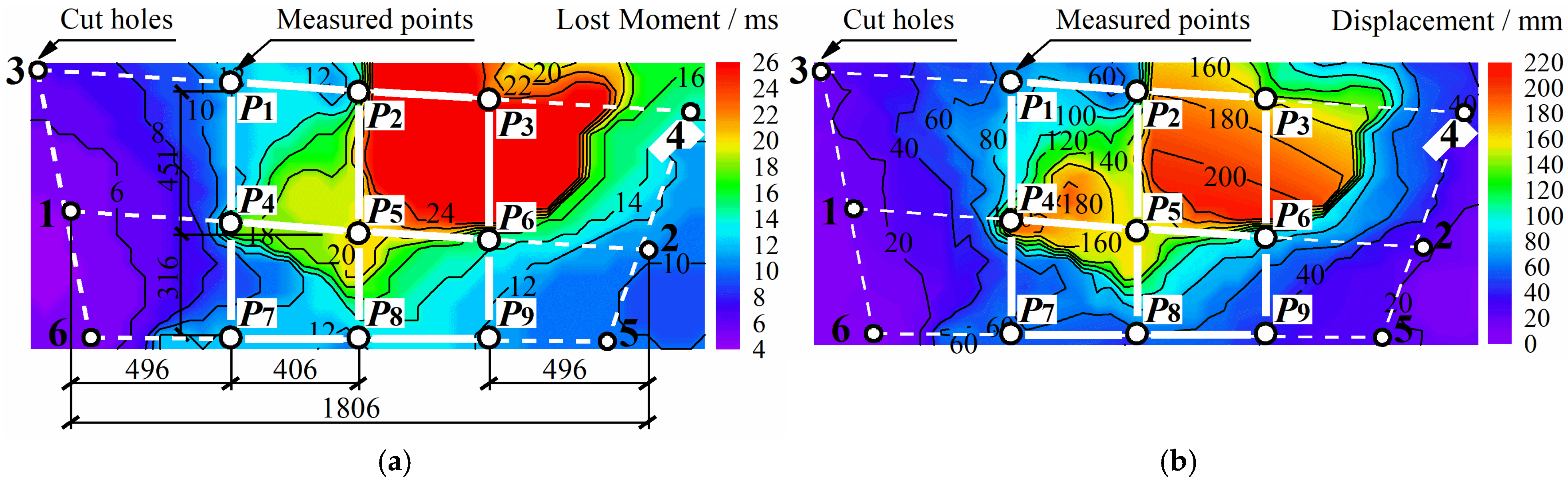
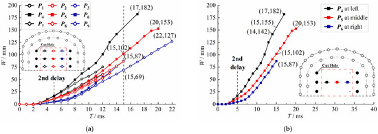
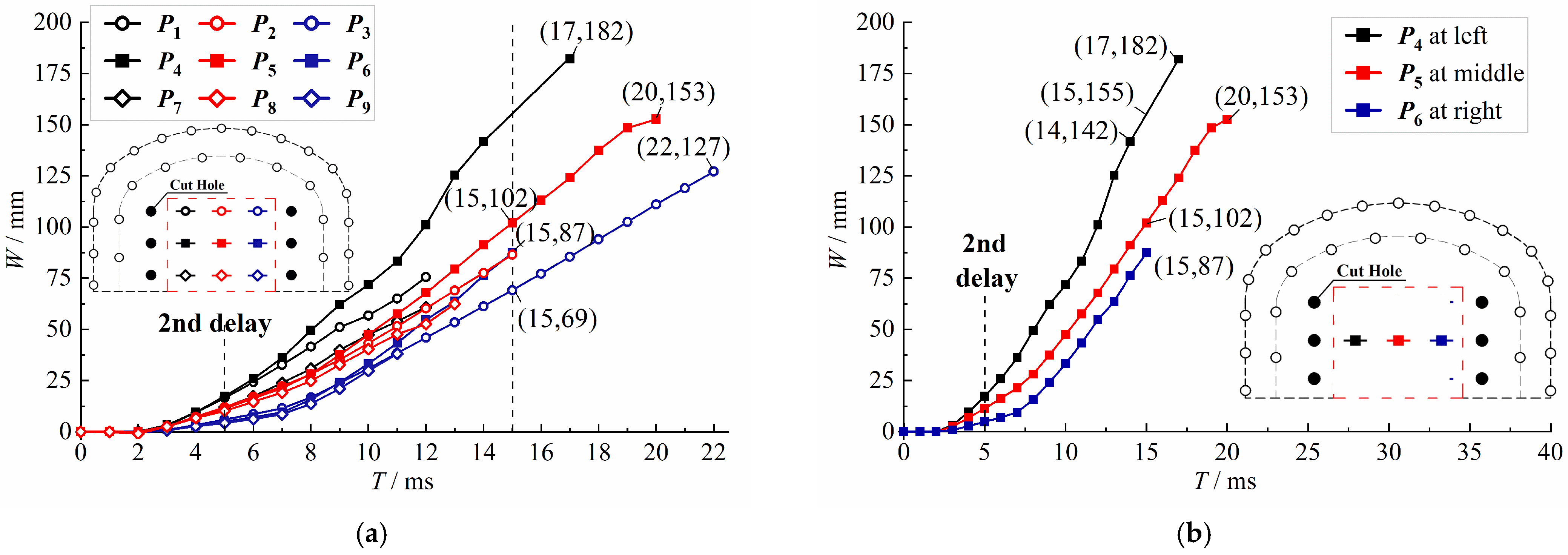
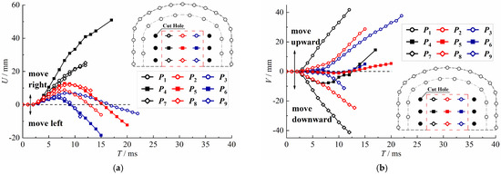
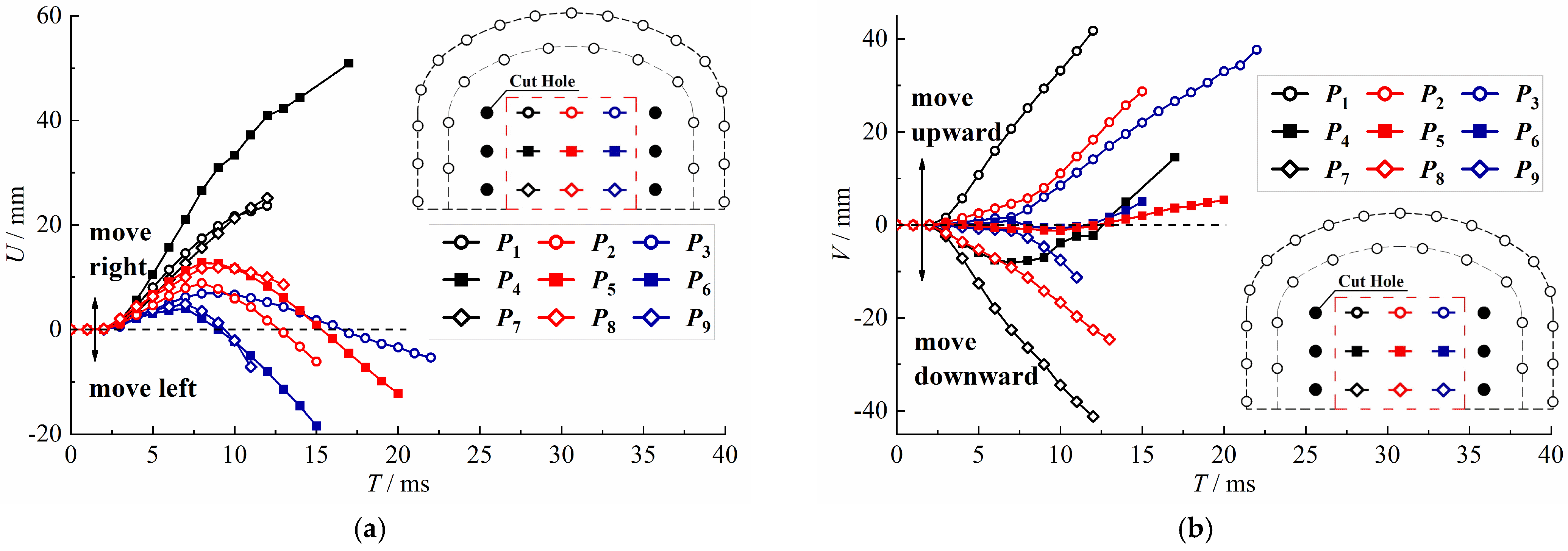
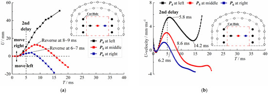
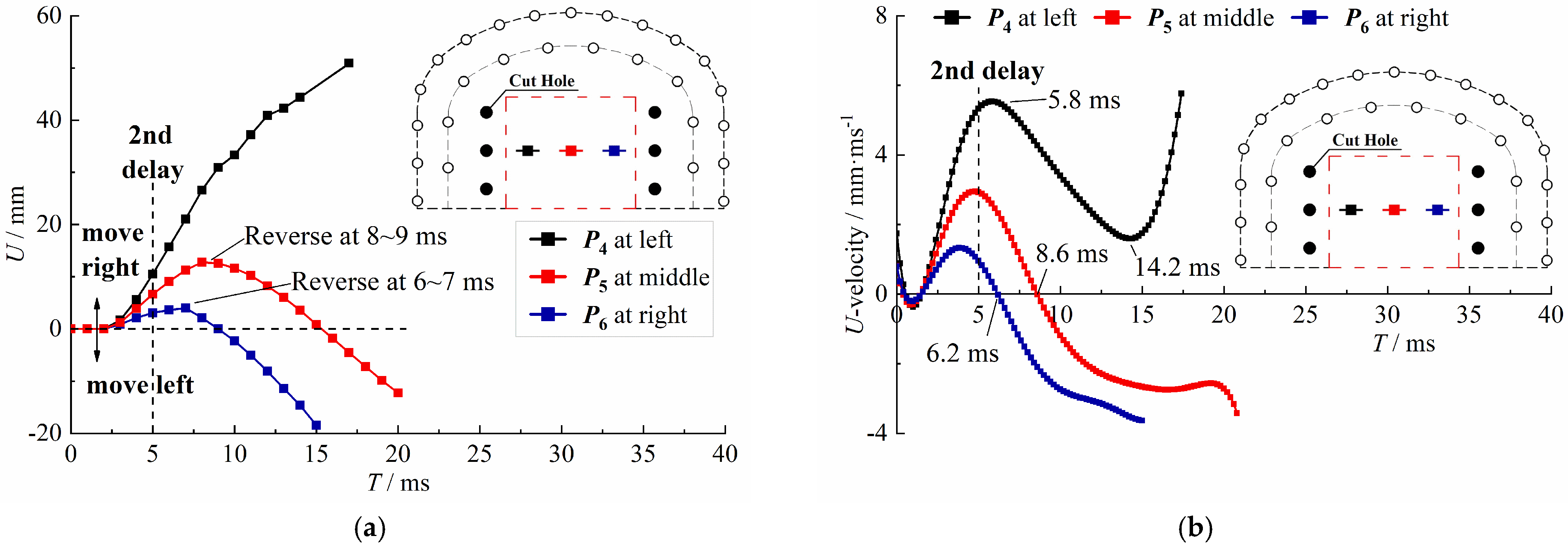
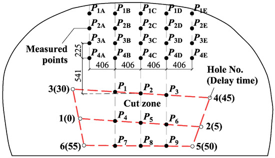
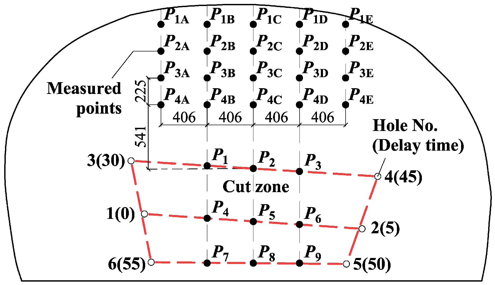
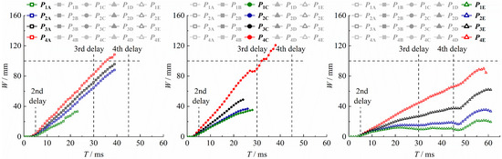
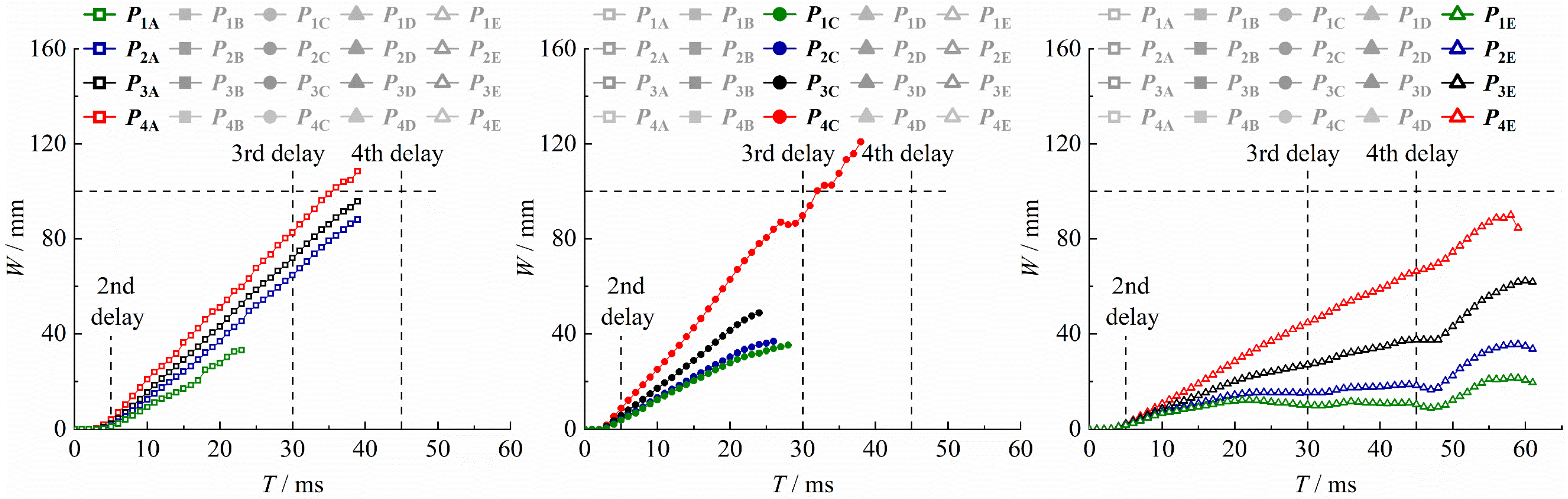
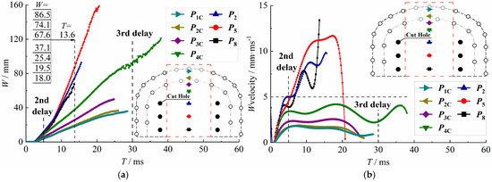
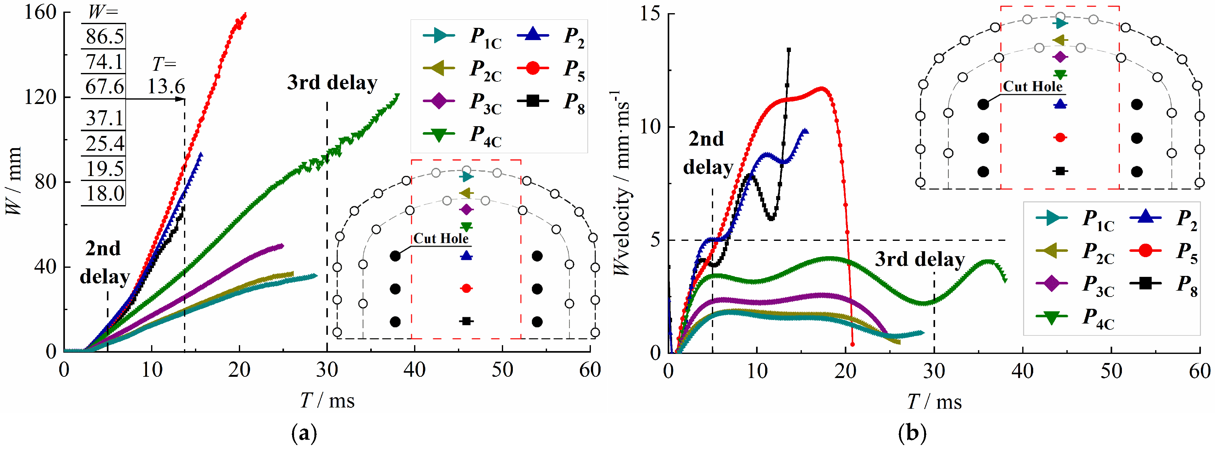
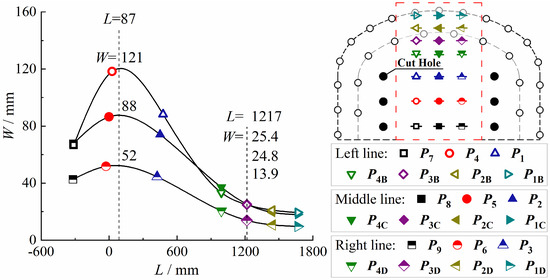
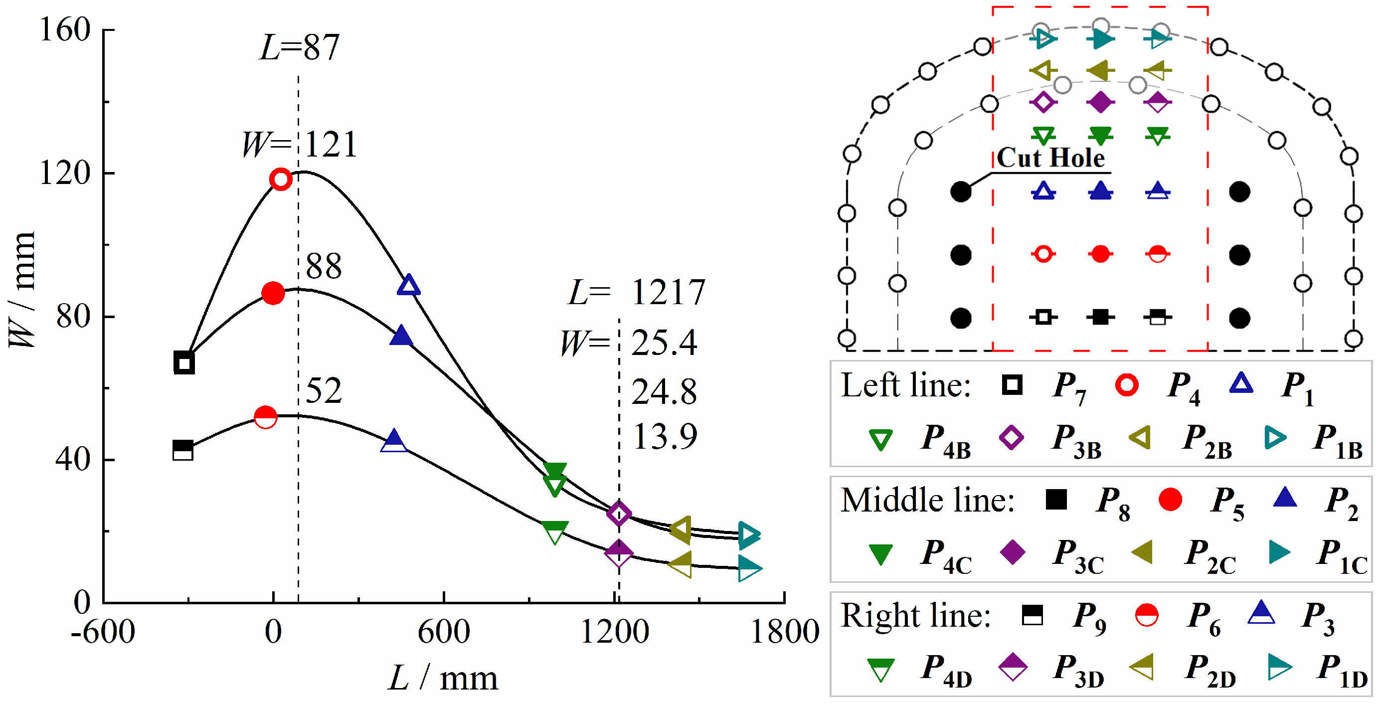
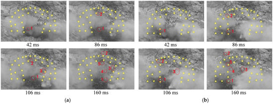
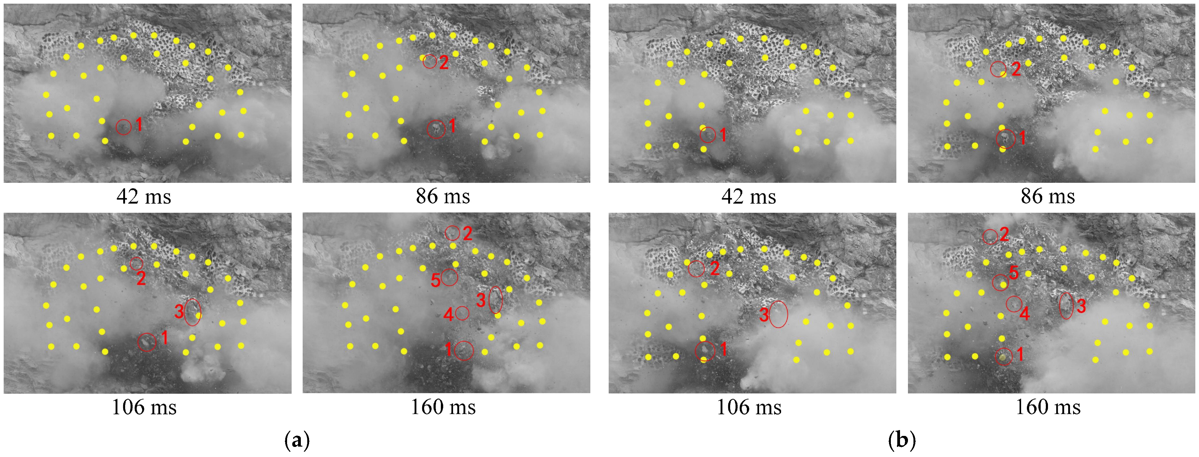
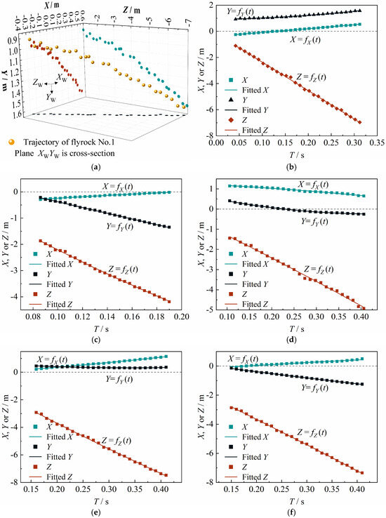
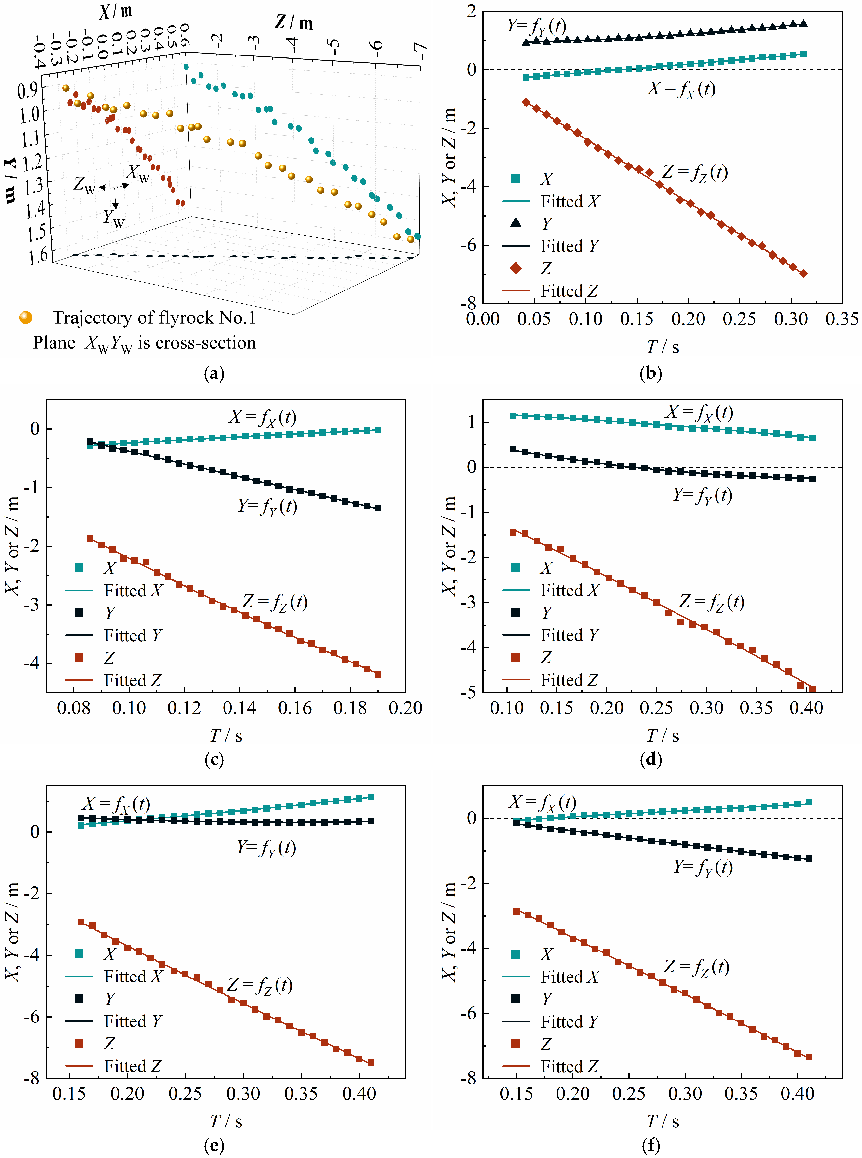
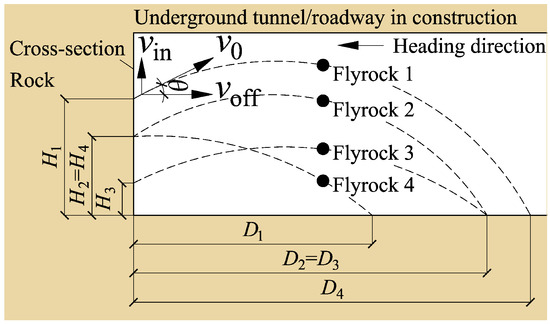
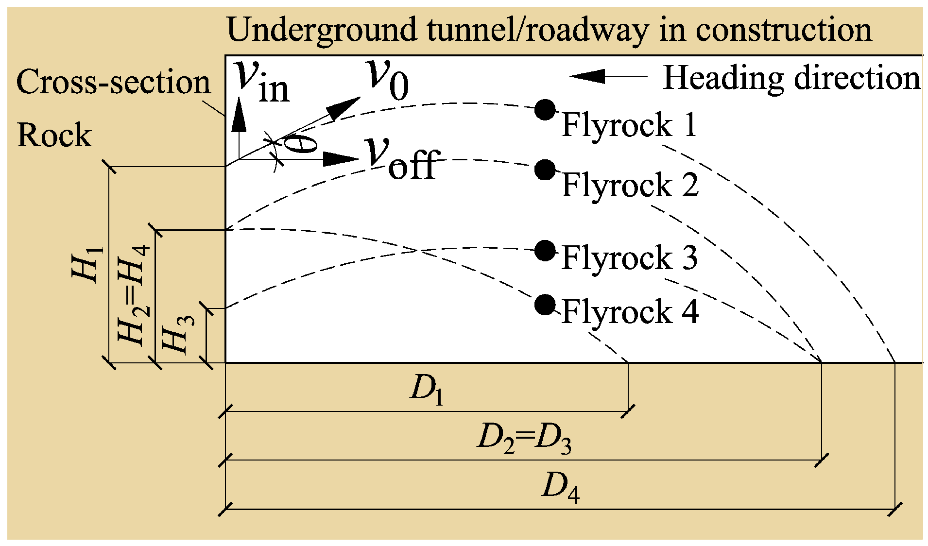
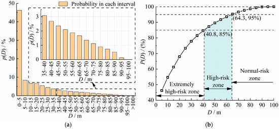
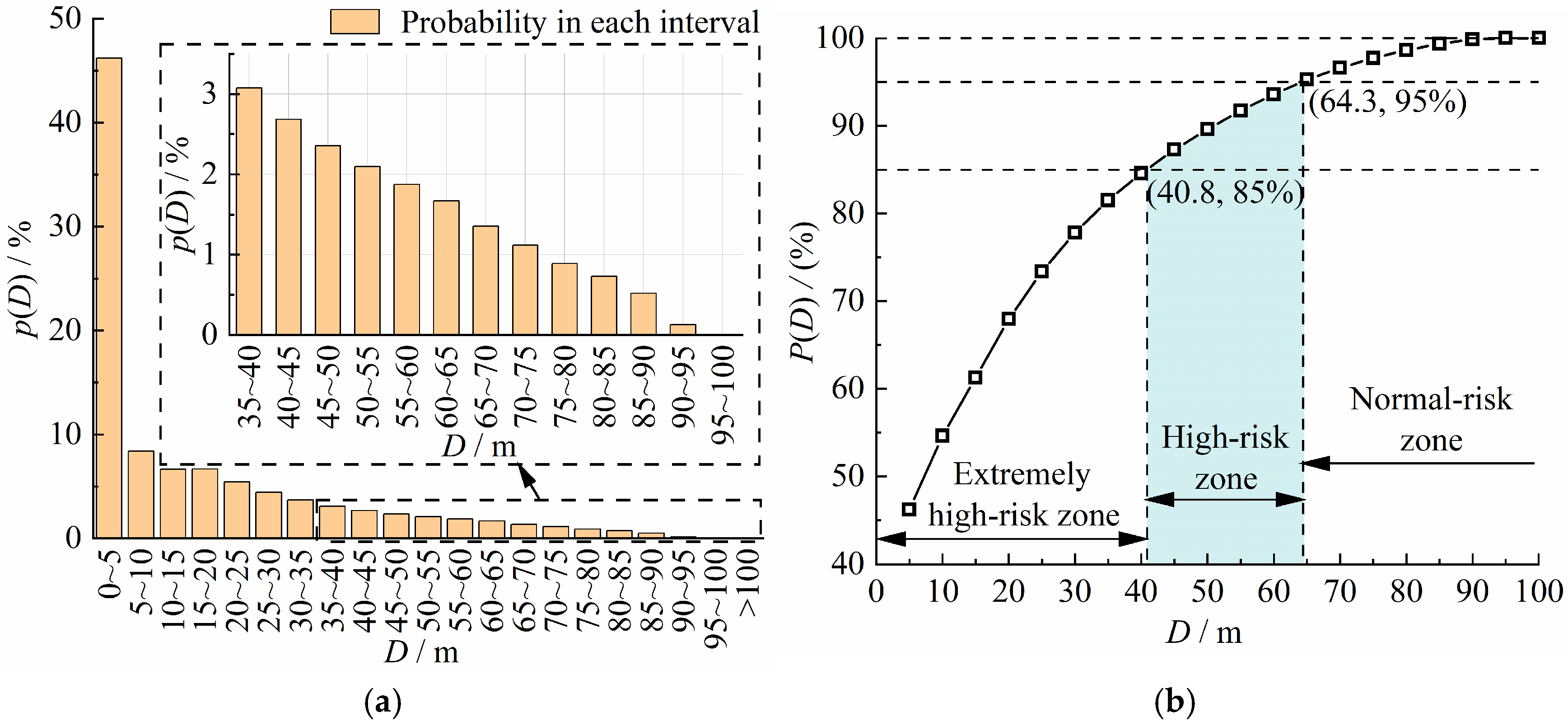

Disclaimer/Publisher’s Note: The statements, opinions and data contained in all publications are solely those of the individual author(s) and contributor(s) and not of MDPI and/or the editor(s). MDPI and/or the editor(s) disclaim responsibility for any injury to people or property resulting from any ideas, methods, instructions or products referred to in the content. |
© 2026 by the authors. Licensee MDPI, Basel, Switzerland. This article is an open access article distributed under the terms and conditions of the Creative Commons Attribution (CC BY) license.