Study of Methane Production Kinetics in Anaerobic Digesters Using the Monod Model and Neural Networks

Abstract

This study, conducted in the Ecuadorian Andes, evaluated the anaerobic co-digestion of local crop residues (amaranth and quinoa) with llama, vicuña, and pig manure to analyze methane production kinetics. The raw materials were characterized by proximate, elemental, and structural analyses, and biogas volume and the CH₄ fraction were monitored daily. The Amaranth-vicuña and Amaranth-llama treatments reached 77.29 ± 5.63 and 64.62 ± 3.62 mL biogas/g VS and 36.20 ± 7.29 and 31.78 ± 3.62 mL CH₄/g VS, respectively; in contrast, Quinoa-vicuña and Quinoa-llama produced only 1.04 ± 0.25 and 0.24 ± 0.03 mL CH₄/g VS. Monod-model parameters were estimated using an apparent formulation based on the methane production rate, and the kinetic behavior was compared with first-order, modified Gompertz, and modified logistic models. In addition, artificial neural networks (ANNs) were evaluated to predict the methane production curve from substrate characterization. Network 44, with a 13-15-10-1 architecture, yielded an overall R² = 0.998, validation R² = 0.997, and validation MSE = 0.415. Ten-times repeated five-fold cross-validation of the same architecture yielded R² = 0.985 ± 0.007 and RMSE = 1.21 ± 0.28 mL CH₄/g VS, supporting its interpolation capability within the experimental domain, although this does not demonstrate extrapolation to new substrate combinations. Overall, the proposed approach combines interpretable kinetic parameters with ANN-based prediction, but external validation with independent datasets is still required. The reported yields correspond to the specific production achieved in a low-cost batch system operated at room temperature and should not be interpreted as standardized biochemical methane potential (BMP) values.

1. Introduction

Bolívar Province, Ecuador, faces several challenges related to the energy transition. From September 2024 and for four months, the country experienced a severe energy crisis caused by a major drought and excessive dependence on hydroelectric power plants (69% of the electricity grid) [1]. Moreover, this is a rural region in which 32% of the economy is based on the agricultural sector (Ministry of Agriculture and Livestock, 2023 [2]). These activities generate large amounts of residues that have traditionally been managed by burning crop residues or applying untreated manure as fertilizer [3,4]).

Anaerobic digestion (AD) converts organic waste into biogas, an energy-rich gaseous mixture composed mainly of methane (CH₄) and carbon dioxide (CO₂) [5]. Thus, AD fits within circular-economy and waste-to-energy paradigms [6,7]. Although this technology has been used for decades in Andean regions, its application remains concentrated in small-scale household digesters [8]. These installations contribute to rural energy self-sufficiency, but their implementation remains limited by the scarcity of private initiatives and institutional support [9,10].

This study evaluates the anaerobic co-digestion (ACD) of lignocellulosic quinoa and amaranth residues with llama, vicuña, and pig manure. CH₄ production was analyzed using kinetic models and artificial neural networks (ANNs), with the aim of comparing the descriptive and interpretive capacity of simplified mechanistic models with the predictive capacity of data-driven models.

Biogas production kinetics have been described using Monod and Gompertz models, logistic functions, and first-order or exponential expressions. These models can represent the temporal evolution of the process and estimate parameters associated with rate, lag phase, or approach to maximum potential [11,12,13]. In anaerobic digestion, however, increasing the number of state variables and microbial populations rapidly increases model complexity; frameworks such as ADM1 represent multiple substrate fractions, intermediates, and microbial groups, whereas reduced models seek to retain a small number of identifiable parameters [14,15]. Therefore, model selection should reflect both data availability and the objective of the analysis.

The novelty of the proposed adaptation does not lie in modifying the fundamental Monod equation, but in defining an apparent saturation parameter referred to a substrate-availability variable inferred from the CH₄ formation rate when the residual concentration of the different substrates is not directly measured. Unlike studies that estimate K_s from concentrations of an identified soluble substrate or from multicomponent models, this approach uses only the methane time series and therefore provides K_s^ap as an empirical parameter specific to the test conditions. A second contribution is the integration of this interpretable kinetic characterization with an ANN fed by the physicochemical composition of the substrates. This combination makes it possible to contrast biological interpretation and prediction, two objectives that are commonly addressed separately.

Artificial intelligence (AI) has also provided tools for predicting and optimizing anaerobic digestion. Machine-learning algorithms can relate substrate composition and operating conditions to outputs such as biogas or methane yield [16,17]. Among them, ANNs are particularly suitable for representing nonlinear relationships between input and output variables [18,19,20].

One of the main challenges in configuring an ANN is selecting an architecture that is sufficiently flexible to represent the process without overfitting. The risk increases when the number of trainable weights and biases is large relative to the number of available patterns. In addition to architecture size, excessively prolonged training may fit experimental noise. For this reason, data are separated into training, validation, and test sets, and the mean squared error (MSE) is monitored. Training is stopped when the validation MSE ceases to improve, an early-stopping strategy that reduces, although it does not eliminate, the risk of overfitting [21,22].

ANNs can achieve high goodness of fit by capturing nonlinear patterns, but their coefficients do not have the direct biological interpretation of parameters such as μ_max, K_s, or lag time [23,24]. Moreover, their generalization capability depends on the size and diversity of the dataset. In AD, variability in substrates, temperature, pH, organic loading, and analytical procedures makes it difficult to transfer a network trained on one system to different conditions. Therefore, performance during training or in a random validation partition should not automatically be interpreted as evidence of external validity.

The main objective of this study was to compare traditional kinetic approaches and ANN-based models for describing and predicting methane production during the ACD of lignocellulosic residues with Andean manures. Specifically, the aims were to: (i) characterize the raw materials and quantify biogas and CH₄ production; (ii) estimate μ_max and an apparent saturation constant K_s^ap using a product-data-based adaptation of the Monod model; (iii) compare curve shape using first-order, modified Gompertz, and modified logistic models; and (iv) develop an ANN and explicitly assess its risk of overfitting through internal validation and cross-validation.

2. Materials and Methods

2.1. Location

Laboratory analyses were carried out between September 2024 and February 2025 at the Research Laboratories of Universidad Estatal de Bolívar, in Guaranda, in the Andean region of Ecuador. The city is located at 2622 m a.s.l. and has a temperate climate, with average temperatures ranging from 7 to 22 °C [25].

2.2. Substrates

The raw materials used were llama (Lama glama), vicuña (Vicugna vicugna), and guinea pig (Sus scrofa domesticus) manure, together with quinoa (Chenopodium quinoa) and amaranth (Amaranthus caudatus) crop residues. All materials were obtained from local farmers and livestock producers. The lignocellulosic residues were dried at room temperature for one week, manually chopped, and then milled to a particle size of 2–3 mm. Pelletized llama and vicuña manure was manually homogenized with a mortar and pestle. The substrates were stored in a dry, dark place until use.

2.3. Inoculum

Liquid inoculum from an anaerobic digester installed at the El Laguacoto II Campus of Universidad Estatal de Bolívar was used. The sample was collected in a clean plastic container and stored under dry, dark conditions until the digesters were assembled. Total solids (TS) and volatile solids (VS) of the inoculum were determined using Standard Methods 2540B and 2540E (APHA) [26].

2.4. Substrate Characterization

Proximate, elemental, and structural analyses of the substrates were performed. Moisture, VS, and ash contents were determined according to UNE-EN ISO 18134-2:2024 [27], UNE-EN ISO 18123:2023 [28], and UNE-EN ISO 18122:2023 [29]. Fixed carbon (CF) was calculated by difference using Equation (1) [30]. In Equation (1), VS denotes the volatile-solids content of the sample, expressed as a percentage on a dry basis (% d.b.; g/100 g dry sample).

$$CF=100-VS-A_d$$

(1)

where CF is fixed carbon (% on a dry basis), VS is the volatile-matter content (% on a dry basis), and A_d. is the ash content (% on a dry basis).

Elemental analysis was performed using a Vario Macro Cube elemental analyzer (Elementar Analysensysteme GmbH, Langenselbold, Germany). according to UNE-EN ISO 16948:2016 [31]. The C, H, N, and S contents and the C/N and C/H ratios were determined. Oxygen content was calculated by difference using Equation (2):

$$O_d=100-C_d-H_d-N_d-S_d-A_d$$

(2)

where $O_d$, $C_d$, $H_d$, $N_d,$ $S_d$, and $A_d$ represent the percentages of oxygen, carbon, hydrogen, nitrogen, sulfur, and ash, respectively, on a dry basis.

Structural analysis was performed only on the lignocellulosic residues using an ANKOM2000 fiber analyzer (ANKOM Technology, Macedon, NY, USA). Neutral detergent fiber (NDF), acid detergent fiber (ADF), and lignin were determined following the manufacturer’s protocols [32], based on Van Soest et al. [33]. Cellulose and hemicellulose contents were calculated from these results.

2.5. Digester Setup

A low-cost batch digester was reproduced at laboratory scale, without agitation and operated at room temperature, with a final TS content of 8–12% [34,35]. Six combinations of one manure and one crop residue were prepared. In each mixture, each co-substrate contributed 50% of the added VS. Each treatment was performed in triplicate, and three blanks containing inoculum and water were included.

Amber glass bottles with a total volume of 310 mL and a working volume of 60% (186 mL) were used. The substrate amount was calculated considering: (1) the working volume of the digester; (2) a 50:50 VS contribution from the two co-substrates; and (3) a final TS content of 8–12%. The amounts were determined using Microsoft Excel Solver. The working volume was completed with inoculum and, for the blanks, with the mean inoculum volume used in the treatments and water to 186 mL. Table 1 summarizes the amount of each component introduced into the digesters. For each co-digestion treatment, the amounts of manure and lignocellulosic residue were calculated so that each co-substrate contributed 50% of the added substrate VS. Therefore, the value reported in the last column corresponds to the VS contributed individually by the manure and by the lignocellulosic residue; the total VS supplied by the two co-substrates is twice this value. The different masses required among treatments result from differences in the TS and VS contents of the raw materials. Inoculum was subsequently added to complete the established working volume of 186 mL. No additional water was required in the co-digestion treatments, whereas the blank contained 134.5 mL of inoculum and 51.5 mL of water to reach the same working volume. Once assembled, the digesters were closed with rubber stoppers, sealed, and incubated at room temperature for 45 days.

Table 1. Amounts of substrates added to each digester.

Treatment	Manure (g)	Lignocellulosic Residue (g)	Inoculum (mL)	Water (mL)	VS Contribution of Each Co-Substrate (g VS)
Amaranth-vicuña	11.53	8.52	141	-	6.08
Amaranth-llama	21.70	9.13	125	-	6.52
Amaranth-pig	37.37	9.52	117	-	6.79
Quinoa-vicuña	11.41	8.02	154	-	6.01
Quinoa-llama	21.02	8.59	139	-	6.44
Quinoa-pig	36.90	8.95	131	-	6.71
Blank	-	-	134.50	51.50	-

The experimental design was deliberately conceived as a simulation of a low-cost rural batch digester rather than as a standardized biochemical methane potential (BMP) test. Consequently, controlled mesophilic conditions and a positive reference substrate for certifying inoculum activity were not used. BMP protocols recommend positive controls and specific inoculum-activity criteria to estimate a maximum potential that is comparable among laboratories [36]. Therefore, the results of the present study are interpreted as specific yields obtained under the tested operating conditions and not as the maximum biochemical methane potential of the substrates.

2.6. Biogas Measurement

Gas was measured daily for 45 days using a three-way valve connected to a 0.8-mm hypodermic needle, a 60-mL syringe, and a Delta OHM HD2124.2 digital manometer (Delta OHM S.r.l., Padova, Italy). Biogas was withdrawn until the internal pressure equaled atmospheric pressure (0.742 ± 0.002 atm). The recovered gas was analyzed with a BIOGAS 5000 portable biogas analyser (Geotech, QED Environmental Systems, Coventry, UK) to determine CO₂, CH₄, O₂, and H₂S. CO₂ and CH₄ (% v/v), H₂S (ppm), and O₂ (% v/v) values were recorded.

For subsequent data processing, biogas volume was expressed under standard conditions (25°C, 1 atm). Daily pressure data were corrected using Equation (3), as proposed by several authors, including Meneses-Quelal et al. [37]:

$$V_{BIOGAS}\left(STP\right)={\displaystyle \frac{P_{ABS}{·V}_G{·T}_{STP}}{P_{STP}·T_1}}$$

(3)

where $V_{BIOGAS}\left(STP\right)$ is the final biogas volume under standard conditions; $P_{ABS}$ is the pressure increase caused by digester overpressure, calculated as the difference between the measured pressure and atmospheric pressure (atm); $P_{STP}$ is the pressure under standard conditions (1 atm); $T_1$ is the experimental temperature (K), for which 18 °C was taken as the mean laboratory temperature; $T_{STP}$ is the temperature under standard conditions (298 K); and $V_G$ is the digester headspace volume (0.124 L).

With respect to altitude,$P_{ABS}$ was used in the calculation as the pressure increase relative to the local atmosphere, i.e., $\Delta P=P_{int}-P_{atm},$ rather than as the reactor’s total absolute pressure. The measured local atmospheric pressure was 0.742 ± 0.002 atm; thus, the lower barometric pressure associated with the site at 2622 m a.s.l. was explicitly incorporated into the calculation. Subsequent conversion to 25 °C and 1 atm was performed using the ideal-gas law, so no additional altitude-related volumetric factor was required.

Continuous laboratory-temperature records were not available, and 18 °C was used as the mean value for normalization. This absence limits the temporal resolution of any thermal effect on biological rates and is recognized as a study limitation. Nevertheless, for the purely volumetric correction, an illustrative deviation of ±5 °C around 18 °C would change the normalized volume by approximately ±1.7%, a magnitude much smaller than the differences in CH₄ yield observed among treatments.

The volume of each gaseous component was obtained by multiplying the corrected biogas volume by its volumetric fraction. For treatment comparisons, results were normalized by the total VS in the mixture and expressed as mL/g VS.

2.7. Comparison Among Treatments

Differences among treatments were analyzed by one-way analysis of variance (ANOVA) followed by Tukey’s HSD test in RStudio version 2026.07.1. The significance level was set at α = 0.05. Where applicable, results are presented as mean ± standard deviation (SD) of three independent replicates (n = 3). Tables or figures presenting only descriptive parameters or fit metrics are explicitly identified as such and do not include inferential significance levels.

2.8. Fitting the Experimental Data to the Monod Model

Parameters were estimated from the Monod (1949) [38] model, Equation (4). Because a single residual substrate concentration was not measured during ACD, an apparent formulation based on the CH₄ formation rate was developed. This formulation is not intended to replace the actual physicochemical concentration of each substrate fraction, but rather to construct a proxy variable for metabolic availability from an experimentally measured product variable.

The aim of this section is not to construct a complete mechanistic model of anaerobic digestion through simultaneous differential balances of substrate, biomass, and intermediates, but to obtain comparable kinetic descriptors from the variables actually measured. A complete differential system would require independent time series of S(t), X(t), and intermediate species, in addition to initial conditions and yield/decay parameters. In this experiment, initial substrate characterization and a gas-production time series are available, but dynamic measurements of biomass, residual substrate, or volatile fatty acids (VFAs) are not. Simultaneously fitting a multivariable model with those states would therefore introduce parameters that are not identifiable from the available information. A reduced apparent formulation was therefore deliberately adopted for within-experiment comparison, and its interpretation should not be extended to a complete mechanistic simulation of the process [14,15].

$$\mu ={\displaystyle \frac{{\mu }_{max}·S}{K_S+S}}$$

(4)

where μ is the specific growth rate, μ_max is its maximum value, S is the available substrate concentration, and $K_S$ is the half-saturation constant, defined as the concentration of S at which μ = μ_max/2 [39].

The exponential growth model in Equation (5) was used to determine the maximum specific growth rate (${\mu }_{max}$).

$$X=X_0\cdot e^{\mu t}$$

(5)

where $X$ is the biomass concentration in the bioreactor, $X_0$ is its initial value, μ is the specific growth rate, and $t$ is time.

During the exponential phase, with substrate in excess ($K_s<<S$), $\mathsf{\mu }$ can be approximated as ${\mathsf{\mu }}_{\max }$ [40]. Likewise, under an approximately constant product/biomass yield over the selected interval, the increase in CH₄ reflects the activity of the methanogenic consortium. Under these conditions, Equation (6) was used to describe apparent product growth:

$$M=M_0\cdot e^{{\mathsf{\mu }}_{\max }·t}$$

(6)

where M is the cumulative amount of methane, $M_0$ is its value at the beginning of the exponential phase, μ_max is the maximum specific rate, and t is time. In this expression, $M_0$ is not the methane amount at the time of inoculation. For each replicate, it was defined as the first strictly positive cumulative CH₄ value at the beginning of the selected exponential segment; equivalently, t represents the elapsed time from the start of that segment. Therefore, Equation (6) is not applied with $M_0=0$ and is not intended to describe process start-up from an absence of product. The preceding lag phase is treated separately using the model in Section 2.9.

Equation (6) was linearized using natural logarithms to obtain Equation (7), in the linear form y = mx + n. The slope of $ln\left(M\right)$ versus time corresponds to $\mathsf{\mu }\max$.

The log-linear form was selected to provide a transparent estimate of the slope from the small number of observations belonging to each exponential segment and to apply exactly the same procedure to all replicates. This transformation preserves the kinetic slope of the exponential model but changes the error structure: fitting is performed on ln(M), which is equivalent to assuming a multiplicative error and may weight low values differently from direct nonlinear regression on the original scale. Consequently, μ_max is interpreted as an apparent descriptor of the selected segment rather than as a mechanistic parameter independent of the fitting procedure.

$$ln\left(M\right)={ln(M}_0)+{\mu }_{max}t$$

(7)

where the parameters are those defined for Equation (6).

The fit was performed separately for each replicate. Cumulative CH₄ points belonging to the exponential phase were selected, ln(M) was calculated, and linear regression against time was performed. The slope was taken as μ_max and R² as an indicator of goodness of fit. The mean μ_max for each treatment was then calculated, and ANOVA followed by Tukey’s HSD test (α = 0.05) was applied to compare treatments. Linear regression was performed by ordinary least squares (OLS) using the Microsoft Excel linear-trend function. The objective function was SSE = Σ_i[ln(M_i) − (b₀ + b₁t_i)]²; no iterative optimization algorithm was required. Slope b₁ was identified with μ_max and intercept b₀ with ln(M₀). R² was also recorded for each replicate.

Estimating K_s in the conventional Monod model requires knowledge of the available substrate concentration. In lignocellulosic ACD, several substrate fractions and microbial populations coexist and are linked through hydrolysis, acidogenesis, acetogenesis, and methanogenesis; therefore, a single concentration S does not adequately represent the system state [14]. From a macroscopic balance, the methane formation rate $r_M={\displaystyle \frac{\Delta M}{\Delta t}}$ is related to the consumption rate of the methanogenic precursor through an apparent yield. In this work, a proxy variable for substrate availability proportional to $r_M$ is therefore defined according to Equation (8). This approximation is empirical and is considered valid only within the experimental conditions analyzed.

$$S=a{\displaystyle \frac{∆M}{∆t}}$$

(8)

where ΔM is the increase in methane over the interval Δt and a is a proportionality constant. Accordingly, S in this transformation should be interpreted as an apparent availability variable rather than as the measured residual concentration of a specific chemical compound.

Substituting this proxy variable into Equation (4) gives Equation (9):

$$\mathsf{\mu }={\displaystyle \frac{{\mathsf{\mu }}_{\mathrm{m}\mathrm{a}\mathrm{x}}·\mathrm{a}\frac{∆\mathrm{M}}{∆\mathrm{t}}}{{{\mathrm{K}}_{\mathrm{S}}}^{\mathrm{a}\mathrm{p}}+\mathrm{a}\frac{∆\mathrm{M}}{∆\mathrm{t}}}}$$

(9)

where μ_max is the maximum specific growth rate, ΔM/Δt is the apparent methane formation rate, a is the proportionality constant, and K_s^ap is an apparent saturation constant referred to the product.

Because a cannot be identified independently without residual-substrate measurements, it is incorporated into the apparent parameter. Thus, the proposed adaptation is expressed by Equation (10). K_s^ap should not be interpreted as an intrinsic microorganism-substrate affinity constant or compared directly with K_s values obtained from concentrations of defined substrates; its utility is comparative among treatments evaluated under the same experimental protocol [15].

$$\mathsf{\mu }={\displaystyle \frac{{\mathsf{\mu }}_{\mathrm{m}\mathrm{a}\mathrm{x}}·\frac{∆\mathrm{M}}{∆\mathrm{t}}}{{{\mathrm{K}}_{\mathrm{S}}}^{\mathrm{a}\mathrm{p}}+\frac{∆\mathrm{M}}{∆\mathrm{t}}}}$$

(10)

where K_s^ap retains the apparent definition established in Equation (9), after absorbing the proportionality constant a into the half-saturation parameter.

Equation (10) was linearized by taking the reciprocal of its terms and rearranging them to obtain Equation (11). In this form, the intercept is 1/μ_max and the slope is K_s^ap/μ_max.

$${\displaystyle \frac{1}{\mathsf{\mu }}}=\left({\displaystyle \frac{{{\mathrm{K}}_{\mathrm{S}}}^{\mathrm{a}\mathrm{p}}}{{\mathsf{\mu }}_{\mathrm{m}\mathrm{a}\mathrm{x}}}}\right){\displaystyle \frac{1}{\frac{∆\mathrm{M}}{∆\mathrm{t}}}}+{\displaystyle \frac{1}{{\mathsf{\mu }}_{\mathrm{m}\mathrm{a}\mathrm{x}}}}$$

(11)

where 1/μ is plotted against Δt/ΔM; the slope is K_s^ap/μ_max and the intercept is 1/μ_max.

The apparent specific rate μ_i was calculated after the exponential phase, when μ < μ_max. Equations (12) and (13) were applied to two consecutive points:

$${\mathrm{M}}_{\mathrm{i}+1}={\mathrm{M}}_{\mathrm{i}}\cdot {\mathrm{e}}^{{\mathsf{\mu }}_{\mathrm{i}}·{{(\mathrm{t}}_{\mathrm{i}+1}-\mathrm{t}}_{\mathrm{i}})}$$

(12)

Therefore,

$${\mathsf{\mu }}_{\mathrm{i}}={\displaystyle \frac{1}{{\mathrm{t}}_{\mathrm{i}+1}-{\mathrm{t}}_{\mathrm{i}}}}\ln {\displaystyle \frac{{\mathrm{M}}_{\mathrm{i}+1}}{{\mathrm{M}}_{\mathrm{i}}}}$$

(13)

where t is time (d), i identifies the interval, μ_i is the apparent specific rate for the interval (d⁻¹), and M is cumulative methane (mL CH₄/g VS).

For replicates with a clearly identifiable stationary phase, μ_i was calculated using Equation (13) for intervals after the exponential phase. This selection makes it possible to describe the progressive decrease in the apparent methane formation rate as the system approaches stabilization or a process limitation.

When the stationary phase was not reached within 45 days, Equation (13) was applied to the last four experimental points. This criterion provides the minimum number of observations used in the linearization and should be considered an approximation; therefore, K_s^ap values for these treatments are interpreted with caution.

For each selected interval, Δt_i/ΔM_i was calculated, where Δt_i is the elapsed time between two consecutive measurements and ΔM_i is the corresponding increase in cumulative CH₄. This ratio is the inverse of apparent methane productivity: high values indicate lower CH₄ formation per unit time.

According to Equation (11), 1/μ_i was plotted against Δt_i/ΔM_i in Microsoft Excel and a linear regression was fitted for each replicate. The slope, intercept, and R² were recorded as goodness-of-fit indicators. This second fit was also performed by OLS in Excel, minimizing SSE = Σ_i[(1/μ_i) − (b₀ + b₁·Δt_i/ΔM_i)]², with b₀ = 1/μ_max and b₁ = K_s^ap/μ_max. The reciprocal transformation can amplify the influence of intervals with small ΔM; therefore, only intervals with positive CH₄ increments were used, and K_s^ap is interpreted comparatively and with caution.

K_s^ap was calculated from the slope and the previously estimated μ_max value for each replicate. This parameter apparently describes the relationship between process rate and CH₄ formation rate when a direct measurement of residual substrate is unavailable.

The relationship used between apparent substrate availability and CH₄ formation rate is therefore a model-closure hypothesis rather than an experimentally verified physicochemical proportionality. Mechanistic validation would require time series of residual substrate and intermediates, for example VFAs. Consequently, K_s^ap is used exclusively as an empirical comparative descriptor within this experiment and not as a measure of intrinsic microorganism-substrate affinity.

Replicate K_s^ap values were grouped by treatment and expressed as mean ± SD. Differences among treatments were evaluated by one-way ANOVA followed by Tukey’s HSD test in RStudio, with α = 0.05.

2.9. Fitting the Experimental Data to the Exponential Model

Although lag time ($t_{lag}$) is not a Monod parameter, it was estimated using Equation (14), derived from the exponential model and used to represent cumulative methane production M [12].

$${\mathrm{M}=\mathrm{Y}}_{\mathrm{P}/\mathrm{S}}·{\mathrm{X}}_0·{\mathrm{e}}^{\mathsf{\mu }\mathrm{m}\mathrm{a}\mathrm{x}(\mathrm{t}-{\mathrm{t}}_{\mathrm{l}\mathrm{a}\mathrm{g}})}$$

(14)

where Y_P/S is the product/substrate yield, X₀ is the initial biomass, μ_max is the maximum specific growth rate, and t_lag is the lag time.

The parameters $Y_{P/S}$·X₀, μ_max, and $t_{lag}$ were estimated by nonlinear regression using Microsoft Excel Solver for each replicate, using the points corresponding to the lag and exponential phases. M_calc was then calculated from Equation (14) using the optimized parameters. The objective function was the residual sum of squares, defined in Equation (15).

$$\mathrm{E}\mathrm{r}\mathrm{r}\mathrm{o}\mathrm{r}={\displaystyle \sum _{\mathrm{t}=0}^{\mathrm{t}}}{\left({\mathrm{M}}_{\mathrm{e}\mathrm{x}\mathrm{p}}\left(\mathrm{t}\right)-{\mathrm{M}}_{\mathrm{c}\mathrm{a}\mathrm{l}\mathrm{c}}\left(\mathrm{t}\right)\right)}^2$$

(15)

where $M_{\exp \left(t\right)}$ and $M_{calc}$(t) are, respectively, the experimental and calculated cumulative methane values at time t.

The coefficient of determination (R²) and root mean square error (RMSE) were used as fit metrics. RMSE was calculated using Equation (16):

$$\mathrm{R}\mathrm{M}\mathrm{S}\mathrm{E}=\sqrt{{\displaystyle \frac{\mathrm{E}\mathrm{r}\mathrm{r}\mathrm{o}\mathrm{r}}{\mathrm{n}}}}$$

(16)

where Error is the sum of squares defined in Equation (15) and n is the number of observations. For each treatment, results are presented as mean ± SD of the three replicates. The theoretical curve obtained from the mean parameters was graphically compared with the mean experimental series.

The $t_{lag}$ parameter obtained by regression should be interpreted as an effective model lag time rather than as a direct observation of complete absence of microbial activity. This distinction is especially important when the curve does not reach a stationary phase during the 45-day experiment, because the fit may place t_lag close to the end of the experimental interval. Therefore, t_lag is used as a comparative descriptor of curve shape and not as evidence of inoculum inactivity or death.

As a complementary analysis requested during review, the mean cumulative CH₄ curves of the four treatments with quantifiable production were also fitted to a first-order model, a modified Gompertz model, and a modified logistic function by nonlinear regression. The comparison was based on R² and RMSE calculated over the same time points [41,42]. This comparison evaluates the ability to describe the cumulative curve; K_s^ap remains an apparent parameter with a different interpretive purpose.

2.10. Neural Network Configuration

The ANNs were configured in MATLAB R2021b using nntool. Different combinations of input variables, numbers of hidden layers, and neurons were evaluated. Data were randomly divided into training, validation, and test sets. The networks were feed-forward networks trained by backpropagation using the Levenberg-Marquardt algorithm; the activation function in the hidden layers was the hyperbolic tangent sigmoid (tansig), defined in Equation (17). Selection jointly considered R², validation MSE, and the evolution of validation error to detect possible signs of overfitting.

$$\mathrm{t}\mathrm{a}\mathrm{n}\mathrm{s}\mathrm{i}\mathrm{g}\left(\mathrm{N}\right)={\displaystyle \frac{2}{1+{\mathrm{e}}^{-2\mathrm{N}}}}-1=\tanh \left(\mathrm{N}\right)$$

(17)

where N represents the net input to the neuron.

The characteristics of each trained network are detailed in the Results. The networks differed mainly according to the different combinations of six criteria, described below:

• Network architecture: one or two hidden layers with between 5 and 20 neurons per layer were evaluated.
• Treatment of sampling day: day was used either as an input variable, with a single CH₄ output, or as an output dimension, generating one output for each selected time point.
• Number of time points: 3 times (days 5, 25, and 45), 5 times (days 5, 15, 25, 35, and 45), and 9 times (days 5, 10, 15, 20, 25, 30, 35, 40, and 45) were evaluated.
• Treatment of replicates: some networks used the three replicates as independent patterns, whereas others used the mean of the three replicates to reduce experimental noise.
• Low-production treatments: configurations including all treatments were compared with configurations excluding treatments with virtually no CH₄ production.
• Normalization: input variables were expressed either as percentages on a dry basis or as grams of the component in the digester per gram of volatile solids (g/g VS).

The input set included 12 or 13 variables: total VS in the digester; inoculum TS; ash; CF; C, H, O, N, and S; cellulose, hemicellulose, and lignin; and, when applicable, day. The expression of each variable according to the normalization method is summarized in Table 2.

Table 2. Expression of ANN input variables according to the normalization procedure.

	Input	Calculation	Variable Normalization Method
			% d.b.	g/g VS
1	Total VS	Manure VS + LR VS + inoculum VS	total g VS
2	Inoculum TS	-	g inoculum TS
3	Ash	Weighted average of both substrates (considering 50% manure VS and 50% LR VS)	total ash % d.b.	g total ash/g VS
4	CF		total CF % d.b.	g total CF/g VS
5	C		total C % d.b.	g total C/g VS
6	H		total H % d.b.	g total H/g VS
7	O		total O % d.b.	g total O/g VS
8	N		total N % d.b.	g total N/g VS
9	S		total S % d.b.	g total S/g VS
10	Lignin	Considering only lignocellulosic residues	LR lignin % d.b.	g total lignin/g VS
11	Cellulose		LR cellulose % d.b.	g total cellulose/g VS
12	Hemicellulose		LR hemicellulose % d.b.	g total hemicellulose/g VS
13	Day	-	Day

Note: d.b. = dry basis; LR = lignocellulosic residue; g/g VS = total grams of the component in the digester per gram of volatile solids.

Each ANN was generated by combining the options described above. Performance was evaluated using R² for the training, validation, and test sets and validation MSE. The epoch corresponding to the minimum validation MSE was also recorded. These indicators can help detect overtraining; however, given the small dataset, a specific robustness check was added.

For Network 44, 54 patterns (6 treatments × 9 time points) and 381 trainable parameters (weights and biases) were counted, resulting in a high ratio of model capacity to sample size. As an independent sensitivity analysis, ten-times repeated five-fold cross-validation was performed, retraining from scratch a network with the same 13-15-10-1 topology, tanh activation, and standardized variables. Out-of-fold predictions were calculated in each repetition, and R² and RMSE were obtained. Because different times from the same treatment may fall into different folds, this validation primarily quantifies interpolation capability within the experimental domain; it does not replace external validation using new substrate combinations.

3. Results

3.1. Substrate Characterization

The variables used as ANN inputs were obtained from the proximate, elemental, and structural characterization of the raw materials, summarized in Table 3.

Table 3. Proximate, elemental, and structural characterization of the raw materials. Values shown with ± are mean ± SD (n = 3); no inferential comparison among raw materials was performed.

Parameter		Amaranth	Quinoa	Vicuña Manure	Llama Manure	Pig Manure
TS	%	91.57 ± 0.15	98.27 ± 0.16	90.15 ± 0.29	46.48 ± 0.22	25.57 ± 1.62
VS	% d.b.	77.95 ± 0.56	76.31 ± 0.61	58.49 ± 1.20	65.91 ± 0.51	71.09 ± 0.23
Ash	% d.b.	9.78 ± 0.19	10.85 ± 0.09	38.02 ± 1.91	26.04 ± 0.39	29.52 ± 0.84
CF *	% d.b.	12.27	12.84	3.40	8.05	0
C	% d.b.	40.42 ± 2.43	40.46 ± 3.64	29.90 ± 2.86	38.66 ± 0.06	38.27 ± 1.38
H	% d.b.	6.48 ± 0.41	6.48 ± 0.63	3.37 ± 0.61	3.29 ± 0.07	5.01 ± 0.87
O	% d.b.	42.44 ± 2.92	40.35 ± 3.95	26.74 ± 3.63	29.58 ± 0.15	24.15 ± 0.79
N	% d.b.	0.62 ± 0.08	1.76 ± 0.32	1.73 ± 0.14	2.22 ± 0.03	2.90 ± 0.16
S	% d.b.	0.26 ± 0.01	0.10 ± 0.03	0.15 ± 0.02	0.21 ± 0.02	0.15 ± 0.02
C/N ratio	-	64.80 ± 0.38	23.02 ± 0.65	17.25 ± 0.47	17.45 ± 0.24	13.21 ± 0.29
C/H ratio	-	6.24 ± 0.91	6.24 ± 0.27	8.99 ± 0.85	11.76 ± 0.25	7.81 ± 1.48
NDF	% d.b.	69.2 ± 1.19	46.05 ± 0.83	-	-	-
ADF	% d.b.	50.77 ± 0.88	30.63 ± 0.64	-	-	-
Lignin	% d.b.	9.93 ± 0.55	13.28 ± 0.77	-	-	-
Cellulose	% d.b.	40.48 ± 1.43	17.36 ± 0.34	-	-	-
Hemicellulose	% d.b.	18.43 ± 0.32	15.42 ± 0.59	-	-	-

Note: % = mass percentage on a fresh basis (g/100 g sample); % d.b. = mass percentage on a dry basis (g/100 g dry sample). * Fixed carbon was calculated by difference from the mean values.

The inoculum contained 2.83 ± 0.02 g TS/L and 0.58 ± 0.01 g VS/L (mean ± SD, n = 3), confirming its predominantly liquid nature.

3.2. Biogas and Methane Production Among Treatments

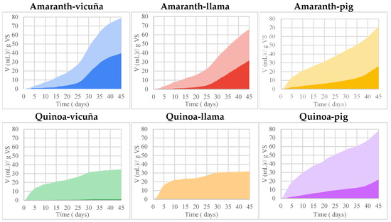
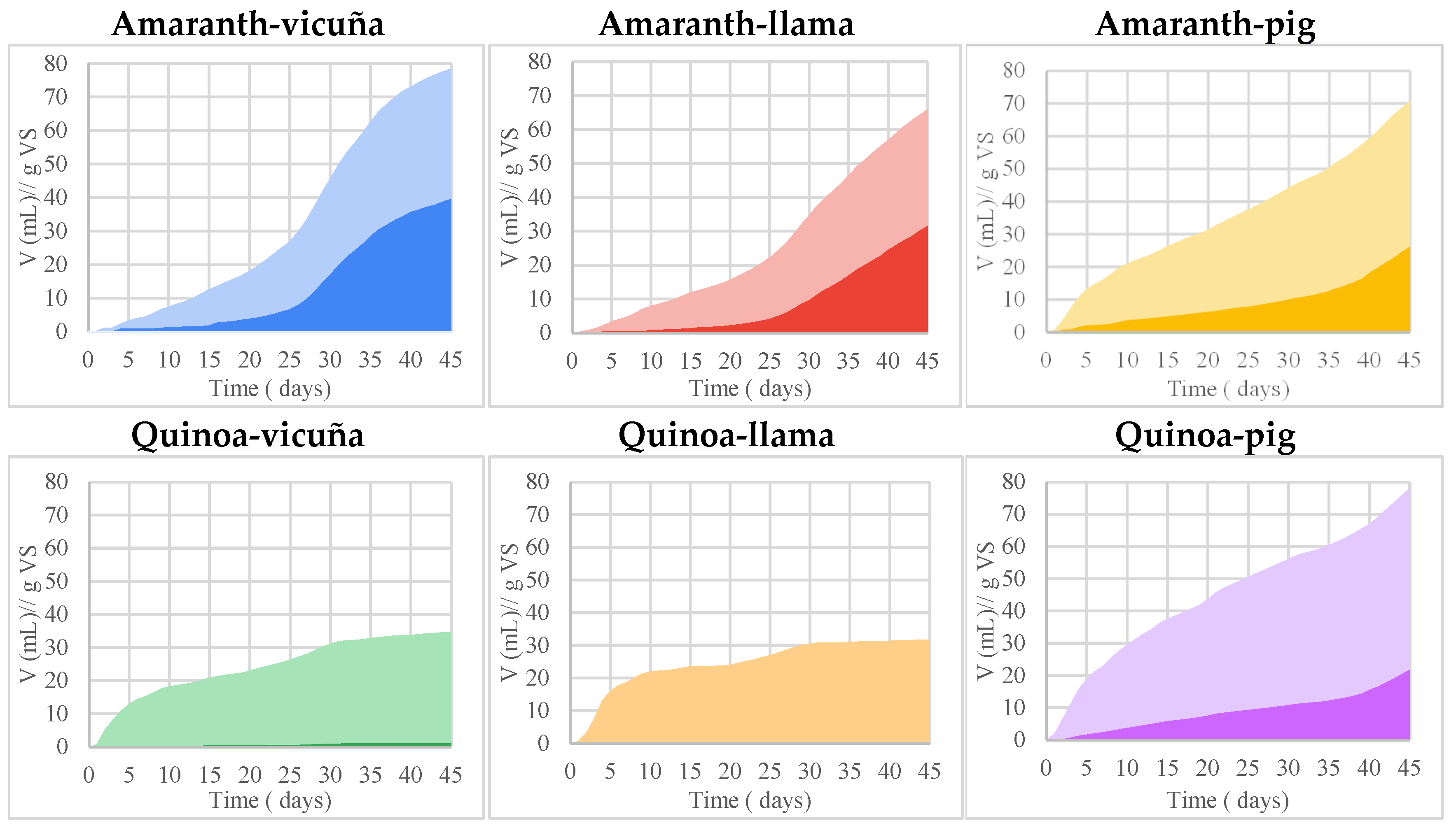
Figure 1 shows the daily evolution of cumulative biogas and CH₄. Each curve represents the mean of three independent replicates (n = 3). The dispersion of the final cumulative yield is presented as mean ± SD in Table 4.

Figure 1. Daily evolution of cumulative biogas and methane volume for each treatment. Curves represent the mean of n = 3 independent replicates. Variability in the final cumulative value is reported as mean ± SD in Table 4; treatment comparisons were evaluated using Tukey’s HSD test at α = 0.05. Source: prepared by the authors.

Table 4. Final cumulative biogas and CH₄ production. Values = mean ± SD (n = 3). Different letters within a column indicate significant differences (Tukey HSD, α = 0.05).

Treatment	Biogas Volume (mL/g VS)	Methane Volume (mL CH4/g VS)	CH4 Percentage in Biogas
Amaranth-vicuña	77.29 ± 5.63 a	36.20 ± 7.29 cd	46.84%
Amaranth-llama	64.62 ± 3.62 a	31.78 ± 3.62 cd	49.18%
Amaranth-pig	69.63 ± 0.89 a	26.02 ± 0.41 c	37.37%
Quinoa-vicuña	33.21 ± 1.17 b	1.04 ± 0.25 e	3.12%
Quinoa-llama	30.53 ± 0.84 b	0.24 ± 0.03 e	0.80%
Quinoa-pig	76.82 ± 9.21 a	21.90 ± 5.56 cd	28.51%

Note: Different letters indicate significant differences (p < 0.05, Tukey test).

Table 4 summarizes the final cumulative biogas and CH₄ yields and the significant differences among treatments determined by ANOVA and Tukey’s HSD test.

3.3. Kinetic Fitting to Traditional Models

Table 5 presents the parameters of the adapted Monod model (μ_max and K_s^ap) for each replicate and their mean values. The Quinoa-vicuña and Quinoa-llama treatments were excluded from this fit because their CH₄ production was virtually zero. R² coefficients are included as goodness-of-fit indicators.

Table 5. Parameters of the product-referenced adapted Monod model (μ_max and K_s^ap). Different letters indicate significant differences among treatments (Tukey HSD, α = 0.05).

	Replicate	μmax (Day−1)	R2 (μmax)	Mean μmax (Day−1)	Ksap (mL CH4/g VS)	R2 (Ksap)	Mean Ksap (mL CH4/g VS)
Amaranth -vicuña	1	0.04 *	0.9927	0.18 ± 0.01 a	0.92 *	0.9959 †	7.11 ± 1.18 a
	2	0.18	0.9937		6.27	0.9930
	3	0.17	0.9909		7.94	0.9850
Amaranth -llama	1	0.12	0.9466	0.11 ± 0.02 b	4.01	0.8277	2.88 ± 1.00 b
	2	0.12	0.9894		2.51	0.8068 †
	3	0.08	0.9761		2.12	0.8809 †
Amaranth -pig	1	0.08	0.9955	0.08 ± 0.00 bc	1.38	0.7183 †	1.75 ± 0.52 bc
	2	0.08	0.9956		2.02 *	0.4962 †
	3	0.07	0.9955		2.11	0.9094 †
Quinoa -pig	1	0.03	0.9549	0.05 ± 0.02 c	0.35	0.9777 †	0.37 ± 0.02 c
	2	0.04	0.9704		0.39	0.8394 †
	3	0.06	0.9473		2.70 *	0.7184 †

Note: Different letters indicate significant differences (p < 0.05, Tukey test) in each of the two analyses. The asterisk (*) indicates that the marked replicate was far from the mean or had a low correlation coefficient and was excluded. The dagger (†) indicates that K_s^ap in the marked replicates was calculated from the last four points of the exponential phase because stationary-phase data were not available.

The exponential-model parameters from Equation (14), including $Y_{P/S}·X_0,\mathsf{\mu }max$, and $t_{lag}$, are shown in Table 6 together with R² and RMSE.

Table 6. Exponential-model parameters (Equation (14)) obtained by nonlinear regression using Solver.

Treatment		${\mathit{Y}}_{\mathit{P}/\mathit{S}}$·X0 (mL CH4/g VS)		μmax (Day−1)		t_lag (Days)		R2	RMSE
Amaranth-vicuña	1 *	20.23 *	29.06 ± 2.19	0.04 *	0.16 ± 0.01	37.22 *	34.40 ± 3.11	0.9736	1.22
	2	27.51		0.16		36.59		0.9945	0.44
	3	30.61		0.17		32.20		0.9931	0.55
Amaranth-llama	1 *	40.77 *	31.66 ± 0.62	0.16 *	0.10 ± 0.00	37.37 *	44.61 ± 0.18	0.9949	0.28
	2	31.22		0.10		44.74		0.9888	0.96
	3	32.10		0.09		44.48		0.9798	1.46
Amaranth-pig	1	27.13	26.41 ± 0.70	0.06	0.06 ± 0.00	46.47	45.97 ± 0.96	0.9865	0.76
	2	26.37		0.06		46.58		0.9844	0.79
	3	25.72		0.07		44.86		0.9922	0.61
Quinoa-pig	1	17.32	20.33 ± 3.87	0.04	0.05 ± 0.01	45.32	44.66 ± 0.71	0.9400	1.13
	2	18.97		0.04		44.75		0.9498	1.14
	3	24.71		0.06		43.90		0.9720	1.17

For each parameter, the value for each replicate and the treatment mean ± SD are presented. An asterisk (*) identifies replicates excluded from the mean according to the criterion indicated in the text. This table is descriptive; no additional inferential test was applied to the model parameters.

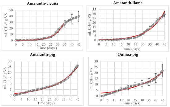
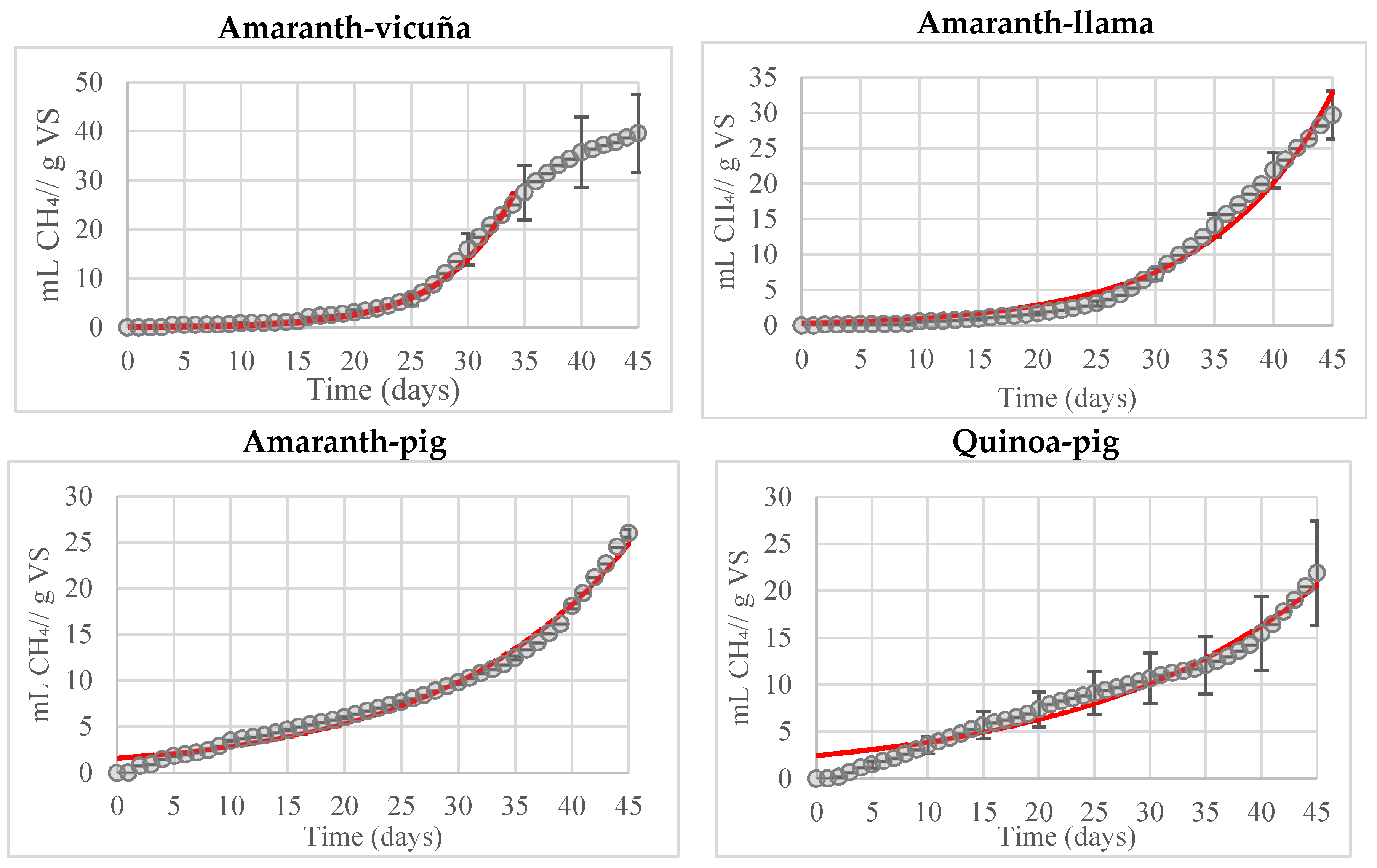
Figure 2 compares the mean experimental cumulative CH₄ curves with the curves calculated using the exponential model in Equation (14). The corresponding R² and RMSE metrics are presented in Table 6.

Figure 2. Comparison between experimental cumulative CH₄ production (mean of n = 3 replicates) and the exponential-model prediction for each treatment. R² and RMSE are shown in Table 6; no inferential significance level applies to these fit metrics. Source: prepared by the authors.

3.4. Prediction of Biogas Production Using Neural Networks

Table 7 summarizes the training characteristics and performance metrics of the ANNs evaluated to predict CH₄ production from the physicochemical characterization of the raw materials.

Table 7. Characteristics, architecture, and evaluation metrics of the ANNs trained to predict CH₄ production.

Network Number	Day	Number of Days	Inputs	Treatments	Data Type	Number of Layers	Neurons in Layer 1	Neurons in Layer 2	Neurons in Layer 3	Training R2	Validation R2	Test R2	Overall R2	Validation MSE	Final Epoch
1	Output	9	3 replicates	All	%	2	10	9	-	0.922	0.988	0.993	0.929	2.138	0
2						3	10	6	9	0.909	0.948	0.944	0.922	5.113	0
3						3	10	10	9	0.937	0.997	0.932	0.928	0.422	0
4	Output	9	Means	All	%	2	10	9	-	0.786	0.824	0.999	0.850	-	-
5						3	10	6	9	0.837	0.173	0.930	0.713	-	-
6						3	10	10	9	0.673	0.213	0.867	0.735	-	-
7	Output	9	3 replicates	Without Qui-Vic and Qui-Lla	%	2	10	9	-	0.681	0.835	0.904	0.726	-	-
8						3	15	10	9	0.810	0.776	0.829	0.783	-	-
9						3	10	10	9	0.899	0.992	0.967	0.918	-	-
10	Output	5	3 replicates	All	%	2	10	5	-	0.953	0.963	0.890	0.942	-	-
11						3	10	10	5	0.970	0.953	0.865	0.928	-	-
12						3	10	6	5	0.972	0.907	0.987	0.941	-	-
13	Output	5	Means	All	%	2	10	5	-	0.741	0.940	1.000	0.771	-	-
14						3	10	10	5	0.998	1.000	0.995	0.997	0.000	0
15						3	10	6	5	0.944	0.992	0.992	0.949	2.907	0
16	Output	9	Means	All	g/g VS	2	10	9	-	0.999	0.043	0.979	0.965	-	-
17						3	10	10	9	0.726	1.000	0.996	0.816	-	-
18						3	15	10	9	0.897	0.260	0.947	0.919	-	-
19	Output	9	3 replicates	All	g/g VS	2	10	9	-	0.953	0.977	0.981	0.927	-	-
20						3	10	10	9	0.537	0.393	0.885	0.545	-	-
21						3	15	10	9	0.960	0.867	0.981	0.933	-	-
22	Output	5	Means	All	g/g VS	2	10	5	-	0.901	0.950	1.000	0.929	-	-
23						3	10	10	5	0.772	1.000	1.000	0.810	-	-
24						3	10	5	5	0.259	0.010	1.000	0.472	-	-
25	Output	5	3 replicates	All	g/g VS	2	10	5	-	0.946	0.994	0.921	0.945	0.651	5
26						3	10	10	5	0.938	0.996	0.982	0.940	0.543	0
27						3	10	5	5	0.642	0.470	0.692	0.604	-	-
28	Input	9	Means	All	%	2	10	1	-	0.768	0.402	0.728	0.699	108.767	4
29						3	20	10	1	1.000	0.999	0.995	0.998	0.667	7
30						3	10	10	1	0.110	0.083	0.153	0.099	65.600	0
31	Input	9	Means	All	g/g VS	2	10	1	-	0.997	1.000	0.999	0.998	0.148	0
32						3	10	10	1	0.217	0.228	0.126	0.202	78.122	0
33						3	10	5	1	0.799	0.518	0.988	0.805	32.196	0
34	Input	5	Means	All	%	2	10	1	-	1.000	0.993	0.725	0.989	1.012	6
35						3	10	10	1	0.023	0.237	0.368	0.042	405.193	0
36						3	10	5	1	0.995	0.997	0.997	0.995	0.042	0
37	Input	5	Means	All	g/g VS	2	10	1	-	0.989	0.997	0.998	0.990	0.083	0
38						3	10	10	1	0.989	0.999	0.997	0.990	0.652	0
39						3	10	5	1	0.998	0.948	0.992	0.956	9.638	12
40	Output	3	3 replicates	All	%	2	10	3	-	0.958	0.999	0.968	0.965	0.227	6
41						3	10	5	3	0.667	0.316	0.467	0.574	132.281	0
42	Output	3	3 replicates	All	g/g VS	2	10	3	-	0.900	0.802	0.941	0.882	71.265	0
43						3	10	5	3	0.959	0.972	0.963	0.948	4.818	0

Day: indicates whether day was used as an input or output. Number of days: number of selected CH₄-production time points (9: days 5, 10, 15, 20, 25, 30, 35, 40, and 45; 5: days 5, 15, 25, 35, and 45; 3: days 5, 25, and 45). Inputs: indicates whether the three replicates were used individually or as their means. Treatments: indicates whether all treatments were included or low-production treatments were excluded. Data type: percentage on a dry basis or g/g VS. Training, validation, test, and overall R²: squares of the correlation coefficients provided by MATLAB. Validation MSE: mean squared error of the validation set. Epoch: iteration with the lowest validation MSE. These metrics are descriptive performance measures and are not associated with statistical significance tests.

After evaluating all configurations, Networks 25, 29, 34, 36, and 40 were preselected because they showed R² > 0.97 and validation curves without evident deterioration after the minimum MSE. Nevertheless, given the limited amount of data, these criteria were considered only as an initial screening step and not as sufficient evidence of generalization.

Of the five preselected networks, Network 40 was discarded because it generated predictions at only three times (days 5, 25, and 45), which was insufficient to represent the complete curve. Networks 25 and 34 were discarded because they showed R² < 0.99. Networks 29 and 36 were retained as final candidates: both used day as an input, the means of the three replicates, variables expressed as dry-basis percentages, and two hidden layers. Their main difference was the number of time points considered: nine for Network 29 and five for Network 36.Five additional architectures (Networks 44–48) were generated from Networks 29 and 36, retaining the input criteria while varying the number of neurons in the hidden layers. Their metrics are summarized in Table 8 together with the parent networks.

Table 8. Architecture and evaluation metrics of the optimized networks (Networks 44–48) derived from candidates 29 and 36. R² and MSE are performance metrics; no inferential significance tests were applied.

Network Number	Parent Network	Neuronas Capa 1	Neuronas Capa 2	Neuronas Capa 3	Training R2	Validation R2	Test R2	Overall R2	Validation MSE	Final Epoch
29	29	20	10	1	1.000	0.999	0.995	0.998	0.667	7
44		15	10	1	1.000	0.997	0.999	0.998	0.415	10
45		15	5	1	0.999	0.995	0.976	0.998	0.775	16
36	36	10	5	1	0.995	0.997	0.997	0.995	0.042	0
46		8	5	1	0.991	0.999	0.989	0.990	0.991	3
47		5	5	1	0.016	0.291	0.166	0.055	-	-
48		10	3	1	0.860	0.995	0.823	0.890	1.071	1

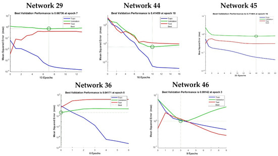
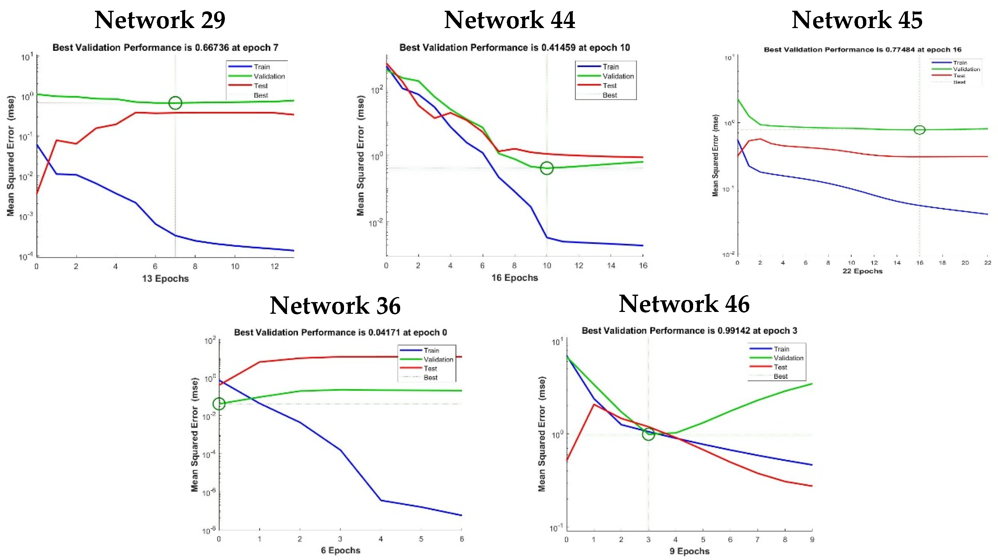
Among the Network 29 variants, Networks 44 and 45 achieved high R² values, but Network 44 had the lowest validation MSE and more stable error evolution. Among the variants derived from Network 36, Network 46 was the only one with acceptable performance; Networks 47 and 48 showed clearly lower R² values. Figure 3 presents the validation curves of the retained candidates.

Figure 3. Evolution of MSE during training, validation, and testing of the candidate ANNs in MATLAB. The curves are used to identify the validation minimum and possible signs of overtraining. MSE and R² are performance metrics, not inferential significance tests.

Network 44 was selected among the Network 29 variants because it combined the lowest validation MSE with stable curves and intermediate complexity. Between Networks 36 and 46, Network 46 was prioritized because Network 36 reached its validation minimum at epoch 0, a behavior that provides little information for assessing learning. Thus, Networks 44 and 46 were the finalists.

Network 44 was selected from the two finalist architectures. This network predicts cumulative CH₄ at nine time points (days 5–45) and yielded training R² = 1.000, validation R² = 0.997, test R² = 0.999, overall R² = 0.998, and validation MSE = 0.415. These values reflect a high internal fit but should be interpreted together with the cross-validation analysis and the small size of the dataset.

Network 44 uses 13 inputs: day and 12 variables derived from proximate, elemental, and structural characterization. The means of the three replicates for each treatment were used. Its architecture is 13-15-10-1, with two hidden layers of 15 and 10 neurons and one output neuron, and tansig activation in the hidden layers. Weights and biases are shown in Table 9.

Table 9. Weights and biases of the layers of Network 44. Descriptive table; no inferential significance tests were applied.

LAYER 1
		Inputs																																				Layer 1 Bias
		total g VS		Inoculum g TS			% Ash		% CF			% C			% H			% O				% N			% S		% Lignin			% Cellulose			% Hemicellulose			Day
Neurons in layer 1	N 1-1	−0.096		0.911			0.424		−0.130			−1.806			0.029			0.426				0.301			−1.240		1.614			−0.462			−1.022			−0.607		−3.095
	N 1-2	−0.830		0.706			−0.974		−0.077			0.534			−0.353			0.623				−1.034			0.496		−0.135			0.174			0.082			−0.109		1.749
	N 1-3	1.084		0.044			−0.205		−0.725			0.283			0.455			0.535				0.689			0.518		−0.113			−0.648			−0.668			−1.436		−1.661
	N 1-4	1.669		−0.527			−0.185		−0.483			1.354			0.744			−0.034				1.418			−0.925		0.923			−0.068			−0.184			1.823		−0.517
	N 1-5	−1.298		0.197			−0.828		1.076			0.336			−1.666			1.101				−0.921			0.838		−0.466			−0.186			−0.455			−1.354		−0.049
	N 1-6	0.217		−0.789			0.614		−0.985			0.369			−0.052			0.651				−0.593			1.165		−1.143			1.757			0.327			0.220		0.571
	N 1-7	0.537		0.746			1.465		−1.330			−0.477			0.296			−0.426				−0.035			−0.957		0.610			0.315			−0.882			−0.689		−0.642
	N 1-8	−0.230		−0.216			0.024		−0.926			0.409			0.361			0.498				0.557			−0.423		−0.696			0.929			−0.185			0.631		−0.201
	N 1-9	−0.180		1.401			0.912		0.231			−0.138			−1.714			0.906				−0.463			0.147		−0.562			0.842			0.083			2.150		0.779
	N 1-10	0.917		−0.959			−1.166		0.757			1.236			1.489			−0.357				0.516			0.109		1.163			−0.663			−1.811			−1.973		−0.261
	N 1-11	0.339		0.712			−0.260		−0.594			0.484			0.122			−0.090				−0.696			−0.052		0.604			0.728			−0.038			−3.534		0.598
	N 1-12	−0.164		−0.342			0.137		1.606			−0.808			−0.814			1.691				−0.464			0.456		0.208			−0.430			0.750			0.310		0.382
	N 1-13	−0.523		0.620			0.269		−0.288			−0.130			0.151			−1.084				0.880			−0.319		−0.336			−0.651			−0.621			2.221		−1.090
	N 1-14	−0.215		0.491			−0.408		−0.095			0.799			0.030			−0.484				0.512			−0.488		−0.356			−0.670			−0.505			0.827		−1.540
	N 1-15	−0.253		0.468			1.046		−1.145			−0.394			0.618			−0.362				0.424			−0.974		−0.313			0.743			0.206			1.100		1.816
LAYER 2
		Neurons in Layer 1																																				Layer 2 Bias
		N 1-1	N 1-2		N 1-3			N 1-4			N 1-5		N 1-6			N 1-7			N 1-8		N 1-9		N 1-10			N 1-11			N 1-12			N 1-13		N 1-14			N 1-15
Neurons in layer 2	N 2-1	−0.135	0.101		−0.204			0.097			−0.199		−1.334			0.771			−0.139		−0.941		0.762			0.881			−0.233			−0.742		1.217			0.500	2.074
	N 2-2	−0.530	0.718		−0.367			−0.598			0.368		0.515			−0.158			0.261		−0.233		−0.519			0.390			0.794			−0.300		0.385			−0.289	1.419
	N 2-3	0.231	0.134		1.414			−0.622			−0.118		−0.752			−0.369			−1.197		−1.718		−0.508			−0.480			−1.194			−0.330		−0.413			−0.002	−0.856
	N 2-4	−0.298	−0.732		0.282			0.781			0.524		−0.056			−0.309			−0.759		−0.185		0.869			0.497			−0.216			0.208		−0.209			0.071	0.210
	N 2-5	0.799	0.597		0.189			−1.620			1.210		−0.896			0.155			−0.195		0.347		−1.086			−1.087			−0.484			−0.986		0.720			1.260	−0.099
	N 2-6	0.654	−0.060		1947			0.885			0.811		−0.443			0.023			−0.039		−1.695		0.721			−0.052			−1.402			0.391		−0.704			0.171	−0.219
	N 2-7	−0.677	1.511		−1.643			−0.075			1.210		0.456			−0.184			−0.589		0.243		0.807			1.150			0.370			−1.039		−1.393			0.888	1.616
	N 2-8	0.635	0.315		−0.049			−1.195			0.102		0.652			0.296			−0.791		−0.485		0.446			0.420			0.394			−0.492		0.462			−0.234	0.367
	N 2-9	−0.241	−0.252		−1.137			−1.392			−0.479		1.606			−0.010			0.519		1.293		−0.710			0.643			2.152			0.831		−0.024			0.992	2.157
	N 2-10	0.345	−0.180		0.478			1.164			−0.237		0.816			−0.068			−0.151		0.092		0.297			0.346			−1.045			0.520		−0.010			0.308	−1.844
LAYER 3
			Neurons in Layer 2																																			Layer 3 Bias
			N 2-1			N 2-2				N 2-3				N 2-4			N 2-5			N 2-6				N 2-7				N 2-8			N 2-9				N 2-10
mL CH4/g VS			−0.811			−0.450				−0.630				−0.861			0.763			1.110				0.346				−1.435			−0.550				−0.065			−0.618

Ten-times repeated five-fold cross-validation produced an out-of-fold R² of 0.985 ± 0.007 and an RMSE of 1.21 ± 0.28 mL CH₄/g VS. The stability of these metrics supports the interpolation capability of the architecture within the sampled domain. However, the 54 patterns arise from only six substrate combinations and the network contains 381 trainable parameters; therefore, generalization to raw-material mixtures not represented in training is not considered demonstrated.

4. Discussion

4.1. Substrate Characterization

Analyses of the raw materials showed general similarities between the two lignocellulosic residues and among the three manures, although with differences relevant to biodegradability. VS represents the potentially degradable organic fraction and, together with TS, was used to determine the amount of substrate added to each digester [43]. Because of compositional differences, treatments with pig manure required a greater wet mass to provide the same VS fraction as treatments with llama or vicuña manure.

In the elemental analysis, the carbon-to-nitrogen (C/N) ratio is particularly relevant to AD. Values close to 20–30 have been proposed as a favorable range for balancing carbon and nitrogen availability for the microbial community [44]. Amaranth had a clearly higher C/N ratio than quinoa; therefore, combining it with manures having lower C/N ratios may help balance the mixture during ACD.

Structural analysis showed that quinoa contained more lignin and less cellulose than amaranth. Lignin limits enzymatic accessibility to the carbohydrate fraction and can make hydrolysis the rate-limiting step when no chemical or biological pretreatment is applied [45]. Li et al. [46] observed a positive relationship between cellulose content and methane production. Accordingly, the combination of higher cellulose and lower lignin in amaranth is consistent with its better performance as a co-substrate.

4.2. Biogas and Methane Production Among Treatments

Figure 1 and Table 4 show that Quinoa-vicuña and Quinoa-llama were the treatments with the lowest methanogenic activity: they produced 33.21 ± 1.17 and 30.53 ± 0.84 mL biogas/g VS, but only 1.04 ± 0.25 and 0.24 ± 0.03 mL CH₄/g VS, respectively. The gas fraction was therefore dominated by CO₂. These values are much lower than those reported by Meneses-Quelal et al. [37] for similar Andean mixtures and by Álvarez and Lidén [47] for co-digestion of quinoa stalks, indicating that the low methanogenesis observed cannot be attributed solely to the botanical identity of the residue.

The quinoa treatments showed an especially low CH₄ fraction when combined with vicuña and llama manure, while CO₂-rich biogas continued to be produced. This pattern is compatible with activity in the stages preceding methanogenesis together with a limited methanogenic response, but it does not by itself identify the responsible mechanism. pH, VFAs, alkalinity, and ammonia were not monitored during the experiment; therefore, acidification, VFA accumulation, ammonia inhibition, insufficient inoculum activity, or the presence of inhibitory compounds must be considered alternative hypotheses rather than demonstrated causes [48]. A possible role of quinoa saponins cannot be inferred from these data either. In fact, methane production from quinoa stalks has been demonstrated in previous studies using Andean manures [37,47], so the presence of quinoa alone does not constitute evidence of inhibition.

Amaranth-vicuña and Amaranth-llama showed profiles close to sigmoidal kinetics. Amaranth-vicuña achieved the highest CH₄ production (36.20 ± 7.29 mL CH₄/g VS), whereas Amaranth-llama reached 31.78 ± 3.62 mL CH₄/g VS and the highest methane fraction in the biogas (49.18%). Although these were the most favorable treatments in the experiment, their yields remained below those reported by Meneses-Quelal et al. [37] for co-digestion of amaranth with camelid manures.

Overall, CH₄ yields were low, but direct comparison with ranges of 150–500 mL CH₄/g VS should be made with caution. Many values of that magnitude correspond to BMP tests or digestion under controlled mesophilic conditions. For example, Meneses-Quelal et al. [37] studied related Andean mixtures at 37 °C, whereas Álvarez and Lidén [47] worked with quinoa stalks and manures at 25 °C. The present experiment was conducted without agitation or pretreatment and at an average laboratory temperature of approximately 18 °C to approximate a low-cost rural system. Specific studies in the Andes have shown that anaerobic digestion of camelid manure is feasible at high altitude and low temperature, although kinetics and productivity are strongly temperature-dependent [49,50,51,52,53]. Therefore, the low values observed demonstrate the yield achieved under these suboptimal conditions but, by themselves, do not constitute evidence of severe inhibition [54].

4.3. Kinetic Fitting to Traditional Models

The estimation of μ_max showed high linear fits for most replicates (R² > 0.99), indicating a well-defined exponential phase. Amaranth-vicuña had the highest mean μ_max (0.18 ± 0.01 d⁻¹), whereas Quinoa-pig had the lowest (0.05 ± 0.02 d⁻¹), consistent with their final CH₄ yields. These results support the use of μ_max as a comparative descriptor of the apparent process rate under the studied conditions.

Published specific rates depend strongly on substrate, reactor type, and the model used. Zinatizadeh et al. [55] obtained μ_max values of 0.207 and 0.304 d⁻¹ in continuous reactors treating palm-oil effluent. In batch systems, Phayungphan et al. [56] reported values < 0.12 d⁻¹ and Abu-Reesh [57] values around 0.07 d⁻¹. Thongnan et al. [58] obtained values close to 0.2 d⁻¹ for co-digestion of pig manure and food waste, although using a dual-substrate model. In this context, the values obtained in the present study fall within the range reported for anaerobic systems with different characteristics, and the comparison should therefore be regarded as indicative.

K_s^ap also differed among treatments (ANOVA, α = 0.05). Amaranth-vicuña had the highest mean value (7.11 ± 1.18 mL CH₄/g VS), followed by Amaranth-llama (2.88 ± 1.00), Amaranth-pig (1.75 ± 0.52), and Quinoa-pig (0.37 ± 0.02 mL CH₄/g VS).

The linearization used for K_s^ap generally yielded R² values above 0.8; replicates showing poorer behavior were identified and excluded according to the criterion described in Table 5. The weakest fit corresponded to Amaranth-pig. Because only a small number of points were used in some fits, these R² values should be interpreted as descriptive indicators rather than as independent validation of the model.

In the conventional Monod model, K_s is an affinity constant referred to a defined substrate concentration. K_s^ap has a different interpretation: it summarizes the relationship between the apparent process rate and the CH₄ generation rate. Its values are therefore useful for comparing treatments within this experiment, but they should not be interpreted as intrinsic constants or numerically compared with K_s values obtained from direct substrate measurements. This distinction is an explicit limitation of the proposed adaptation.

The choice of a reduced model therefore reflects an identifiability problem rather than an assumption that anaerobic digestion can be fully described by a single algebraic equation. A mechanistic differential model should represent, at a minimum, substrate consumption, biomass growth and decay, and product formation; in a real co-digestion system, it should also incorporate several substrate fractions and microbial groups. Without independent time series for these state variables, increasing the number of equations would have increased formal complexity without providing robustly identifiable parameters. The scope of the present approach is deliberately more limited: to compare the apparent rate and response of treatments subjected to the same protocol.

The effect of the estimation method should also be considered. The logarithmic transformation used for μ_max and the reciprocal transformation used for K_s^ap modify the residual distribution relative to a direct nonlinear fit and may affect the numerical value of the parameters, especially with few points or low CH₄ rates. This limitation does not invalidate the internal comparison, which used an identical procedure for all replicates, but it prevents the parameters from being interpreted as unique, method-independent estimates. With denser datasets including S(t), X(t), and intermediates, it would be preferable to compare these estimates with direct nonlinear regression and multivariable differential models.

The effective lag times estimated with the exponential model were long (approximately 34.4–46.0 days). However, these values are fitting parameters and are not equivalent to an observed phase of 34–46 days without biological activity. Figure 1 shows progressive biogas production during the experiment, and for several treatments the CH₄ curve did not reach a clear plateau; under these conditions, the $t_{lag}$ parameter may shift toward the end of the experimental interval. Therefore, a high $t_{lag}$ should not be interpreted directly as evidence of inoculum death. It does indicate a slow methanogenic response and warrants caution in interpretation. Because pH, VFAs, alkalinity, ammonia, and specific microbial activity were not measured over time, the experiment cannot discriminate among inoculum adaptation, hydrolysis limitation, transient acidification, or other inhibition mechanisms. These explanations are now presented only as plausible hypotheses and not as demonstrated causal relationships.

The exponential model adequately reproduced the growth phase of the treatments, with R² generally > 0.98 except for Quinoa-pig. Additional comparison with commonly used models showed that the modified logistic model achieved R²/RMSE values of 0.9972/0.734, 0.9989/0.334, and 0.9866/0.769 for Amaranth-vicuña, Amaranth-llama, and Amaranth-pig, respectively; the modified Gompertz model yielded 0.9923/1.229, 0.9974/0.507, and 0.9818/0.899. For Quinoa-pig, Gompertz performed slightly better (R² = 0.9672; RMSE = 1.001) than the logistic model (R² = 0.9611; RMSE = 1.089). The first-order model generally showed a poorer fit (R² = 0.7038–0.9620). These results confirm that sigmoidal functions describe curves approaching a plateau with high accuracy, whereas the adapted Monod formulation has a different purpose: obtaining apparent kinetic parameters with a comparative interpretation from product data [41,42,59,60].

4.4. Prediction of Biogas Production Using Neural Networks

ANN results are comparable to or better than those reported in several biogas-prediction studies, although direct comparisons depend on the size and heterogeneity of each dataset. Rego et al. [61] reported R² values up to 0.77 and Chong et al. [20] R² = 0.978, whereas Mougari et al. [62], using a substantially larger database, achieved R² > 0.999 and RMSE < 0.01. This contrast emphasizes that R² alone is insufficient to demonstrate generalization.

In Network 44, 381 trainable parameters are fitted to 54 patterns derived from six substrate combinations, so the structural risk of overfitting is high. The training-validation-test split and early stopping reduce this risk, and repeated cross-validation maintained high performance (R² = 0.985 ± 0.007; RMSE = 1.21 ± 0.28 mL CH₄/g VS). Nevertheless, the folds share treatments at different times, so the result mainly demonstrates temporal interpolation within compositions already represented. External validation with new substrates, or group-based validation leaving complete treatments out of training, will be necessary before the ANN can be used as a general design tool.

Other studies have used ANNs to predict AD performance by incorporating operating variables such as temperature, pH, VFAs, VS, and organic loading [63], and even genomic information from digesters [64]. Models have also been developed to predict H₂S in order to anticipate toxicity and corrosion problems [17]. Overall, the most common outputs are indicators of productivity, process stability, and organic-matter removal [23,65].

ANNs therefore show potential for reproducing the temporal evolution of CH₄ within the experimental domain, but Network 44 is not presented as a universal predictor. Repeated cross-validation provides evidence of internal stability, whereas extrapolation to new raw materials requires independent external validation. Synthetic data augmentation was not applied because, with only six original biological combinations, generating artificial observations would not add independent experimental information and could create an unjustified impression of generalization. Future expansion should rely primarily on new substrate combinations, operating conditions, and independent experimental campaigns.

4.5. Experimental Limitations and Scope

The main limitation for mechanistic interpretation is the absence of temporal monitoring of pH, VFAs, alkalinity, and ammonia. Such information would have allowed better discrimination among acidogenic instability, methanogen inhibition, and hydrolysis limitations. The absence of these variables does not change the measured gas volumes and compositions or the comparisons performed under a common protocol, but it prevents biochemical causality from being assigned to the low yields and slow response of some treatments.

Temperature was not recorded continuously either. A mean value of 18 °C was used for gas normalization, so thermal uncertainty mainly affects interpretation of biological rates. Altitude, by contrast, was incorporated into volumetric quantification through the measured local atmospheric pressure and correction to 25 °C and 1 atm. The feasibility of anaerobic digesters under high-altitude, low-temperature Andean conditions has been documented previously [49,50,51].

A complete carbon and nitrogen balance and microbial-community analysis were not performed. Both approaches would provide valuable information on conversion pathways, nutrient retention, and microbiological causes of the observed response, but they represent additional mechanistic characterization and are not prerequisites for the empirical comparison of specific gas production among treatments performed in this study.

Finally, the absence of chemical or enzymatic pretreatment was deliberate: the aim was to evaluate residues subjected to minimal conditioning compatible with low-cost rural digesters. Evaluating pretreatments is a logical continuation of the study, particularly for quinoa and other recalcitrant lignocellulosic materials, but introducing this factor into the present design would have added an experimental variable different from the original objective.

Similarly, the reduced kinetic formulation and its linearizations were choices constrained by the resolution of the dataset. The absence of substrate and biomass time series prevents identifiable calibration of a complete differential system; consequently, the constants obtained should be considered apparent parameters dependent on the experimental domain and the fitting procedure.

5. Conclusions

The quantitative results identified amaranth as the most favorable co-substrate. Amaranth-vicuña and Amaranth-llama reached 77.29 ± 5.63 and 64.62 ± 3.62 mL biogas/g VS and 36.20 ± 7.29 and 31.78 ± 3.62 mL CH₄/g VS, respectively. In contrast, Quinoa-vicuña and Quinoa-llama produced only 1.04 ± 0.25 and 0.24 ± 0.03 mL CH₄/g VS. The higher production with amaranth is consistent with its higher cellulose content (40.48% d.b.) and lower lignin content (9.93% d.b.) compared with quinoa (17.36% and 13.28% d.b., respectively).

In the kinetic analysis, Amaranth-vicuña showed the highest μ_max (0.18 ± 0.01 d⁻¹) and K_s^ap (7.11 ± 1.18 mL CH₄/g VS). The Monod adaptation provides apparent parameters useful for comparing treatments when a single residual substrate concentration is unavailable, but K_s^ap is not an intrinsic affinity constant. Additional fits showed that the modified logistic and Gompertz models achieved R² values of up to 0.9989 and 0.9974, respectively, outperforming the first-order model for several treatments.

High $t_{lag}$ values should be interpreted as effective fitting parameters rather than as direct evidence of 34–46 days of complete inoculum inactivity. The absence of time series for pH, VFAs, alkalinity, ammonia, and the microbial community prevents a single cause from being assigned to the slow response. Likewise, the yields obtained correspond to a low-cost system without agitation and operated at room temperature; therefore, they are not standardized BMP values and, by themselves, cannot be used to diagnose severe inhibition.

Network 44 (13-15-10-1) achieved overall R² = 0.998, validation R² = 0.997, test R² = 0.999, and validation MSE = 0.415. Repeated cross-validation yielded R² = 0.985 ± 0.007 and RMSE = 1.21 ± 0.28 mL CH₄/g VS. These results support good interpolation capability within the experimental domain, but the small number of substrate combinations and the high parameter-to-pattern ratio prevent a claim of general external robustness.

Consequently, the main contribution of the study is the combination of an apparent kinetic descriptor with an ANN capable of reproducing the temporal curve within the experimental space investigated. In its current form, the ANN is a proof of concept for interpolation. Any eventual capacity to reduce experimental workload can only be supported after external validation with new raw-material combinations and independent operating conditions; no extrapolation capability is attributed to the model presented here.

From an applied perspective, the results support the use of local agricultural by-products in low-cost digesters, but they also show that co-substrate selection, inoculum quality, and validation of the predictive model are critical. The conclusions are therefore restricted to the conditions and substrates evaluated in this study.

References

- Mella, C. Ecuador Suffers Power Outages of up to 14 Hours amid a Severe Energy Crisis; EL PAÍS América: Ciudad de México, México, 2024. [Google Scholar]
- Ministry of Agriculture and Livestock. Agricultural Statistics of Bolívar Province; Ministry of Agriculture and Livestock: Quito, Ecuador, 2023. [Google Scholar]
- Quijije Briones, V.M.; Ramos Rodríguez, M.P.; Villavicencio Valdez, D.G.; Manrique Toala, T.O. Diagnóstico Del Uso Del Fuego En Actividades Agrícolas En El Sitio Estancia Vieja, Cantón Portoviejo, Manabí, Ecuador. Cienc. Tecnol. 2025, 18, 48–63. [Google Scholar] [CrossRef]
- Eastern Research Group, Inc.; Tetra Tech. Resource Assessment for Livestock and Agro-Industrial Wastes—Ecuador; Global Methane Initiative: Washington, DC, USA, 2010. [Google Scholar]
- Nikolausz, M.; Kretzschmar, J. Anaerobic Digestion in the 21st Century. Bioengineering 2020, 7, 157. [Google Scholar] [CrossRef] [PubMed]
- Kapoor, R.; Ghosh, P.; Kumar, M.; Sengupta, S.; Gupta, A.; Kumar, S.S.; Vijay, V.; Kumar, V.; Kumar Vijay, V.; Pant, D. Valorization of Agricultural Waste for Biogas Based Circular Economy in India: A Research Outlook. Bioresour. Technol. 2020, 304, 123036. [Google Scholar] [CrossRef] [PubMed]
- Rocha-Meneses, L.; Zannerni, R.; Inayat, A.; Abdallah, M.; Shanableh, A.; Ghenai, C.; Kamil, M.; Kikas, T. Current Progress in Anaerobic Digestion Reactors and Parameters Optimization. Biomass Convers. Biorefin. 2025, 15, 29573–29596. [Google Scholar] [CrossRef]
- Gaibor-Chávez, J.; Niño-Ruiz, Z.; Meneses-Quelal, O. Advances in Biogas Production in Ecuador: A Research Perspective. In Proceedings of the Optimization of Solid Biomass Extraction Processes for Energy Use; IBEROMASA-CYTED: Valladolid, Spain, 2021; pp. 221–242. [Google Scholar]
- Marti-Herrero, J.; Cuji, P.; Ramírez, V.; Rodríguez, L.; Domínguez, D.L.; Cipriano, J. Towards a Sustainable Biodigester Sector in Ecuador: Inputs for a Biodigester Component of the PNBE; Climate Technology Centre & Network: Quito, Ecuador, 2019. [Google Scholar]
- Abatzoglou, N.; Boivin, S. A Review of Biogas Purification Processes. Biofuels Bioprod. Biorefining 2009, 3, 42–71. [Google Scholar] [CrossRef]
- Skiadas, I.V.; Lyberatos, G. Modeling of Anaerobic Digestion—A Review. Glob. NEST J. 1999, 1, 63–76. [Google Scholar]
- Velázquez-Martí, B.; Meneses-Quelal, O.W.; Gaibor-Chavez, J.; Niño-Ruiz, Z. Review of Mathematical Models for the Anaerobic Digestion Process. In Anaerobic Digestion; IntechOpen: London, UK, 2019. [Google Scholar]
- Kegl, T.; Torres Jiménez, E.; Kegl, B.; Kovač Kralj, A.; Kegl, M. Modeling and Optimization of Anaerobic Digestion Technology: Current Status and Future Outlook. Prog. Energy Combust. Sci. 2025, 106, 101199. [Google Scholar] [CrossRef]
- Batstone, D.J.; Keller, J.; Angelidaki, I.; Kalyuzhnyi, S.V.; Pavlostathis, S.G.; Rozzi, A.; Sanders, W.T.M.; Siegrist, H.; Vavilin, V.A. The IWA Anaerobic Digestion Model No 1 (ADM1). Water Sci. Technol. 2002, 45, 65–73. [Google Scholar] [CrossRef]
- Donoso-Bravo, A.; Mailier, J.; Martin, C.; Rodríguez, J.; Aceves-Lara, C.A.; Wouwer, A. Vande Model Selection, Identification and Validation in Anaerobic Digestion: A Review. Water Res. 2011, 45, 5347–5364. [Google Scholar] [CrossRef] [PubMed]
- Kunatsa, T. The Role of Artificial Intelligence in Greening Biogas Operations. In Innovations in the Global Biogas Industry; Elsevier: Amsterdam, The Netherlands, 2025; pp. 361–397. [Google Scholar]
- Levstek, T.; Lakota, M. The Use of Artificial Neural Networks for Compounds Prediction in Biogas from Anaerobic Digestion—A Review. Agricultura 2010, 7, 15–22. [Google Scholar]
- Wu, Y.; Feng, J. Development and Application of Artificial Neural Network. Wirel. Pers. Commun. 2018, 102, 1645–1656. [Google Scholar] [CrossRef]
- Serna, M.E.; Acevedo, M.E.; Serna, A.A. Integration of Properties of Virtual Reality, Artificial Neural Networks, and Artificial Intelligence in the Automation of Software Tests: A Review. J. Softw. Evol. Process 2019, 31, e2159. [Google Scholar] [CrossRef]
- Chong, D.J.S.; Chan, Y.J.; Arumugasamy, S.K.; Yazdi, S.K.; Lim, J.W. Optimisation and Performance Evaluation of Response Surface Methodology (RSM), Artificial Neural Network (ANN) and Adaptive Neuro-Fuzzy Inference System (ANFIS) in the Prediction of Biogas Production from Palm Oil Mill Effluent (POME). Energy 2023, 266, 126449. [Google Scholar] [CrossRef]
- Liu, Y.; Starzyk, J.A.; Zhu, Z. Optimized Approximation Algorithm in Neural Networks Without Overfitting. IEEE Trans. Neural Netw. 2008, 19, 983–995. [Google Scholar] [CrossRef] [PubMed]
- Owamah, H.I.; Izinyon, O.C. Development of Simple-to-Apply Biogas Kinetic Models for the Co-Digestion of Food Waste and Maize Husk. Bioresour. Technol. 2015, 194, 83–90. [Google Scholar] [CrossRef] [PubMed]
- Andrade Cruz, I.; Chuenchart, W.; Long, F.; Surendra, K.C.; Renata Santos Andrade, L.; Bilal, M.; Liu, H.; Tavares Figueiredo, R.; Khanal, S.K.; Fernando Romanholo Ferreira, L. Application of Machine Learning in Anaerobic Digestion: Perspectives and Challenges. Bioresour. Technol. 2022, 345, 126433. [Google Scholar] [CrossRef] [PubMed]
- Khatri, N.; Khatri, K.K. Artificial Intelligence for Modeling and Optimization of the Biogas Production. In Artificial Intelligence for Renewable Energy Systems; Wiley: Hoboken, NJ, USA, 2022; pp. 93–113. [Google Scholar]
- Instituto Nacional de Meteorología e Hidrología (INAMHI). Meteorological Yearbook; Nos. 53-2013; Instituto Nacional de Meteorología e Hidrología (INAMHI): Quito, Ecuador, 2017. [Google Scholar]
- American Public Health Association (APHA); American Water Works Association (AWWA); Water Environment Federation (WEF). 2540 SOLIDS. In Standard Methods for the Examination of Water and Wastewater, 24th ed.; American Public Health Association (APHA): Washington, DC, USA; American Water Works Association (AWWA): Denver, CO, USA; Water Environment Federation (WEF): Alexandria, VA, USA, 2022. [Google Scholar]
- ISO 18134-1:2022; Solid Biofuels—Determination of Moisture Content—Oven Dry Method—Part 1: Total Moisture—Reference Method. International Organization for Standardization (ISO): Geneva, Switzerland, 2022.
- ISO 18123:2023; Solid Biofuels—Determination of the Content of Volatile Matter. International Organization for Standardization (ISO): Geneva, Switzerland, 2023.
- ISO 18122:2022; Solid Biofuels—Determination of Ash Content. International Organization for Standardization (ISO): Geneva, Switzerland, 2022.
- Velázquez-Martí, B. Characterization of Solid Biomass. In Biomass Utilization for Energy Use, 2nd ed.; Chapter III; Reverté: Barcelona, Spain, 2018; pp. 631–662. [Google Scholar]
- ISO 16948:2015; Solid Biofuels—Determination of Total Content of Carbon, Hydrogen and Nitrogen. International Organization for Standardization (ISO): Geneva, Switzerland, 2015.
- ANKOM Technology. ANKOM2000 Fiber Analyzer Operator’s Manual; ANKOM Technology: Macedon, NY, USA, 2022. [Google Scholar]
- Van Soest, P.J.; Robertson, J.B.; Lewis, B.A. Methods for Dietary Fiber, Neutral Detergent Fiber, and Nonstarch Polysaccharides in Relation to Animal Nutrition. J. Dairy Sci. 1991, 74, 3583–3597. [Google Scholar] [CrossRef] [PubMed]
- Velázquez-Martí, B. Anaerobic Fermentation-Biogas. In Biomass Utilization for Energy Use, 2nd ed.; Chapter XIII; Reverté: Barcelona, Spain, 2018; pp. 631–662. [Google Scholar]
- Uddin, M.M.; Wright, M.M. Anaerobic Digestion Fundamentals, Challenges, and Technological Advances. Phys. Sci. Rev. 2023, 8, 2819–2837. [Google Scholar] [CrossRef]
- Holliger, C.; Alves, M.; Andrade, D.; Angelidaki, I.; Astals, S.; Baier, U.; Bougrier, C.; Buffière, P.; Carballa, M.; de Wilde, V.; et al. Towards a Standardization of Biomethane Potential Tests. Water Sci. Technol. 2016, 74, 2515–2522. [Google Scholar] [CrossRef] [PubMed]
- Meneses-Quelal, O.; Velázquez-Martí, B.; Gaibor-Chávez, J.; Niño-Ruiz, Z. Effect of the Co-digestion of Agricultural Lignocellulosic Residues with Manure from South American Camelids. Biofuels Bioprod. Biorefining 2021, 15, 525–544. [Google Scholar] [CrossRef]
- Monod, J. The Growth of Bacterial Cultures. Annu. Rev. Microbiol. 1949, 3, 371–394. [Google Scholar] [CrossRef]
- Hossain, S.M.; Das, M. Mathematical Modeling of Distillery Wastewater Biomethanation in Fluidized-Bed Bioreactor. Chem. Eng. Res. Bull. 2010, 14, 37–43. [Google Scholar] [CrossRef]
- Doran, P.M. Homogeneous Reactions. In Bioprocess Engineering Principles; Elsevier: Amsterdam, The Netherlands, 2013; pp. 599–703. [Google Scholar]
- Pramanik, S.K.; Suja, F.B.; Porhemmat, M.; Pramanik, B.K. Performance and Kinetic Model of a Single-Stage Anaerobic Digestion System Operated at Different Successive Operating Stages for the Treatment of Food Waste. Processes 2019, 7, 600. [Google Scholar] [CrossRef]
- Kafle, G.K.; Chen, L. Comparison on Batch Anaerobic Digestion of Five Different Livestock Manures and Prediction of Biochemical Methane Potential (BMP) Using Different Statistical Models. Waste Manag. 2016, 48, 492–502. [Google Scholar] [CrossRef] [PubMed]
- Zamri, M.F.M.A.; Hasmady, S.; Akhiar, A.; Ideris, F.; Shamsuddin, A.H.; Mofijur, M.; Fattah, I.M.R.; Mahlia, T.M.I. A Comprehensive Review on Anaerobic Digestion of Organic Fraction of Municipal Solid Waste. Renew. Sustain. Energy Rev. 2021, 137, 110637. [Google Scholar] [CrossRef]
- Dhull, P.; Kumar, S.; Yadav, N.; Lohchab, R.K. A Comprehensive Review on Anaerobic Digestion with Focus on Potential Feedstocks, Limitations Associated and Recent Advances for Biogas Production. Environ. Sci. Pollut. Res. 2024, 32, 19129–19164. [Google Scholar] [CrossRef] [PubMed]
- S, K.K.; Ibrahim, M.H.; Quaik, S.; Ismail, S.A. An Introduction to Anaerobic Digestion of Organic Wastes. In Prospects of Organic Waste Management and the Significance of Earthworms; Springer International Publishing: Cham, Switzerland, 2016; pp. 23–44. [Google Scholar]
- Li, Y.; Jin, Y.; Li, H.; Borrion, A.; Yu, Z.; Li, J. Kinetic Studies on Organic Degradation and Its Impacts on Improving Methane Production during Anaerobic Digestion of Food Waste. Appl. Energy 2018, 213, 136–147. [Google Scholar] [CrossRef]
- Alvarez, R.; Lidén, G. Anaerobic Co-Digestion of Aquatic Flora and Quinoa with Manures from Bolivian Altiplano. Waste Manag. 2008, 28, 1933–1940. [Google Scholar] [CrossRef] [PubMed]
- Meegoda, J.N.; Li, B.; Patel, K.; Wang, L.B. A Review of the Processes, Parameters, and Optimization of Anaerobic Digestion. Int. J. Environ. Res. Public Health 2018, 15, 2224. [Google Scholar] [CrossRef] [PubMed]
- Martí-Herrero, J.; Alvarez, R.; Cespedes, R.; Rojas, M.R.; Conde, V.; Aliaga, L.; Balboa, M.; Danov, S. Cow, Sheep and Llama Manure at Psychrophilic Anaerobic Co-Digestion with Low Cost Tubular Digesters in Cold Climate and High Altitude. Bioresour. Technol. 2015, 181, 238–246. [Google Scholar] [CrossRef] [PubMed]
- Alvarez, R.; Lidén, G. Low Temperature Anaerobic Digestion of Mixtures of Llama, Cow and Sheep Manure for Improved Methane Production. Biomass Bioenergy 2009, 33, 527–533. [Google Scholar] [CrossRef]
- Alvarez, R.; Villca, S.; Lidén, G. Biogas Production from Llama and Cow Manure at High Altitude. Biomass Bioenergy 2006, 30, 66–75. [Google Scholar] [CrossRef]
- Ali, S.A.S.T.A.A.T.R. Evaluating the Co-Digestion Effects on Chicken Manure and Rotten Potatoes in Batch Experiments. Int. J. Biosci. 2017, 10, 150–159. [Google Scholar] [CrossRef]
- Xie, S.; Lawlor, P.G.; Frost, J.P.; Hu, Z.; Zhan, X. Effect of Pig Manure to Grass Silage Ratio on Methane Production in Batch Anaerobic Co-Digestion of Concentrated Pig Manure and Grass Silage. Bioresour. Technol. 2011, 102, 5728–5733. [Google Scholar] [CrossRef] [PubMed]
- Zheng, Z.; Liu, J.; Yuan, X.; Wang, X.; Zhu, W.; Yang, F.; Cui, Z. Effect of Dairy Manure to Switchgrass Co-Digestion Ratio on Methane Production and the Bacterial Community in Batch Anaerobic Digestion. Appl. Energy 2015, 151, 249–257. [Google Scholar] [CrossRef]
- Zinatizadeh, A.A.L.; Mohamed, A.R.; Najafpour, G.D.; Hasnain Isa, M.; Nasrollahzadeh, H. Kinetic Evaluation of Palm Oil Mill Effluent Digestion in a High Rate Up-Flow Anaerobic Sludge Fixed Film Bioreactor. Process Biochem. 2006, 41, 1038–1046. [Google Scholar] [CrossRef]
- Phayungphan, K.; Rakmak, N.; Promraksa, A. Application of Monod Two-Substrate Kinetics with an Intermediate for Anaerobic Co-Digestion of Distillery Wastewater and Molasses/Glycerol Waste in Batch Experiments. Water Pract. Technol. 2020, 15, 1068–1082. [Google Scholar] [CrossRef]
- Abu-Reesh, I.M. Kinetics of Anaerobic Digestion of Labaneh Whey in a Batch Reactor. Afr. J. Biotechnol. 2014, 13, 1745–1755. [Google Scholar] [CrossRef]
- Thongnan, R.; Thongpan, H.; Rakmak, N.; Siripatana, C. Modeling of Anaerobic Co-Digestion of Pig Manure and Domestic Organic Waste. J. Teknol. 2016, 78, 117–124. [Google Scholar] [CrossRef]
- Li, W.; Khalid, H.; Zhu, Z.; Zhang, R.; Liu, G.; Chen, C.; Thorin, E. Methane Production through Anaerobic Digestion: Participation and Digestion Characteristics of Cellulose, Hemicellulose and Lignin. Appl. Energy 2018, 226, 1219–1228. [Google Scholar] [CrossRef]
- Romero-Güiza, M.S.; Vila, J.; Mata-Alvarez, J.; Chimenos, J.M.; Astals, S. The Role of Additives on Anaerobic Digestion: A Review. Renew. Sustain. Energy Rev. 2016, 58, 1486–1499. [Google Scholar] [CrossRef]
- Rego, A.; Leite, S.; Leite, B.; Grillo, A.V.; Santos, B.F. Artificial Neural Network Modelling for Biogas Production in Biodigesters. Chem. Eng. Trans. 2019, 74, 25–30. [Google Scholar] [CrossRef]
- Mougari, N.E.; Largeau, J.F.; Himrane, N.; Hachemi, M.; Tazerout, M. Application of Artificial Neural Network and Kinetic Modeling for the Prediction of Biogas and Methane Production in Anaerobic Digestion of Several Organic Wastes. Int. J. Green Energy 2021, 18, 1584–1596. [Google Scholar] [CrossRef]
- Flores-Asis, R.; Méndez-Contreras, J.M.; Juárez-Martínez, U.; Alvarado-Lassman, A.; Villanueva-Vásquez, D.; Aguilar-Lasserre, A.A. Use of Artificial Neuronal Networks for Prediction of the Control Parameters in the Process of Anaerobic Digestion with Thermal Pretreatment. J. Environ. Sci. Health Part A 2018, 53, 883–890. [Google Scholar] [CrossRef] [PubMed]
- Long, F.; Wang, L.; Cai, W.; Lesnik, K.; Liu, H. Predicting the Performance of Anaerobic Digestion Using Machine Learning Algorithms and Genomic Data. Water Res. 2021, 199, 117182. [Google Scholar] [CrossRef] [PubMed]
- Zahan, Z.; Othman, M.Z.; Muster, T.H. Anaerobic Digestion/Co-Digestion Kinetic Potentials of Different Agro-Industrial Wastes: A Comparative Batch Study for C/N Optimisation. Waste Manag. 2018, 71, 663–674. [Google Scholar] [CrossRef] [PubMed]
Disclaimer/Publisher’s Note: The statements, opinions and data contained in all publications are solely those of the individual author(s) and contributor(s) and not of MDPI and/or the editor(s). MDPI and/or the editor(s) disclaim responsibility for any injury to people or property resulting from any ideas, methods, instructions or products referred to in the content. |
© 2026 by the authors. Licensee MDPI, Basel, Switzerland. This article is an open access article distributed under the terms and conditions of the Creative Commons Attribution (CC BY) license.