Deep Projected Gradient Network to Accelerate Low-Carbon Economic Dispatch Considering Energy Storage

Abstract

Under the strategic goals of “peak carbon emissions and carbon neutrality”, traditional methods for solving economic dispatch problems involving carbon emission trading costs, wind power, and energy storage devices lack real-time performance and are difficult to support in real-time decision-making. This paper proposes an accelerated solution framework that expands the projection gradient descent method into a Deep Projected Gradient Network (D-PGNet). The network consists of K structured layers, each layer strictly embedding differentiable projection operations corresponding to physical constraints such as power balance, unit ramp-up, and energy storage timing dynamics. This paper systematically derived the projection closed-form solutions of each constraint set to the basic subset, designed an efficient differentiable projection layer based on Dykstra alternating projection, and analyzed the differentiability and convergence properties of the network. Multiple scenario tests have shown that the optimal gap of D-PGNet results is less than 1.08%, the carbon emission deviation is less than 0.2%, the solving speed is improved by more than 64 times at most, and the maximum violation of all physical constraints is below 1.3 × 10⁻⁵ p.u.

1. Introduction

Building a new type of power system with new energy as the main body is the key path for achieving carbon peak and carbon neutrality goals in the energy sector [1]. In 2021, the national carbon emission trading market was officially launched, and power generation enterprises, as the first batch to be included in the industry, have internalized their carbon emission costs as a core economic factor that must be considered for dispatch and operation [2,3,4]. At the same time, the penetration rate of volatile renewable energy such as wind power and photovoltaics continues to rise, and the large-scale configuration of energy storage systems has made the economic dispatch (ED) of the power system face unprecedented complexity: decision variables need to cover multiple time periods of thermal power output, new energy consumption, and energy storage charging and discharging, and constraints include strong time-related constraints such as unit ramp-up and energy storage state of charge (SOC) deep temporal coupling. The optimization problem scale increases linearly with the number of scheduling time periods and equipment, presenting high-dimensional, multi-constraint convex quadratic programming (QP) characteristics [5,6,7,8].

In traditional solving methods, although the interior-point method (such as the primal–dual interior-point method), sequential quadratic programming, or decomposition algorithms based on Lagrangian relaxation can obtain accurate optimal solutions, their computation time increases superlinearly with the size of variables, especially when repeated rolling optimization or scene analysis is required. The solution time in seconds to minutes has become a bottleneck for online applications [9,10,11]. For example, using commercial solvers CPLEX or Gurobi to solve ED problems involving hundreds of time periods and dozens of units typically takes several seconds, while distributed methods based on alternating direction multipliers (ADMMs), although parallelizable, still require tens to hundreds of iterations to converge, which makes it difficult to meet the demand for millisecond-level response in real-time scheduling.

In recent years, deep learning technology has been introduced into the field of power system optimization and scheduling due to its millisecond inference ability, forming a research hotspot of “data-driven scheduling”. A representative approach is to use deep neural networks to directly learn the mapping from load and new energy forecasting to schedule plans, and construct end-to-end black-box prediction models [12,13,14]. For example, reference [12] uses fully connected networks to predict the optimal power flow solution, reference [13] uses deep reinforcement learning for real-time economic scheduling, and reference [14] proposes graph neural networks for safety-constrained unit combinations. These works have achieved remarkable acceleration effects. However, such purely data-driven methods generally have two inherent flaws: Firstly, it is difficult to guarantee that the output decision will meet complex physical constraints, so post-processing corrections (such as power rebalancing or hill clipping) are often required, which can disrupt the optimality structure and result in uncontrollable and unquantifiable optimality losses. Secondly, the model relies on a large number of labeled training data generated by traditional solvers, and it is expensive to obtain labels, and the network is fitted purely from the perspective of data mapping, lacking explicit use of the mathematical structure of the optimization problem itself, which results in limited generalization capability—when the system topology, load mode or new energy penetration rate changes, the model performance may decline significantly.

Another type of more promising approach originates from the “Learning to Optimize” or “Algorithm Unfolding” paradigms [15,16,17]. Algorithm unfolding maps each iteration of an iterative optimization algorithm to a layer of a deep neural network and forms a structured network by unfolding a fixed number of iterations into a feedforward computation graph. The network parameters (such as step size and regularization coefficient) can be trained end-to-end, which allows for a very small number of layers (such as 5–10 layers) to approximate the exact solution. At the same time, the network structure directly inherits the convergence properties and physical significance of the original algorithm, combining efficiency and interpretability. This paradigm has achieved great success in sparse coding [18], compressive sensing [19], image restoration [20], and other fields, but its application in power system optimization scheduling is still in its infancy. A few pioneering works have used the interior-point method or ADMM expansion for optimal power flow calculation [21,22], but most of them have ignored carbon emission constraints and did not fully consider the temporal coupling complexity brought by energy storage.

Projected gradient descent (PGD) is a classic first-order algorithm for solving smooth optimization problems with convex constraints. Each iteration consists of a gradient descent step and a Euclidean projection step to the feasible domain, naturally ensuring the feasibility of the iteration points. Expanding PGD into a network, the projection layer is equivalent to pulling infeasible points back into the constraint manifold, thereby structurally eliminating constraint violations. However, efficient and differentiable projection implementation is the key to the success of this approach: precise and computationally efficient projection operators must be designed for the power balance, ramp-up, and energy storage dynamic constraints unique to power dispatch, and their differentiability must be ensured to support backpropagation training.

Based on the above motivation, this paper proposes a Projection Gradient Unfolding Network (D-PGNet) that integrates carbon emission costs and addresses the ED problem of wind storage systems. The main innovative points are as follows:

• Low-carbon scheduling modeling: Explicitly incorporating carbon emission trading costs into the ED objective function and synergistically modeling with energy storage temporal dynamics and wind curtailment penalties to form a standard convex QP provides a unified mathematical framework for low-carbon optimization.
• Physical constraint differentiable projection design: For the established model, the complex feasible domain is decomposed into the intersection of power balance hyperplane, ramp-rate polyhedron, energy storage dynamic subspace, and box set. The closed projection operator for each basic subset is systematically derived. Specifically, an analytical projection based on matrix inversion was derived for the energy storage timing equation, and an efficient and differentiable bidirectional scanning algorithm was developed for the ramp-rate constraint. The overall feasible region projection was achieved through the Dykstra alternating projection strategy to ensure that the output achieves high feasibility with residual violations below specified thresholds.
• Label-free self-supervised learning mechanism: The loss function directly adopts the original scheduling objective, and the network only needs scene data (load, wind power prediction) during the training process, without the need for traditional solvers to generate optimal scheduling labels, which greatly reduces the cost of data acquisition and enables the network to autonomously learn low-carbon output allocation guided by carbon price signals.

Table 1 compares the proposed D-PGNet with representative data-driven dispatch methods. Unlike pure black-box predictors, D-PGNet structurally embeds physical constraints via differentiable projections, eliminating the need for post-processing. Unlike OptNet, which differentiates through a QP solver, D-PGNet uses lightweight closed-form projection operators, enabling fast inference even on large-scale systems. To our knowledge, this is the first work to unfold projected gradient descent for an ED problem that simultaneously includes carbon trading, wind curtailment, and full time-coupled energy storage dynamics, all trained without optimal-solution labels. Beyond the summary, D-PGNet further offers three distinct advantages. First, the Dykstra alternating projection maintains solutions directly on the constraint manifold, avoiding the optimality loss associated with penalty-based corrections in DeepOPF. Second, the closed-form sub-projections yield linear complexity in generator count and time steps, contrasting with the cubic scaling of embedded QP solvers. Third, the self-supervised loss that directly minimizes dispatch costs, including carbon expenses, allows rapid adaptation to new carbon prices without re-labeling, obviating the large labeled datasets required by supervised unfolding approaches.

Table 1. Comparison of Representative Data-driven Methods.

Method	Constraint Handling	Storage Dynamics	Carbon Cost	Unsupervised Training
D-PGNet	Embedded projections	Yes (full SOC)	Yes	Yes
DeepOPF	Penalty/post-proc	No	No	No (needs labels)
OptNet	Differentiable QP	Possible	Possible	No
RL-based	Reward shaping	Partially	Partially	Yes (RL)

2. Materials and Methods

2.1. Low-Carbon Economic Dispatch Model

2.1.1. Objective Function

Consider a power system consisting of $N_g$ thermal power units, a centralized wind farm, and a battery storage power station, with a scheduling cycle of $T$ time periods and a unit time period length $\Delta t=1$. The decision variables include: the active output of thermal power unit $i$ during time period $t$, $P_{g,t}^i\left(i=1,\dots ,N_g\right)$; wind farm grid-connected power $P_{w,t}$; energy storage charging power $P_{ch,t}$ and discharge power $P_{dis,t}$; and the state of charge (SOC) of energy storage, denoted as $E_t$. The scheduling objective is to minimize the total operating cost (1) throughout the entire cycle, expressed as:

$$\min F={\displaystyle \sum _{t=1}^T}\left[{\displaystyle \sum _{i=1}^{N_g}}{C}_i\left(P_{g,t}^i\right)+C_{\mathrm{carbon},t}+C_{w,t}\right],$$

(1)

The definitions of each cost item are as follows:

•

Fuel cost: the classic quadratic model $C_i\left(P\right)=a_i{P}^2+b_{i}P+c_i$ is adopted, where $a_i$, $b_i$, and $c_i$ are the fuel cost coefficients of the i-th unit, reflecting the heat rate characteristics of the unit.

•

Carbon emission cost: $C_{\mathit{carbon},t}=c_{\mathit{carbon}}{\sum }_{i=1}^{N_g}{e}_i{P}_{g,t}$. Here, $e_i$ is the carbon emission intensity of unit $i$ (tCO₂/MWh), and $c_{\mathit{carbon}}$ is the carbon market trading price ($/tCO₂). This model directly linearly converts the carbon emissions of the unit into economic costs, equivalent to adding an additional term $c_{\mathit{carbon}}{e}_i$ to the marginal cost.

•

Wind curtailment penalty: $C_{w,t}=c_w\left(P_{w,t}^{\mathrm{fore}}-P_{w,t}\right)$, where $P_{w,t}^{\mathrm{fore}}$ is the maximum predicted wind power output for period $t$, and $c_w$ is the wind curtailment penalty factor ($/MWh).

The objective function is a quadratic convex function with a linear term. All cost coefficients are positive, which ensures the strong convexity of the objective function.

Although the objective function contains linear terms for wind power and energy storage variables, its Hessian with respect to the full decision vector $x$ is block-diagonal. The block corresponding to thermal generations $P_{g,t}^i$ is positive definite because all ai > 0. The remaining blocks for $P_w, P_{ch}, P_{dis}, E$ are zero. However, within the feasible region defined by the equality constraints (power balance and energy storage dynamics) and inequality bounds, the thermal block strict convexity propagates to guarantee uniqueness of the global minimum. This can be seen by eliminating $P_w, P_{ch}, P_{dis}$ via the linear equalities, which leaves a reduced QP in the thermal variables with a positive definite Hessian. Therefore, the solution of the economic dispatch problem (1) is unique.

2.1.2. Constraints

The scheduling plan must strictly meet the following operational constraints to ensure the safe and stable operation of the power system.

• System active power balance constraint (ignoring network loss)

At each time period $t$, the total power generation and load must be balanced (2):

$$\sum _{i=1}^{N_g}{P}_{g,t}^i+P_{w,t}+P_{dis,t}-P_{ch,t}=L_t,\hspace{1em}\hspace{1em}\forall t$$

(2)

Among them, $L_t$ is the load forecast value for period $t$.

2.

Upper and lower limit constraints on the output of thermal power units

The output of each unit is limited by its physical capacity (3):

$$P_{g,min}^i\le P_{g,t}^i\le P_{g,max}^i,\hspace{1em}\hspace{1em}\forall i,\forall t$$

(3)

3.

Unit ramp-rate constraint

The output variation during adjacent time periods is limited by the ramp-rate limits of the unit (4):

$$-\Delta P_{g,\mathrm{down}}^i\le P_{g,t}^i-P_{g,t-1}^i\le \Delta P_{g,\mathrm{up}}^i,\hspace{1em}\hspace{1em}\forall i,\forall t$$

(4)

At $t=1$, $P_{g,0}^i$ is the known output at the end of the previous scheduling cycle, which is given as the initial condition. The ramp-rate constraint couples the output sequences of each unit, which is one of the main sources of time dimension complexity in ED.

4.

Wind power output constraint

The actual grid-connected power of wind power cannot be negative and does not exceed the available wind energy at that moment (5):

$$0\le P_{w,t}\le P_{w,t}^{\mathit{fore}},\hspace{1em}\hspace{1em}\forall t$$

(5)

5.

Operational constraints of energy storage system

The energy storage system must meet the requirements of energy storage dynamics, capacity limitations, power limitations, and cycle sustainability.

•

SOC recursive Equation (6):

$$E_t=E_{t-1}+{\eta }_{ch}{P}_{ch,t}-{\displaystyle \frac{1}{{\eta }_{dis}}}{P}_{dis,t},\hspace{1em}\hspace{1em}\forall t$$

(6)

Among them, ${{\eta }_{ch},\eta }_{dis}\in \left(\mathrm{0,1}\right]$ are the charging and discharging efficiencies, respectively. This equation accurately describes the energy loss during the charging and discharging process.

•

SOC safety range (7):

$$E_{min}\le E_t\le E_{max},\hspace{1em}\hspace{1em}\forall t$$

(7)

Avoid deep discharge or overcharging to extend battery life.

•

Charge and discharge power limit (8):

$$0\le P_{ch,t}\le P_{ch,max},\hspace{1em}\hspace{1em}0\le P_{dis,t}\le P_{dis,max},\hspace{1em}\hspace{1em}\forall t$$

(8)

And the complementary constraint $P_{ch,t}\cdot P_{dis,t}=0$ indicates that charging and discharging cannot be carried out simultaneously during the same time period. In continuous optimization, this complementary constraint can be relaxed because simultaneous charging and discharging will result in unnecessary energy loss, which, naturally, does not hold in the optimal solution.

•

End-of-cycle energy balance (9):

$$E_T=E_0$$

(9)

Ensure that the energy storage SOC returns to the initial value $E_0$ after the scheduling cycle ends so that each scheduling day is independent and reproducible.

2.2. Deep Projected Gradient Network

2.2.1. Projection Gradient Method

Projection Gradient Method (PGD) is a simple and effective first-order iterative algorithm for solving problem (1). Given the initial point ${\mathit{x}}^{\left(0\right)}$, the $k$th iteration consists of two steps.

• Gradient descent step (10):

  $${\mathit{z}}^{\left(k\right)}={\mathit{x}}^{\left(k\right)}-{\mathit{\alpha }}_k\nabla \mathit{f}\left({\mathit{x}}^{\left(k\right)}\right)$$

  (10)

  where $\nabla f\left({\mathit{x}}^{\left(\mathit{k}\right)}\right)=\mathit{Q}{\mathit{x}}^{\left(\mathit{k}\right)}+\mathit{p}$.
• Feasible region projection step (11):

  $${\mathit{x}}^{\left(k+1\right)}={\mathsf{\Pi }}_{\mathcal{X}}\left({\mathit{z}}^{\left(k\right)}\right)=\mathit{arg}{\displaystyle \underset{\mathit{x}\in \mathcal{X}}{\mathit{min}}}{|\mathit{x}-{\mathit{z}}^{\left(k\right)}|}^2$$

  (11)

The projection operator ${\mathsf{\Pi }}_{\mathcal{X}}$ ensures that each iteration update is within the feasible domain. When the objective function satisfies the smoothness condition and the constraint set is a closed convex set, taking a fixed step size $\mathsf{\alpha }\in (0,2/L_f)$ (where $L_f$ is the gradient Lipschitz constant), PGD can linearly converge to the optimal solution ${\mathit{x}}^{\ast }$ [23]. However, traditional PGD often requires dozens to hundreds of iterations to achieve high accuracy, and each iteration requires solving the casting shadow problem, without reducing the total computational complexity.

The core idea of algorithm unfolding is to fix the first $K$ iterations of PGD as a feedforward computational graph, where the projection subproblem of each iteration is approximated by a customized and efficient algorithm, and the step size ${\alpha }_k$ and initial point generation method are allowed to learn from the data. In this way, the unfolded network only needs to perform $K$-step forward propagation to directly output high-quality solutions without repeating iterations, thus transforming a slow optimization solving process into an extremely fast neural network inference process.

2.2.2. D-PGNet

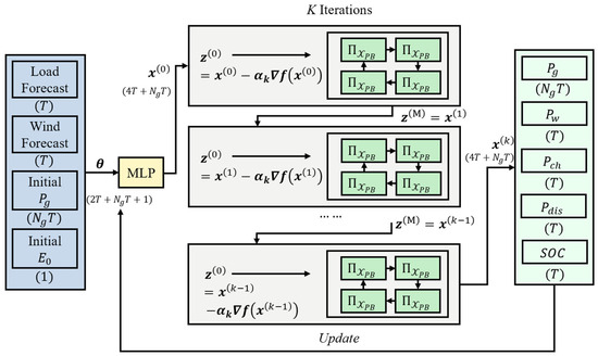
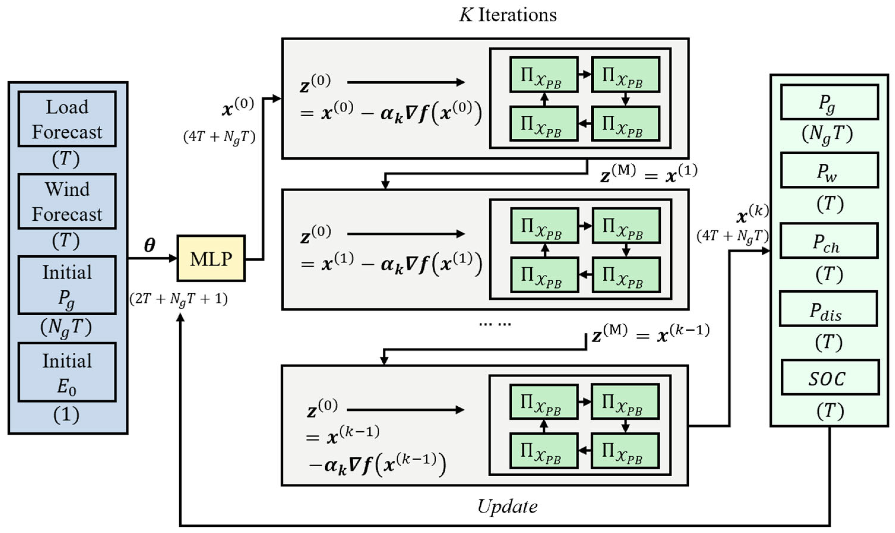
The overall architecture of D-PGNet is shown in Figure 1, and the training process is shown in Algorithm 1. The network input is the scene parameter vector $\mathit{\theta }$ (12), defined as:

$$\mathit{\theta }={\left[L_1,\dots ,L_T,P_{w,1}^{\mathit{fore}},\dots ,P_{w,T}^{\mathit{fore}},P_{g,0}^1,\dots ,P_{g,T}^{N_g},E_0 \right]}^{\top }\in {\mathbb{R}}^{2T+N_{g}T+1}$$

(12)

Figure 1. D-PGNet Architecture.

It includes the load of each time period, wind power forecast, initial output of each thermal power plant, and initial SOC of energy storage. The network output is the scheduling decision ${\mathit{x}}^{\left(\mathit{K}\right)}$, which is the solution after $K$ layers are unfolded.

Unlike standard PGD, which starts from a fixed point, we introduce a learnable initial guessing network ${\mathrm{MLP}}_{\mathsf{\varphi }}$, whose input is $\mathit{\theta }$ and output is ${\mathit{x}}^{\left(0\right)}$ (13):

$${\mathit{x}}^{\left(0\right)}={\mathit{MLP}}_{\varphi }\left(\theta \right)$$

(13)

This MLP typically consists of two fully connected hidden layers. Through training, ‘MLP’ can provide an initial point for each scenario that is close to the feasible region and the optimal solution, significantly reducing the required number of expansion layers $K$.

Next, the network performs $K$-layer iteration (10) and (11).

Algorithm1. Training of D-PGNet

Input: Training dataset D with scenario parameters θ, steps K, Dykstra alternating projection cycles M, total training epochs I. Output: network parameters Θ, dispatch decision $x^{\left(k\right)}$

1. Randomly initialize Θ

2. For epoch = 1 to I do 3. For each batch of size D do

4.  $x^{\left(0\right)}={\mathit{MLP}}_{\varphi }\left(\theta \right)$

5.    For $\mathit{k}$ = 0 to K − 1 do 6.     ${\mathit{z}}^{\left(k\right)}={\mathit{x}}^{\left(k\right)}-{\mathit{\alpha }}_k\nabla \mathit{f}\left({\mathit{x}}^{\left(k\right)}\right)$

7.     For iter = 0 to M − 1 do 8.     ${\mathbf{z}}^{(k+1)}\leftarrow {\mathsf{\Pi }}_{{\mathcal{X}}_{PB}}\left({\mathbf{z}}^{\left(k\right)}+{\mathit{p}}_{PB}^{\left(k\right)}\right)$, ${\mathit{p}}_{PB}^{(k+1)}={\mathit{p}}_{PB}^{\left(k\right)}+{\mathbf{z}}^{\left(k\right)}-{\mathbf{z}}^{(k+1)}$ 9.     ${\mathbf{z}}^{(k+1)}\leftarrow {\mathsf{\Pi }}_{{\mathcal{X}}_{ramp}}\left({\mathbf{z}}^{\left(k\right)}+{\mathit{p}}_{ramp}^{\left(k\right)}\right)$, ${\mathit{p}}_{ramp}^{(k+1)}={\mathit{p}}_{ramp}^{\left(k\right)}+{\mathbf{z}}^{\left(k\right)}-{\mathbf{z}}^{(k+1)}$ 10.      ${\mathbf{z}}^{(k+1)}\leftarrow {\mathsf{\Pi }}_{{\mathcal{X}}_{ESS}}\left({\mathbf{z}}^{\left(k\right)}+{\mathit{p}}_{ESS}^{\left(k\right)}\right)$, ${\mathit{p}}_{ESS}^{(k+1)}={\mathit{p}}_{ESS}^{\left(k\right)}+{\mathbf{z}}^{\left(k\right)}-{\mathbf{z}}^{(k+1)}$ 11.      ${\mathbf{z}}^{(k+1)}\leftarrow {\mathsf{\Pi }}_{{\mathcal{X}}_{box}}\left({\mathbf{z}}^{\left(k\right)}+{\mathit{p}}_{box}^{\left(k\right)}\right)$, ${\mathit{p}}_{box}^{(k+1)}={\mathit{p}}_{box}^{\left(k\right)}+{\mathbf{z}}^{\left(k\right)}-{\mathbf{z}}^{(k+1)}$ 12.   End For 13.   ${\mathit{x}}^{\left(k+1\right)}={\mathbf{z}}^{\left(M\right)}$ 14.  End For 15.  ${\mathit{x}}_b^{\left(k\right)}={\mathit{x}}^{\left(k\right)}$ 16.  $\mathcal{L}\left(\mathsf{\Theta }\right)={\displaystyle \frac{1}{B}}{\sum }_{b=1}^B\left(f\left(x_b^{\left(K\right)}\right)+w\left(v\left(x_b^{\left(K\right)}\right)\right)\right)$ 17.  Update Θ 18. End For 19. End For 20. Return Θ, $x^{\left(k\right)}$

2.2.3. Design of Feasible Domain Decomposition and Differentiable Projection Operator

Directly calculating the precise projection of polyhedron X requires solving a medium-sized QP, which can be achieved through differentiable optimization layers such as OptNet [24] but has a high computational burden and requires additional solver support. We note that X can be represented as the intersection of several simpler sets of basic constraints (14):

$$\mathcal{X}={\mathcal{X}}_{PB}\cap {\mathcal{X}}_{ramp}\cap {\mathcal{X}}_{ESS}\cap {\mathcal{X}}_{box}$$

(14)

To compute the projection of a point $\mathbf{z}$ onto the intersection of the convex sets $\mathcal{X}$, we adopt the Dykstra alternating projection algorithm [25]. The classical alternating projection method simply cycles through the subsets as (15):

$$\mathbf{z}\leftarrow {\mathsf{\Pi }}_{{\mathcal{X}}_{PB}}(\mathbf{z})\to {\mathsf{\Pi }}_{{\mathcal{X}}_{ramp}}(\mathbf{z})\to {\mathsf{\Pi }}_{{\mathcal{X}}_{ESS}}(\mathbf{z})\to {\mathsf{\Pi }}_{{\mathcal{X}}_{box}}(\mathbf{z})$$

(15)

But it does not generally converge to the exact Euclidean projection onto the intersection. Dykstra’s algorithm overcomes this limitation by introducing auxiliary correction variables ${\mathit{p}}_m$ for each subset, and it is converged [26]. Starting from ${\mathbf{z}}^{\left(0\right)}=\mathbf{z}$ and ${\mathit{p}}_m^{\left(0\right)}=0$, the update for the m-th sub-projection becomes (16):

$${\mathbf{z}}^{(k+1)}={\mathsf{\Pi }}_{{\mathcal{X}}_m}({\mathbf{z}}^{\left(k\right)}+{\mathit{p}}_m^{\left(k\right)}), {\mathit{p}}_m^{(k+1)}={\mathit{p}}_m^{\left(k\right)}+{\mathbf{z}}^{\left(k\right)}-{\mathbf{z}}^{(k+1)}$$

(16)

After a full cycle through all four subsets, the sequence is guaranteed to converge to the true metric projection onto $\mathcal{X}$, and when all constituent sets are convex, the convergence rate is linear. In practice, we perform M = 20 complete Dykstra cycles, which reduces constraint violations to negligible levels (<1.3 × 10⁻⁵), as numerically validated in Section 3.3.

The closed-form solutions for each sub-projection are derived one by one below.

• Projection onto the power balance hyperplane ${\mathcal{X}}_{\mathit{P}\mathit{B}}$

For the constraint (2) in a single time period $\mathrm{t}$, let the relevant decision variables be $y_1,\dots ,y_{N_g}$ (thermal power), $y_{N_g+1}$ (wind power), $y_{N_g+2}$ (discharge), and $y_{N_g+3}$ (charging). The equation can be written as ${\mathit{c}}^{\top }\mathit{y}=L_t$, where $\mathit{c}={\left[1,\dots , 1, 1, 1,-1\right]}^{\top }$. The Euclidean projection formula from the current point $\tilde{\mathit{y}}$ to the hyperplane (17) is:

$${\mathit{y}}^{\mathit{proj}}=\tilde{\mathit{y}}-{\displaystyle \frac{{\mathit{c}}^{\mathbf{\top }}\tilde{\mathit{y}}-L_t}{|\mathit{c}{|}^2}}\mathit{c}$$

(17)

Due to ${\left|\mathbf{c}\right|}^2=N_g+3$, and the adjustment amount (18):

$$\Delta ={\displaystyle \frac{L_t-\left({\sum }_{i=1}^{N_g}\widetilde{{\mathrm{y}}_i}+\stackrel{~}{{\mathrm{y}}_{{\mathrm{N}}_{\mathrm{g}}+1}}+\stackrel{~}{{\mathrm{y}}_{{\mathrm{N}}_{\mathrm{g}}+2}}-\stackrel{~}{{\mathrm{y}}_{{\mathrm{N}}_{\mathrm{g}}+3}}\right)}{N_g+3}}$$

(18)

Therefore, the projection is:

•

For variables with a coefficient of +1 (thermal power, wind power, discharge), add Δ to each variable;

•

For variables with a coefficient of −1 (charging), subtract Δ.

This operation can be achieved through tensor broadcasting, with minimal computational complexity and differentiability everywhere.

2.

Projection onto the ramp-rate-constrained polyhedron ${\mathcal{X}}_{\mathit{r}\mathit{a}\mathit{m}\mathit{p}}$

The ramp-rate constraint only involves the time series of a single unit, without cross-unit coupling. For unit $i$, its output vector ${\mathit{p}}^{\mathit{i}}={\left[{\mathrm{P}}_{\mathrm{g},1}^{\mathrm{i}},\dots ,{\mathrm{P}}_{\mathrm{g},\mathrm{T}}^{\mathrm{i}}\right]}^{\top }$ must satisfy (19):

$$\left|p_t^i-p_{t-1}^i\right|\le {\Delta }_i,\hspace{1em}\hspace{1em}\forall \mathrm{t}=1,\dots ,\mathrm{T}$$

(19)

where ${\mathrm{p}}_0^{\mathrm{i}}={\mathrm{P}}_{\mathrm{g},0}^{\mathrm{i}}$, it is known that ${\Delta }_i$ can take the smaller of the upper and lower limits of ramp rate. Projection onto this constraint set is equivalent to solving a least squares problem with linear inequality constraints, and there is a well-known iterative algorithm called forward and backward scanning (also known as “projection onto a total variation sphere” [27]). The specific steps are as follows:

•

Forward scan ($\mathrm{t}=1\to \mathrm{T}-1$): If ${\mathrm{p}}_{\mathrm{t}+1}-{\mathrm{p}}_{\mathrm{t}}>{\Delta }_{\mathrm{i}}$, then let ${\mathrm{p}}_{\mathrm{t}+1}={\mathrm{p}}_{\mathrm{t}}+{\Delta }_{\mathrm{i}}$; if ${\mathrm{p}}_{\mathrm{t}+1}-{\mathrm{p}}_{\mathrm{t}}<-{\Delta }_{\mathrm{i}}$, then let ${\mathrm{p}}_{\mathrm{t}}={\mathrm{p}}_{\mathrm{t}+1}-{\Delta }_{\mathrm{i}}.$

•

Backward scan ($\mathrm{t}=\mathrm{T}\to 2$): If ${\mathrm{p}}_{\mathrm{t}}-{\mathrm{p}}_{\mathrm{t}-1}>{\Delta }_{\mathrm{i}}$, then let ${\mathrm{p}}_{\mathrm{t}}={\mathrm{p}}_{\mathrm{t}-1}+{\Delta }_{\mathrm{i}}$; if ${\mathrm{p}}_{\mathrm{t}}-{\mathrm{p}}_{\mathrm{t}-1}<-{\Delta }_{\mathrm{i}}$, then let ${\mathrm{p}}_{\mathrm{t}-1}={\mathrm{p}}_{\mathrm{t}}-{\Delta }_{\mathrm{i}}$.

Repeat the above forward and backward scanning 2–3 times to converge to accurate projection.

3.

Projection onto energy storage dynamic affine space ${\mathcal{X}}_{\mathit{E}\mathit{S}\mathit{S}}$

The most crucial constraints in energy storage are Equations (6) and (9). Order $\mathit{v}={\left[{\mathit{E}}^{\mathbf{\top }},{\mathit{P}}_{\mathrm{c}}^{\mathbf{\top }},{\mathit{P}}_{\mathit{dis}}^{\mathbf{\top }}\right]}^{\mathbf{\top }}\in {\mathbb{R}}^{3T}$; the equation can be written as $\mathit{M}\mathit{v}={\mathit{b}}_{\mathit{E}\mathit{S}\mathit{S}}$, where $\mathit{M}$ is defined as:

•

For $\mathrm{t}=1$: ${\mathit{M}}_{\mathrm{1,1}}=1,{\mathit{M}}_{1,\mathrm{T}+1}=-{\eta }_{\mathrm{ch}}, {\mathit{M}}_{\mathrm{1,2}\mathrm{T}+1}={\displaystyle \frac{1}{{\eta }_{\mathrm{dis}}}}, {RHS\mathit{b}}_1=E_0$.

•

For $\mathrm{t}=2,\dots ,\mathrm{T}$: ${\mathit{M}}_{\mathrm{t},\mathrm{t}-1}=-1,{\mathit{M}}_{\mathrm{t},\mathrm{T}+\mathrm{t}}=-{\eta }_{\mathrm{ch}}, {\mathit{M}}_{\mathrm{t},2\mathrm{T}+\mathrm{t}}={\displaystyle \frac{1}{{\eta }_{\mathrm{dis}}}}, {RHS\mathit{b}}_{\mathrm{t}}=0$.

•

Final state constraint: ${\mathit{M}}_{\mathrm{T}+1,\mathrm{T}}=1, {RHS\mathit{b}}_{\mathrm{T}+1}=E_0$

This is a linear system with $T$ equations. $\mathit{M}$ is a $\mathrm{T}\times 3\mathrm{T}$ sparse matrix. The projection Formula (20) to the affine space $\{\mathit{v}\mid \mathit{M}\mathit{v}=\mathit{b}\}$ is:

$${\mathit{v}}^{\mathit{po}}=\mathit{v}-{\mathit{M}}^{\mathbf{\top }}{\left(\mathit{M}{\mathit{M}}^{\mathbf{\top }}\right)}^{-1}\left(\mathit{M}\mathit{v}-\mathit{b}\right)$$

(20)

Due to $T=24$ and matrix $\mathit{M}{\mathit{M}}^{\mathbf{\top }}$ being 24 × 24, the inverse calculation is extremely small, which results in extremely high efficiency. The projected $\mathit{E}$ may not necessarily meet the capacity constraint, and subsequent ${\mathcal{X}}_{box}$ projections will handle it.

4.

Projection onto box constraint ${\mathcal{X}}_{\mathit{b}\mathit{o}\mathit{x}}$

This projection (21) is cropped element by element with upper and lower bounds:

$$x_i^{\mathrm{proj}}=\mathit{max}\left(l_i,\mathit{min}\left(x_i,u_i\right)\right)$$

(21)

Among them, $l_i,u_i$ are defined by the boundaries of the corresponding variables in equations. This operation is the commonly used clamp function, which is differentiable and hardware-accelerated.

2.2.4. Differentiability, Convergence, and Complexity Analysis

• Differentiability: The power balance projection (17) is an affine operation and, thus, differentiable everywhere. The ramp projection, though iterative, consists of elementwise clipping and comparison, which are piecewise linear and differentiable almost everywhere (except on a set of measure zero). The energy storage affine projection (19) is linear and, hence, differentiable. The box clamp (21) is also piecewise linear. Because the composition of piecewise differentiable functions remains differentiable almost everywhere, the overall projection layer supports gradient backpropagation in practice, as confirmed by our training.
• Convergence: The original projected gradient method with constant step size ${\mathit{\alpha }}_{\mathit{k}}\in (0,2/L_f)$ converges linearly to the optimum. By unfolding K iterations into a network, our D-PGNet can be viewed as a truncated optimization process. The learnable step sizes and initial point network allow the unfolded system to achieve a solution accuracy comparable to many more iterations of the standard algorithm, as demonstrated numerically.
• Computational complexity: Each Dykstra cycle involves four projections: power balance $\left(O\right(N_{g}T\left)\right)$, ramp rate $\left(O\right(N_{g}T)$ via bidirectional sweeping), energy storage affine update $(O\left(T^2\right)$ using a precomputed 25 × 2525 × 25 inverse), and box clamping $O\left(N_{g}T\right)$. Thus, one projection cycle costs $O\left(N_{g}T\right)$. With $K$ unfolded layers and $M$ projection cycles, the total inference complexity is $O\left(KM{N}_{g}T\right)$. By contrast, the interior-point method scales as $O{\left(N_{g}T\right)}^3$ per Newton step, which becomes prohibitive for large systems. This linear complexity underlies the >64× speedup observed relative to commercial solvers.

2.2.5. Loss Function

D-PGNet adopts a self-supervised training method: without any labels, the loss function is the objective function $f$ and regularization violation term $v$ of the original problem. For a batch of data containing $B$ scenes, the loss (22) is:

$$\mathcal{L}\left(\mathsf{\Theta }\right)={\displaystyle \frac{1}{B}}\sum _{b=1}^B\left(f\left(x_b^{\left(K\right)}\right)+w\left(v\left(x_b^{\left(K\right)}\right)\right)\right)$$

(22)

where $w$ is the weight of the regularization violation term. The network minimizes costs by adjusting the parameter $\mathsf{\Theta }$, essentially learning how to minimize operating costs for $K$-step unfolding, which is completely consistent with the fundamental goal of scheduling problems.

3. Results

3.1. Testing System and Parameter Settings

All experiments were conducted on a server with a 72-core Intel Xeon processor, 1007.5 GB RAM, and a single NVIDIA RTX A6000 GPU (48 GB memory). The software environment includes Python 3.9, PyTorch 2.6.0, CUDA 12.4, and CVXPY 1.4. The training of D-PGNet for 30 epochs on 4000 samples required approximately 800 s on average, with a batch size of 128.

To verify the effectiveness and adaptability of the proposed D-PGNet method in power systems of different scales, cases 6, 14, 39, 57, and 118 were selected as test cases over six independent runs with different random seeds, and custom parameters were defined. The main parameters for each system are shown in Table 2, and other system parameter settings are shown in Table A1. All systems are equipped with a centralized energy storage device, whose capacity and power limits are scaled according to the proportion of the total power generation capacity of the system. To eliminate the differences in numerical magnitudes between different systems, all power variables are standardized based on the total power generation capacity $S_{base}$ of the system, and energy variables are standardized based on the upper limit $E_{base}$ of energy storage capacity.

Table 2. System Parameters.

System	${\mathit{N}}_{\mathit{g}}$	∑Pmax (MW)	Energy Storage Capacity (MWh)	Wind Power Installed Capacity (MW)	Basic ${\mathit{c}}_{\mathbf{carbon}}$ ($/tCO2)
Case 6	3	280	200	100	30.0
Case 14	5	360	150	100	30.0
Case 39	10	1030	180	100	30.0
Case 57	7	740	180	100	30.0
Case 118	54	5400	180	150	30.0

The dataset is constructed from 24 h time series for load and wind power. The base load profile follows a sinusoidal shape with a mean of 0.5 per unit, reaching its peak of 0.65 at 12:00 noon and its minimum of 0.35 at midnight. The base wind profile evolves synchronously with the load, determined by the ratio of installed wind capacity to the system base power: its mean equals 0.4 times this ratio, and its variation amplitude equals 0.3 times this ratio. To represent forecast uncertainty, independent zero-mean Gaussian disturbances are added to both base profiles at each hour, with standard deviations of 0.03 p.u. for the load error and 0.02 p.u. for the wind error. A total of 5000 scenarios are generated via Monte Carlo sampling, of which 4000 are used for training, 500 for validation, and 500 for testing.

The hyperparameters of D-PGNet are uniformly set as follows: expansion step K = 5, projection layer iteration times 20, initial network hidden layer width 256, learning rate 10⁻⁵, cosine annealing scheduling. The constraint penalty weights in training loss are set in the order of power balance, unit output, energy storage charging and discharging power, SOC equation, and SOC boundary. The CVXPY benchmark prioritizes calling the Gurobi 9.5 solver (convergence tolerance of 10⁻⁸) and, if unavailable, reverts to OSQP high-precision mode.

3.2. Training Convergence

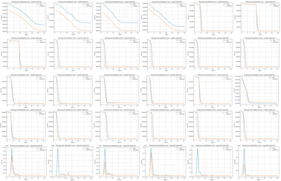
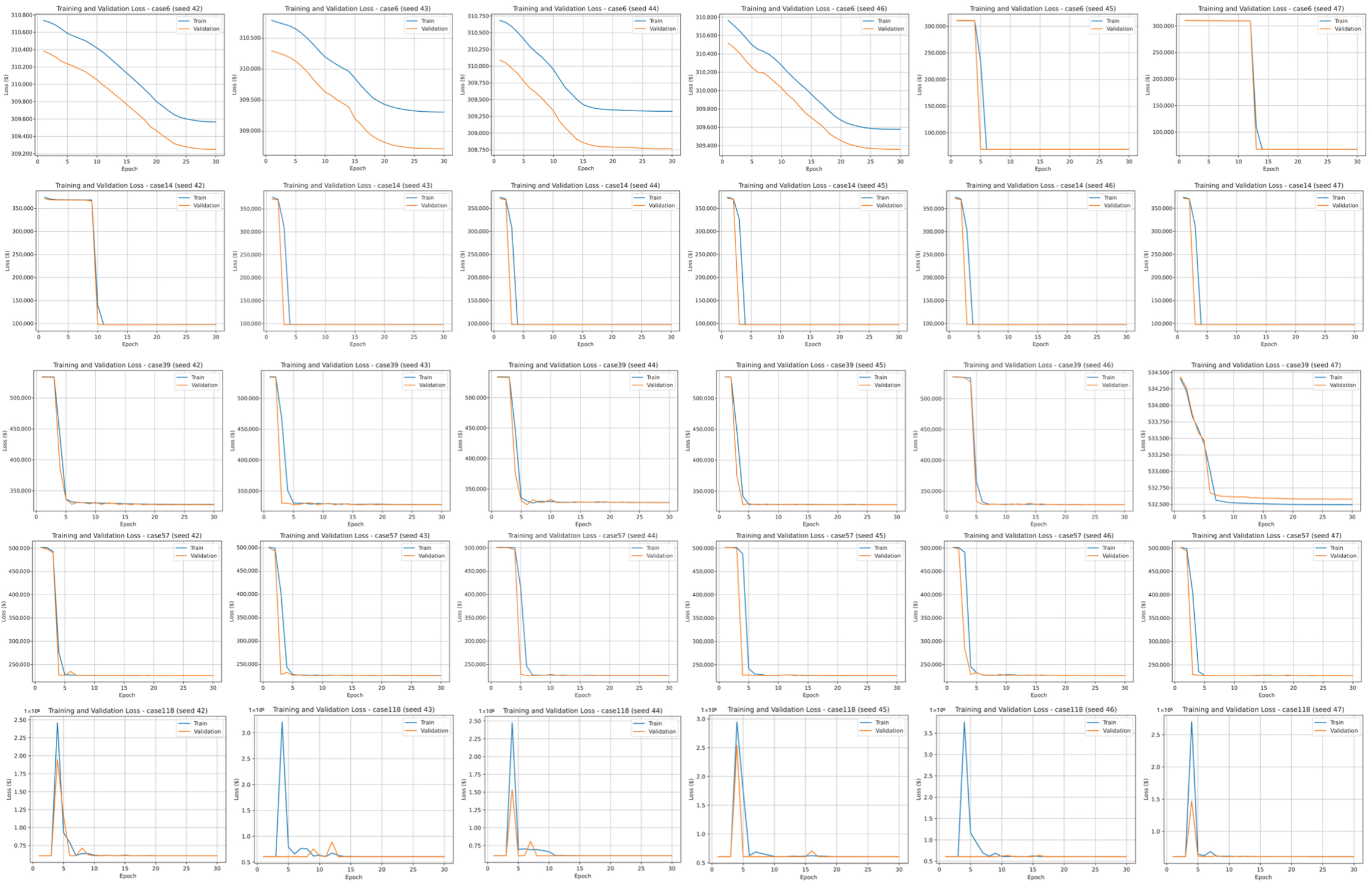
Figure 2 shows both the training and validation loss curves for each system. In the early stages of training, due to the presence of constraint penalty terms, the loss value is relatively high; as the iteration progresses, the network gradually learns to generate feasible solutions and reduce operating costs, which results in a steady decrease in losses. After approximately 25 rounds, all systems converged to a stable value, and no significant overfitting was observed.

Figure 2. Training Loss of Each System.

3.3. Accuracy and Feasibility of D-PGNet

Table 3 shows, for each of the five test sets, the mean ± standard deviation of the optimality gap and the maximum violation. The average optimality gap of all systems is within 1.08%, and all gaps are positive, indicating that the network has not achieved false lower costs due to constraint violations.

Table 3. Average Result of D-PGNet.

System	Average Cost (Net, $)	Average Cost (CVX, $)	Gap (%)	Maximum Constraint Violation (p.u.)
Case 6	69,124.93 ± 98.46	68,389.87 ± 111.28	1.075	0.0000126
Case 14	97,481.84 ± 127.66	96,878.51 ± 141.40	0.623	0.0000001
Case 39	334,643.26 ± 732.07	332,227.18 ± 418.88	0.727	0.0000024
Case 57	228,851.44 ± 260.86	227,878.22 ± 277.56	0.427	0.0000002
Case 118	2,649,951.51 ± 3745.78	2,642,560.88 ± 3745.26	0.280	0.0000023

Table 4 summarizes the individual constraint violations. Generator output limits and ramp constraints exhibit exactly zero violations across all test systems, confirming that the projection layer enforces these hard constraints perfectly. Overall, all violations remain below 1.3 × 10⁻⁵, which satisfies the practical accuracy requirements and validates the proposed end-to-end training and projection layer embedding strategy, indicating that the network has learned to satisfy constraints.

Table 4. Individual Constraint Violations.

System	PB	Pghigh	Pglow	Rampup	Rampdn	SOCeq	SOCter
Case 6	1.08 × 10−6	0.00 × 100	0.00 × 100	0.00 × 100	0.00 × 100	1.26 × 10−5	9.93 × 10−8
Case 14	1.19 × 10−7	0.00 × 100	0.00 × 100	0.00 × 100	0.00 × 100	4.08 × 10−8	0.00 × 100
Case 39	2.78 × 10−7	0.00 × 100	0.00 × 100	0.00 × 100	0.00 × 100	2.37 × 10−6	3.60 × 10−8
Case 57	1.19 × 10−7	0.00 × 100	0.00 × 100	0.00 × 100	0.00 × 100	2.08 × 10−7	3.23 × 10−8
Case 118	2.58 × 10−7	0.00 × 100	0.00 × 100	0.00 × 100	0.00 × 100	2.30 × 10−6	1.12 × 10−8

3.4. Solving Acceleration of D-PGNet

Table 5 compares the average single-sample inference time and CVXPY solution time of each system’s D-PGNet. Due to the parallel inference and lightweight projection of neural networks, the inference time of D-PGNet is, on average, three times faster than that of CVXPY. As the scale increases, the average solution time of D-PGNet is around 200 ms. On the 54-generator system of IEEE 118, the acceleration ratio can reach 64 times, highlighting the speed advantage of D-PGNet in large-scale problems.

Table 5. Computing Acceleration of D-PGNet.

System	Average Computing Time (Net, ms)	Average Computing Time (CVX, ms)	Speedup Ratio
Case 6	316.16	1609.86	5.1×
Case 14	318.08	1023.39	3.2×
Case 39	318.62	1350.98	4.0×
Case 57	337.33	856.63	2.6×
Case 118	358.21	22,886.93	64.8×

3.5. Comparison of Carbon Emissions and Wind Power Consumption

To further evaluate the environmental benefits of the scheduling scheme, we calculated the average total carbon emissions and wind power consumption rate of each system’s D-PGNet and CVXPY reference solutions, as presented in Table 4. The carbon emissions are obtained by multiplying the output of each unit in each period by the carbon emission coefficient and summing them up. The wind power consumption rate is defined as the ratio of the actual consumption power to the total available wind power.

From Table 6, it can be seen that the carbon emissions of D-PGNet are basically consistent with the CVXPY reference solution, with an average deviation of less than 0.2%, and this deviation is smaller than the objective function value, which indicates that the carbon emission cost in the low-carbon scheduling model plays a significant role in the network training and the network can accurately reproduce the low-carbon scheduling strategy. The wind power consumption rate remains at a high level (>99.88%) in all systems, and the results of the two methods are almost indistinguishable, which indicates that the proposed method is comparable to the performance of the exact solver in promoting renewable energy consumption. Considering the cost comparison in Table 2 and the speed comparison in Table 3, D-PGNet significantly reduces computation time while ensuring economy and environmental friendliness, which makes it suitable for real-time scheduling scenarios in large systems.

Table 6. Carbon Emissions and Wind Power Consumption Comparison.

System	Carbon Emissions (Net, t)	Carbon Emissions (CVX, t)	Wind Power Consumption Rate (Net, %)	Wind Power Consumption Rate (CVX, %)
Case 6	2161.58	2155.81	100.00	100.00
Case 14	3021.10	3018.14	99.99	100.00
Case 39	10,234.36	10,225.26	99.92	100.00
Case 57	7115.57	7107.78	99.88	100.00
Case 118	82,826.09	82,810.87	100.00	100.00

To analyze the effect of carbon pricing, we set a random carbon emission coefficient of 0.9 ± 0.2 and compared the dispatch under a baseline carbon price of $c_{\mathrm{carbon}}=30$ $/tCO₂ against the zero-carbon-price case. Table 7 reports the resulting total emissions and costs for the five test systems. With carbon pricing in effect, emissions decrease by approximately 13% on average, while the total system cost increases by about 8%, which indicates that carbon pricing effectively reduces emissions.

Table 7. Zero-Carbon Baseline Comparison.

System	Average Cost (${\mathit{c}}_{\mathbf{carbon}}=0$)	Average Cost—${\mathit{C}}_{\mathbf{carbon},\mathit{t}}$ (${\mathit{c}}_{\mathbf{carbon}}=30$)	Carbon Emissions (${\mathit{c}}_{\mathbf{carbon}}=0$)	Carbon Emissions (${\mathit{c}}_{\mathbf{carbon}}=30$)	ΔCost%	ΔEm%
Case 6	3715.85	4043.92	2078.46	2001.09	3.72	8.82
Case 14	6345.71	7180.59	3040.98	2727.42	10.31	13.15
Case 39	25,491	30,797.35	10,126.22	9126.49	9.87	20.81
Case 57	14,658.32	17,318.03	6904.95	6316.44	8.52	18.1
Case 118	158,412.8	168,835.17	83,412.69	75,198.5	9.84	6.57

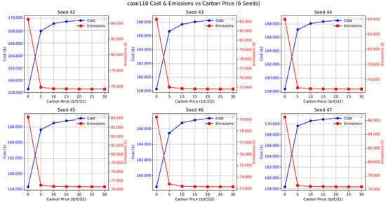
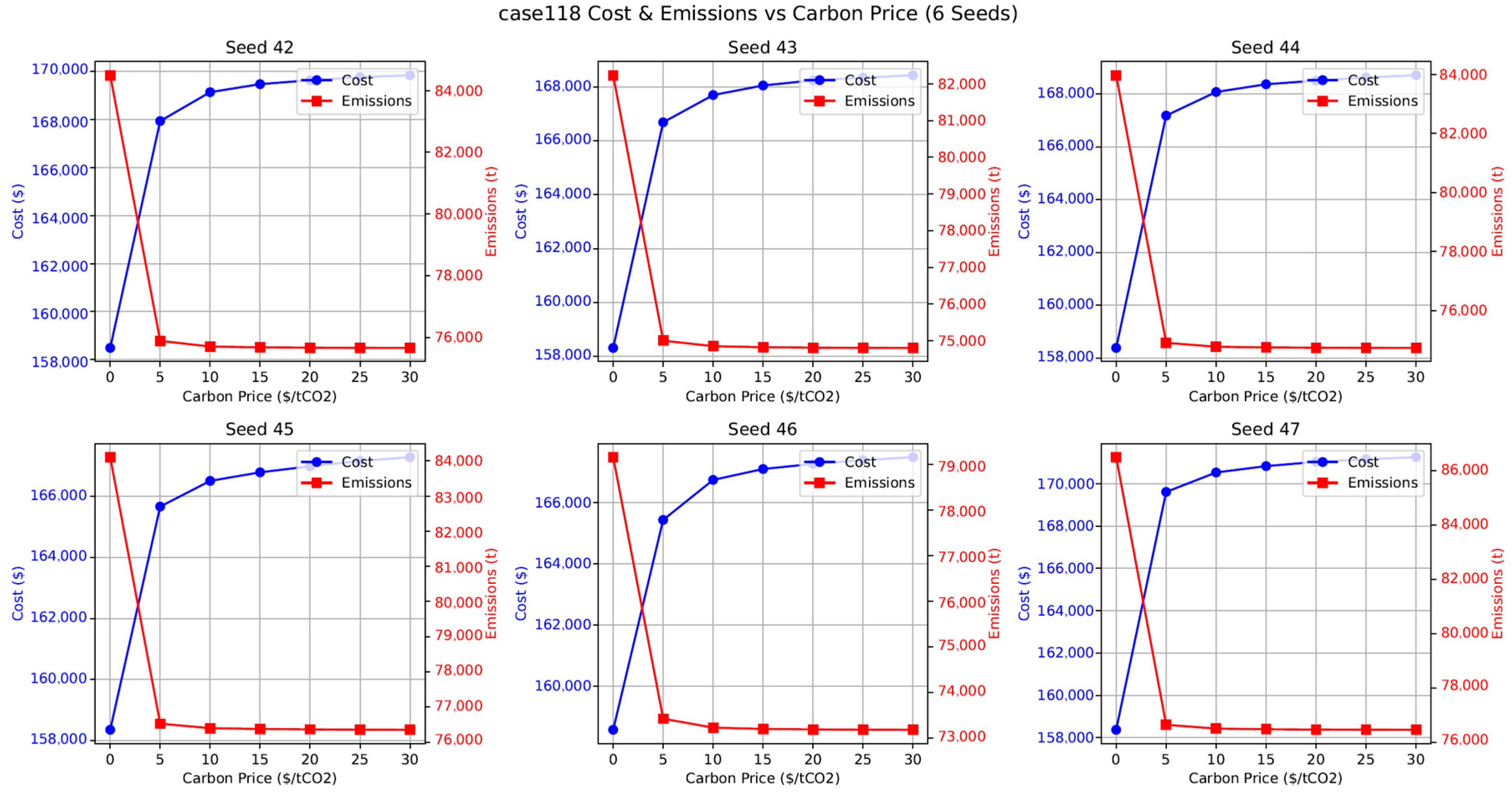
Figure 3 presents a sensitivity analysis on case 118, with $c_{\mathrm{carbon}}$ varying continuously from 0 to 30 $/tCO₂. The emission and cost trajectories display a clear nonlinear pattern: both emission reduction and cost increase are most pronounced when the carbon price is first introduced, and the marginal impact gradually diminishes as the price rises further. This is because, as the carbon price increases, the scheduling results gradually reach the minimum carbon emission value, which indicates that the carbon cost signal effectively steers the dispatch toward lower-carbon solutions.

Figure 3. Carbon Sensitivity.

4. Discussion

The superior performance of D-PGNet can be attributed to the explicit encoding of constraint geometry into the projection layers, which fundamentally differs from penalty-based physics-informed neural networks. Our method satisfies nearly all constraints without sacrificing solution optimality, because the Dykstra alternating projection mechanism actively pulls infeasible points back to the feasible manifold during training and inference. The use of self-supervised learning further eliminates the need for expensive labeled datasets, allowing the network to directly adapt to carbon price signals. Direct comparison with recent learning-based dispatch methods further contextualizes these results. Supervised predictors such as DeepOPF report constraint violations typically corrected by post-processing, which may compromise optimality; D-PGNet’s projection layers avoid this issue entirely. Reinforcement learning agents for real-time dispatch require extensive reward engineering to enforce constraints, whereas our method structurally guarantees near-feasibility. Among algorithm-unfolding frameworks, OptNet embeds a full QP solver and incurs cubic complexity, limiting scalability. By contrast, D-PGNet’s tailored Dykstra projections achieve linear complexity with exact closed-form updates, demonstrating a more favorable speed–feasibility trade-off for the low-carbon ED problem with storage. However, there are also limitations that point to the direction of future development.

The current D-PGNet relies on a DC power flow approximation; network losses, line flow limits, and voltage constraints are not modeled. Extending the framework to AC optimal power flow requires projecting onto non-convex power flow equations, which lack closed-form projections. A promising direction is to embed linearized power flow constraints directly into the projection layer or to use implicit-layer differentiation to enforce AC feasibility. Additionally, unit commitment integer variables are not considered; future work could integrate the unfolded network with learning-based branch-and-bound or relaxed rounding schemes.

While the current work employs a simplified energy storage model with constant efficiency, recent advances in solid-state electrolytes and two-dimensional materials are pushing battery performance boundaries [28,29,30]. Incorporating more accurate, data-driven battery degradation models into the proposed framework could further enhance its practical value for next-generation energy storage systems.

The linear carbon cost model assumes a uniform carbon price and ignores the allowances, multi-tier pricing, and quota trading constraints present in real emission trading systems. This simplification is widely adopted in the low-carbon dispatch literature for analytical tractability and is sufficient to demonstrate the efficacy of the proposed framework [31,32]. Extensions to include stepwise carbon prices or cap-and-trade constraints are straightforward from an optimization perspective and will be explored in future work.

5. Conclusions

This paper presents D-PGNet, a deep unfolding network based on projected gradient descent for low-carbon economic dispatch incorporating carbon emission costs, wind power, and energy storage. A differentiable Dykstra alternating projection layer enforces power balance, ramp-rate, and full energy storage dynamics, yielding solutions with constraint violations below 1.3 × 10⁻⁵ p.u. The self-supervised loss embeds the carbon trading cost directly, enabling label-free learning of low-carbon strategies. Numerical results show optimality gaps under 1.08% and an over 64-fold speed-up versus conventional solvers, with robust performance across multiple system scales. This work validates the effectiveness of algorithm unfolding for power system optimization and offers a practical pathway toward real-time, carbon-aware dispatch in future clean energy systems.

References

- Lu, Z.; Yan, L.; Wang, J.; Kang, C.; Shahidehpour, M.; Li, Z. A Market-Clearing-Based Sensitivity Model for Locational Marginal and Average Carbon Emission. IEEE Trans. Energy Mark. Policy Regul. 2024, 2, 579–582. [Google Scholar] [CrossRef]
- State Council of the People’s Republic of China. Regulation on the Administration of Carbon Emission Trading; State Council of the People’s Republic of China: Beijing, China, 2024.
- Jin, J.; Zhou, P.; Li, C.; Guo, X.; Zhang, M. Low-carbon power dispatch with wind power based on carbon trading mechanism. Energy 2019, 170, 250–260. [Google Scholar] [CrossRef]
- Lu, Z.; Yan, L.; Li, Z.; Xiao, Y.; Shahidehpour, M.; Wang, X. Convex-Hull of Locational Marginal Carbon Emission for Carbon Management Considering Emissions during Non-Steady-State Operation Hours. IEEE Trans. Smart Grid. 2026, 17, 3083–3098. [Google Scholar] [CrossRef]
- Meng, Y.; Yan, L.; Mei, L.; Lu, Z.; Yan, G.; Feng, Y. Incentive-compatible Flexibility Sharing for Enhancing Controllability and Economic Efficiency of Demand Response. IEEE Trans. Smart Grid 2026, 17, 1940–1955. [Google Scholar] [CrossRef]
- Meng, Y.; Fan, S.; Shen, Y.; Xiao, J.; He, G.; Li, Z. Transmission and distribution net work-constrained large-scale demand response based on locational cus tomer directrix load for accommodating renewable energy. Appl. Energy 2023, 350, 121681. [Google Scholar] [CrossRef]
- Meng, Y.; Yan, L.; Li, Z.; Shahidehpour, M.; Zhang, Y.; Mei, L.; Shen, B.; Wang, J. Flexibility sharing for collaborative load regulation: Mechanism and solution. Appl. Energy 2026, 420, 128151. [Google Scholar] [CrossRef]
- Yan, G.; Yan, L.; Meng, Y.; Han, J.; Li, Z. Linear-Exponential Decay Frequency Curve for Unit-Specific Response in Frequency-Constrained Unit Commitment. IEEE Trans. Power Syst. 2026. Early Access. [Google Scholar] [CrossRef]
- Wang, J.; He, X.; Huang, J.; Chen, G. Recurrent Neural Network for Nonconvex Economic Emission Dispatch. J. Mod. Power Syst. Clean Energy 2021, 9, 46–55. [Google Scholar] [CrossRef]
- Fu, Y.; Shahidehpour, M.; Li, Z. AC contingency dispatch based on security-constrained unit commitment. IEEE Trans. Power Syst. 2006, 21, 897–908. [Google Scholar] [CrossRef]
- Momoh, J.; Mili, L. (Eds.) Operation and Control of Electric Energy Processing Systems; IEEE Press: Piscataway, NJ, USA; Wiley: Hoboken, NJ, USA, 2010. [Google Scholar]
- Huang, G.; Wu, F.; Guo, C. Smart grid dispatch powered by deep learning: A survey. Front. Inf. Technol. Electron. Eng. 2022, 23, 763–776. [Google Scholar] [CrossRef]
- Zhang, Q.; Luo, W.; Yan, R.; Geng, G.; Jiang, Q. Policy-Assisted Graph Reinforcement Learning for Real-Time Economic Dispatch. J. Mod. Power Syst. Clean Energy 2025, 13, 1896–1908. [Google Scholar]
- Pan, X.; Zhao, T.; Chen, M. DeepOPF: A deep neural network approach for security-constrained DC optimal power flow. IEEE Trans. Power Syst. 2021, 36, 1885–1895. [Google Scholar] [CrossRef]
- Chen, T.; Chen, X.; Chen, W.; Heaton, H.; Liu, J.; Wang, Z.; Yin, W. Learning to optimize: A primer and a benchmark. J. Mach. Learn. Res. 2022, 23, 1–59. [Google Scholar] [CrossRef]
- Gregor, K.; LeCun, Y. Learning fast approximations of sparse coding. In Proceedings of the 27th International Conference on Machine Learning (ICML), Haifa, Israel, 21–24 June 2010; pp. 399–406. [Google Scholar]
- Dong, W.; Zhang, F.; Li, M.; Fang, X.; Yang, Q. Imitation Learning Based Real-Time Decision-Making of Microgrid Economic Dispatch Under Multiple Uncertainties. J. Mod. Power Syst. Clean Energy 2024, 12, 1183–1193. [Google Scholar]
- Liu, J.; Chen, X. ALISTA: Analytic weights are as good as learned weights in LISTA. In Proceedings of the International Conference on Learning Representations (ICLR), New Orleans, LA, USA, 6–9 May 2019. [Google Scholar]
- Zhang, J.; Ghanem, B. ISTA-Net: Interpretable optimization-inspired deep network for image compressive sensing. In Proceedings of the IEEE/CVF Conference on Computer Vision and Pattern Recognition (CVPR), Salt Lake City, UT, USA, 18–22 June 2018; pp. 1828–1837. [Google Scholar]
- Sun, J.; Li, H.; Xu, Z. Deep ADMM-Net for compressive sensing MRI. In Advances in Neural Information Processing Systems (NeurIPS), Barcelona, Spain, 5–10 December 2016; Curran Associates, Inc.: Red Hook, NY, USA, 2016; pp. 10–18. [Google Scholar]
- Fioretto, F.; Mak, T.W.K.; Van Hentenryck, P. Predicting AC optimal power flows: Combining deep learning and Lagrangian dual methods. In Proceedings of the AAAI Conference on Artificial Intelligence, New York, NY, USA, 7–12 February 2020; pp. 6349–6356. [Google Scholar]
- Drgoňa, J.; Kiš, K.; Tuor, A.; Vrabie, D.; Klaučo, M. Differentiable predictive control: Deep learning alternative to explicit model predictive control for unknown nonlinear systems. J. Process Control 2022, 116, 80–92. [Google Scholar]
- Boyd, S.; Vandenberghe, L. Convex Optimization; Cambridge University Press: Cambridge, UK, 2004. [Google Scholar]
- Amos, B.; Kolter, J.Z. OptNet: Differentiable optimization as a layer in neural networks. In Proceedings of the 34th International Conference on Machine Learning (ICML), Sydney, Australia, 6–11 August 2017; pp. 136–145. [Google Scholar]
- Bauschke, H.H.; Borwein, J.M. On projection algorithms for solving convex feasibility problems. SIAM Rev. 1996, 38, 367–426. [Google Scholar] [CrossRef]
- Bauschke, H.H.; Borwein, J.M. Dykstra’s alternating projection algorithm for two sets. J. Approx. Theory 1994, 79, 418–443. [Google Scholar] [CrossRef]
- Condat, L. Fast projection onto the simplex and the ℓ1 ball. Math. Program. 2016, 158, 575–585. [Google Scholar] [CrossRef]
- Chen, T.; Reddy, N.P.; Li, M. Enhancing Solid-State Li-Ion Batteries with MOF-Polymer Composite Electrolytes-Effect Mechanisms and Interface Engineering. Gels 2025, 11, 946. [Google Scholar] [CrossRef] [PubMed]
- Zhao, D.; Liu, C.; Chen, T.; Li, M. Recent Advances in Aqueous Zinc Ion Batteries: Energy Storage Mechanisms, Challenges, and Optimization Strategies. Batteries 2026, 12, 109. [Google Scholar] [CrossRef]
- Mouli, K.V.V.C.; Mani, D.; Ramachandran, T.; Kumar, Y.A.; Ghosh, A.; Somu, P.; Mangiri, R. A New Era in Energy Storage: In Situ and Operando Characterization of 2D Materials-Based Devices. Mater. Chem. Phys. 2025, 348, 131660. [Google Scholar] [CrossRef]
- Lu, H.; Chang, X.; Xue, Y.; Tian, X.; Xu, J.; Sun, H. Carbon Entropy-Based Two-Stage Low-Carbon Dispatch for Distribution Networks with LSTM Load Forecasting. In 2025 IEEE 9th Conference on Energy Internet and Energy System Integration (EI2); IEEE: New York, NY, USA, 2025; pp. 2901–2907. [Google Scholar]
- Rho, S.; Moon, H.S.; Park, W.Y.; Won, D. Optimal dispatch and impact analysis of power–heat–gas integrated energy systems considering carbon pricing schemes. Appl. Energy 2025, 45, 102079. [Google Scholar] [CrossRef]
Disclaimer/Publisher’s Note: The statements, opinions and data contained in all publications are solely those of the individual author(s) and contributor(s) and not of MDPI and/or the editor(s). MDPI and/or the editor(s) disclaim responsibility for any injury to people or property resulting from any ideas, methods, instructions or products referred to in the content. |
© 2026 by the authors. Licensee MDPI, Basel, Switzerland. This article is an open access article distributed under the terms and conditions of the Creative Commons Attribution (CC BY) license.