An Optimization Approach to Select Koopman Observables for Data-Based Modeling Using Dynamic Mode Decomposition with Control

Abstract

The advent and evolution of Industry 4.0 have been driven by technologies such as the Industrial Internet of Things, Big Data, and Cloud Computing. Within this framework, digital twins have gained significant popularity and are now employed across a wide range of industries and processes. A crucial step in developing a digital twin is deriving the system model, for which numerous methods are available. Among these, the Koopman operator and Dynamic Mode Decomposition with control have demonstrated their effectiveness and are widely recognized in the scientific community. This paper proposes a procedure for the automatic selection of Koopman observables by solving an optimization problem. The objective is to identify the minimal set of observables, belonging to a predefined dictionary, that minimize the error between actual process observations and predictions made by the estimated linear model—a key requirement for digital twin development. To tackle the optimization challenge, any algorithm available in the literature can be utilized. In this paper, the evolutive algorithms, including Genetic Algorithm and Differential Evolution Algorithm, are applied to evaluate the proposed approach in a benchmark problem. In both cases, the algorithms obtained the minimum set of observable functions from the dictionary used that achieve the lowest error obtained between the real process and the model, confirming the validity of the proposed method.

1. Introduction

Industry 4.0 marks the fourth industrial revolution, driven by the convergence of digital, physical, and biological systems. It represents a transformative paradigm in modern manufacturing and industrial processes, characterized by the seamless integration of advanced technologies such as the Industrial Internet of Things (IIoT), Artificial Intelligence (AI), Cloud Computing, and Big Data analytics. The core objective here is to create smart factories where machines, devices, and humans are interconnected, enabling real-time data exchange and decision-making. The implementation of technologies associated with this paradigm enhances productivity, efficiency, and agility across various sectors. It enables condition monitoring [1,2], predictive maintenance [3], flexibility and safety [4,5], supply chain optimization [6], and mass customization [7], empowering industries to respond quickly to changing market demands.

One of the most transformative technologies within the Industry 4.0 framework is the concept of digital twins [8,9,10,11,12]. As Industry 4.0 emphasizes the integration of physical and digital systems, digital twins serve as the bridge between these two realms. According to [13], a digital twin is a representation of a physical object or process in a virtual environment. It continuously receives data from Internet of Things (IoT) sensors and other sources, enabling it to reflect the current state, predict future behavior, and simulate potential outcomes. They allow industries to shift from reactive to predictive strategies, enabling proactive maintenance, process optimization, and design iteration without disrupting real-world operations. By simulating different scenarios and predicting future states, digital twins enable industries to make informed decisions, reduce downtime, and accelerate innovation in an increasingly complex and interconnected industrial landscape. Consequently, this technology has become an attractive tool for industries seeking to achieve greater flexibility, resilience, and sustainability in an increasingly competitive landscape.

The development of robust system-modeling frameworks that leverage digital twin technology is crucial for achieving the full potential of Industry 4.0. This will require the integration of multiple technologies, like IoT for data acquisition, AI for predictive analytics, and Cloud Computing for scalable processing. Furthermore, the development of digital twin models must consider computational efficiency, as real-time simulation and decision-making are critical in Industry 4.0 environments. These models must strike a balance between detail and computational load, ensuring they are both accurate and fast enough to provide actionable insights when needed.

In this context, dynamic system modeling is crucial for a wide range of applications, including process control, system simulation, behavior prediction, and operational optimization. Unlike traditional methods that rely solely on analytical models derived from physical equations, data-based approaches offer a powerful alternative by utilizing large volumes of real-time data that are obtained thanks to the technological advances of the fourth industrial revolution, to construct accurate models without needing a detailed understanding of the underlying dynamics. Data-based modeling is particularly useful for nonlinear systems, which are commonly found in complex industrial applications such as automation [14], robotics [15], energy management [16], and machinery behavior prediction [17].

Related to digital twins and Industry 4.0, the Koopman operator emerges as a powerful mathematical tool to significantly enhance the data-based modeling of industrial systems. The Koopman theory provides a robust tool for analyzing nonlinear dynamical systems by transforming them into a higher-dimensional space where the dynamics are linearized [18]. This transformation allows for the study of nonlinear systems using linear methods, making the Koopman operator an attractive approach for model reduction, control, and prediction in complex systems. Some fields of application for this technique include robotics [19], the automotive industry [20], systems control [21], among others.

While the Koopman operator offers a robust framework for analyzing nonlinear systems by transforming them into a higher-dimensional linear space, its practical application to real-world systems often requires an efficient way to extract the relevant information from data. This is where Dynamic Mode Decomposition (DMD) comes into play [18], offering a data-driven approach [22] to approximate the Koopman operator’s dynamics directly from measurements of the system’s states. This method provides an approximate spectral decomposition of the system dynamics, capturing both oscillatory and exponential modes. DMD-based algorithms have been used in various types of applications: fluid studies [23], aircraft parameter estimation [22], temperature analysis in smart buildings [24], among others.

However, classical DMD assumes that the system is governed by a linear evolution, which can limit its accuracy when modeling systems with external control inputs or nonlinear dynamics. To address the first challenge, Dynamic Mode Decomposition with control (DMDc) extends the classical DMD framework by incorporating control inputs into the modeling process [25], thus offering a more comprehensive tool for analyzing and predicting the dynamics of controlled systems. To tackle the second challenge, a generalization of DMD known as Extended Dynamic Mode Decomposition (EDMD) was proposed in [26]. In this case, the aim is to find the set of eigenfunctions, eigenvectors, and eigenvalues of the Koopman operator from a finite approximation of it, which allows for the determination of the system’s time response.

In recent years, the trend within the field of system modeling has increasingly favored the use of EDMD with Koopman theory. One of the main challenges in applying the Koopman operator is the selection of the right set of observables. The choice of observables determines the accuracy and efficiency of the Koopman model, and there is no universal or automatic method for selecting them, which is the main research problem motivating this work. Many related works focus on different ways to find an approximation of the Koopman operator and accordingly select the observables based on what we might identify as expert knowledge [27,28,29,30]. However, in contrast to the prevalent trend of employing EDMD with the Koopman theory [31,32,33,34], this paper proposes a divergent approach to system modeling. This method aims to derive the matrices $\mathbf{A}$ and $\mathbf{B}$ of the discrete linear system model, thereby enabling the use of various types of techniques that are widely employed for system analysis and controller design.

This work aims to present a novel approach for automatically selecting Koopman observables by addressing an optimization problem, which constitutes its primary scientific contribution. The proposed method identifies the minimal set of observables that minimizes the discrepancy (error) between the actual process measurements and those predicted by the estimated linear model. By taking this approach, experts will obtain the set of functions that best describe the nonlinearities of the process (in the context of a predefined dictionary of observables), providing valuable support for a more in-depth understanding and analysis of the underlying dynamics of the study system. To address this optimization challenge, any of the many algorithms available in the literature can be employed. In this study, two evolutionary algorithms, Genetic Algorithm (GA) and Differential Evolution (DE), are used to evaluate the proposed approach. To assess their performance, the algorithms were applied to the modeling of a continuously stirred tank reactor (CSTR) taken from [35]. In both cases, the algorithms obtained the minimum set of observable functions from the dictionary used that achieve the lowest error between the real process and the model that is obtained, confirming the validity of the proposed method. Furthermore, a possible practical implementation architecture of the proposed approach is presented, which constitutes another contribution.

The paper is organized as follows: Section 2 presents the main results obtained in the study of the background of data-driven modeling of dynamical systems using the Koopman operator theory. Section 3 describes the fundamental characteristics of the tools used, the proposed methodology, and the case study; Section 4 shows the experimental design for testing the proposed approach and the analysis of the results obtained; Section 5 focuses on the practical application of the proposed procedure within an industrial context. Finally, the Conclusions are presented.

2. Related Works

Data-driven dynamical system analysis remains a prominent topic today. Although Koopman theory has been actively investigated during the past decade, its relevance continues to be significant. Based on the Koopman operator, Koopman theory provides a mathematical framework for analyzing nonlinear dynamical systems by transforming them into a higher-dimensional space where their dynamics can be represented linearly [18]. Instead of working directly with the nonlinear state space, Koopman theory works on a space of observables. This space of observables consists of functions of the state variables that provide a linear description in the transformed space, even when the underlying system remains nonlinear. By extending the analysis to a theoretically infinite higher-dimensional space of these observables, the Koopman operator enables the decomposition of complex, nonlinear dynamics into interpretable linear representations. Consequently, it serves as a powerful tool for modeling nonlinear systems.

Although the Koopman operator maps to an infinite-dimensional space, practical implementation requires finite-dimensional approximations. Some researchers are exploring a linear parameter-varying Koopman model [36]. In this context, it is assumed that the representation of the Koopman operator is linear but parameter-dependent. Essentially, this approach generalizes the Koopman operator to incorporate dependencies on a set of time-varying parameters. Other researchers are investigating transfer learning strategies [37]. There is also a trend for Koopman linear flow estimators [38], which focus on estimating the dynamics of observables that evolve linearly within the Koopman framework. However, another more widely adopted approach for approximating the Koopman operator is DMD, particularly EDMD [39,40,41].

Related to DMD and its variants, there is a research gap that remains open: the selection of an appropriate dictionary of observables. There are two main groups of research fields to tackle this limitation. One group bases its proposals on neural network architectures [42,43,44,45]. In this trend, instead of selecting the set of basis functions randomly [42], neural networks are used as learned observables that generate the Koopman space. The second group follows the approach of the classical EDMD method with predefined dictionaries. In this group, many related works focus on different ways to accordingly select the observables based on what we might identify as expert knowledge [27,28,29,30]. Additionally, there is also an open research field that allows for the refinement of the dictionary [46] by using a Tunable Symmetric Subspace Decomposition algorithm.

To the best of our knowledge, after conducting a literature review, there is no procedure capable of automatically selecting the minimal set of Koopman observables from a predefined dictionary of functions that minimizes the error between the behavior of the variables of the actual process and the results of the obtained model. Consequently, the fundamental contribution of this paper lies in presenting a novel method that identifies the minimal set of Koopman observables that most effectively minimize the error associated with simulated samples of the system model obtained through DMDc. Our proposal can be seen as a DMD-based Koopman approximation approach, with a predefined dictionary, that optimally selects the best and smallest set of observables. This method utilizes popular strategies within the Koopman theory framework and also employs data-driven optimization techniques to overcome the tedious, complex, and mostly manual selection of observables. This also ensures that the user of the procedure does not require a deep knowledge of the studied system.

3. Materials and Methods

In this section, the theoretical foundations of the mathematical tools, DMDc and the Koopman operator, upon which the proposal in this paper is based, will be presented. Subsequently, the methodology is proposed based on the solution of an optimization problem for the automatic selection of the smallest set of Koopman observables that minimize the error between the real process and the model obtained by applying DMDc. Following that, the general characteristics of the algorithms GA and DE are described, along with the test problem that is used to evaluate the proposed methodology.

3.1. Dynamic Mode Decomposition with Control

DMD is a data analysis technique used to identify dynamic systems from experimental data. It allows for the use of high-dimensional sampled data from processes to extract coherent structures that contain the dominant characteristics of their dynamical behavior [47]. However, as mentioned above, traditional DMD methods have limitations when applied to systems under control, particularly in the context of Industry 4.0 applications, where real-time control inputs are often integral to system behavior. DMDc builds upon DMD by integrating control inputs into the framework [25]. Specifically, it introduces control as an additional variable in the decomposition, allowing the method to model systems where the state evolution is influenced not only by internal dynamics but also by external control actions.

Consider a discrete system that evolves over time; its measurements are given by states ${\mathbf{x}}_j$ at discrete times j, and the influence of a control input is given by ${\mathbf{u}}_j$. The idea is to identify the matrices $\mathbf{A}$ and $\mathbf{B}$ that describe the system’s dynamics according to the following relationship:

$$\begin{array}{cc}\hfill {\mathit{x}}_{j+1}& =\mathbf{A}{\mathit{x}}_j+\mathbf{B}{\mathit{u}}_j\hfill \end{array}$$

(1)

$$\begin{array}{cc}\hfill {\mathit{y}}_{j+1}& =\mathbf{C}{\mathit{x}}_{j+1}\hfill \end{array}$$

(2)

where $\mathbf{A}\in {\mathbb{R}}^{n\times n}$, $\mathbf{B}\in {\mathbb{R}}^{n\times m}$ and $\mathbf{C}\in {\mathbb{R}}^{h\times n}$, with n being the dimension of the system, m the number of inputs, and h the number of outputs. On the other hand, the vector ${\mathit{y}}_{j+1}$ represents the outputs of the process.

The system measurements and control inputs can be represented as follows:

$${\mathbf{X}}_0=[{\mathbf{x}}_0,{\mathbf{x}}_1,{\mathbf{x}}_2,\dots ,{\mathbf{x}}_{p-1}]$$

(3)

$$\mathbf{U}=[{\mathbf{u}}_0,{\mathbf{u}}_1,{\mathbf{u}}_2,\dots ,{\mathbf{u}}_{p-1}]$$

(4)

$${\mathbf{X}}_1=[{\mathbf{x}}_1,{\mathbf{x}}_2,{\mathbf{x}}_3,\dots ,{\mathbf{x}}_p]$$

(5)

Here, ${\mathbf{X}}_0$ and ${\mathbf{X}}_1$ are matrices that contain the sequences of system states, and $\mathbf{U}$ is the control input matrix. Now, Equation (1) can be rewritten as:

$${\mathbf{X}}_1=\mathbf{A}{\mathbf{X}}_0+\mathbf{B}\mathbf{U}$$

(6)

In summary, the steps to follow for the application of DMDc are [18]:

• Data Collection: build the matrices ${\mathbf{X}}_0$, ${\mathbf{X}}_1$, and $\mathbf{U}$ from the system measurements.
• Formation of $\mathbf{Z}$: stack the matrices ${\mathbf{X}}_0$ and $\mathbf{U}$ into a single matrix $\mathbf{Z}$:

  $$\mathbf{Z}=\left[\begin{array}{c}{\mathbf{X}}_0\\ \mathbf{U}\end{array}\right]$$

  (7)
• Singular value decomposition (SVD): perform the SVD of the matrix $\mathbf{Z}$:

  $$\mathbf{Z}\approx U_{svd}{\Sigma }_{svd}{V_{svd}}^{*}=\left[\begin{array}{c}{U}_{sv{d}_1}\\ U_{sv{d}_2}\end{array}\right]{\Sigma }_{svd}{V_{svd}}^{*}$$

  (8)

  where * indicates the conjugate transpose of the matrix.
• Obtain $\mathbf{A}$ and $\mathbf{B}$: obtain the matrices $\mathbf{A}$ and $\mathbf{B}$ from the linear system:

  $$\left[\begin{array}{cc}\mathbf{A}& \mathbf{B}\end{array}\right]\approx {\mathbf{X}}_1{\left[\begin{array}{c}{\mathbf{X}}_0\\ U\end{array}\right]}^{†}=\left[\begin{array}{cc}{\mathbf{X}}_1{V}_{svd}{{\Sigma }_{svd}}^{-1}{U_{sv{d}_1}}^{*}& {\mathbf{X}}_1{V}_{svd}{{\Sigma }_{svd}}^{-1}{U_{sv{d}_2}}^{*}\end{array}\right]$$

  (9)

  where † is the Moore–Penrose pseudoinverse.

3.2. The Koopman Operator

Koopman theory is a powerful framework in the field of dynamical systems that enables the study of nonlinear dynamics from a linear perspective. It basically proposes that any nonlinear system can be approximated by an infinite-dimensional linear system [18].

For practical applications, consider a discrete-time dynamical system with states ${\mathbf{x}}_j$ at discrete time steps j. The goal is to analyze the system using observables $\mathbf{g}\left(\mathbf{x}\right)$, which are functions that map the state space to a higher-dimensional space. These observables can capture the essential dynamics of the system. The state measurements and the corresponding observables can be represented as:

$$\mathbf{X}=[{\mathbf{x}}_0,{\mathbf{x}}_1,{\mathbf{x}}_2,\dots ,{\mathbf{x}}_p]$$

(10)

$$\mathbf{G}=[\mathbf{g}\left({\mathbf{x}}_0\right),\mathbf{g}\left({\mathbf{x}}_1\right),\mathbf{g}\left({\mathbf{x}}_2\right),\dots ,\mathbf{g}\left({\mathbf{x}}_p\right)]$$

(11)

Here, $\mathbf{X}$ represents the sequence of states, and $\mathbf{G}$ represents the corresponding observables.

The Koopman operator $\mathcal{K}$ acts on the space of observables and describes their evolution over time. For a given observable $\mathbf{g}\left(\mathbf{x}\right)$, the Koopman operator is defined as:

$$\mathcal{K}\mathbf{g}\left({\mathbf{x}}_k\right)=\mathbf{g}\left(\mathbf{f}\left({\mathbf{x}}_k\right)\right)$$

(12)

where $\mathbf{f}\left({\mathbf{x}}_k\right)$ represents the dynamics of the system. This operator is linear, even if the underlying system dynamics are nonlinear.

As mentioned above, DMDc cannot specifically address the limitations of nonlinear systems. However, it translates the Koopman operator framework into a computationally accessible tool. DMDc bypasses the explicit construction of the Koopman operator, and its simplicity is particularly advantageous for digital twin development, where computational efficiency and model accuracy are essential. In the context of a controlled system:

$${\mathbf{x}}_{j+1}=\mathbf{f}({\mathbf{x}}_j,{\mathbf{u}}_j),$$

(13)

So, now the Koopman operator framework leads to the following dynamical equation:

$$\mathcal{K}\mathbf{g}\left({\mathbf{x}}_{j+1}\right)=\mathbf{g}\left(\mathbf{f}({\mathbf{x}}_j,{\mathbf{u}}_j)\right)$$

(14)

The approximate evolution of the observables for this new system is:

$$\mathbf{g}\left({\mathbf{x}}_{j+1}\right)=\mathbf{A}\mathbf{g}\left({\mathbf{x}}_j\right)+\mathbf{B}{\mathbf{u}}_j$$

(15)

Similarly to DMDc mechanism, the process of obtaining the matrices $\mathbf{A}$ and $\mathbf{B}$ involves the construction of data matrices from sampled observations of the system’s evolution and the application of the SVD. Here is a step-by-step guide to this process:

• Data Collection: keep matrix $\mathbf{U}$, and from matrices ${\mathbf{X}}_0$ and ${\mathbf{X}}_1$ form ${\mathbf{G}}_0$ and ${\mathbf{G}}_1$, respectively:

  $${\mathbf{G}}_0=[\mathbf{g}\left({\mathbf{x}}_0\right),\mathbf{g}\left({\mathbf{x}}_1\right),\mathbf{g}\left({\mathbf{x}}_2\right),\dots ,\mathbf{g}\left({\mathbf{x}}_{p-1}\right)]$$

  (16)

  $${\mathbf{G}}_1=[\mathbf{g}\left({\mathbf{x}}_1\right),\mathbf{g}\left({\mathbf{x}}_2\right),\mathbf{g}\left({\mathbf{x}}_3\right),\dots ,\mathbf{g}\left({\mathbf{x}}_p\right)]$$

  (17)
• Formation of $\mathbf{H}$: stack the matrices ${\mathbf{G}}_0$ and $\mathbf{U}$ into a single matrix $\mathbf{H}$:

  $$\mathbf{H}=\left[\begin{array}{c}{\mathbf{G}}_0\\ \mathbf{U}\end{array}\right]$$

  (18)
• Perform the SVD of the matrix $\mathbf{H}$:

  $$\mathbf{H}\approx U_{sv{d}_{\mathrm{K}}}{\Sigma }_{sv{d}_{\mathrm{K}}}{V_{sv{d}_{\mathrm{K}}}}^{*}=\left[\begin{array}{c}{U}_{sv{d}_1\mathrm{K}}\\ U_{sv{d}_2\mathrm{K}}\end{array}\right]{\Sigma }_{svd}{V_{sv{d}_{\mathrm{K}}}}^{*}$$

  (19)

  where * indicates the conjugate transpose of the matrix.
• Obtain $\mathbf{A}$ and $\mathbf{B}$: obtain the matrices $\mathbf{A}$ and $\mathbf{B}$ from the linear system:

  $$\left[\begin{array}{cc}\mathbf{A}& \mathbf{B}\end{array}\right]\approx {\mathbf{G}}_1{\left[\begin{array}{c}{\mathbf{G}}_0\\ U_{sv{d}_{\mathrm{K}}}\end{array}\right]}^{†}=\left[\begin{array}{cc}{\mathbf{G}}_1{V}_{sv{d}_{\mathrm{K}}}{{\Sigma }_{sv{d}_{\mathrm{K}}}}^{-1}{U_{sv{d}_1\mathrm{K}}}^{*}& {\mathbf{G}}_1{V}_{sv{d}_{\mathrm{K}}}{{\Sigma }_{sv{d}_{\mathrm{K}}}}^{-1}{U_{sv{d}_2\mathrm{K}}}^{*}\end{array}\right]$$

  (20)

  where † is the Moore–Penrose pseudoinverse.

If Equations (9) and (20) are analyzed carefully, it can be seen that there is a close relationship between DMDc and the Koopman operator. By itself, DMDc cannot address the nonlinearities present in many real-world systems. However, by adopting the aforementioned methodology, this limitation can be overcome. This proposal bypasses the explicit construction of the Koopman operator and directly provides a linear approximation of the system dynamics.

3.3. Procedure for Optimal Selection of Koopman Observables

The procedure proposed in this paper to select the set of Koopman observable functions for obtaining a linear model of the analyzed process is based on the solution of an optimization problem. This approach has theoretical and practical advantages. First of all, optimization is intrinsically well-suited to the kind of problem where there is a necessity to select a minimal subset satisfying certain constraints or objectives, such as maximizing alignment with system dynamics. The idea here is to minimize redundancy while preserving accuracy by identifying the most critical Koopman observables. Optimization also tackles dimensionality reduction, which decreases computational costs and yields simpler models. Moreover, these methods do not rely on expert opinions, and allow for a more systematic approach to the observable selection task, because the resulting explicit set can often help experts to find explicit physical or mathematical meaning.

In order to automatically select the smallest set of Koopman observables that will allow for the minimization of the error between the real process and the linear model obtained with the application of DMDc, it has to be ensured that:

• A dictionary D of observable functions ($Ob{s}_r,r=1,2,\dots S$) exists;
• D is broad enough to cover a variety of nonlinearities.

Before explaining the procedure, the objective function for the optimization problem must be presented. Firstly, this objective function was defined to minimize two criteria. The former is the model’s fitting error, represented by the average of the Euclidean distance between the original samples ${\mathit{y}}_j$ and the outputs ${\widehat{\mathit{y}}}_j=\left[{\widehat{y}}_{j_1},{\widehat{y}}_{j_2},\dots ,{\widehat{y}}_{j_g}\right]$ of the estimated model (see Equation (2)). The use of this metric allows for quantifying the dissimilarity between simulated points and samples, by considering all the state-space variables, regardless of the dimension of the system.

The second criterion refers to the number of Koopman observables selected from the dictionary to form the best combination—the smallest combination with the least error. In cases where at least one function in the dictionary does not significantly contribute to the model’s fitness, it might happen that some combinations share the same value of the objective function. With this criterion, it is ensured that the smallest combination is always selected, thus promoting a more compact model. Although there is not a metric to properly evaluate the computational cost, it is assumed that a larger combination will require more computational resources. In general, it is always better to work with the least dimensionality permitted by the accuracy conditions imposed by the process. Therefore, the main criterion is the minimization of the error, because the goal is to obtain the fittest model for to the defined dictionary, while the selection of the least number of observables acts as a second-order criterion. Next, the objective function is formally presented:

$$\begin{array}{cc}\hfill min& \epsilon ={\displaystyle \frac{1}{p}}\sum _{j=1}^p\sqrt{{\sum }_{i=1}^h{(y_{ji}-{\widehat{y}}_{ji})}^2}\hfill \\ \hfill & \mathrm{s}.\mathrm{t}.D^{min}\hfill \end{array}$$

(21)

where

• p is the total number of samples.
• h is the total number of outputs of the system.
• $y_{ji}$ is the original value of the i-th output element of the j-th sample.
• ${\widehat{y}}_{ji}$ is the estimated value of the i-th output element of the j-th sample.

Stating that the objective function is the mean of the Euclidean distances highlights characteristics that render a single-objective approach not only viable but also efficient and straightforward for addressing optimization problems in spaces of any dimensionality.

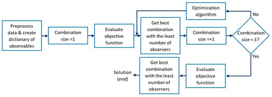
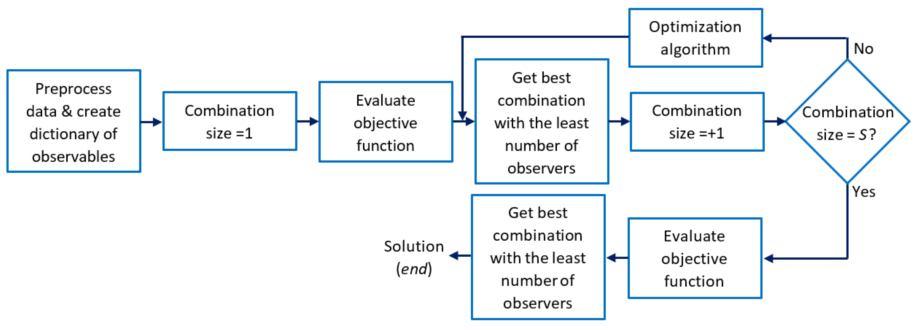
The process starts by calling the optimization algorithm with a single observable and continuing until all but one of the existing observables in the dictionary are integrated. It is important to note that each time the optimization algorithm concludes, the best combination of observables from the current call must be compared with the globally stored best combination. Finally, the objective function is called once to test the set of all observables in the dictionary, and its result is compared with the best global combination. The final outcome of the procedure will thus be the globally best combination identified and stored during the process. The explained logic is shown in Figure 1 and also in Algorithm 1.

Figure 1. A block diagram of the proposed procedure.

This methodology can be applied to any optimization algorithm. The fundamental impact of doing so, as opposed to performing an exhaustive search of the observables’ combinations, is the reduction in computational cost. One of the key factors for the success of this method is having an extensive dictionary of observables. By doing so, it is guaranteed that the user will not need expert knowledge of the system. Furthermore, for dictionaries of high dimensionality, the computational expense of an exhaustive search can become prohibitively costly.

Algorithm 1 General procedure for observable selection

1: Perform preprocessing on the data for system modeling   2: Initialize the globally best combination of observables   3: for $k=1$ to $S-1$ do   4:    Execute the optimization algorithm with k observables   5:    Retrieve the best combination of observables from the current optimization call   6:    if current combination is better than the globally best combination then   7:      Update the globally best combination   8:    end if   9: end for 10: Evaluate the objective function with all observables in the dictionary 11: if the full set of observables is better than the globally best combination then 12:    Update the globally best combination 13: end if 14: return the globally best combination of observables

3.4. Optimization Algorithms

Although deterministic optimization methods such as gradient-based methods, linear programming methods, and dynamic programming have applications across various domains, stochastic/probabilistic Methods, such as Genetic Algorithms (GA), and heuristic and metaheuristic methods like the Differential Evolution algorithm (DE) have proven to be particularly suited for the global optimization of complex, nonlinear, black-box problems in the last two decades. These intrinsic population-based algorithms are excellent for the in-depth exploration of large-sized search spaces, which results in great scalability to larger dictionary sizes. This also lends itself to inherent parallelism; hence, these types of algorithms are well adapted for high-performance computing environments where the optimization processes speed up considerably. Another relevant feature of the stochastic/probabilistic and heuristic and metaheuristic methods is that they do not depend on the differentiability or even the continuity of the objective functions, which makes them particularly well-suited for addressing irregularities or non-convexities that may arise in the identification task with data-driven methods. Because it is also possible for them to reliably converge to an optimum or near-optimum solution, they are a robust and effective tool for the identification of sparse yet accurate representations of complex dynamical systems.

The basic characteristics of GA and DE are presented below.

3.4.1. Genetic Algorithm

GA is a class of optimization algorithm inspired by the principles of natural evolution [48,49,50]. It belongs to a larger family of evolutionary algorithms and is used to solve complex optimization problems where traditional methods may fail or be inefficient. The main idea behind GA is to simulate the process of natural selection and genetic inheritance to evolve its population towards the optimal individual or solution [51].

The process begins with the random initialization of a population, where each individual represents a potential solution encoded in a specific format. The algorithm then follows an iterative cycle composed of the following key steps:

• Evaluation: Each individual is assessed by the objective function to determine its performance or quality.
• Selection: Individuals are selected probabilistically based on their objective function values. Solutions with better objective values are more likely to be chosen to contribute to the next generation, though solutions with poorer values may also be included to maintain diversity.
• Crossover (Recombination): Pairs of selected individuals undergo a recombination process to exchange genetic material. This produces offspring that combine characteristics of their parents, potentially leading to improved solutions.
• Mutation: To maintain genetic diversity and avoid premature convergence, random modifications are introduced to some individuals. This ensures that the algorithm can explore new regions of the solution space.
• Replacement: A new population is formed by replacing some or all of the previous generation with the newly generated offspring. This constitutes the next iteration of the algorithm.

The GA continues iterating through these steps until a termination criterion is met, such as reaching a maximum number of iterations or achieving a predefined objective function value. The algorithm ultimately identifies a solution that approximates the optimal value of the objective function.

The basic procedure of a single-objective GA is expressed in Algorithm 2.

Algorithm 2 Basic procedure followed by a single-objective GA

1: Initialize population with random individuals   2: Evaluate the objective function for each individual   3: Store the individual with the best objective value found so far   4: while termination condition not met do   5:    Select individuals for reproduction   6:    Apply crossover to produce offspring   7:    Apply mutation to offspring   8:    Evaluate the objective function for each offspring   9:    Update the best individual if a better one is found 10:    Select individuals to form the new population 11: end while 12: return the individual with the best objective value found

3.4.2. Differential Evolution Algorithm

DE is a population-based algorithm that searches for the global optimal solution [52] by employing GA concepts (operators) such as mutation, crossover, and selection [53].

The main steps in DE, as shown in Algorithm 3, are:

• Population initialization: A population of M individuals is randomly generated within the limits of the search space. Then, each individual is evaluated using the objective function, which assigns a value indicating the quality of each solution.
• Evolutionary cycle: To generate new individuals, the DE algorithm applies the three basic genetic operators (mutation, crossover, selection) to the entire population iteratively (see [54] for a more detailed explanation).
• Stopping criterion: The evolutionary cycle continues until at least one stopping criterion is met: reaching a maximum number of generations or having the same objective function value for a certain number of generations, among others.

Algorithm 3 Basic procedure followed by a single-objective DE

1: Initialize population with random individuals   2: Evaluate the objective function for each individual   3: Store the individual with the best objective value found so far   4: while termination condition not met do   5:    for each individual in the population do   6:      Select three distinct individuals randomly   7:      Create mutant vector by adding a weighted difference between two of them to the third   8:      Combine mutant vector with the current individual to create a trial vector   9:      Evaluate the objective function for the trial vector 10:      if trial vector has a better objective value than the individual then 11:         Replace the individual with the trial vector 12:         Update the best individual if needed 13:      end if 14:    end for 15: end while 16: return the individual with the best objective value found

3.5. Continuous Stirred Tank Reactor

In this study, a CSTR is used as a benchmark system to evaluate the performance of the proposed optimization approach. CSTRs are widely used in the chemical and process industries due to their dynamic behavior and complex nonlinear characteristics, making them ideal for testing and validating control and modeling algorithms. The primary objective of this problem is to model the reactor’s behavior using data-driven techniques and to optimize the selection of observables to improve the accuracy of the Koopman operator approximation.

The CSTR problem, presented in [55], involves a chemical process where two reactants are mixed and react to generate compound A within a mixture at temperature T. The reaction is exothermic, meaning it releases heat, which slows the reaction rate as the process progresses. To regulate the temperature and, consequently, the reaction rate, a coolant flow is introduced, allowing for control of both the temperature and concentration. This process is governed by two differential equations that describe the evolution of concentration and temperature over time:

$$\begin{array}{ccc}\hfill \dot{C_a}\left(t\right)& =& {\displaystyle \frac{q\left(t\right)}{V}}\left[C_{a0}-C_a\left(t\right)\right]-k_0{C}_a\left(t\right)exp\left[{\displaystyle \frac{-E}{RT\left(t\right)}}\right]\hfill \\ \hfill \dot{T}\left(t\right)& =& {\displaystyle \frac{q\left(t\right)}{V}}\left[T_0-T\left(t\right)\right]-{\displaystyle \frac{(-\Delta H)k_0{C}_a\left(t\right)}{\rho C_p}}\times exp\left[{\displaystyle \frac{-E}{RT\left(t\right)}}\right]\hfill \\ & & +{\displaystyle \frac{{\rho }_c{C}_{pc}}{\rho C_{p}V}}{q}_c\left(t\right)\times \left\{1-exp\left[{\displaystyle \frac{-hA}{q_c\left(t\right){\rho }_c{C}_{pc}}}\right]\right\}\left[T_{c0}-T\left(t\right)\right]\hfill \end{array}$$

(22)

The parameters, all assumed constant at nominal values, along with the thermodynamic and chemical constants involved in the reaction, are presented in Table 1.

Table 1. The CSTR Parameters.

${\mathit{C}}_{\mathit{a}}$	Product concentration	$0.1\mathrm{mol}/\mathrm{L}$
T	Reactor temperature	$438.54\mathrm{K}$
$q_c$	Coolant flow rate	$103.41\mathrm{L}{\min }^{-1}$
q	Process flow rate	$100\mathrm{L}{\min }^{-1}$
$C_{a0}$	Feed concentration	$1\mathrm{mol}/\mathrm{L}$
$T_0$	Feed temperature	$350\mathrm{K}$
$T_{c0}$	Inlet coolant temperature	$350\mathrm{K}$
V	CSTR volume	$100\mathrm{L}$
$hA$	Heat transfer coefficient	$7\times {10}^5\mathrm{cal}{\min }^{-1}{\mathrm{K}}^{-1}$
$k_0$	Reaction rate constant	$7.2\times {10}^{10}{\min }^{-\mathrm{L}}$
$E/R$	Activation energy	$1\times {10}^4\mathrm{K}$
$\Delta H$	Heat of reaction	$-2\times {10}^5\mathrm{cal}/\mathrm{mol}$
$\rho ,{\rho }_c$	Liquid densities	$1\times {10}^3\mathrm{g}/\mathrm{L}$
$C_p,C_{pc}$	Specific heats	$1\mathrm{cal}{\mathrm{g}}^{-\mathrm{L}}{\mathrm{K}}^{-1}$

For the identification procedure, a database was generated using the previous information with a white noise contamination of (2%) and a sample period of 6 s which is enough to capture all the information on the process dynamic. This database contains 7500 samples.

4. Results and Discussion

4.1. Experiments Design

Two experiments (for GA and DE, respectively) were designed, both were carried out 40 times to ensure the consistency of the results. The main characteristics of these experiments are summarized next:

• To validate the proposed methodology, a dictionary of 10 observables was defined (see Equation (23)). The used functions represent simple nonlinearities that can appear in industrial processes. The functions in the dictionary can be changed according to the requirements of the users.

  $$D=\left\{\begin{array}{c}Ob{s}_1:{(x1+x2)}^2\hfill \\ Ob{s}_2:{(x1+x2)}^3\hfill \\ Ob{s}_3:{(x1+x2)}^4/{10}^{+10}\hfill \\ Ob{s}_4:{(x1+x2)}^5/{10}^{+10}\hfill \\ Ob{s}_5:sin\left(x1\right)\hfill \\ Ob{s}_6:sin\left(x2\right)\hfill \\ Ob{s}_7:exp\left(x1\right)\hfill \\ Ob{s}_8:exp\left(x2\right)/{10}^{+200}\hfill \\ Ob{s}_9:log\left(x1\right)\hfill \\ Ob{s}_{10}:log\left(x2\right)\hfill \end{array}\right.$$

  (23)
• The 7500 samples from the database were separated into two sets: a. model estimation (6000 samples) and b. model validation (1500 samples).
• The experiments were conducted in MATLAB R2018b using a computer with the specifications shown in Table 2:
• The fundamental characteristics of the implemented GA are:

  –

  Random mechanisms are based on the default configuration of MATLAB R2018b’s “uniform pseudorandom number generator”. This may affect reproducibility in the experiments, but it also allows for a broader evaluation of the algorithm, as it will behave under different initial conditions each time a run is executed.

  –

  Population size: 50.

  –

  Selection: binary tournament.

  –

  Crossover: uniform crossover without duplicates—crossover rate: 80%.

  –

  Mutation: random mutation without duplicates—mutation rate: 2%.

  –

  Elitism: elitism with a single individual.

  –

  Stopping criteria:

  • maximum permitted error (which is associated with the calculated value of the objective function): 0;
  • maximum number of generations: 1000.

• The fundamental characteristics of the implemented DE are:

  –

  Random mechanisms are also based on the default configuration of MATLAB R2018b’s “uniform pseudorandom number generator”.

  –

  Population size: 50.

  –

  Mutation: rand/1 mutation without duplicates—mutation factor: 0.8.

  –

  Crossover: binomial crossover without duplicates—crossover factor: 0.5.

  –

  Selection: greedy selection.

  –

  Elitism: elitism with a single individual.

  –

  Stopping criteria:

  • maximum permitted error (which is associated with the calculated value of the objective function): 0;
  • maximum number of generations: 1000.

Table 2. Computer specifications.

Device specifications
Processor	Intel(R) Core(TM)2 Duo CPU E7400 @ 2.80 GHz 2.79 GHz
Installed RAM	2 GB
System type	64-bit operating system, x64-based processor
Windows specifications
Edition	Windows 10 Pro
Version	1909
OS build	18,363.418

4.2. Analysis of Results

4.2.1. Genetic Algorithm

The results after using GA as the optimization algorithm are shown in Table 3.

Table 3. GA execution results.

	Best Combination	Mean Euclidean Distance	Mean Error (${\mathit{C}}_{\mathit{a}}$)	Mean Error (T)
Results	$\left[\begin{array}{ccc}Ob{s}_1& Ob{s}_2& Ob{s}_3\\ Ob{s}_8& Ob{s}_9& Ob{s}_{10}\end{array}\right]$	$0.1083$	$8.3019\times {10}^{-4}$	$0.10826$

The selected set of observables (best combination) is:

$$D=\left\{\begin{array}{c}Ob{s}_1:{(x1+x2)}^2\hfill \\ Ob{s}_2:{(x1+x2)}^3\hfill \\ Ob{s}_3:{(x1+x2)}^4/{10}^{+10}\hfill \\ Ob{s}_8:exp\left(x2\right)/{10}^{+200}\hfill \\ Ob{s}_9:log\left(x1\right)\hfill \\ Ob{s}_{10}:log\left(x2\right)\hfill \end{array}\right.$$

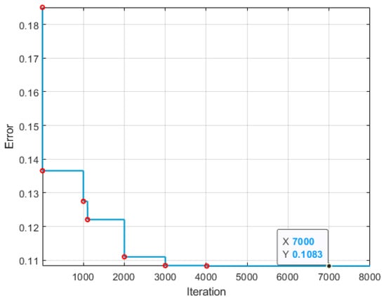
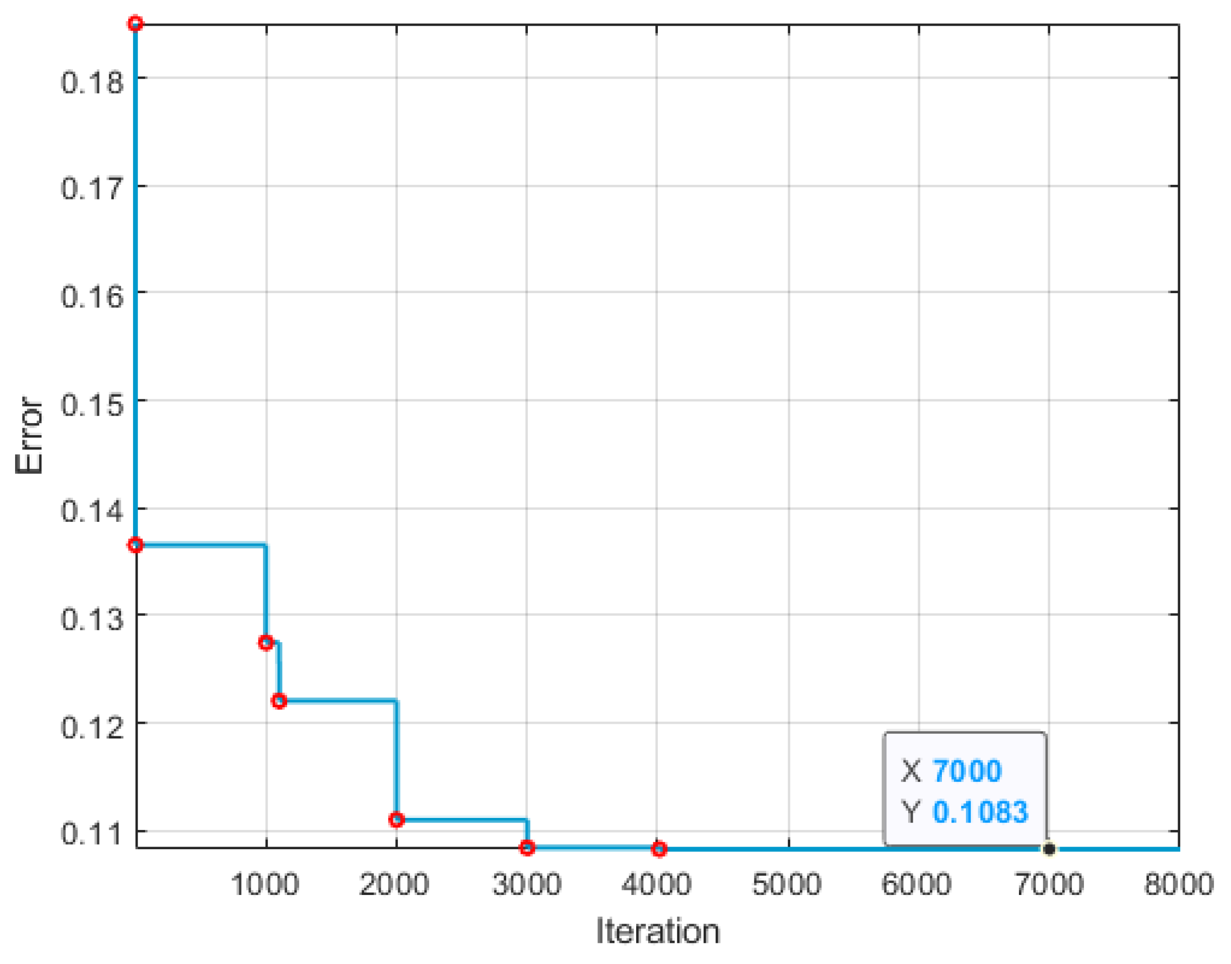
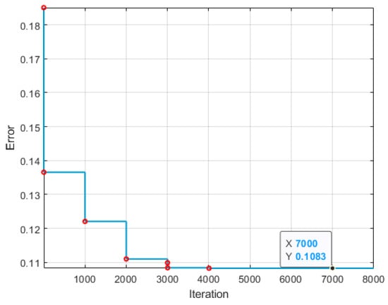
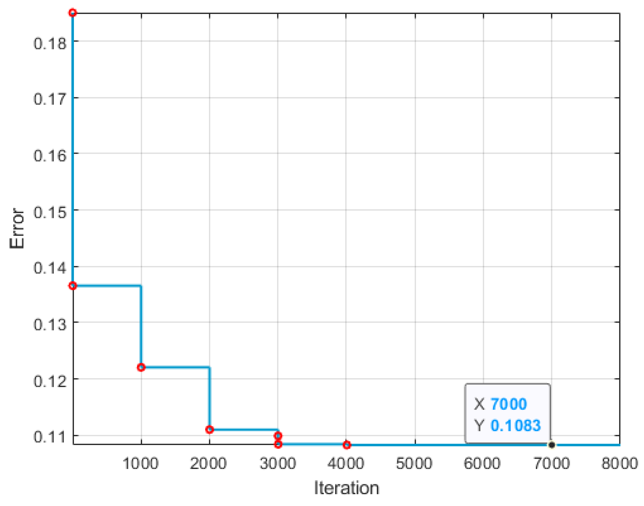
Figure 2 illustrates the evolution of the error across all generations for each GA call, along with the error for all the observables together, of one of the 40 experiments conducted. As shown, it highlights a very fast convergence toward the final solution.

Figure 2. Error (Euclidean distance) vs. iteration of the GA. Red circles indicate a change in the error value.

Equations (24)–(26) display matrices $\mathbf{A}$ and $\mathbf{B}$ for the resulting model, as well as the matrix $\Sigma$ of the eigenvalues. By examining these matrices, it can be seen that there was an increase (from 2 to 8) in the dimensionality of the system.

$$\mathbf{A}=\left[\begin{array}{cccccccc}10.453& 10.427& -0.032& 4.802e-05& -2.707e+02& 18.903& -0.043& -2.260e+02\\ -93.714& -1.545e+02& 0.581& -9.870e-04& 6.219e+03& -2.265e+03& 9.509& 2.755e+03\\ 1.517e+05& 1.191e+05& -2.804e+02& 0.297& -1.069e+06& -1.813e+06& 9.156e+03& -3.153e+06\\ 2.491e+08& 2.413e+08& -6.894e+05& 9.380e+02& -4.863e+09& -1.088e+09& 6.585e+06& -5.628e+09\\ 23.354& 23.692& -0.07& 9.840e-05& -5.280e+02& -57.377& 0.418& -5.381e+02\\ 0.001& 0.001& -3.885e-06& 5.681e-09& -0.032& 0.979& 7.796e-06& -0.028\\ -53.982& -62.174& 0.197& -2.960e-04& 1.694e+03& -22.144& -0.417& 1.329e+03\\ -0.801& -0.996& 0.003& -5.169e-06& 30.552& -5.568& 0.019& 21.262\end{array}\right]$$

(24)

$$\mathbf{B}=\left[\begin{array}{c}2.005e-04\\ -0.118\\ -1.037e+02\\ -6.849e+04\\ -0.004\\ -1.173e-08\\ 0.002\\ -2.680e-04\end{array}\right]$$

(25)

$$\Sigma =\left[\begin{array}{cccccccc}6.651e+09& 0& 0& 0& 0& 0& 0& 0\\ 0& 1.127e+05& 0& 0& 0& 0& 0& 0\\ 0& 0& 2.523& 0& 0& 0& 0& 0\\ 0& 0& 0& 0.859& 0& 0& 0& 0\\ 0& 0& 0& 0& 0.017& 0& 0& 0\\ 0& 0& 0& 0& 0& 3.236e-04& 0& 0\\ 0& 0& 0& 0& 0& 0& 2.540e-05& 0\\ 0& 0& 0& 0& 0& 0& 0& 1.266e-06\end{array}\right]$$

(26)

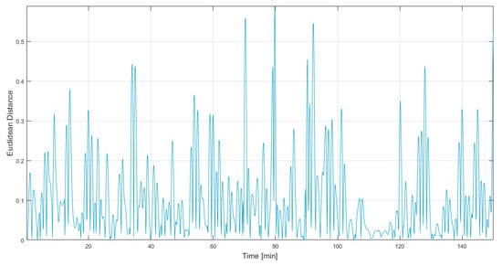
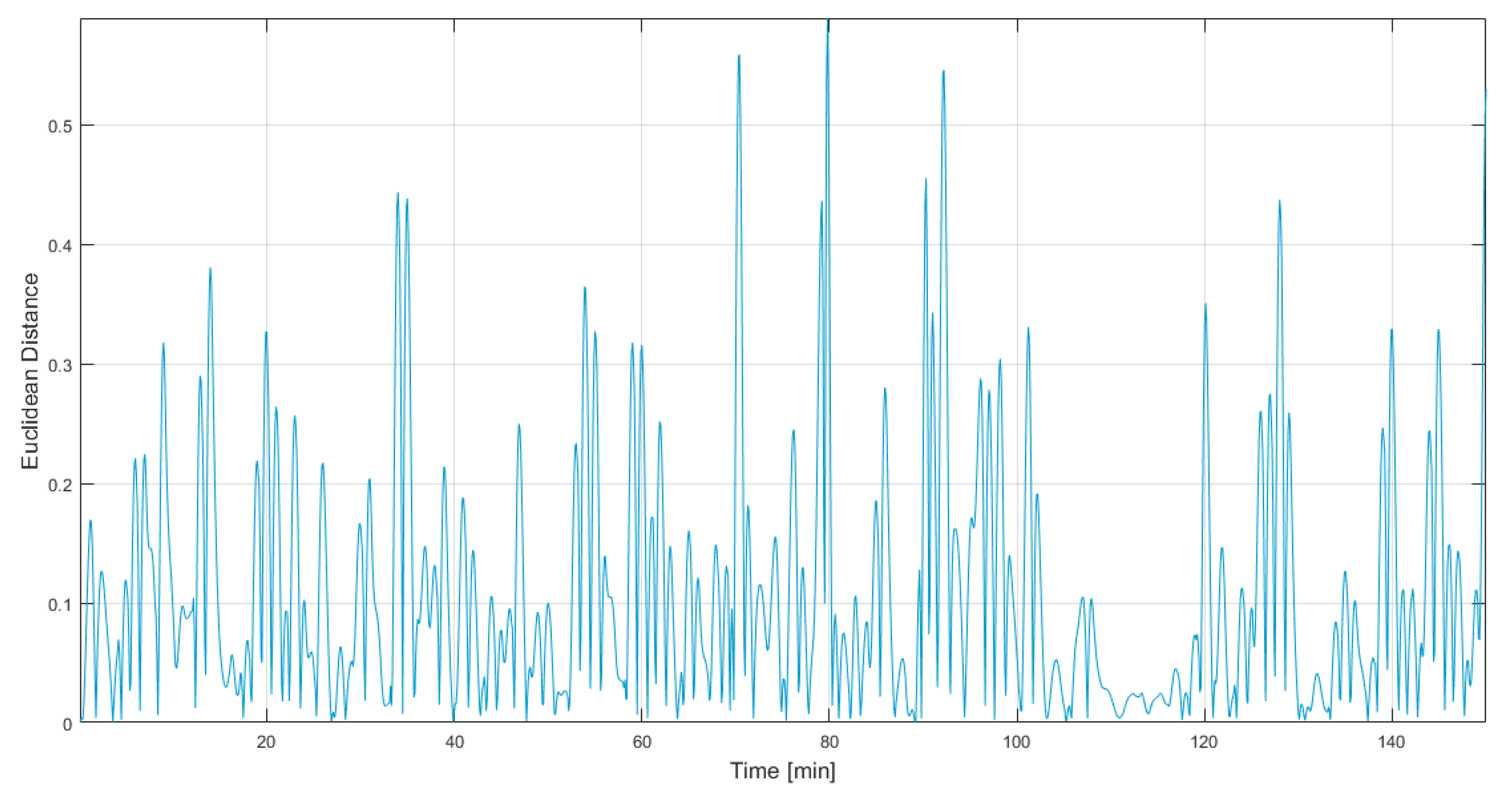
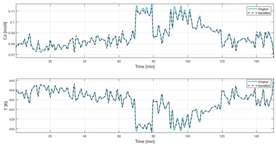
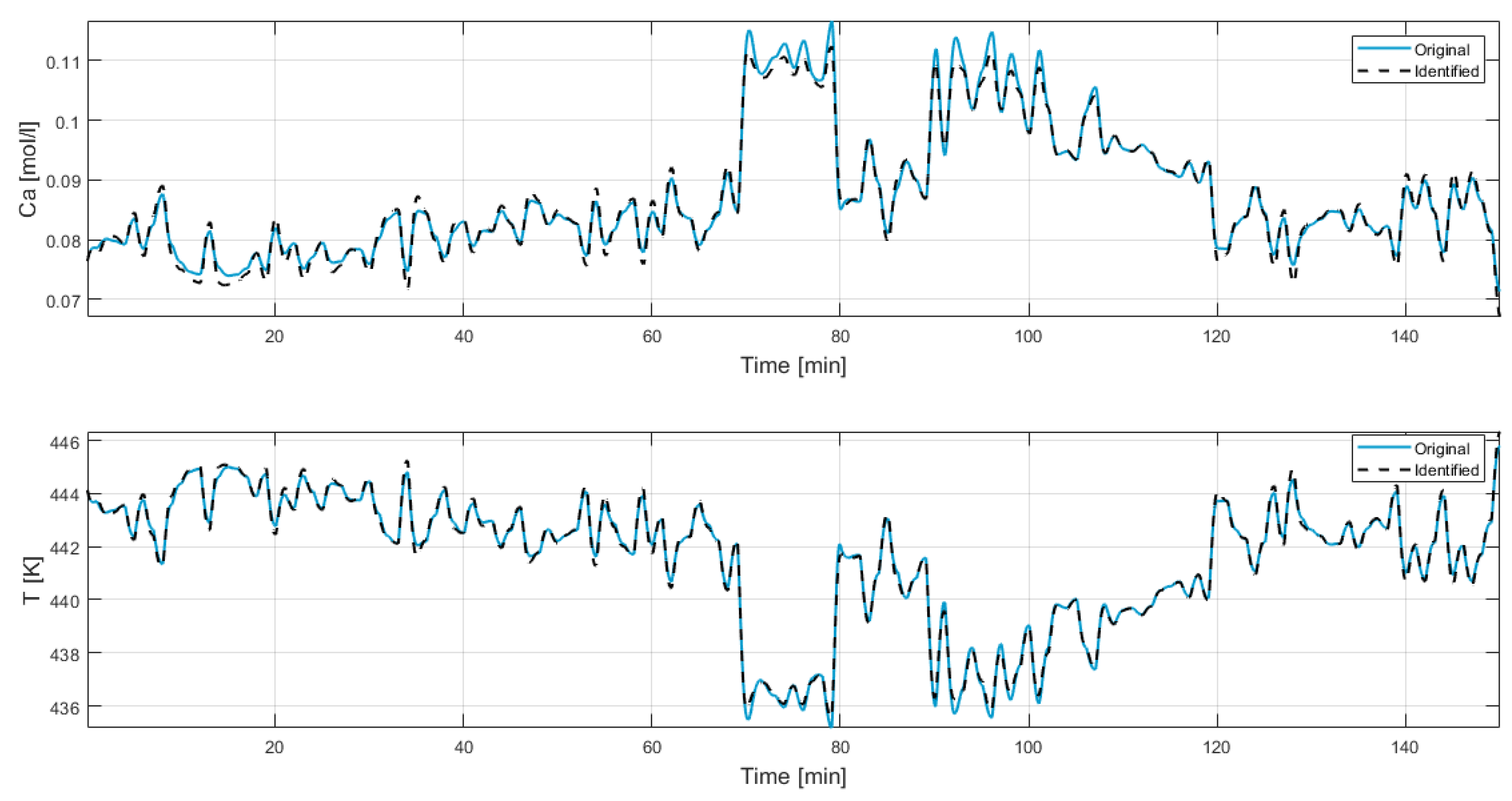
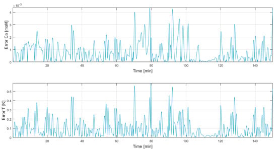
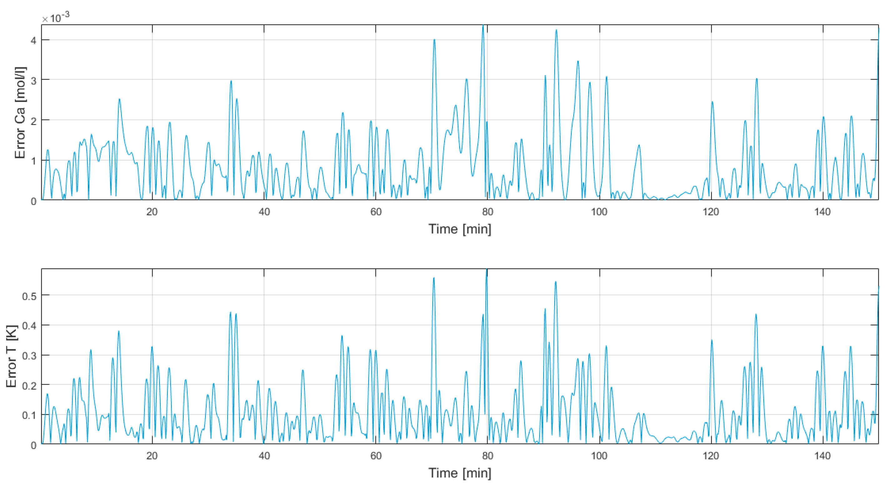
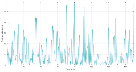
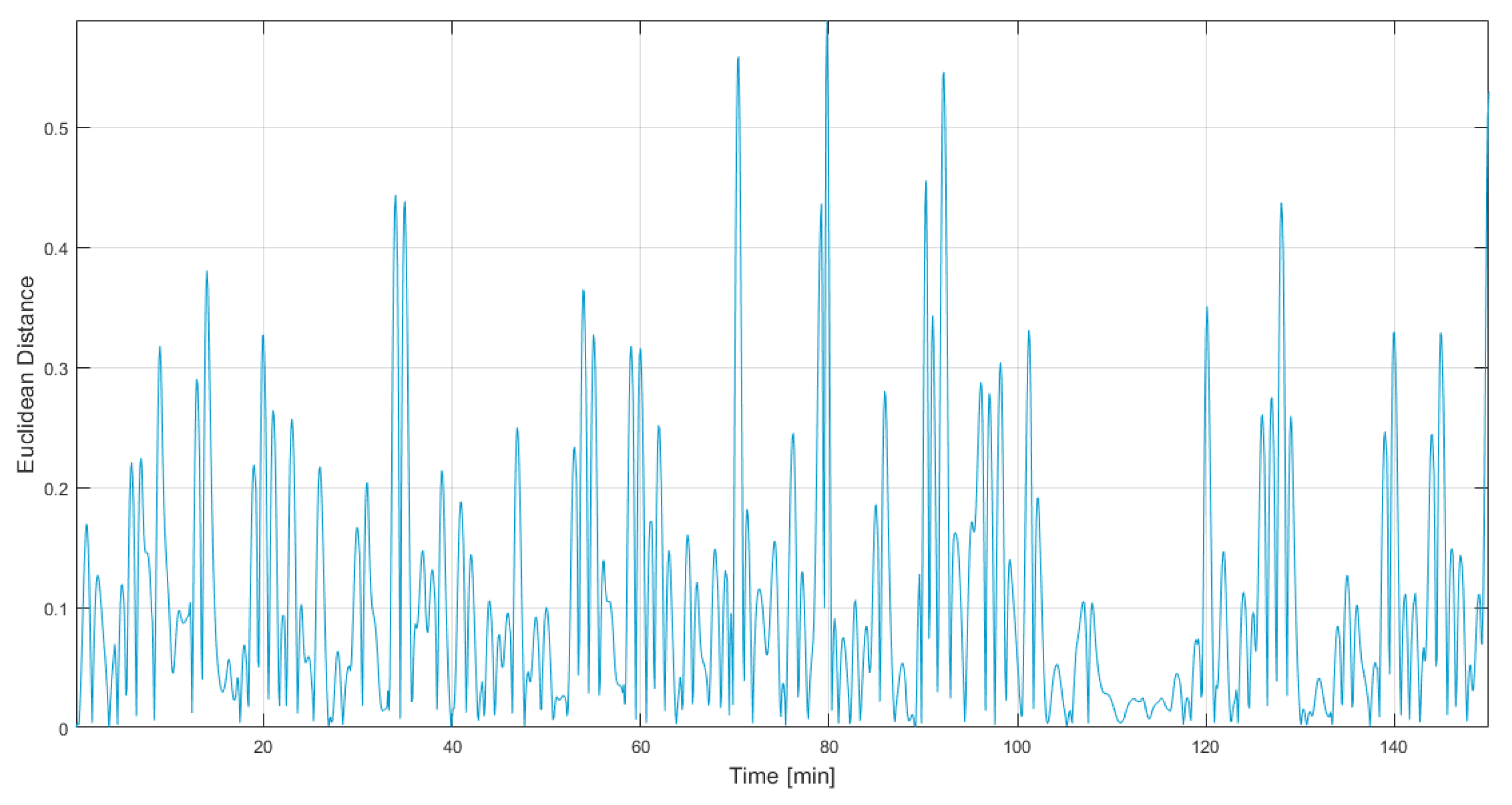
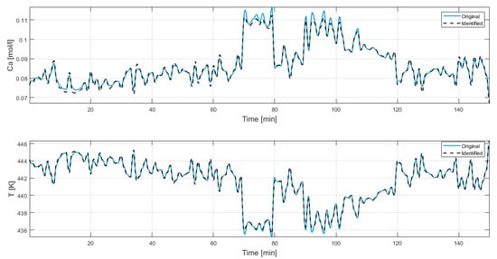
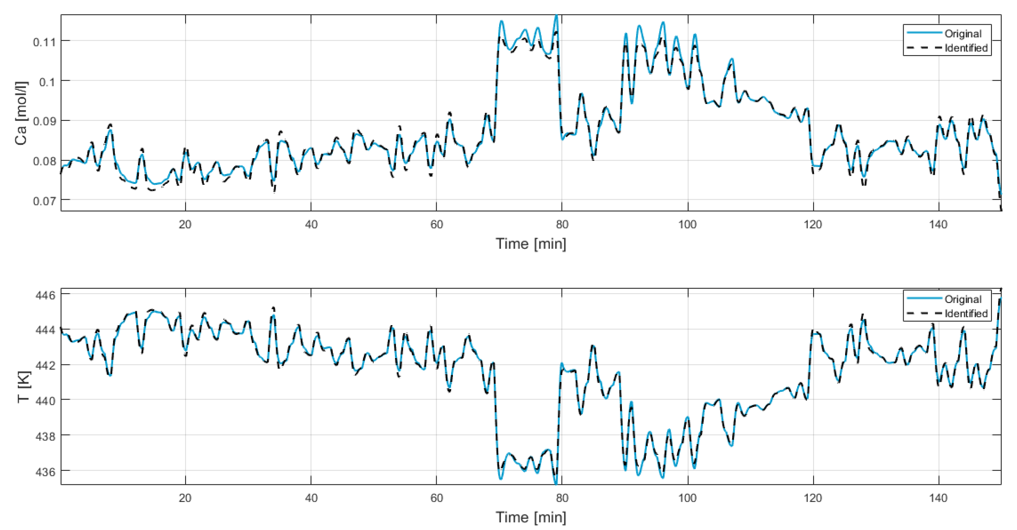
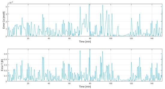
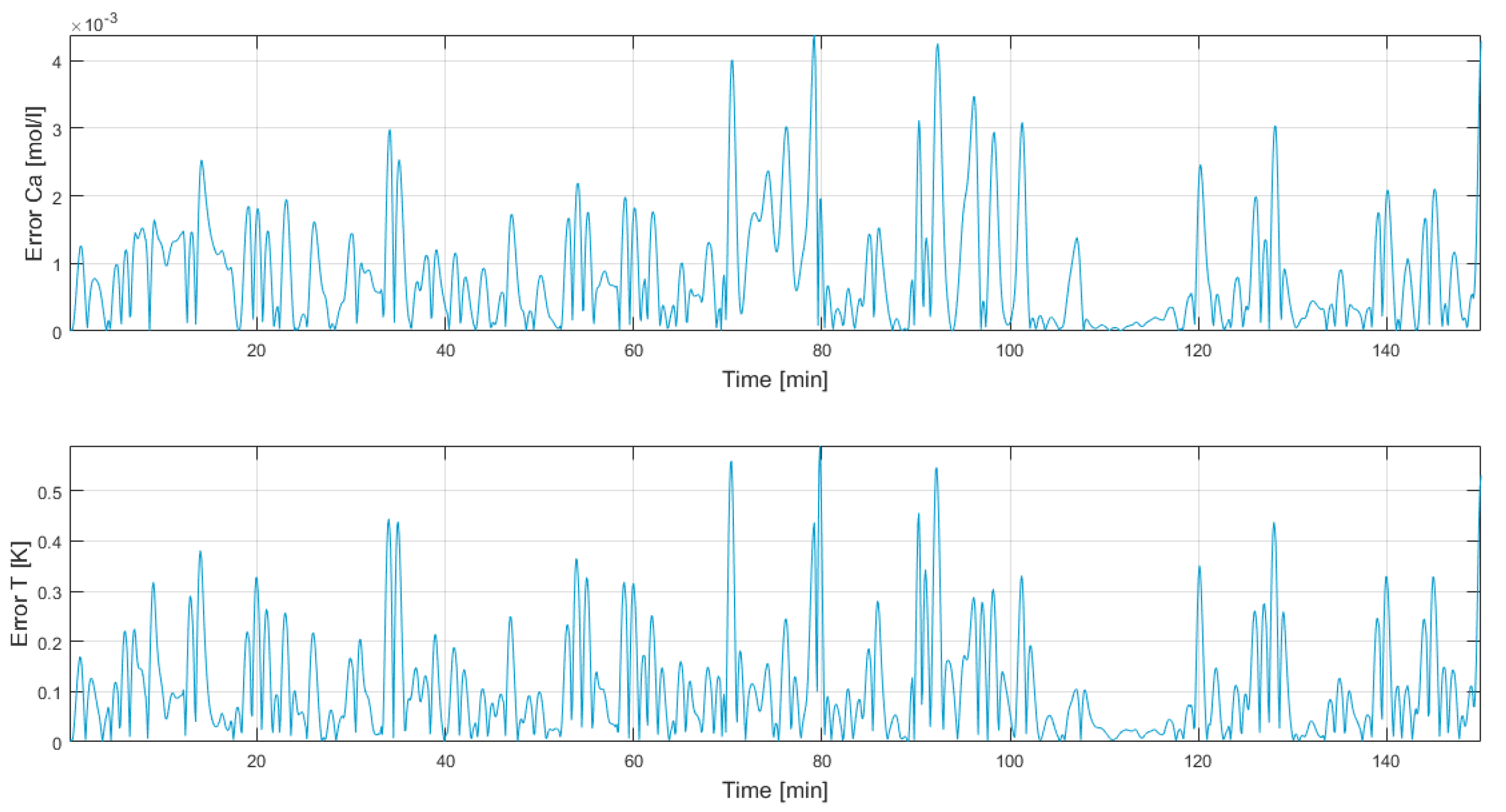
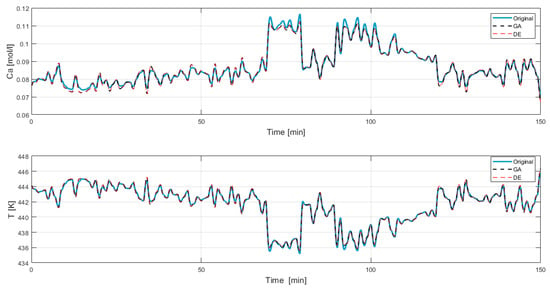
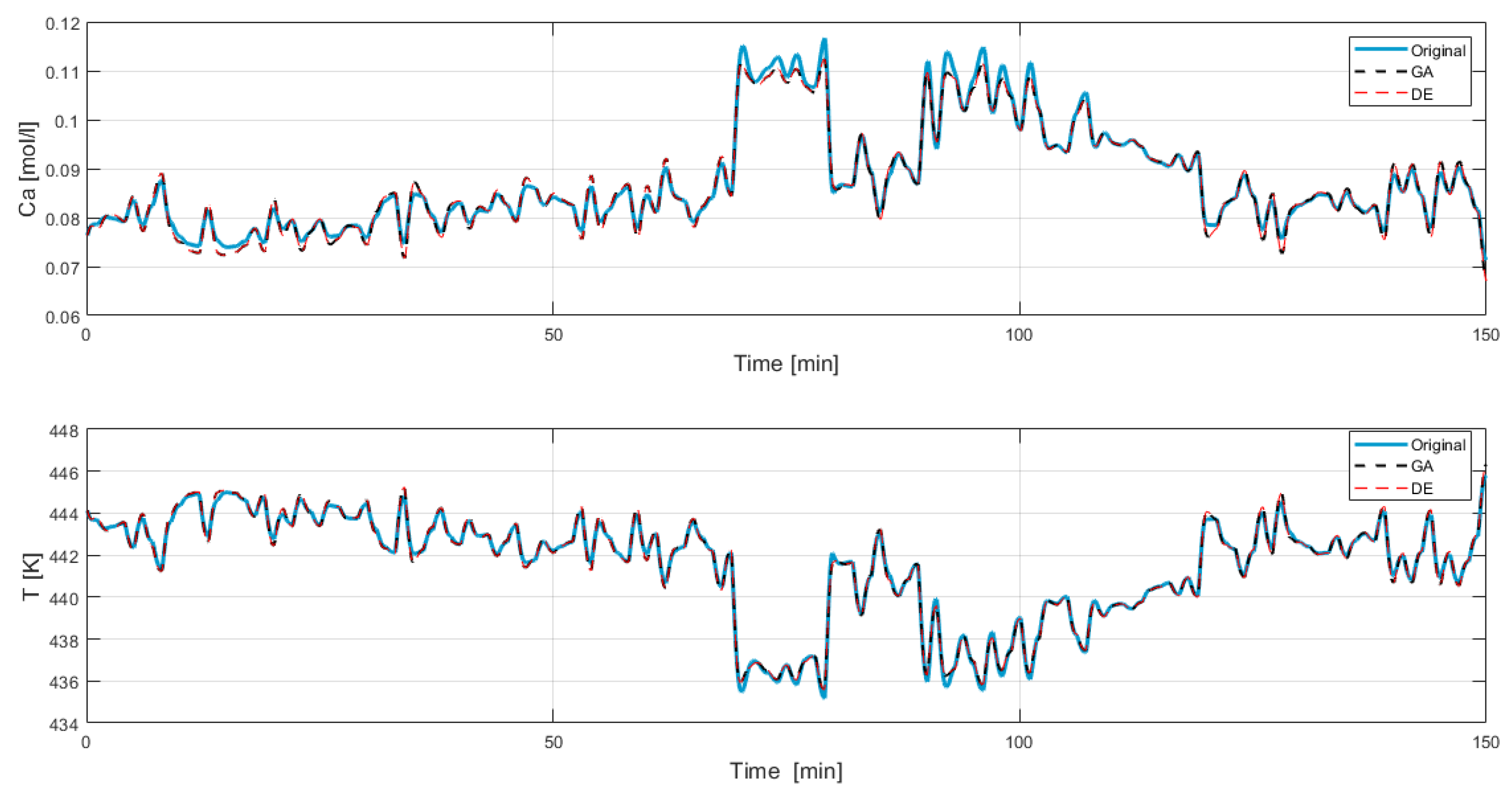
Figure 3 represents the Euclidean distance for each pair of validation points. Here, the evolution of the metric is appreciated, with the average value being the outcome of the implemented objective function. Figure 4 compares the model simulations with their corresponding measurements from the CSTR validation dataset. In this picture, it is evident that the simulated points closely follow the sampled data, although there are some discrepancies that do not seem significant. Lastly, Figure 5 depicts the absolute errors for each state-space variable. As shown, these points remain relatively small according to the variables’ working range.

Figure 3. Error between real and estimated measurements using validation data for GA.

Figure 4. Comparison between the real measurements and the simulated system response for GA.

Figure 5. Calculated system residuals for GA.

4.2.2. Differential Evolution

The DE results are shown in Table 4.

Table 4. DE execution results.

	Best Combination	Mean Euclidean Distance	Mean Error (${\mathit{C}}_{\mathit{a}}$)	Mean Error (T)
Results	$\left[\begin{array}{ccc}Ob{s}_1& Ob{s}_2& Ob{s}_3\\ Ob{s}_8& Ob{s}_9& Ob{s}_{10}\end{array}\right]$	$0.1083$	$8.3019\times {10}^{-4}$	$0.10826$

The resulting best combination is:

$$D=\left\{\begin{array}{c}Ob{s}_1:{(x1+x2)}^2\hfill \\ Ob{s}_2:{(x1+x2)}^3\hfill \\ Ob{s}_3:{(x1+x2)}^4/{10}^{+10}\hfill \\ Ob{s}_8:exp\left(x2\right)/{10}^{+200}\hfill \\ Ob{s}_9:log\left(x1\right)\hfill \\ Ob{s}_{10}:log\left(x2\right)\hfill \end{array}\right.$$

Figure 6 also illustrates the evolution of the error, which also highlights a fast convergence toward the final solution.

Figure 6. Error (Euclidean distance) vs. iteration of the DE. Red circles indicate a change in the error value.

Matrices $\mathbf{A}$, $\mathbf{B}$ and $\Sigma$ are shown in Equations (27)–(29). Here, the increased dimensionality of the system is also highlighted.

$$\mathbf{A}=\left[\begin{array}{cccccccc}10.453& 10.427& -0.032& 4.802e-05& -2.707e+02& 18.903& -0.043& -2.260e+02\\ -93.714& -1.545e+02& 0.581& -9.870e-04& 6.219e+03& -2.265e+03& 9.509& 2.755e+03\\ 1.517e+05& 1.191e+05& -2.804e+02& 0.297& -1.069e+06& -1.813e+06& 9.156e+03& -3.153e+06\\ 2.491e+08& 2.413e+08& -6.894e+05& 9.380e+02& -4.863e+09& -1.088e+09& 6.585e+06& -5.628e+09\\ 23.354& 23.692& -0.07& 9.840e-05& -5.280e+02& -57.377& 0.418& -5.381e+02\\ 0.001& 0.001& -3.885e-06& 5.681e-09& -0.032& 0.979& 7.796e-06& -0.028\\ -53.982& -62.174& 0.197& -2.960e-04& 1.694e+03& -22.144& -0.417& 1.329e+03\\ -0.801& -0.996& 0.003& -5.169e-06& 30.552& -5.568& 0.019& 21.262\end{array}\right]$$

(27)

$$\mathbf{B}=\left[\begin{array}{c}2.005e-04\\ -0.118\\ -1.037e+02\\ -6.849e+04\\ -0.004\\ -1.173e-08\\ 0.002\\ -2.680e-04\end{array}\right]$$

(28)

$$\Sigma =\left[\begin{array}{cccccccc}6.651e+09& 0& 0& 0& 0& 0& 0& 0\\ 0& 1.127e+05& 0& 0& 0& 0& 0& 0\\ 0& 0& 2.523& 0& 0& 0& 0& 0\\ 0& 0& 0& 0.859& 0& 0& 0& 0\\ 0& 0& 0& 0& 0.017& 0& 0& 0\\ 0& 0& 0& 0& 0& 3.236e-04& 0& 0\\ 0& 0& 0& 0& 0& 0& 2.540e-05& 0\\ 0& 0& 0& 0& 0& 0& 0& 1.266e-06\end{array}\right]$$

(29)

Finally, Figure 7, Figure 8 and Figure 9 display the simulation results. Since the final results of both optimization algorithms are the same, the images of the results are identical to those previously displayed. Therefore, DE also achieves satisfactory results.

Figure 7. Error between the real and estimated measurements using validation data for DE.

Figure 8. Comparison between the real measurements and the simulated system response for DE.

Figure 9. Calculated system residuals for DE.

4.2.3. Comparison Between the Optimization Algorithms

The results, presented above and in Figure 10, demonstrate that both GA and DE converged to the same optimal solution, identifying the set of observables that minimize the error. These results were validated after an exhaustive test in which all possible combinations of observables were used, derived from the 11 subsets of observables that can be formed (including the null set of observables). This outcome underscores the robustness of both algorithms, as they consistently found the best solution, indicating their suitability for this type of optimization problem. Moreover, the optimal set of observables achieved an excellent model fit, as shown in the cross-validation plot. The comparison between the model predictions and the actual process data reveals a close alignment, suggesting that the resulting model accurately captures the essential dynamics of the system under study. These findings highlight the effectiveness of evolutionary algorithms in automatically selecting Koopman observables for data-driven modeling, validating the proposed approach in this work.

Figure 10. A comparison between the real measurements and the simulated system response for GA and DE.

The objective of this work is not to compare the implemented algorithms. Conversely, the idea is to demonstrate that any optimization algorithm can be valid for the methodology. However, in order to maintain the quality of the study, we present some comparative metrics in Table 5.

Table 5. An analysis of the computational cost per optimization algorithm.

Case	Average Execution Time (min)	Average Time per Call to Optimization Algorithm (min)	Average of Objective Function Calls
GA	53.2	6.64	39,665
DE	54.8	6.85	39,915

The resulting $\Sigma$ Equation (26) reveals that the singular values in the last three rows are significantly small, indicating the presence of three dynamics that contribute minimally to the model’s accuracy. Based on this observation, future research will focus on improving the selection process of Koopman observables by incorporating a weighting mechanism. This mechanism will prioritize individuals with smaller sets of observables, ensuring that the reduction in the error remains comparable to that achieved by the individual with the lowest error, while preserving the model’s overall performance.

5. Architecture Proposal for a Practical Implementation in Industrial Environments

The IoT plays a crucial role in gathering ample data for analysis within a system [56], while digital twins enable remote monitoring, support, and maintenance tasks. Additionally, the Open-Platform Communications Unified Architecture (OPC UA) [57], the most widely used data connectivity standard in Industry 4.0, offers a service-oriented architecture. This allows for smooth communication between controllers, sensors, actuators, devices, applications, and server-based systems without the need for custom drivers for data exchange [58].

Industry 4.0 refers to the integration of smart computing and networking technologies into industrial production and manufacturing processes for automation, reliability, and control. This integration fosters the development of the IIoT. The growing adoption of IoT applications in industry and the success of Cloud Computing services have fueled the emergence of a new computing model: Edge Computing, which processes data at the network’s edge [59].

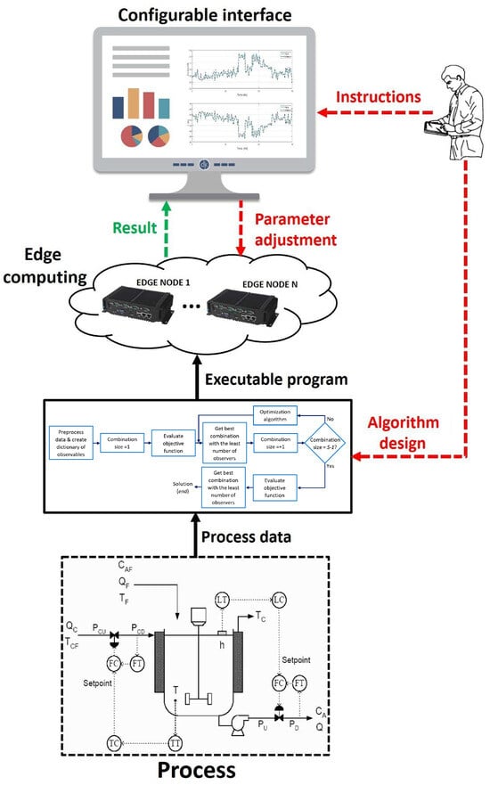
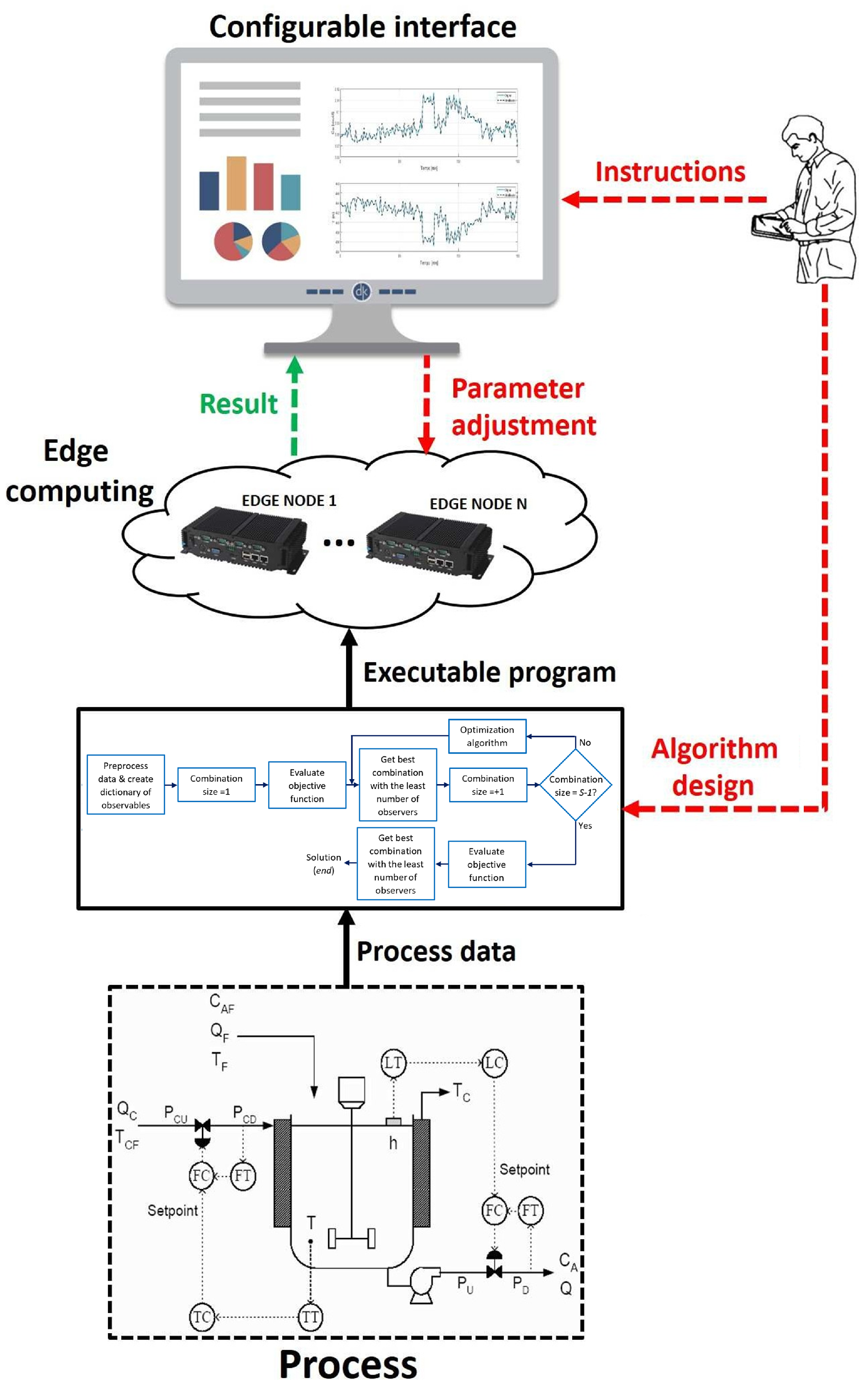
The adoption of Edge Computing nodes provides significant benefits for the practical deployment of digital twin-based systems [60]. As illustrated in Figure 11, the methodology described in this paper can be effectively implemented in an industrial environment through Edge Computing. This technology improves performance by reducing latency, optimizing bandwidth usage, and enhancing data security and privacy. Furthermore, it supports the goals of efficient management, effective resource utilization, and timely maintenance.

Figure 11. Overall diagram for proposed methodology in an IIoT system using Edge Computing.

In Edge Computing, devices not only consume data but also generate it. At the edge, these devices can request services and data from the cloud while also performing tasks traditionally handled by the cloud. Additionally, edge devices can cache, process, and manage the distribution of requests and services from the cloud to the end user.

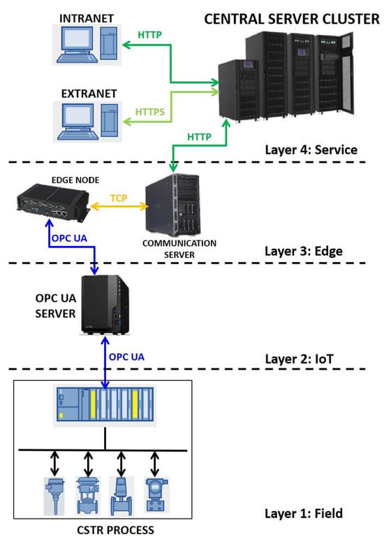
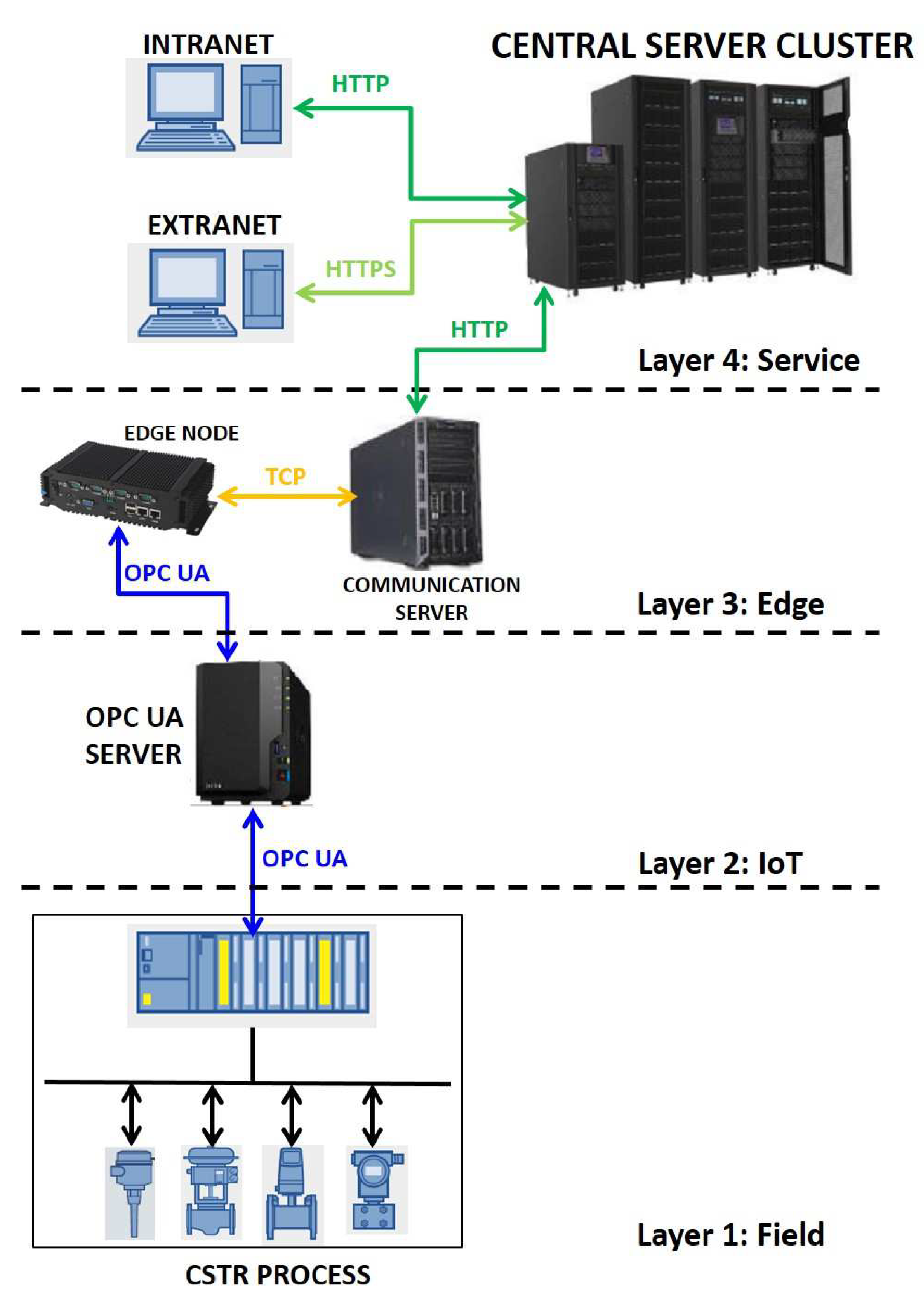
The methodology outlined in this paper can be implemented using a four-layer architecture (see Figure 12), similar to the one proposed in [60]: the field, IoT, edge, and service layers. Table 6 provides a summary of the primary functions associated with each layer.

Figure 12. Four-layer system architecture.

Table 6. Principal functions supplied by the four layers.

Layer	Function	Information
1: Field	Device deployment	Located at the base of the architecture, it includes various IoT devices like sensors, actuators, and controllers that allow for measurements of the process and control over it. The Programmable Logic Controllers (PLCs) are connected to the production equipment and supply real-time condition data utilizing diverse protocols such as OPC UA.
2: IoT	Access to process data	IoT services are taken advantage of to improve the efficiency of field devices in production using different communication protocols (Example: OPC UA).
3: Edge	Algorithm running Data communication	Include both the Edge Computing nodes and the communication server. The edge nodes function as end-points and execute the monitoring algorithms. By utilizing different network ports, multiple algorithms can run simultaneously. They also act as a link between the frontend interface and the remote monitoring system.
4: Service	Algorithm design Web service	This is utilized to offer a range of services, such as web access, algorithm design, data storage, and analysis service. Both intranet and extranet users can access the web after authentication.

A Proposal for Design and Implementation

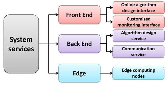
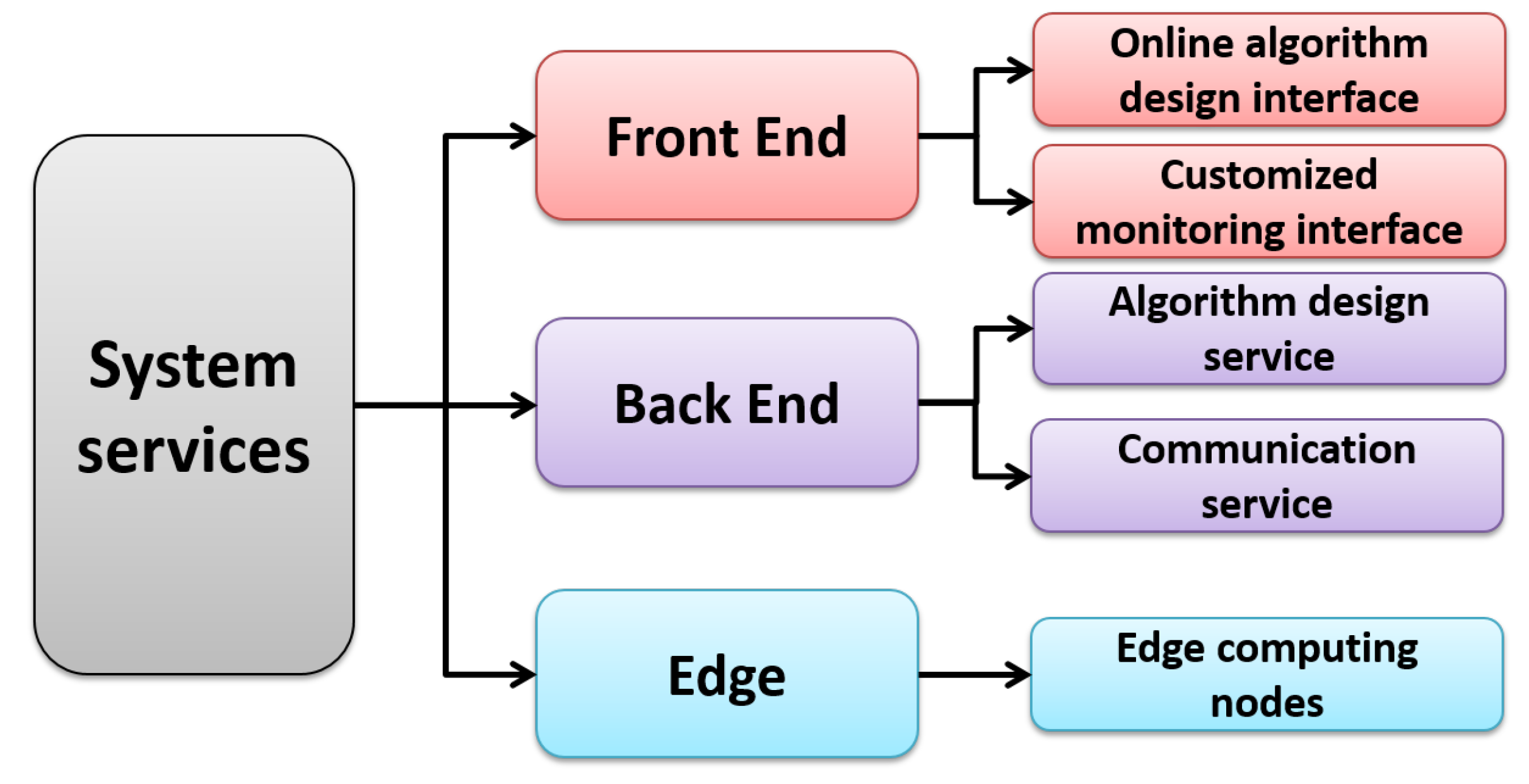
Based on the four-tier architecture, it is possible to implement several services in the system. As Figure 13 shows, these services are designed between the front end, back end, and edge.

Figure 13. Main services provided by front end, back end, and edge.

The front end is responsible for the representation of the design interface of the proposed methodology and the monitoring interface. For implementing the proposed method, users can build the algorithm diagram online from the design interface. Currently, the front-end developers use frameworks such as AngularJS, Vue.JS, jQuery, EmberJS or Svelte, among others, for interface design. These frameworks allow them to write and organize the application in an efficient way. Subsequently, the diagram of the proposed methodology should be converted into JSON (JavaScript Object Notation) data to then generate the executable program. The JSON data contains detailed information about the design methodology, including simulation/compilation configurations.

On the other hand, the back end provides the data, logic and communication for the front end. Multiple open-source softwares can be used to provide the back-end services, including Nginx, C#, Ruby, MySQL, and FFmpeg, to name just a few. In addition, an algorithm design server can be implemented that allows users to convert the diagram of the methodology designed in the front end into an online executable program.

Meanwhile, edge nodes provide Edge Computing services for algorithm execution. In this proposal, the designed methodology can be executed on the remote edge nodes when the users download the algorithm on the interface. The algorithm running on these nodes receives and processes the data in real-time. Afterward, the results of the algorithm execution are returned to the communication server to be displayed on the interface.

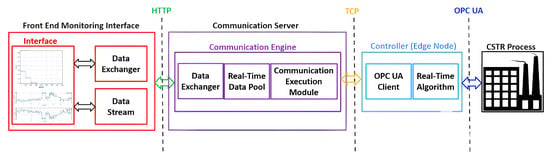
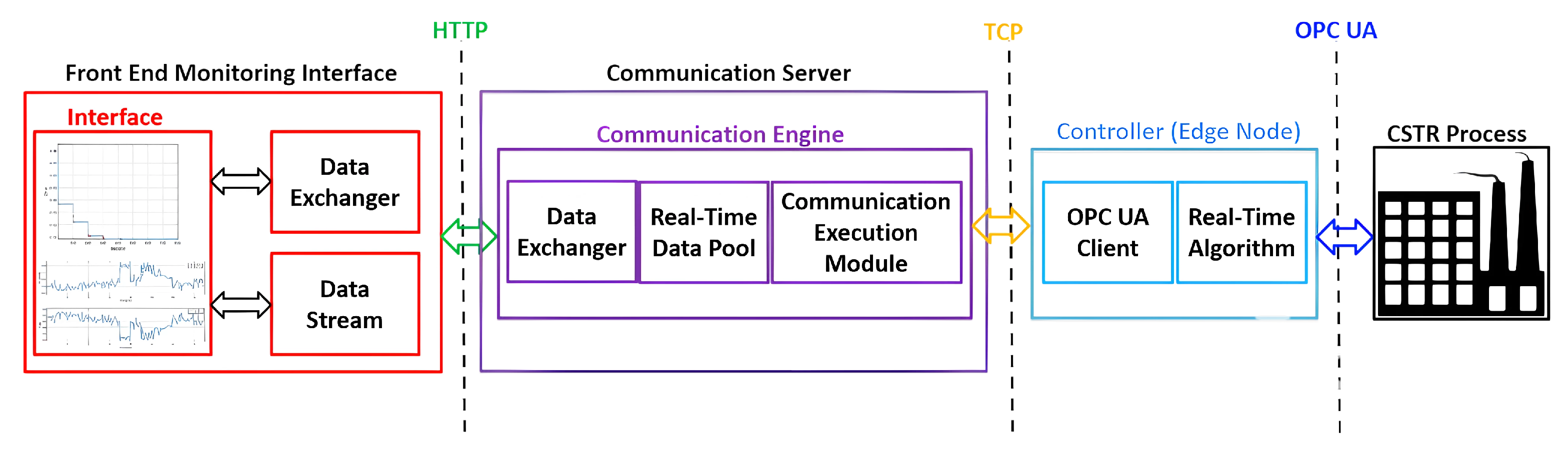
Figure 14 shows the data communication channels that should be designed for the proposed approach. For this process, there is a communication engine, which should be implemented in the communication server. The communication execution module functions as an the interface to the process. A Transmission Control Protocol (TCP) connection should be established between the communication execution module and the OPC UA client program when the algorithm is downloaded and running on the edge node. The real-time condition data obtained using the OPC UA protocol are temporarily stored in a real-time data pool.

Figure 14. Communication channels between front end, back end, and edge.

An HTTP communication channel between the widgets in the monitoring interface and the corresponding data exchanger must be created once a user starts the monitoring process successfully. First, the latest packaged data from the real-time data pool are transmitted to the front-end interface, which synchronizes the widgets configured in the monitoring interface. In addition, user instructions and parameters settings can be processed through this communication channel.

6. Conclusions

This work has demonstrated the effectiveness of an optimization-based algorithm for automatically selecting Koopman observables in the context of DMDc for digital twin development. By leveraging DMDc, the matrices $\mathbf{A}$ and $\mathbf{B}$ of the discrete linear system were obtained directly from process observations, offering a structured framework compatible with classical control theory. This approach enhances the usability of data-driven models for real-time analysis, prediction, and control.

A key outcome of this study is the ability to identify nonlinear dynamics without requiring expert knowledge of the system. The optimization algorithm ensures that the best combinations of observables are selected, thus providing an automated alternative to traditional expert-driven methods. This represents a significant advancement in bridging data-based modeling and classical control theory, enabling industries to more easily deploy digital twins in complex systems. Furthermore, when the method determines the smallest set of observable functions that best approximate the real process, experts will have a set of functions that best describe the nonlinearities of the system, providing valuable support for addressing a deeper study of it.

The results validate the proposed methodology’s capacity to accurately model nonlinear systems while maintaining computational efficiency. Additionally, the importance of a broad dictionary of observables was emphasized to ensure coverage of diverse types of nonlinearities. Ensuring the quality and quantity of data samples is also highlighted as a critical factor for capturing the fundamental dynamics of the system.

The following issues will be addressed in future studies:

• The improvement of the selection process of Koopman observables by incorporating a weighting mechanism. The idea is to prioritize individuals with smaller sets of observables while preserving the model’s overall performance.
• The selection of an optimization technique that would provide the best results in terms of convergence, computational complexity, and other indicators for evaluating the method’s efficiency.

References

- Tran, M.Q.; Doan, H.P.; Vu, V.Q.; Vu, L.T. Machine learning and IoT-based approach for tool condition monitoring: A review and future prospects. Measurement 2023, 207, 112351. [Google Scholar] [CrossRef] [Scilit]
- Surucu, O.; Gadsden, S.A.; Yawney, J. Condition Monitoring using Machine Learning: A Review of Theory, Applications, and Recent Advances. Expert Syst. Appl. 2023, 221, 119738. [Google Scholar] [CrossRef] [Scilit]
- Achouch, M.; Dimitrova, M.; Ziane, K.; Sattarpanah Karganroudi, S.; Dhouib, R.; Ibrahim, H.; Adda, M. On Predictive Maintenance in Industry 4.0: Overview, Models, and Challenges. Appl. Sci. 2022, 12, 8081. [Google Scholar] [CrossRef] [Scilit]
- Margherita, E.G.; Braccini, A.M. Industry 4.0 Technologies in Flexible Manufacturing for Sustainable Organizational Value: Reflections from a Multiple Case Study of Italian Manufacturers. Inf. Syst. Front. 2023, 25, 995–1016. [Google Scholar] [CrossRef] [Scilit]
- El-Kady, A.H.; Halim, S.; El-Halwagi, M.M.; Khan, F. Analysis of safety and security challenges and opportunities related to cyber-physical systems. Process Saf. Environ. Prot. 2023, 173, 384–413. [Google Scholar] [CrossRef] [Scilit]
- Xu, Z.; Elomri, A.; Baldacci, R.; Kerbache, L.; Wu, Z. Frontiers and trends of supply chain optimization in the age of industry 4.0: An operations research perspective. Ann. Oper. Res. 2024, 338, 1359–1401. [Google Scholar] [CrossRef] [Scilit]
- Barata, J.; Cardoso, J.C.S.; Cunha, P.R. Mass customization and mass personalization meet at the crossroads of Industry 4.0: A case of augmented digital engineering. Syst. Eng. 2023, 26, 715–727. [Google Scholar] [CrossRef] [Scilit]
- Han, B.; Habibi, M.A.; Richerzhagen, B.; Schindhelm, K.; Zeiger, F.; Lamberti, F.; Pratticò, F.G.; Upadhya, K.; Korovesis, C.; Belikaidis, I.P.; et al. Digital Twins for Industry 4.0 in the 6G Era. IEEE Open J. Veh. Technol. 2023, 4, 820–835. [Google Scholar] [CrossRef] [Scilit]
- Knebel, F.; Trevisan, R.; Nascimento, G.; Abel, M.; Wickboldt, J. A study on cloud and edge computing for the implementation of digital twins in the Oil & Gas industries. Comput. Ind. Eng. 2023, 182, 109363. [Google Scholar] [CrossRef] [Scilit]
- Muthuswamy, P.; Shunmugesh, K. Artificial intelligence-based tool condition monitoring for digital twins and industry 4.0 applications. Int. J. Interact. Des. Manuf. (IJIDeM) 2023, 17, 1067–1087. [Google Scholar] [CrossRef] [Scilit]
- Stadtmann, F.; Rasheed, A.; Kvamsdal, T.; Johannessen, K.A.; San, O.; Kölle, K.; Tande, J.O.; Barstad, I.; Benhamou, A.; Brathaug, T.; et al. Digital Twins in Wind Energy: Emerging Technologies and Industry-Informed Future Directions. IEEE Access 2023, 11, 110762–110795. [Google Scholar] [CrossRef] [Scilit]
- Tepljakov, A. Intelligent Control and Digital Twins for Industry 4.0. Sensors 2023, 23, 4036. [Google Scholar] [CrossRef] [Scilit]
- Semeraro, C.; Aljaghoub, H.; Abdelkareem, M.A.; Alami, A.H.; Olabi, A. Digital twin in battery energy storage systems: Trends and gaps detection through association rule mining. Energy 2023, 273, 127086. [Google Scholar] [CrossRef] [Scilit]
- Maschler, B.; Weyrich, M. Deep Transfer Learning for Industrial Automation: A Review and Discussion of New Techniques for Data-Driven Machine Learning. IEEE Ind. Electron. Mag. 2021, 15, 65–75. [Google Scholar] [CrossRef] [Scilit]
- Bruder, D.; Fu, X.; Gillespie, R.B.; Remy, C.D.; Vasudevan, R. Data-Driven Control of Soft Robots Using Koopman Operator Theory. IEEE Trans. Robot. 2021, 37, 948–961. [Google Scholar] [CrossRef] [Scilit]
- Ren, K.; Liu, J.; Wu, Z.; Liu, X.; Nie, Y.; Xu, H. A data-driven DRL-based home energy management system optimization framework considering uncertain household parameters. Appl. Energy 2024, 355, 122258. [Google Scholar] [CrossRef] [Scilit]
- Ruiz-Sarmiento, J.R.; Monroy, J.; Moreno, F.A.; Galindo, C.; Bonelo, J.M.; Gonzalez-Jimenez, J. A predictive model for the maintenance of industrial machinery in the context of industry 4.0. Eng. Appl. Artif. Intell. 2020, 87, 103289. [Google Scholar] [CrossRef] [Scilit]
- Kutz, J.N.; Brunton, S.L.; Brunton, B.W.; Proctor, J.L. Dynamic Mode Decomposition: Data-Driven Modeling of Complex Systems; SIAM: Philadelphia, PA, USA, 2016. [Google Scholar]
- Shi, L.; Liu, Z.; Karydis, K. Koopman Operators for Modeling and Control of Soft Robotics. Curr. Robot. Rep. 2023, 4, 23–31. [Google Scholar] [CrossRef] [Scilit]
- Manzoor, W.A.; Rawashdeh, S.; Mohammadi, A. Vehicular Applications of Koopman Operator Theory—A Survey. IEEE Access 2023, 11, 25917–25931. [Google Scholar] [CrossRef] [Scilit]
- Rahmani, M.; Redkar, S. Data-driven Koopman fractional order PID control of a MEMS gyroscope using bat algorithm. Neural Comput. Appl. 2023, 35, 9831–9840. [Google Scholar] [CrossRef] [Scilit]
- Swaminathan, B.; Manathara, J.G.; Vinayagam, A.K. Application of Dynamic Mode Decomposition with Control (DMDc) for aircraft parameter estimation. IFAC-PapersOnLine 2022, 55, 789–794. [Google Scholar] [CrossRef] [Scilit]
- Bai, Z.; Kaiser, E.; Proctor, J.L.; Kutz, J.N.; Brunton, S.L. Dynamic Mode Decomposition for Compressive System Identification. AIAA J. 2020, 58, 561–574. [Google Scholar] [CrossRef] [Scilit]
- Sunny, K.; Sheikh, A.; Wagh, S. Application of Dynamic Mode Decomposition for Temperature Analysis in Smart Building. In Proceedings of the 2020 7th International Conference on Control, Decision and Information Technologies (CoDIT), Prague, Czech Republic, 29 June–2 July 2020; Volume 1, pp. 1197–1202. [Google Scholar] [CrossRef] [Scilit]
- Proctor, J.L.; Brunton, S.L.; Kutz, J.N. Dynamic mode decomposition with control. SIAM J. Appl. Dyn. Syst. 2016, 15, 142–161. [Google Scholar] [CrossRef] [Scilit]
- Williams, M.O.; Kevrekidis, I.G.; Rowley, C.W. A data-driven approximation of the Koopman operator: Extending dynamic mode decomposition. J. Nonlinear Sci. 2015, 25, 1307–1346. [Google Scholar] [CrossRef] [Scilit]
- Colbrook, M.J.; Li, Q.; Raut, R.V.; Townsend, A. Beyond expectations: Residual dynamic mode decomposition and variance for stochastic dynamical systems. Nonlinear Dyn. 2024, 112, 2037–2061. [Google Scholar] [CrossRef] [Scilit]
- Garmaev, S.; Fink, O. Deep Koopman Operator-based degradation modelling. Reliab. Eng. Syst. Saf. 2024, 251, 110351. [Google Scholar] [CrossRef] [Scilit]
- Nozawa, I.; Kamienski, E.; O’Neill, C.; Asada, H.H. A Monte Carlo Approach to Koopman Direct Encoding and Its Application to the Learning of Neural-Network Observables. IEEE Robot. Autom. Lett. 2024, 9, 2264–2271. [Google Scholar] [CrossRef] [Scilit]
- Philipp, F.M.; Schaller, M.; Worthmann, K.; Peitz, S.; Nüske, F. Error bounds for kernel-based approximations of the Koopman operator. Appl. Comput. Harmon. Anal. 2024, 71, 101657. [Google Scholar] [CrossRef] [Scilit]
- Bandtlow, O.F.; Just, W.; Slipantschuk, J. EDMD for expanding circle maps and their complex perturbations. Appl. Comput. Harmon. Anal. 2024, 73, 101690. [Google Scholar] [CrossRef] [Scilit]
- Hasebe, T.; Uchiyama, K.; Masuda, K. Multilayer Extended Dynamic Mode Decomposition for Coupled Van der Pol Oscillators. In Proceedings of the 2024 28th International Conference on Methods and Models in Automation and Robotics (MMAR), Virtual, 27–30 August 2024; pp. 352–357. [Google Scholar] [CrossRef] [Scilit]
- Kar, A.K.; Akhter, M.M.; Mishra, A.C.; Mohanty, S.K. EDMD: An Entropy based Dissimilarity measure to cluster Mixed-categorical Data. Pattern Recognit. 2024, 155, 110674. [Google Scholar] [CrossRef] [Scilit]
- Ouala, S.; Chapron, B.; Collard, F.; Gaultier, L.; Fablet, R. Extending the extended dynamic mode decomposition with latent observables: The latent EDMD framework. Mach. Learn. Sci. Technol. 2023, 4, 025018. [Google Scholar] [CrossRef] [Scilit]
- Morningred, J.D.; Paden, B.E.; Seborg, D.E.; Mellichamp, D.A. An adaptive nonlinear predictive controller. Chem. Eng. Sci. 1992, 47, 755–762. [Google Scholar] [CrossRef] [Scilit]
- Iacob, L.C.; Tóth, R.; Schoukens, M. Koopman form of nonlinear systems with inputs. Automatica 2024, 162, 111525. [Google Scholar] [CrossRef] [Scilit]
- Irani, F.N.; Soleimani, M.; Yadegar, M.; Meskin, N. Deep transfer learning strategy in intelligent fault diagnosis of gas turbines based on the Koopman operator. Appl. Energy 2024, 365, 123256. [Google Scholar] [CrossRef] [Scilit]
- Chen, Z.; Lin, Z.; Ren, X.; Chen, K.; Zhang, G.; Xie, Z.; Wang, C.; She, C. Amplitude-optimized Koopman-linear flow estimator for wind turbine wake dynamics: Approximation, prediction and reconstruction. Energy 2023, 263, 125894. [Google Scholar] [CrossRef] [Scilit]
- Pan, Z.; Liu, S.; Huang, B.; Liu, F. Zonotopic set-membership state estimation for nonlinear systems based on the deep Koopman operator. Neurocomputing 2025, 618, 129004. [Google Scholar] [CrossRef] [Scilit]
- Leventides, J.; Melas, E.; Poulios, C. Extended dynamic mode decomposition for two paradigms of non-linear dynamical systems. J. Frankl. Inst. 2023, 360, 2234–2264. [Google Scholar] [CrossRef] [Scilit]
- Joglekar, A.; Samak, C.; Samak, T.; Kosaraju, K.C.; Smereka, J.; Brudnak, M.; Gorsich, D.; Krovi, V.; Vaidya, U. Analytical Construction of Koopman EDMD Candidate Functions for Optimal Control of Ackermann-Steered Vehicles. IFAC-PapersOnLine 2023, 56, 619–624. [Google Scholar] [CrossRef] [Scilit]
- Guo, W.; Zhao, S.; Cao, H.; Yi, B.; Song, X. Koopman operator-based driver-vehicle dynamic model for shared control systems. Appl. Math. Model. 2023, 114, 423–446. [Google Scholar] [CrossRef] [Scilit]
- Soleimani, M.; Irani, F.N.; Yadegar, M.; Davoodi, M. Multi-objective optimization of building HVAC operation: Advanced strategy using Koopman predictive control and deep learning. Build. Environ. 2024, 248, 111073. [Google Scholar] [CrossRef] [Scilit]
- Li, Z.; Han, M.; Vo, D.N.; Yin, X. Machine learning-based input-augmented Koopman modeling and predictive control of nonlinear processes. Comput. Chem. Eng. 2024, 191, 108854. [Google Scholar] [CrossRef] [Scilit]
- Hao, W.; Huang, B.; Pan, W.; Wu, D.; Mou, S. Deep Koopman learning of nonlinear time-varying systems. Automatica 2024, 159, 111372. [Google Scholar] [CrossRef] [Scilit]
- Haseli, M.; Cortés, J. Generalizing dynamic mode decomposition: Balancing accuracy and expressiveness in Koopman approximations. Automatica 2023, 153, 111001. [Google Scholar] [CrossRef] [Scilit]
- Schmid, P.J. Dynamic Mode Decomposition and Its Variants. Annu. Rev. Fluid Mech. 2021, 54, 225–254. [Google Scholar] [CrossRef] [Scilit]
- Guediri, M.; Ikhlef, N.; Bouchekhou, H.; Guediri, A.; Guediri, A. Optimization by Genetic Algorithm of a Wind Energy System applied to a Dual-feed Generator. Eng. Technol. Appl. Sci. Res. 2024, 14, 16890–16896. [Google Scholar] [CrossRef] [Scilit]
- Patil, R.S.; Jadhav, S.P.; Patil, M.D. Review of Intelligent and Nature-Inspired Algorithms-Based Methods for Tuning PID Controllers in Industrial Applications. J. Robot. Control (JRC) 2024, 5, 336–350. [Google Scholar]
- Peña García, R.; Velázquez Sánchez, R.D.; Daza Argumedo, C.G.; Escobedo Alva, J.O.; Tapia Herrera, R.; Meda Campaña, J.A. Physics-Based Aircraft Dynamics Identification Using Genetic Algorithms. Aerospace 2024, 11, 142. [Google Scholar] [CrossRef] [Scilit]
- Panska, Z.; Balsky, M.; Bayer, R.; Brejcha, M. Unconventional Luminaire Layout Design by Genetic Algorithms. Sustainability 2024, 16, 7689. [Google Scholar] [CrossRef] [Scilit]
- Awda, Y.; Alowaifeer, M. Adaptive optimization of virtual synchronous generator based on fuzzy logic control and differential evolution. Ain Shams Eng. J. 2024, 15, 102606. [Google Scholar] [CrossRef] [Scilit]
- Saha, C.; Jana, D.K.; Duary, A. Enhancing production inventory management for imperfect items using fuzzy optimization strategies and Differential Evolution (DE) algorithms. Frankl. Open 2023, 5, 100051. [Google Scholar] [CrossRef] [Scilit]
- Bhatia, A.; Sharma, M.; Alabdulkreem, E.; Alruwais, N.; Saeed, M.K.; Yahya, A.E. Optimized differential evolution and hybrid deep learning for superior drug-target binding affinity prediction. Alex. Eng. J. 2024, 106, 721–734. [Google Scholar] [CrossRef] [Scilit]
- Lightbody, G.; Irwin, G.W. Nonlinear control structures based on embedded neural system models. IEEE Trans. Neural Netw. 1997, 8, 553–567. [Google Scholar] [CrossRef] [Scilit]
- Zhao, J.; Yue, X. Condition monitoring of power transmission and transformation equipment based on industrial internet of things technology. Comput. Commun. 2020, 157, 204–212. [Google Scholar] [CrossRef] [Scilit]
- International Electrotechnical Commission OPC Unifief Architecture. IEC 62541 2015. Available online: https://webstore.iec.ch (accessed on 9 January 2025).
- Wang, Y.; Zheng, L.; Wang, Y. Event-driven tool condition monitoring methodology considering tool life prediction based on industrial internet. J. Manuf. Syst. 2021, 58, 205–222. [Google Scholar] [CrossRef] [Scilit]
- Shi, W.; Cao, J.; Zhang, Q.; Li, Y.; Xu, L. Edge computing: Vision and challenges. IEEE Internet Things J. 2016, 3, 637–646. [Google Scholar] [CrossRef] [Scilit]
- Xiao, H.; Hu, W.; Liu, G.; Zhou, H. Edge computing-based unified condition monitoring system for process manufacturing. Comput. Ind. Eng. 2023, 177, 109032. [Google Scholar] [CrossRef] [Scilit]
Disclaimer/Publisher’s Note: The statements, opinions and data contained in all publications are solely those of the individual author(s) and contributor(s) and not of MDPI and/or the editor(s). MDPI and/or the editor(s) disclaim responsibility for any injury to people or property resulting from any ideas, methods, instructions or products referred to in the content. |
© 2025 by the authors. Licensee MDPI, Basel, Switzerland. This article is an open access article distributed under the terms and conditions of the Creative Commons Attribution (CC BY) license (https://creativecommons.org/licenses/by/4.0/).