Performance Evaluation of Single and Ensemble Models for Customer Churn Prediction Analysis

Abstract

Customer churn remains one of the most consequential problems facing business enterprises globally. Compared with the enticement and acquisition costs associated with acquiring new customers, retaining an existing subscriber is substantially cheaper. Due to its significance to business sustainability, various studies have analysed churn using various predictive analytics approaches. However, the majority of the proposed models rarely consider the key contribution of class imbalance issues, present controlled comparisons across single and ensemble models, or provide explanations and interpretation contexts to the predictions. In this study, nine classification algorithms, including six single learners (Logistic Regression (LR), Decision Tree (DT), Gaussian Naive Bayes (Gaussian NB), K-Nearest Neighbours (K-NN), Support Vector Machine (SVM), Random Forest (RF)) and three boosting ensembles (Gradient Boosting Machine (GBM), Extreme Gradient Boosting (XGBoost), Light Gradient Boosting Machine (LightGBM)), are evaluated under an identical preprocessing and validation protocol using the publicly available churn dataset of 7043 subscribers, with repeated stratified fivefold cross-validation and five random restarts. Class imbalance is addressed through Adaptive Synthetic Sampling (ADASYN), with its contribution compared against no resampling, class weighting, and Synthetic Minority Over-sampling Technique (SMOTE). The best-performing configuration, LightGBM under ADASYN, achieved a mean F1 of 0.7212, an ROC-AUC of 0.9094, and a PR-AUC of 0.7916, outperforming other models by a statistically detectable but practically modest margin. The LightGBM is further subjected to a two-level interpretability analysis using SHapley Additive exPlanations (SHAP) for global reasoning and Local Interpretable Model-agnostic Explanations (LIME) for case-level reasoning. The resulting insights are translated into a retention framework that links churn drivers to practical business decisions.

1. Introduction

In competitive service industries, retaining existing customers is a strategic priority because switching costs are low and substitutes are abundant [1]. Against this backdrop, customer churn, which refers to the voluntary discontinuation of a service relationship, constitutes a major economic threat for service providers. Modest reductions in churn can produce disproportionate revenue effects. A five percent reduction in churn rate can potentially increase revenue from 25% to 85%. This positions customer retention from an operational concern to a key strategic one [2,3]. Advances in predictive analytics and the growing availability of granular customer data have created favourable conditions for viable options in the form of data-driven churn intelligence [4]. Data-driven models such as DT, SVM and neural networks have improved on statistical baselines in identifying customers at risk of attrition [5]. More recently, ensemble learning has gained attention because combining multiple learners tends to improve predictive robustness and reduce variance [6,7,8]. Despite these advances, two issues nonetheless continue to limit the practical applications of churn prediction studies. First, churn datasets are typically imbalanced, with churned customers often representing only 15% to 30% of observations. When this data asymmetry is not explicitly addressed, classifiers tend to favour the majority class and under-detect churners [9]. Resampling techniques, especially SMOTE, remain the most common response to class imbalance. However, SMOTE’s interpolation mechanism does not account for the density heterogeneity of churn data. As a viable alternative, ADASYN provides a density-aware option that concentrates synthetic sample generation on harder-to-learn boundary instances [10].

Second, many studies emphasise predictive performance without converting model outputs into decision-relevant reasoning. Although single and ensemble models relatively perform well in churn prediction, [11,12], practitioners still require transparent explanations that justify retention actions. The opacity of high-performing models therefore constrains their adoption because managers must base decisions on interpretable and defensible evidence [13]. Hence, the need to include interpretability and explainability features in the prediction model is crucial for translating model behaviour and performance into instance-level explanations that support managerial comprehension [14].

The key contribution of this study lies in the methodological rigour. While the six single learners (LR, DT, Gaussian NB, K-NN, SVM, RF) and the three ensemble learners (GBM, XGBoost, LightGBM) are established algorithms, this study places them under one leakage-controlled and reproducible benchmark, isolates imbalance treatment through a four-arm comparison approach, and tests model differences with repeated paired statistical comparisons. The best-performing model is then examined with SHAP and LIME, with explanation fidelity, stability and cross-technique agreement quantified. This combination links predictive benchmarking, imbalance analysis and validated explainability within one customer-retention workflow. The main contributions are summarised as follows.

• Evaluates nine established classifiers spanning linear, probabilistic, instance-based, kernel-based, bagging, and boosting paradigms under a common preprocessing pipeline, repeated stratified cross-validation, and paired statistical testing.
• Evaluates four imbalance conditions—no resampling, class weighting, SMOTE, and ADASYN—within the training folds, together with a confirmatory holdout set. This design isolates the contribution of imbalance treatment rather than assuming that a particular resampling method is beneficial.
• Examine the selected model using SHAP and LIME, with explanation quality assessed through local fidelity, stability under repeated sampling, and rank agreement between the two explanation techniques.
• Adopts a two-level interpretability design in which global feature attributions support strategic decision-making, while case-level explanations support operational customer interventions. The identified churn drivers are further linked to actionable retention rules and intervention options within a customer-retention workflow.

The remainder of the paper is organised as follows. Section 2 presents related work on churn prediction analysis. Section 3 presents the methodology. In this section, the deployed dataset, data preprocessing, models and evaluation metrics are comprehensively discussed. Section 4 discusses empirical results, while Section 5 concludes the study with contributions, limitations and directions for future research.

2. Related Works

Over the past decades, the methodological trajectory of churn prediction has evolved from transparent statistical models towards increasingly advanced machine-learning (ML) architectures that often provide greater predictive performance at the expense of interpretability. Early studies relied on traditional ML models, mainly LR and DT, which offered simplicity but captured nonlinear customer behaviour patterns weakly, particularly in large customer datasets [15]. The emergence of advanced ML techniques in the mid-2000s shifted this trajectory, as neural networks provided improved predictive accuracy in churn classification [16].

Contemporary churn prediction increasingly centres on ensemble learning. While conventional ensembles such as RF demonstrated the value of bagging-based variance reduction for churn modelling [17], sequential boosting architectures such as XGBoost [18] and LightGBM [19] proffer advanced performance by iteratively fitting the residual errors of preceding learners. The study in [20] showed that XGBoost combined with Bayesian hyperparameter search outperformed benchmark methods across several telecommunications datasets under a profit-driven objective.

Although ensemble methods have strengthened predictive performance, typical churn analytics face recurrent class imbalance issues that are associated with churn datasets. In typical churn datasets, the minority churn class accounts for only 15% to 30% of observations. Classifiers trained on such a distribution tend to favour the majority class and therefore fail to identify many churners’ imbalance [21]. Researchers often address this imbalance issue through resampling such as SMOTE and ADASYN. SMOTE, introduced by [22], generates synthetic minority instances by linear interpolation between existing samples and their K-NN. This has been widely applied in churn research [9,13]. On the other hand, ADASYN, proposed by [10], extends this logic by assigning synthetic sample weights in proportion to the local learning difficulty of each minority instance, measured by the proportion of majority class instances in its k-nearest-neighbourhood. This density-aware mechanism concentrates augmentation where classifier confusion is greatest and therefore better reflects the empirical difficulty structure of the data.

A second unresolved issue is interpretability concern. High-performing single and ensemble models can be difficult to operationalise in CRM systems. Their black-box nature may hinder adoption because managers need to understand why a customer is classified as high risk. SHAP provides theoretically grounded feature attributions that can be aggregated across the customer base and inspected for individual cases, while LIME provides a local surrogate that presents case-level drivers in a compact, practitioner-reader form [23,24,25]. Recent work also shows the value of local explanation for complex predictive systems [26]. Thus, the study showed that explanation can reveal the direction and importance of influential factors rather than merely report predictive accuracy. In customer analytics, this distinction is important because explanation is the mechanism through which a risk score can be translated into defensible retention strategies. Recent customer-rating research similarly demonstrates how SHAP can move analysis beyond prediction toward identifying actionable drivers or strategies that can be implemented [27].

Refs. [28,29] compared three to seven classifiers, incorporating SMOTE variants, borderline over-sampling, and class weighting. The studies reported SHAP-based attribution as an additional output. However, neither study tested the resulting model rankings for statistical significance, and neither treated the resampling method itself as an ablated experimental factor. Some studies isolated imbalance handling without pairing it with statistical model comparison or an explainability layer. Reference [30] evaluated an ADASYN and NearMiss combination on retail banking transaction data using distributional tests. In contrast, [31] and [5] examined two-level stacking and cross-company data transformation, respectively. However, the study did not consider class imbalance nor provide an explanation of individual predictions. Reference [9] evaluates only one SMOTE configuration based on the ratio scale and does not compare treatment alternatives. Reference [20] optimises model selection for profit but does not include an adaptive resampling arm or an explainability layer. Reference [24] mentions explainability but treats it as an auxiliary output rather than as an object whose reliability requires evaluation.

Three gaps therefore remain apparent across the reviewed studies. First, prior studies rarely treat resampling as an ablated intervention against no treatment and class-weighted controls. Instead, they often applied one imbalance correction and assumed its value. Second, prior studies seldom test whether observed model rankings remain significant across repeated partitions. This leaves open the possibility that algorithm orderings reflect sampling variability. Third, when studies report explainability, they rarely quantify explanation quality through fidelity, stability, or cross-technique agreement. This often limits confidence in the interpretive claims.

The present study addresses these gaps directly. It isolates imbalance treatment through ADASYN across nine classifiers, namely LR, DT, Gaussian NB, K-NN, SVM, RF, GBM, XGBoost and LightGBM. The study tests the resulting model rankings using repeated stratified cross-validation with Holm-corrected paired comparisons. Lastly, the study evaluates the selected model’s explanations quantitatively rather than presenting them as self-evidently reliable. Table 1 summarises recent studies’ contributions to the literature, in comparison to the present work.

Table 1. Positioning of the present study relative to recent churn prediction research.

Study	Models Used	Methodological Contribution	Imbalance Handling	Explainability	Statistical Testing
[28]	NB, LR, SVM, RF, XGBoost, LightGBM, CatBoost	SHAP and mRMR feature selection; systematic resampling comparison	ROS, SMOTE, ADASYN, Borderline-SMOTE, class weights	SHAP	Not reported
[29]	XGBoost, LightGBM, GA-XGBoost	Genetic algorithm tuning with SHAP interpretation	SMOTEENN	SHAP	Not reported
[30]	XGBoost, Elastic Net	Scalable preprocessing with RFM feature engineering, validated on large transaction volumes	ADASYN followed by NearMiss, with distributional testing	None	Distribution tests only
[31]	Stacked XGBoost, LR, DT, NB	Two-level stacking with equidistant feature grouping	Not addressed	None	Not reported
[5]	NB, K-NN, GBT and others	Cross-company churn prediction with data transformation	None	None	Not reported
[20]	XGBoost	Profit-driven Bayesian optimisation	Class weights	None	Wilcoxon signed-rank test
[9]	RF, XGB, SVM, ANN	Ratio-based balancing technique	SMOTE with custom ratios	None	Not reported
[24]	DT, RF, boosted trees	Explainable ensemble churn prediction	None	LIME and SHAP	Not reported
[32]	MLP; proposed weighted MLP with enhanced multipath back-propagation; comparisons with LR, DT, RF, NB and AdaBoost	Proposed a weighted MLP and enhanced multipath back-propagation architecture for telecom churn prediction	SMOTE	Not reported	5-fold validation reported; formal significance testing not reported
[33]	Classification methods, including traditional ML, ensemble, deep-learning and LSTM-based approaches	Comparative evaluation of churn prediction methods across three highly imbalanced datasets, with emphasis on the effectiveness of resampling strategies	SMOTE, ADASYN, two-phase resampling, and no resampling	Not reported	Not reported
Present study	LR, DT, NB, K-NN, SVM, RF, GBM, XGBoost, LightGBM	Controlled nine model benchmarks with resampling ablation and measured explanation quality	None, class weights, SMOTE and ADASYN compared	SHAP and LIME, with fidelity, stability and agreement measured	Repeated stratified CV with paired testing of Wilcoxon signed-rank test with Holm correction

As shown in Table 1, the contribution of the present study lies not in introducing new individual algorithms or explainability techniques but in their controlled integration and empirical evaluation. While prior studies have examined cost-sensitive learning, synthetic resampling, ensemble modelling, optimisation, and/or SHAP/LIME-based interpretation, these contribution components are generally evaluated separately. The present study combines a common leakage-controlled benchmarking pipeline across nine classifiers with systematic comparison of four imbalance treatments, paired statistical testing, and complementary SHAP–LIME analysis. Importantly, ADASYN is evaluated as an empirical treatment rather than assumed to be superior, while explanation quality is assessed quantitatively rather than presented solely as illustrative feature attribution. This positioning extends existing churn benchmarks by providing a more controlled basis for determining whether differences in predictive performance, imbalance treatment, and model explanations are sufficiently robust to support practical CRM decision-making.

3. Materials and Methods

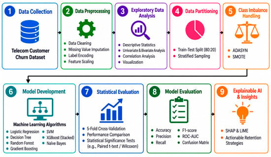
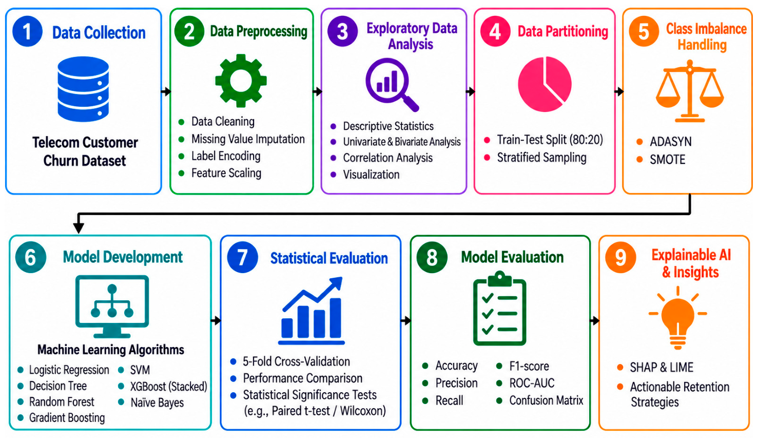
This study adopts a quantitative experimental design, which comprises nine key sequential stages, as depicted in Figure 1. As shown in Figure 1, the nine stages include data collection, preprocessing, exploratory analysis, partitioning, imbalance treatment, model development, statistical evaluation, model evaluation and explainability analysis.

Figure 1. Proposed methodology approach.

3.1. Dataset

The study uses the open-source Maven Analytics Telecom Customer Churn dataset [34] available on IBM Cognos Analytics. The dataset contains information relating to telecom subscriptions for 7043 customers. It includes 38 features covering geographical and demographic attributes, account characteristics, and service usage measures such as monthly charges, total revenue, tenure, referrals and average monthly data consumption. The records specifically identify whether customers churned, remained, or joined the service. Recent churn prediction studies have widely used and validated this dataset [32,33,35]. Table 2 summarises the attributes.

Table 2. Dataset attributes and description.

No	Attribute	Type	Description
1	Customer ID	Object	Unique customer identifier
2	Gender	Object	Customer gender
3	Age	Integer	Age in years
4	Married	Object	Marital status
5	Number of Dependents	Integer	Number of dependents
6	City	Object	City of customer’s residence
7	Zip Code	Integer	Postal customer’s code
8	Latitude	Float	Latitude of the customer’s residence
9	Longitude	Float	Longitude of customer’s residence
10	Number of Referrals	Integer	Number of customers referred
11	Tenure in Months	Integer	Months retained
12	Offer	Object	Different promotional activities offered
13	Phone Service	Object	Phone service subscription
14	Avg Monthly Long-Distance Charges	Float	Mean monthly long-distance charges
15	Multiple Lines	Object	Multiple line indicator
16	Internet Service	Object	Internet service subscription
17	Internet Type	Object	Connection type
18	Avg Monthly GB Download	Float	Mean monthly data consumption
19	Online Security	Object	Online security subscription
20	Online Backup	Object	Online backup subscription
21	Device Protection Plan	Object	Device protection indicator
22	Premium Tech Support	Object	Premium support subscription
23	Streaming TV	Object	Television streaming usage
24	Streaming Movies	Object	Film streaming usage
25	Streaming Music	Object	Music streaming usage
26	Unlimited Data	Object	Unlimited data plan indicator
27	Contract	Object	Contract type
28	Paperless Billing	Object	Electronic billing indicator
29	Payment Method	Object	Payment mechanism
30	Monthly Charge	Float	Monthly service charge
31	Total Charges	Float	Cumulative charges
32	Total Refunds	Float	Cumulative refunds
33	Total Extra Data Charges	Integer	Charges for excess data
34	Total Long-Distance Charges	Float	Cumulative long-distance charges
35	Total Revenue	Float	Cumulative revenue
36	Customer Status	Object	Stayed, churned or joined
37	Churn Category	Object	Category explaining churn
38	Churn Reason	Object	Specific reason for churn

3.2. Data Preprocessing

3.2.1. Leakage Control and Pipeline Construction

The analysis implements all preprocessing steps within a single Scikit-learn pipeline fitted only on the training fold. The pipeline estimates imputation statistics, encoder categories, and scaling parameters from the training data. This was then applied to validation and test partitions without refitting. This design prevents information leakage by ensuring that no evaluation data influences preprocessing decisions.

The target variable codes churned customers as 1 and stayers or joiners as 0. Before modelling, the pipeline removes irrelevant features, including ‘Customer ID’, ‘Churn Category’, ‘Churn Reason’, ‘City’, ‘Zip Code’, ‘Latitude’, and ‘Longitude’, because they appear only for churned customers and therefore constitute direct target leakage. The dataset comprises 7043 customer records and 38 columns, where ‘Customer Status’ is the target variable and is recoded so that both stayed and joined count as non-churners. After these exclusions, which include (1) target variables and (7) irrelevant features, the modelling dataset contains 30 predictors, which include 12 numeric variables and 18 categorical variables.

The dataset was binarised into churn and retain classes. The churned class accounts for 26.5 percent of observations against 73.5 percent for the retained class. This gives an imbalance ratio of approximately 1:2.77. This asymmetry can lead to bias towards the majority class, hence the need for imbalance treatment described in Section 3.2.5.

3.2.2. Missing-Value Treatment

A systematic missing-value audit identified structurally missing observations across several service-related attributes. The ‘offer’ variable had the highest proportion of missing values (55.05%), reflecting customers for whom no promotional offer applied. A further 21.67% of observations were missing across internet service attributes, including Avg Monthly GB Download, Internet Type, Online Security, Streaming TV, Streaming Movies, Device Protection Plan, Premium Tech Support, Streaming Music and Unlimited Data. These missing values correspond to customers without internet service and were therefore treated as structurally inapplicable rather than conventional missing observations. Similarly, Avg Monthly Long Distance and Multiple Lines had 9.68% missing values, corresponding to customers without phone service. For categorical variables, the pipeline encodes structurally inapplicable values as an explicit “not applicable” category in addition to the mode. For numeric variables, it imputes the median and adds an indicator flag to distinguish structural absence from ordinary missingness. All missing-value treatment was performed within the modelling pipeline to prevent information leakage across training and validation partitions.

3.2.3. Feature Encoding and Scaling

The categorical predictors are nominal rather than ordinal; therefore, the pipeline applies one-hot encoding rather than label encoding. This choice avoids imposing artificial distances or rank orderings that can distort linear, distance-based, and probabilistic models, including LR, SVM, K-NN, and Gaussian NB. Each categorical level is represented by a binary indicator, and unseen validation categories are handled by assigning zeros across the corresponding encoded indicators.

For numeric predictors, the pipeline standardises features to zero mean and unit variance using statistics estimated from the training fold. Standardisation makes feature magnitudes comparable for scale-sensitive algorithms. Because tree-based models are invariant to monotonic rescaling, the pipeline applies scaling only in branches connected to scale-sensitive learners and leaves boosting-model inputs unscaled.

3.2.4. Data Partitioning and Validation Design

Model comparison is performed using repeated stratified fivefold cross-validation at five epochs, giving twenty-five train and validation pairs. Repetition uses distinct random seeds so that the reported dispersion reflects partition variability rather than a single arbitrary division of the data. Hyperparameter selection is performed by inner threefold stratified cross-validation nested within each outer training fold. This is done to prevent the selection procedure from observing the data on which the resulting model is scored. In addition, a single stratified holdout of twenty percent, drawn with a fixed seed and never used for model selection, is retained as a final confirmatory test set. It is scored once, after all modelling decisions have been fixed, and it supplies the instances used for the explainability analysis reported in Section 4.6 and Section 4.7.

3.2.5. Class Imbalance Treatment

Class imbalance was addressed comparably using four treatment conditions: no resampling as the untreated baseline, class weighting, standard SMOTE, and the proposed ADASYN. Each treatment was applied only within the training portion of every outer fold. This four-arm design directly evaluates whether the observed performance of ADASYN is attributable to adaptive over-sampling or if it can be reproduced by other imbalance strategies. The final confirmatory holdout and explainability analyses used the prespecified ADASYN configuration. The number of synthetic samples G is generated according to [10] in Equations (1)–(5).

$$G=\left(n_M-n_m\right)\times \beta$$

(1)

where $n_M$ is the number of majority class instances, $n_m$ is the number of minority class instances, and $\beta \in \left[0,1\right]$ is a parameter used to specify the desired balance level after generation of the synthetic data. $\beta =1$ corresponds to full balance after the generation process.

The learning difficulty of each minority instance $x_i$ is estimated from its neighbourhood as shown in Equation (2).

$$r_i={\displaystyle \frac{{\mathsf{\Delta }}_i}{k}} i=1,\dots n_m$$

(2)

where ${\mathsf{\Delta }}_i$ is the number of majority class instances among the k-nearest neighbours of $x_i$.

The difficulty scores are normalised to a probability distribution using the standard summation form in Equation (3), where ${\hat{r}}_i$ is a density distribution $\left({\displaystyle \sum _i{\hat{r}}_i=1}\right)$

$${\hat{r}}_i={\displaystyle \frac{r_i}{{\displaystyle \sum _{i=1}^{n_m}{r}_i}}}$$

(3)

The number of synthetic samples to be generated for each minority instance follows in Equation (4).

$$g_i={\hat{r}}_i\times G$$

(4)

Each synthetic sample is then produced by interpolation between the minority instance $x_i$ and a randomly selected minority neighbour $x_{zi}$. The interpolation coefficient $\lambda$ is sampled from the continuous uniform distribution $U\left(0,1\right)$ as shown in Equation (5).

$$x_{new}=x_i+\left(x_{z_i-}{x}_i\right)\times \lambda$$

(5)

where $x_{new}$ is the generated synthetic sample, $x_i$ is the selected minority class instance, $x_{z_i}$ is a randomly selected minority class neighbour, and $\lambda$ is a random interpolation coefficient sample from $\in \left[0,1\right]$. The difference $\left(x_{z_i}-x_i\right)$ vector defines the direction of interpolation in the n dimensional feature space.

3.3. Classification Models

The nine classifiers that were developed and compared under an identical protocol are discussed briefly as follows:

3.3.1. Single ML Models

LR: A linear model that estimates the probability of the positive class by passing a linear combination of features through the logistic function, given in Equation (6), with parameters estimated by maximum likelihood [36].

$$P\left(y=1|x\right)={\displaystyle \frac{1}{1+e^{-\left(W^{T}x+b\right)}}}$$

(6)

where $P(y=1|x)$ is the conditional probability that the output target variable y equals 1, i.e., the positive class, given the input feature vector x. $W^{T}x+b$ is the linear combination of input features, x is the vector of input features, $W^T$ is the transpose of the weight vector, i.e., coefficients assigned to each feature, and b is the bias term.

DT: A recursive partitioning method that splits the feature space on the most discriminative attribute at each node [37]. Node impurity is measured by the Gini index in Equation (7), where K is the total number of classes in the dataset and $p_k$ is the proportion of an item belonging to class k at node t.

$$G(t)=1-{\displaystyle \sum _{k=1}^K{p}_{k,t}^2}$$

(7)

Gaussian Naïve Bayes: A probabilistic classifier that applies Bayes theorem under the assumption of conditional independence between features given the class label [38]. The assumption rarely holds exactly, but it permits low-variance parameter estimation and provides a useful probabilistic reference point.

K-NN: A non-parametric method that assigns each instance the majority label among its k-nearest neighbours in feature space [39]. Because the method depends on distance computation, uniform feature scaling is required.

SVM: A margin-based classifier that identifies the separating hyperplane maximising the margin between classes [40]. A radial basis function (RBF) kernel was used, with probability estimates obtained through Platt scaling. The SVM decision function is expressed in Equation (8).

$$f(x)={\omega }^T\varphi (x)+b$$

(8)

where $f(x)$ is the SVM decision function, $x$ is the input feature vector, and $\omega$ is the weight vector in the transformed feature space. $\varphi (x)$ is the feature mapping induced by the kernel function, and b is the intercept. The $f\left(x\right)$ determines the predicted class, while its magnitude indicates the distance from the separating hyperplane. Platt scaling was used to convert the decision scores into class probabilities.

RF: A bagging ensemble that constructs multiple decision trees on bootstrap samples with randomised feature subsets and aggregates their predictions by majority vote, as in Equation (9) [41]. Where y is the final predicted class for input x, $h_t(x)$ is the prediction of an individual decision tree t, T is the total number of trees in the ensemble, and mode () is the majority vote operator such as bagging, majority vote, and so on.

$$y=\mathit{mode}\left\{h_1\left(x\right),h_2\left(x\right),\dots ,h_T\left(x\right)\right\}$$

(9)

3.3.2. Ensemble Models

GBM: A sequential ensemble learning method that combines multiple weak learners, typically DT, to form a strong predictive model [42]. Each new learner is fitted to reduce the errors of the current ensemble by following the negative gradient of the specified loss function. The learners are then added sequentially to the existing model, with the learning rate controlling the contribution of each new learner. The stage-wise approach is expressed as in Equation (10)

$$F_m(x)=F_{m-1}\left(x\right)+\eta h_m\left(x\right)$$

(10)

where $F_m\left(x\right)$ is the prediction of the GBM after the m-th iteration, $F_{m-1}\left(x\right)$ is the prediction from the previous iteration, $h_m$ is the weak learner added at stage m and $\eta$ is the learning rate that controls the contribution of the newly added learner. Through this iterative process, GBM progressively minimises the loss function and improves the predictive performance of the ensemble.

XGBoost: An extension of gradient boosting with a regularised objective that penalises model complexity. It is given in Equation (11), while the regularisation term is shown in Equation (12) [18].

$$L^{(t)}={\displaystyle \sum _{i=1}^{n}l\left(y_i,{\hat{y}}_i^{(t-1)}+f_t(x_i)\right)}+\mathsf{\Omega } (f_t)$$

(11)

where $L^{(t)}$ is the total regularised objective function at iteration t, l is the differentiable training loss function that measures the error between the actual target and model prediction, $y_i$ is the true label for the i-th data instance, and ${\hat{y}}_i^{(t-1)}$ is the aggregated prediction for the i-th instance after the previous (t − 1) boosting rounds. $f_t(x_i)$ is the structure and output of the new tree being added at the current round t, and $\mathsf{\Omega }\left(f_t\right)$ is the regularisation term controlling model complexity.

$$\mathsf{\Omega } (f_t)=\gamma T+{\displaystyle \frac{1}{2}}\lambda {\displaystyle \sum _{j=1}^T{\omega }_j^2}$$

(12)

where $\mathsf{\Omega }\left(f_t\right)$ is the regularisation term for the newly added tree, T is the total number of leaves in the newly added tree, ${\omega }_j$ represents the output score for leaf j, $\gamma$ is the complexity penalty associated with adding leaves and represents the minimum loss reduction required for a split, and $\lambda$ is the regularisation parameter applied to the leaf weights to prevent them from growing too large. These parameters control the balance between fit to the training data and model complexity.

LightGBM: A gradient boosting framework employing histogram-based split finding, gradient-based one-side sampling and leaf-wise tree growth, which reduce training time and memory consumption while preserving accuracy [19]. Its prediction is the weighted sum of tree outputs in Equation (13).

$$F_M(x)={\displaystyle \sum _{m=1}^M\nu f_m(x)}$$

(13)

where $F_M(x)$ is the final ensemble prediction for input x after all M trees have been evaluated and combined, M is the total number of trees constructed in the ensemble, $\nu$ is the shrinkage weight (or learning rate), which scales down the contribution of each individual tree to prevent overfitting, and $f_m(x)$ is the prediction output of the individual weak learner (leaf-wise tree) trained at stage m.

3.4. Model’s Parameter Configuration

As shown in Table 3, hyperparameters are selected by randomised search within each outer training fold using inner threefold stratified cross-validation and F1 as the selection criterion. F1 is used because the churn class represents only 26.5% of observations and the study prioritises balanced identification of churners rather than accuracy dominated by the majority class. The search ranges were chosen to cover low, moderate and higher model complexity while keeping the search computationally tractable. For LR and SVM, C controls regularisation strength; for DT and RF, depth and split controls regulate tree complexity; for K-NN, neighbourhood size and distance weighting control local smoothness; for GBM, XGBoost and LightGBM, the search jointly varies the number of boosting stages, learning rate and tree complexity. The final configuration is therefore selected from data-driven validation rather than manual selection or optimisation against the test set. The modal configuration across the 25 outer folds is reported in Table 3.

Table 3. Model categories and selected hyperparameters.

Model	Hyperparameter Search Space	Model Selected Configuration
LR	C ∈ {0.01, 0.1, 1, 10, 100}	{“C”: 10}
DT	min_samples_split ∈ {2, 5, 10}; max_depth ∈ {3, 4, 5, 8, 10, None}	{“min_samples_split”: 2, “max_depth”: 4}
Gaussian NB	var_smoothing ∈ {1 × 10−9, 1 × 10−8, 1 × 10−7, 1 × 10−6}	{“var_smoothing”: 1 × 10−9}
K-NN	weights ∈ {uniform, distance}; n_neighbors ∈ {3, 5, 7, 9, 11, 15}	{“weights”: “distance”, “n_neighbors”: 11}
SVM	gamma ∈ {0.001, 0.01, 0.1, scale}; C ∈ {0.1, 1, 10}	{“gamma”: 0.01, “C”: 10}
RF	n_estimators ∈ {100, 200, 500}; max_features ∈ {sqrt, log2}; max_depth ∈ {5, 10, 20, None}	{“n_estimators”: 200, “max_features”: “sqrt”, “max_depth”: 10}
GBM	n_estimators ∈ {100, 200, 300}; max_depth ∈ {3, 4, 5}; learning_rate ∈ {0.01, 0.05, 0.1}	{“n_estimators”: 100, “max_depth”: 4, “learning_rate”: 0.05}
XGBoost	subsample ∈ {0.8, 1.0}; n_estimators ∈ {100, 200, 300}; max_depth ∈ {3, 6, 9}; learning_rate ∈ {0.01, 0.05, 0.1}	{“subsample”: 1.0, “n_estimators”: 100, “max_depth”: 6, “learning_rate”: 0.05}
LightGBM	num_leaves ∈ {15, 31, 63}; n_estimators ∈ {100, 200, 300}; learning_rate ∈ {0.01, 0.05, 0.1};	{“num_leaves”: 15, “n_estimators”: 100, “learning_rate”: 0.05}

All twenty-five outer folds used identical partitions across classifiers, ensuring paired comparisons. Differences between the selected model and each competing classifier were evaluated using the Wilcoxon signed-rank test on fold-level F1-scores. Multiple comparisons were controlled using the Holm correction. Effect size was quantified using Cohen’s ($d_z$), calculated as the mean of the paired fold-level differences divided by the standard deviation of those differences. Effect sizes were reported alongside the statistical tests because, with twenty-five paired observations, statistical significance may not necessarily indicate practically meaningful performance differences. Given that repeated cross-validation observations are not fully independent, the Wilcoxon results were interpreted as supplementary paired evidence rather than definitive confirmatory inference, consistent with concerns regarding resampling-based statistical testing [43].

3.5. Evaluation Metrics

The model performance is assessed using the following key metrics: accuracy, precision, recall, F1-score and ROC-AUC. Accuracy measures the percentage of correct classifications to the total classifications made. Precision estimates the probability that a positive prediction is correct. High precision means a low false-positive rate. Recall measures the positive instances that are correctly classified. F1-score combines precision and recall. It can be defined as the average value of precision and recall. ROC-AUC measures discriminative ability across all classification thresholds. PR-AUC summarises the trade-off between precision and recall across all classification thresholds. Mathematically, the six metrics can be expressed in Equations (14)–(19), respectively.

$$Accuracy={\displaystyle \frac{TP+TN}{TP+TN+FP+FN}}$$

(14)

$$\mathrm{Pr}ecision={\displaystyle \frac{TP}{TP+FP}}$$

(15)

$$\mathrm{Re}call={\displaystyle \frac{TP}{TP+FN}}$$

(16)

$$F1-Score=2\times \left({\displaystyle \frac{\mathrm{Pr}ecision\times \mathrm{Re}call}{\mathrm{Pr}ecision+\mathrm{Re}call}}\right)$$

(17)

$$ROC-AUC={\displaystyle {\int }_0^{1}TPR(FPR)d(FPR)}$$

(18)

$$PR-AUC={\displaystyle {\int }_0^{1}P(R)dR}$$

(19)

where TP refers to true positives, TN is true negatives, FP is false positives and FN is false negatives.

PR-AUC is reported because, under class imbalance, ROC-AUC is insensitive to changes in the false positive count relative to a large majority class, and it can present an optimistic picture of minority class performance. The baseline PR-AUC for a random classifier equals the positive class prevalence, which is 0.265 for this dataset; the reported PR-AUC values should be interpreted relative to this baseline. Threshold-dependent metrics were calculated using an F1-optimised threshold selected on the training folds rather than the default 0.5, which may be inappropriate after resampling. Brier Score evaluates the accuracy of predicted churn probabilities, with lower values indicating better probability calibration. The classification threshold determines the probability cutoff used to classify customers as churners and influences the trade-off between precision and recall.

3.6. Explainability Design

The interpretability layer is applied to the best-performing model, based on the deployed performance metrics. The interpretability layer is designed to serve two organisational decision levels, namely:

• At the strategic level, SHAP TreeExplainer is applied to the fitted model to obtain global feature attribution. Four complementary views are generated, namely (a) a beeswarm summary showing the distribution and direction of feature effects, (b) a bar plot ranking features by mean absolute Shapley value, (c) a waterfall plot decomposing an individual prediction relative to the model base value, and (d) dependence plots showing the interaction structure for the two highest-ranked features.
• At the operational level, LIME is configured as a tabular explainer in classification mode. The model is fitted on the unresampled training distribution. This approach ensures that the resulting explanations reflect the characteristics of real customers rather than those of a synthetically augmented population. Instance-level explanations are generated for a correctly classified churner and for a misclassified churner. The latter is chosen because FN correspond to the customers that a retention programme would fail to reach.

The rationale for retaining both techniques is that they are complementary in form as well as in scope. SHAP provides attribution with a defined axiomatic basis, while LIME produces coefficient-like output that resembles the regression summaries familiar to CRM analysts. The division is architectural rather than decorative: global attribution informs policy design, and local attribution informs case-level communication.

Explanations were treated as empirical outputs and not assumed reliable to make the explainability framework trustworthy. Three complementary properties were evaluated: local fidelity, stability and cross-technique agreement. Local fidelity was quantified by comparing LIME surrogate predictions to model predictions on 200 test instances sampled locally via the coefficient of determination (R²). To assess stability, each LIME explanation was regenerated 10 times with different random seeds, and the consistency of the rankings of features from each LIME explanation was quantified by calculating the Jaccard similarity and rank correlation. The Spearman rank correlation was calculated between SHAP and LIME feature attribution vectors at each instance.

3.7. Computational Environment and Reproducibility

All experiments were conducted in Python 3.13.5 using Scikit-learn, imbalanced-learn, XGBoost, LightGBM, SHAP and LIME, with NumPy 2.1.3 and pandas 2.2.3 for data handling and Matplotlib 3.10.0 and Seaborn 0.13.2 for visualisation. The complete pipeline, including preprocessing, resampling, tuning, evaluation, statistical testing and figure generation, is executed by a single script. Algorithm 1 summarises the experimental procedure.

Algorithm 1. Experimental procedure
Step	Operation
1	Load dataset; binarise target as churned = 1, stayed or joined = 0
2	Drop identifier and leakage bearing columns
3	For each of 5 repetitions and each of 5 stratified outer folds:
4	Fit preprocessing pipeline on the training fold: impute, one-hot encode, scale
5	Apply the assigned imbalance treatment to the training fold only; assert disjointness from the validation fold
6	Select hyperparameters by inner threefold cross-validation optimising F1
7	Train each model on the resampled training fold
8	Select the decision threshold on the training fold by maximising F1
9	Score the validation fold; record accuracy, precision, recall, F1, ROC-AUC, PR-AUC and the Brier score
10	Aggregate across folds; report mean and standard deviation; apply Wilcoxon signed-rank tests with Holm correction
11	Refit the selected model on the full development set; score the confirmatory holdout once
12	Apply SHAP and LIME to the refitted model; compute fidelity, stability and agreement
13	Write all tables and figures to file

4. Results and Discussion

4.1. Exploratory Data Analysis

4.1.1. Customer Status and Churn Distribution

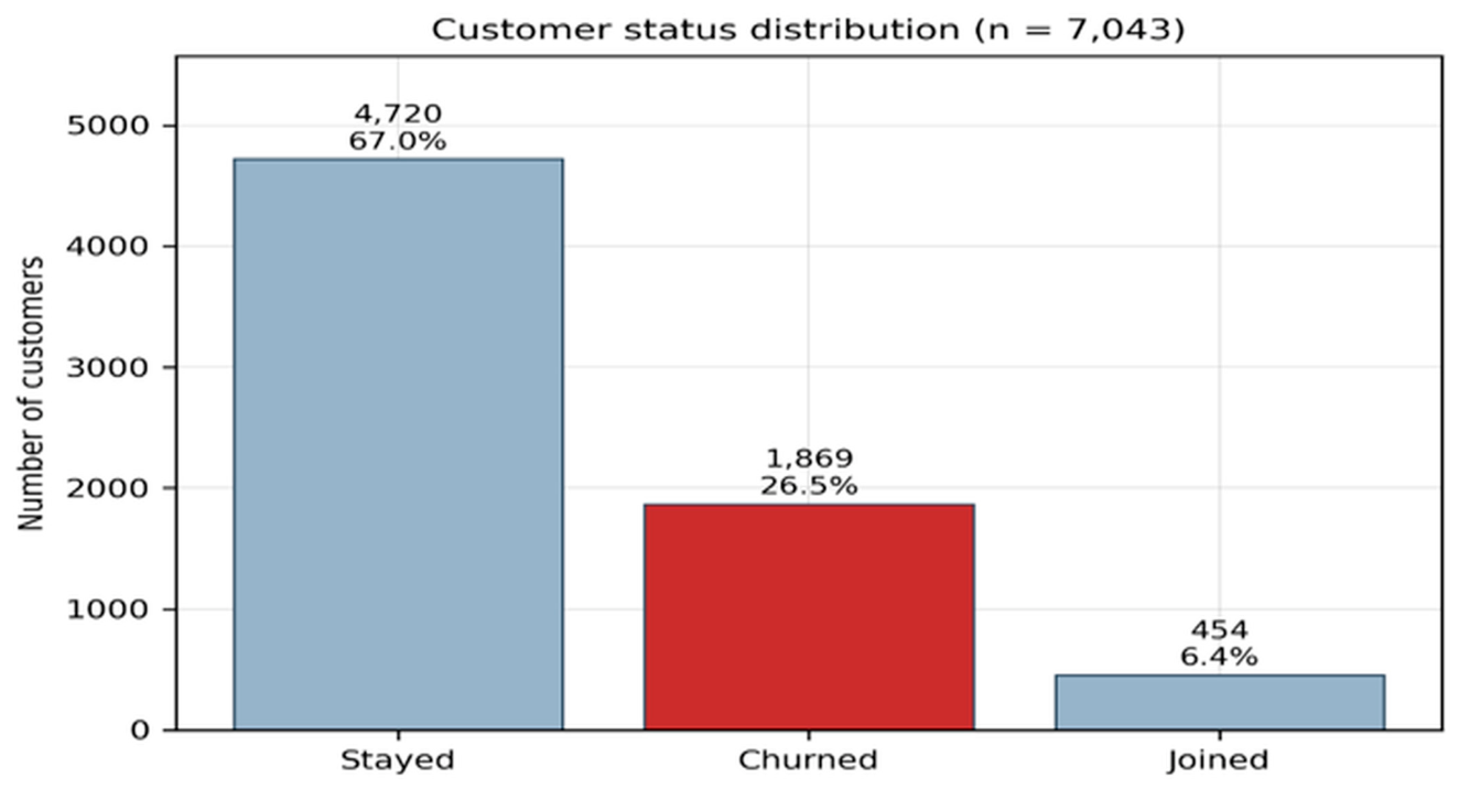
Figure 2 presents the original dataset’s distribution of customer churn status. The original dataset comprises 7043 customers, of whom 67.0% (n = 4720) remained with the provider, 26.5% (n = 1869) churned and 6.4% (n = 454) had newly joined. Initial preprocessing towards binary labelling yields 73.5% (n = 5174) non-churn and 26.5% churn (n = 1869). This asymmetric data structure motivates the imbalance treatment described in Section 3.2.5.

Figure 2. Original dataset distribution of customer churn status.

4.1.2. Churn Patterns Across Categorical Attributes

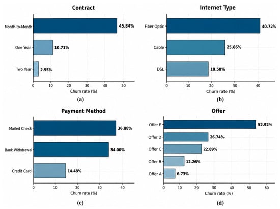
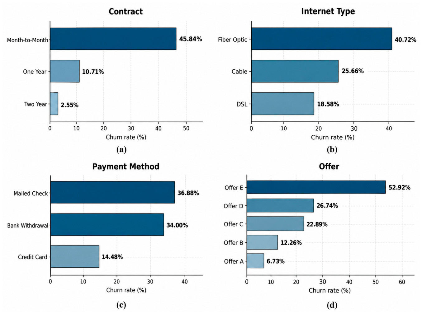
Figure 3 reports churn rates across categorical attributes. Contract type provides the clearest categorical separation: “month-to-month” customers churn at a markedly higher rate than “one-year” customers (10.71%) and “two-year” customers (2.95%). This gradient indicates that contractual commitment increases switching costs and reduces attrition risk. Other categorical variables reveal complementary risk patterns. “Fibre optic” subscribers record the highest churn rate (40.72%), followed by “cable” (25.66%) and “DSL” (18.58%). This suggests that service technology differentiates perceived value or service experience. Payment method shows a similar gradient: “mailed cheque” (36.86%) and “bank withdrawal” (34.00%) substantially exceed “credit card” (14.48%). This indicates that automated digital payment may operate as a retention-supportive behaviour. Promotional offers also differ sharply, ranging from 52.92% churn under “Offer E” to 6.73% under “Offer A”, which suggests that retention incentives may vary materially in quality or customer targeting.

Figure 3. Churn rate by categorical attribute.

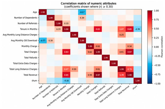
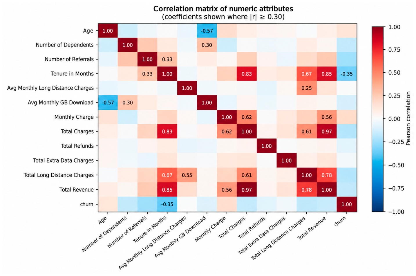
The correlation structure in Figure 4 confirms strong collinearity between “Total Charges” and “Total Revenue” (r > 0.85) and between “Monthly Charge” and “Total Charges” (r > 0.70). While this does not impair tree-based gradient boosting (which handles correlated inputs internally), it does explain the proximity of these attributes in the attribution rankings reported in Section 4.6, since they encode a single underlying economic dimension rather than independent signals.

Figure 4. Feature correlation matrix.

4.2. Effect of ADASYN on the Imbalance Dataset

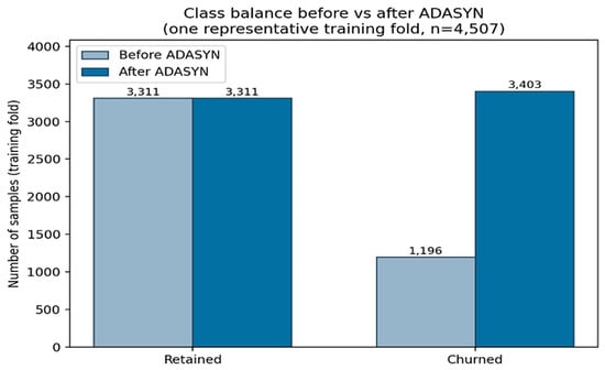
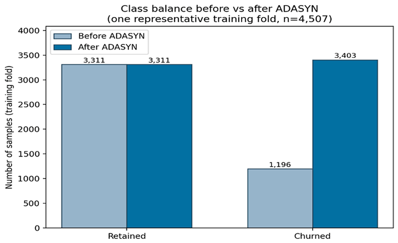
Figure 5 provides a validated accounting of the ADASYN resampling results on the training set. Within a representative inner training fold (n = 4507), the pre-resampling class distribution comprised 3311 non-churned and 1196 churned instances (an imbalance ratio of 2.769:1). Achieving exact parity as defined in Equation (1), with β = 1, would require 2115 additional synthetic minority samples. Consistent with the density-adaptive weighting described in Equations (2)–(4), ADASYN generated 2207 synthetic samples (92 more than the exact-parity target). This brings the post-resampling training distribution to 3403 churned versus 3311 non-churned instances (ratio ≈ 1:1.028). This overshoot reflects the neighbourhood-weighted generation mechanism described in Section 3.2.5.

Figure 5. Class distribution after addressing class imbalance issue using ADASYN.

4.3. Comparative Analysis of Imbalance Treatment Methods

Table 4 reports the F1-score and PR-AUC of the nine classifiers under the four imbalance treatment methods. The results are averaged across the twenty-five outer folds with no resampling serving as the baseline. The effect of imbalance treatment varied across the nine classifiers. ADASYN achieved the highest F1-score for LightGBM (0.7212) and XGBoost (0.7316). For LightGBM, ADASYN also produced the highest PR-AUC (0.7916), with SMOTE (0.7912) being second best. These results demonstrate that the effect of imbalance treatment is classifier-dependent. Also, these results showed that improvement in F1-score does not necessarily occur uniformly across evaluation metrics. Lastly, findings indicate that the effectiveness of imbalance treatment is model-dependent rather than universally improved by adaptive over-sampling. Class weighting was evaluated only where the corresponding weighting mechanism was explicitly configured. LightGBM supports a class weight parameter because it was not independently configured in the reported analysis. Consequently, its class-weighting results are identical to the no resampling baseline and are not interpreted as an independent class-weighting experiment. For models without this capability, the class-weighting and no resampling conditions are therefore identical.

Table 4. Mean F1-score and PR-AUC of nine classifiers under four imbalance-treatment conditions across 25 outer folds.

Model	F1 None	F1 Class Weights	F1 SMOTE	F1 ADASYN	PR-AUC None	PR-AUC Class weights	PR-AUC SMOTE	PR-AUC ADASYN
DT	0.6521	0.6774	0.6563	0.6515	0.6480	0.6689	0.6182	0.6069
Gaussian NB	0.6716	0.6716	0.6748	0.6691	0.6825	0.6825	0.6872	0.6800
GBM	0.7146	0.7146	0.7097	0.7105	0.7892	0.7892	0.7859	0.7863
K-NN	0.5867	0.5867	0.5703	0.5346	0.6604	0.6604	0.6148	0.5708
LightGBM	0.7159	0.7159	0.7189	0.7212	0.7884	0.7884	0.7912	0.7916
LR	0.7060	0.7027	0.7042	0.7035	0.7598	0.7573	0.7564	0.7509
RF	0.7013	0.7020	0.6955	0.6944	0.7696	0.7628	0.7423	0.7461
SVM	0.7049	0.6824	0.6957	0.6850	0.7661	0.7459	0.7416	0.7246
XGBoost	0.7110	0.7110	0.7111	0.7136	0.7888	0.7888	0.7869	0.7855

4.4. Model Performance Comparison

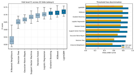
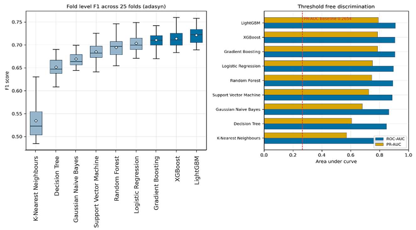
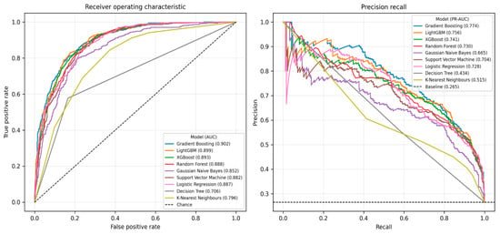
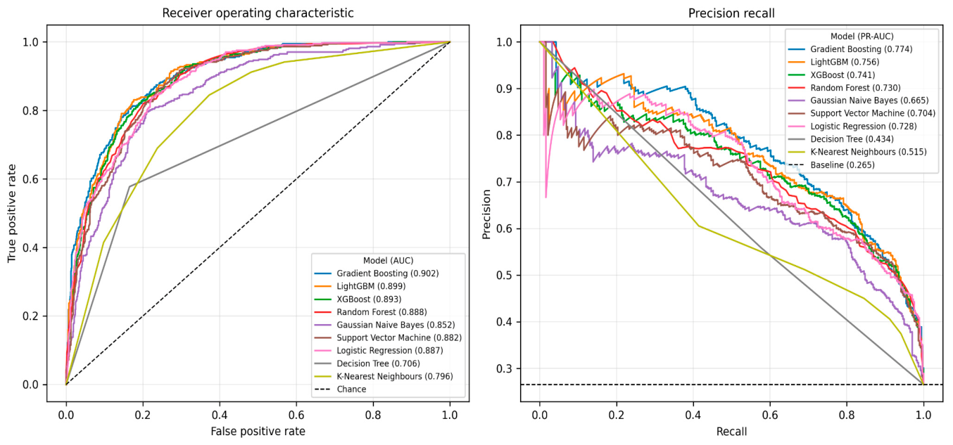
Table 5 reports the full evaluation for all nine classifiers after using ADASYN to address the class imbalance. This was aggregated across the twenty-five outer folds. Figure 6 presents the repeated-cross-validation fold-level performance, whereas Figure 7 shows the receiver operating characteristic and precision-recall curves computed on the independent 20% confirmatory holdout set. Therefore, the ROC-AUC and PR-AUC values shown in Figure 7 are not expected to equal the cross-validated means reported in Table 5 because they are based on different evaluation sets. This also presents a slight difference in the ranking of LightGBM and GBM: LightGBM achieved a higher mean ROC-AUC than GBM in the repeated cross-validation results (0.9094 versus 0.9068), whereas GBM achieved a slightly higher ROC-AUC than LightGBM on the independent holdout set (0.902 versus 0.899). This difference shows variation between the cross-validation estimates and the independent holdout evaluation rather than an inconsistency in the reported results. The repeated cross-validation results in Table 5 were used as the primary basis for comparative model evaluation, while Figure 7 provides an independent confirmatory assessment. As shown in Table 5, LightGBM achieved the highest mean F1-score (0.7212) and the highest mean ROC-AUC (0.9094) and PR-AUC (0.7916) and the lowest Brier score (0.1054). This superior performance can be attributed to its efficient gradient boosting architecture, leaf-wise tree growth, and ability to capture complex feature interactions and nonlinear relationships [19]. The three boosting ensembles consistently ranked among the strongest classifiers across the evaluation metrics, with relatively small differences in their F1-scores. The other models also demonstrated competitive performance, with LR trailing the best-performing ensemble by only 0.018 F1 points. On the other hand, K-NN had a high fold-to-fold variability and a poor ranking, as seen by its low PR-AUC (0.5708). The PR-AUC achieved by LightGBM was approximately three times the random-classifier baseline of 0.2654, demonstrating strong ability to rank customers according to their estimated churn risk.

Table 5. Performance of nine classifiers under ADASYN, reported as mean values with standard deviations across 25 folds.

Model	Accuracy	Precision	Recall	F1	ROC-AUC	PR-AUC	Brier	Threshold
LR	0.8325 (0.0123)	0.6642 (0.0252)	0.7489 (0.0307)	0.7035 (0.0198)	0.8958 (0.0108)	0.7509 (0.0316)	0.1436 (0.0067)	0.6890 (0.021)
DT	0.7892 (0.0130)	0.5815 (0.0225)	0.7429 (0.0411)	0.6515 (0.0190)	0.8477 (0.0129)	0.6069 (0.0278)	0.1472 (0.0075)	0.3940 (0.050)
Gaussian NB	0.7927 (0.0135)	0.5812 (0.0218)	0.7893 (0.0248)	0.6691 (0.0169)	0.8644 (0.0117)	0.6800 (0.0251)	0.2108 (0.0133)	0.9040 (0.081)
K-NN	0.5770 (0.1236)	0.4051 (0.0972)	0.8882 (0.1654)	0.5346 (0.0421)	0.8246 (0.0212)	0.5708 (0.0407)	0.2178 (0.0090)	0.2100 (0.291)
SVM	0.8257 (0.0101)	0.6586 (0.0207)	0.7155 (0.0442)	0.6850 (0.0225)	0.8876 (0.0114)	0.7246 (0.0336)	0.1340 (0.0074)	0.6520 (0.030)
RF	0.8282 (0.0124)	0.6579 (0.0236)	0.7361 (0.0319)	0.6944 (0.0223)	0.8915 (0.0120)	0.7461 (0.0292)	0.1178 (0.0069)	0.4720 (0.024)
GBM	0.8384 (0.0131)	0.6803 (0.0372)	0.7469 (0.0392)	0.7105 (0.0167)	0.9068 (0.0102)	0.7863 (0.0233)	0.1080 (0.0062)	0.4580 (0.031)
XGBoost	0.8405 (0.0114)	0.6828 (0.0287)	0.7493 (0.0357)	0.7136 (0.0189)	0.9063 (0.0098)	0.7855 (0.0224)	0.1084 (0.0059)	0.4620 (0.041)
LightGBM	0.8430 (0.0109)	0.6827 (0.0245)	0.7659 (0.0375)	0.7212 (0.0193)	0.9094 (0.0101)	0.7916 (0.0232)	0.1054 (0.0059)	0.4170 (0.026)

Figure 6. Comparison of classifier performance with fold-level dispersion.

Figure 7. Receiver operating characteristics and precision-recall curves for all classifiers on the independent 20% confirmatory holdout set; values are distinct from the repeated cross-validation estimates reported in Table 5.

4.5. Statistical Comparison of Models

Table 6 presents a structured comparison of the overall best performer (LightGBM) against each competing classifier, combining repeated nested cross-validation with paired Wilcoxon signed-rank tests and Holm correction.

Table 6. Paired comparison of LightGBM against each competing classifier with Wilcoxon signed-rank tests and Holm correction with effect sizes across 25 outer folds.

Comparison	Mean F1 Difference	Wilcoxon p (Uncorrected)	Effect Size (Cohen’s dz)	Effect Size (Rank Biserial r)	Wilcoxon p (Holm Corrected)
LightGBM vs. DT	0.0697	0	4.8426	1	0
LightGBM vs. Gaussian NB	0.0521	0	4.0795	1	0
LightGBM vs. K-NN	0.1866	0	4.7002	1	0
LightGBM vs. SVM	0.0362	0	2.2744	1	0
LightGBM vs. RF	0.0267	0	1.7892	1	0
LightGBM vs. LR	0.0177	0	1.3339	0.92	0
LightGBM vs. GBM	0.0106	0.0005	0.8928	0.7538	0.001
LightGBM vs. XGBoost	0.0075	0.0038	0.6898	0.6431	0.0038

As shown in Table 6, Wilcoxon signed-rank results detect significant paired differences between LightGBM and all competing classifiers after Holm correction. However, the 25-fold-level estimates generated through repeated cross-validation are paired but are not statistically independent because observations can recur across training and validation partitions. Accordingly, these p-values are interpreted as supplementary evidence rather than definitive confirmatory inference. This is consistent with established concerns regarding resampling-based significance testing [43]. The magnitude of the observed differences is therefore considered alongside the effect sizes. In particular, the F1-score advantages of LightGBM over XGBoost (0.0075) and Gradient Boosting (0.0106) are modest despite statistically significant paired differences. The Wilcoxon analysis therefore does not establish clear superiority of LightGBM over the leading boosting models. Rather, the results support the interpretation that the boosting classifiers form the strongest-performing group, with relatively small performance differences among the leading models.

4.6. Comparison of Previous Studies

Table 7 compares the present study with recently published studies on customer churn prediction. The present study evaluated nine classifiers (LR, DT, NB, K-NN, SVM, RF, GBM, XGBoost, LightGBM) under four imbalance methods, while the comparative metrics reported in Table 7 correspond specifically to the results from the LightGBM-ADASYN configuration. This configuration achieved an F1-score of 72.12%, an ROC-AUC of 0.9094 and a PR-AUC of 0.7916.

Table 7. Comparison with previous studies on customer churn prediction using comparable telecommunications datasets.

Study	Dataset	Model	Accuracy	Precision	Recall	F1	ROC-AUC	PR-AUC
[24]	Maven Analytics Telecom Customer Churn	RF	86.94	-	85.47	-	95.00	-
[33]	Telco Systems	RF	82.00	82.00	-	83.00	84.00	-
[9]	Telecom customer churn	XGBoost (75:25 balancing)	89.60	76.04	62.82	68.81	-	-
Present study	Maven Analytics Telecom Customer Churn -	LightGBM+ADASYN	0.8430	0.6827	0.7659	72.12	90.94	79.16

Compared with [9], the F1-score result achieved by the LightGBM model was higher than 68.81% for XGBoost. Also, [24] reported an accuracy of 86.94% and an ROC-AUC of 95.00% for RF, while [33] reported an F1-score of 83.00% and an ROC-AUC of 84.00%. However, these results are not directly comparable because the studies used different models, imbalance methods, preprocessing procedures and validation protocols. The present study therefore provides a controlled within-dataset comparison of nine classifiers across four imbalance method treatments, complemented by SHAP and LIME for model interpretability.

4.7. Global Attribution Analysis

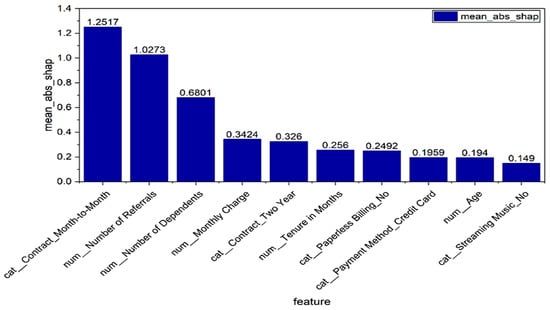
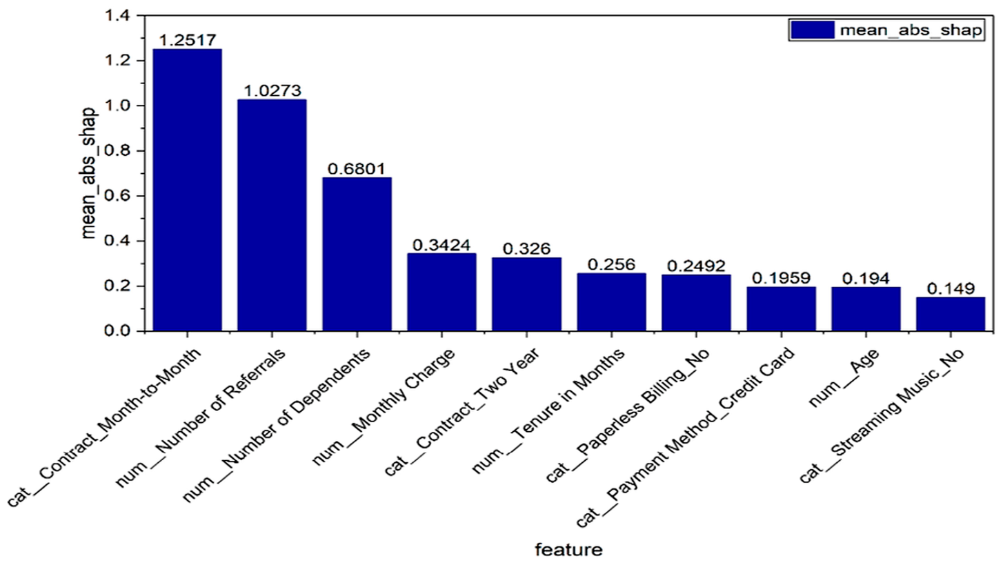
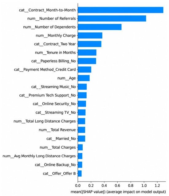
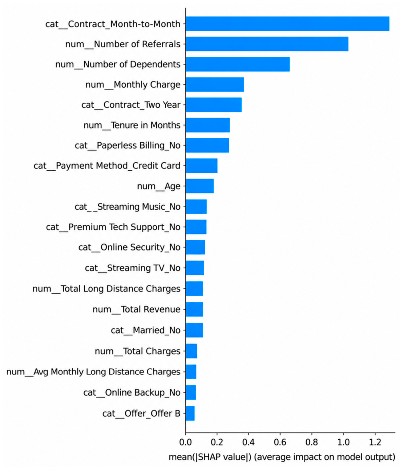
SHAP TreeExplainer was applied to the best performer (fitted LightGBM model) over a sample of holdout instances. Figure 8 reports the mean absolute Shapley value results for the ten highest-ranked features.

Figure 8. Global feature attribution result.

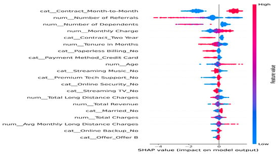
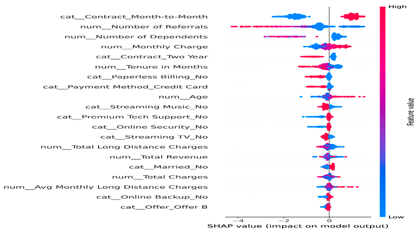
Figure 8 depicts the global feature attribution. The analysis demonstrates that the LightGBM model relies primarily on “contract type” and “referral behaviour” for predicting customer churn. Also, Figure 9 presents the SHAP beeswarm summary result for the LightGBM. As shown in Figure 9, “month-to-month contract” exhibits the highest mean absolute SHAP value, indicating that it contributes more to the model’s predictions than any other feature. Customers on “month-to-month” contracts generally have positive SHAP values, reflecting an increased likelihood of churn, whereas customers on longer-term contracts contribute negatively to the prediction, indicating a lower churn risk. The number of “referrals” is the second most influential feature, with higher referral counts consistently associated with lower churn probabilities. This finding suggests that “referral behaviour” captures customer satisfaction and engagement, making it a valuable behavioural indicator for identifying loyal customers. From a CRM perspective, encouraging customer referrals may therefore serve not only as an acquisition strategy but also as an indicator of customer retention.

Figure 9. SHAP beeswarm summary for LightGBM.

Figure 10 presents the SHAP-ranked feature importance result. As shown in Figure 10, the ranked SHAP feature importance result confirms that “contract type” and “referrals” dominate the prediction process, followed by “dependents”, “monthly charges”, “internet service”, and “tenure”. Although “tenure” is widely recognised as an important churn predictor, its relatively lower ranking indicates that its predictive contribution overlaps with “contract type”. SHAP distributes attribution among correlated variables so that part of the importance traditionally attributed to “tenure” can be attributed to “contract type” and not only to tenure.

Figure 10. SHAP ranked feature importance.

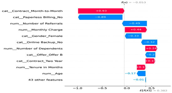
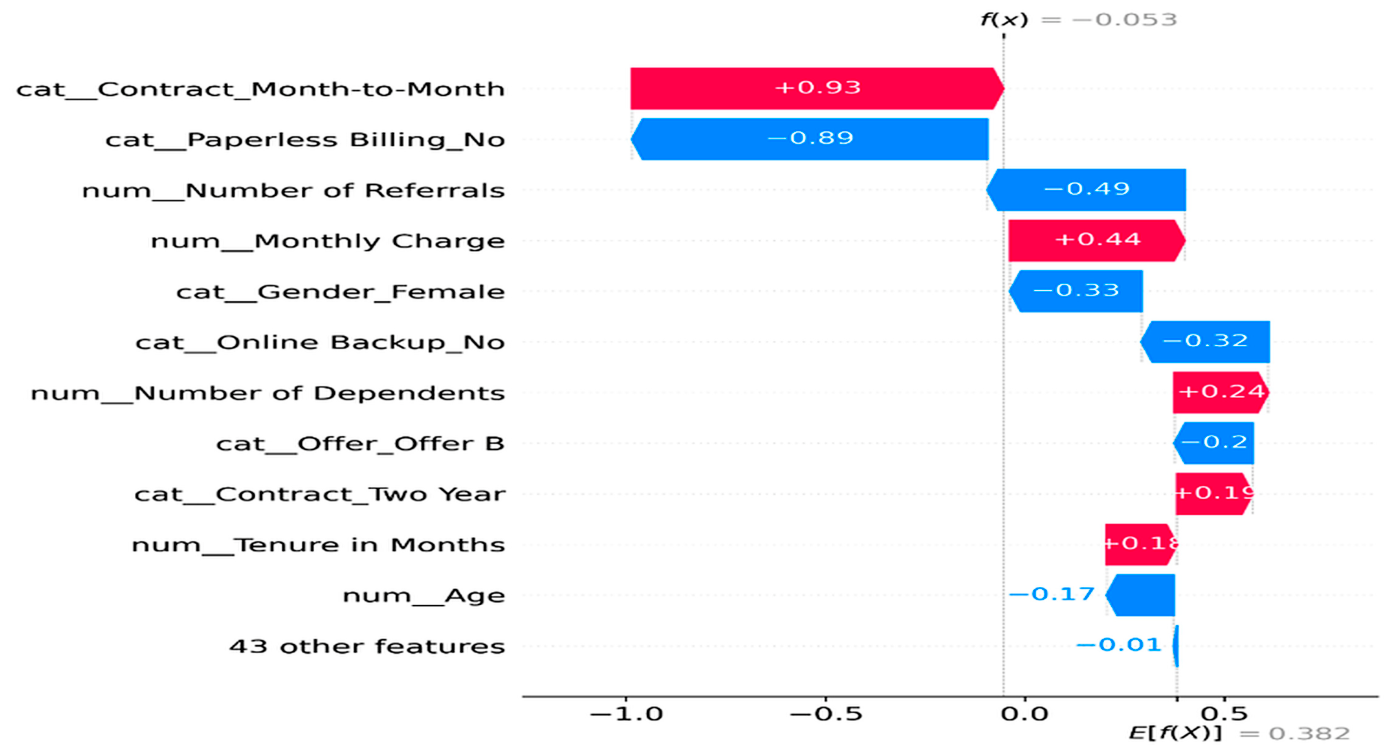
Furthermore, the SHAP waterfall plot in Figure 11 provides an instance-level explanation by decomposing an individual prediction into additive feature contributions. Features with positive SHAP values increase the predicted probability of churn, whereas negative SHAP values reduce it. The cumulative contribution of these features moves the prediction from the model’s baseline output to the final classification, thereby illustrating the rationale behind the model’s decision for a specific customer. This level of transparency enables practitioners to understand why a customer is predicted to churn and supports the design of targeted retention interventions.

Figure 11. SHAP waterfall decomposition of a correctly classified churner.

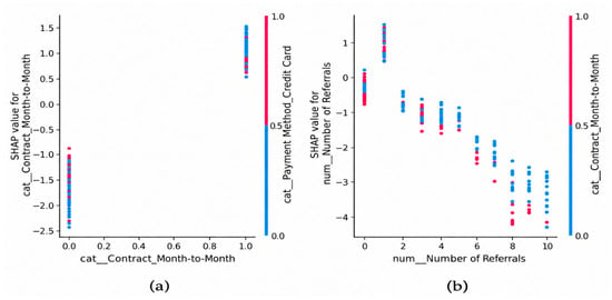
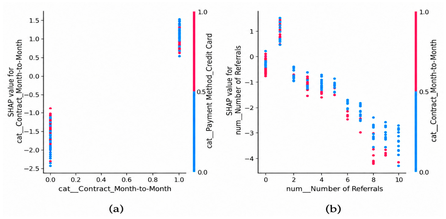
Figure 12 shows that a higher number of “referrals“ is generally associated with increasingly negative SHAP values, indicating a lower predicted churn risk, while “month-to-month” contracts produce strongly positive SHAP values and therefore contribute substantially to higher churn risk. The interaction patterns further suggest that the effects of “referrals” and “contract type” vary across customer characteristics, highlighting the importance of feature interactions in explaining churn predictions.

Figure 12. SHAP dependence plots for top two high-ranked features: (a) month-to-month contract and (b) number of referrals.

4.8. Case-Level Attribution Analysis

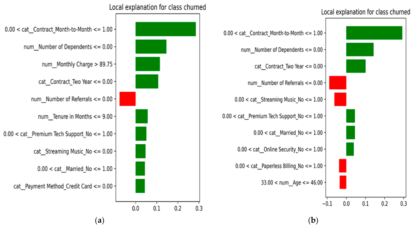
LIME was applied at the operational level to translate individual predictions into practitioner-readable reasoning. Figure 13a,b present two cases involving correctly and incorrectly classified churners. Figure 13a demonstrates the reasoning behind a successful churn prediction, whereas Figure 13b illustrates a misclassified churner drawn from the 119 false negatives, revealing the boundary at which the learned pattern fails.

Figure 13. LIME explanation for (a) correctly classified churned and (b) misclassified churner.

The local surrogate for the correctly classified churner attains a fidelity of R² = 0.4071, and the surrogate for the false-negative case attains R² = 0.3927. These values are reported alongside the explanations because they bound how much confidence the case narratives warrant. A surrogate that accounts for roughly 40% of the local variation in model output provides useful insight into the direction of the principal contributions. However, it does not fully capture the model’s behaviour at that point. The false-negative case provides greater diagnostic value than the correctly classified case. When churn-enhancing behavioural signals are offset by retention-favourable transactional signals, the model may favour the retention-related evidence and consequently misclassify the customer as a non-churner. This class of customer is precisely the group for which model scores alone are insufficient and supplementary qualitative monitoring is warranted. This specifically constitutes 32 percent of the actual churners in the holdout at the tuned threshold.

Table 8 presents the measured explanation quality for LightGBM. The results in Table 8 are computed over 200 sample holdout instances with stability assessed over ten random restarts on a subset of twenty instances.

Table 8. Measured explanation quality for LightGBM.

Property	Mean	SD
Local fidelity (surrogate R2)	0.4410	0.0546
Stability (top-5 Jaccard)	0.9567	0.1121
Stability (weight rank correlation)	0.8851	0.0689
SHAP-LIME agreement (Spearman)	0.5245	0.0624

The interpretability layer was evaluated using local fidelity, stability and cross-technique agreement as shown in Table 7. The mean top-five Jaccard similarity was 0.9567, and the mean feature-weight rank correlation was 0.8851, indicating high LIME stability. Local fidelity was moderate (R² = 0.441), while SHAP-LIME agreement was also moderate (Spearman ρ = 0.5245). These results support the use of SHAP and LIME as complementary tools. SHAP is well suited to global driver analysis, while LIME is useful for case-level communication. However, neither method should be treated as a causal explanation or as proof that other methods are correct.

4.9. From Prediction to Strategic Action

The attribution results in Figure 8 were translated into explicit, rule-based CRM heuristics rather than treated solely as descriptive rankings. ‘Month-to-month’ contract status was the strongest global driver (mean absolute Shapley value = 1.2517), followed by ‘referral activity’ (1.0273), while monthly charge (0.3424) and tenure (0.2560) also contributed to churn prediction. These variables can therefore serve as routing signals within CRM systems. However, they should not be interpreted as causal triggers. The model probability remains the primary score. SHAP and LIME provide complementary reason codes for selecting appropriate interventions. Table 9 presents the proposed operational rules and corresponding managerial actions. For the reported LightGBM configuration, the cross-validated F1 threshold was approximately 0.417. This threshold is specific to the model, study dataset and should not be interpreted as a universal business benchmark. In a production environment, the threshold should be recalibrated according to intervention costs, customer lifetime value (CLV), offer acceptance, retention uplift and available operational capacity.

Table 9. Operational CRM decision rules derived from the LightGBM.

Rule	Predictive Condition	CRM Decision Rule	Managerial Action
Rule 1	Predicted churn probability ≥ 0.417; ‘month-to-month’ contract	IF predicted churn probability ≥ 0.417 AND Contract = ‘Month-to-month’ THEN route the customer to a retention review queue.	Consider marketing strategies that target contract migration
Rule 2	Predicted churn probability ≥ 0.417; zero ‘referral activity’	IF predicted churn probability ≥ 0.417 AND Number of Referrals = 0, THEN flag the customer for engagement or service -experience review.	Review customer engagement and encourage post-service review before considering an incentive.
Rule 3	Predicted churn probability ≥ 0.417; ‘Month-to-month’ contract; zero or low ‘referral activity’	IF predicted churn probability ≥ 0.417 AND Contract = ‘Month-to-month’ AND Number of Referrals = 0 or low, THEN assign higher retention priority.	Conduct a targeted customer review, segment and prioritise an appropriate retention strategy.
Rule 4	Predicted churn probability ≥ 0.417; relatively high monthly charge	IF predicted churn probability ≥ 0.417 AND Monthly Charge is relatively high, THEN assess plan, bundle, or price sensitivity.	Review marketing strategies related to plans, bundles, and pricing before offering financial incentives.

The rules in Table 9 provide a direct pathway from model prediction to CRM action. The broader strategic implications of the identified rules are presented in Table 10. Global attribution can support resource allocation and policy design, whereas case-level explanations support targeted frontline interventions. For instance, month-to-month contracts may inform both targeted migration strategies and longer-term review of commitment structures. Similarly, referral activity can be incorporated as a behavioural monitoring signal, while elevated monthly charges can trigger value communication and bundle reviews. These findings should be interpreted as decision-support mechanisms rather than as evidence of causal effects.

Table 10. Proposed CRM retention decision framework linking measured churn drivers to tactical and structural responses.

Identified Driver	Evidential Basis	Tactical CRM Intervention	Structural Business Response
Month-to-month contract	Highest attribution; mean absolute SHAP = 1.2517	Targeted migration offers and commitment incentives	Redesign commitment pricing and reduce switching barriers
Tenure	SHAP = 0.2560; tenure-related separation	Structured onboarding and milestone retention contacts	Establish the first year as a dedicated customer lifecycle stage
Elevated monthly charge	SHAP = 0.3424	Value communication, bundle review and high-charge alerts	Strengthen value-based pricing and premium-tier service commitments
Low referral activity	Second-highest attribution; mean absolute SHAP = 1.0273	Customer engagement and advocacy initiatives.	Include referral activity as a behavioural health indicator in CRM
Fibre optic service segment	Churn rate = 40.72%	Service-quality monitoring and proactive communication	Assess competitive positioning and service differentiation
Mixed risk profile	Case-level analysis of false negatives	Supplement model scores with qualitative review	Maintain a monitored segment for cases where model risk may be understated

The framework can also incorporate a value-based prioritisation rule. This prevents the system from treating all high-risk customers equally. Expected net value can be expressed in (20) as:

Expected Net Value = Probability(churn) × CLV × preventable-churn fraction × offer-acceptance probability − intervention cost

(20)

Retention action can be prioritised when the expected net value is positive and sufficiently large to justify the available operational capacity. This extends the framework from prediction-based targeting to economically informed CRM prioritisation.

Overall, the framework represents a conceptual translation of the model’s predictive and explanatory findings into CRM decision support. It does not demonstrate that proposed interventions will reduce churn. No uplift modelling, controlled intervention experiment or cost–benefit evaluation was conducted. Therefore, the effectiveness of the proposed retention actions remains to be validated in future research.

4.10. Information Systems and Managerial Implications

The proposed pipeline can be integrated into an enterprise CRM as a decision-support service comprising five components: (a) a data layer supplying current customer, billing and service information; (b) a scoring layer generating churn probabilities; (c) an explanation layer storing global SHAP drivers and case-level LIME reason codes; (d) an action layer mapping risk scores and reason codes to appropriate retention interventions; and (e) a feedback layer recording offer acceptance, subsequent retention and realised value for model monitoring and refinement. This architecture transforms churn prediction from an isolated analytical model into a repeatable CRM workflow.

The framework also requires explicit management of prediction errors. False negatives represent customers who may churn but are not flagged by the classifier and should therefore be eligible for secondary review, with LIME providing case-level insight into potentially under-represented risk patterns. False positives, in contrast, may consume retention resources without a subsequent churn event. Their operational cost can be controlled by combining predicted churn probability with customer lifetime value (CLV) and intervention cost, since a high predicted probability alone does not justify an expensive retention action.

Also, there are three conditions that determine the feasibility of operational deployment. First, data infrastructure maturity is required to provide clean, integrated and sufficiently current customer, transactional and behavioural data, supported by governance for continuous data pipelines. Second, analytical capacity is needed to maintain resampling procedures, tuned ensemble models and explainability tools, either within the CRM team or through a dedicated analytics function. Third, decision-making culture must support the transition from experience-based to model-informed retention through clear protocols for interpreting model outputs and feedback mechanisms that connect recommendations with observed customer outcomes. Together, these conditions determine whether the proposed framework can move beyond predictive analysis into sustainable CRM decision support.

5. Conclusions

5.1. Summary of Contributions

This study addresses three gaps in customer churn analytics: limited controlled comparison of established learners, insufficient isolation of imbalance treatment, and limited validation of explanation quality. The objective was to compare nine classifiers under one leakage-controlled pipeline, evaluate imbalance treatments beyond ADASYN, and determine whether SHAP and LIME provide stable and useful explanations for retention decisions. The methodology used repeated stratified fivefold cross-validation with nested threefold tuning, a confirmatory 20% holdout, four imbalance treatments, paired statistical tests and dual XAI evaluation. The results identify LightGBM as the highest-achieving learner under ADASYN performance (F1 = 0.7212, ROC-AUC = 0.9094, PR-AUC = 0.7916; Brier = 0.1054). However, the ablation shows that ADASYN provides only marginal F1 gains for the strongest boosting models and does not consistently improve threshold-independent ranking. The explanation analysis further shows high stability but only moderate local fidelity and SHAP-LIME agreement. The main practical contribution is therefore a decision-support workflow that connects risk scores and reason codes to targeted CRM actions rather than treating predictive accuracy as the endpoint.

5.2. Limitations

The study has four main limitations. First, it uses a single public telecom dataset, which limits external generalizability. Second, the cross-sectional nature of the data captures tenure only at the observation point and does not reflect longitudinal changes in customer behaviour, concept drift, or time-to-churn. Thus, the findings provide comparative evidence within the available dataset rather than evidence of temporal stability or future-period generalisation. Recent telecom research using sliding-window evaluation further highlights the importance of temporal validation for assessing model robustness over time [44]. Third, SHAP and LIME describe model associations and should not be interpreted as causal effects. Lastly, the proposed retention rules have not yet been evaluated against realised retention, intervention cost or CLV outcomes.

5.3. Directions for Future Research

Future studies should incorporate longitudinal and sequential architecture, including recurrent and transformer-based models, together with time-based validation to capture changing customer behaviour and assess temporal robustness. Profit and CLV-based evaluation could align model selection and retention targeting with financial outcomes, while causal approaches such as uplift modelling and double machine learning could identify the customers most likely to respond to interventions. These extensions would shift churn analytics from predictive detection toward prescriptive retention optimisation and measurable business value.

References

- Prabadevi, B.; Shalini, R.; Kavitha, B.R. Customer churning analysis using machine learning algorithms. Int. J. Intell. Netw. 2023, 4, 145–154. [Google Scholar] [CrossRef] [Scilit]
- Fujo, S.W.; Subramanian, S.; Khder, M.A. Customer churn prediction in telecommunication industry using deep learning. Inf. Sci. Lett. 2022, 11, 24. [Google Scholar] [CrossRef] [Scilit]
- Gupta, K.; Hardikar, A.; Gupta, D.; Loonkar, S. Forecasting Customer Churn in the Telecommunications Industry. In Proceedings of the IBSSC 2022-IEEE Bombay Section Signature Conference; IEEE: Piscataway, NJ, USA, 2022. [Google Scholar]
- Gurung, N.; Hasan, M.R.; Gazi, M.S.; Chowdhury, F.R. AI-based customer churn prediction model for business markets in the USA: Exploring the use of AI and machine learning technologies in preventing customer churn. J. Comput. Sci. Technol. Stud. 2024, 6, 19–29. [Google Scholar] [CrossRef] [Scilit]
- Amin, A.; Al-Obeidat, F.; Shah, B.; Adnan, A.; Loo, J.; Anwar, S. Customer churn prediction in telecommunication industry using data certainty. J. Bus. Res. 2019, 94, 290–301. [Google Scholar] [CrossRef] [Scilit]
- De Caigny, A.; Coussement, K.; De Bock, K.W. A new hybrid classification algorithm for customer churn prediction based on logistic regression and decision trees. Eur. J. Oper. Res. 2018, 269, 760–772. [Google Scholar] [CrossRef] [Scilit]
- Liu, X.; Xia, G.; Zhang, X.; Ma, W.; Yu, C. Customer churn prediction model based on hybrid neural networks. Sci. Rep. 2024, 14, 2–18. [Google Scholar] [CrossRef] [Scilit] [PubMed]
- Dietterich, T.G. Ensemble methods in machine learning. In Proceedings of the International Workshop on Multiple Classifier Systems; IEEE: Piscataway, NJ, USA, 2000; pp. 1–15. [Google Scholar]
- Sikri, A.; Jameel, R.; Idrees, S.M.; Kaur, H. Enhancing customer retention in telecom industry with machine learning driven churn prediction. Sci. Rep. 2024, 14, 100342. [Google Scholar] [CrossRef] [Scilit] [PubMed]
- He, H.; Bai, Y.; Garcia, E.A.; Li, S. ADASYN: Adaptive synthetic sampling approach for imbalanced learning. In Proceedings of the 2008 IEEE International Joint Conference on Neural Networks (IEEE World Congress on Computational Intelligence); IEEE: Piscataway, NJ, USA, 2008; pp. 1322–1328. [Google Scholar]
- Wagh, S.K.; Andhale, A.A.; Wagh, K.S.; Pansare, J.R.; Ambadekar, S.P.; Gawande, S.H. Customer churn prediction in telecom sector using machine learning techniques. Results Control Optim. 2024, 14, 100342. [Google Scholar] [CrossRef] [Scilit]
- Ahmad, A.K.; Jafar, A.; Aljoumaa, K. Customer churn prediction in telecom using machine learning in big data platform. J. Big Data 2019, 6, 1–24. [Google Scholar] [CrossRef] [Scilit]
- Abdelhady, M.G.; Mohamed, K.A. Leveraging artificial intelligence for predictive customer churn modeling in telecommunications: A framework for enhanced customer relationship management. Sci. Rep. 2025, 15, 43826. [Google Scholar] [CrossRef] [Scilit] [PubMed]
- Barredo Arrieta, A.; Díaz-Rodríguez, N.; Del Ser, J.; Bennetot, A.; Tabik, S.; Barbado, A.; Garcia, S.; Gil-Lopez, S.; Molina, D.; Benjamins, R.; et al. Explainable Artificial Intelligence (XAI): Concepts, taxonomies, opportunities and challenges toward responsible AI. Inf. Fusion 2020, 58, 82–115. [Google Scholar] [CrossRef] [Scilit]
- Krishna, R.; Jayanthi, D.; Sam, D.S.S.; Kavitha, K.; Maurya, N.K.; Benil, T. Application of machine learning techniques for churn prediction in the telecom business. Results Eng. 2024, 24, 103165. [Google Scholar] [CrossRef] [Scilit]
- Win, Y.Y.; Vung, C.G. Churn Prediction Models Using Gradient Boosted Tree and Random Forest Classifiers. In Proceedings of the 2023 IEEE Conference on Computer Applications (ICCA); IEEE: Piscataway, NJ, USA, 2023; pp. 271–275. [Google Scholar]
- Ullah, I.; Raza, B.; Malik, A.K.; Imran, M.; Islam, S.U.; Kim, S.W. A Churn Prediction Model Using Random Forest: Analysis of Machine Learning Techniques for Churn Prediction and Factor Identification in Telecom Sector. IEEE Access 2019, 7, 60134–60149. [Google Scholar] [CrossRef] [Scilit]
- Chen, T.; Guestrin, C. Xgboost: A scalable tree boosting system. In Proceedings of the 22nd ACM Sigkdd International Conference on Knowledge Discovery and Data Mining, San Francisco, CA, USA, 13–17 August 2016; pp. 785–794. [Google Scholar]
- Ke, G.; Meng, Q.; Finley, T.; Wang, T.; Chen, W.; Ma, W.; Ye, Q.; Liu, T.-Y. Lightgbm: A highly efficient gradient boosting decision tree. In Advances in Neural Information Processing Systems; Curran Associates, Inc.: Red Hook, NY, USA, 2017; Volume 30. [Google Scholar]
- Liu, Z.; Jiang, P.; De Bock, K.W.; Wang, J.; Zhang, L.; Niu, X. Extreme gradient boosting trees with efficient Bayesian optimization for profit-driven customer churn prediction. Technol. Forecast. Soc. Change 2024, 198, 122945. [Google Scholar] [CrossRef] [Scilit]
- Vuttipittayamongkol, P.; Elyan, E.; Petrovski, A. On the class overlap problem in imbalanced data classification. Knowl.-Based Syst. 2021, 212, 106631. [Google Scholar] [CrossRef] [Scilit]
- Chawla, N.V.; Lazarevic, A.; Hall, L.O.; Bowyer, K.W. SMOTEBoost: Improving Prediction of the Minority Class in Boosting. In Proceedings of the Knowledge Discovery in Databases: PKDD 2003, Cavtat, Croatia, 22–26 September 2003; Springer: Berlin, Heidelberg, 2003; pp. 107–119. [Google Scholar]
- Lundberg, S.M.; Lee, S.-I. A unified approach to interpreting model predictions. In Advances in Neural Information Processing Systems; Curran Associates, Inc.: Red Hook, NY, USA, 2017; Volume 30. [Google Scholar]
- Chang, V.; Hall, K.; Xu, Q.A.; Amao, F.O.; Ganatra, M.A.; Benson, V. Prediction of Customer Churn Behavior in the Telecommunication Industry Using Machine Learning Models. Algorithms 2024, 17, 231. [Google Scholar] [CrossRef] [Scilit]
- Ribeiro, M.T.; Singh, S.; Guestrin, C. “Why should i trust you?” Explaining the predictions of any classifier. In Proceedings of the 22nd ACM SIGKDD International Conference on Knowledge Discovery and Data Mining, San Francisco, CA, USA, 13–17 August 2016; pp. 1135–1144. [Google Scholar]
- Peng, L.; Lv, S.X.; Wang, L. Explainable machine learning techniques based on attention gate recurrent unit and local interpretable model-agnostic explanations for multivariate wind speed forecasting. J. Forecast. 2024, 43, 2064–2087. [Google Scholar] [CrossRef] [Scilit]
- ÖZTÜRK BİRİM, Ş.; Kazancoglu, I.; Kazançoğlu, Y. Beyond Prediction: Using Explainable AI to Uncover the Drivers of Customer Ratings with SHAP and Review Topics. Int. J. Math. Eng. Manag. Sci. 2026, 11, 1535–1559. [Google Scholar] [CrossRef] [Scilit]
- Tam, L.T.; Vi, L.G.; Tuan, N.M. Comparison of Methods for Handling Imbalanced Data in Customer Churn Prediction with Feature Selection Using SHAP and mRMR Frameworks. Cybern. Inf. Technol. 2025, 25, 68–87. [Google Scholar] [CrossRef] [Scilit]
- Peng, K.; Peng, Y.; Li, W. Research on customer churn prediction and model interpretability analysis. PLoS ONE 2023, 18, e0289724. [Google Scholar] [CrossRef] [Scilit] [PubMed]
- Brito, J.B.; Bucco, G.B.; Heldt, R.; Becker, J.L.; Silveira, C.S.; Luce, F.B.; Anzanello, M.J. A framework to improve churn prediction performance in retail banking. Financ. Innov. 2024, 10, 17. [Google Scholar] [CrossRef] [Scilit]
- Xu, T.; Ma, Y.; Kim, K. Telecom churn prediction system based on ensemble learning using feature grouping. Appl. Sci. 2021, 11, 4742. [Google Scholar] [CrossRef] [Scilit]
- Arockia Panimalar, S.; Krishnakumar, A.; Senthil Kumar, S. Intensified Customer Churn Prediction: Connectivity with Weighted Multi-Layer Perceptron and Enhanced Multipath Back Propagation. Expert Syst. Appl. 2025, 265, 125993. [Google Scholar] [CrossRef] [Scilit]
- Haddadi, S.; Farshidvard, A.; Silva, F.; dos Reis, J.; Reis, M. Customer churn prediction in imbalanced datasets with resampling methods: A comparative study. Expert Syst. Appl. 2024, 246, 22. [Google Scholar] [CrossRef] [Scilit]
- Maven Analytics. Telecom Customer Churn. Available online: https://mavenanalytics.io/data-playground/telecom-customer-churn (accessed on 25 May 2026).
- Shukla, J.; Dhariwal, N.; Marken, G. Churn Prediction and Customer Behavior Analysis in Telecommunications. In Proceedings of the 2024 International Conference on Advances in Computing Research on Science Engineering and Technology (ACROSET); IEEE: Piscataway, NJ, USA, 2024; pp. 1–8. [Google Scholar]
- Chowdhury, A.; Ramuhalli, P. A provably accurate randomized sampling algorithm for logistic regression. In Proceedings of the AAAI Conference on Artificial Intelligence, Vancouver, BC, Canada, 20–27 February 2024; pp. 11597–11605. [Google Scholar]
- Quinlan, J.R. Induction of decision trees. Mach. Learn. 1986, 1, 81–106. [Google Scholar] [CrossRef] [Scilit]
- Dey Sarkar, S.; Goswami, S.; Agarwal, A.; Aktar, J. A novel feature selection technique for text classification using Naive Bayes. Int. Sch. Res. Not. 2014, 2014, 717092. [Google Scholar] [CrossRef] [Scilit] [PubMed]
- Cover, T.; Hart, P. Nearest neighbor pattern classification. IEEE Trans. Inf. Theory 1967, 13, 21–27. [Google Scholar] [CrossRef] [Scilit]
- Vapnik, V. Support-vector networks. Mach. Learn. 1995, 20, 273–297. [Google Scholar] [CrossRef] [Scilit]
- Breiman, L. Random forests. Mach. Learn. 2001, 45, 5–32. [Google Scholar] [CrossRef] [Scilit]
- Ayyadevara, V.K. Gradient Boosting Machine. In Pro Machine Learning Algorithms: A Hands-On Approach to Implementing Algorithms in Python and R; Ayyadevara, V.K., Ed.; Apress: Berkeley, CA, USA, 2018; pp. 117–134. [Google Scholar]
- Dietterich, T.G. Approximate Statistical Tests for Comparing Supervised Classification Learning Algorithms. Neural Comput. 1998, 10, 1895–1923. [Google Scholar] [CrossRef] [Scilit] [PubMed]
- Bugajev, A.; Kriauzienė, R.; Chadyšas, V. Realistic data delays and alternative inactivity definitions in telecom churn: Investigating concept drift using a sliding-window approach. Appl. Sci. 2025, 15, 1599. [Google Scholar] [CrossRef] [Scilit]
Disclaimer/Publisher’s Note: The statements, opinions and data contained in all publications are solely those of the individual author(s) and contributor(s) and not of MDPI and/or the editor(s). MDPI and/or the editor(s) disclaim responsibility for any injury to people or property resulting from any ideas, methods, instructions or products referred to in the content. |
© 2026 by the authors. Licensee MDPI, Basel, Switzerland. This article is an open access article distributed under the terms and conditions of the Creative Commons Attribution (CC BY) license.