Hyperparameters over Architecture: A Controlled Comparison of Neural Networks for Aggregate Loss Reserving

Abstract

We compare neural network architectures for aggregate loss triangle reserving under matched data, training, and evaluation protocols, separating architectural choice from hyperparameter configuration across hundreds of training runs. We compare the GRU Baseline of the DeepTriangle framework against two attention-augmented variants on Workers’ Compensation and Private Passenger Auto data from NAIC Schedule P, and we report two findings. First, attention does not improve reserving accuracy on these short triangles. Both attention variants exhibit a bimodal training instability we call “attention collapse”, in which a sizable fraction of seeds degenerate to a naive mean predictor and the remaining seeds do not reliably outperform the Baseline once the full seed distribution and post hoc survivor filters are considered. Adding or removing the padding mask changes the failure rate only modestly, indicating that the issue is not a masking bug but the limited cross-position information available in 9-lag aggregate triangles. Second, hyperparameter configuration is the dominant driver of accuracy: learning rate receives the largest share of impurity-based importance (about 46%) in a Random Forest decomposition, and tuning the GRU Baseline yields a larger gain over Chain–Ladder than any architectural variant tested. The tuned GRU Baseline remains the recommended starting point for aggregate triangle reserving.

1. Introduction

Loss reserving, the estimation of unpaid claim liabilities, is a core task of P&C insurance: inaccurate reserves threaten insurer solvency, distort financial reporting, and misalign pricing. Traditional aggregate methods based on development triangles, particularly the Chain–Ladder technique (Mack 1993), are transparent, reproducible, and widely accepted by regulators, but they rely on the assumption that development factors are stable across accident years, which can fail in practice.

DeepTriangle (Kuo 2019) showed that a GRU-based neural network trained jointly across hundreds of companies can outperform Chain–Ladder on aggregate triangles. In adjacent domains, attention mechanisms (Vaswani et al. 2017) have since improved individual claims trajectory prediction (Schneider and Schwab 2025). The question we ask is whether attention, which lets any development lag directly influence any other and so bypasses the sequential bottleneck of recurrent processing, also helps on aggregate triangles.

The answer is not obvious. A GRU with a group code embedding may already be flexible enough to capture the patterns in development triangles, which contain only a small number of observed cells per company. If so, adding attention introduces complexity without adding signal. To our knowledge, no prior study has tested this for aggregate triangles, and we provide the first controlled comparison, evaluating three architecture variants under identical data, training, and evaluation protocols:

• GRU Baseline: an implementation of the Kuo (2019) DeepTriangle, used as the reference point;
• GRU + Attention (masked): the baseline augmented with single-head self-attention over the encoder hidden states, with an explicit padding mask that excludes unobserved development lags from the softmax—the methodologically correct treatment of triangular data;
• GRU + Attention (unmasked): an ablation in which neither the encoder GRU nor the attention layer respects the padding mask, included to isolate whether the masking treatment is responsible for any training instability in the attention variant.

We evaluated these variants on two lines of business across more than 700 primary training runs, spanning fixed and tuned hyperparameter settings and rolling-origin temporal validation (Section 4). The Baseline outperformed both attention variants. The attention variants exhibited a bimodal training instability we call “attention collapse”, in which many seeds degenerate to naive mean predictions. The failure rate was nearly identical with and without padding masks, which is more consistent with attention adding little usable signal on short aggregate triangles than with a masking bug. Hyperparameter configuration mattered more than architecture: learning rate received the largest share of impurity-based feature importance (about 46%) in a Random Forest decomposition of the Baseline’s MAPE, and tuning yielded a larger accuracy gain over Chain–Ladder than any architectural modification.

The contribution of this study is empirical and methodological rather than the proposal of a new reserving estimator, and it is three-fold. First, we provide what is, to our knowledge, the first protocol-matched controlled comparison of a GRU Baseline against attention-augmented variants on aggregate development triangles, holding the data, preprocessing, training, and evaluation rule fixed so that the architectural effects were separated from the hyperparameter and protocol effects that have otherwise been confounded across studies. Second, we identify and operationally characterize “attention collapse”, a reproducible bimodal training failure in which a sizable fraction of attention seeds revert to naive-mean predictions on short aggregate triangles, and we show that it is largely insensitive to the padding-mask treatment. Third, we decompose performance variation within the GRU family and find that hyperparameter configuration—in particular the learning rate—dominates architectural choice in the tested search space, linking this regime to the “simple structure first” thesis of the Combined Actuarial Neural Network (CANN) literature (Gabrielli et al. 2020; Wüthrich and Merz 2019), under which careful tuning of a simple structure is more valuable than added architectural complexity.

2. Literature Review

2.1. Aggregate Reserving Methods

The Chain–Ladder method, formalized by Mack (1993) with a distribution-free standard error formula, remains the dominant actuarial technique and is widely used in regulatory and internal capital models. England and Verrall (2002) surveyed stochastic extensions including the Over-Dispersed Poisson (ODP) bootstrap, which generates predictive distributions by resampling development residuals. The Bornhuetter–Ferguson method (Bornhuetter and Ferguson 1972) incorporates an external a priori loss ratio to stabilize development estimates for immature accident years, making it particularly valuable when data are sparse or volatile.

These classical methods share a structural limitation: they treat each company’s development triangle independently, learning development factors from the triangle alone without pooling information across companies. This is efficient when a single company’s history is long and stable, but wasteful when hundreds of companies exhibit similar latent development patterns. The multi-company neural network training paradigm exploits this cross-sectional structure explicitly.

2.2. Neural Network Approaches to Loss Reserving

Kuo (2019) introduced a deep learning framework for aggregate loss reserving. DeepTriangle employs GRUs to process sequences of (paid loss ratio, case reserve ratio) pairs, training on multiple companies simultaneously. By sharing weights across companies, the model learns generalizable development dynamics while accommodating company-specific variation through a group code embedding. Kuo evaluated on four lines of business from the NAIC Schedule P database and reported consistent improvements over Chain–Ladder, with Workers’ Compensation and Private Passenger Auto showing a 13.2% and 34.2% relative MAPE reduction respectively.

Feng and Li (2024) extended DeepTriangle through three refinements: exposure-weighted prediction targets, a chain–ladder auxiliary loss, and grid-search hyperparameter tuning. Their generalized architecture improved upon Kuo’s baseline, demonstrating that methodological refinements within the GRU framework remain productive. Feng and Li (2024) retained the core GRU architecture, suggesting that recurrent processing of development sequences is a well-suited inductive bias for this problem. Cai et al. (2026) extended DeepTriangle to multivariate loss reserving across multiple lines of business, modeling dependence between reserve processes and coupling the recurrent model with GAN-based synthetic triangle generation for risk capital analysis.

A parallel research lineage embeds classical actuarial structure directly into neural networks for aggregate triangle reserving. Wüthrich (2018b) was the first to embed the Mack Chain–Ladder model within a neural network, showing that augmenting the classical structure with a neural correction term improves prediction accuracy on aggregate triangles while preserving interpretability. Gabrielli et al. (2020) extended this approach by embedding the Over-Dispersed Poisson (ODP) reserving model in a neural network, demonstrating that the classical statistical structure already captures most of the relevant signal and that the neural component provides only incremental improvement. This finding—that simple classical structure enhanced by neural networks outperforms complex pure-neural architectures—is articulated in the Combined Actuarial Neural Network (CANN) framework discussed by Wüthrich and Merz (2019), which advocates embedding classical actuarial models within neural network layers. This line of work suggests that when classical actuarial structure is already informative, additional neural complexity delivers diminishing returns.

On the individual claims reserving front, Wüthrich (2018a) demonstrated the importance of claim-level features for prediction, Gabrielli (2021) developed a neural network for individual reported claims that estimates expected future cash flows while handling incomplete payment histories, and Chaoubi et al. (2023) extended LSTM networks to micro-level reserving. These individual-level successes with recurrent architectures motivate exploring whether similar elaborations improve aggregate triangle reserving, where sequences are shorter (at most 9 development lags) and features sparser (two inputs per timestep).

Despite this growing literature, each study introduced its own architecture, data processing, and evaluation setup, making it impossible to isolate whether reported performance differences arise from architecture, hyperparameters, or methodology.

These DeepTriangle extensions have primarily refined or enlarged the modeling framework within the GRU paradigm: Feng and Li (2024) modified the prediction targets, the loss, and the hyperparameter tuning while retaining the recurrent encoder, and Cai et al. (2026) extended recurrent reserving to multivariate line-of-business dependence and risk-capital analysis. Our study instead holds the reserving protocol fixed—the same data, split, loss, and evaluation rule—and asks an identification question: does adding an attention layer improve on the GRU Baseline, and how large is that architectural effect relative to ordinary hyperparameter variation? This complements the existing extensions by testing whether further architectural elaboration remains productive on the short triangles that characterize aggregate reserving.

This framing also connects the DeepTriangle line to the CANN work discussed above. The results of Gabrielli et al. (2020); Wüthrich (2018b); Wüthrich and Merz (2019) suggest that classical actuarial structure often carries most of the useful signal and that neural complexity should be added only when it demonstrably improves predictive behavior. We make the analogous point within a purely neural aggregate-triangle setting: the simpler recurrent architecture is the stronger default unless the added attention mechanism can be shown to improve stability and accuracy under a matched protocol.

2.3. Attention Mechanisms in Sequential Modeling

The transformer architecture of Vaswani et al. (2017) introduced multi-head self-attention for sequence modeling. By computing attention scores between all pairs of positions, transformers circumvent the sequential bottleneck of recurrent models and have achieved state-of-the-art performance across domains.

In actuarial applications, Brauer (2024) demonstrated that transformer-enhanced models improve pricing accuracy on cross-sectional tabular data while preserving interpretability through the local GLM structure of the CANN framework. Schneider and Schwab (2025) applied attention-augmented LSTMs to individual claim trajectory prediction, reporting improvements over pure recurrent baselines. These results motivate trying attention on aggregate triangle reserving as well. However, individual claim sequences are typically longer (dozens to hundreds of observations) and feature-rich, whereas aggregate development triangles contain at most 9 lags with 2 features per timestep, a regime where attention’s advantage may be limited. Phase 1 (Section 5.1) tested this directly by comparing GRU-only and attention-augmented architectures under matched conditions.

2.4. Hyperparameter Sensitivity in Neural Reserving

In the ratemaking domain, Richman (2026) established scaling laws for actuarial pricing models applied to cross-sectional tabular data, finding that architecture family—GLM versus feed-forward neural network versus transformer—is the dominant driver of performance variation. That analysis compares across fundamentally different model families on static cross-sectional data; whether analogous patterns govern within-family architectural variants on temporal loss development triangles is a separate question. In the reserving literature, several papers have noted that hyperparameter choices substantially affect performance (Feng and Li 2024; Kuo 2019), but no study has systematically quantified their relative importance versus architecture. Our Phase 2 analysis (Section 5.2) addressed this gap for the GRU family on loss triangles. We found that hyperparameter configuration—principally the learning rate—is the dominant source of MAPE variation within the family, and that tuning a simple GRU Baseline yielded a larger accuracy gain over Chain–Ladder than any architectural variant we tested. Making this within-family importance ordering explicit, rather than treating tuning as an incidental step, is a distinct contribution of this paper and gives practitioners a concrete order of operations.

3. A Reader’s Guide

This section gives a non-technical description of the neural-network components used in the paper, intended for actuarial readers who work with development triangles but may be newer to deep learning. The aim is not to replace the formal notation introduced in Section 4, but to make clear, in plain language, what information enters the model, what the model is asked to learn, and why the attention variants are worth testing. Important neural-network terms are set in italics as they appear, and the glossary at the end of the section defines the main components.

• How DeepTriangle turns a triangle into a prediction.

DeepTriangle treats each company-and-accident-year as a short development sequence. At each observed development lag, the model sees two normalized quantities: incremental paid loss divided by net premium earned, and case outstanding divided by net premium earned. The input for a given company and accident year is therefore a short sequence of paid-loss and case-reserve ratios rather than raw dollar amounts. The core architecture is an encoder–decoder recurrent network. The encoder, a GRU, reads the historical development lags one at a time and compresses them into a hidden state—a running numerical summary of the development history seen so far—much like an actuary reading a triangle from left to right to build up a sense of how a company’s losses develop. The decoder GRU then uses that summary to generate a sequence of future paid-loss and case-reserve predictions. Because the network is trained jointly across many companies, it can learn development patterns shared across the portfolio rather than estimating each company separately. Each company also has a learned company-code embedding, a low-dimensional vector attached to that company’s observations, which lets the model represent persistent company-level differences while keeping the main development dynamics pooled across companies. To produce a reserve estimate, the predicted future paid-loss ratios are multiplied back by net premium earned and added to the cumulative paid loss already observed, reconstructing a predicted ultimate loss exactly as in the formal evaluation rule (Equation (13)).

• Why attention might help.

Attention is tested because it offers a different way for positions in a sequence to interact. A recurrent model processes lags in order, so information from an early lag must pass through every intermediate hidden state before it can affect a later prediction. A self-attention layer instead lets every lag compare itself directly with every other lag, forming a weighted average in which the weights are learned from the data. When such a layer is inserted into the network, it is wrapped with two standard stabilizers—a residual connection, which adds the layer’s input back to its output, and layer normalization, which keeps the scale of the internal values steady—so that the augmented model still trains smoothly. In longer, feature-rich sequences this can be valuable: a late development lag can place high weight on a specific earlier lag if that earlier observation is especially informative. This is the intuition behind adding attention to the GRU Baseline, and it is why attention has helped on individual-claim trajectories, which are much longer than aggregate triangles.

• What “attention collapse” is.

We use the term attention collapse for a particular training failure observed in the attention variants. Training a neural network is a stochastic search, and its outcome varies with the random seed. In collapsed runs, the search fails to find a useful company- and accident-year-specific development pattern; instead, the fitted network reverts to an almost constant prediction, and its test error sits at the same level as a naive predictor that simply outputs an average. The term is descriptive rather than universal: it refers to the empirical failure mode we observe in these attention-augmented GRU models, under the data, architecture, and training protocol studied here.

• Why short triangles may limit attention.

In this paper the sequences are very short. Each aggregate triangle provides at most nine historical development lags, with only two input features per lag. The GRU already has ample capacity to summarize such a short sequence, so the recurrent “bottleneck” that attention is designed to relieve may not be binding. We therefore hypothesize that, on these triangles, attention adds parameters and optimization variability without adding much usable cross-position information. This is a structural inference rather than an established fact: it is consistent with our observation that the collapse rate is nearly identical whether or not the padding mask is applied, which points to the limited information in short triangles rather than to an implementation error. It also offers a structural reason why attention may fail to improve aggregate triangle reserving even though it is useful in longer individual-claim trajectories and in other sequence-modeling settings.

• How the model is trained and tuned.

The networks are fitted by gradient-based training that repeatedly adjusts their internal weights to reduce prediction error; dropout, a regularization technique that randomly suppresses parts of the network during training, is used to limit overfitting. Predictive accuracy also depends on training choices such as the learning rate and the dropout rate, and a central question of this paper is which of these choices matter most. To answer it, we fitted a Random Forest importance model that ranked how much each such choice contributed to predictive accuracy across many configurations (Section 5.2).

• Mini-glossary.
• GRU. A gated recurrent unit: a recurrent network layer that updates a hidden state as it reads a sequence one step at a time, using learnable gates to control how much new information is added and how much earlier information is retained.
• Encoder–decoder. A sequence-to-sequence structure in which one block (the encoder) reads the observed history and summarizes it, and a second block (the decoder) uses that summary to produce the future prediction sequence.
• Self-attention. A mechanism that lets each position in a sequence form a weighted average of all positions, with the weights learned from the data, so that any lag can directly influence any other.
• Residual connection. A shortcut that adds a layer’s input back to its output, helping the network preserve information and stabilize training.
• Layer normalization. A normalization step applied inside the network that keeps the scale of hidden activations stable during training.
• Embedding. A learned vector representation of a categorical variable; here, each company code is represented by a low-dimensional company embedding.
• Dropout. A regularization method that randomly suppresses parts of the network during training to reduce overfitting.
• Random Forest importance. A summary of how much each input feature contributes to the splits of a fitted Random Forest. In this paper the features are hyperparameters and the response is MAPE.

4. Methodology

4.1. Data and Temporal Splits

We used a proprietary compilation of NAIC Schedule P data supplied by a U.S. data vendor. The dataset follows the same format and variable definitions as the publicly available CAS Loss Reserve Database but offers broader company and temporal coverage, with accident years spanning 1987–2019 and 10 development lags (0–9). The test set evaluated predictions for accident years 2002–2010; the training data included all observations from calendar years through 2008, encompassing the full history of accident years back to 1987. After filtering for data completeness, we retained two lines of business (LOBs):

• Workers’ Compensation (WC): 234 companies;
• Private Passenger Auto (PPA): 284 companies.

Table 1 collects the indices and symbols used in the triangle-to-sequence construction and the neural-network architecture, so that every symbol appearing in Equation (1) and the architecture equations is defined beforehand.

Table 1. Notation used in the triangle-to-sequence construction and the neural-network architecture.

Symbol	Meaning
n	Company index.
i	Accident-year index.
ℓ	Absolute development lag in the original triangle (lags $0,\dots ,9$).
k	Prediction origin: the first development lag to be predicted.
t	Relative position within the J-step input or decoder window, $t=0,\dots ,J-1$.
$P_{n,i,\ell }$	Incremental paid loss for company n, accident year i, development lag ℓ.
$O{S}_{n,i,\ell }$	Case outstanding (case reserves) for company n, accident year i, development lag ℓ.
$NP{E}_{n,i}$	Net premium earned for company n and accident year i; used to normalize paid loss and case outstanding.
${\tilde{x}}_{n,i,\ell }$	Two-dimensional normalized lag-level feature vector, $\left(P_{n,i,\ell }/NP{E}_{n,i},\right.$ ${\left.O{S}_{n,i,\ell }/NP{E}_{n,i}\right)}^{\top }$.
$Y_{n,i,k}$	$J\times 2$ historical input window for company n, accident year i, prediction origin k.
$z_{n,i,k,t}$	Row t of $Y_{n,i,k}$: either an observed normalized lag vector or the padding vector ${(-99,-99)}^{\top }$.
$M_{n,i,k,t}^x$	Input mask, equal to 1 when row t of the historical input window is observed and 0 when it is padded.
$M_{n,i,k,t}^y$	Target mask, equal to 1 when decoder target position t is available and 0 when it is padded.
${(-99,-99)}^{\top }$	Padding sentinel marking input or target positions that do not exist in the triangle.
J	Length of the historical input and decoder windows; throughout this paper $J=9$.
d	GRU hidden dimension before concatenating the company embedding; in the fixed-hyperparameter comparison $d=128$.
$d_e$	Company embedding dimension; in the fixed-hyperparameter comparison $d_e=50$.
$d_h$	Hidden dimension after concatenating the decoder output and company embedding, $d_h=d+d_e$.

The construction below slides a fixed-length nine-lag window across each company’s development history: the window holds the lags just before the prediction origin k, padding with a sentinel value wherever the triangle has no entry. For each company n, accident year i, and development lag ℓ, we defined the normalized lag-level feature vector:

$$\begin{array}{cc}\hfill {\tilde{x}}_{n,i,\ell }& ={\left[{\displaystyle \frac{P_{n,i,\ell }}{NP{E}_{n,i}}},{\displaystyle \frac{O{S}_{n,i,\ell }}{NP{E}_{n,i}}}\right]}^{\top }\in {\mathbb{R}}^2,\hfill \\ \hfill Y_{n,i,k}& =\left[\begin{array}{c}{z}_{n,i,k,0}^{\top }\\ z_{n,i,k,1}^{\top }\\ ⋮\\ z_{n,i,k,J-1}^{\top }\end{array}\right]\in {\mathbb{R}}^{J\times 2},J=9,\hfill \\ \hfill z_{n,i,k,t}& =\left\{\begin{array}{cc}{\tilde{x}}_{n,i,k-J+t},\hfill & \mathrm{if}\mathrm{lag}k-J+t\mathrm{exists}\mathrm{and}\mathrm{is}\mathrm{observed},\hfill \\ {(-99,-99)}^{\top },\hfill & \mathrm{otherwise},\hfill \end{array}\right.t=0,\dots ,J-1,\hfill \end{array}$$

(1)

where $P_{n,i,\ell }$ denotes incremental paid losses, $O{S}_{n,i,\ell }$ denotes case reserves, $NP{E}_{n,i}$ denotes net premium earned, which normalizes both quantities so that companies of different sizes are placed on a common scale, and k is the first development lag to be predicted. Thus one model input was a $9\times 2$ historical lag window containing the nine lags immediately preceding k; unavailable historical lags were padded with the sentinel value $-99$ (Kuo 2019). The corresponding target window contained paid-loss and case-reserve ratios for lags $k,k+1,\dots ,k+J-1$, also padded with $-99$ where future targets were unavailable. The temporal split followed a calendar-year boundary to prevent data leakage:

• Training: calendar year $\le 2008$ (WC: 17,669 samples; PPA: 25,618 samples);
• Validation: calendar years 2009–2010 (WC: 3417; PPA: 4236);
• Test: calendar year $=2011$ (WC: 1828; PPA: 2233).

The test set corresponded to the first calendar-year diagonal beyond the valuation date. The test targets used the raw cumulative paid amounts, not the model’s intermediate normalized predictions, to ensure comparability with actuarial benchmarks.

Within each input matrix $Y_{n,i,k}$, unavailable historical rows were padded with $-99$ in the raw data and then replaced by zero in the model input. A binary input mask $M_{n,i,k,t}^x=\mathbf{1}[z_{n,i,k,t}\ne (-99,-99)]$ tracked which input rows were valid and was used to skip padded encoder updates. A separate target mask $M_{n,i,k,t}^y$ tracked which future target rows were available and excluded padded targets from the loss computation.

• Worked example: constructing one training sample.

Consider a representative company n and accident year i from a hypothetical, completed $10\times 10$ paid/outstanding triangle, with lags $0,\dots ,9$. To keep the example symbolic, write the normalized paid-and-outstanding pair at lag ℓ as

$${\tilde{x}}_{n,i,\ell }={(p_{\ell },o_{\ell })}^{\top }={\left(P_{n,i,\ell }/NP{E}_{n,i},O{S}_{n,i,\ell }/NP{E}_{n,i}\right)}^{\top },\ell =0,\dots ,9.$$

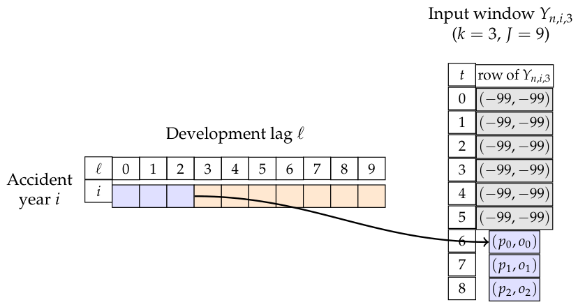
Suppose the prediction origin is $k=3$, so the model is given the history before lag 3 and is trained to predict from lag 3 onward. Because $J=9$, row t of the input window holds lag $k-J+t=t-6$ by Equation (1), so the window formally spans lags $-6,\dots ,2$. Negative lags do not exist in the triangle and are therefore padded:

$$Y_{n,i,3}=\left[\begin{array}{c}(-99,-99)\\ (-99,-99)\\ (-99,-99)\\ (-99,-99)\\ (-99,-99)\\ (-99,-99)\\ (p_0,o_0)\\ (p_1,o_1)\\ (p_2,o_2)\end{array}\right],M_{n,i,3}^x=(0,0,0,0,0,0,1,1,1).$$

The corresponding decoder target window holds lags $3,\dots ,11$. In a ten-lag triangle, lags 3 through 9 exist while lags 10 and 11 do not, so the target window and its mask are

$$\left[\begin{array}{c}(p_3,o_3)\\ (p_4,o_4)\\ (p_5,o_5)\\ (p_6,o_6)\\ (p_7,o_7)\\ (p_8,o_8)\\ (p_9,o_9)\\ (-99,-99)\\ (-99,-99)\end{array}\right],M_{n,i,3}^y=(1,1,1,1,1,1,1,0,0).$$

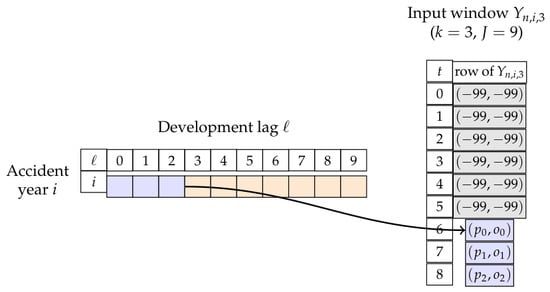
The model input uses zeros in place of the padded rows, while $M_{n,i,3}^x$ and $M_{n,i,3}^y$ record which rows are valid for the encoder update and the loss calculation, respectively. Figure 1 shows this construction schematically.

Figure 1. Construction of one $9\times 2$ input window from a paid/outstanding development triangle, using symbolic normalized values $(p_{\ell },o_{\ell })$. With prediction origin $k=3$, the window spans lags $k-J,\dots ,k-1=-6,\dots ,2$; the non-existent negative lags are padded with the sentinel $(-99,-99)$, giving input mask $(0,0,0,0,0,0,1,1,1)$. Observed history before $k=3$ is shown in blue, future target lags in orange, and non-existent (padded) lags in gray.

4.2. Three Architectures

All three architectures shared the same input processing, embedding layer, loss function, optimizer, and evaluation protocol. They differed only in the sequence processing block between the input embedding and the output heads. This controlled design ensured that performance differences were attributable to architecture alone.

• Shared components.

$\left|\mathcal{G}\right|=434$ is the number of unique group codes (NAIC entity identifier) across both lines of business. We followed the entity embedding framework of Guo and Berkhahn (2016), starting from the $\left|\mathcal{G}\right|-1$ rule but lowering the dimension to $d_e=50$ to match the scale used in Kuo (2019) and to keep the embedding dimension substantially smaller than the category cardinality, which helped prevent overfitting. The embedding was repeated across all timesteps and concatenated with the decoder output at each position before the output heads. Separate two-layer output heads produced predictions for paid losses and case reserves, each consisting of a dense layer with 64 units and ReLU activation followed by a linear projection to a scalar with ReLU to enforce non-negativity:

$$\begin{array}{cc}\hfill {\widehat{y}}_{n,i,k,t}^{\mathrm{paid}}& =\mathrm{ReLU}\left(W_2^{\mathrm{paid}}\mathrm{ReLU}(W_1^{\mathrm{paid}}{h}_{n,i,k,t}+b_1^{\mathrm{paid}})+b_2^{\mathrm{paid}}\right),\hfill \end{array}$$

(2)

$$\begin{array}{cc}\hfill {\widehat{y}}_{n,i,k,t}^{\mathrm{res}}& =\mathrm{ReLU}\left(W_2^{\mathrm{res}}\mathrm{ReLU}(W_1^{\mathrm{res}}{h}_{n,i,k,t}+b_1^{\mathrm{res}})+b_2^{\mathrm{res}}\right),\hfill \end{array}$$

(3)

where n indexes companies, i indexes accident years, k is the prediction origin, and $t=0,\dots ,J-1$ indexes relative positions in the decoder window ($J=9$); $h_{n,i,k,t}\in {\mathbb{R}}^{d_h}$ is the architecture-specific hidden state vector at decoder position t after the sequence-processing block and company embedding are combined, with $d_h=d+d_e=128+50=178$. $W_1\in {\mathbb{R}}^{64\times d_h}$ and $b_1\in {\mathbb{R}}^{64}$ are the first dense layer and bias; $W_2\in {\mathbb{R}}^{1\times 64}$ and $b_2\in \mathbb{R}$ are the output projection and scalar bias. The matrix products $W_1{h}_{n,i,k,t}$ and $W_2·\mathrm{ReLU}(·)$ contract over the feature dimension at each $(n,i,k,t)$ position to produce the scalar prediction ${\widehat{y}}_{n,i,k,t}$.

• Architecture 1: GRU Baseline.

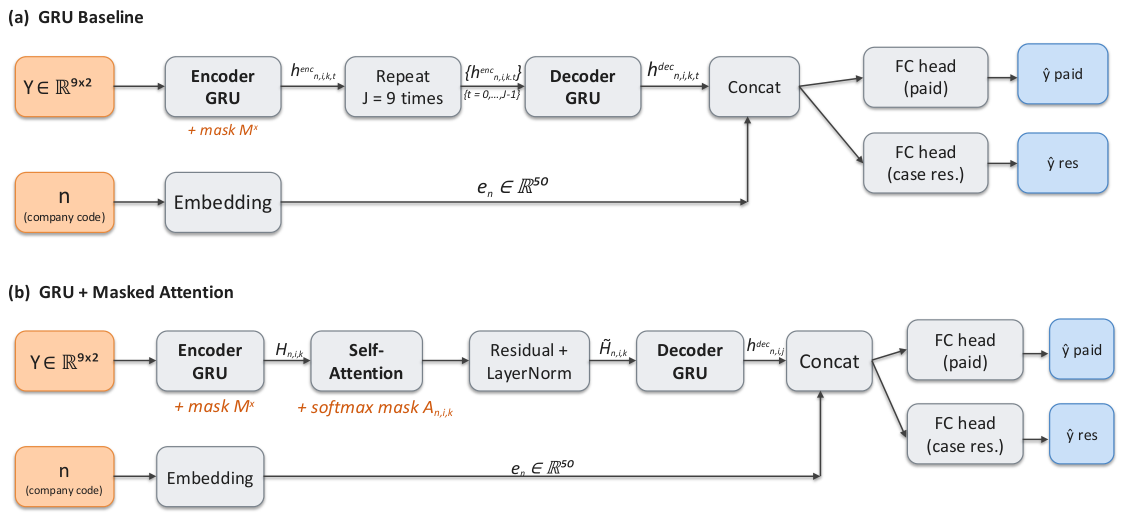
A single-layer GRU encoder with 128 hidden units processed the $9\times 2$ input matrix $Y_{n,i,k}$ row by row from $z_{n,i,k,0}$ to $z_{n,i,k,J-1}$, with the initial hidden state set to the zero vector ($h_{n,i,k,-1}^{\mathrm{enc}}=\mathbf{0}\in {\mathbb{R}}^{128}$). The encoder respected the padding mask: at each timestep, the GRU update equations below were evaluated normally, but if input position t was padded then the resulting hidden state was discarded and the previous state $h_{n,i,k,t-1}^{\mathrm{enc}}$ was carried forward unchanged. The final encoder state $h_{n,i,k,J-1}^{\mathrm{enc}}$ was repeated across all 9 timesteps and fed to a decoder GRU (also 128 units). The decoder output at each timestep was concatenated with the company embedding before being passed to the output heads (Equations (2) and (3)). The equations below describe how the GRU read one lag at a time and updated its running summary: a reset gate decided how much of the previous summary to discard, an update gate decided how much of the new candidate summary to blend in, and a padded position simply carried the previous summary forward unchanged. The encoder GRU update equations, evaluated for $t=0,1,\dots ,J-1$, were:

$$\begin{array}{cc}\hfill r_{n,i,k,t}& =\sigma (W_r[h_{n,i,k,t-1}^{\mathrm{enc}},z_{n,i,k,t}]+b_r),\hfill \end{array}$$

(4)

$$\begin{array}{cc}\hfill u_{n,i,k,t}& =\sigma (W_u[h_{n,i,k,t-1}^{\mathrm{enc}},z_{n,i,k,t}]+b_u),\hfill \end{array}$$

(5)

$$\begin{array}{cc}\hfill {\overline{h}}_{n,i,k,t}^{\mathrm{enc}}& =tanh(W_h[r_{n,i,k,t}\odot h_{n,i,k,t-1}^{\mathrm{enc}},z_{n,i,k,t}]+b_h),\hfill \end{array}$$

(6)

$$\begin{array}{cc}\hfill h_{n,i,k,t}^{\mathrm{enc}}& =u_{n,i,k,t}\odot {\overline{h}}_{n,i,k,t}^{\mathrm{enc}}+(1-u_{n,i,k,t})\odot h_{n,i,k,t-1}^{\mathrm{enc}},\hfill \end{array}$$

(7)

$$\begin{array}{cc}\hfill h_{n,i,k,t}^{\mathrm{enc}}& \leftarrow M_{n,i,k,t}^x{h}_{n,i,k,t}^{\mathrm{enc}}+(1-M_{n,i,k,t}^x)h_{n,i,k,t-1}^{\mathrm{enc}},\hfill \end{array}$$

(8)

where $r_{n,i,k,t}$ is the reset gate, $u_{n,i,k,t}$ the update gate, $\sigma (·)$ the logistic sigmoid, and ⊙ denotes elementwise (Hadamard) multiplication. Here, t indexes positions within the 9-step input window rather than absolute development lag. At the first step the recurrence consumed the first available window element against the all-zero context $h_{n,i,k,-1}^{\mathrm{enc}}=\mathbf{0}$, so $h_{n,i,k,0}^{\mathrm{enc}}=u_{n,i,k,0}\odot {\overline{h}}_{n,i,k,0}^{\mathrm{enc}}$ is the GRU state after processing the first input row rather than the input itself. Equation (8) implements the padding-aware update: when input position t is observed ($M_{n,i,k,t}^x=1$) the gated hidden state from Equation (7) is retained, whereas padded positions ($M_{n,i,k,t}^x=0$) re-use the preceding valid state.

• Architecture 2: GRU + Attention (masked).

The GRU Baseline was augmented with single-head scaled dot-product attention (Vaswani et al. 2017) applied over the encoder hidden states. We let $H_{n,i,k}=(h_{n,i,k,0}^{\mathrm{enc}},h_{n,i,k,1}^{\mathrm{enc}},\dots ,$ $h_{n,i,k,J-1}^{\mathrm{enc}})\in {\mathbb{R}}^{J\times d}$ denote the sequence of encoder states for input $Y_{n,i,k}$. Learned projection matrices $W_Q,W_K,W_V\in {\mathbb{R}}^{d\times d_k}$ with $d_k=d=128$ produced query, key, and value representations, and a learned output projection $W_O\in {\mathbb{R}}^{d_k\times d}$ with bias $b_O$ mixed the attended values back to the residual stream:

$$\begin{array}{cc}\hfill Q_{n,i,k}& =H_{n,i,k}{W}_Q,K_{n,i,k}=H_{n,i,k}{W}_K,V_{n,i,k}=H_{n,i,k}{W}_V,\hfill \end{array}$$

(9)

$$\begin{array}{cc}\hfill \mathrm{Attention}(Q_{n,i,k},K_{n,i,k},V_{n,i,k})& =\mathrm{Dropout}\left(\mathrm{softmax}\left({\displaystyle \frac{Q_{n,i,k}{K}_{n,i,k}^{\top }}{\sqrt{d_k}}}+A_{n,i,k}\right)\right)V_{n,i,k}{W}_O+b_O,\hfill \end{array}$$

(10)

where $A_{n,i,k}\in {\mathbb{R}}^{J\times J}$ is an additive attention mask with ${\left(A_{n,i,k}\right)}_{ab}=-\infty$ if key position b is padded and ${\left(A_{n,i,k}\right)}_{ab}=0$ otherwise, ensuring that the softmax assigns zero weight to unobserved positions. The dropout layer was applied to the attention weights after softmax. The attention output was combined with the original hidden states via a residual connection and layer normalization:

$${\tilde{H}}_{n,i,k}=\mathrm{LayerNorm}(H_{n,i,k}+\mathrm{Attention}(Q_{n,i,k},K_{n,i,k},V_{n,i,k})).$$

(11)

The normalized output ${\tilde{H}}_{n,i,k}$ was then fed to a decoder GRU layer (128 units), which applied the same gating mechanism of Equations (4)–(7) to produce the final hidden states, followed by the shared output heads. Note that the encoder GRU masking behavior was identical to Architecture 1—the padding mask operated via Equation (8), while the attention mask $A_{n,i,k}$ in Equation (10) operated inside the softmax. This ensured a fair comparison: both architectures saw the same encoder states, and the only difference was the addition of the attention layer. We used a single attention head to minimize parameter overhead for our short 9-timestep sequences.

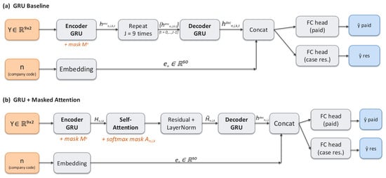
Figure 2 summarizes the implemented GRU Baseline and masked GRU + Attention architectures using the notation introduced above.

Figure 2. Implemented architectures: (a) GRU Baseline; (b) GRU + Masked Attention. The two panels share identical block geometry except in the middle: the Baseline repeats the final encoder state across $J=9$ decoder positions, while the Attention variant inserts Self-Attention followed by Residual + LayerNorm. Orange side-notes flag the input padding mask $M_{n,i,k,t}^x$ (GRU update, Equations (4)–(8)) and $A_{n,i,k}$ (softmax mask, Equation (10)). The company-code embedding $e_n\in {\mathbb{R}}^{50}$ is concatenated with the decoder output $h_{n,i,k,t}^{\mathrm{dec}}$ to form $h_{n,i,k,t}$, which feeds two ReLU-activated FC heads producing ${\widehat{y}}_{n,i,k,t}^{\mathrm{paid}}$ and ${\widehat{y}}_{n,i,k,t}^{\mathrm{res}}$ (Equations (2) and (3)). Orange = inputs, blue = outputs, gray = learned blocks.

• Architecture 3: GRU + Attention (unmasked ablation).

This variant was identical to Architecture 2 except that neither the encoder GRU nor the attention layer received a padding mask. The encoder GRU processed zero-padded positions normally (propagating hidden states through zero inputs), and the attention softmax was computed over all 9 positions regardless of validity. This variant was included solely as an ablation to test whether the masking treatment itself was responsible for any training instability in Architecture 2. We stress that this variant is not methodologically sound for production use: attending to hidden states propagated through unobserved (zero-padded) positions conflates real developmental patterns with padding artifacts.

4.3. Phase 1: Fixed Hyperparameter Comparison

We trained each of the three architecture variants (GRU Baseline, GRU + Attention masked, GRU + Attention unmasked) with a single fixed hyperparameter configuration across 50 independent random seeds, yielding 300 training runs (3 architectures × 2 LOBs × 50 seeds) and a distribution of MAPE values for each variant. Each seed initialized the PyTorch parameter random state and the NumPy data-shuffling state, so the results differed due to training stochasticity (parameter initialization, minibatch ordering, and dropout masks). The masked variant passed an explicit padding mask to both the encoder GRU and the attention layer, while the unmasked variant used neither, directly testing whether the masking treatment was responsible for any training instability in the attention variants. The pairwise comparisons used Bonferroni-corrected Welch t-tests with Cohen’s d effect sizes. The remainder of this section specifies the training protocol, evaluation metrics, and classical benchmarks used throughout Phase 1.

• Training protocol.

All three architectures were trained with identical hyperparameters in Phase 1:

• Optimizer: Adam with AMSGrad (Reddi et al. 2018), learning rate $5\times {10}^{-4}$;
• Batch size: 512;
• Maximum epochs: 1000;
• Early stopping: patience 200 epochs, minimum improvement $\delta =0.001$, monitoring validation loss;
• Dropout: a single rate of 0.10 is used throughout—as locked input and recurrent dropout inside the encoder and decoder GRU cells, as attention-weight dropout after softmax in Architectures 2–3, and between the two dense layers of each FC head.

The loss function was a masked mean squared error applied jointly to paid and case reserve predictions. The per-sample loss for company n, accident year i, and prediction origin k is:

$${\ell }_{n,i,k}={\displaystyle \frac{1}{2}}·{\displaystyle \frac{{\sum }_{t=0}^{J-1}{M}_{n,i,k,t}^y{(y_{n,i,k,t}^{\mathrm{paid}}-{\widehat{y}}_{n,i,k,t}^{\mathrm{paid}})}^2}{{\sum }_{t=0}^{J-1}{M}_{n,i,k,t}^y}}+{\displaystyle \frac{1}{2}}·{\displaystyle \frac{{\sum }_{t=0}^{J-1}{M}_{n,i,k,t}^y{(y_{n,i,k,t}^{\mathrm{res}}-{\widehat{y}}_{n,i,k,t}^{\mathrm{res}})}^2}{{\sum }_{t=0}^{J-1}{M}_{n,i,k,t}^y}},$$

(12)

where $M_{n,i,k,t}^y\in \{0,1\}$ indicates whether the decoder target at horizon position t is available. The training loss averaged over the minibatch $\mathcal{B}$: $\mathcal{L}={\displaystyle \frac{1}{\left|\mathcal{B}\right|}}{\sum }_{(n,i,k)\in \mathcal{B}}{\ell }_{n,i,k}$. All models were implemented in PyTorch 2.0+ (Paszke et al. 2019) with Python 3.9+. Hyperparameter importance analysis used scikit-learn 1.2+ (Pedregosa et al. 2011). Our experiments were conducted on an NVIDIA GB10 GPU (DGX Spark, 128 GB) and Apple M-series (Mac mini, 16 GB).

• Evaluation methodology.

The primary metric was the Mean Absolute Percentage Error (MAPE), computed per company by averaging across accident years, then averaged across all $N_{\mathrm{co}}$ companies in the test set. The predicted ultimate for company n at accident year i is:

$${\widehat{UL}}_{n,i}=C_{n,i}+{\displaystyle \sum _{m=1}^{J-j_i^{*}}}{\widehat{y}}_{n,i,k,m-1}^{\mathrm{paid}}·{\mathrm{NPE}}_{n,i},k=j_i^{*}+1,$$

(13)

where $C_{n,i}$ is the observed cumulative paid loss through the last available development lag $j_i^{*}$, k is the first unobserved development lag, ${\widehat{y}}_{n,i,k,m-1}^{\mathrm{paid}}$ is the predicted paid loss ratio for the mth future lag (Equations (2) and (3)), and ${\mathrm{NPE}}_{n,i}$ is the net premium earned. The MAPE is:

$$\mathrm{MAPE}={\displaystyle \frac{1}{N_{\mathrm{co}}}}{\displaystyle \sum _{n=1}^{N_{\mathrm{co}}}}{\displaystyle \frac{1}{|{\mathcal{I}}_n|}}\sum _{i\in {\mathcal{I}}_n}\left|{\displaystyle \frac{U{L}_{n,i}-{\widehat{UL}}_{n,i}}{U{L}_{n,i}}}\right|,$$

(14)

where $U{L}_{n,i}$ is the actual ultimate paid loss and ${\mathcal{I}}_n$ is the set of test accident years for company n. We also report the Root Mean Squared Percentage Error (RMSPE):

$$\mathrm{RMSPE}=\sqrt{{\displaystyle \frac{1}{N_{\mathrm{co}}}}\sum _{n=1}^{N_{\mathrm{co}}}{\displaystyle \frac{1}{|{\mathcal{I}}_n|}}\sum _{i\in {\mathcal{I}}_n}{\left({\displaystyle \frac{U{L}_{n,i}-{\widehat{UL}}_{n,i}}{U{L}_{n,i}}}\right)}^2}.$$

(15)

The test targets were the raw cumulative paid amounts from the triangle data, not the network’s intermediate normalized predictions, so the evaluation was anchored to observed ground truth. The test MAPE across all 50 seeds is summarized as mean ± standard deviation.

The statistical comparisons between the architectures used Bonferroni-corrected Welch t-tests. With three architecture variants, we compared each attention variant against the GRU Baseline per LOB, yielding 4 total tests and a per-test threshold of $\alpha /4=0.0125$. The Welch t-test does not assume equal variances, which is important given the substantially different standard deviations observed across the architectures. We report Cohen’s d as a measure of practical effect size:

$$d={\displaystyle \frac{{\overline{X}}_1-{\overline{X}}_2}{s_p}},s_p=\sqrt{{\displaystyle \frac{(n_1-1)s_1^2+(n_2-1)s_2^2}{n_1+n_2-2}}},$$

(16)

where ${\overline{X}}_1,{\overline{X}}_2$ are the mean MAPEs and $s_1,s_2$ the standard deviations of the two architecture groups being compared over their respective seed distributions. In our context, d quantifies how many pooled standard deviations separate the mean performance of the two architectures: $\left|d\right|<0.2$ indicates negligible practical difference, $0.5\le \left|d\right|<0.8$ a medium effect, and $\left|d\right|\ge 0.8$ a large effect (Cohen 1988). Because the attention variants had much higher variance than the Baseline (due to bimodal collapse), the pooled standard deviation was larger than either group’s alone, making the d values conservative—the performance gap would have appeared even more extreme if measured in Baseline-only standard deviation units.

If the attention MAPE distributions proved bimodal, we additionally conducted two post hoc survivor analyses per LOB, each using an uncorrected Welch t-test against the Baseline: (i) non-sentinel survivors, which excluded only runs at the exact naive-mean sentinel value; and (ii) best-converged cluster, which further restricted the surviving attention runs to the lower MAPE mode, separated from the sentinel spike by an empirical gap in which no seed fell. These post hoc filters favored attention by dropping only its worst runs without doing the same for the Baseline, providing the strongest possible case for attention. Our results are reported in Section 5.1.

• Operational definition of attention collapse.

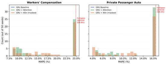
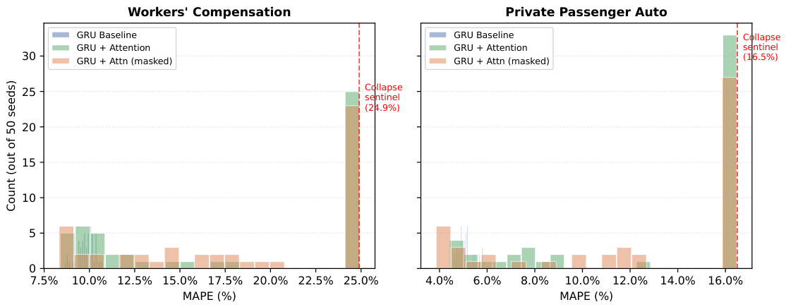
For each LOB, we made the collapse sentinel and survivor filters fully operational as follows. The sentinel was the test MAPE of a naive-mean predictor, obtained by replacing the network’s future paid-loss predictions with the training-sample mean future paid-loss ratio and then applying exactly the same normalization and test-MAPE calculation (Equations (13) and (14)) used for the neural models. Computed this way, the sentinel equaled 24.9% MAPE for Workers’ Compensation and 16.5% MAPE for Private Passenger Auto; these are the dashed lines in Figure 3. A seed was classified as collapsed when its predictions reduced to this naive-mean predictor, so that its test MAPE equaled the corresponding LOB sentinel exactly (to numerical precision) rather than merely lying near it; these seeds form the single sharp spike at the sentinel in Figure 3 (the upper mode), as distinct from the lower, converged mode. This exact-equality criterion is what produced the clean bimodal separation, since collapsed seeds piled up at one value rather than spreading across a range. The two survivor filters were then defined relative to this sentinel: the non-sentinel survivor filter removed only the seeds at the sentinel, while the best-converged cluster filter further restricted the surviving attention runs to the lower MAPE mode, which is separated from the sentinel spike by a wide gap in Figure 3 in which no seed fell (for Workers’ Compensation this lower mode contained 11 of the 50 seeds, as reported in Section 5.1). Both filters were chosen after inspecting the bimodal distributions and are therefore reported as post hoc, attention-favoring sensitivity checks rather than confirmatory tests.

Figure 3. Attention collapse bimodality (Phase 1, 50 seeds each).

• Benchmark methods.

We used three classical reserving models as benchmarks. First, Mack Chain–Ladder (CL): the standard Chain–Ladder method (Mack 1993) computes age-to-age development factors as volume-weighted averages across accident years and applies them to the latest diagonal to project ultimates. No distributional assumption is required, and Mack’s formula provides standard errors around the point estimates. Second, ODP Bootstrap: the Over-Dispersed Poisson bootstrap (England and Verrall 2002) generates a distribution of Chain–Ladder reserves by resampling Pearson residuals from the development factor model with a Poisson overdispersion correction; we used the mean of 1000 bootstrap replications as the point estimate. Third, Bornhuetter–Ferguson (BF): this method (Bornhuetter and Ferguson 1972) blends Chain–Ladder development projections with an a priori expected loss ratio, giving greater weight to the a priori for immature accident years; the expected ultimate is computed as the product of earned premium and an industry-wide expected loss ratio estimated from the training data. The BF a priori loss ratio was estimated separately by LOB as an industry-wide expected loss ratio pooled across all companies within the line, using only observations available through calendar year 2008; it is not company-specific, so every company in a given line receives the same a priori loss ratio. This pooling avoids using future test information and keeps the benchmark reproducible, but it also makes BF sensitive to how representative the pooled training-period loss ratio is for immature accident years and for individual companies whose experience differs from the industry average. All benchmark computations were completed using the chainladder-python package and used only data available through calendar year 2008 (the training cutoff) and projected to calendar year 2011, matching the neural network evaluation period.

4.4. Phase 2: Hyperparameter Sensitivity Analysis

To quantify the relative importance of hyperparameters within the GRU Baseline, we conducted a primary native Phase 2 analysis on Workers’ Compensation, and we report a native Private Passenger Auto replication in Appendix A.2. In the WC screening stage, 100 hyperparameter configurations were drawn uniformly from:

• Learning rate: log-uniform on $[{10}^{-4},5\times {10}^{-3}]$;
• Dropout rate: log-uniform on $[0.01,0.30]$;
• GRU units: uniform in $\{64,128,256\}$;
• Dense units: uniform in $\{32,64,128\}$;
• Batch size: uniform in $\{256,512,1024\}$;
• Maximum epochs: uniform in $\{500,1000\}$.

Each configuration was trained once (single seed) in the screening stage. A Random Forest regressor (Breiman 2001) was fitted to predict MAPE from the 6 hyperparameters, and its impurity-based feature importance was used as a descriptive ranking of the hyperparameters within the Phase 2 search space. In the validation stage, the top 20 configurations by screening MAPE were retrained with 5 additional independent seeds each (100 validation runs). The training, evaluation, and benchmark protocols carried over verbatim from Phase 1, except that the hyperparameter values listed above replaced the fixed Phase 1 settings.

• Additional validation.

Five supplementary analyses extended the Phase 1/Phase 2 findings and are reported in Appendix A: an attention-collapse diagnostic that showed representative loss curves and collapsed-versus-lower-mode prediction behavior (Appendix A.1); a native Private Passenger Auto Phase 2 replication that tested whether the hyperparameter-importance pattern was WC-specific (Appendix A.2); a maturity decomposition by accident year that located where the GRU Baseline gained the most over Mack CL (Appendix A.3); a consistency check against the original Kuo (2019) pipeline on a different data period (Appendix A.4); and a rolling-origin cross-validation across three temporal windows that tested whether the Baseline’s advantage was stable as the train/test boundary shifted (Appendix A.5).

5. Results

5.1. Phase 1: Fixed-HP Comparison

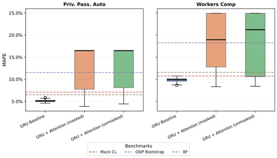
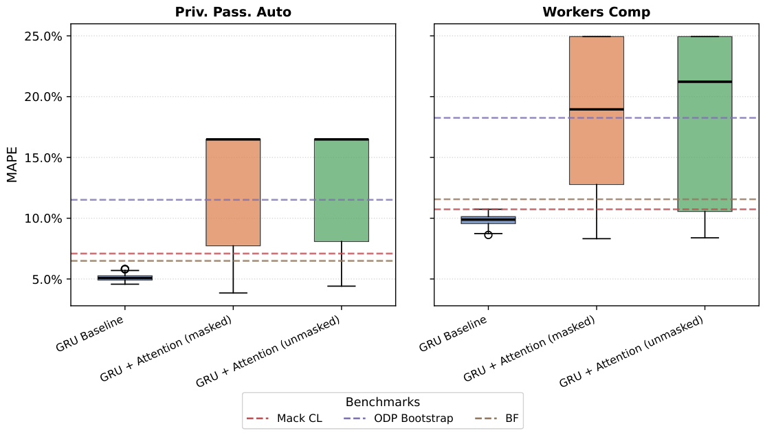
Table 2 reports our Phase 1 results across both architectures and both lines of business; Figure 4 shows the corresponding MAPE distributions over 50 seeds. The GRU Baseline had the lowest mean and median MAPE and the tightest spread in both LOBs. Figure 3 shows that both attention variants were bimodal: a cluster of converged runs at low MAPE and a second cluster sitting on the collapse sentinel (dashed line), the MAPE of the naive mean predictor. The masked and unmasked variants collapsed at similar rates, so padding mask treatment was not what drove the instability.

Table 2. Phase 1 results: MAPE and RMSPE (%) across 50 seeds under fixed hyperparameters (300 total neural network runs). Neural network results reported as mean ± std. Bold = best per column.

Method	Workers’ Compensation			Private Passenger Auto		d
	MAPE (%)	RMSPE (%)		MAPE (%)	RMSPE (%)
GRU Baseline	$\mathbf{9.82}\pm \mathbf{0.48}$	$\mathbf{19.30}\pm \mathbf{2.41}$		$\mathbf{5.13}\pm \mathbf{0.33}$	$\mathbf{9.24}\pm \mathbf{0.47}$	—
GRU + Attn. (masked)	$18.68\pm 6.46$ *	$27.83\pm 7.72$ *		$12.40\pm 4.97$ *	$20.56\pm 7.89$ *	1.94 / 2.07
GRU + Attn. (unmasked)	$18.01\pm 7.22$ *	$28.35\pm 7.68$ *		$13.24\pm 4.73$ *	$22.05\pm 7.51$ *	1.60 / 2.42
Mack CL	$10.73$	$21.56$		$7.09$	$14.89$
ODP Bootstrap	$18.25$	$27.83$		$11.51$	$20.72$
BF	$11.56$	$31.55$		$6.49$	$14.11$

d = Cohen’s d effect size vs. GRU Baseline (WC/PPA); * = $p<0.0125$ (Bonferroni-corrected, 4 tests).

Figure 4. Phase 1 MAPE distributions across 50 seeds. Boxes span the interquartile range, with black horizontal lines at the medians; circles mark outliers beyond 1.5× the interquartile range; dashed horizontal lines mark the classical benchmark MAPEs (see legend).

The dashed lines in Figure 3 mark the LOB-specific naive-mean sentinels used to tag collapsed seeds: 24.9% MAPE for Workers’ Compensation and 16.5% MAPE for Private Passenger Auto.

On Workers’ Compensation, the GRU Baseline achieved 9.82% ± 0.48% MAPE, outperforming Mack CL (10.73%), BF (11.56%), and ODP Bootstrap (18.25%). Both attention variants performed significantly worse ($p<{10}^{-10}$, $d>1.6$) and exhibited high run-to-run variance from bimodal collapse. Even after filtering out the sentinel runs, masked attention remained significantly worse than the Baseline (13.35% ± 3.79%, $p=5.3\times {10}^{-5}$); the best-converged post hoc subset was statistically indistinguishable from the Baseline but included only 11 of 50 seeds.

Private Passenger Auto showed the same pattern. The GRU Baseline achieved 5.13% ± 0.33% MAPE, outperforming Mack CL (7.09%), BF (6.49%), and ODP Bootstrap (11.51%). The masked and unmasked attention variants were significantly worse on average ($p<{10}^{-13}$ and $p<{10}^{-16}$, respectively), with 58% and 68% of seeds collapsing to the naive-mean sentinel. Filtering to non-sentinel or best-converged attention runs did not produce a statistically significant improvement over the Baseline.

Across both LOBs, the GRU Baseline improved over Mack CL by 8.5% (WC) and 27.6% (PPA) in relative MAPE, in line with the original DeepTriangle findings. Masked and unmasked attention behaved similarly, so the failure mode was not padding treatment but the limited cross-position information available on short, variable-length aggregate triangles.

5.2. Phase 2: Hyperparameter Sensitivity

Table 3 summarizes the Phase 2 screening results across 100 random hyperparameter configurations for the GRU Baseline on Workers’ Compensation. All 100 configurations converged, and the best screening MAPE (8.26%) improved on the Phase 1 fixed-hyperparameter result (9.82%) by 16%. The 6.07 pp spread between best (8.26%) and worst (14.33%) configurations was driven primarily by learning rate and regularization choices.

Table 3. Phase 2 screening: GRU Baseline MAPE (%) across 100 hyperparameter configurations (Workers’ Compensation, single seed per config).

Mean (%)	Std (%)	Best (%)	Worst (%)	Conv. Rate
$9.92\pm 1.16$	1.16	8.26	14.33	100/100

To confirm that the top-performing screening configurations were genuinely superior rather than artifacts of favorable initialization, we retrained the top 20 configurations with 5 additional seeds each (100 validation runs). Table 4 presents the top 5 validated configurations.

Table 4. Phase 2 validation: top 5 GRU Baseline configurations retrained with 6 seeds (1 screening + 5 validation). Workers’ Compensation.

Config	Mean (%)	$\mathit{\sigma }$ (%)	Screening (%)	GRU	Dropout	LR
99	8.39	0.000	8.39	256	0.015	$1.07\times {10}^{-4}$
87	8.41	0.000	8.41	128	0.042	$1.58\times {10}^{-3}$
7	8.55	0.122	8.80	256	0.025	$1.32\times {10}^{-4}$
64	8.61	0.000	8.61	256	0.020	$3.75\times {10}^{-3}$
2	8.66	0.198	8.26	256	0.034	$1.94\times {10}^{-4}$

Bold marks the best validated configuration. Standard deviations shown as $\sigma =0.000$ are rounded below the displayed three-decimal precision; the validated configurations were retrained with distinct random seeds and converged to near-identical test MAPE.

The validated top configurations were tightly clustered near 8.4–8.7% MAPE. The screening-stage winner (Config 2, screening MAPE 8.26%) dropped to rank 5 after multi-seed validation (mean 8.66%, $\sigma =0.198\%$), confirming that single-seed rankings can be misleading. The validated winner was Config 99 (mean 8.39%, $\sigma =0.000\%$), with 256 GRU units, low dropout (1.5%), and a conservative learning rate ($1.07\times {10}^{-4}$). Config 99 improved over the Phase 1 fixed-hyperparameter result (9.82%) by 14.5% and over Mack Chain–Ladder (10.73%) by 21.8%. The configurations reported with $\sigma =0.000$ were not literally identical across seeds: each validation run used a distinct random seed and a fresh initialization, but after early stopping on validation loss the runs converged to test MAPEs that differed only below the three-decimal precision shown here, on the small single-diagonal test set.

• Feature importance.

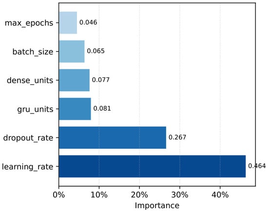
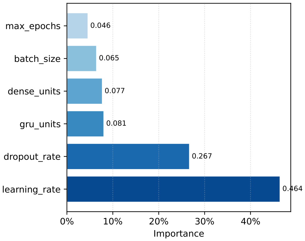
A Random Forest regressor (Breiman 2001) fitted to the 100 screening configurations summarized each hyperparameter’s contribution to MAPE using impurity-based feature importance. Figure 5 shows that learning rate (46.4%) and dropout rate (26.7%) were the two dominant features, together accounting for over 73% of the impurity-based feature importance.

Figure 5. Random Forest feature importance for predicting GRU Baseline MAPE from hyperparameters (Phase 2, 100 configurations).

The remaining four hyperparameters—GRU units (8.1%), dense units (7.7%), batch size (6.5%), and max epochs (4.6%)—together accounted for less than 27% of the impurity-based importance. Doubling the GRU units from 128 to 256, which doubled the recurrent parameter count, received less than one-fifth of the importance attributed to learning rate. Tuning the optimizer and regularization settings mattered more than searching over hidden dimensions.

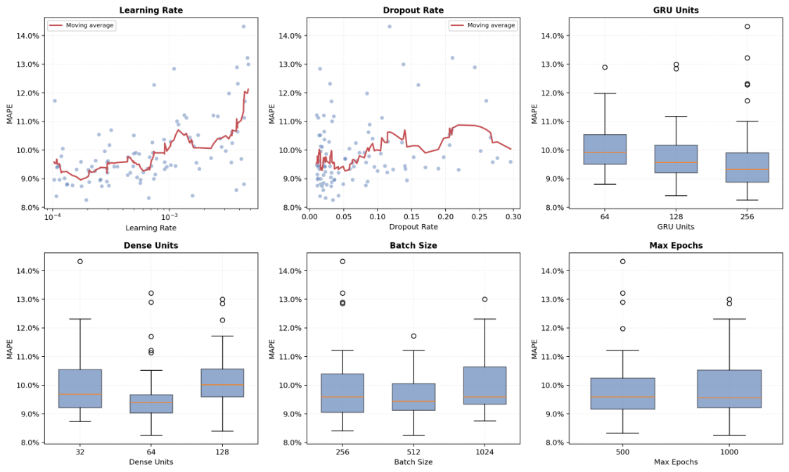
These feature-importance values should be read as a descriptive decomposition from the fitted Random Forest surrogate, not as causal effects of the hyperparameters. Impurity-based Random Forest importance is known to favor continuous or high-cardinality predictors, because they offer more candidate split points. In our design, learning rate and dropout are continuous (drawn log-uniformly), whereas GRU units, dense units, batch size, and maximum epochs are discrete with at most three levels, so the importance assigned to the two continuous hyperparameters is not directly comparable to a randomized causal effect and may depend on the six-dimensional search space used in Phase 2. To check whether this split-point bias drove the ranking, we also computed permutation importance on the fitted Random Forest surrogate. The top-two ranking was unchanged: learning rate and dropout accounted for 36.0% and 22.0% of the normalized permutation-importance decrease on Workers’ Compensation and for 38.3% and 19.3% on Private Passenger Auto. The conclusion does not, however, rest on impurity scores alone: the observed-configuration scatter and boxplots in Figure 6 are model-free and corroborate the ranking, with the strongest MAPE gradients appearing along learning rate and dropout, and much flatter relationships for the hidden widths, batch size, and maximum epochs. We therefore interpret learning rate and dropout as the dominant hyperparameters within this experiment’s search design rather than as universal causal drivers of reserving accuracy.

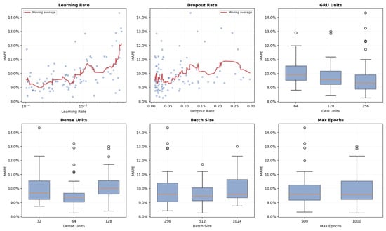
Figure 6. Observed-configuration view of Phase 2 hyperparameter sensitivity for the GRU Baseline on Workers’ Compensation: scatter with a moving-average line for the two continuous hyperparameters (learning rate, dropout) and boxplots for the four discrete hyperparameters (GRU units, dense units, batch size, max epochs), plotted directly from the 100 screening runs. In the two scatter panels, the orange curve is the moving-average line; in the boxplots, orange horizontal lines mark the medians and circles mark outliers beyond 1.5× the interquartile range.

Figure 6 shows the relationship between the hyperparameters and the model performance. The first panel shows the learning rate–MAPE relationship across all 100 configurations with degradation pattern above the optimal region [${10}^{-4},{10}^{-3}$]. The best configurations clustered in a narrow band around ${10}^{-4}$, and even moderately suboptimal learning rates ($>{10}^{-3}$) yielded MAPEs below 12%—further evidence that the GRU Baseline’s loss landscape was well-behaved. The second dropout panel shows best performance at low dropout ($<5\%$) and degradation under aggressive regularization ($>10\%$). The combination of low learning rate and low dropout characterizes all of the top-performing configurations in Table 4. The remaining panels reinforce the Random Forest ranking: GRU width, dense width, batch size, and max epochs moved performance much less than optimizer and regularization choices.

• Hyperparameters vs. architecture.

The dominant Phase 2 finding is that the ranking of hyperparameter importance is stable across business lines, even though the optimal values are not. On Workers’ Compensation, the GRU Baseline averaged 9.92% ± 1.16% MAPE across 100 screening configurations, with a validated best of 8.39% (Config 99). The spread between good and poor configurations was large enough to matter actuarially, so tuning a simple GRU Baseline is not a minor implementation detail.

Appendix A reports the attention-collapse diagnostic and four supplementary validation analyses. A consistency check against the original Kuo (2019) protocol on a 50-company subset shows that our re-implementation reproduced the structural behavior of DeepTriangle on a different data period, including the qualitative effect of ensembling. A maturity decomposition by accident year shows that the GRU Baseline’s absolute gain over Mack CL was largest on immature accident years, where Chain–Ladder development factors were most uncertain. A rolling-origin cross-validation across three temporal windows showed that the Baseline’s advantage over Mack CL held across evaluation periods and that MAPE improved as more training data became available.

6. Discussion

6.1. Why Does Attention Underperform?

The most parsimonious explanation is structural. Aggregate triangles contain at most 9 development lags per company, and the GRU encoder already summarizes this short sequence into a fixed-length hidden state before attention is applied. In longer sequences, such as individual claim trajectories or natural language, attention helps by letting distant positions interact directly. On 9-lag triangles, the recurrent “bottleneck” is not actually a bottleneck; the attention layer mostly adds parameters and optimization variance without adding cross-position information the GRU does not already carry. The masked and unmasked variants collapse at similar rates, which fits this explanation better than a masking bug.

We also tested multi-head attention, temperature annealing, and identity initialization of $W_Q,W_K$ on top of the standard scaled dot-product attention with residual connection, layer normalization, and dropout (7 variants, 140 additional runs). None improved convergence above the single-head baseline. These failures do not rule out attention for richer actuarial sequences, but they make it a poor default for aggregate triangles of this length.

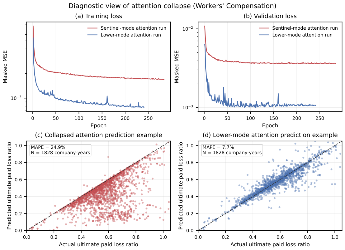
Under the test-MAPE calculation, a collapsed attention run produced ultimate-loss predictions equivalent to replacing the model’s future paid-loss sequence with the naive-mean future paid-loss pattern, yielding 24.9% MAPE on Workers’ Compensation and 16.5% on Private Passenger Auto—the sentinel values of Figure 3. These sit far above the corresponding GRU Baseline means of 9.82% and 5.13%. The failure is therefore not a small loss of efficiency but a qualitatively different predictive regime, in which the fitted network stops using the company- and accident-year-specific development history in any useful way and reverts to an almost constant average prediction. Appendix A Figure A1 illustrates this distinction with representative attention loss curves and actual-versus-predicted ultimate paid-loss ratios for collapsed and lower-mode attention examples; the lower-mode example is illustrative and does not change the distributional conclusion that attention is not a reliable improvement over the GRU Baseline on these short aggregate triangles.

6.2. Practical Implications

The findings imply a clear order of operations for neural network aggregate reserving. The GRU Baseline is a sensible starting point, in line with the CANN literature’s finding that simple structures augmented by neural networks often outperform more complex alternatives when the added complexity does not introduce a new signal (Gabrielli et al. 2020; Wüthrich and Merz 2019). With the architecture fixed, learning rate and dropout should be tuned first: in the Phase 2 Random Forest surrogate these two hyperparameters together received about three-quarters of the impurity-based importance in both the WC and the native PPA sweeps, while recurrent width, dense width, batch size, and maximum epochs were secondary within the tested search space. The best values differed materially across the LOBs, so hyperparameters should be tuned per business line.

The results should be read as point-prediction results, not as a complete reserve-uncertainty framework. MAPE and RMSPE are useful for comparing predictive accuracy under a matched protocol, but production reserving also requires uncertainty ranges, sensitivity testing, and actuarial judgment around aggregate reserve risk. Classical methods remain useful here: Mack Chain–Ladder supplies standard errors around the Chain–Ladder estimate, and the ODP bootstrap supplies a predictive distribution through residual resampling. Neural-network ensembles can also reduce point-estimate variance—in our Kuo replication, ensembling 10–20 models lowered MAPE from 9.13% to 8.32%—and the dispersion across ensemble members can serve as a rough, diagnostic indicator of model stability. This dispersion is at most an implicit uncertainty proxy and should not be treated as a calibrated reserve distribution without additional validation.

For production use, the practical question is not whether a percentage-point improvement looks large in a table, but whether it is material relative to the premium volume and reserve risk of the portfolio. In Phase 1 the GRU Baseline improved on Mack Chain–Ladder by 0.91 pp on Workers’ Compensation (9.82% vs. 10.73%) and by 1.96 pp on Private Passenger Auto (5.13% vs. 7.09%); after tuning, the best validated WC configuration (Config 99) improved on Mack by 2.34 pp (8.39% vs. 10.73%). For large portfolios, differences of this order can be economically meaningful, but they should be evaluated at the aggregate-reserve level and by maturity, not only through average company-level MAPE. The maturity analysis in Appendix A.3 shows that the absolute gain over Mack concentrated on immature accident years (2.12 pp versus 0.50 pp on mature years), where Chain–Ladder development factors were sparsest and most influential on the ultimate estimate, while mature years showed smaller absolute differences.

The appropriate workflow is therefore conservative. A reserving actuary should first require the neural model to beat a well-implemented Mack Chain–Ladder benchmark under the same valuation date and test diagonal; 10 seeds is a reasonable minimum for architecture selection and 50 seeds for publication-quality comparisons. If the neural model does not beat Mack, the first remedy should be tuning the GRU Baseline rather than adding architectural complexity. Once point accuracy is adequate, explicit uncertainty quantification should be added: candidate extensions include mixture density networks for predictive distributions (Al-Mudafer et al. 2022), conformal prediction for empirical prediction intervals, and diffusion-based generative reserving models (Gao et al. 2026). These are natural future directions but lie outside the point-prediction comparison studied here.

• Reproducibility on public Schedule P data.

The proprietary data restriction prevents exact numerical replication of the reported MAPE values, collapse rates, and selected hyperparameters. The publicly available CAS Loss Reserve Database has the same Schedule P structure and can be used to reproduce the methodological pipeline: construction of normalized paid/outstanding windows, GRU Baseline and attention-variant training, temporal splits adapted to the public data period, classical benchmark construction, and the hyperparameter screening protocol. On the public data the replication target is qualitative rather than exact—whether a tuned GRU Baseline remains competitive with Mack Chain–Ladder, whether attention adds accuracy or instability on short aggregate triangles, and whether learning rate and dropout dominate hidden-width choices within a comparable search design—rather than reproduction of the exact performance levels and collapse frequencies, which depend on the proprietary panel.

7. Conclusions

Across more than 700 training runs on two lines of business, adding attention did not improve neural network loss reserving on aggregate triangles. The GRU Baseline outperformed both attention variants, which suffered from a bimodal training instability on sequences too short for attention to add useful cross-position information.

Native Phase 2 sweeps on both WC and PPA showed the same pattern: MAPE was highly sensitive to learning rate and dropout, but the best values differed by LOB. The practical implication is to tune a simple GRU Baseline separately for each line of business before considering more complex architectures.

These findings apply to short aggregate triangles. Individual-claim models with longer sequences, richer covariates, or multi-line dependencies may still benefit from attention. Extending the analysis to predictive distributions—through mixture density networks (Al-Mudafer et al. 2022), conformal prediction, or diffusion-based generative models (Gao et al. 2026)—and to full transformer architectures remains open work.

Appendix A.1. Attention-Collapse Diagnostic

Figure A1 adds the requested diagnostic view of the attention-collapse failure mode. The top panels show the representative attention training and validation loss curves from the Workers’ Compensation runs that ended in the sentinel mode versus the lower MAPE mode. The sentinel-mode curve continued to optimize the training objective but plateaued at a substantially worse validation loss, consistent with the model learning a weak average-development pattern rather than company- and accident-year-specific structure. The bottom panels show the practical effect on ultimate-loss predictions: the collapsed attention example remained at the 24.9% sentinel and systematically underpredicted high actual ultimate paid-loss ratios, while a lower-mode attention example tracked the diagonal much more closely (7.7% MAPE). This lower-mode panel is an illustrative example of the lower cluster rather than evidence of a reliable attention advantage; the primary Phase 1 conclusion is based on the full seed distribution in Table 2 and Figure 3, where attention was worse on average and any post hoc survivor subset was not a stable architectural improvement.

Figure A1. Diagnostic view of attention collapse on Workers’ Compensation. Panels (a,b) show representative attention training and validation loss curves for a sentinel-mode run and a lower-mode run. Panels (c,d) compare actual versus predicted ultimate paid-loss ratios for collapsed and lower-mode attention prediction examples; the dashed line is perfect prediction. The lower-mode panel illustrates that non-collapsed attention can fit the target well in selected runs, but the distributional comparison in Table 2 and Figure 3 shows that this behavior is not reliable across seeds.

Figure A1. Diagnostic view of attention collapse on Workers’ Compensation. Panels (a,b) show representative attention training and validation loss curves for a sentinel-mode run and a lower-mode run. Panels (c,d) compare actual versus predicted ultimate paid-loss ratios for collapsed and lower-mode attention prediction examples; the dashed line is perfect prediction. The lower-mode panel illustrates that non-collapsed attention can fit the target well in selected runs, but the distributional comparison in Table 2 and Figure 3 shows that this behavior is not reliable across seeds.

Appendix A.2. Native PPA Phase 2 Replication

To test whether the Phase 2 hyperparameter-sensitivity pattern was specific to Workers’ Compensation, we repeated the GRU Baseline protocol natively on Private Passenger Auto. The design matched the WC sweep: 100 random configurations were trained once for screening, and the top 20 were retrained with 5 additional independent seeds each. Table A1 summarizes the PPA screening distribution and the top validated configurations. These results are reported as a qualitative replication of the importance ranking, not as evidence that WC-selected hyperparameters transfer to PPA.

Table A1. Native PPA Phase 2 replication: screening summary and top validated GRU Baseline configurations. Screening used 100 configurations with one seed each; validation retrained the top 20 configurations with 5 additional seeds each.

Panel	Config	Mean MAPE (%)	$\mathit{\sigma }$ (%)	LR	Dropout	GRU
Screening distribution	—	5.55	2.81	—	—	—
Validated top 1	48	1.91	0.000	$4.76\times {10}^{-3}$	0.138	128
Validated top 2	54	1.94	0.000	$1.10\times {10}^{-3}$	0.015	128
Validated top 3	49	1.95	0.000	$4.13\times {10}^{-3}$	0.052	64
Validated top 4	11	1.95	0.000	$2.61\times {10}^{-3}$	0.035	128
Validated top 5	67	2.01	0.000	$1.13\times {10}^{-3}$	0.110	128

Bold marks the best validated configuration. Standard deviations shown as $\sigma =0.000$ are rounded below the displayed three-decimal precision; the validated configurations were retrained with distinct random seeds and converged to near-identical test MAPE.

Table A1. Native PPA Phase 2 replication: screening summary and top validated GRU Baseline configurations. Screening used 100 configurations with one seed each; validation retrained the top 20 configurations with 5 additional seeds each.

Panel	Config	Mean MAPE (%)	$\mathit{\sigma }$ (%)	LR	Dropout	GRU
Screening distribution	—	5.55	2.81	—	—	—
Validated top 1	48	1.91	0.000	$4.76\times {10}^{-3}$	0.138	128
Validated top 2	54	1.94	0.000	$1.10\times {10}^{-3}$	0.015	128
Validated top 3	49	1.95	0.000	$4.13\times {10}^{-3}$	0.052	64
Validated top 4	11	1.95	0.000	$2.61\times {10}^{-3}$	0.035	128
Validated top 5	67	2.01	0.000	$1.13\times {10}^{-3}$	0.110	128

Bold marks the best validated configuration. Standard deviations shown as $\sigma =0.000$ are rounded below the displayed three-decimal precision; the validated configurations were retrained with distinct random seeds and converged to near-identical test MAPE.

The qualitative importance pattern mirrored Workers’ Compensation. In the PPA Random Forest importance model, learning rate received 46.9% of the impurity-based importance and dropout 25.3%, compared with 46.4% and 26.7% in WC. The remaining features were secondary on both LOBs: batch size (8.4% PPA vs. 6.5% WC), GRU units (8.1% vs. 8.1%), dense units (7.1% vs. 7.7%), and max epochs (4.2% vs. 4.6%). The optimal hyperparameter levels, however, were LOB-specific: the best validated PPA configurations used higher learning rates and higher dropout than the WC winner. The replication therefore supports the importance ranking, not cross-LOB transfer of selected hyperparameters.

Appendix A.3. Maturity Analysis

We decomposed test performance by accident year maturity to understand when neural networks provided the greatest advantage over classical methods. Accident years 2002–2006 (5–9 development lags observed) were classified as “mature”; accident years 2007–2010 (1–4 lags observed) as “immature.” Table A2 presents the maturity-stratified MAPE for all methods on Workers’ Compensation at seed $=0$.

Table A2. Maturity-stratified MAPE (%) for Workers’ Compensation (seed $=0$). Mature = accident years 2002–2006; Immature = accident years 2007–2010.

Method	Overall (%)	Mature AY 2002–2006 (%)	Immature AY 2007–2010 (%)
GRU Baseline	8.56	3.21	12.19
GRU + Attention	8.40	3.40	12.06
Mack CL	10.73	3.71	14.31
GRU Baseline improvement over Mack (pp)	$-2.17$	$-0.50$	$-2.12$

The italicized row is a derived quantity—the GRU Baseline’s improvement over Mack CL in percentage points—rather than a separate method.

Table A2. Maturity-stratified MAPE (%) for Workers’ Compensation (seed $=0$). Mature = accident years 2002–2006; Immature = accident years 2007–2010.

Method	Overall (%)	Mature AY 2002–2006 (%)	Immature AY 2007–2010 (%)
GRU Baseline	8.56	3.21	12.19
GRU + Attention	8.40	3.40	12.06
Mack CL	10.73	3.71	14.31
GRU Baseline improvement over Mack (pp)	$-2.17$	$-0.50$	$-2.12$

The italicized row is a derived quantity—the GRU Baseline’s improvement over Mack CL in percentage points—rather than a separate method.

The relative MAPE improvement of the GRU Baseline over Mack CL was similar in the mature and immature buckets (about 13% and 15%), but the absolute improvement was much larger on immature accident years: 2.12 percentage points (12.19% vs. 14.31%) versus only 0.50 percentage points (3.21% vs. 3.71%) on mature years. Within the GRU per-lag breakdown, MAPE rose sharply with immaturity: from 1.07% at lag 9 (AY 2002) to 5.53% at lag 5 (AY 2006) to 19.26% at lag 1 (AY 2010). The Baseline’s absolute gain over Mack therefore concentrated on accident years 2007–2010, where Chain–Ladder development factors were sparsest and most influential on the ultimate estimate. On accident years 2002–2006, where 5–9 development years were already observed, both methods performed comparably (Mack 3.71% vs. GRU 3.21%), since at high maturity the Chain–Ladder factors had stabilized and the neural network’s cross-company pooling added little.

Appendix A.4. Consistency with Kuo (2019)

To check that our pipeline reproduced the qualitative behavior of the original DeepTriangle, we trained a 20-model GRU Baseline ensemble on a 50-company Workers’ Compensation subsample drawn from our data, mirroring Kuo’s ensemble protocol. Absolute MAPE values were not comparable across studies because our data covered accident years 2002–2010 and a different company panel than Kuo’s 1988–1997 subset, so we looked for two structural signals instead. First, ensembling produced the same qualitative gain Kuo reported: averaging predictions from 20 models reduced test MAPE from a single-seed mean of 9.13% to 8.32%, an 8.9% relative improvement that mirrored the direction and rough magnitude of the gain Kuo attributed to ensembling. Second, increasing the batch size from our default 512 to Kuo’s 2250 modestly degraded the ensemble (8.32% → 9.26%), consistent with the Phase 2 finding that the optimal batch size depended on the dataset. Together with the Phase 1 result that the single-seed GRU Baseline beat Mack on the full WC panel (9.82% vs. 10.73%, an 8.5% relative improvement), this confirms that our re-implementation reproduced the structural behavior of DeepTriangle on a different evaluation window, even though the company-subset Mack benchmark on these 50 companies was not directly comparable to either Kuo’s or our full-panel results.

Appendix A.5. Temporal Robustness

The Phase 1 results were based on a single temporal window: training data through calendar year 2008, with the 2011 diagonal as the test set. To assess whether the GRU Baseline’s advantage was robust across evaluation periods, we conducted a rolling-origin cross-validation study using three temporal windows on Workers’ Compensation:

• W1: train $\le 2006$, validation 2007–2008, test diagonal 2009;
• W2: train $\le 2007$, validation 2008–2009, test diagonal 2010;
• W3: train $\le 2008$, validation 2009–2010, test diagonal 2011 (Phase 1 setup).

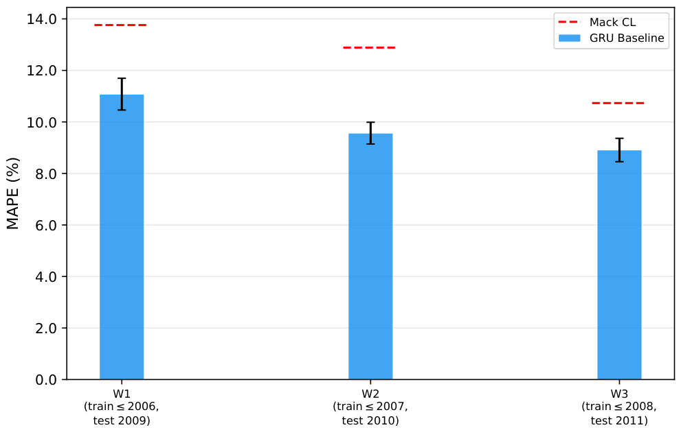
Each window shifted the entire train/validation/test boundary by one year. We trained the GRU Baseline with 10 independent seeds per window under the same fixed hyperparameters as Phase 1. The Mack Chain–Ladder benchmarks were recomputed for each window. Table A3 presents the results; Figure A2 shows the grouped bar chart with the Mack CL benchmarks.

Table A3. Temporal robustness: GRU Baseline MAPE (%) across 10 seeds per window (Workers’ Compensation, fixed hyperparameters). Mack CL benchmark recomputed per window.

Window	Train≤	GRU Baseline	Mack CL	Relative Improvement
W1	2006	$11.08\pm 0.62$ (10/10)	$13.76$	$-19.5\%$
W2	2007	$9.57\pm 0.42$ (10/10)	$12.89$	$-25.8\%$
W3	2008	$8.91\pm 0.45$ (10/10)	$10.73$	$-16.9\%$

Parentheses = convergence rate (seeds with MAPE $<20\%$/total).

Table A3. Temporal robustness: GRU Baseline MAPE (%) across 10 seeds per window (Workers’ Compensation, fixed hyperparameters). Mack CL benchmark recomputed per window.

Window	Train≤	GRU Baseline	Mack CL	Relative Improvement
W1	2006	$11.08\pm 0.62$ (10/10)	$13.76$	$-19.5\%$
W2	2007	$9.57\pm 0.42$ (10/10)	$12.89$	$-25.8\%$
W3	2008	$8.91\pm 0.45$ (10/10)	$10.73$	$-16.9\%$

Parentheses = convergence rate (seeds with MAPE $<20\%$/total).

The GRU Baseline beat Mack CL in every window with 100% convergence. MAPE decreased monotonically from W1 to W3 as more training data became available: 11.08% (W1, train $\le 2006$) to 8.91% (W3, train $\le 2008$), a 19.6% relative improvement from two additional years of training data. The Baseline’s relative improvement over Mack CL was consistent across windows, ranging from 16.9% (W3) to 25.8% (W2). The Phase 1 findings were not artifacts of a single evaluation period.

Figure A2. Temporal robustness of GRU Baseline across three rolling windows. The GRU Baseline (blue) beat the Mack CL benchmark (red dashed) in all windows with 100% convergence. MAPE improved monotonically as more training data became available.

Figure A2. Temporal robustness of GRU Baseline across three rolling windows. The GRU Baseline (blue) beat the Mack CL benchmark (red dashed) in all windows with 100% convergence. MAPE improved monotonically as more training data became available.

References

- Al-Mudafer, Muhammed Taher, Benjamin Avanzi, Greg Taylor, and Bernard Wong. 2022. Stochastic loss reserving with mixture density neural networks. Insurance: Mathematics and Economics 105: 144–74. [Google Scholar] [CrossRef] [Scilit]
- Bornhuetter, Ronald L., and Ronald E. Ferguson. 1972. The actuary and IBNR. Proceedings of the Casualty Actuarial Society 59: 181–95. [Google Scholar]
- Brauer, Alexej. 2024. Enhancing actuarial non-life pricing models via transformers. European Actuarial Journal 14: 287–315. [Google Scholar] [CrossRef] [Scilit]
- Breiman, Leo. 2001. Random forests. Machine Learning 45: 5–32. [Google Scholar] [CrossRef] [Scilit]
- Cai, Pengfei, Anas Abdallah, and Pratheepa Jeganathan. 2026. Recurrent neural networks for multivariate loss reserving and risk capital analysis. North American Actuarial Journal 30: 381–405. [Google Scholar] [CrossRef] [Scilit]
- Chaoubi, Ihsan, Camille Besse, Hélène Cossette, and Marie-Pier Côté. 2023. Micro-level reserving for general insurance claims using a long short-term memory network. Applied Stochastic Models in Business and Industry 39: 382–407. [Google Scholar] [CrossRef] [Scilit]
- Cohen, Jacob. 1988. Statistical Power Analysis for the Behavioral Sciences, 2nd ed. Hillsdale: Lawrence Erlbaum Associates. [Google Scholar]
- England, Peter D., and Richard J. Verrall. 2002. Stochastic claims reserving in general insurance. British Actuarial Journal 8: 443–518. [Google Scholar] [CrossRef] [Scilit]
- Feng, Yining, and Shuanming Li. 2024. Advancing the use of deep learning in loss reserving: A generalized DeepTriangle approach. Risks 12: 4. [Google Scholar]
- Gabrielli, Andrea. 2021. An individual claims reserving model for reported claims. European Actuarial Journal 11: 541–77. [Google Scholar] [CrossRef] [Scilit]
- Gabrielli, Andrea, Ronald Richman, and Mario V. Wüthrich. 2020. Neural network embedding of the over-dispersed Poisson reserving model. Scandinavian Actuarial Journal 2020: 1–29. [Google Scholar] [CrossRef] [Scilit]
- Gao, Shiying, Yuning Zhang, Ruikun Li, S. T. Boris Choy, and Junbin Gao. 2026. Probabilistic loss reserving prediction via denoising diffusion model. Insurance: Mathematics and Economics 127: 45–68. [Google Scholar] [CrossRef] [Scilit]
- Guo, Cheng, and Felix Berkhahn. 2016. Entity embeddings of categorical variables. arXiv arXiv:1604.06737. [Google Scholar]
- Kuo, Kevin. 2019. DeepTriangle: A deep learning approach to loss reserving. Risks 7: 97. [Google Scholar] [CrossRef] [Scilit]
- Mack, Thomas. 1993. Distribution-free calculation of the standard error of chain-ladder reserve estimates. ASTIN Bulletin 23: 213–25. [Google Scholar] [CrossRef] [Scilit]
- Paszke, Adam, Sam Gross, Francisco Massa, Adam Lerer, James Bradbury, Gregory Chanan, Trevor Killeen, Zeming Lin, Natalia Gimelshein, Luca Antiga, and et al. 2019. PyTorch: An imperative style, high-performance deep learning library. In Advances in Neural Information Processing Systems 32. Red Hook: Curran Associates, Inc., pp. 8024–35. [Google Scholar]
- Pedregosa, Fabian, Gaël Varoquaux, Alexandre Gramfort, Vincent Michel, Bertrand Thirion, Olivier Grisel, Mathieu Blondel, Peter Prettenhofer, Ron Weiss, Vincent Dubourg, and et al. 2011. Scikit-learn: Machine learning in Python. Journal of Machine Learning Research 12: 2825–30. [Google Scholar]
- Reddi, Sashank J., Satyen Kale, and Sanjiv Kumar. 2018. On the convergence of Adam and beyond. 6th International Conference on Learning Representations, Vancouver, BC, Canada, April 30–May 3. [Google Scholar]
- Richman, Ronald. 2026. Scaling laws, tabular data, and actuarial ratemaking models. SSRN, preprint (posted 11 January 2026).
- Schneider, Judith C., and Brandon Schwab. 2025. Advancing loss reserving: A hybrid neural network approach for individual claim development prediction. Journal of Risk and Insurance 92: 389–423. [Google Scholar]
- Vaswani, Ashish, Noam Shazeer, Niki Parmar, Jakob Uszkoreit, Llion Jones, Aidan N. Gomez, Łukasz Kaiser, and Illia Polosukhin. 2017. Attention is all you need. 31st International Conference on Neural Information Processing Systems, Long Beach, CA, USA, December 4–9; pp. 5998–6008. [Google Scholar]
- Wüthrich, Mario V. 2018a. Machine learning in individual claims reserving. Scandinavian Actuarial Journal 2018: 465–80. [Google Scholar] [CrossRef] [Scilit]
- Wüthrich, Mario V. 2018b. Neural networks applied to chain-ladder reserving. European Actuarial Journal 8: 407–36. [Google Scholar] [CrossRef] [Scilit]
- Wüthrich, Mario V., and Michael Merz. 2019. Editorial: Yes, we CANN! ASTIN Bulletin 49: 1–3. [Google Scholar]
Disclaimer/Publisher’s Note: The statements, opinions and data contained in all publications are solely those of the individual author(s) and contributor(s) and not of MDPI and/or the editor(s). MDPI and/or the editor(s) disclaim responsibility for any injury to people or property resulting from any ideas, methods, instructions or products referred to in the content. |
© 2026 by the author. Licensee MDPI, Basel, Switzerland. This article is an open access article distributed under the terms and conditions of the Creative Commons Attribution (CC BY) license.