


Highlights
What are the main findings?
- Routinely available clinical and laboratory data identified prevalent dysglycaemia with an area under the curve of 0.810 internally and 0.818 in a later, independently collected survey cycle. In the development cycle, the only cycle in which the questionnaire could be scored, the model exceeded the published American Diabetes Association risk test by 0.0694 (95% CI 0.0493 to 0.0906).
- Refitting the questionnaire’s own items in this population accounted for about one-fifth of that advantage; the remainder was the net effect of replacing those items with routine measurements. Gradient boosting did not improve on a penalised logistic regression.
What are the implications of the main findings?
- Where a metabolic panel and a complete blood count are already on file, the decision about whom to test can be made from those data rather than from a self-administered questionnaire, detecting 10.6 more percentage points of cases at the same specificity (95% CI 5.9 to 15.0).
- Because a transparent regression matched the gradient-boosting models, the deployable product of this line of work is a published equation rather than a model artefact.
Abstract
Background/Objectives: Whom to test for dysglycaemia is usually decided with a questionnaire, even when routine blood results are on file. We asked whether routine clinical data identify prevalent dysglycaemia better than the American Diabetes Association (ADA) risk test, how much of any advantage reflects refitting its items, and whether machine learning was needed. Methods: A model was developed in NHANES adults aged 20 years or older without diagnosed diabetes (2017–March 2020, n = 6649) and validated in the held-back August 2021–August 2023 cycle (n = 4826). The outcome was HbA1c 5.7% or higher. Forty-eight predictors from an encounter with a metabolic panel and a complete blood count were used; no glycaemic measurement entered any model. Penalised logistic regression, LightGBM, XGBoost, and the ADA risk test were compared by nested cross-validation. Performance estimates used survey weights, with confidence intervals from a bootstrap of primary sampling units within strata. Results: The regression reached an area under the curve of 0.810 (95% CI 0.788 to 0.830) internally and 0.818 (0.799 to 0.835) in the validation cycle, with calibration slopes of 1.04 and 1.08. Neither gradient-boosting model improved on it. In the development cycle, where the questionnaire could be scored, the regression exceeded it by 0.0694 (0.0493 to 0.0906; p < 0.001); refitting the ADA items accounted for 0.0150, and the remaining 0.0544 reflected adding 44 measurements and omitting three questionnaire items. At the questionnaire’s specificity, the model detected 10.6 more percentage points of cases (5.9 to 15.0). Conclusions: Among adults with a metabolic panel and a complete blood count on file, routine clinical data identified dysglycaemia better than the ADA questionnaire, and performance was reproduced in a later cycle. A transparent regression matched gradient boosting; most of the advantage came from the change in predictor set rather than from refitting the questionnaire’s items.
1. Introduction
Dysglycaemia, prediabetes, or diabetes that has not yet been diagnosed is common, largely asymptomatic, and consequential. Between 1999 and 2018, the age-standardised prevalence of prediabetes among United States adults rose from 29.5% to 48.3%, while undiagnosed diabetes remained stable at about 3% of adults [1]. Both the prevalence of dysglycaemia and the proportion that remains undiagnosed differ across sociodemographic groups in the United States [1], so the equity of any rule that decides whom to test is a relevant consideration. Because progression to diabetes can be slowed by lifestyle and pharmacological intervention, and because the interventions work best early, guidelines recommend screening all adults from the age of 35 years and younger adults who carry risk factors [2].
The recommendation is easier to state than to implement. Testing every adult every three years is a large volume of laboratory work, so in practice clinicians decide whom to test, and the tools available to support that decision are questionnaires. The ADA risk test comprises seven items (age, sex, history of gestational diabetes, family history of diabetes, history of high blood pressure, physical activity, and a body-mass-index band) and returns a score with a recommended action threshold of 5 [3]. The Finnish Diabetes Risk Score [4] and other non-invasive scores [5,6] rest on the same principle, and their discrimination for prevalent or incident dysglycaemia is typically in the range of 0.70 to 0.80 across populations [7,8,9]. The Finnish score has also been examined for outcomes beyond glycaemia; in a Turkish primary-care sample, it was independently associated with the fibrosis-4 index [10].
Questionnaire scores were designed for settings without measurements: a pharmacy, a health fair, and a self-administered web form. They are also applied to patients in clinics who have had blood drawn and whose complete blood count and metabolic panel are already on record. In that setting, the available information is far richer than seven self-reported items, and whether it is worth using has not been answered directly. Prior work approaches the question from two sides. Machine learning models fitted to survey data predict undiagnosed diabetes with reasonable discrimination [11,12], although the study that benchmarked its models against the ADA risk test found them equivalent to it [12]. A primary-care study that combined the Finnish score with fifteen routine variables in a gradient-boosting model found almost no incremental discrimination over the questionnaire alone [13]; we return to that comparison in the Discussion Section. Studies that use fasting glucose or insulin as predictors answer a different question, because those measurements are part of what the triage decision allocates.
A second question concerns the modelling method. Systematic comparisons on tabular clinical data have found no consistent performance benefit of flexible machine learning over logistic regression when both are specified with equal care [14], yet the diabetes-prediction literature continues to present gradient boosting as the methodological advance. If a penalised regression extracts the same signal, the deployable product is an equation rather than a model artefact, which determines whether the result can be used at all.
We therefore developed a dysglycaemia prediction model from routinely available clinical data in a nationally representative survey; validated it in a later, independently collected cycle held back until the model was fixed; compared it against the published ADA risk test in the development cycle; and tested whether gradient boosting added anything to a penalised regression. The intended use is a patient in whom a metabolic panel and a complete blood count already exist or are being drawn: the model would be evaluated from those values, through an electronic health record rule or a clinical calculator, to indicate whether a glycaemic assay should be added to the order. It is not proposed as a replacement for questionnaire-based screening in settings without measurements.
2. Materials and Methods
This study followed the TRIPOD + AI reporting guideline [15]. The analysis plan, including the primary outcome, the predictor set, the exclusion of glycaemic and self-reported glycaemic variables, and the pre-specified sensitivity analyses, was written before any model was fitted.
2.1. Data Source and Participants
This is a clinical prediction model development and temporal external validation study based on a secondary analysis of repeated cross-sectional NHANES data. The National Health and Nutrition Examination Survey (NHANES) is a continuous, multistage probability survey of the civilian non-institutionalised United States population, combining an interview, a standardised physical examination in a mobile examination centre, and laboratory measurement [16]. We used two releases: the 2017–March 2020 pre-pandemic file for model development, and the August 2021–August 2023 file for external validation. No outcome data, model fitting, or performance estimate was taken from the validation cycle until the development model and all its hyperparameters were final. One predictor-level comparison was made before that point and is reported in the Predictors Section: the response distribution of the leisure-time activity items was compared across the two releases, which is what led to that predictor being held out of the main model.
Participants were eligible if they were aged 20 years or older, not pregnant, examined in the mobile examination centre, and did not have diagnosed diabetes. Diagnosed diabetes was defined as an affirmative answer to having been told by a doctor that one has diabetes, or current use of insulin or oral glucose-lowering medication. The analysis cohort comprised participants with a measured HbA1c.
2.2. Outcome
The primary outcome was prevalent dysglycaemia, defined as HbA1c 5.7% or higher, which combines the ADA prediabetes range (5.7 to 6.4%) with undiagnosed diabetes (6.5% or higher) [2]. With 2346 events and 48 candidate predictors, the ratio of events to predictors was approximately 49, against five for undiagnosed diabetes alone [17]; the clinical reasons for the composite are given in the Discussion Section.
Two secondary outcomes were pre-specified: undiagnosed diabetes alone (HbA1c ≥ 6.5%), analysed with a reduced predictor set chosen on the primary outcome’s importance ranking so that the selection never saw the secondary outcome; and a three-level ordinal outcome distinguishing normoglycaemia, prediabetes, and undiagnosed diabetes.
2.3. Predictors
Forty-eight predictors were used, all of them obtainable from a clinical encounter that included anthropometry, vital signs, a metabolic panel, and a complete blood count: age, sex, race and Hispanic origin, education, and family income-to-poverty ratio; weight, height, body mass index, waist, hip and arm circumference, waist-to-hip and waist-to-height ratios; systolic and diastolic blood pressure and pulse from the oscillometric protocol; alanine and aspartate aminotransferase and their ratio, gamma-glutamyl transferase, alkaline phosphatase, total bilirubin, albumin, and total protein; triglycerides, total and HDL cholesterol, and triglyceride-to-HDL ratio; uric acid, creatinine, urea nitrogen, and estimated glomerular filtration rate by the 2021 race-free CKD-EPI equation; platelet count, white cell count, haemoglobin, mean corpuscular volume, and lymphocyte and neutrophil percentages; high-sensitivity C-reactive protein; alcohol intake in grams per day and current and former smoking; self-reported hypertension and antihypertensive medication, and lipid-lowering medication; and history of coronary heart disease, congestive heart failure, and stroke. The full list with model terms is given in Table S1. Five of the predictors are not part of every clinical record: the family income-to-poverty ratio, hip and arm circumference, alcohol intake in grams per day, and high-sensitivity C-reactive protein. The settings in which the full set is available without additional collection are discussed in Section 4.
Three classes of variable were deliberately excluded. Fasting and non-fasting plasma glucose and HbA1c were excluded because they are the measurements on which the model performs a triage. Self-reported history of being told one has high blood glucose or prediabetes levels was excluded because it includes a prior test and would reveal the results. Diagnosed diabetes was an exclusion criterion rather than a predictor.
Physical activity was excluded from the main model on instrument grounds. The development cycle gated leisure-time activity behind yes/no filter questions, and 52.3% of respondents answered no to both the vigorous and the moderate filter. The validation cycle asked frequency directly and permitted an answer of zero, and only 19.6% reported zero in both domains. Minutes were never missing when frequency exceeded zero in either case; so, the 33-percentage-point difference in the mass at zero was a result of the instruments, not of data completeness, and a predictor whose distribution shifted this much between cycles could not be accurately used as external validation. Physical activity was retained for the ADA risk test, which required it, and for one sensitivity analysis.
2.4. Comparator
The comparator was the published seven-item ADA risk test, scored with its original weights [3]. No reduced or modified version of the instrument was constructed. The weight item of the printed instrument was a band read from a height-and-weight chart, implemented here as the equivalent body-mass-index bands; across all nineteen height rows of the published chart, the lower edge of the one-, two-, and three-point columns fell within 0.18 units of 25, 30, and 40. The instrument’s activity question was scored as active when any moderate or vigorous activity was reported in the survey’s physical-activity module and inactive otherwise, a declared approximation to the original wording. The development paper states that missing categorical information was coded as the condition being absent and that users were instructed to enter zero when they did not know an answer [3]; following that rule, an unobserved item contributed no points here, so the score was defined for every participant. Two kinds of unobserved item were distinguished. The gestational diabetes item was not asked of women who had never been pregnant (807 participants); this was a structural skip, and the instrument itself scored it as the condition of being absent. Body mass index was genuinely missing in 95 participants, for whom the published rule assigned zero points to that item. Family history and the blood-pressure item were observed for everyone and physical activity for all but three. As a sensitivity analysis, the model-versus-questionnaire comparison was repeated for the 5763 participants in whom every item was observed, so that no scoring rule for unobserved items was required on either side (Table S7). Two items, history of gestational diabetes and family history of diabetes, were not collected in the validation cycle; so, the comparator was reported in the development cycle only. This reflects what was collected rather than an analytic choice.
To separate two sources of advantage, we additionally fitted a reference model on the same seven ADA inputs with their weights re-estimated in this population. Four of those seven items (age, sex, body mass index, and a reported diagnosis of high blood pressure) were also among the 48 predictors. family history of diabetes, history of gestational diabetes, and physical activity were not, so this reference model was not nested within the full model. The difference between the published score and this refit reflected updated weighting alone. The difference between the refit and the full model was the net effect of adding the 44 measurements and omitting three questionnaire items; it did not isolate the value of the added measurements, because the incremental contribution of the omitted items to the full model was not evaluated.
2.5. Statistical Analysis
Missing predictor values were handled by multiple imputation by chained equations with 20 imputations [18]. Each imputation model was fitted on the training data of the fold in question and applied to the held-out data, never the reverse; within each outer fold of the cross-validation, a new set of 20 imputation models was fitted on the outer training fold, and the hyperparameters were selected by inner cross-validation on the first imputed training matrix. The imputation models contained the 48 predictors only. The outcome and the survey design variables were deliberately excluded, because an imputation model that uses the outcome could not be applied at deployment, where the outcome was unknown, and the validation procedure was designed to match deployment [19,20]. Continuous predictors were imputed by Bayesian ridge regression with posterior sampling over five chained iterations; the only nominal predictor, race and Hispanic origin, had no missing values, and skip-pattern non-responses in the smoking, blood-pressure and cholesterol items were recoded to complete binary indicators before imputation rather than treated as missing. Plausibility was checked by comparing the distributions of observed and imputed values for every predictor with more than 5% missingness (Table S8). Because posterior sampling is unbounded, some imputed values fell outside the observed range, most often for alcohol intake and the income ratio; constraining imputed values to the observed range of each predictor left the AUROC unchanged (0.8105 versus 0.8104; paired difference +0.0001, −0.0002 to +0.0005; Table S7). Missingness was modest: the median predictor was missing in 2.5% of development-cycle participants and five predictors exceeded 5% (Table S2).
The primary model was a ridge-penalised logistic regression. Continuous predictors with sufficient spread received a three-knot restricted cubic spline at the 10th, 50th, and 90th percentiles; race and Hispanic origin was entered as an indicator variable; and all terms were standardised before fitting, giving 66 model terms. Knot locations and standardisation parameters were learned on the imputed training matrix of each fold and applied unchanged to the held-out fold. The penalty was tuned by inner cross-validation over a twelve-point logarithmic grid. Two gradient-boosting models, LightGBM and XGBoost, were tuned by random search over eight hyperparameters with the number of boosting rounds determined by early stopping. For each model and fold, the selected hyperparameters were held fixed across the 20 imputed training matrices, a separate model was fitted to each, and the 20 predicted probabilities for each held-out participant were averaged.
Performance was estimated by nested cross-validation with ten outer and five inner folds, so that hyperparameter selection never saw the data on which performance was measured. Folds were formed at the participant level, stratified by outcome; the effect of forming folds at the level of the primary sampling unit instead was reported as a sensitivity analysis. Models were fitted without survey weights, and weighted fitting was a pre-specified sensitivity analysis. All performance measures, calibration statistics, and operating characteristics were computed with mobile-examination-centre survey weights. Confidence intervals and p-values were obtained from a Rao–Wu rescaled bootstrap that resampled primary sampling units within survey strata, with 2000 replicates, so that the clustering and stratification of the design were reflected in every interval [21]; between-imputation variability was contained in the averaged predictions and was not added separately. Differences between models were evaluated as paired differences in the same replicates; the smallest attainable p-value at 2000 replicates was 0.0005, reported as p < 0.001. Discrimination was summarised by the area under the receiver operating characteristic curve. Calibration was assessed on out-of-fold predictions by the weighted calibration slope and intercept and the ratio of observed to expected events [22], and overall accuracy by the Brier score. Optimism was estimated by 200 bootstrap replicates of the full modelling procedure. Clinical utility was assessed by decision-curve analysis on out-of-fold predictions in the development cycle and on the frozen model’s predictions in the validation cycle [23], across threshold probabilities ranging from 0.05 to 0.60. Below 0.05, the model selected nearly everyone, and above 0.60 it selected fewer than one participant in ten; so, thresholds outside this range did not describe a triage decision anyone would make. Operating characteristics were tabulated at thresholds pre-specified in the analysis plan (0.10, 0.20, 0.30, and 0.50) and at three additional thresholds (0.25, 0.35, and 0.40) added after the plan to describe the curve between them; the threshold of 0.30 was highlighted because its testing rate was closest to that of the questionnaire. The questionnaire was placed on the same decision curve as a fixed binary rule applied at its own action threshold of 5, because its score was not calibrated to a probability. Descriptive estimates used Taylor-linearisation variance with the survey strata and primary sampling units, and differences between participants with and without dysglycaemia were tested by survey-weighted regression of each characteristic on dysglycaemia status with the same variance estimator.
Performance was additionally estimated within subgroups defined by sex, age band, and race and Hispanic origin. This serves two purposes: it describes heterogeneity, and it addresses fairness, because a model that ranks risk unequally across these groups would allocate testing unequally if a single threshold were applied to everyone. No class-imbalance method was used. The outcome was present in roughly a quarter of participants, and resampling or reweighting it would have distorted the calibration on which the triage thresholds depend.
Predictor contributions were examined with SHAP values computed on the gradient-boosting model, with a linear-explainer decomposition of the penalised regression alongside, and the stability of the resulting ranking was quantified by Kendall’s tau across imputations, across cross-validation folds, and between the two methods [24].
Ten pre-specified sensitivity analyses tested the fasting subpopulation with the outcome broadened to HbA1c 5.7% or higher or fasting plasma glucose 100 mg/dL or higher, an alternative HbA1c threshold of 6.0%, restriction to an age of 35 years or older, addition of physical activity, re-inclusion of the excluded self-report item, weighted rather than unweighted model fitting, complete cases only, a ten-predictor model, the undiagnosed-diabetes secondary outcome, and exclusion of chronic kidney disease. Two analyses were added after the analysis plan: paired comparisons of the physical-activity and self-report sensitivity models against the main model, and an eleventh analysis adding the non-fasting serum glucose that is part of the metabolic panel, to quantify what the model gives up by excluding glycaemic measurements. Ten pre-specified gradient-boosting-versus-regression comparisons were made; at a Bonferroni-adjusted threshold of 0.005, none would be declared significant, and the sensitivity results were interpreted with that in mind.
2.6. Ethics
NHANES protocols were approved by the National Center for Health Statistics Research Ethics Review Board, and all participants gave written informed consent. This secondary analysis of de-identified, publicly available data required no additional ethical approval.
2.7. Use of Generative Artificial Intelligence
During the preparation of this work, the authors used a large language model to draft and revise the manuscript text and to assist with the analysis code. The authors reviewed and edited the content, verified every reported number against the saved analytical output, and take full responsibility for the content of the publication.
3. Results
3.1. Participants
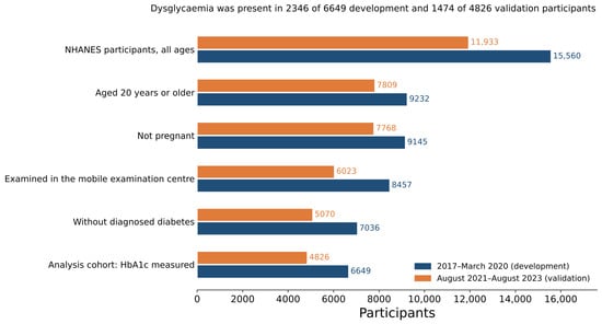
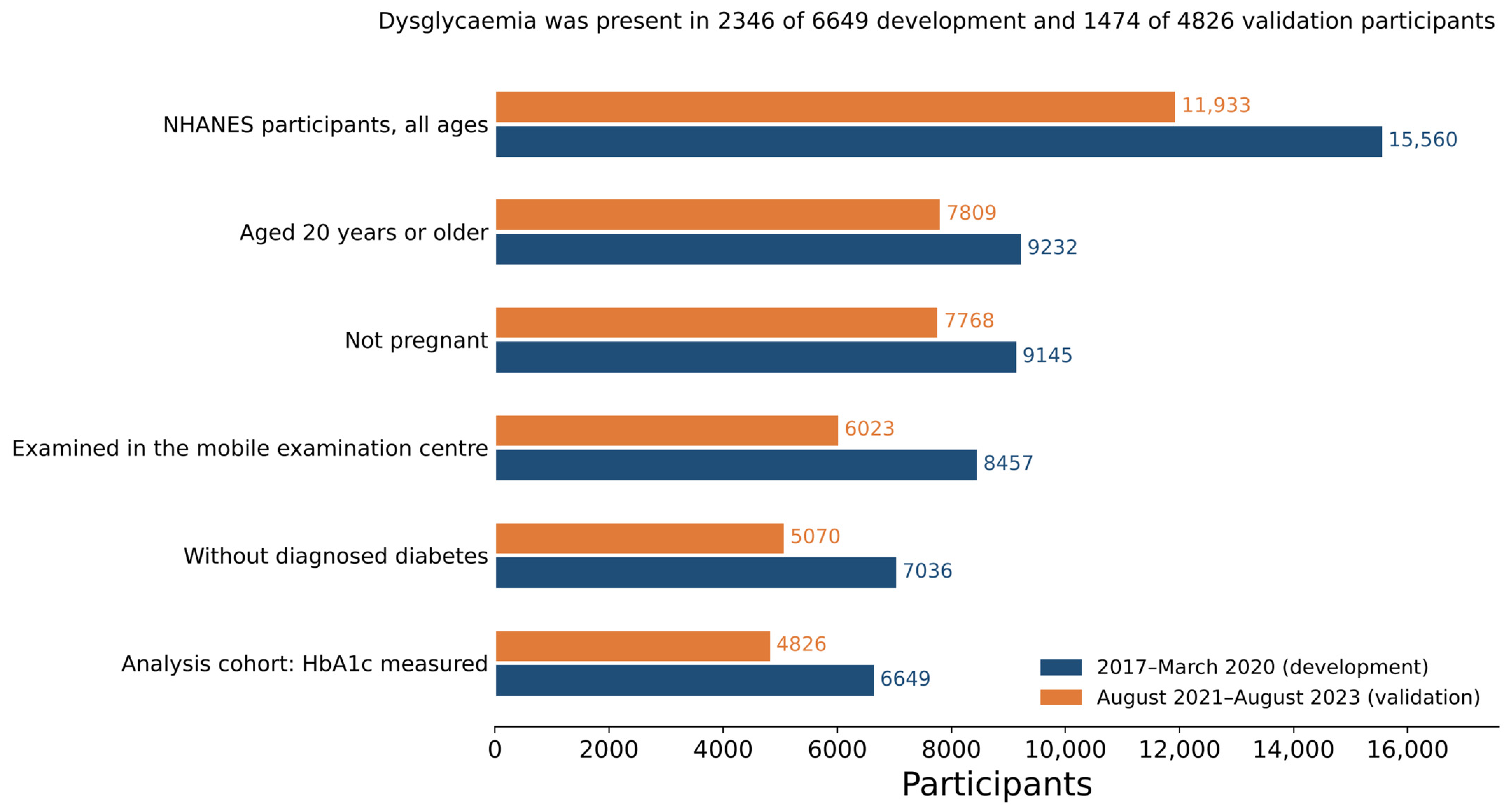
Of the 15,560 participants in the development cycle and 11,933 in the validation cycle, 6649 and 4826 met all criteria and had a measured HbA1c (Figure 1). Diagnosed diabetes excluded 1421 and 953 participants.
Figure 1.
Participant flow. Counts at each eligibility step for the 2017–March 2020 development cycle and the August 2021–August 2023 validation cycle.
Dysglycaemia was present in 2346 of 6649 (35.3% unweighted) development-cycle and 1474 of 4826 (30.5%) validation-cycle participants; applying survey weights, the prevalence values in United States adults without diagnosed diabetes were 27.1% and 26.7%. Undiagnosed diabetes accounted for 237 and 128 of these, the remainder being prediabetes.
Participants with dysglycaemia were on average twelve years older (weighted mean: 56.0 versus 43.5 years), more obese (body mass index: 31.5 versus 28.5 kg/m2; waist: 105.5 versus 96.8 cm), more hypertensive (systolic pressure: 126.8 versus 119.1 mmHg; 41.5% versus 22.8% said they had high blood pressure), more dyslipidaemic (median triglycerides: 128.0 versus 102.0 mg/dL; HDL cholesterol: 51.6 versus 55.8 mg/dL), more inflamed (median high-sensitivity C-reactive protein: 2.6 versus 1.4 mg/L), and had lower renal function (eGFR: 90.2 versus 100.1 mL/min/1.73 m2); all of these differences were significant at p < 0.001, whereas the proportion of men and of current smokers did not differ in the development cycle. Full weighted characteristics for both cycles are given in Table 1.
Table 1.
Weighted participant characteristics by dysglycaemia status; both cycles.
3.2. Model Performance
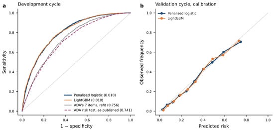
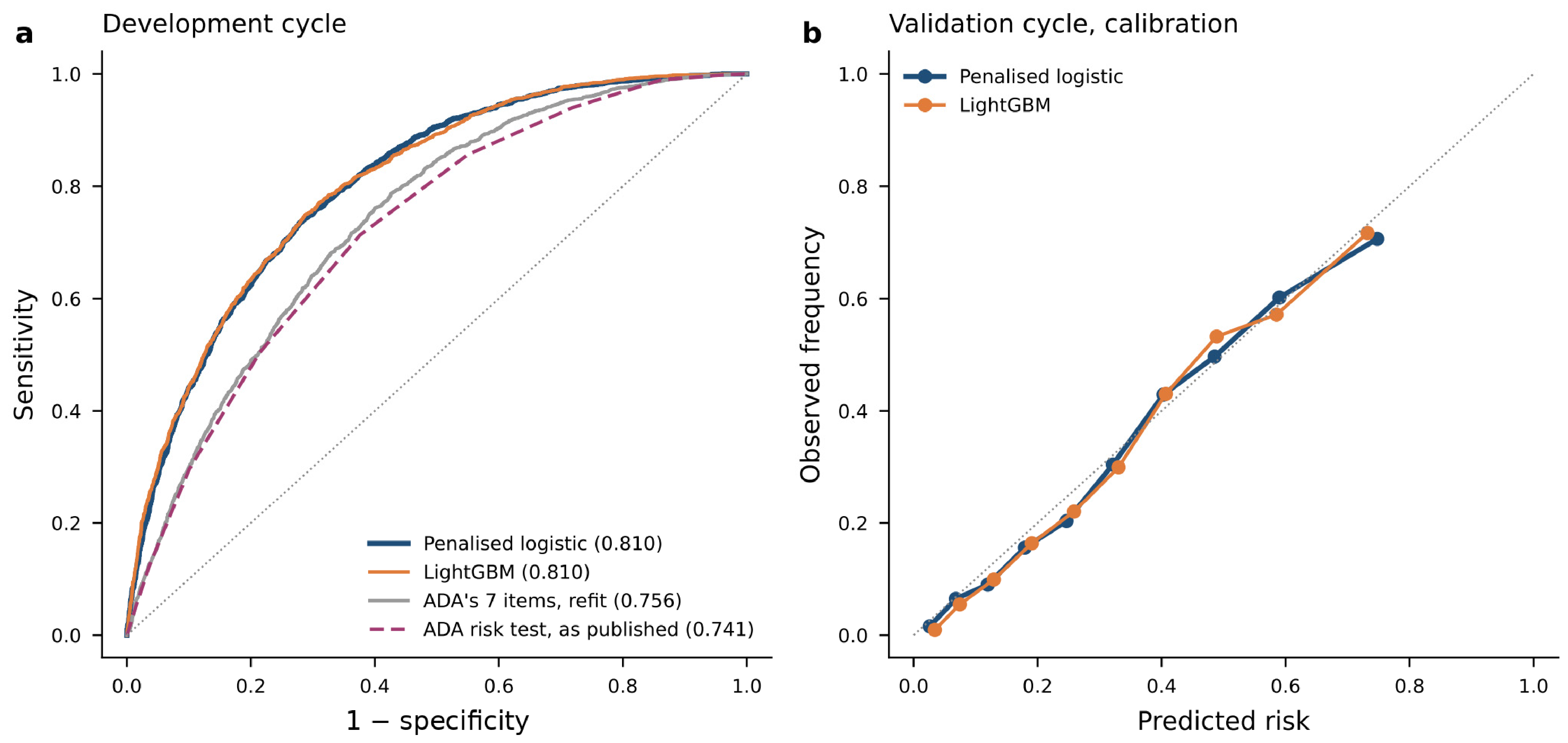
The penalised logistic regression achieved a weighted AUROC of 0.810 (95% CI 0.788 to 0.830) in internal nested cross-validation and 0.818 (0.799 to 0.835) in the frozen validation cycles (Figure 2a). Predicted risks matched observed frequencies closely in both cycles, with a calibration slope of 1.04 (0.94 to 1.14) in development and 1.08 (1.00 to 1.16) in validation and slight overprediction in the upper deciles (Figure 2b); externally, the observed-to-expected ratio was 0.957 (0.895 to 1.017), so a small overprediction is present overall and not only at the top of the range. Bootstrap optimism was small, and the optimism-corrected estimate of 0.804 is close to the cross-validated one. Confidence intervals for all performance measures are given in Table 2.
Figure 2.
Discrimination and calibration. (a) Receiver operating characteristic curves in the development cycle for the penalised logistic regression, LightGBM, the seven ADA items with weights refit in this population, and the published ADA risk test; weighted area under the curve in parentheses. (b) Calibration by decile of predicted risk in the validation cycle. All estimates use mobile-examination-centre survey weights.
Table 2.
Discrimination, calibration, and overall accuracy of the three models, internal and external, with 95% confidence intervals.
Neither gradient-boosting model improved on the regression. The paired difference in the development cycle was −0.0004 (−0.0074 to +0.0065; p = 0.92) for LightGBM and −0.0020 (−0.0096 to +0.0058; p = 0.64) for XGBoost, and +0.0039 (−0.0019 to +0.0090; p = 0.19) and +0.0021 (−0.0034 to +0.0067; p = 0.46) in the validation cycle. Both gradient-boosting models showed more optimism and slightly steeper validation calibration slopes than the regression (Table 2). The penalised regression was therefore retained as the primary model. Its coefficients, knot locations, and intercept are given in full in Table S1 with a reference implementation, and a single pooled equation reproduces the multiply imputed model to within 0.007 in predicted probability; so, the model can be applied as an equation without repeating the imputation procedure.
3.3. Comparison with the ADA Risk Test
The ADA risk test achieved a weighted AUROC of 0.741 (0.721 to 0.758) across all 6649 development-cycle participants. The penalised regression exceeded it by 0.0694 (0.0493 to 0.0906; p < 0.001) on the same participants (Table 3A). In the 5763 participants in whom every questionnaire item was observed, so that no rule for unobserved items was needed, the questionnaire reached 0.730 and the difference was 0.0720 (0.0483 to 0.0968; p < 0.001) (Table S7).
Table 3.
(A) Paired comparisons between models and against the ADA risk test. (B) Decomposition of the advantage over the published ADA risk test.
Decomposing that advantage (Table 3B), refitting the same seven ADA items in this population raised discrimination to 0.756 (0.737 to 0.774), a paired gain of 0.0150 (0.0061 to 0.0245; p < 0.001); moving to the full model raised it further to 0.810, a paired difference of 0.0544 (0.0384 to 0.0711; p < 0.001). The two models in the second step are not nested: the full model adds the 44 predictors that are not ADA items and at the same time omits three self-reported items the questionnaire collects; so, 0.0544 is the net effect of that change in predictor set and not the value of the added measurements alone. Because all three steps are evaluated on the same participants, the two differences sum to the total advantage of 0.0694. About one-fifth of the advantage is therefore attributable to refitting the questionnaire’s own items to a contemporary population, and the remaining four-fifths to the net change from those items to the full set of routine measurements.
3.4. Clinical Utility
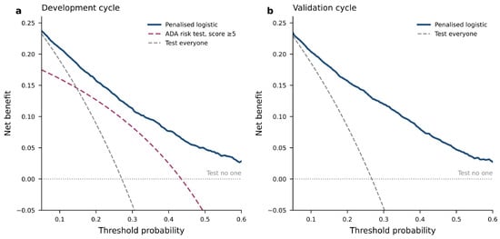
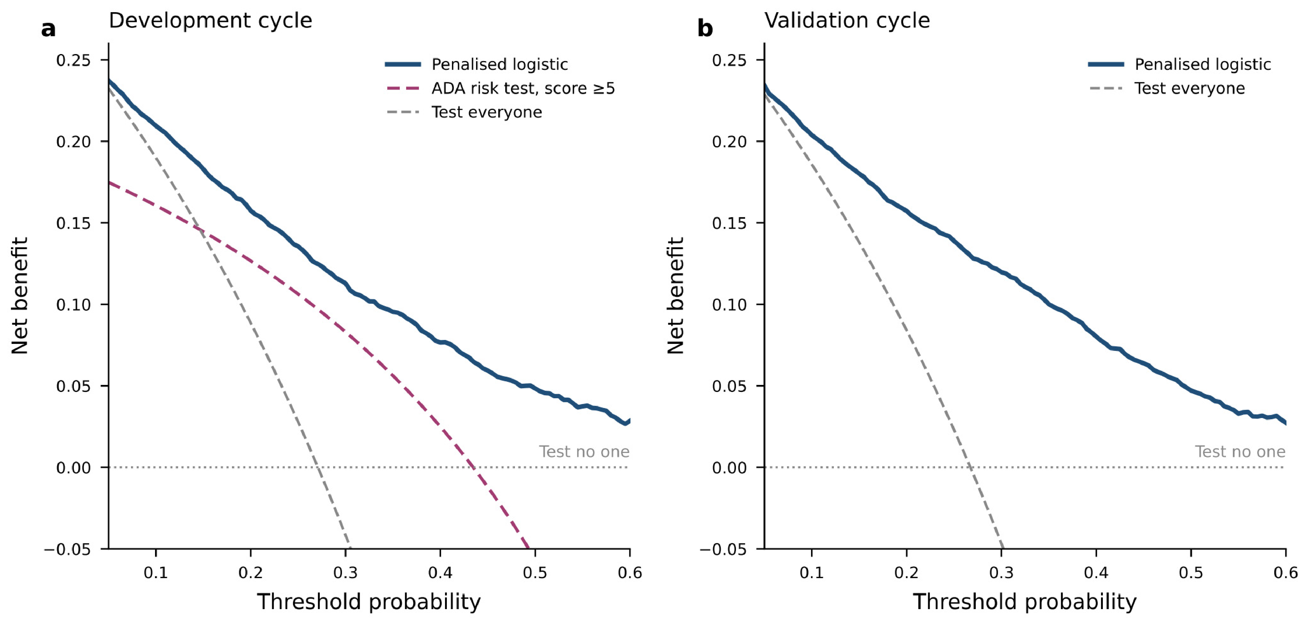
Decision-curve analysis in the development cycle used the out-of-fold predictions. Across threshold probabilities ranging from 0.05 to 0.60, the model had a higher net benefit than the questionnaire applied at its action threshold of 5, by between 0.0268 and 0.2071 per participant, the smallest margin falling at a threshold of 0.265; the bootstrap confidence interval for the difference excluded zero at every tabulated threshold (Table S6, Figure 3a). The model also exceeded testing everyone and testing no one throughout that range. In the validation cycle, where the questionnaire cannot be computed, the model remained superior to both defaults throughout (Figure 3b).
Figure 3.
Decision curves. (a) Development cycle, comparing the penalised logistic regression with the published ADA risk test applied at its own action threshold of 5, with testing everyone and with testing no one. The questionnaire enters as a fixed binary rule because its score is not calibrated to a probability; so, its net benefit varies with the threshold only through the weighting of false positives. Development-cycle curves use out-of-fold predictions; confidence intervals for the net-benefit differences at tabulated thresholds are given in Table S6. (b) Validation cycle, where the questionnaire is not computable because two of its items were not collected. All estimates use mobile-examination-centre survey weights.
Table 4 translates this into the triage decision. Testing everyone requires 3.69 HbA1c measurements per case of dysglycaemia found. The ADA risk test at its action threshold of 5 sends 43.2% of the population for testing, finds 69.3% of cases, and requires 2.30 tests per case. At the same specificity, the model sends 46.0% for testing and finds 79.9% of cases, 10.6 percentage points more (95% CI 5.9 to 15.0; p < 0.001), with a negative predictive value of 89.9% against the ADA test’s 85.4%. At the pre-specified threshold of 0.30, the model sends 39.6% for testing and finds 73.0% of cases: 3.6 percentage points fewer tests than the questionnaire (95% CI 1.7 to 5.4), for 3.8 percentage points more cases found (−0.4 to 8.1); the reduction in tests is statistically distinguishable from zero, whereas the interval for the gain in cases found at this threshold includes zero. As a survey-based projection rather than an observed implementation outcome, in a population of 100,000 adults who already have a panel on file, this corresponds to about 1000 additional cases detected on about 3600 fewer assays. These operating characteristics were transported to the validation cycle almost unchanged: at the same 0.30 threshold, 40.7% were selected for testing, 77.1% of cases were found, and 1.98 tests were required per case.
Table 4.
Operating characteristics and testing burden at candidate thresholds.
3.5. Predictor Contributions
The importance ranking was highly stable across imputations and reasonably stable across cross-validation folds, but the two importance methods agreed only moderately with each other (median Kendall’s tau 0.91, 0.77, and 0.59); so, the ranking is indicative rather than definitive.
Under the gradient-boosting explainer, age contributed more than twice as much as any other predictor, followed by race and Hispanic origin; the next eight, in order, were mean corpuscular volume, total bilirubin, alcohol intake, the AST/ALT ratio, high-sensitivity C-reactive protein, waist-to-hip ratio, gamma-glutamyl transferase, and waist-to-height ratio. Age and race also ranked first and second under the regression’s linear-explainer decomposition, but the two methods organize the remainder differently. High-sensitivity C-reactive protein ranks third under the regression and seventh under the gradient-boosting model; systolic pressure fifth and fourteenth; and alcohol intake fourteenth and fifth. Waist circumference ranks thirtieth under both. Body mass index falls outside the top ten under the gradient-boosting explainer (rank 23) but inside it under the regression (rank 10); so, no claim that anthropometry is displaced by the ratio measures survives both methods. Both rankings are given in Table S4.
3.6. Subgroup Performance
Discrimination varied across subgroups (Table S5). It was similar in men and women: 0.805 (0.782 to 0.827) and 0.816 (0.797 to 0.836) in the development cycle; 0.807 (0.780 to 0.830) and 0.829 (0.809 to 0.847) in validation. It fell steeply with age, from 0.838 (0.806 to 0.864) in participants aged 20 to 39 years to 0.759 (0.725 to 0.790) at 40 to 59 years and 0.712 (0.679 to 0.743) at 60 years or older, with the same ordering in the validation cycle. This is expected where age is the dominant predictor, because discrimination within an age stratum cannot draw on it. Across race and Hispanic origin, development-cycle estimates ranged from 0.724 (0.638 to 0.809) in the other or multiracial group, the smallest group and the one with the widest interval, to 0.834 (0.797 to 0.867) in other Hispanic participants; among the five groups with at least 500 participants, the spread was 0.790 to 0.834. In the validation cycle, the range was from 0.727 (0.675 to 0.776) in non-Hispanic Black participants to 0.852 (0.791 to 0.902) in non-Hispanic Asian participants, with non-Hispanic White participants at 0.832 (0.810 to 0.852). Several of these groups are small and their intervals overlap, so the ordering within them should not be over-read; the gap between the lowest and the highest estimate, however, is wider than the overall confidence interval.
3.7. Sensitivity Analyses
Discrimination of the primary model was stable across the pre-specified variations, ranging from 0.761 when the cohort was restricted to age 35 years or older, as expected when the strongest predictor’s range is truncated, to 0.839 when the outcome was narrowed to an HbA1c threshold of 6.0%. Broadening the outcome to HbA1c 5.7% or higher or fasting plasma glucose 100 mg/dL or higher in the fasting subpopulation gave 0.779; this outcome is met by 65.0% of that subpopulation, against 35.3% for HbA1c alone in the full cohort, so it is a substantially more inclusive label. Excluding participants with chronic kidney disease, fitting with survey weights, and restricting this to complete cases all left discrimination between 0.806 and 0.813 (Table S3).
The conclusion that gradient boosting does not improve on regression also held: in eight of the ten pre-specified analyses, the confidence interval for the difference included zero (Table S3). The two exceptions were the analyses with the fewest events: the HbA1c 6.0% threshold, where LightGBM exceeded the regression by +0.0124 (+0.0004 to +0.0257; p = 0.038), and the undiagnosed-diabetes secondary outcome, +0.0291 (+0.0069 to +0.0523; p = 0.010). Neither would be declared significant at the Bonferroni-adjusted threshold of 0.005 for ten comparisons.
Three analyses bear directly on the modelling decisions. Adding physical activity to the main model changed discrimination by −0.0002 (−0.0007 to +0.0001; p = 0.23) in a paired comparison on the same participants; so, excluding it on instrument grounds had no measurable cost. Re-including the excluded self-report of high blood glucose raised discrimination to 0.820, a paired gain of +0.0095 (+0.0035 to +0.0156; p < 0.001), which quantifies what the model gives up by refusing that leakage. Adding the non-fasting serum glucose that is part of the metabolic panel gave 0.834, a paired gain of +0.0240 (+0.0184 to +0.0295; p < 0.001). A model restricted to the ten strongest predictors reached 0.800; so, most of the discrimination survives a considerably lighter data requirement (Table S3). Forming the cross-validation folds at the level of the primary sampling unit rather than the participant gave a weighted AUROC of 0.812 for the regression, against 0.810 with participant-level folds.
4. Discussion
In a nationally representative sample of adults without diagnosed diabetes, variables already present in a routine clinical encounter identified prevalent dysglycaemia with an AUROC of 0.81, reproduced at 0.82 in a later, independently collected survey cycle held back until the model was final. In the development cycle, the only cycle in which the questionnaire could be scored, this exceeded the published ADA risk test by 0.069. At the questionnaire’s own operating point, the model found more than ten percentage points more cases; at a threshold of 0.30, it tested fewer people, with a gain in cases found whose confidence interval included zero. Gradient boosting did not improve on a penalised regression, reproducing on these data what a systematic review of clinical prediction models had already concluded [14]; the contribution here is that the comparison was made under a matched tuning protocol on a clinical question where the questionnaire it replaces is in active use, and that the deployable result is therefore an equation.
Two subgroup findings temper the clinical message. Discrimination was substantially lower in adults aged 60 years or older, who carry most of the dysglycaemia in this population. So, the model ranks risk the worst in the group where most cases are; and in the validation cycle, its discrimination performance was worse in non-Hispanic Black participants (0.727) than in non-Hispanic White (0.832) or non-Hispanic Asian participants (0.852). A single threshold applied across the whole population would therefore not allocate testing equally, and both patterns need examining before any implementation.
The decomposition is, we think, the most useful finding for anyone maintaining a risk score. About one-fifth of the model’s advantage was attributable to refitting the ADA items in a contemporary population, and the remaining four-fifths to the net change from those seven items to the full set of routine measurements. Recalibrating an existing instrument is therefore worth doing; but, in this population, it left the refitted seven-item score at approximately 0.76, and the step to the measured predictor set accounted for most of the remaining gain. Two qualifications apply. The second step changes the predictor set rather than adding to it, so the value of the measurements alone, and the incremental value of the omitted questionnaire items when added to the full model, were not estimated. And the comparison establishes that the measured predictors outperform the questionnaire where both are available; it does not establish that the questionnaire would add nothing to the measured predictors, which was not tested.
Three design choices deserve comments. The composite outcome of HbA1c 5.7% or higher was chosen because it defines the population in whom a clinical action follows a positive screen, namely confirmatory testing, lifestyle referral, or, in some cases, pharmacotherapy, and because it supports a stable estimation, whereas undiagnosed diabetes alone would have given five events per predictor. Physical activity was held to two different standards, deliberately: a predictor carried into external validation must behave comparably in both survey releases, which the activity instrument did not, whereas the comparator is scored in the development cycle only and never has to transport, and scoring the questionnaire without an item it specifies would have handicapped it. Glucose was excluded from the predictor set because it is itself a diagnostic glycaemic measurement: fasting glucose and HbA1c are the tests that define dysglycaemia, and a model that uses one glycaemic test to decide whether to order another answers a narrower question. A non-fasting glucose value is, however, present on most metabolic panels, and a sensitivity analysis quantifies what its exclusion costs: adding it raised discrimination by +0.0240 (+0.0184 to +0.0295). Non-fasting glucose is not a diagnostic criterion for prediabetes [2], so this gain is informational rather than a substitute for the glycaemic test; where fasting glucose has already been measured, this result rather than any model should guide the decision.
The variables that carried the extra signal are not the ones a diabetes risk score would nominate. Age and race were expected. Mean corpuscular volume, total bilirubin, alcohol intake, and the AST/ALT ratio were not. Waist circumference ranked thirtieth under both importance methods, below the waist-to-hip and waist-to-height ratios, while body mass index ranked tenth under the regression explainer and twenty-third under the gradient-boosting one; so, its standing depends on which method is used. We are cautious about interpreting these individually, for three reasons. The two importance methods agreed only moderately with each other. HbA1c is itself sensitive to erythrocyte turnover, so mean corpuscular volume may contribute partly through the measurement rather than through glucose metabolism. And the hepatic markers plausibly reflect the steatotic liver disease that accompanies insulin resistance. What the ranking does establish is that the additional predictive information is distributed across routine haematology and biochemistry rather than concentrated in one overlooked test.
One question the analysis leaves open is which ordering decision the model is for, and the answer determines how its utility should be priced. We intend it for add-on ordering on a specimen already being drawn, or on a panel already in the record: the patient is in the clinic, the complete blood count and metabolic panel exist or are being collected, and the decision is whether to add a glycaemic assay to that order. The resource being allocated is therefore the assay and the reflex-testing workflow rather than a patient encounter, and the testing burden in Table 4 should be read as assays rather than visits. This bounds the claim in both directions. The saving is modest in absolute cost, because an added HbA1c on an existing specimen is among the cheapest decisions in the workflow; what the model buys is detection at the same specificity, 10.6 percentage points more cases than the questionnaire. And where the decision is genuinely expensive, because no specimen has been drawn and no panel exists, the model cannot be computed at all and a questionnaire remains the only available instrument. The retrospective alternative, sweeping existing records to identify never-tested patients who have a panel on file, is a different deliverable measured against current practice rather than against a self-administered score, and we have not evaluated it here.
For the clinician, the model returns a probability, and the threshold at which it prompts a glycaemic test is a policy choice rather than a property of the model. Three settings bracket the reasonable range, using validation-cycle figures. A threshold of 0.20 sends just over half of patients for testing and finds 88% of cases, appropriate where the priority is detection and the marginal cost of an HbA1c is low. A threshold of 0.30 sends 41% and finds 77%, requiring two tests per case detected against 3.7 if everyone is tested. A threshold of 0.40 sends 29% and finds 62%, which suits a constrained laboratory budget but misses two cases in five. What the model does not do at any threshold is exclude dysglycaemia: at 0.30, the negative predictive value is 90%; so, roughly one in ten patients below the threshold still has an HbA1c of 5.7% or above. The output is a reason to test sooner rather than a reason not to test, and a patient whose clinical picture warrants a glycaemic measurement should have one whatever the model returns.
That gradient boosting did not outperform regression is consistent with the broader prediction literature, where a systematic comparison found no performance benefit of machine learning over logistic regression for clinical prediction [14]. Our sensitivity programme adds a detail worth noting: the only two analyses in which gradient boosting showed a nominal advantage were the two with the fewest events, and neither difference survives adjustment for the ten comparisons made. Both involved a narrower, rarer outcome than the primary one, and in that setting performance estimates are less stable. We raise this as an observation rather than a demonstration, since two analyses cannot establish a pattern, but it suggests that where a flexible model does appear to win, the event count deserves inspection before the advantage is believed.
Our results differ from the most comparable prior studies in ways that follow from design. A machine learning analysis of Korean survey data reported areas under the curve values from 0.79 to 0.82 against 0.74 to 0.77 for traditional statistical models, using feature sets of four to seven variables [11]; our comparison produced no such separation. Since the size of an apparent machine learning advantage depends on how carefully the regression comparator is specified [14], the two results are not necessarily in conflict; differences in population, outcome definition, predictor sets, and validation procedure limit any direct comparison, and a difference in how carefully the regression comparator was specified is one possible explanation among several. An NHANES analysis using 114 nutritional markers alongside behavioural and socio-economic variables ranged from 0.749 to 0.757 and was on a par with the ADA risk test on both internal and external validation [12]; that is a lower level than ours reached with more variables, which suggests dietary and behavioural self-report contributes less than routine laboratory measurement. A study restricted to adults aged 20 to 39 years reported 0.69 in men and 0.92 in women against 0.61 and 0.71 for the ADA test [25]; we did not observe such a sex disparity, which, in that study, may reflect the narrow age range and the low number of events.
The closest comparison is a primary-care study that combined the Finnish Diabetes Risk Score with fifteen routine laboratory and clinical variables in a gradient-boosting model and found the questionnaire almost impossible to improve on: 0.835 for the score alone, 0.840 with the routine variables added, and a difference of 0.005 (95% CI −0.012 to 0.022), while the routine variables without the score reached only 0.758 [13]. Read beside ours, this looks like a contradiction, but is not one for two reasons visible in the instruments themselves. The Finnish score contains an item asking whether the patient has ever been found to have elevated blood glucose, which the ADA risk test does not; in a population screened for previously unrecognised dysglycaemia, this item precisely imports the prior glycaemic information our model is required to do without, and the authors of that study name it as a reason for the score’s performance. Second, body mass index and waist circumference sit inside the Finnish score; so, the feature set evaluated without it contained no measure of adiposity at all, whereas ours contains both. The designs also differ: a single centre, one random split with internal hold-out only, and a 46.0% prevalence of an outcome defined from fasting glucose or HbA1c that the authors describe as risk-enriched, against a nationally representative sample with a 27.1% weighted prevalence and validation in a separate later cycle. The two findings are compatible. One explanation consistent with both is that a questionnaire carrying a prior-glucose item already contains much of the information that routine laboratory data would add, whereas one without such an item does not; this is a hypothesis suggested by the two instruments rather than a conclusion either study tested directly, and populations, outcomes, and validation designs also differ.
Several limitations constrain what can be claimed. The design is cross-sectional, so the model estimates prevalent dysglycaemia and says nothing about incidence; it is a triage tool for testing, not a tool for predicting future diabetes. Three things would move this from a validated equation towards a usable one: external validation in a health-system population rather than a survey sample, where the predictor set is recorded as clinical routine rather than as research measurement; subgroup-specific examination of the age and race gradients reported here, with thresholds set accordingly rather than uniformly; and a prospective evaluation of whether acting on the equation changes how many cases are found per test ordered, which no retrospective analysis can establish. The outcome rests on a single HbA1c, which misclassifies relative to repeated testing or an oral glucose tolerance test; no tolerance test was performed in either cycle. The ADA comparator could not be evaluated in the validation cycle because two of its items were not collected, so the head-to-head comparison rests on the development cycle alone, and the physical-activity instrument changed sufficiently between cycles that we could not carry that predictor into validation. Both cycles are United States samples, and transportability to other health systems is untested. Local validation would be required before use elsewhere, and the race and Hispanic origin variable, which ranked second in importance, has no direct equivalent in most other populations; a model intended for another setting would have to be refitted rather than transplanted. The model requires a laboratory panel, so it applies to patients who have had blood drawn for another reason and cannot replace questionnaires in community settings; five of its predictors (income-to-poverty ratio, hip and arm circumference, alcohol intake in grams per day, and high-sensitivity C-reactive protein) are not part of every record, and in settings where they are not collected, the equation would need refitting without them. The cost analysis in Table 4 counts assays, not encounters. Where the specimen drawn for the complete blood count is still available, HbA1c can be added to it; where it is not, a return visit is required, and the time, travel, and clinic costs of that visit are not captured here and would narrow the advantage over a questionnaire completed at the same visit. Finally, the cross-validation folds were formed at the participant level; forming them at the level of the primary sampling unit changed the regression’s AUROC by less than 0.005, so clustering within sampling units did not materially inflate the internal estimate.
Two directions follow. The first is validation in an electronic-health-record cohort, where the intended use case actually occurs and where the number of tests avoided can be counted rather than estimated. The second is an implementation question we cannot answer from survey data: whether presenting a clinician with a risk estimate at the point of the testing decision changes the decision, and whether the change improves detection.
Two practical points follow for anyone implementing the equation. It is defined for a complete predictor set. Where a value is missing, the frozen development-cycle imputation model, which draws on the other predictors and uses no outcome information, can be applied before the equation, exactly as was done for the 31.4% of validation-cycle participants with at least one missing predictor; among the 68.6% with complete data, the AUROC was 0.815 (0.793 to 0.837). The imputation model is deposited with the code. Where that is impractical, the clinician falls back on the questionnaire or on testing. The equation returns a probability and needs no interpretation beyond entering measured values, so no specialist expertise is required of the user, but the choice of threshold is a local decision about testing capacity rather than a property of the model.
5. Conclusions
Among adults without diagnosed diabetes who already have a metabolic panel and a complete blood count on file, routinely available clinical and laboratory data identified prevalent dysglycaemia with an AUROC of 0.81 internally and 0.82 in a later survey cycle. In the development cycle, the only cycle in which the questionnaire could be scored, the model exceeded the published ADA risk test by 0.069; about one-fifth of that advantage was attributable to refitting the questionnaire’s items and the remainder to the net change to routine measurements. Gradient boosting did not improve on a penalised logistic regression; so, the result can be published as a transparent equation, applicable where a metabolic panel and a complete blood count are already on file and the decision is whether to add a glycaemic assay.
Supplementary Materials
The following supporting information can be downloaded at: https://www.mdpi.com/article/10.3390/healthcare14223903/s1: Table S1: Predictors, model terms, fitted coefficients, spline knot locations and intercept of the penalised logistic regression; Table S2: Missing data by predictor and cycle; Table S3: Pre-specified sensitivity analyses S1–S10; Table S4: SHAP importance ranking with stability statistics; Table S5: Discrimination of the penalised logistic regression within subgroups defined by sex, age band and race and Hispanic origin, both cycles; Table S6: Development cycle: differences in net benefit and in operating characteristics between the penalised logistic regression and the ADA risk test applied at its action threshold of 5, with 95% confidence intervals from 2000 Rao–Wu bootstrap replicates resampling primary sampling units within strata; Table S7: Model versus ADA risk test under two treatments of unobserved questionnaire items, and paired sensitivity comparisons of the penalised logistic regression against the main model; Table S8: Imputation diagnostics, development cycle, first of 20 imputations: observed versus imputed distributions for predictors with more than 5% missingness; File S1: Populated TRIPOD+AI checklist.
Author Contributions
Conceptualization, E.Z. and M.Y.; methodology, E.Z.; software, E.Z.; validation, E.Z. and M.Y.; formal analysis, E.Z.; investigation, E.Z.; data curation, E.Z.; writing—original draft preparation, E.Z.; writing—review and editing, E.Z. and M.Y.; visualization, E.Z.; supervision, M.Y. All authors have read and agreed to the published version of the manuscript.
Funding
This research received no external funding.
Institutional Review Board Statement
Not applicable.
Informed Consent Statement
Not applicable.
Data Availability Statement
The NHANES data analysed here are public and available from the Centers for Disease Control and Prevention at https://wwwn.cdc.gov/nchs/nhanes/ (accessed on 10 November 2026). The analysis code, the fitted coefficient table, and a reference implementation of the risk equation are openly available on Zenodo under the MIT licence at https://doi.org/10.5281/zenodo.24054049.
Acknowledgments
The authors thank the NHANES participants and the staff of the National Center for Health Statistics, whose public release of these data made the study possible.
Conflicts of Interest
The authors declare that they have no competing interests.
Abbreviations
The following abbreviations are used in this manuscript:
| ADA | American Diabetes Association |
| AUROC | Area under the receiver operating characteristic curve |
| CI | Confidence interval |
| CKD-EPI | Chronic Kidney Disease Epidemiology Collaboration |
| eGFR | Estimated glomerular filtration rate |
| HbA1c | Glycated haemoglobin |
| NHANES | National Health and Nutrition Examination Survey |
| SHAP | SHapley Additive exPlanations |
| TRIPOD + AI | Transparent Reporting of a multivariable prediction model for Individual Prognosis Or Diagnosis + artificial intelligence extension |
References
- Liu, J.; Yi, S.S.; Russo, R.; Mayer, V.L.; Wen, M.; Li, Y. Trends and disparities in diabetes and prediabetes among adults in the United States, 1999–2018. Public Health 2022, 214, 163–170. [Google Scholar] [CrossRef] [Scilit] [PubMed]
- American Diabetes Association Professional Practice Committee. 2. Diagnosis and classification of diabetes: Standards of Care in Diabetes—2025. Diabetes Care 2025, 48, S27–S49. [Google Scholar] [CrossRef] [Scilit] [PubMed]
- Bang, H.; Edwards, A.M.; Bomback, A.S.; Ballantyne, C.M.; Brillon, D.; Callahan, M.A.; Teutsch, S.M.; Mushlin, A.I.; Kern, L.M. Development and validation of a patient self-assessment score for diabetes risk. Ann. Intern. Med. 2009, 151, 775–783. [Google Scholar] [CrossRef] [Scilit] [PubMed]
- Lindström, J.; Tuomilehto, J. The diabetes risk score: A practical tool to predict type 2 diabetes risk. Diabetes Care 2003, 26, 725–731. [Google Scholar] [CrossRef] [Scilit] [PubMed]
- Heikes, K.E.; Eddy, D.M.; Arondekar, B.; Schlessinger, L. Diabetes Risk Calculator: A simple tool for detecting undiagnosed diabetes and pre-diabetes. Diabetes Care 2008, 31, 1040–1045. [Google Scholar] [CrossRef] [Scilit] [PubMed]
- Griffin, S.J.; Little, P.S.; Hales, C.N.; Kinmonth, A.L.; Wareham, N.J. Diabetes risk score: Towards earlier detection of type 2 diabetes in general practice. Diabetes Metab. Res. Rev. 2000, 16, 164–171. [Google Scholar] [CrossRef] [PubMed]
- Ture, N.; Emecen, A.N.; Unal, B. Validation of the Finnish Diabetes Risk Score and development of a country-specific diabetes prediction model for Turkey. Prim. Health Care Res. Dev. 2025, 26, e18. [Google Scholar] [CrossRef] [Scilit] [PubMed]
- Atayoglu, A.T.; Inanc, N.; Başmisirli, E.; Çapar, A.G. Evaluation of the Finnish Diabetes Risk Score (FINDRISC) for diabetes screening in Kayseri, Turkey. Prim. Care Diabetes 2020, 14, 488–493. [Google Scholar] [CrossRef] [Scilit] [PubMed]
- Kengne, A.P.; Beulens, J.W.; Peelen, L.M.; Moons, K.G.; van der Schouw, Y.T.; Schulze, M.B.; Spijkerman, A.M.; Griffin, S.J.; Grobbee, D.E.; Palla, L.; et al. Non-invasive risk scores for prediction of type 2 diabetes (EPIC-InterAct): A validation of existing models. Lancet Diabetes Endocrinol. 2014, 2, 19–29. [Google Scholar] [CrossRef] [Scilit] [PubMed]
- Yildiz, M.; Yiğitbaş, Ç.; Genç, A.C.; Türkoğlu Genç, F.; Zafer, E.; Muhtaroğlu, A.; Acar, B.; Aslan, S.; Kuloğlu, E.; İşsever, K. Can the Finnish Diabetes Risk Score (FINDRISC) be used to predict liver fibrosis risk instead of the fibrosis-4 index (FIB-4)? Fam. Pract. 2026, 43, cmag008. [Google Scholar] [CrossRef] [Scilit] [PubMed]
- Choi, S.G.; Oh, M.; Park, D.H.; Lee, B.; Lee, Y.H.; Jee, S.H.; Jeon, J.Y. Comparisons of the prediction models for undiagnosed diabetes between machine learning versus traditional statistical methods. Sci. Rep. 2023, 13, 13101. [Google Scholar] [CrossRef] [Scilit] [PubMed]
- De Silva, K.; Lim, S.; Mousa, A.; Teede, H.; Forbes, A.; Demmer, R.T.; Jönsson, D.; Enticott, J. Nutritional markers of undiagnosed type 2 diabetes in adults: Findings of a machine learning analysis with external validation and benchmarking. PLoS ONE 2021, 16, e0250832. [Google Scholar] [CrossRef] [Scilit] [PubMed]
- Türkoğlu Genç, F.; Yildiz, M. The Finnish Diabetes Risk Score (FINDRISC) combined with explainable machine learning for detection of previously unrecognized dysglycemia in primary care: A CatBoost-based approach. Healthcare 2026, 14, 3214. [Google Scholar] [CrossRef] [Scilit] [PubMed]
- Christodoulou, E.; Ma, J.; Collins, G.S.; Steyerberg, E.W.; Verbakel, J.Y.; Van Calster, B. A systematic review shows no performance benefit of machine learning over logistic regression for clinical prediction models. J. Clin. Epidemiol. 2019, 110, 12–22. [Google Scholar] [CrossRef] [Scilit] [PubMed]
- Collins, G.S.; Moons, K.G.M.; Dhiman, P.; Riley, R.D.; Beam, A.L.; Van Calster, B.; Ghassemi, M.; Liu, X.; Reitsma, J.B.; van Smeden, M.; et al. TRIPOD+AI statement: Updated guidance for reporting clinical prediction models that use regression or machine learning methods. BMJ 2024, 385, e078378. [Google Scholar] [CrossRef] [Scilit] [PubMed]
- Akinbami, L.J.; Chen, T.C.; Davy, O.; Ogden, C.L.; Fink, S.; Clark, J.; Riddles, M.K.; Mohadjer, L.K. National Health and Nutrition Examination Survey, 2017–March 2020 Prepandemic File: Sample design, estimation, and analytic guidelines. Vital Health Stat. 2022, 190, 1–36. [Google Scholar] [CrossRef] [Scilit]
- Riley, R.D.; Ensor, J.; Snell, K.I.E.; Harrell, F.E.; Martin, G.P.; Reitsma, J.B.; Moons, K.G.M.; Collins, G.; van Smeden, M. Calculating the sample size required for developing a clinical prediction model. BMJ 2020, 368, m441. [Google Scholar] [CrossRef] [Scilit] [PubMed]
- White, I.R.; Royston, P.; Wood, A.M. Multiple imputation using chained equations: Issues and guidance for practice. Stat. Med. 2011, 30, 377–399. [Google Scholar] [CrossRef] [Scilit] [PubMed]
- Sisk, R.; Sperrin, M.; Peek, N.; van Smeden, M.; Martin, G.P. Imputation and missing indicators for handling missing data in the development and deployment of clinical prediction models: A simulation study. Stat. Methods Med. Res. 2023, 32, 1461–1477. [Google Scholar] [CrossRef] [Scilit] [PubMed]
- Hoogland, J.; van Barreveld, M.; Debray, T.P.A.; Reitsma, J.B.; Verstraelen, T.E.; Dijkgraaf, M.G.W.; Zwinderman, A.H. Handling missing predictor values when validating and applying a prediction model to new patients. Stat. Med. 2020, 39, 3591–3607. [Google Scholar] [CrossRef] [Scilit] [PubMed]
- Rao, J.N.K.; Wu, C.F.J. Resampling inference with complex survey data. J. Am. Stat. Assoc. 1988, 83, 231–241. [Google Scholar] [CrossRef]
- Van Calster, B.; McLernon, D.J.; van Smeden, M.; Wynants, L.; Steyerberg, E.W. Calibration: The Achilles heel of predictive analytics. BMC Med. 2019, 17, 230. [Google Scholar] [CrossRef] [Scilit] [PubMed]
- Vickers, A.J.; Elkin, E.B. Decision curve analysis: A novel method for evaluating prediction models. Med. Decis. Mak. 2006, 26, 565–574. [Google Scholar] [CrossRef] [Scilit] [PubMed]
- Lundberg, S.M.; Erion, G.; Chen, H.; DeGrave, A.; Prutkin, J.M.; Nair, B.; Katz, R.; Himmelfarb, J.; Bansal, N.; Lee, S.I. From local explanations to global understanding with explainable AI for trees. Nat. Mach. Intell. 2020, 2, 56–67. [Google Scholar] [CrossRef] [Scilit] [PubMed]
- Srugo, S.A.; de Groh, M.; Jiang, Y.; Morrison, H.I.; Villeneuve, P.J. Evaluating the utility of self-reported questionnaire data to screen for dysglycemia in young adults: Findings from the US National Health and Nutrition Examination Survey. Prev. Med. 2019, 120, 50–59. [Google Scholar] [CrossRef] [Scilit] [PubMed]

Disclaimer/Publisher’s Note: The statements, opinions and data contained in all publications are solely those of the individual author(s) and contributor(s) and not of MDPI and/or the editor(s). MDPI and/or the editor(s) disclaim responsibility for any injury to people or property resulting from any ideas, methods, instructions or products referred to in the content. |
© 2026 by the authors. Licensee MDPI, Basel, Switzerland. This article is an open access article distributed under the terms and conditions of the Creative Commons Attribution (CC BY) license.