Analysis and Computation of Solutions for a Class of Nonlinear SBVPs Arising in Epitaxial Growth

Abstract

In this work, the existence and nonexistence of stationary radial solutions to the elliptic partial differential equation arising in the molecular beam epitaxy are studied. Since we are interested in radial solutions, we focus on the fourth-order singular ordinary differential equation. It is non-self adjoint, it does not have exact solutions, and it admits multiple solutions. Here, $\lambda \in \mathbb{R}$ measures the intensity of the flux and G is stationary flux. The solution depends on the size of the parameter $\lambda$. We use a monotone iterative technique and integral equations along with upper and lower solutions to prove that solutions exist. We establish the qualitative properties of the solutions and provide bounds for the values of the parameter $\lambda$, which help us to separate existence from nonexistence. These results complement some existing results in the literature. To verify the analytical results, we also propose a new computational iterative technique and use it to verify the bounds on $\lambda$ and the dependence of solutions for these computed bounds on $\lambda$.

1. Introduction

Epitaxy means the growth of a single thin film on top of a crystalline substrate. It is crucial for semiconductor thin film technology, hard and soft coatings, protective coatings, optical coatings, etc. The epitaxial growth technique is used to produce the growth of semiconductor films and multilayer structures under high vacuum conditions [1]. The major advantages of epitaxial growth are reducing the growth time, better structural and superior electrical properties, eliminating waste caused during growth, wafering cost, cutting, polishing, etc. Several types of epitaxial growth techniques, such as hybrid vapor phase epitaxy [2], chemical beam epitaxy [3], and molecular beam epitaxy (MBE), have been used for the growth of compound semiconductors and other materials. In this work, we strictly focus on MBE, and we restrict our attention to the differential equation model, which was proposed by Escudero et al. [4,5,6,7]. The mathematical description of epitaxial growth is carried out by means of a function $\sigma$ defined as

$$\begin{array}{c}\hfill \sigma :\Omega \subset {\mathbb{R}}^2\times {\mathbb{R}}^{+}\to \mathbb{R},\end{array}$$

which describes the height of the growing interface in the spatial point $x\in \Omega \subset {\mathbb{R}}^2$ at time $t\in {\mathbb{R}}^{+}$. The authors in [4,5,6,7] show that the function $\sigma$ obeys the fourth-order partial differential equation

$${\partial }_t\sigma +{\Delta }^2\sigma =\det \left(D^2\sigma \right)+\lambda \eta (x,t),x\in \Omega \subset {\mathbb{R}}^2,$$

(1)

where $\eta (x,t)$ models the incoming mass entering the system through epitaxial deposition, $\lambda$ measures the intensity of this flux, and the determinant of Hessian matrix is

$$\det \left(D^2\sigma \right)={\displaystyle \frac{{\partial }^2\sigma }{\partial x_1^2}}·{\displaystyle \frac{{\partial }^2\sigma }{\partial x_2^2}}-{\left({\displaystyle \frac{{\partial }^2\sigma }{\partial x_1\partial x_2}}\right)}^2.$$

(2)

The stationary counterpart of the partial differential Equation (1) subject to the homogeneous Dirichlet boundary condition (4) and homogeneous Navier boundary condition (5) is defined as (see [6])

$$\begin{array}{c}{\Delta }^2\sigma =\det \left(D^2\sigma \right)+\lambda G\left(x\right),x\in \Omega \subset {\mathbb{R}}^2,\hfill \end{array}$$

(3)

$$\begin{array}{c}{\displaystyle \sigma =0,\frac{\partial \sigma }{\partial n}=0\mathrm{on}\partial \Omega ,}\hfill \end{array}$$

(4)

$$\begin{array}{c}{\displaystyle \sigma =0,\Delta \sigma =0\mathrm{on}\partial \Omega ,}\hfill \end{array}$$

(5)

where $\eta (x,t)\equiv G\left(x\right)$ is a stationary flux, and n is the unit out drawn normal to $\partial \Omega$.

Using the transformation $r=\left|x\right|$ and $\sigma \left(x\right)=\varphi \left(\right|x\left|\right)$, as a result of symmetry, the above set of equations are transformed into the following set of equations:

$$\begin{array}{ccc}& & \frac{1}{r}{\left\{r{\left[\frac{1}{r}{\left(r{\varphi }^{\prime }\right)}^{\prime }\right]}^{\prime }\right\}}^{\prime }=\frac{1}{r}{\varphi }^{\prime }{\varphi }^{″}+\lambda G\left(r\right),\hfill \end{array}$$

(6)

$$\begin{array}{ccc}& & {\displaystyle {\varphi }^{\prime }\left(0\right)=0,\varphi \left(1\right)=0,{\varphi }^{\prime }\left(1\right)=0,\underset{r\to 0}{lim}r\varphi ‴\left(r\right)=0,}\hfill \end{array}$$

(7)

$$\begin{array}{ccc}& & {\displaystyle {\varphi }^{\prime }\left(0\right)=0,\varphi \left(1\right)=0,{\varphi }^{\prime }\left(1\right)+{\varphi }^{″}\left(1\right)=0,\underset{r\to 0}{lim}r{\varphi }^{‴}\left(r\right)=0,}\hfill \end{array}$$

(8)

where ${\displaystyle \prime =\frac{d}{dr}}$.

In this paper, we also impose the following boundary conditions which complements the work in [6]:

$$\begin{array}{c}\hfill {\displaystyle {\varphi }^{\prime }\left(0\right)=0,\varphi \left(1\right)=0,{\varphi }^{″}\left(1\right)=0,\underset{r\to 0}{lim}r{\varphi }^{‴}\left(r\right)=0.}\end{array}$$

(9)

For simplicity, we take $G\left(r\right)=1$, which physically means that the new material is being deposited uniformly on the unit disc.

Now, using ${\displaystyle \underset{r\to 0}{lim}r{\varphi }^{‴}\left(r\right)=0}$, $w=r{\varphi }^{\prime }$ and integrating parts from Equation (6), we have

$$\begin{array}{ccccc}\hfill & \hfill & & \hfill & \hfill r^2{w}^{″}-r{w}^{\prime }=\frac{1}{2}{w}^2+\frac{1}{2}\lambda r^4.\end{array}$$

(10)

Using the transformation ${\displaystyle t=\frac{r^2}{2}}$ and $u\left(t\right)=w\left(r\right)$, it is possible to reduce Equation (10) into the following equation:

$$u^{″}=\frac{u^2}{8t^2}+\frac{\lambda }{2},\mathrm{for}t\in \left(0,\frac{1}{2}\right].$$

(11)

Corresponding to (11), we define the following three boundary value problems:

$$\begin{array}{ccc}& & \mathrm{Problem}1:\left\{\begin{array}{c}{\displaystyle u^{″}=\frac{u^2}{8t^2}+\frac{\lambda }{2},\mathrm{for}t\in \left(0,\frac{1}{2}\right]}\hfill \\ {\displaystyle \underset{t\to 0^{+}}{lim}\sqrt{t}{u}^{\prime }\left(t\right)=0,u\left(\frac{1}{2}\right)=0,}\hfill \end{array}\right.\hfill \end{array}$$

(12)

$$\begin{array}{ccc}& & \mathrm{Problem}2:\left\{\begin{array}{c}{\displaystyle u^{″}=\frac{u^2}{8t^2}+\frac{\lambda }{2},\mathrm{for}t\in \left(0,\frac{1}{2}\right]}\hfill \\ {\displaystyle \underset{t\to 0^{+}}{lim}\sqrt{t}{u}^{\prime }\left(t\right)=0,u^{\prime }\left(\frac{1}{2}\right)=0,}\hfill \end{array}\right.\hfill \end{array}$$

(13)

$$\begin{array}{ccc}& & \mathrm{Problem}3:\left\{\begin{array}{c}{\displaystyle u^{″}=\frac{u^2}{8t^2}+\frac{\lambda }{2},\mathrm{for}t\in \left(0,\frac{1}{2}\right]}\hfill \\ {\displaystyle \underset{t\to 0^{+}}{lim}\sqrt{t}{u}^{\prime }\left(t\right)=0,u\left(\frac{1}{2}\right)=u^{\prime }\left(\frac{1}{2}\right).}\hfill \end{array}\right.\hfill \end{array}$$

(14)

The BVPs (12), (13) and (14) can be equivalently described as the following integral equations (IE):

• IE corresponding to Problem 1:

  $$u\left(t\right)=-\left[\left(\frac{1}{2}-t\right){\int }_0^t\frac{u{\left(s\right)}^2}{4s}ds+t{\int }_t^{\frac{1}{2}}\frac{u{\left(s\right)}^2}{4s^2}\left(\frac{1}{2}-s\right)ds+\frac{\lambda }{4}t\left(\frac{1}{2}-t\right)\right],$$

  (15)
• IE corresponding to Problem 2:

  $$u\left(t\right)=-\left[{\int }_0^t\frac{u{\left(s\right)}^2}{8s}ds+t{\int }_t^{\frac{1}{2}}\frac{u{\left(s\right)}^2}{8s^2}ds+\frac{\lambda }{4}t\left(1-t\right)\right],$$

  (16)
• IE corresponding to Problem 3:

  $$u\left(t\right)=-\left[\left(t+\frac{1}{2}\right){\int }_0^t\frac{u{\left(s\right)}^2}{4s}ds+t{\int }_t^{\frac{1}{2}}\frac{u{\left(s\right)}^2}{4s^2}\left(s+\frac{1}{2}\right)ds+\frac{\lambda }{4}t\left(\frac{3}{2}-t\right)\right].$$

  (17)

We assume that $u\in C_{loc}^2\left(\left(0,\frac{1}{2}\right];\mathbb{R}\right)$, where $C_{loc}^2\left(\left(0,\frac{1}{2}\right];\mathbb{R}\right)$ is defined as

$$\left\{u:\left(0,\frac{1}{2}\right]\to \mathbb{R}|u\in C^2\left([a,b],\mathbb{R}\right)\mathrm{for}\mathrm{everycompact}\mathrm{set}[a,b]\subset \left(0,\frac{1}{2}\right]\right\}.$$

In [6], Escudero et al. proved the existence and nonexistence of solutions of Problems 1 and 3 using upper and lower solution techniques. Corresponding to Problems 1 and 3, they have also provided the rigorous bounds of the values of the parameter $\lambda$, which helps us to separate existence from nonexistence. In [8], Verma et al. provide numerical illustrations via VIM to verify the results of Escudero et al. [6]. To verify their numerical results, they provided other iterative schemes based on homotopy [9] and the Adomian decomposition method [10].

Equation (13) has not been investigated theoretically in the existing literature to the best of our knowledge. Moreover, many investigations are still pending relating to BVPs (12), (13), and (14). Here, we focus on both theoretical and numerical work. We derive the sign of the solution and prove its existence in continuous space. We also compute the bounds of the parameter $\lambda$. The results of this paper complements existing theoretical results. We also provide an iterative scheme based on Green’s function to compute the bounds and solutions to demonstrate the existence and nonexistence, which is dependent on $\lambda$.

To prove the existence of the solutions, we use the monotone iterative technique [11,12,13,14,15,16,17]. Recently, many researchers applied this technique on the initial value problem (IVP) for the nonlinear noninstantaneous impulsive differential equation (NIDE) [18], p-Laplacian boundary value problems with the right-handed Riemann–Liouville fractional derivative [19], etc. to prove the existence of the solution. Here, we also present numerical results to verify the theoretical results. To develop the iterative scheme based on Green’s function, we consider Equations (12)–(14). Recently, many authors have used numerical approximate methods like the VIM [8], the Adomian decomposition method (ADM), the homotopy perturbation method (HPM) etc. to find approximate solutions for different models involving differential equations [20,21], integral equations [22,23,24], fractional differential equations [25,26], the Stefan problem [27,28,29,30], system of integral equations [31], etc. Thereafter, Waleed Al Hayani [32] and Singh et al. [33] applied ADM with Green’s function to compute the approximate solution. Recently, Noeiaghdam et al. [34] proposed a technique based on ADM for solving Volterra integral equation with discontinuous kernels using the CESTAC method. To find out more about this method, please see [35,36]. They focused on the BVPs which have a unique solution. The major advantage of our proposed technique is its ability to capture multiple solutions together with a desired accuracy.

The remainder of the paper is focused on both theoretical and numerical results. We prove some of the basic properties of the BVPs in Section 2. The monotone iterative technique is presented in Section 3 to prove the existence of a solution. A wide range of $\lambda$ for Equation (6), corresponding to different types of boundary conditions, is shown in Section 4. In Section 5, we apply our proposed technique to the integral equations and show a wide range of numerical results. Finally, in Section 6, we draw our main conclusions.

2. Preliminary Work

Corresponding to $\lambda \ge 0$, we prove some basic qualitative properties of the solution $u\in C_{loc}^2\left((0,\frac{1}{2}],\mathbb{R}\right)$, which satisfies the following inequality:

$$u^{″}\ge \frac{u^2}{8t^2}+\frac{\lambda }{2},\mathrm{for}t\in \left(0,\frac{1}{2}\right].$$

(18)

Here, we omit the proof of Lemmas 1–3, Corollary 1, and Lemma 4, which were done by Escudero et al. in [6].

Lemma 1.

Let $u\in C_{loc}^2\left((0,\frac{1}{2}],\mathbb{R}\right)$ satisfy ${\displaystyle \underset{t\to 0^{+}}{lim}\sqrt{t}{u}^{\prime }\left(t\right)=0}$ and Equation (18), then ${\displaystyle \underset{t\to 0}{lim}u\left(t\right)=0}$.

Lemma 2.

Let $u\in C_{loc}^2\left((0,\frac{1}{2}],\mathbb{R}\right)$ satisfy ${\displaystyle \underset{t\to 0}{lim}u\left(t\right)=0}$, $u\left(\frac{1}{2}\right)=0$ and Equation (18), then $u\left(t\right)\le 0$ for all $t\in \left(0,\frac{1}{2}\right]$.

Lemma 3.

Let $u\in C_{loc}^2\left((0,\frac{1}{2}],\mathbb{R}\right)$ satisfy ${\displaystyle \underset{t\to 0}{lim}u\left(t\right)=0}$, $u\left(\frac{1}{2}\right)=u^{\prime }\left(\frac{1}{2}\right)$ and Equation (18), then $u\left(t\right)\le 0$ for all $t\in \left(0,\frac{1}{2}\right]$.

Corollary 1.

Let $u\in C_{loc}^2\left((0,\frac{1}{2}],\mathbb{R}\right)$ satisfy ${\displaystyle \underset{t\to 0}{lim}u\left(t\right)=0}$, $u\left(t\right)\le 0$ and Equation (18), then ${\displaystyle \underset{t\to 0^{+}}{lim}\sqrt{t}{u}^{\prime }\left(t\right)=0}$ if and only if ${\displaystyle \underset{t\to 0^{+}}{lim}\frac{u\left(t\right)}{\sqrt{t}}=0}$.

Lemma 4.

Let $u\in C_{loc}^2\left((0,\frac{1}{2}],\mathbb{R}\right)$ satisfy ${\displaystyle \underset{t\to 0^{+}}{lim}\frac{u\left(t\right)}{\sqrt{t}}=0}$. Then, for every $\mu \in [0,1)$, we have

$$\underset{t\to 0^{+}}{lim}{t}^{1-\mu }{\int }_t^{\frac{1}{2}}\frac{u^2}{s^2}ds=0.$$

(19)

Lemma 5.

Let $u\in C_{loc}^2\left((0,\frac{1}{2}],\mathbb{R}\right)$ satisfy ${\displaystyle \underset{t\to 0}{lim}u\left(t\right)=0}$, $u^{\prime }\left(\frac{1}{2}\right)=0$ and Equation (18), then $u\left(t\right)\le 0$ for all $t\in \left(0,\frac{1}{2}\right]$.

Proof. 

First, we show that $u\left(\frac{1}{2}\right)\le 0$. Assume $u\left(\frac{1}{2}\right)>0$. Since ${\displaystyle \underset{t\to 0}{lim}u\left(t\right)=0}$, there exist a $t_0\in \left(0,\frac{1}{2}\right]$ such that $u\left(t_0\right)<u\left(\frac{1}{2}\right)$. Now, from (18), $u^{\prime }\left(t\right)$ is an increasing function on $\left(0,\frac{1}{2}\right]$. Again, by mean value theorem, we have

$$\frac{u\left(\frac{1}{2}\right)-u\left(t_0\right)}{\frac{1}{2}-t_0}=u^{\prime }\left(\xi \right),min\left\{\frac{1}{2},t_0\right\}\le \xi \le max\left\{\frac{1}{2},t_0\right\}.$$

(20)

Since $u^{\prime }\left(\frac{1}{2}\right)=0$, we have ${\displaystyle \left(u\left(\frac{1}{2}\right)-u\left(t_0\right)\right)\le u^{\prime }\left(\frac{1}{2}\right)\left(\frac{1}{2}-t_0\right)=0.}$ Hence, we get $u\left(\frac{1}{2}\right)\le u\left(t_0\right)$, which is a contradiction. Therefore, we have $u\left(\frac{1}{2}\right)\le 0.$ Furthermore, $u\left(t\right)$ is a convex function along with $u^{\prime }\left(\frac{1}{2}\right)=0$. Moreover, $u^{\prime }\left(t\right)$ is increasing, which implies $u^{\prime }\left(t\right)\le 0$. Again, $u\left(t\right)$ is a decreasing function on $\left(0,\frac{1}{2}\right]$. Therefore, ${\displaystyle \underset{t\to 0}{lim}u\left(t\right)=0}$ and $u\left(\frac{1}{2}\right)\le 0$ lead to $u\left(t\right)\le 0$ on $\left(0,\frac{1}{2}\right]$. □

Lemma 6.

Let $u\in C_{loc}^2\left((0,\frac{1}{2}],\mathbb{R}\right)$ be the solution of Problem 3, then $u\left(t\right)$ satisfies the following integral equation:

$$u\left(t\right)=-\left[\left(t+\frac{1}{2}\right){\int }_0^t\frac{u{\left(s\right)}^2}{4s}ds+t{\int }_t^{\frac{1}{2}}\frac{u{\left(s\right)}^2}{4s^2}\left(s+\frac{1}{2}\right)ds+\frac{\lambda }{4}t\left(\frac{3}{2}-t\right)\right],$$

(21)

and

$$\underset{t\to 0^{+}}{lim}\frac{\left|u\right(t\left)\right|}{t}<+\infty .$$

(22)

Proof. 

The Green’s function of Problem 3 can be written as

$$G(s,t)=\left\{\begin{array}{cc}{\displaystyle -2s\left(t+\frac{1}{2}\right),}\hfill & 0\le s\le t,\\ {\displaystyle -2t\left(s+\frac{1}{2}\right),}\hfill & t\le s\le \frac{1}{2}.\end{array}\right.$$

(23)

Therefore, from Equation (23) and Problem 3, we can easily deduce the integral Equation (21). Now, using the result of Lemma 1, we have

$$\underset{t\to 0^{+}}{lim}\frac{\left|u\right(t\left)\right|}{t}=\left|{\int }_0^{\frac{1}{2}}\frac{u{\left(s\right)}^2}{4s^2}\left(s+\frac{1}{2}\right)ds+\frac{3\lambda }{8}\right|.$$

(24)

Now, put

$$f\left(t\right)=\frac{u{\left(t\right)}^2}{t},g\left(t\right)=\frac{1}{t^{\mu }}\mathrm{and}h\left(t\right)=\frac{1}{t^{1-\mu }}\mathrm{for}t\in \left(0,\frac{1}{2}\right].$$

(25)

Therefore, we get $fg\in L\left((0,\frac{1}{2}]\right)$ provided $\mu \in (0,1)$. Consequently, we have

$${\int }_0^{\frac{1}{2}}\frac{u{\left(s\right)}^2}{s^2}ds<\infty .$$

(26)

Hence, from Equation (24), we get Equation (22). □

Lemma 7.

Let $u\left(t\right)\in C_{loc}^2\left((0,\frac{1}{2}],\mathbb{R}\right)$ be the solution of Problem 2, then $u\left(t\right)$ can be written in the following form:

$$u\left(t\right)=-\left[{\int }_0^t\frac{u{\left(s\right)}^2}{8s}ds+t{\int }_t^{\frac{1}{2}}\frac{u{\left(s\right)}^2}{8s^2}ds+\frac{\lambda }{4}t\left(1-t\right)\right],$$

(27)

and also satisfies

$$\underset{t\to 0^{+}}{lim}\frac{\left|u\right(t\left)\right|}{t}<\infty .$$

(28)

Proof. 

Using the boundary condition and properties of Green’s function, we have

$$G(s,t)=\left\{\begin{array}{cc}{\displaystyle -s,}\hfill & 0\le s\le t,\\ {\displaystyle -t,}\hfill & t\le s\le \frac{1}{2}.\end{array}\right.$$

(29)

From Equation (29) and Problem 2, we can easily derive Equation (27). Now, using the result of Lemma 1, we have

$$\underset{t\to 0^{+}}{lim}\frac{\left|u\right(t\left)\right|}{t}=\left|{\int }_0^{\frac{1}{2}}\frac{u{\left(s\right)}^2}{8s^2}ds+\frac{\lambda }{4}\right|.$$

(30)

Therefore, from Equation (30) and using a similar analysis as that in Lemma 6, we can prove the result (28). □

Lemma 8.

Let $u\left(t\right)\in C_{loc}^2\left((0,\frac{1}{2}],\mathbb{R}\right)$ be the solution of Problem 1, then $u\left(t\right)$ can be written in the following form:

$$u\left(t\right)=-\left[\left(\frac{1}{2}-t\right){\int }_0^t\frac{u{\left(s\right)}^2}{4s}ds+t{\int }_t^{\frac{1}{2}}\frac{u{\left(s\right)}^2}{4s^2}\left(\frac{1}{2}-s\right)ds+\frac{\lambda }{4}t\left(\frac{1}{2}-t\right)\right],$$

(31)

and satisfies

$$\underset{t\to 0^{+}}{lim}\frac{\left|u\right(t\left)\right|}{t}<\infty .$$

(32)

Proof. 

The Green’s function of Problem 1 is given by

$$G(s,t)=\left\{\begin{array}{cc}{\displaystyle -2s\left(\frac{1}{2}-t\right),}\hfill & 0\le s\le t,\\ {\displaystyle -2t\left(\frac{1}{2}-s\right),}\hfill & t\le s\le \frac{1}{2}.\end{array}\right.$$

(33)

Again, from Equation (33) and Problem 3, we derive integral Equation (31). Furthermore, using the result of Lemma 1, we have

$$\underset{t\to 0^{+}}{lim}\frac{\left|u\right(t\left)\right|}{t}=\left|{\int }_0^{\frac{1}{2}}\frac{u{\left(s\right)}^2}{4s^2}\left(\frac{1}{2}-s\right)ds+\frac{\lambda }{8}\right|.$$

(34)

Again, using a similar analysis as that in Lemma 7, we get the inequality (32). □

3. Existence of Solutions

In this section, we apply the monotone iterative technique coupled with lower and upper solutions to prove the existence of at least one solution for Problems 1–3. For this purpose, we need to prove some lemmas, which help us to prove the main results of this paper.

3.1. Construction of Green’s Function

To investigate the Problems 1–3, we consider the corresponding nonlinear singular boundary value problems, which are given by

$$\begin{array}{ccc}& & \mathrm{Problem}1\left(a\right):\left\{\begin{array}{c}{\displaystyle u^{″}+ku=h\left(t\right),\mathrm{for}t\in \left(0,\frac{1}{2}\right],}\hfill \\ {\displaystyle \underset{t\to 0^{+}}{lim}\sqrt{t}{u}^{\prime }\left(t\right)=0,u\left(\frac{1}{2}\right)=-b_1,}\hfill \end{array}\right.\hfill \end{array}$$

(35)

$$\begin{array}{ccc}& & \mathrm{Problem}2\left(a\right):\left\{\begin{array}{c}{\displaystyle u^{″}+ku=h\left(t\right),\mathrm{for}t\in \left(0,\frac{1}{2}\right],}\hfill \\ {\displaystyle \underset{t\to 0^{+}}{lim}\sqrt{t}{u}^{\prime }\left(t\right)=0,u^{\prime }\left(\frac{1}{2}\right)=-b_2,}\hfill \end{array}\right.\hfill \end{array}$$

(36)

$$\begin{array}{ccc}& & \mathrm{Problem}3\left(a\right):\left\{\begin{array}{c}{\displaystyle u^{″}+ku=h\left(t\right),\mathrm{for}t\in \left(0,\frac{1}{2}\right],}\hfill \\ {\displaystyle \underset{t\to 0^{+}}{lim}\sqrt{t}{u}^{\prime }\left(t\right)=0,u\left(\frac{1}{2}\right)-b_3=u^{\prime }\left(\frac{1}{2}\right),}\hfill \end{array}\right.\hfill \end{array}$$

(37)

where ${\displaystyle h\left(t\right)=\frac{u^2}{8t^2}+\frac{\lambda }{2}+ku}$, $k\in \mathbb{R}$, $b_1,b_2,b_3\ge 0$, and $\lambda \in \mathbb{R}$. Throughout the paper, we assume the following conditions:

• ${\displaystyle H_0=\{k\in \mathbb{R}:k<0\}}$;
• ${\displaystyle H_1=\{k\in \mathbb{R}:k<0\wedge \sqrt{\left|k\right|}cosh\left(\frac{\sqrt{\left|k\right|}}{2}\right)-sinh\left(\frac{\sqrt{\left|k\right|}}{2}\right)>0\}}$;
• ${\displaystyle H_2=\{k\in \mathbb{R}:0<k<4{\pi }^2\}}$;
• ${\displaystyle H_3=\{k\in \mathbb{R}:0<k<{\pi }^2\}}$;
• ${\displaystyle H_4=\{k\in \mathbb{R}:0<k<\frac{{\pi }^2}{4}\wedge \sqrt{k}cos\left(\frac{\sqrt{k}}{2}\right)-sin\left(\frac{\sqrt{k}}{2}\right)>0\}}$.

Lemma 9.

Let k satisfy $H_0$ and $u\left(t\right)\in C_{loc}^2\left((0,\frac{1}{2}],\mathbb{R}\right)$ be the solution of Problem $1\left(a\right)$, then

$${\displaystyle u\left(t\right)=-\frac{b_{1}sinh\left(\sqrt{\left|k\right|}t\right)}{sinh\left(\frac{\sqrt{\left|k\right|}}{2}\right)}+{\int }_0^{\frac{1}{2}}G(s,t)h\left(s\right)ds,}$$

(38)

where Green’s function $G(s,t)$ is given by

$$G(s,t)=\left\{\begin{array}{cc}{\displaystyle -\frac{sinh\left(\frac{\sqrt{\left|k\right|}}{2}-\sqrt{\left|k\right|}t\right)sinh\left(\sqrt{\left|k\right|}s\right)}{\sqrt{\left|k\right|}sinh\left(\frac{\sqrt{\left|k\right|}}{2}\right)},}\hfill & 0\le s\le t,\\ {\displaystyle -\frac{sinh\left(\frac{\sqrt{\left|k\right|}}{2}-\sqrt{\left|k\right|}s\right)sinh\left(\sqrt{\left|k\right|}t\right)}{\sqrt{\left|k\right|}sinh\left(\frac{\sqrt{\left|k\right|}}{2}\right)},}\hfill & t\le s\le \frac{1}{2},\end{array}\right.$$

(39)

and $G(s,t)\le 0$ for all $0\le s\le \frac{1}{2}$ and $0\le t\le \frac{1}{2}$.

Proof. 

Using the boundary condition of Problem $1\left(a\right)$ and the properties of Green’s function, we can easily prove Equation (39). Furthermore, we have $G(s,t)\le 0$ for all $0\le s\le \frac{1}{2}$ and $0\le t\le \frac{1}{2}$. □

Lemma 10.

Let k satisfy $H_0$ and $u\left(t\right)\in C_{loc}^2\left((0,\frac{1}{2}],\mathbb{R}\right)$ be the solution of Problem $2\left(a\right)$, then

$$u\left(t\right)=-\frac{b_{2}sinh\left(\sqrt{\left|k\right|}t\right)}{\sqrt{\left|k\right|}cosh\left(\frac{\sqrt{\left|k\right|}}{2}\right)}+{\int }_0^{\frac{1}{2}}G(s,t)h\left(s\right)ds,$$

(40)

where Green’s function $G(s,t)$ is given by

$$G(s,t)=\left\{\begin{array}{cc}{\displaystyle -\frac{cosh\left(\frac{\sqrt{\left|k\right|}}{2}-\sqrt{\left|k\right|}t\right)sinh\left(\sqrt{\left|k\right|}s\right)}{\sqrt{\left|k\right|}cosh\left(\frac{\sqrt{\left|k\right|}}{2}\right)},}\hfill & 0\le s\le t,\\ {\displaystyle -\frac{cosh\left(\frac{\sqrt{\left|k\right|}}{2}-\sqrt{\left|k\right|}s\right)sinh\left(\sqrt{\left|k\right|}t\right)}{\sqrt{\left|k\right|}cosh\left(\frac{\sqrt{\left|k\right|}}{2}\right)},}\hfill & t\le s\le \frac{1}{2},\end{array}\right.$$

(41)

and $G(s,t)\le 0$ for all $0\le s\le \frac{1}{2}$ and $0\le t\le \frac{1}{2}$.

Proof. 

In a similar manner to that in Lemma 9, we can easily obtain Equation (41) and prove $G(s,t)\le 0$ for all $0\le s\le \frac{1}{2}$ and $0\le t\le \frac{1}{2}$. □

Lemma 11.

Let k satisfy $H_1$ and $u\left(t\right)\in C_{loc}^2\left((0,\frac{1}{2}],\mathbb{R}\right)$ be the solution of Problem $3\left(a\right)$, then

$$u\left(t\right)=-\frac{b_{3}sinh\left(\sqrt{\left|k\right|}t\right)}{\left[\sqrt{\left|k\right|}cosh\left(\frac{\sqrt{\left|k\right|}}{2}\right)-sinh\left(\frac{\sqrt{\left|k\right|}}{2}\right)\right]}+{\int }_0^{\frac{1}{2}}G(s,t)h\left(s\right)ds,$$

(42)

where Green’s function $G(s,t)$ is given by

$$G(s,t)=\left\{\begin{array}{cc}{\displaystyle -\frac{P\left(t\right)sinh\left(\sqrt{\left|k\right|}s\right)}{\sqrt{\left|k\right|}\left[\sqrt{\left|k\right|}cosh\left(\frac{\sqrt{\left|k\right|}}{2}\right)-sinh\left(\frac{\sqrt{\left|k\right|}}{2}\right)\right]},}\hfill & 0\le s\le t,\\ {\displaystyle -\frac{P\left(s\right)sinh\left(\sqrt{\left|k\right|}t\right)}{\sqrt{\left|k\right|}\left[\sqrt{\left|k\right|}cosh\left(\frac{\sqrt{\left|k\right|}}{2}\right)-sinh\left(\frac{\sqrt{\left|k\right|}}{2}\right)\right]},}\hfill & t\le s\le \frac{1}{2},\end{array}\right.$$

(43)

where ${\displaystyle P\left(t\right)=\left[\sqrt{\left|k\right|}cosh\left(\frac{\sqrt{\left|k\right|}}{2}-\sqrt{\left|k\right|}t\right)-sinh\left(\frac{\sqrt{\left|k\right|}}{2}-\sqrt{\left|k\right|}t\right)\right].}$ Moreover, $G(s,t)\le 0$ for all $0\le s\le \frac{1}{2}$ and $0\le t\le \frac{1}{2}$.

Proof. 

Again, using a similar analysis, we can easily derive the Green’s function. Now,

$$\begin{array}{ccc}& & \sqrt{\left|k\right|}cosh\left(\frac{\sqrt{\left|k\right|}}{2}-\sqrt{\left|k\right|}t\right)-sinh\left(\frac{\sqrt{\left|k\right|}}{2}-\sqrt{\left|k\right|}t\right)\hfill \\ & & =\sqrt{\left|k\right|}cosh\left(\frac{\sqrt{\left|k\right|}}{2}\right)cosh\left(\sqrt{\left|k\right|}t\right)-\sqrt{\left|k\right|}sinh\left(\frac{\sqrt{\left|k\right|}}{2}\right)sinh\left(\sqrt{\left|k\right|}t\right)\hfill \\ & & -sinh\left(\frac{\sqrt{\left|k\right|}}{2}\right)cosh\left(\sqrt{\left|k\right|}t\right)+cosh\left(\frac{\sqrt{\left|k\right|}}{2}\right)sinh\left(\sqrt{\left|k\right|}t\right)\hfill \\ & & =\left[\sqrt{\left|k\right|}cosh\left(\frac{\sqrt{\left|k\right|}}{2}\right)-sinh\left(\frac{\sqrt{\left|k\right|}}{2}\right)\right]cosh\left(\sqrt{\left|k\right|}t\right)\hfill \\ & & -\sqrt{\left|k\right|}sinh\left(\frac{\sqrt{\left|k\right|}}{2}\right)sinh\left(\sqrt{\left|k\right|}t\right)+cosh\left(\frac{\sqrt{\left|k\right|}}{2}\right)sinh\left(\sqrt{\left|k\right|}t\right)\hfill \\ & & \ge \left(\sqrt{\left|k\right|}cosh\left(\frac{\sqrt{\left|k\right|}}{2}\right)-sinh\left(\frac{\sqrt{\left|k\right|}}{2}\right)\right)\hfill \\ & & \left(cosh\left(\sqrt{\left|k\right|}t\right)-sinh\left(\sqrt{\left|k\right|}t\right)\right)\hfill \\ & & \ge 0,\mathrm{since}tanh\left(\sqrt{\left|k\right|}t\right)\le 1\mathrm{for}\mathrm{all}t\in \left(0,\frac{1}{2}\right].\hfill \end{array}$$

Hence, from (43), we have $G(s,t)\le 0$ for all $0\le s\le \frac{1}{2}$ and $0\le t\le \frac{1}{2}$. □

Lemma 12.

Let k satisfy $H_2$ and $u\left(t\right)\in C_{loc}^2\left((0,\frac{1}{2}],\mathbb{R}\right)$ be the solution of Problem $1\left(a\right)$, then

$$u\left(t\right)=-\frac{b_{1}sin\left(\sqrt{k}t\right)}{sin\left(\frac{\sqrt{k}}{2}\right)}+{\int }_0^{\frac{1}{2}}G(s,t)h\left(s\right)ds,$$

(44)

where Green’s function $G(s,t)$ is given by

$$G(s,t)=\left\{\begin{array}{cc}{\displaystyle -\frac{sin\left(\frac{\sqrt{k}}{2}-\sqrt{k}t\right)sin\left(\sqrt{k}s\right)}{\sqrt{k}sin\left(\frac{\sqrt{k}}{2}\right)},}\hfill & 0\le s\le t,\\ {\displaystyle -\frac{sin\left(\frac{\sqrt{k}}{2}-\sqrt{k}s\right)sin\left(\sqrt{k}t\right)}{\sqrt{k}sin\left(\frac{\sqrt{k}}{2}\right)},}\hfill & t\le s\le \frac{1}{2},\end{array}\right.$$

(45)

and $G(s,t)\le 0$ for all $0\le s\le \frac{1}{2}$ and $0\le t\le \frac{1}{2}$.

Proof. 

The proof is similar to that shown in Lemma 9. □

Lemma 13.

Let k satisfy $H_3$ and $u\left(t\right)\in C_{loc}^2\left((0,\frac{1}{2}],\mathbb{R}\right)$ be the solution of Problem $2\left(a\right)$, then

$$u\left(t\right)=-\frac{b_{2}sin\left(\sqrt{k}t\right)}{\sqrt{k}cos\left(\frac{\sqrt{k}}{2}\right)}+{\int }_0^{\frac{1}{2}}G(s,t)h\left(s\right)ds,$$

(46)

where Green’s function $G(s,t)$ is given by

$$G(s,t)=\left\{\begin{array}{cc}{\displaystyle -\frac{cos\left(\frac{\sqrt{k}}{2}-\sqrt{k}t\right)sin\left(\sqrt{k}s\right)}{\sqrt{k}cos\left(\frac{\sqrt{k}}{2}\right)},}\hfill & 0\le s\le t,\\ {\displaystyle -\frac{cos\left(\frac{\sqrt{k}}{2}-\sqrt{k}s\right)sin\left(\sqrt{k}t\right)}{\sqrt{k}cos\left(\frac{\sqrt{k}}{2}\right)},}\hfill & t\le s\le \frac{1}{2},\end{array}\right.$$

(47)

and $G(s,t)\le 0$ for all $0\le s\le \frac{1}{2}$ and $0\le t\le \frac{1}{2}$.

Proof. 

The proof is similar to that shown in Lemma 10. □

Lemma 14.

Let k satisfy $H_4$ and $u\left(t\right)\in C_{loc}^2\left((0,\frac{1}{2}],\mathbb{R}\right)$ be the solution of Problem $3\left(a\right)$, then

$$u\left(t\right)=-\frac{b_{3}sin\left(\sqrt{k}t\right)}{\left[\sqrt{k}cos\left(\frac{\sqrt{k}}{2}\right)-sin\left(\frac{\sqrt{k}}{2}\right)\right]}+{\int }_0^{\frac{1}{2}}G(s,t)h\left(s\right)ds,$$

(48)

where Green’s function $G(s,t)$ is given by

$$G(s,t)=\left\{\begin{array}{cc}{\displaystyle -\frac{Q\left(t\right)sin\left(\sqrt{k}s\right)}{\sqrt{k}\left[\sqrt{k}cos\left(\frac{\sqrt{k}}{2}\right)-sin\left(\frac{\sqrt{k}}{2}\right)\right]},}\hfill & 0\le s\le t,\\ {\displaystyle -\frac{Q\left(s\right)sinh\left(\sqrt{k}t\right)}{\sqrt{k}\left[\sqrt{k}cos\left(\frac{\sqrt{k}}{2}\right)-sin\left(\frac{\sqrt{k}}{2}\right)\right]},}\hfill & t\le s\le \frac{1}{2},\end{array}\right.$$

(49)

where ${\displaystyle Q\left(t\right)=\left[\sqrt{k}cos\left(\frac{\sqrt{k}}{2}-\sqrt{k}t\right)-sin\left(\frac{\sqrt{k}}{2}-\sqrt{k}t\right)\right].}$ Moreover, $G(s,t)\le 0$ for all $0\le s\le \frac{1}{2}$ and $0\le t\le \frac{1}{2}$.

Proof. 

The proof is similar to that shown in Lemma 11. □

Proposition 1.

Let k satisfy $H_0$ or $H_2$ (respectively, $H_0$ or $H_3$ and $H_1$ or $H_4$) and $h\left(t\right)\in C_{loc}^2\left((0,\frac{1}{2}],\mathbb{R}\right)$ is such that $h\left(t\right)\ge 0$, then the solution of Problem $1\left(a\right)$ (respectively, Problem $2\left(a\right)$ and Problem $3\left(a\right)$) is nonpositive.

3.2. Monotone Iterative Technique

Here, we define lower and upper solutions corresponding to Problems 1–3.

Definition 1

([37]). A function $\alpha \in C_{loc}^2\left((0,\frac{1}{2}],\mathbb{R}\right)$ is the upper solution of Problem 1 (respectively, Problem 2 and Problem 3) if

$${\alpha }^{″}\le \frac{{\alpha }^2}{8t^2}+\frac{\lambda }{2},\mathrm{for}t\in \left(0,\frac{1}{2}\right],$$

(50)

with ${\displaystyle \underset{t\to 0}{lim}\frac{\alpha \left(t\right)}{\sqrt{t}}=0}$ and $\alpha \left(\frac{1}{2}\right)\ge 0$ (respectively, ${\alpha }^{\prime }\left(\frac{1}{2}\right)\ge 0$ and $\alpha \left(\frac{1}{2}\right)\le {\alpha }^{\prime }\left(\frac{1}{2}\right)$).

Definition 2

([37]). A function $\beta \in C_{loc}^2\left((0,\frac{1}{2}],\mathbb{R}\right)$ is the lower solution of Problem 1 (respectively, Problem 2 and Problem 3) if

$${\beta }^{″}\ge \frac{{\beta }^2}{8t^2}+\frac{\lambda }{2},\mathrm{for}t\in \left(0,\frac{1}{2}\right],$$

(51)

with ${\displaystyle \underset{t\to 0}{lim}\frac{\beta \left(t\right)}{\sqrt{t}}=0}$ and $\beta \left(\frac{1}{2}\right)\le 0$ (respectively, ${\beta }^{\prime }\left(\frac{1}{2}\right)\le 0$ and $\beta \left(\frac{1}{2}\right)\ge {\beta }^{\prime }\left(\frac{1}{2}\right)$).

Now, we construct two sequences $\left\{{\alpha }_n\right\}$ and $\left\{{\beta }_n\right\}$ corresponding to Problem $1\left(a\right)$ (respectively, Problem $2\left(a\right)$ and Problem $3\left(a\right)$), which are defined by

$$\begin{array}{ccc}& & {\alpha }_0=\alpha ,\hfill \end{array}$$

$$\begin{array}{ccc}\hfill & & {\alpha }_{n+1}^{″}+k{\alpha }_{n+1}=\frac{{\alpha }_n^2}{8t^2}+\frac{\lambda }{2}+k{\alpha }_n,\mathrm{for}t\in \left(0,\frac{1}{2}\right],\hfill \end{array}$$

(52)

$$\begin{array}{ccc}\hfill & & \underset{t\to 0}{lim}\frac{{\alpha }_{n+1}\left(t\right)}{\sqrt{t}}=0\mathrm{and}{\alpha }_{n+1}\left(\frac{1}{2}\right)=0,\hfill \end{array}$$

(53)

$\left(\mathrm{respectively},{\alpha }_{n+1}^{\prime }\left(\frac{1}{2}\right)=0\mathrm{and}{\alpha }_{n+1}\left(\frac{1}{2}\right)={\alpha }_{n+1}^{\prime }\left(\frac{1}{2}\right)\right)$ and

$$\begin{array}{ccc}& & {\beta }_0=\beta ,\hfill \end{array}$$

$$\begin{array}{ccc}\hfill & & {\beta }_{n+1}^{″}+k{\beta }_{n+1}=\frac{{\beta }_n^2}{8t^2}+\frac{\lambda }{2}+k{\beta }_n,\mathrm{for}t\in \left(0,\frac{1}{2}\right],\hfill \end{array}$$

(54)

$$\begin{array}{ccc}\hfill & & \underset{t\to 0}{lim}\frac{{\beta }_{n+1}\left(t\right)}{\sqrt{t}}=0\mathrm{and}{\beta }_{n+1}\left(\frac{1}{2}\right)=0,\hfill \end{array}$$

(55)

$\left(\mathrm{respectively},{\beta }_{n+1}^{\prime }\left(\frac{1}{2}\right)=0\mathrm{and}{\beta }_{n+1}\left(\frac{1}{2}\right)={\beta }_{n+1}^{\prime }\left(\frac{1}{2}\right)\right)$. We assume the following properties:

• $P_1$: ${\alpha }_0$ and ${\beta }_0$ satisfies

  $$\begin{array}{c}\hfill \underset{t\to 0}{lim}\frac{|{\alpha }_0\left(t\right)|}{t}<\infty ,\underset{t\to 0}{lim}{\alpha }_0\left(t\right)=0,{\alpha }_0\left(t\right)\le 0,\end{array}$$

  (56)

  and

  $$\begin{array}{c}\hfill \underset{t\to 0}{lim}\frac{|{\beta }_0\left(t\right)|}{t}<\infty ,\underset{t\to 0}{lim}{\beta }_0\left(t\right)=0;\end{array}$$

  (57)
• $P_2$: $h(t,u)$ is continuous on $D_0$ where

  $$D_0=\left\{(t,u)\in \left(0,\frac{1}{2}\right]\times \mathbb{R}:{\beta }_0=\beta \le u\le {\alpha }_0\right\}.$$

Now, we state our main existence theorems.

Theorem 1.

Assume $H_0$ (respectively, $H_0$ and $H_1$) is true, there exist ${\alpha }_0$, and ${\beta }_0\in C_{loc}^2\left((0,\frac{1}{2}],\mathbb{R}\right)$ are upper and lower solutions of Problem 1 (respectively, Problem 2 and Problem 3), which satisfy the properties $P_1$ and $P_2$ such that ${\beta }_0\le {\alpha }_0=0$, then the Problem 1 (respectively, Problem 2 and Problem 3) has at least one solution in the region $D_0$ and the sequences $\left\{{\alpha }_n\right\}$, $\left\{{\beta }_n\right\}$ defined by (52)–(55) converge to solutions u, v uniformly and monotonically, respectively, such that

$$\beta \le u\le v\le \alpha =0,\forall t\in \left(0,\frac{1}{2}\right].$$

(58)

Proof. 

We divide the proof into three parts. In the first part, we prove that

$${\beta }_n\mathrm{is}a\mathrm{lower}\mathrm{solution}\mathrm{of}\mathrm{problem}1,{\beta }_n\le {\beta }_{n+1},\mathrm{and}{\beta }_{n+1}\le {\alpha }_0\forall n\in \mathbb{N}\cup \left\{\mathbb{0}\right\}.$$

(59)

We apply mathematical induction on n. For $n=0$, from (54) and (55), we have

$$\begin{array}{cc}\hfill & {\beta }_1^{″}+k{\beta }_1=\frac{{\beta }_0^2}{8t^2}+\frac{\lambda }{2}+k{\beta }_0,\mathrm{for}t\in \left(0,\frac{1}{2}\right],\hfill \end{array}$$

(60)

$$\begin{array}{ccc}\hfill & & \underset{t\to 0}{lim}\frac{{\beta }_1\left(t\right)}{\sqrt{t}}=0\mathrm{and}{\beta }_1\left(\frac{1}{2}\right)=0.\hfill \end{array}$$

(61)

Now, from Equation (51), we have

$$\begin{array}{ccc}\hfill & & {\left({\beta }_0-{\beta }_1\right)}^{″}+k\left({\beta }_0-{\beta }_1\right)=-\frac{{\beta }_0^2}{8t^2}-\frac{\lambda }{2}+{\beta }_0^{″}\ge 0,\mathrm{for}t\in \left(0,\frac{1}{2}\right],\hfill \end{array}$$

(62)

$$\begin{array}{ccc}\hfill & & \underset{t\to 0}{lim}\frac{{\beta }_0-{\beta }_1\left(t\right)}{\sqrt{t}}=0\mathrm{and}\left({\beta }_0-{\beta }_1\right)\left(\frac{1}{2}\right)\le 0.\hfill \end{array}$$

(63)

Therefore, by Proposition 1, we have ${\beta }_0\le {\beta }_1$. Again from (50) and (60), we have

$$\begin{array}{ccc}\hfill {\left({\beta }_1-{\alpha }_0\right)}^{″}+k\left({\beta }_1-{\alpha }_0\right)& & =\frac{{\beta }_0^2}{8t^2}+\frac{\lambda }{2}+k\left({\beta }_0-{\alpha }_0\right)-{\alpha }_0^{″},\mathrm{for}t\in \left(0,\frac{1}{2}\right]\hfill \end{array}$$

(64)

$$\begin{array}{ccc}& & \ge \left(\frac{{\beta }_0+{\alpha }_0}{8t}+kt\right)\left(\frac{{\beta }_0-{\alpha }_0}{t}\right).\hfill \end{array}$$

(65)

Since ${\beta }_0\le {\alpha }_0$, we have

$${\left({\beta }_1-{\alpha }_0\right)}^{″}+k\left({\beta }_1-{\alpha }_0\right)\ge 0,\forall t\in \left(0,\frac{1}{2}\right],$$

(66)

$$\begin{array}{ccc}\hfill & & \underset{t\to 0}{lim}\frac{({\beta }_1-{\alpha }_0)\left(t\right)}{\sqrt{t}}=0\mathrm{and}\left({\beta }_1-{\alpha }_0\right)\left(\frac{1}{2}\right)\le 0.\hfill \end{array}$$

(67)

Hence, by Proposition 1, we have ${\beta }_1\le {\alpha }_0$. Therefore, our assumptions are true for $n=0$. Let our assumptions be true up to $n=m$. Then, we find that

$${\beta }_n\mathrm{is}a\mathrm{lower}\mathrm{solution}\mathrm{of}\mathrm{problem}1,{\beta }_n\le {\beta }_{n+1},\mathrm{and}{\beta }_{n+1}\le {\alpha }_0$$

(68)

$\mathrm{for}n=1,2,\dots ,m.$ Now, we want to show that our assumptions are true for $n+1$. Therefore, from Equation (54), we have

$$\begin{array}{ccc}\hfill {\beta }_{n+1}^{″}-\frac{{\beta }_{n+1}^2}{8t^2}-\frac{\lambda }{2}& & =\frac{{\beta }_n^2-{\beta }_{n+1}^2}{8t^2}+k\left({\beta }_n-{\beta }_{n+1}\right),\mathrm{for}t\in \left(0,\frac{1}{2}\right]\hfill \end{array}$$

(69)

$$\begin{array}{ccc}& & \ge \left(\frac{{\beta }_n+{\beta }_{n+1}}{8t}+kt\right)\left(\frac{{\beta }_n-{\beta }_{n+1}}{t}\right).\hfill \end{array}$$

(70)

Again, by using conditions (68), we have

$$\begin{array}{ccc}\hfill & & {\beta }_{n+1}^{″}\ge \frac{{\beta }_{n+1}^2}{8t^2}+\frac{\lambda }{2},\mathrm{for}t\in \left(0,\frac{1}{2}\right],\hfill \end{array}$$

(71)

$$\begin{array}{ccc}& & \underset{t\to 0}{lim}\frac{{\beta }_{n+1}\left(t\right)}{\sqrt{t}}=0\mathrm{and}{\beta }_{n+1}\left(\frac{1}{2}\right)\le 0.\hfill \end{array}$$

(72)

Hence, ${\beta }_{n+1}$ is a lower solution of Problem 1. Now, from Equation (54) and (71), we have

$$\begin{array}{ccc}\hfill & & {\left({\beta }_{n+1}-{\beta }_{n+2}\right)}^{″}+k\left({\beta }_{n+1}-{\beta }_{n+2}\right)=-\frac{{\beta }_{n+1}^2}{8t^2}-\frac{\lambda }{2}+{\beta }_{n+1}^{″}\ge 0,\hfill \end{array}$$

(73)

$$\begin{array}{ccc}\hfill & & \underset{t\to 0}{lim}\frac{({\beta }_{n+1}-{\beta }_{n+2})\left(t\right)}{\sqrt{t}}=0\mathrm{and}\left({\beta }_{n+1}-{\beta }_{n+2}\right)\left(\frac{1}{2}\right)\le 0.\hfill \end{array}$$

(74)

Therefore, by Proposition 1, we have ${\beta }_{n+1}\le {\beta }_{n+2}$. Again, from (50) and (54), we have

$$\begin{array}{ccc}\hfill {\left({\beta }_{n+2}-{\alpha }_0\right)}^{″}+k\left({\beta }_{n+2}-{\alpha }_0\right)& & =\frac{{\beta }_{n+1}^2}{8t^2}+\frac{\lambda }{2}+k\left({\beta }_{n+1}-{\alpha }_0\right)-{\alpha }_0^{″}\hfill \end{array}$$

(75)

$$\begin{array}{ccc}& & \ge \left(\frac{{\beta }_{n+1}+{\alpha }_0}{8t}+kt\right)\left(\frac{{\beta }_{n+1}-{\alpha }_0}{t}\right).\hfill \end{array}$$

(76)

Using a similar analysis, we have ${\beta }_{n+2}\le {\alpha }_0$. Hence, by mathematical induction, we find that

$${\beta }_n\mathrm{is}a\mathrm{lower}\mathrm{solution}\mathrm{of}\mathrm{Problem}1,{\beta }_n\le {\beta }_{n+1}\mathrm{and}{\beta }_{n+1}\le {\alpha }_0\forall n\in \mathbb{N}.$$

(77)

In the second part of the proof, we have to show that

$${\alpha }_n\mathrm{is}an\mathrm{upper}\mathrm{solution}\mathrm{of}\mathrm{Problem}1\mathrm{and}{\alpha }_{n+1}\le {\alpha }_n\forall n\in \mathbb{N}.$$

(78)

Now, from (52) and (53), we have

$$\begin{array}{ccc}\hfill & & {\alpha }_1^{″}+k{\alpha }_1=\frac{{\alpha }_0^2}{8t^2}+\frac{\lambda }{2}+k{\alpha }_0,\mathrm{for}t\in \left(0,\frac{1}{2}\right],\hfill \end{array}$$

(79)

$$\begin{array}{ccc}\hfill & & \underset{t\to 0}{lim}\frac{{\alpha }_1\left(t\right)}{\sqrt{t}}=0\mathrm{and}{\alpha }_1\left(\frac{1}{2}\right)=0.\hfill \end{array}$$

(80)

Therefore, by using (50), we have

$$\begin{array}{ccc}\hfill {\left({\alpha }_1-{\alpha }_0\right)}^{″}+k\left({\alpha }_1-{\alpha }_0\right)& & =\frac{{\alpha }_0^2}{8t^2}+\frac{\lambda }{2}-{\alpha }_0^{″}\ge 0,\mathrm{for}t\in \left(0,\frac{1}{2}\right].\hfill \end{array}$$

(81)

Again,

$$\begin{array}{c}\hfill \underset{t\to 0}{lim}\frac{({\alpha }_1-{\alpha }_0)\left(t\right)}{\sqrt{t}}=0\mathrm{and}({\alpha }_1-{\alpha }_0)\left(\frac{1}{2}\right)\le 0.\end{array}$$

(82)

Hence, by Proposition 1, we have ${\alpha }_1\le {\alpha }_0$. Therefore, our assumptions are true for $n=0$. Let our assumptions be true up to $n=m.$ Then, we find that

$${\alpha }_n\mathrm{is}an\mathrm{upper}\mathrm{solution}\mathrm{of}\mathrm{Problem}1\mathrm{and}{\alpha }_{n+1}\le {\alpha }_n\mathrm{for}n=1,2,\dots ,m.$$

(83)

Now, for $n+1$, we have

$$\begin{array}{ccc}\hfill {\alpha }_{n+1}^{″}-\frac{{\alpha }_{n+1}^2}{8t^2}-\frac{\lambda }{2}& & =\frac{{\alpha }_n^2-{\alpha }_{n+1}^2}{8t^2}+k\left({\alpha }_n-{\alpha }_{n+1}\right),\mathrm{for}t\in \left(0,\frac{1}{2}\right],\hfill \end{array}$$

(84)

$$\begin{array}{ccc}& & \le \left(\frac{1}{8}\frac{{\alpha }_n+{\alpha }_{n+1}}{t}+kt\right)\left(\frac{{\alpha }_n-{\alpha }_{n+1}}{t}\right)\le 0.\hfill \end{array}$$

(85)

Therefore,

$$\begin{array}{c}\hfill {\alpha }_{n+1}^{″}\le \frac{{\alpha }_{n+1}^2}{8t^2}+\frac{\lambda }{2},\mathrm{for}t\in \left(0,\frac{1}{2}\right],\end{array}$$

(86)

and

$$\begin{array}{c}\hfill \underset{t\to 0}{lim}\frac{{\alpha }_{n+1}\left(t\right)}{\sqrt{t}}=0,{\alpha }_{n+1}\left(\frac{1}{2}\right)\ge 0.\end{array}$$

(87)

Hence, ${\alpha }_{n+1}$ is an upper solution of Problem 1. Therefore, by using (86), (52), and (53), we have

$$\begin{array}{c}\hfill {\left({\alpha }_{n+2}-{\alpha }_{n+1}\right)}^{″}+k\left({\alpha }_{n+2}-{\alpha }_{n+1}\right)=\frac{{\alpha }_{n+1}^2}{8t^2}+\frac{\lambda }{2}-{\alpha }_{n+1}^{″}\ge 0,\end{array}$$

(88)

and

$$\begin{array}{c}\hfill \underset{t\to 0}{lim}\frac{({\alpha }_{n+2}-{\alpha }_{n+1})\left(t\right)}{\sqrt{t}}=0,({\alpha }_{n+2}-{\alpha }_{n+1})\left(\frac{1}{2}\right)\le 0.\end{array}$$

(89)

Therefore, by Proposition 1, ${\alpha }_{n+2}\le {\alpha }_{n+1}$. Hence, by mathematical induction, we conclude that

$${\alpha }_n\mathrm{is}an\mathrm{upper}\mathrm{solution}\mathrm{of}\mathrm{Problem}1\mathrm{and}{\alpha }_{n+1}\le {\alpha }_n\forall n\in \mathbb{N}.$$

(90)

In the last part of the proof, we want to show ${\beta }_n\le {\alpha }_n$ for all $n\in \mathbb{N}$. Again, from (71) and (86), we have

$$\begin{array}{ccc}\hfill {\left({\beta }_{n+1}-{\alpha }_{n+1}\right)}^{″}+k\left({\beta }_{n+1}-{\alpha }_{n+1}\right)& & =\frac{{\beta }_n^2}{8t^2}+\frac{\lambda }{2}+k\left({\beta }_n-{\alpha }_n\right)-{\alpha }_n^{″}\hfill \end{array}$$

(91)

$$\begin{array}{ccc}& & \ge \left(\frac{{\beta }_n+{\alpha }_n}{8t}+kt\right)\left(\frac{{\beta }_n-{\alpha }_n}{t}\right).\hfill \end{array}$$

(92)

Since ${\beta }_n\le {\alpha }_n\le 0$, we have

$${\left({\beta }_{n+1}-{\alpha }_{n+1}\right)}^{″}+k\left({\beta }_{n+1}-{\alpha }_{n+1}\right)\ge 0,$$

(93)

and

$$\begin{array}{ccc}\hfill & & \underset{t\to 0}{lim}\frac{{\beta }_{n+1}-{\alpha }_{n+1}\left(t\right)}{\sqrt{t}}=0,\left({\beta }_{n+1}-{\alpha }_{n+1}\right)\left(\frac{1}{2}\right)\le 0.\hfill \end{array}$$

(94)

Hence, by Proposition 1, ${\beta }_{n+1}\le {\alpha }_{n+1}$. Finally, we have

$$\beta ={\beta }_0\le {\beta }_1\le \dots \le {\beta }_n\le \dots \le {\alpha }_n\le \dots \le {\alpha }_1\le {\alpha }_0=0.$$

(95)

Let $t_n\in \left(0,\frac{1}{2}\right)$ for $n\in \mathbb{N}$ such that

$$t_{n+1}<t_n\mathrm{for}n\in \mathbb{N},\underset{n\to \infty }{lim}{t}_n=0.$$

(96)

Therefore, for every $n\in \mathbb{N}$, there exists a solution ${\alpha }_n$ and ${\beta }_n$ to Equations (52) and (53), while (54) and (55) satisfy the inequality (95) on the interval $[t_n,\frac{1}{2}]$. Since $\left\{{\alpha }_n\right\}$ and $\left\{{\beta }_n\right\}$ are monotone and bounded, they converge to function $u\left(t\right)$ and $v\left(t\right)$, respectively. Therefore, by Dini’s theorem, there exists $u\left(t\right)$ and $v\left(t\right)$ such that

$$\underset{n\to \infty }{lim}{\alpha }_n=u\mathrm{and}\underset{n\to \infty }{lim}{\beta }_n=v\mathrm{uniformly}\mathrm{on}\mathrm{every}\mathrm{compact}\mathrm{interval}\left[t_n,\frac{1}{2}\right]$$

(97)

of $\left(0,\frac{1}{2}\right]$. Hence, from (52)–(55) and (38), there exists solutions $v\left(t\right)\in C_{loc}^2\left((0,\frac{1}{2}],\mathbb{R}\right)$ and $u\left(t\right)\in C_{loc}^2\left((0,\frac{1}{2}],\mathbb{R}\right)$ to Problem 1, satisfying

$$\beta \le u\le v\le {\alpha }_0=0,\forall t\in \left(0,\frac{1}{2}\right].$$

(98)

Hence, the proof is complete. □

Now, we assume the following conditions:

• $H_5=\left\{{\displaystyle k\in \mathbb{R}:0<k<k^{\prime },\mathrm{where}{k}^{\prime }=min\left\{4{\pi }^2,-\underset{t\in (0,\frac{1}{2}]}{max}\frac{{\alpha }_0}{2t}\right\}}\right\}$,
• $H_6=\left\{{\displaystyle k\in \mathbb{R}:0<k<k^{\prime },\mathrm{where}{k}^{\prime }=min\left\{{\pi }^2,-\underset{t\in (0,\frac{1}{2}]}{max}\frac{{\alpha }_0}{2t}\right\}}\right\}$,
• $H_7=\left\{k\in \mathbb{R}:0<k<k^{\prime }\right\}$,

  $${\displaystyle \mathrm{where}{k}^{\prime }=min\left\{\frac{{\pi }^2}{4},-\underset{t\in (0,\frac{1}{2}]}{max}\frac{{\alpha }_0}{2t}\right\}\wedge \sqrt{k}cos\left(\frac{\sqrt{k}}{2}\right)-sin\left(\frac{\sqrt{k}}{2}\right)>0}$$
  .

Theorem 2.

Let ${\alpha }_0$, ${\beta }_0\in C_{loc}^2\left((0,\frac{1}{2}],\mathbb{R}\right)$ be the upper and lower solutions of Problem 1 (respectively, Problem 2 and Problem 3), which satisfy the properties $P_1$ and $P_2$ such that ${\beta }_0\le {\alpha }_0$. Assume $H_5$ (respectively, $H_6$ and $H_7$) is true and $\lambda \in \mathbb{R}$. Then, Problem 1 (respectively, Problem 2 and Problem 3) has at least one solution in the region $D_0$ and the sequences $\left\{{\alpha }_n\right\}$, $\left\{{\beta }_n\right\}$ defined by (52)–(55) converge to solutions u, v uniformly and monotonically, respectively, such that

$$\beta \le u\le v\le \alpha ,\forall t\in \left(0,\frac{1}{2}\right].$$

(99)

Proof. 

The proof is same as that shown in Theorem 1. □

4. Estimations of $\mathbf{\lambda }$

The objective of this section is to derive some qualitative bounds of the parameter $\lambda$, from which we can conclude about the nonexistence of solutions. Equation (11) can be written in the following form:

$${(t{u}^{\prime }-u)}^{\prime }=\frac{u^2}{8t}+\frac{\lambda t}{2},\forall t\in \left(0,\frac{1}{2}\right].$$

(100)

Put ${\displaystyle v\left(t\right)=-\frac{u\left(t\right)}{t}}$ and integrating from 0 to t, Equation (100) becomes

$$v^{\prime }\left(t\right)=-\frac{1}{8t^2}{\int }_0^t{v}^2\left(s\right)sds-\frac{\lambda }{4},\forall t\in \left(0,\frac{1}{2}\right].$$

(101)

Therefore, we have

$$v\left(t\right)\ge 0,\forall t\in \left(0,\frac{1}{2}\right].$$

(102)

In view of the transformation, the boundary condition at $r=1$ becomes

$$\begin{array}{ccc}& & \mathrm{BC}\mathrm{of}\mathrm{Problem}1:v\left(\frac{1}{2}\right)=0,\hfill \end{array}$$

(103)

$$\begin{array}{ccc}& & \mathrm{BC}\mathrm{of}\mathrm{Problem}2:v\left(\frac{1}{2}\right)=-\frac{1}{2}{v}^{\prime }\left(\frac{1}{2}\right),\hfill \end{array}$$

(104)

$$\begin{array}{ccc}& & \mathrm{BC}\mathrm{of}\mathrm{Problem}3:v\left(\frac{1}{2}\right)=-v^{\prime }\left(\frac{1}{2}\right).\hfill \end{array}$$

(105)

Escudero et al. in [6] prove the following two lemmas:

Lemma 15.

The set of numbers $\lambda \ge 0$, for which there exists a solution $u\left(t\right)\in C_{loc}^2\left((0,\frac{1}{2}],\mathbb{R}\right)$ of Equation (11) satisfying ${\displaystyle \underset{t\to 0}{lim}\frac{u\left(t\right)}{\sqrt{t}}=0}$ and $u\left(t\right)\le 0$, is nonempty and bounded from above.

Lemma 16.

If Problem 1, Problem 2, and Problem 3 are solvable for some ${\lambda }_0\ge 0$, then these are solvable for every $0\le \lambda \le {\lambda }_0$.

We present the following results which complement the results proved by Escudero et al. [6].

Lemma 17.

Let there exist a function $u\in C_{loc}^2\left((0,\frac{1}{2}],\mathbb{R}\right)$ satisfying Equations (101), (102), and (104), then

$$\lambda \le \frac{384}{11}\approx 34.91.$$

(106)

Proof. 

Now from Equation (101), we have

$$v^{\prime }\left(t\right)\le 0,\forall t\in \left(0,\frac{1}{2}\right].$$

(107)

Again, from Equation (101), we get

$$v^{″}\left(t\right)=\frac{1}{4t^3}{\int }_0^t{v}^2\left(s\right)sds-\frac{v^2\left(t\right)}{8t},\forall t\in \left(0,\frac{1}{2}\right].$$

(108)

Therefore, by using (107) and (102), from (108), we have

$$v^{″}\left(t\right)\ge 0,\forall t\in \left(0,\frac{1}{2}\right].$$

(109)

Therefore, $v^{\prime }\left(t\right)$ is increasing in $\left(0,\frac{1}{2}\right].$ Now,

$$v^{\prime }\left(t\right)\le v^{\prime }\left(\frac{1}{2}\right)=-\frac{1}{2}{\int }_0^{\frac{1}{2}}{v}^2\left(s\right)sds-\frac{\lambda }{4},\forall t\in \left(0,\frac{1}{2}\right].$$

(110)

Therefore, we have

$$v^{\prime }\left(t\right)\le -c,\forall t\in \left(0,\frac{1}{2}\right],$$

(111)

where

$$c=\frac{1}{2}{\int }_0^{\frac{1}{2}}{v}^2\left(s\right)sds+\frac{\lambda }{4}.$$

(112)

Now, integrating Equation (111) from 0 to t and by using Equation (104), we have

$$v\left(t\right)\ge c(1-t),\forall t\in \left(0,\frac{1}{2}\right].$$

(113)

Therefore, from Equations (112) and (113), we get

$$\frac{11}{384}{c}^2-c+\frac{\lambda }{4}\le 0,$$

(114)

which implies Equation (106). □

Lemma 18.

Let

$$0\le \lambda \le 2CandC\le \frac{128}{9},$$

(115)

then there exists a solution $\beta \in C_{loc}^2\left((0,\frac{1}{2}],\mathbb{R}\right)$ that satisfies Equation (51), the assumption $P_1$, ${\beta }^{\prime }\left(\frac{1}{2}\right)=0$, and $\beta \left(t\right)\le 0$.

Proof. 

We put

$$\beta \left(t\right)=-Ct(A-\sqrt{2t}),\forall t\in \left(0,\frac{1}{2}\right]\mathrm{and}C\ge 0.$$

(116)

Obviously, $\beta \left(t\right)$ satisfies assumption $P_1$. Now, ${\beta }^{\prime }\left(\frac{1}{2}\right)=0$ implies ${\displaystyle A=\frac{3}{2}}$. Therefore, $\beta \left(t\right)\le 0$ is also fulfilled. Now, we have

$$\begin{array}{ccc}& & {\beta }^{″}\left(t\right)-\frac{{\beta }^2\left(t\right)}{8t^2}-\frac{\lambda }{2}\hfill \end{array}$$

(117)

$$\begin{array}{ccc}& & =\frac{3C}{2\sqrt{2t}}-\frac{C^2{t}^2{\left(\frac{3}{2}-\sqrt{2t}\right)}^2}{8t^2}-\frac{\lambda }{2}\hfill \end{array}$$

(118)

$$\begin{array}{ccc}& & =\frac{C}{\sqrt{2t}}\left(\frac{3}{2}-\frac{\lambda \sqrt{2t}}{2C}\right)-\frac{C^2{\left(\frac{3}{2}-\sqrt{2t}\right)}^2}{8}\hfill \end{array}$$

(119)

$$\begin{array}{ccc}& & \ge \frac{C}{\sqrt{2t}}\left(\frac{3}{2}-\sqrt{2t}\right)-\frac{C^2{\left(\frac{3}{2}-\sqrt{2t}\right)}^2}{8},\mathrm{since}\lambda \le 2C\hfill \end{array}$$

(120)

$$\begin{array}{ccc}& & =\frac{C^2}{8\sqrt{2t}}\left(\frac{3}{2}-\sqrt{2t}\right)\left({\left(\sqrt{2t}-\frac{3}{4}\right)}^2+\frac{-9C+128}{16C}\right)\hfill \end{array}$$

(121)

$$\begin{array}{ccc}& & \ge 0,\forall t\in \left(0,\frac{1}{2}\right],{\displaystyle \mathrm{since}C\le \frac{128}{9}}.\hfill \end{array}$$

(122)

Hence, the inequality (51) is satisfied. □

Lemma 19.

Let

$$0\le \lambda \le 3CandC\le 48,$$

(123)

then there exists a solution $\beta \in C_{loc}^2\left((0,\frac{1}{2}],\mathbb{R}\right)$ that satisfies Equation (51), the assumption $P_1$, $\beta \left(\frac{1}{2}\right)=0$, and $\beta \left(t\right)\le 0$.

Proof. 

We put

$$\beta \left(t\right)=-Ct(A-\sqrt{2t}),\forall t\in \left(0,\frac{1}{2}\right]\mathrm{and}C\ge 0.$$

(124)

Again, $\beta \left(t\right)$ satisfies the assumption $P_1$. Now, $\beta \left(\frac{1}{2}\right)=0$ implies ${\displaystyle A=1}$. Hence, $\beta \left(t\right)\le 0$ is also fulfilled. Now, we have

$$\begin{array}{ccc}& & {\beta }^{″}\left(t\right)-\frac{{\beta }^2\left(t\right)}{8t^2}-\frac{\lambda }{2}\hfill \end{array}$$

(125)

$$\begin{array}{ccc}& & =\frac{3C}{2\sqrt{2t}}-\frac{C^2{t}^2{\left(1-\sqrt{2t}\right)}^2}{8t^2}-\frac{\lambda }{2}\hfill \end{array}$$

(126)

$$\begin{array}{ccc}& & =\frac{3C}{2\sqrt{2t}}\left(1-\frac{\lambda \sqrt{2t}}{3C}\right)-\frac{C^2{\left(1-\sqrt{2t}\right)}^2}{8}\hfill \end{array}$$

(127)

$$\begin{array}{ccc}& & \ge \frac{3C}{2\sqrt{2t}}\left(1-\sqrt{2t}\right)-\frac{C^2{\left(1-\sqrt{2t}\right)}^2}{8},\mathrm{since}\lambda \le 3C\hfill \end{array}$$

(128)

$$\begin{array}{ccc}& & =\frac{C^2}{8\sqrt{2t}}\left(1-\sqrt{2t}\right)\left({\left(\sqrt{2t}-\frac{1}{2}\right)}^2+\frac{-C+48}{4C}\right)\hfill \end{array}$$

(129)

$$\begin{array}{ccc}& & \ge 0,\forall t\in \left(0,\frac{1}{2}\right],{\displaystyle \mathrm{since}C\le 48}.\hfill \end{array}$$

(130)

This completes the proof. □

Lemma 20.

Let

$$0\le \lambda \le \frac{3C}{2}andC\le 6,$$

(131)

then there exists a solution $\beta \in C_{loc}^2\left((0,\frac{1}{2}],\mathbb{R}\right)$ that satisfies Equation (51), the assumption $P_1$, $\beta \left(\frac{1}{2}\right)={\beta }^{\prime }\left(\frac{1}{2}\right)$, and $\beta \left(t\right)\le 0$.

Proof. 

We put

$$\beta \left(t\right)=-Ct(A-\sqrt{2t}),\forall t\in \left(0,\frac{1}{2}\right]\mathrm{and}C\ge 0.$$

(132)

Now, $\beta \left(t\right)$ also satisfies assumption $P_1$. Similarly, $\beta \left(\frac{1}{2}\right)={\beta }^{\prime }\left(\frac{1}{2}\right)$ implies ${\displaystyle A=2}$. Therefore, $\beta \left(t\right)\le 0$ is also fulfilled. Then, we have

$$\begin{array}{ccc}& & {\beta }^{″}\left(t\right)-\frac{{\beta }^2\left(t\right)}{8t^2}-\frac{\lambda }{2}\hfill \end{array}$$

(133)

$$\begin{array}{ccc}& & =\frac{3C}{2\sqrt{2t}}-\frac{C^2{t}^2{\left(2-\sqrt{2t}\right)}^2}{8t^2}-\frac{\lambda }{2}\hfill \end{array}$$

(134)

$$\begin{array}{ccc}& & =\frac{3C}{4\sqrt{2t}}\left(2-\frac{2\lambda \sqrt{2t}}{3C}\right)-\frac{C^2{\left(2-\sqrt{2t}\right)}^2}{8}\hfill \end{array}$$

(135)

$$\begin{array}{ccc}& & \ge \frac{3C}{4\sqrt{2t}}\left(2-\sqrt{2t}\right)-\frac{C^2{\left(2-\sqrt{2t}\right)}^2}{8},\mathrm{since}\lambda \le \frac{3C}{2}\hfill \end{array}$$

(136)

$$\begin{array}{ccc}& & =\frac{C^2}{8\sqrt{2t}}\left(2-\sqrt{2t}\right)\left({\left(\sqrt{2t}-1\right)}^2+\frac{-C+6}{C}\right)\hfill \end{array}$$

(137)

$$\begin{array}{ccc}& & \ge 0,\forall t\in \left(0,\frac{1}{2}\right],{\displaystyle \mathrm{since}C\le 6}.\hfill \end{array}$$

(138)

Hence, the proof is complete. □

Theorem 3.

Let ${\lambda }_0\in {\mathbb{R}}^{+}$. If $0\le \lambda <{\lambda }_0$, then Equation (10) corresponding to different types of boundary conditions are solvable. Moreover, there is no solution to these problems if $\lambda >{\lambda }_0$. Furthermore, every solution $w\left(r\right)$ of a governing equation corresponding to these three types of boundary condition satisfy

$$w\left(r\right)\le 0,r\in (0,1]and\underset{r\to 0^{+}}{lim}w\left(r\right)=0.$$

(139)

Proof. 

The proof of this can be deduced from Lemma 15, Lemma 16, Lemma 1, Lemma 2, Lemma 3, and Lemma 5. □

Proposition 2.

Corresponding to Equations (6) and (7), the value of ${\lambda }_0$ admits the estimates

$$144\le {\lambda }_0\le 307.$$

(140)

Proof. 

From Lemma $7.7$ in [6] and Lemma 19, we get Equation (140). □

Proposition 3.

Corresponding to Equations (6) and (9), the value of ${\lambda }_0$ admits the estimates

$$\frac{256}{9}\le {\lambda }_0\le \frac{384}{11}.$$

(141)

Proof. 

From Lemmas 17 and 18, we have Equation (141). □

Proposition 4.

Corresponding to Equations (6) and (8), the value of ${\lambda }_0$ admits the estimates

$$9\le {\lambda }_0\le 11.63.$$

(142)

Proof. 

By using Lemma $7.6$ in [6] and Lemma 20, we have Equation (142). □

5. Numerical Results and Discussion

Here, we present the numerical data to validate our derived theoretical results. In Section 5.1, we derive the numerical estimation of the bounds computed by ADM. In Section 5.3, we numerically show the existence of at least one solution.

5.1. ADM

To find the approximate solutions, we develop the iterative numerical schemes with the help of the Fredholm integral Equations (15), (16), and (17), respectively. Now, we decompose the solution $u\left(t\right)$ of the form $u\left(t\right)={\sum }_{i=0}^{\infty }{u}_i\left(t\right)$, and approximate the nonlinear term in terms of Adomian’s polynomials [38], which is given by

$$N\left(u\left(t\right)\right)=-\frac{1}{2}{u}^2\left(t\right)=\sum _{i=0}^{\infty }{A}_i(u_0,u_1,\dots ,u_i),$$

(143)

where

$$A_i=\frac{1}{i!}\frac{d^i}{d{\beta }^i}N{\left(\sum _{j=0}^i{\beta }^j{u}_j\right)}_{\beta =0},i=0,1,2,\dots .$$

(144)

Therefore, from integral Equation (15), we define

$$\mathrm{Scheme}\mathrm{of}\mathrm{Problem}1=\left\{\begin{array}{c}{u}_0\left(t\right)=-ct-\frac{\lambda }{4}t\left(\frac{1}{2}-t\right),\hfill \\ ⋮\hfill \\ u_{n+1}\left(t\right)={\int }_0^t\left(\frac{s}{2}-\frac{t}{2}\right)\frac{A_n}{2s^2}ds,\hfill \\ ⋮,\hfill \\ \mathrm{and}c=-{\int }_0^{\frac{1}{2}}\sum _{i=0}^n\frac{A_i}{2s^2}\left(\frac{1}{2}-s\right)ds.\hfill \end{array}\right.$$

(145)

We compute the arbitary constant c using the Mathematica $10.9$ program. For better understanding, we present the algorithm of our proposed technique corresponding to Equation (15) below.

Residue Error:

Here, we define the residue error [39] corresponding to Equation (15) for error analysis, which is given by

$$R\left(t\right)=u\left(t\right)+\left(\frac{1}{2}-t\right){\int }_0^t\frac{u{\left(s\right)}^2}{4s}ds+t{\int }_t^{\frac{1}{2}}\frac{u{\left(s\right)}^2}{4s^2}\left(\frac{1}{2}-s\right)ds+\frac{\lambda }{4}t\left(\frac{1}{2}-t\right),$$

(146)

where $\lambda$ is the parameter. Therefore, the maximum absolute residue error can be defined as

$$L_{\infty }=\underset{i=0,\cdots ,10}{max}\left|R(t_0+i\times 0.1)\right|,\mathrm{where}{t}_0=0.$$

(147)

5.2. Algorithm

Step $1.$ Convert Fredholm integral Equation (15) into the Voltera integral equation.

Step $2.$ Identify the constant term, and approximate the nonlinear term by Equation (143).

Step $3.$ Consider $u_0\left(t\right)$ as in (145), and obtain $u_i\left(t\right)$ for $i=1,2,\dots ,n+1$.

Step $4.$ Approximate the term ${\displaystyle \frac{u^2}{4s^2}}$ by ${\displaystyle -\sum _{i=0}^n\frac{A_i}{2s^2}}$ in the equation ${\displaystyle c={\int }_0^{\frac{1}{2}}\frac{u^2}{4s^2}\left(\frac{1}{2}-s\right)ds}$.

Step $5.$ Compute the values of the constant and the approximate solutions ${\displaystyle u\left(t\right)=\sum _{i=0}^{n+1}{u}_i}$.

Step $6.$ Determine the residue error $R\left(t\right)$ and set the stopping criteria ${\displaystyle L_{\infty }<ϵ,}$ where $ϵ$ is the tolerance.

Again, we apply the algorithm Section 5.2 to Equations (16) and (17), and we define the following iterative schemes:

$$\mathrm{Scheme}\mathrm{of}\mathrm{Problem}2=\left\{\begin{array}{c}{u}_0\left(t\right)=-ct-\frac{\lambda }{4}t\left(1-t\right),\hfill \\ ⋮\hfill \\ u_{n+1}\left(t\right)={\int }_0^t\left(s-t\right)\frac{A_n}{4s^2}ds,\hfill \\ ⋮,\hfill \\ \mathrm{and}c=-{\int }_0^{\frac{1}{2}}\sum _{i=0}^n\frac{A_i}{4s^2}ds,\hfill \end{array}\right.$$

(148)

$$\mathrm{and}\mathrm{Scheme}\mathrm{of}\mathrm{Problem}3=\left\{\begin{array}{c}{u}_0\left(t\right)=-ct-\frac{\lambda }{4}t\left(\frac{3}{2}-t\right),\hfill \\ ⋮\hfill \\ u_{n+1}\left(t\right)={\int }_0^t\left(\frac{s}{2}-\frac{t}{2}\right)\frac{A_n}{2s^2}ds,\hfill \\ ⋮,\hfill \\ \mathrm{and}c=-{\int }_0^{\frac{1}{2}}\sum _{i=0}^n\left(\frac{1}{2}+s\right)\frac{A_i}{2s^2}ds.\hfill \end{array}\right.$$

(149)

Approximate solutions for Equations (16) and (17) can be written as ${\displaystyle u\left(t\right)=\sum _{i=0}^{n+1}{u}_i\left(t\right)}$, provided the series is convergent for $n\to \infty$. Recently, the convergence of ADM was established by Verma et al. in [9]. Now, by using the transformation ${\displaystyle t=\frac{r^2}{2}}$, $u\left(t\right)=w\left(r\right)$, $w\left(r\right)=r{\varphi }^{\prime }\left(r\right)$, and $\varphi \left(1\right)=0$, we get the solutions of Equation (6). We arrive at two cases:

Case (a): $\lambda \ge 0.$

For $\lambda =0$, we get one trivial and one nontrivial solution. For $0<\lambda \le {\lambda }_{\mathrm{critical}}$, we always find two nontrivial solutions. We may refer to them as upper and lower solutions, respectively. Corresponding to Equations (9), (8), and (7), we find the critical values of $\lambda$, i.e., ${\lambda }_{\mathrm{critical}}$, are $31.94$, $11.34$, and $168.76$, respectively. For $\lambda >{\lambda }_{\mathrm{critical}}$, we do not find any numerical solutions, as the value of c become imaginary. In Section 5.2.1, we tabulate residual errors of the approximate solutions corresponding to some $\lambda$.

Case (b): $\lambda <0.$

In this case, we always have two nontrivial numerical solutions corresponding to three types of boundary conditions. One solution is negative (namely, the negative solution) and the other solution is positive (namely, the positive solution). We do not find any negative critical $\lambda$. Please refer to Section 5.2.1 as regards residue errors.

5.2.1. Tables

Here, we have placed some numerical data of approximate solutions of $\varphi \left(r\right)$ corresponding to different types of boundary conditions below. If we are increasing the value of $\lambda$, we see that the residue error of the lower solution is increasing and the residue error of the upper solution is decreasing (see: Table 1). Similarly, if we are decreasing the value of negative $\lambda$, we see that the residue error of both positive and negative solutions are decreasing (see: Table 2). The same can be seen in Table 3, Table 4, Table 5 and Table 6.

Table 1. Maximum absolute residue error of approximate solutions $\varphi \left(r\right)$ corresponding to boundary conditions (8).

	Lower Solution		Upper Solution
$\lambda$	0	$31.94$	0	$31.94$
	0	$1.95399\times {10}^{-14}$	$8.3347\times {10}^{-7}$	$1.86517\times {10}^{-14}$

Table 2. Maximum absolute residue error of approximate solutions $\varphi \left(r\right)$ corresponding to boundary conditions (8).

	Positive Solution		Negative Solution
$\lambda$	$-1$	$-15$	$-1$	$-15$
	$1.42341\times {10}^{-6}$	0.001199979	$1.37856\times {10}^{-16}$	$3.66374\times {10}^{-15}$

Table 3. Maximum absolute residue error of approximate solutions $\varphi \left(r\right)$ corresponding to boundary conditions (9).

	Lower Solution		Upper Solution
$\lambda$	0	$11.34$	0	$11.34$
	0	$3.55271\times {10}^{-15}$	$3.55271\times {10}^{-15}$	$2.66454\times {10}^{-15}$

Table 4. Maximum absolute residue error of approximate solutions $\varphi \left(r\right)$ corresponding to boundary conditions (9).

	Positive Solution		Negative Solution
$\lambda$	$-1$	$-15$	$-1$	$-15$
	$6.83897\times {10}^{-14}$	$4.59188\times {10}^{-13}$	$2.54571\times {10}^{-16}$	$7.77156\times {10}^{-16}$

Table 5. Maximum absolute residue error of approximate solutions $\varphi \left(r\right)$ corresponding to boundary conditions (7).

	Lower Solution		Upper Solution
$\lambda$	0	$168.76$	0	$168.76$
	0	$6.1668\times {10}^{-11}$	0.000557377	$1.70296\times {10}^{-10}$

Table 6. Maximum absolute residue error of approximate solutions $\varphi \left(r\right)$ corresponding to boundary conditions (7).

	Positive Solution		Negative Solution
$\lambda$	$-1$	$-15$	$-1$	$-15$
	0.000557832	0.000562261	$7.29668\times {10}^{-17}$	$6.2797\times {10}^{-16}$

5.3. Monotone Iterative Method

Here, we compute the monotone iterations using Equations (52)–(55) corresponding to three types of boundary condition.

Corresponding to problem (12): By using Lemma 19, we chose the lower and upper iterations

$${\beta }_0\left(t\right)=-3t\left(1-\sqrt{2t}\right)\wedge {\alpha }_0\left(t\right)=0,\forall t\in [0,1].$$

(150)

Therefore, it is easy to show that ${\alpha }_0$ and ${\beta }_0$ both satisfy the inequalities (50), (51), (56), and (57), such that ${\beta }_0\le {\alpha }_0$. We consider that $k=-1$. Hence, by using Theorem 1, we have a monotonically and uniformly convergent sequence $\left\{{\beta }_n\right\}$ and $\left\{{\alpha }_n\right\}$, which are converging to the solution v and u of the problem (12). We denote $u_{ADM}$ as the approximation of the solution of (12) computed by ADM. By using the transformation ${\displaystyle t=\frac{r^2}{2}}$, $w\left(r\right)=u\left(t\right)$, and $w\left(r\right)=r{\varphi }^{\prime }\left(r\right)$, we have the fourth-order iterations corresponding to the monotone iteration ${\alpha }_i$ and ${\beta }_i$. ${\varphi }_{{\alpha }_i}$ and ${\varphi }_{{\beta }_i}$ are the fourth-order solutions corresponding to the monotone iteration ${\alpha }_i$ and ${\beta }_i$ for $i=0,1,\dots$, respectively.

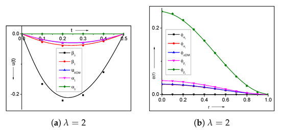
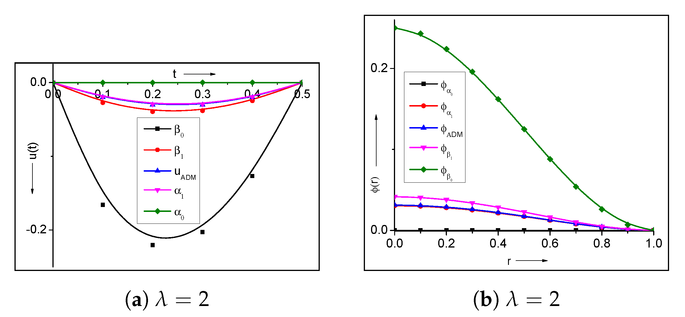
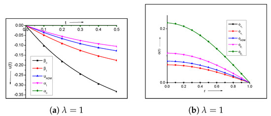
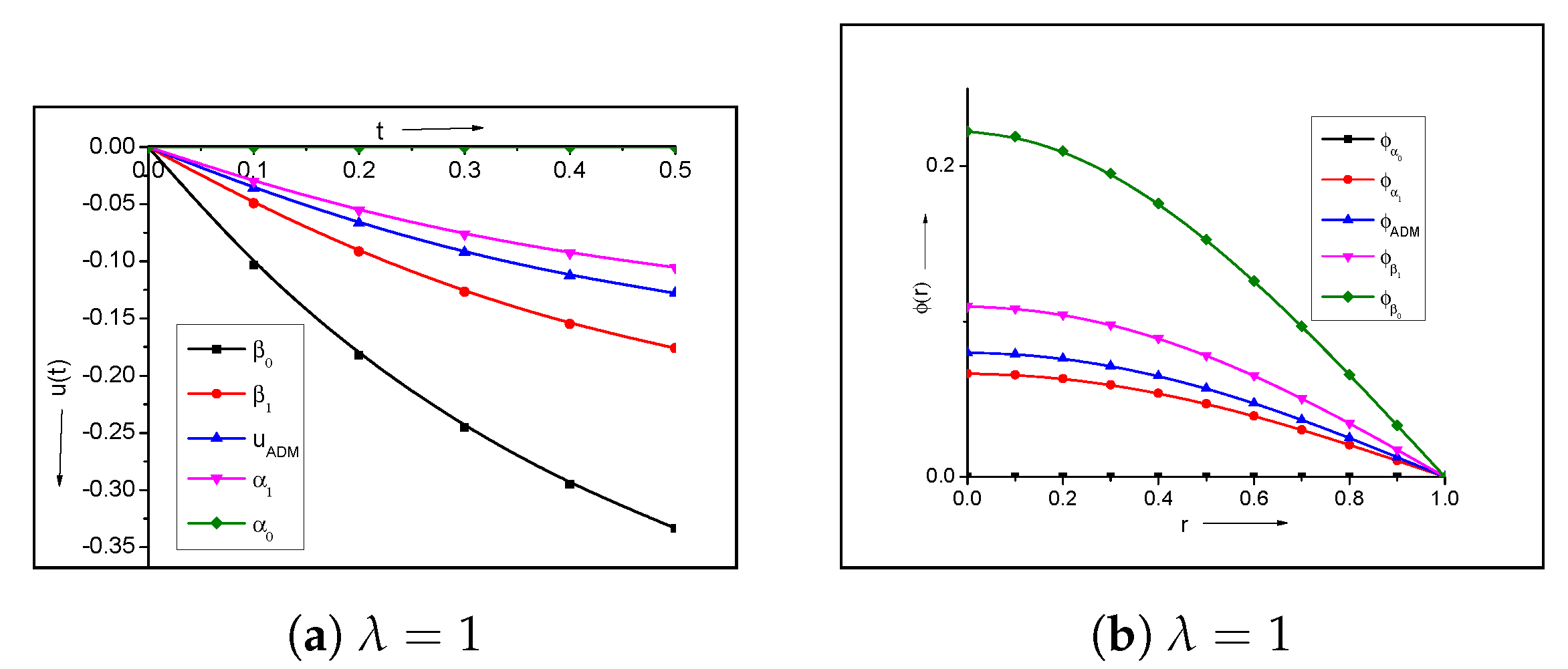
In Figure 1a, we plotted ${\beta }_0$, ${\beta }_1$, $u_{ADM}$, ${\alpha }_1$, and ${\alpha }_0$ corresponding to problem (12) for $\lambda =2$. We have seen that the lower sequence $\left\{{\beta }_n\right\}$ and upper sequence $\left\{{\alpha }_n\right\}$ always satisfies the inequality ${\beta }_n\le {\alpha }_n$. In Figure 1b, we have placed the monotone iterations of fourth-order SBVP corresponding to problem (12) for $\lambda =2$. Here, we also observed the existence of at least one solution for a fourth-order SBVP corresponding to the Dirichlet boundary condition.

Figure 1. Approximate monotone iterations of Equations (52)–(55) corresponding to problem (12) for k = −1 and $\lambda =2$.

Corresponding to problem (13): From Lemma 18, we chose the initial monotone iterations as follows:

$${\beta }_0\left(t\right)=-t\left({\displaystyle \frac{3}{2}}-\sqrt{2t}\right)\wedge {\alpha }_0\left(t\right)=0,\forall t\in [0,1].$$

(151)

The same remarks follow as discussed above.

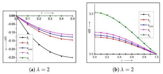
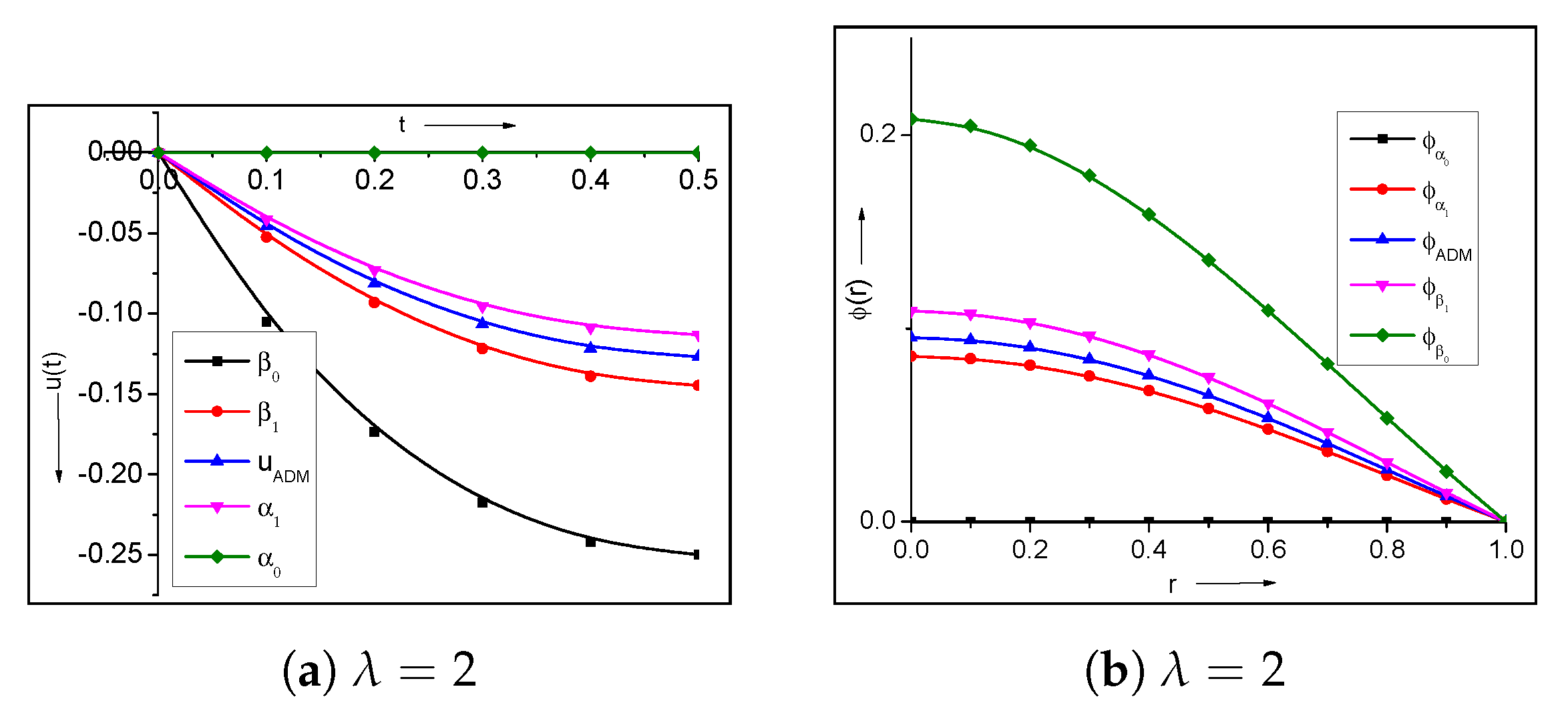
In Figure 2a,b, we present the numerical results for $k=-1$ and $\lambda =2$. We noticed that the approximate solution $u_{ADM}$ and ${\varphi }_{ADM}$ always lies between the lower sequence $\left\{{\beta }_n\right\}$ and upper sequence $\left\{{\alpha }_n\right\}$.

Figure 2. Approximate monotone iterations of Equations (52)–(55) corresponding to problem (13) for k = −1 and $\lambda =2$.

Corresponding to problem (14): Here, we consider the initial monotone iterations

$${\beta }_0\left(t\right)=-{\displaystyle \frac{2}{3}}t\left(2-\sqrt{2t}\right)\wedge {\alpha }_0\left(t\right)=0,\forall t\in [0,1].$$

(152)

We also included the same remarks as those stated above.

Monotone lower and upper iterations corresponding to the second-order and the fourth-order differential equation are plotted in Figure 3.

Figure 3. Approximate monotone iterations of Equations (52)–(55) corresponding to problem (14) for k = −1 and $\lambda =1$.

6. Conclusions

In this work, we derived some qualitative properties of the singular boundary value problems that arise in the theory of epitaxial growth. Moreover, we proved the existence of a solution and discovered a range of parameter k, for which the nonlinear problem has multiple solutions in the region $D_0$. We established the bounds of the parameter $\lambda$, from which we confirmed the nonexistence of solutions. Furthermore, the boundary value problems have multiple solutions, therefore it is challenging for researchers to obtain a suitable scheme to capture both solutions with the desired accuracy. However, we successfully developed iterative schemes and captured both solutions with a high accuracy. From Table 1, Table 2, Table 3 and Table 4, we can see that the approximate solutions computed by our proposed method converge to the exact solutions very quickly. Corresponding to the boundary conditions (7), we notice that the positive approximate solution converges to the exact positive solution very slowly (See Table 6). We verified that our numerical results matched well with our theoretical results as well as the existing numerical results [9]. We conclude that our proposed technique is relatively powerful and efficient. Furthermore, this technique is an effective tool to solve BVPs, which have multiple solutions.

References

- Barabasi, A.L.; Stanley, H.E. Fractal Concepts in Surface Growth; Cambridge University Press: Cambridge, UK, 1995. [Google Scholar]
- Lourdudoss, S.; Kjebon, O. Hybrid vapor phase epitaxy revisited. IEEE J. Sel. Top. Quantum Electron. 1997, 3, 749–767. [Google Scholar] [CrossRef] [Scilit]
- Foord, J.S.; Davies, G.J.; Tsang, W.T. Chemical Beam Epitaxy and Related Techniques; John Wiley and Sons Ltd.: Chichester, UK, 1997. [Google Scholar]
- Escudero, C. Geometric principles of surface growth. Phys. Rev. Lett. 2008, 101, 1–4. [Google Scholar] [CrossRef] [Scilit]
- Escudero, C.; Hakl, R.; Peral, I.; Torres, P.J. On radial stationary solutions to a model of non equilibrium growth. Eur. J. Appl. Math. 2013, 24, 437–453. [Google Scholar] [CrossRef] [Scilit]
- Escudero, C.; Hakl, R.; Peral, I.; Torres, P.J. Existence and nonexistence result for a singular boundary value problem arising in the theory of epitaxial growth. Math. Methods Appl. Sci. 2014, 37, 793–807. [Google Scholar] [CrossRef] [Scilit]
- Escudero, C.; Korutcheva, E. Origins of scaling relations in non equilibrium growth. J. Phys. Math. Theor. 2012, 45, 1–14. [Google Scholar]
- Verma, A.K.; Pandit, B.; Escudero, C. Numerical solutions for a class of singular boundary value problems arising in the theory of epitaxial growth. Eng. Comput. 2019, 37, 2539–2560. [Google Scholar] [CrossRef] [Scilit]
- Verma, A.K.; Pandit, B.; Agarwal, R.P. On approximate stationary radial solutions for a class of boundary value problems arising in epitaxial growth theory. J. Appl. Comput. Mech. 2019, 4, 713–734. [Google Scholar]
- Verma, A.K.; Pandit, B.; Agarwal, R.P. On multiple solutions for a fourth order nonlinear singular boundary value problems arising in epitaxial growth theory. Math. Methods Appl. Sci. 2020. [Google Scholar] [CrossRef] [Scilit]
- Cabada, A.; Cid, J.A.; Sanchez, L. Positivity and lower and upper solutions for fourth order boundary value problems. Nonlinear Anal. 2007, 67, 1599–1612. [Google Scholar] [CrossRef] [Scilit]
- Ladde, G.S.; Lakshmikantham, V.; Vatsala, A.S. Monotone Iterative Techniques for Nonlinear Differential Equations; Pitman Advance Publishing Program: Boston, MA, USA, 1985. [Google Scholar]
- Pandey, R.K.; Verma, A.K. Existence-uniqueness results for a class of singular boundary value problems-ii. J. Math. Anal. Appl. 2008, 338, 1387–1396. [Google Scholar] [CrossRef] [Scilit]
- Pandey, R.K.; Verma, A.K. Existence-uniqueness results for a class of singular boundary value problems arising in physiology. Nonlinear Anal. 2008, 9, 40–52. [Google Scholar] [CrossRef] [Scilit]
- Pandey, R.K.; Verma, A.K. On solvability of derivative dependent doubly singular boundary value problems. J. Appl. Math. Comput. 2010, 33, 489–511. [Google Scholar] [CrossRef] [Scilit]
- Pandey, R.K.; Verma, A.K. Monotone method for singular bvp in the presence of upper and lower solutions. Appl. Math. Comput. 2010, 215, 3860–3867. [Google Scholar] [CrossRef] [Scilit]
- Wang, G.; Agarwal, R.P.; Cabada, A. Existence results and the monotone iterative technique for systems of nonlinear fractional differential equations. Appl. Math. Lett. 2012, 25, 1019–1024. [Google Scholar] [CrossRef] [Scilit]
- Agarwal, R.; O’Regan, D.; Hristova, S. Monotone iterative technique for the initial value problem for differential equations with non-instantaneous impulses. Appl. Math. Comput. 2017, 298, 45–56. [Google Scholar] [CrossRef] [Scilit]
- Xue, T.; Liu, W.; Shen, T. Extremal solutions for p-laplacian boundary value problems with the right-handed riemann-liouville fractional derivative. Math. Methods Appl. Sci. 2019, 42, 4394–4407. [Google Scholar] [CrossRef] [Scilit]
- Mittal, R.C.; Nigam, R. Solution of a class of singular boundary value problems. Numer. Algorithm 2008, 47, 169–179. [Google Scholar] [CrossRef] [Scilit]
- Odibat, Z.; Momani, S. A reliable treatment of homotopy perturbation method for klein-gordon equations. Phys. Lett. A 2007, 365, 351–357. [Google Scholar] [CrossRef] [Scilit]
- Abbasbandy, S. Numerical solutions of the integral equations: Homotopy perturbation method and adomian’s decomposition method. Appl. Math. Comput. 2006, 173, 493–500. [Google Scholar] [CrossRef] [Scilit]
- Babolian, E.; Davari, A. Numerical implementation of adomian decomposition method for linear volterra integral equations of the second kind. Appl. Math. Comput. 2005, 165, 223–227. [Google Scholar] [CrossRef] [Scilit]
- Maleknejad, K.; Hadizadeh, M. A new computational method for volterra-fredholm integral equations. Comput. Math. Appl. 1999, 37, 1–8. [Google Scholar] [CrossRef] [Scilit]
- Abdulaziz, O.; Hashima, I.; Momani, S. Application of homotopy perturbation method to fractional ivps. J. Comput. Appl. Math. 2008, 216, 574–584. [Google Scholar] [CrossRef] [Scilit]
- Hu, Y.; Luo, Y.; Lua, Z. Analytical solution of the linear fractional differential equation by adomian decomposition method. J. Comput. Appl. Math. 2008, 215, 220–229. [Google Scholar] [CrossRef] [Scilit]
- Grzymkowski, R.; Pleszczyński, M.; Słota, D. Comparing the Adomian decomposition methodand the Runge–Kutta method for solutions of theStefan problem. Int. J. Comput. Math. 2006, 83, 409–417. [Google Scholar] [CrossRef] [Scilit]
- Grzymkowski, R.; Słota, D. Stefan problem solved by Adomian decomposition method. Int. J. Comput. Math. 2005, 82, 851–856. [Google Scholar] [CrossRef] [Scilit]
- Grzymkowski, R.; Słota, D. One—Phase Inverse Stefan Problem Solved Adomian Decomposition Method. Comput. Math. Appl. 2006, 51, 33–40. [Google Scholar] [CrossRef] [Scilit]
- Grzymkowski, R.; Pleszczyński, M.; Słota, D. The Two-Phase Stefan Problem Solved by the Adomian Decomposition Method. In Proceedings of the 15th IASTED International Conference Applied Simulation and Modelling, Rhodes, Greece, 26–28 June 2006. [Google Scholar]
- Verma, A.K.; Pandit, B.; Agarwal, R.P. Existence and nonexistence results for a class of fourth-order coupled singular boundary value problems arising in the theory of epitaxial growth. Math. Methods Appl. Sci. 2020. [Google Scholar] [CrossRef] [Scilit]
- Hayani, W.A. Adomian decomposition method with green’s function for sixth order boundary value problems. Comput. Math. Appl. 2011, 61, 1567–1575. [Google Scholar] [CrossRef] [Scilit]
- Singh, R.; Kumar, J. The adomian decomposition method with green’s function for solving nonlinear singular boundary value problems. J. Appl. Math. Comput. 2014, 44, 397–416. [Google Scholar] [CrossRef] [Scilit]
- Noeiaghdam, S.; Sidorov, D.; Wazwaz, A.M.; Sidorov, N.; Sizikov, V. The Numerical Validation of the Adomian Decomposition Method for Solving Volterra Integral Equation with Discontinuous Kernels Using the CESTAC Method. Mathematics 2021, 9, 260. [Google Scholar] [CrossRef] [Scilit]
- Verma, A.K.; Pandit, B.; Verma, L.; Agarwal, R.P. A review on a class of second order nonlinear singular BVPs. Mathematics 2020, 8, 1045. [Google Scholar] [CrossRef] [Scilit]
- Verma, A.K.; Pandit, B.; Agarwal, R.P. Continuous Galerkin Method and Lane-Emden Equations. Adv. Math. Sci. Appl. 2021, 30, 39–64. [Google Scholar]
- Cabada, A. An overview on the lower and upper solutions method with nonlinear boundary value problem. Bound. Value Probl. 2011, 2011, 893753. [Google Scholar] [CrossRef] [Scilit]
- Ghorbani, A. Beyond adomian polynomials: He polynomials. Chaos Solitons Fractals 2009, 39, 1486–1492. [Google Scholar] [CrossRef] [Scilit]
- Singh, R.; Wazwaz, A.M. An efficient algorithm for solving coupled Lane-Emden boundary value problems in Catalytic diffusion reactions: The homotopy analysis method. Commun. Math. Comput. Chem. 2019, 81, 785–800. [Google Scholar]
Publisher’s Note: MDPI stays neutral with regard to jurisdictional claims in published maps and institutional affiliations. |
© 2021 by the authors. Licensee MDPI, Basel, Switzerland. This article is an open access article distributed under the terms and conditions of the Creative Commons Attribution (CC BY) license (https://creativecommons.org/licenses/by/4.0/).