Numerical Solution of the Boundary Value Problems Arising in Magnetic Fields and Cylindrical Shells

Abstract

This paper is devoted to the study of the Cubic B-splines to find the numerical solution of linear and non-linear 8th order BVPs that arises in the study of astrophysics, magnetic fields, astronomy, beam theory, cylindrical shells, hydrodynamics and hydro-magnetic stability, engineering, applied physics, fluid dynamics, and applied mathematics. The recommended method transforms the boundary problem to a system of linear equations. The algorithm we are going to develop in this paper is not only simply the approximation solution of the 8th order BVPs using Cubic-B spline but it also describes the estimated derivatives of 1st order to 8th order of the analytic solution. The strategy is effectively applied to numerical examples and the outcomes are compared with the existing results. The method proposed in this paper provides better approximations to the exact solution.

1. Introduction

It is frequently significant in practice to find estimated illustrations of physical data by comparatively simple mathematical functions. The approximating functions are typically compulsory to fulfill definite standards involving to precision and smoothness. Earlier, polynomials have regularly been used for such mission, but it had been accepted that there were numerous kinds of data set for which polynomial approximations were unacceptable in that a very high degree may be mandatory to attain the essential accurateness.

To overcome such complications attention has turned to the use of piece-wise polynomials or spline functions. Spline only means a piece-wise polynomial of degree k that is continuously differentiable $k-1$ times. Spline interpolation is a formula of interpolation wherever the interpolate is a different kind of piece-wise polynomial called spline. Spline interpolation escapes the problem of Runge’s phenomenon, in which oscillation happens among points when interpolating using high degree polynomials. Cubic Spline interpolation is a different type of spline interpolation which is utilized very frequently to escape the problem of Runge’s phenomenon. That technique provides an interpolating polynomial which is evener and has lesser error than former interpolating polynomials such as Lagrange polynomial and Newton polynomial.

A B-spline is a linear combination of a set of basis functions that are determined by the number and location of specified knots or cut-points. Splines are signified here in forms of a basis (as linear combination of certain basis polynomials such as Chebyshev or Legendre polynomials). B-splines are assembled by polynomial pieces linked at a set of nodes. When the nodes are specified, B-splines can be estimated recursively for any degree of the polynomial by using a mathematically steady procedure.

Here in this paper linear and non-linear 8th order BVP’s are discussed that ascends in the study of astrophysics, astronomy, beam theory and long wave theory, hydrodynamics and hydro-magnetic stability, engineering, applied physics, fluid dynamics, and applied mathematics.

Let us consider a linear 8th order BVP

$$\begin{array}{c}{w}^{(8)}(z)+a_1(z)w^{(7)}(z)+a_2(z)w^{(6)}(z)+a_3(z)w^{(5)}(z)+a_4(z)w^{(4)}(z)+a_5(z)w^{(3)}(z)\hfill \\ +a_6(z)w^{(2)}(z)+a_7(z)w^{(1)}(z)+a_8(z)w(z)=f(z),z\in [a,b]\hfill \end{array}$$

(1)

Consider a 8th order non-linear BVP

$$\begin{array}{c}{w}^{(8)}(z)=f(z,w(z),w^{(1)}(z),w^{(2)}(z),w^{(3)}(z),w^{(4)}(z),w^{(5)}(z),w^{(6)}(z),w^{(7)}(z)),z\in \left[a,b\right]\hfill \end{array}$$

(2)

with boundary conditions

$$\begin{array}{cccc}w(a)={\alpha }_0,\hfill & w^{(1)}(a)={\alpha }_1,\hfill & w^{(2)}(a)={\alpha }_2,\hfill & w^{(3)}(a)={\alpha }_3,\hfill \\ w(b)={\beta }_0,\hfill & w^{(1)}(b)={\beta }_1,\hfill & w^{(2)}(b)={\beta }_2,\hfill & w^{(3)}(b)={\beta }_3,\hfill \end{array}$$

(3)

where ${\alpha }_j$ and ${\beta }_j$ $(j=0,1,\dots ,3)$ are given real constants, $(a_i(z);i=1,2,\dots ,8)$ and $f$ is continuous on the given interval $[a,b]$.

Theorems which list the conditions for the existence and uniqueness of solution for those type of problems have been deliberated in a inclusive review in a book [1], however no numerical approaches are contained within for resolving BVP’s of higher order.

In [2] the authors presented the solution of 8th order BVP’s using kernel space, In [3] ninth order non-polynomial spline functions were used for the solution of 8th order BVP’s. In [4] the authors explored torsional vibration of uniform beams concerning 8th order differential equation and in [5] the authors discussed finite difference method to solve the 8th order BVP’s. In [6], B-spline interpolation was compared with finite difference, finite element and finite volume methods which was applied to two-point BVP’s.

Chandrasekhar [7] conveyed if an infinite horizontal layer of fluid is heated from below and is in the act of rotation, instability sets in. When the instability sets in as over-stability, it is modeled by an 8th-order ordinary differential equation. Convergence of odd degree spline was argued in [8]. Cubic-B spline solution of a nonlinear system of second order BVP’s was discussed in [9]. In [10,11,12], some numerical methods like Spectral Galerkin method and Legendre Galerkin method for solving special 8th-order linear BVP’s were discussed.

In [13], the authors found a new method using Cubic B-spline for the solution of linear 4th order BVP’s. Error bounds for spline interpolation was found in [14,15]. In [16,17,18] the authors proposed optimal Homotopy asymptotic method and homotopy perturbation method for 8th order BVP’s linear and non-linear problems. In [19] the authors presented the solution for 8th order BVP’s using ADM. Cubic B-spline Solution of Nonlinear Sixth Order BVP’s is discussed in [20]. In [21], the authors found new Cubic B-Spline for the solution of linear 5th order BVP’s. So far cubic B-Spline is not discussed for seventh and higher order linear and nonlinear BVP’s as basis functions.

Reproducing kernel space was used for solution of a class nonlinear equations in [22]. In [23,24] the authors projected the solution for the for 8th order BVP’s using Generalized Differential Quadrature and modified decomposition method. In [25,26,27,28] used Exp-function method, Homotopy perturbation method and Variational iteration method for solving higher-order non-linear BVP’s. The equations for the equilibrium for an orthotropic thin circular cylindrical shell found in [29].

Petrov-Galerkin method was used in [30] and Haar wavelet collocation method was used in [31] for solving 8th order BVP’s. The cylindrical shell equations are derived in [32]. Shen [33] derived the 8th order differential equation by bending and axial vibrations of an elastic beam. In [34,35,36,37] many authors built-up Quintic B-splines Collocation method, Sextic B-Spline Collocation Method, Galerkin Method with Quintic B-splines and Galerkin method with Septic B-splines for 8th order BVP. Wazwaz [38] used modified decomposition method to solve special 8th-order BVP’s.

2. Fundamentals of Cubic B-Splines

Let the given interval $[a,b]$ be divided into sub intervals of equal length such that

$$\mathsf{\Omega }=[a,b]$$

and

$${\mathsf{\Omega }}_i=z_i=a+ih,$$

for $i=0,1,2,\cdots ,n$ where $h=\frac{b-a}{n}$.

Let us consider $S^3(\mathsf{\Omega })=\{p(t)\in C^2(\mathsf{\Omega })\}$ where $p(t)$ denotes the set of uni variate cubic polynomial on sub-interval $(z_i,z_{i+1})$. The basis function is defined as

$$B_{-1}(z)=\frac{1}{6h^3}\left\{\begin{array}{c}{(z_1-z)}^3,ifz\in [z_0,z_1]\hfill \\ 0,\mathrm{otherwise}\hfill \end{array}\right.$$

$$B_0(z)=\frac{1}{6h^3}\left\{\begin{array}{c}{h}^3+3h^2(z_1-z)+3h{(z_1-z)}^2-3{(z_1-z)}^3,ifz\in [z_0,z_1]\hfill \\ {(z_2-z)}^{3}ifz\in [z_1,z_2]\hfill \\ 0,\mathrm{otherwise}\hfill \end{array}\right.$$

$$B_1(z)=\frac{1}{6h^3}\left\{\begin{array}{c}{h}^3+3h^2(z-z_0)+3h{(z-z_0)}^2-3{(z-z_0)}^3,ifz\in [z_0,z_1]\hfill \\ h^3+3h^2(z_2-z)+3h{(z_2-z)}^2-3{(z_2-z)}^3,ifz\in [z_1,z_2]\hfill \\ {(z_3-z)}^{3}ifz\in [z_1,z_2]\hfill \\ 0,\mathrm{otherwise}\hfill \end{array}\right.$$

$$B_i(z)=\frac{1}{6h^3}\left\{\begin{array}{c}{(z-z_{i-2})}^{3}ifz\in [z_{i-2},z_{i-1}]\hfill \\ h^3+3h^2(z-z_{i-1})+3h{(z-z_{i-1})}^2-3{(z-z_{i-1})}^3,ifz\in [z_{i-1},z_i]\hfill \\ h^3+3h^2(z_{i+1}-z)+3h{(z_{i+1}-z)}^2-3{(z_{i+1}-z)}^3,ifz\in [z_i,z_{i+1}]\hfill \\ {(z_{i+2}-z)}^{3}ifz\in [z_{i+1},z_{i+2}]\hfill \\ 0,\mathrm{otherwise}\hfill \end{array}\right.$$

for $i=0,1,\dots ,n$. Since each $B_i(z)$ is similarly a piece-wise cubic with nodes at $\mathsf{\Omega }$, so collectively $B_i(z)\in S_3(\mathsf{\Omega })$. Let $\mathsf{\Psi }=\{B_{-1},B_0,B_1,\dots ,B_{n+1}\}$ and let $B_3(\mathsf{\Omega })=span\mathsf{\Psi }$. The functions in $\mathsf{\Psi }$ are linearly independent on $[a,b]$, thus $B_3(\mathsf{\Omega })$ is $(n+3)$-dimensional and $B_3(\mathsf{\Omega })=S_3(\mathsf{\Omega })$. Let $S(z_i)$ be the Cubic B-spline interpolating function at the nodal points and $S(z_i)\in B_3(\mathsf{\Omega })$. Then $S(z_i)$ can be written as

$$S(z_i)=\sum _{i=-1}^{n+1}{\ell }_1{B}_i(z_i).$$

(4)

The values of $B(z)$, $B^{(1)}(z)$ and $B^{(2)}(z)$ at the nodes are listed in Table 1.

Table 1. Values of $B(z)$, $B^{(1)}(z)$ and $B^{(2)}(z)$ at the nodes.

	${\mathit{B}}_{\mathit{i}}(\mathit{z})$	${\mathit{B}}_{\mathit{i}}{}^{(1)}(\mathit{z})$	${\mathit{B}}_{\mathit{i}}{}^{(2)}(\mathit{z})$
$z_{i-2}$	0	0	0
$z{}_{i-1}$	1/6	$1/2h$	$1/h{}^2$
$z{}_i$	4/6	0	−2/$h{}^2$
$z{}_{i+1}$	1/6	−1/2h	1/$h{}^2$
$z{}_{i-2}$, $z{}_{i+2}$ and all others	0	0	0

For an assumed function $w(z_i)$ there will be a Cubic B-spline satisfying the interpolating conditions:

$$s(z_i)=w(z_i),$$

(5)

where $i=0,1,\dots ,n,$ and

$$s(a)=w(a),s(b)=w(b)$$

(6)

and

$$s^{(1)}(a)=w^{(1)}(a),s^{(1)}(b)=w^{(1)}(b)$$

(7)

Let $m_i=s^{(1)}(z_i)$ and $M_i=s^{(2)}(z_i)$ then from [20]

$$m_i=s^{(1)}(z_i)=w^{(2)}(z_i)-\frac{1}{180}{h}^4{w}^{(6)}(z_i)+O(h^6).$$

(8)

$$M_i=s^{(2)}(z_i)=w^{(2)}(z_i)-\frac{1}{12}{h}^2{w}^{(4)}(z_i)+\frac{1}{360}{h}^4{w}^{(6)}(z_i)+O(h^6).$$

(9)

$M_i$ can be used to calculate the numerical difference formulas for $w^{(3)}(z_i),w^{(4)}(z_i)$ where $i=1,2,\dots ,n-1$, $w^{(5)}(z_i),w^{(6)}(z_i)$ where $i=2,\dots ,n-2$ and $w^{(7)}(z_i),w^{(8)}(z_i)$ where $i=3,\dots ,n-3$ as follows, wherever the errors are acquired by the Taylor series expansion

$$\frac{M_{i+1}-M_{i-1}}{2h}=\frac{s^3(z_{i-})-s^3(z_{i+})}{2}=w^{(3)}(z_i)+\frac{1}{12}{h}^2{w}^{(5)}(z_i)+O(h^4)$$

(10)

From [16,19],

$$\frac{M_{i+1}-2M_i+M_{i-1}}{h^2}=\frac{s^3(z_{i+})-s^3(z_{i-})}{h}=w^{(4)}(z_i)-\frac{1}{720}{h}^4{w}^{(8)}(z_i)+O(h^6)$$

(11)

$$\frac{M_{i+2}-2M_{i+1}+2M_{i-1}-M_{i-2}}{2h^3}=w^{(5)}(z_i)+O(h^2)$$

(12)

And from [18],

$$w^{(6)}(z_i)=\frac{w_{i+1}^{(4)}(z_i)-2w_i^{(4)}(z_i)+w_{i-1}^{(4)}(z_i)}{h^2}$$

(13)

$$\frac{M_{i+2}-4M_{i+1}+6M_i-4M_{i-1}+M_{i-2}}{h^4}=w^{(6)}(z_i)+O(h^2)$$

(14)

Following the above the Taylor series expansion for $w^{(7)}(z_i)$ at the selected collocation points with central difference the authors of this paper have found that

$$w^{(7)}(z_i)=\frac{w_{i+2}^{(4)}(z_i)-2w_{i+1}^{(4)}(z_i)+2w_{i-1}^{(4)}(z_i)-w_{i-2}^{(4)}(z_i)}{2h^3}$$

(15)

$$\frac{M_{i+3}-4M_{i+2}+5M_{i+1}-5M_{i-1}+4M_{i-2}+M_{i-3}}{2h^5}=w^{(7)}(z_i)+O(h^2)$$

(16)

3. Cubic-B Spline Solutions of 8th Order BVP

Following the above the Taylor series expansion for $w^{(8)}(z_i)$ at the selected collocation points with central difference, we have

$$w^{(8)}(z_i)=\frac{w_{i+2}^{(4)}(z_i)-4w_{i+1}^{(4)}(z_i)+6w_i^{(4)}(z_i)-4w_{i-1}^{(4)}(z_i)+w_{i-2}^{(4)}(z_i)}{h^4}$$

(17)

From Equation (11) we have

$$\begin{array}{c}\frac{M_{i-1}-2M_{i-2}+M_{i-3}}{h^2}=w^{(4)}(z_{i-2})-\frac{1}{720}{h}^2{w}^{(8)}(z_{i-2})+O(h^6)\hfill \\ \frac{M_i-2M_{i-1}+M_{i-2}}{h^2}=w^{(4)}(z_{i-1})-\frac{1}{720}{h}^2{w}^{(8)}(z_{i-1})+O(h^6)\hfill \\ \frac{M_{i+2}-2M_{i+1}+M_i}{h^2}=w^{(4)}(z_{i+1})-\frac{1}{720}{h}^2{w}^{(8)}(z_{i+1})+O(h^6)\hfill \\ \frac{M_{i+3}-2M_{i+2}+M_{i+1}}{h^2}=w^{(4)}(z_{i+2})-\frac{1}{720}{h}^2{w}^{(8)}(z_{i+2})+O(h^6)\hfill \end{array}$$

(18)

Using Equations (11) and (18) in Equation (17), we have

$$\frac{M_{i+3}-6M_{i+2}+15M_{i+1}-20M_i+15M_{i-1}-6M_{i-2}+M_{i-3}}{h^6}=w^{(8)}(z_i)+O(h^2)$$

(19)

As $M_i=\frac{{\ell }_{i+1}-2{\ell }_i+{\ell }_{i-1}}{h^2}$ using this we have

$$M_{i-1}=\frac{{\ell }_i-2{\ell }_{i-1}+{\ell }_{i-2}}{h^2},M_{i-2}=\frac{{\ell }_{i-1}-2{\ell }_{i-2}+{\ell }_{i-3}}{h^2},M_{i-3}=\frac{{\ell }_{i-2}-2{\ell }_{i-3}+{\ell }_{i-4}}{h^2}$$

$$M_{i+1}=\frac{{\ell }_{i+2}-2{\ell }_{i+1}+{\ell }_i}{h^2},M_{i+2}=\frac{{\ell }_{i+3}-2{\ell }_{i+2}+{\ell }_{i+1}}{h^2},M_{i+3}=\frac{{\ell }_{i+4}-2{\ell }_{i+3}+{\ell }_{i+2}}{h^2}$$

so Equation (19) becomes

$$\begin{array}{c}{w}^{(8)}(z_i)=\frac{1}{h^6}(\frac{{\ell }_{i+4}-2{\ell }_{i+3}+{\ell }_{i+2}}{h^2}-6(\frac{{\ell }_{i+3}-2{\ell }_{i+2}+{\ell }_{i+1}}{h^2})+15(\frac{{\ell }_{i+2}-2{\ell }_{i+1}+{\ell }_i}{h^2})\hfill \\ -20(\frac{{\ell }_{i+1}-2{\ell }_i+{\ell }_{i-1}}{h^2})+15(\frac{{\ell }_i-2{\ell }_{i-1}+{\ell }_{i-2}}{h^2})-6(\frac{{\ell }_{i-1}-2{\ell }_{i-2}+{\ell }_{i-3}}{h^2})+\frac{{\ell }_{i-2}-2{\ell }_{i-3}+{\ell }_{i-4}}{h^2})\hfill \end{array}$$

$$\begin{array}{c}{w}^{(8)}(z_i)=\frac{1}{h^8}({\ell }_{i+4}-2{\ell }_{i+3}+{\ell }_{i+2}-6({\ell }_{i+3}-2{\ell }_{i+2}+{\ell }_{i+1})+15({\ell }_{i+2}-2{\ell }_{i+1}+{\ell }_i)-20({\ell }_{i+1}\hfill \\ -2{\ell }_i+{\ell }_{i-1})+15({\ell }_i-2{\ell }_{i-1}+{\ell }_{i-2})-6({\ell }_{i-1}-2{\ell }_{i-2}+{\ell }_{i-3})+{\ell }_{i-2}-2{\ell }_{i-3}+{\ell }_{i-4})\hfill \end{array}$$

$$w^{(8)}(z_i)=s^{(8)}(z_i)=\frac{{\ell }_{i+4}-8{\ell }_{i+3}+28{\ell }_{i+2}-56{\ell }_{i+1}+70{\ell }_i-56{\ell }_{i-1}+28{\ell }_{i-2}-8{\ell }_{i-3}+{\ell }_{i-4}}{h^8}$$

Using of Table 1 and above equations, we get estimate values of $w(z)$ and its all derivatives from 1st to 8th at the nodes as

$$\left.\begin{array}{c}w(z_i)=s(z_i)=\frac{{\ell }_{i-1}+4{\ell }_i+{\ell }_{i+1}}{6}\hfill \\ w^{(1)}(z_i)=s^{(1)}(z_i)=\frac{{\ell }_{i+1}-{\ell }_{i-1}}{2h}\hfill \\ w^{(2)}(z_i)=s^{(2)}(z_i)=\frac{{\ell }_{i+1}-2{\ell }_i+{\ell }_{i-1}}{h^2}\hfill \\ w^{(3)}(z_i)=s^{(3)}(z_i)=\frac{{\ell }_{i+2}-2{\ell }_{i+1}+2{\ell }_{i-1}-{\ell }_{i-2}}{2h^3}\hfill \\ w^{(4)}(z_i)=s^{(4)}(z_i)=\frac{{\ell }_{i+2}-4{\ell }_{i+1}+6{\ell }_i-4{\ell }_{i-1}+{\ell }_{i-2}}{h^4}\hfill \\ w^{(5)}(z_i)=s^{(5)}(z_i)=\frac{{\ell }_{i+3}-4{\ell }_{i+2}+5{\ell }_{i+1}+5{\ell }_{i-1}+4{\ell }_{i-2}-{\ell }_{i-3}}{2h^5}\hfill \\ w^{(6)}(z_i)=s^{(6)}(z_i)=\frac{{\ell }_{i+3}-6{\ell }_{i+2}+15{\ell }_{i+1}-20{\ell }_i+15{\ell }_{i-1}-6{\ell }_{i-2}+{\ell }_{i-3}}{h^6}\hfill \\ w^{(7)}(z_i)=s^{(7)}(z_i)=\frac{{\ell }_{i+4}-6{\ell }_{i+3}+14{\ell }_{i+2}-14{\ell }_{i+1}+14{\ell }_{i-1}-14{\ell }_{i-2}+6{\ell }_{i-3}-{\ell }_{i-4}}{2h^7}\hfill \\ w^{(8)}(z_i)=s^{(8)}(z_i)=\frac{{\ell }_{i+4}-8{\ell }_{i+3}+28{\ell }_{i+2}-56{\ell }_{i+1}+70{\ell }_i-56{\ell }_{i-1}+28{\ell }_{i-2}-8{\ell }_{i-3}+{\ell }_{i-4}}{h^8}\hfill \end{array}\right\}$$

(20)

4. Application of Cubic B Spline on Linear 8th Order BVP’s

Then Equation (1) at the nodes becomes:

$$\begin{array}{c}{w}^{(8)}(z_i)+a_1(z_i)w^{(7)}(z_i)+a_2(z_i)w^{(6)}(z_i)+a_3(z_i)w^{(5)}(z_i)+a_4(z_i)w^{(4)}(z_i)+a_5(z_i)w^{(3)}(z_i)\hfill \\ +a_6(z_i)w^{(2)}(z_i)+a_7(z_i)w^{(1)}(z_i)+a_8(z_i)w(z_i)=f(z_i),z_i\in [a,b]\hfill \end{array}$$

(21)

Using Equation (20) in Equation (21), we have

$$\begin{array}{c}\frac{1}{h^8}({\ell }_{i+4}-8{\ell }_{i+3}+28{\ell }_{i+2}-56{\ell }_{i+1}+70{\ell }_i-56{\ell }_{i-1}+28{\ell }_{i-2}-8{\ell }_{i-3}+{\ell }_{i-4})+a_1(z{}_i)\frac{1}{2h^7}\hfill \\ ({\ell }_{i+4}-6{\ell }_{i+3}+14{\ell }_{i+2}-14{\ell }_{i+1}+14{\ell }_{i-1}-14{\ell }_{i-2}+6{\ell }_{i-3}-{\ell }_{i-4})+a_2(z{}_i)\frac{1}{h^6}({\ell }_{i+3}-6{\ell }_{i+2}\hfill \\ +15{\ell }_{i+1}-20{\ell }_i+15{\ell }_{i-1}-6{\ell }_{i-2}+{\ell }_{i-3})+a_3(z{}_i)\frac{1}{2h^5}({\ell }_{i+3}-4{\ell }_{i+2}+5{\ell }_{i+1}+5{\ell }_{i-1}+4{\ell }_{i-2}\hfill \\ -{\ell }_{i-3})+a_4(z{}_i)\frac{1}{h^4}({\ell }_{i+2}-4{\ell }_{i+1}+6{\ell }_i-4{\ell }_{i-1}+{\ell }_{i-2})+a_5(z{}_i)\frac{1}{2h^3}({\ell }_{i+2}-2{\ell }_{i+1}+2{\ell }_{i-1}\hfill \\ -{\ell }_{i-2})+a_6(z{}_i)\frac{1}{h^2}({\ell }_{i+1}-2{\ell }_i+{\ell }_{i-1})+a_7(z{}_i)\frac{1}{2h}({\ell }_{i+1}-{\ell }_{i-1})+a_8(z{}_i)\frac{1}{6}({\ell }_{i-1}+4{\ell }_i\hfill \\ +{\ell }_{i+1})=f_i(z{}_i),z\in \left[a,b\right]\hfill \end{array}$$

after simplifying, we have

$$\begin{array}{c}6({\ell }_{i+4}-8{\ell }_{i+3}+28{\ell }_{i+2}-56{\ell }_{i+1}+70{\ell }_i-56{\ell }_{i-1}+28{\ell }_{i-2}-8{\ell }_{i-3}+{\ell }_{i-4})+3h{a}_1(z{}_i)({\ell }_{i+4}\hfill \\ -6{\ell }_{i+3}+14{\ell }_{i+2}-14{\ell }_{i+1}+14{\ell }_{i-1}-14{\ell }_{i-2}+6{\ell }_{i-3}-{\ell }_{i-4})+6h^2{a}_2(z{}_i)({\ell }_{i+3}-6{\ell }_{i+2}+15\hfill \\ {\ell }_{i+1}-20{\ell }_i+15{\ell }_{i-1}-6{\ell }_{i-2}+{\ell }_{i-3})+3h^3{a}_3(z{}_i)({\ell }_{i+3}-4{\ell }_{i+2}+5{\ell }_{i+1}+5{\ell }_{i-1}+4{\ell }_{i-2}-{\ell }_{i-3})\hfill \\ +6h^4{a}_4(z{}_i)({\ell }_{i+2}-4{\ell }_{i+1}+6{\ell }_i-4{\ell }_{i-1}+{\ell }_{i-2})+3h^5{a}_5(z{}_i)({\ell }_{i+2}-2{\ell }_{i+1}+2{\ell }_{i-1}-{\ell }_{i-2})\hfill \\ +6h^6{a}_6(z{}_i)({\ell }_{i+1}-2{\ell }_i+{\ell }_{i-1})+3h^7{a}_7(z{}_i)({\ell }_{i+1}-{\ell }_{i-1})+h^8{a}_8(z{}_i)({\ell }_{i-1}+4{\ell }_i+{\ell }_{i+1})\hfill \\ =6h^8{f}_i(z{}_i),z\in \left[a,b\right]\hfill \end{array}$$

(22)

where $f_i=f(z_i)$ be the values of $f(z)$ at the nodes $z_i(i=0,1,\dots ,n)$. By solving Equation (22) we will have a linear system of $(n-5)$ linear equations $(i=2,3,\dots ,n-2)$ with $(n+3)$ unknowns $l_i$ where $(i=-1,0,1,\dots ,n+1)$, so eight more equations are desirable. By the boundary conditions at $z=a$, we will have four equations:

$$\begin{array}{c}w(z_0)={\alpha }_0\Rightarrow {\ell }_{-1}+4{\ell }_0+{\ell }_1=6{\alpha }_0\hfill \\ w^{(1)}(z_0)={\alpha }_1\Rightarrow -{\ell }_{-1}+{\ell }_1=2{\alpha }_{1}h\hfill \\ w^{(2)}(z_0)={\alpha }_2\Rightarrow {\ell }_{-1}-2{\ell }_0+{\ell }_1={\alpha }_2{h}^2\hfill \\ w^{(3)}(z_0)={\alpha }_3\Rightarrow {\ell }_2-2{\ell }_1+2{\ell }_{-1}-{\ell }_{-2}=2{\alpha }_3{h}^3\hfill \end{array}$$

(23)

if we notice Equation (23), we found a new unknown ${\ell }_{-2}$, to find this unknown we will have an equation from Equation (22) at $i=1$ Similarly for $z=b$, we will have four equations:

$$\begin{array}{c}w\left(z_n\right)={\beta }_0\Rightarrow {{\ell }_{n-}}_1+4{\ell }_n+{\ell }_{n+1}=6{\beta }_0\hfill \\ w^{(1)}(z_n)={\beta }_1\Rightarrow -{\ell }_{n-1}+{\ell }_{n+1}=2{\beta }_{1}h\hfill \\ w^{(2)}(z_n)={\beta }_2\Rightarrow {\ell }_{n-1}-2{\ell }_n+{\ell }_{n+1}={\beta }_2{h}^2\hfill \\ w^{(3)}(z_n)={\beta }_3\Rightarrow {\ell }_{n+2}-2{\ell }_{n+1}+2{\ell }_{n-1}-{\ell }_{n-2}=2{\beta }_3{h}^3\hfill \end{array}$$

(24)

if we notice Equation (24), we found a new unknown ${\ell }_{n+2}$, to find this unknown we will have an equation from Equation (22) at $i=n-1$. From Equations (23) and (24) we will have eight equations. Neglecting the order of the error terms, the approximate solution $w(z_i)=s(z_i)={\sum }_{i=-1}^{n+1}{\ell }_i{B}_i(z_i)$ can be found by solving the above system of $(n+5)$ linear equations in $(n+5)$ unknowns ${\ell }_{-2}$, ${\ell }_{-1}$, ${\ell }_0$, …, ${\ell }_{n+2}$ using the Equations (22)–(24).

5. Application of Cubic B Spline on Non-Linear 8th Order BVP’s

Then Equation (2) at the nodes becomes:

$$\begin{array}{c}{w}^{(8)}(z{}_i)=f(z{}_i,w(z{}_i),w^{(1)}(z{}_i),w^{(2)}(z{}_i),w^{(3)}(z{}_i),w^{(4)}(z{}_i),w^{(5)}(z{}_i),w^{(6)}(z{}_i),w^{(7)}(z{}_i))\hfill \end{array}$$

(25)

Using Equation (20) in Equation (25), we have

$$\begin{array}{c}\frac{1}{h^8}(l_{i+4}-8{l_{i+3}+28l}_{i+2}{-56l_{i+1}+70l_i-56l_{i-1}+28l_{i-2}-8l_{i-3}+l}_{i-4})=f_i(z{}_i,\frac{1}{6}(l_{i-1}\hfill \\ +4l_i+l_{i+1}),\frac{1}{2h}(l_{i+1}-l_{i-1}),\frac{1}{h^2}(l_{i+1}-2l_i+l_{i-1}),\frac{1}{2h^3}(l_{i+2}-2l_{i+1}+2l_{i-1}-l_{i-2}),\hfill \\ \frac{1}{h^4}(l_{i+2}-4l_{i+1}+6l_i-4l_{i-1}+l_{i-2}),\frac{1}{2h^5}(l_{i+3}-4l_{i+2}+5l_{i+1}+5l_{i-1}+4l_{i-2}-l_{i-3}),\hfill \\ \frac{1}{h^6}(l_{i+3}-6l_{i+2}+15l_{i+1}-20l_i+15l_{i-1}-6l_{i-2}+l_{i-3}),\frac{1}{2h^7}(l_{i+4}-6l_{i+3}{+14l}_{i+2}-14l_{i+1}\hfill \\ +14l_{i-1}-14l_{i-2}{+6l_{i-3}-l}_{i-4})),z\in \left[a,b\right]\hfill \end{array}$$

Let

$$\begin{array}{c}{f}_i(z{}_i,\frac{1}{6}(l_{i-1}+4l_i+l_{i+1}),\frac{1}{2h}(l_{i+1}-l_{i-1}),\frac{1}{h^2}(l_{i+1}-2l_i+l_{i-1}),\frac{1}{2h^3}(l_{i+2}-2l_{i+1}+2l_{i-1}\hfill \\ -l_{i-2}),\frac{1}{h^4}(l_{i+2}-4l_{i+1}+6l_i-4l_{i-1}+l_{i-2}),\frac{1}{2h^5}(l_{i+3}-4l_{i+2}+5l_{i+1}+5l_{i-1}+4l_{i-2}-l_{i-3}),\hfill \\ \frac{1}{h^6}(l_{i+3}-6l_{i+2}+15l_{i+1}-20l_i+15l_{i-1}-6l_{i-2}+l_{i-3}),\frac{1}{2h^7}(l_{i+4}-6l_{i+3}{+14l}_{i+2}-14l_{i+1}\hfill \\ +14l_{i-1}-14l_{i-2}{+6l_{i-3}-l}_{i-4}))=L_i\hfill \end{array}$$

after simplifying, we have

$$\begin{array}{c}(l_{i+4}-8{l_{i+3}+28l}_{i+2}{-56l_{i+1}+70l_i-56l_{i-1}+28l_{i-2}-8l_{i-3}+l}_{i-4})=h{}^8{L}_i\hfill \end{array}$$

(26)

The approximate solution $w(z_i)=s(z_i)={\sum }_{i=-1}^{n+1}{l}_i{B}_i(z_i)$ is attained by resolving the overhead system of $(n+5)$ linear equations in $(n+5)$ unknowns using the Equations (22), (23) and (26).

6. Convergence Analysis

Let $\widehat{w}(z)$ be the exact solution of the Equations (1)–(3) and also $\widehat{s}(z)$ be the Cubic B spline approximation to $\widehat{w}(z)$. Therefore, we have

$$\widehat{w}(z_i)=\widehat{s}(z_i)=\sum _{i=-1}^{n+1}{\widehat{\ell }}_i{B}_i(z_i)$$

(27)

where

$$\widehat{\ell }={\widehat{\ell }}_i={\left[{\widehat{\ell }}_{-1},{\widehat{\ell }}_0,{\widehat{\ell }}_1,\dots ,{\widehat{\ell }}_{n+1}\right]}^T$$

Also, we have assume that $s^{\prime }(z)$ be the computed Cubic B spline approximation to $\widehat{s}(z)$, namely

$$w^{\prime }(z_i)=s^{\prime }(z_i)=\sum _{i=-1}^{n+1}{\ell }_i^{\prime }{B}_i(z_i)$$

(28)

$${\ell }^{\prime }={{\ell }^{\prime }}_i={\left[{{\ell }^{\prime }}_{-1},{{\ell }^{\prime }}_0,{{\ell }^{\prime }}_1,\dots ,{{\ell }^{\prime }}_{n+1}\right]}^T$$

To approximate the error $\parallel \widehat{w}(z_i)-\widehat{s}(z_i){\parallel }_{\infty }$ we have to estimate error $\parallel \widehat{w}(z_i)-s^{\prime }(z_i){\parallel }_{\infty }$ and $\parallel w^{\prime }(z_i)-\widehat{s}(z_i){\parallel }_{\infty }$ separately.

The system of $(n+3)\times (n+3)$ matrix can be written as:

$$A\ell =F$$

(29)

Then, we have

$$A\widehat{\ell }=\widehat{F}$$

(30)

and

$$A{\ell }^{\prime }=F^{\prime }$$

(31)

Now, by subtracting (30) and (31), we obtain

$$A({\ell }^{\prime }-\widehat{\ell })=F^{\prime }-\widehat{F}$$

(32)

where A is an $(n+3)\times (n+3)$-dimensional band matrix, and

$$F={\left[F_{-1},F_0,F_1,\dots ,F_{n+1}\right]}^T,$$

where T denoting transpose.

We can write

$$({\ell }^{\prime }-\widehat{\ell })=A^{-1}(F^{\prime }-\widehat{F})$$

(33)

Taking infinity norm from (33), we obtain

$$\parallel ({\ell }^{\prime }-\widehat{\ell }){\parallel }_{\infty }=\parallel A^{-1}{\parallel }_{\infty }\parallel F^{\prime }-\widehat{F}{\parallel }_{\infty }$$

(34)

The B-spline $B=B_i$ = $\{B_{-1},B_0,B_1,\dots ,B_{n+1}\}$ satisfy the following property

$$|\sum _{i=-1}^{n+1}{\ell }_i^{\prime }{B}_i(z_i)|\le 1$$

(35)

Using [8,14,15]

$$\parallel A^{-1}{\parallel }_{\infty }\parallel F^{\prime }-\widehat{F}{\parallel }_{\infty }\le \eta h^2$$

(36)

$$\parallel ({\ell }^{\prime }-\widehat{\ell }){\parallel }_{\infty }\le \eta h^2$$

(37)

$$s^{\prime }(z_i)-\widehat{s}(z_i)=({\ell }^{\prime }-\widehat{\ell })\sum _{i=-1}^{n+1}{B}_i(z_i)$$

(38)

$$\parallel s^{\prime }(z_i)-\widehat{s}(z_i){\parallel }_{\infty }=\parallel ({\ell }^{\prime }-\widehat{\ell })\sum _{i=-1}^{n+1}{B}_i(z_i){\parallel }_{\infty }$$

(39)

$$\parallel s^{\prime }(z_i)-\widehat{s}(z_i){\parallel }_{\infty }\le \parallel ({\ell }^{\prime }-\widehat{\ell }){\parallel }_{\infty }|\sum _{i=-1}^{n+1}{B}_i(z_i)|\le \eta h^2$$

(40)

$$\parallel \widehat{w}(z_i)-s^{\prime }(z_i){\parallel }_{\infty }\le \aleph h^4$$

(41)

$$\parallel \widehat{w}(z_i)-\widehat{s}(z_i){\parallel }_{\infty }\le \parallel \widehat{w}(z_i)-s^{\prime }(z_i){\parallel }_{\infty }+\parallel s^{\prime }(z_i)-\widehat{s}(z_i){\parallel }_{\infty }$$

(42)

Using (40)and (41) in (42)

$$\parallel \widehat{w}(z_i)-\widehat{s}(z_i){\parallel }_{\infty }\le \eta h^2+\aleph h^4=\omega h^2$$

(43)

which proves that this method is second order convergent and

$$\parallel \widehat{w}(z)-\widehat{s}(z){\parallel }_{\infty }\le \omega h^2$$

7. Results and Discussion

In the numerical section, to validate the appropriateness of the proposed technique for solving the 8th order BVP’s, we considered six examples which are linear and non-linear BVP’s. Numerical outcomes for each problem are obtainable in tabular forms and matched with the exact solutions and absolute errors are calculated.

7.1. Problem 1

Consider the linear 8th order BVP’s ([3,30,34,38])

$$w{}^{(8)}(z)-w(z)=-8e{}^z,0\le z\le 1$$

subject to

$$w(0)=1,w(1)=0,w^{(1)}(0)=0,w^{(1)}(1)=-e,$$

$$w^{(2)}(0)=-1,w^{(2)}(1)=-2e,w^{(3)}(0)=-2,w^{(3)}(1)=-3e.$$

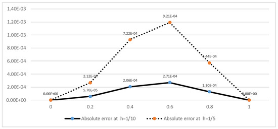
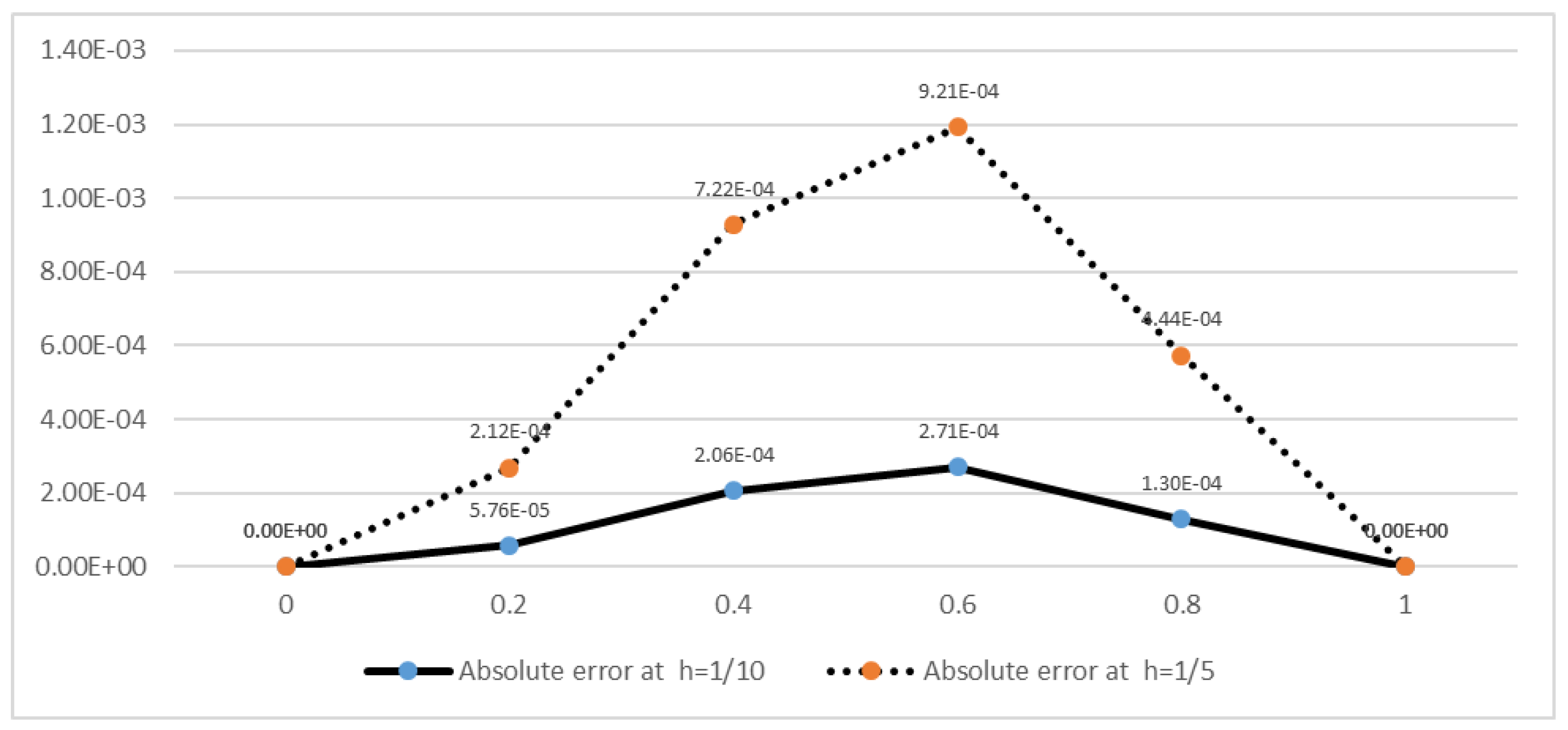
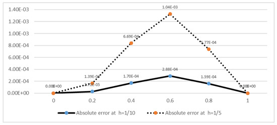
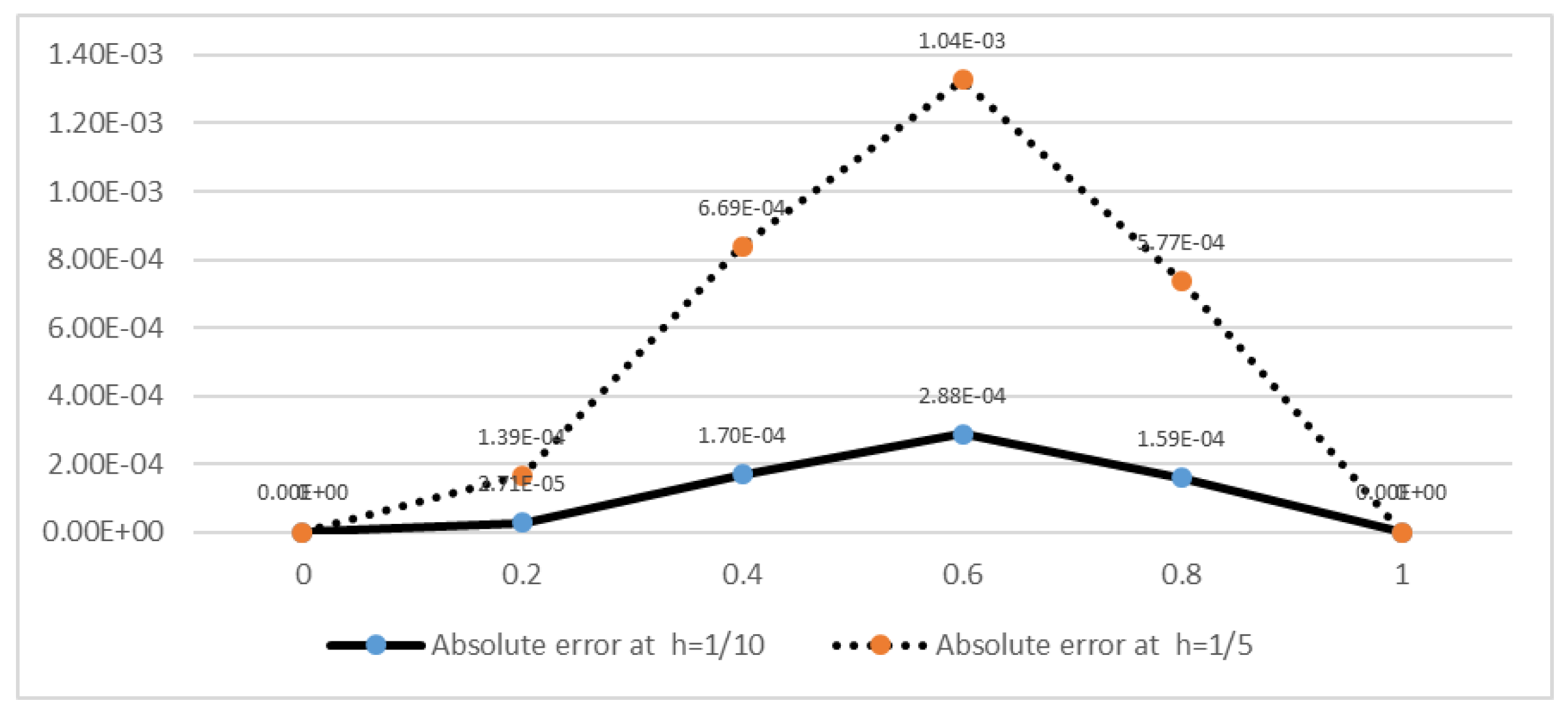
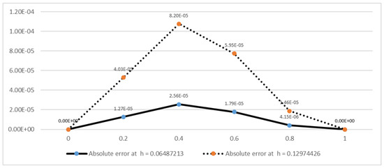
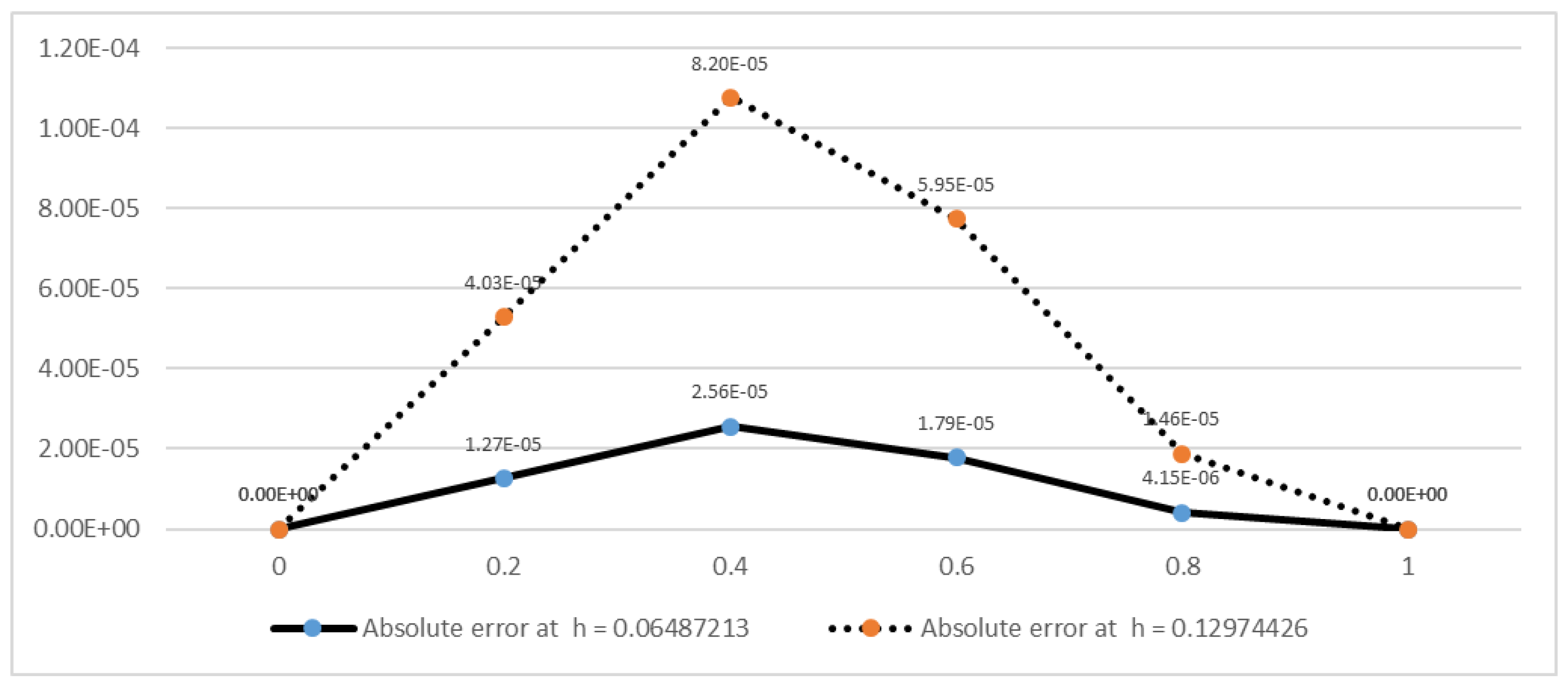
The precise solution is $w(z)=(1-z)e^z$. Arithmetical outcomes for this problem are revealed in Table 2 for $h=\frac{1}{10}$. The graphical comparison between absolute errors at $h=\frac{1}{10}$ and $h=\frac{1}{5}$ is demonstrated in Figure 1. At $h=\frac{1}{10}$ we will have unknowns ${\ell }_i$ where $(i=-2,-1,0,1,\dots ,n+2)$. At $n=10$ we will have seven equations from Equation (22), four equations from Equation (23), four equations from Equation (24), so total we will have fifteen equations and fifteen unknowns.

Table 2. Comparison of exact solution and Cubic B-spline solution of Problem 1 at $h=\frac{1}{10}$.

z	Exact Solution of	Cubic B-Spline Solution	Absolute Error of CBS	[31]
0	1	1	0	0
0.1	0.99465382626808	0.99464003039971	1.38 $\times {10}^{-5}$	5.96 $\times {10}^{-7}$
0.2	0.97712220652814	0.97706460667836	5.76 $\times {10}^{-5}$	6.56 $\times {10}^{-7}$
0.3	0.94490116530320	0.94477345208706	1.28 $\times {10}^{-4}$	1.19 $\times {10}^{-7}$
0.4	0.89509481858476	0.89488924463764	2.06 $\times {10}^{-4}$	9.54 $\times {10}^{-7}$
0.5	0.82436063535006	0.82409833674802	2.62 $\times {10}^{-4}$	2.03 $\times {10}^{-6}$
0.6	0.72884752015620	0.72857639555592	2.71 $\times {10}^{-4}$	3.70 $\times {10}^{-6}$
0.7	0.60412581224114	0.60390411609609	2.22 $\times {10}^{-4}$	5.07 $\times {10}^{-6}$
0.8	0.44510818569849	0.44497804890510	1.30 $\times {10}^{-4}$	4.29 $\times {10}^{-6}$
0.9	0.24596031111570	0.24592145969977	3.89 $\times {10}^{-5}$	2.15 $\times {10}^{-6}$
1	0	0	0	0

Figure 1. Graphical comparison of Problem 1 at $h=\frac{1}{10}$ and $h=\frac{1}{5}$.

Arithmetical outcomes for this problem are revealed in Table 3 for $h=\frac{1}{5}$. At $n=5$ we will have two equation from Equation (22), four equations from Equation (23), four equations from Equation (24), so total we will have ten equations and ten unknowns.

Table 3. Comparison of exact solution and Cubic B-spline solution of Problem 1 at $h=\frac{1}{5}$.

z	Exact Solution of	Cubic B-Spline Solution	Absolute Error of CBS
0	1	1	0
0.2	0.97712220652814	0.97691002752530	2.12 $\times {10}^{-4}$
0.4	0.89509481858476	0.89437324656962	7.22 $\times {10}^{-4}$
0.6	0.72884752015620	0.72792627066555	9.21 $\times {10}^{-4}$
0.8	0.44510818569849	0.44466410737581	4.44 $\times {10}^{-4}$
1	0	0	0

Absolute errors at all derivatives are described in Table 4.

Table 4. Absolute errors at all derivatives at $h=\frac{1}{10}$ where boundary conditions are defined in Problem 1.

z	Cubic B-Spline Solution of ${\mathit{w}}^{(1)}(\mathit{z})$	Exact Solution of ${\mathit{w}}^{(1)}(\mathit{z})$	Absolute Error of ${\mathit{w}}^{(1)}(\mathit{z})$	Exact Solution of ${\mathit{w}}^{(2)}(\mathit{z})$	Cubic B-Spline Solution of ${\mathit{w}}^{(2)}(\mathit{z})$	Absolute Error of ${\mathit{w}}^{(2)}(\mathit{z})$	Exact Solution of ${\mathit{w}}^{(3)}(\mathit{z})$	Cubic B-Spline Solution of ${\mathit{w}}^{(3)}(\mathit{z})$	Absolute Error of ${\mathit{w}}^{(3)}(\mathit{z})$
0	0	0	0	−1	−1	0	−2	−2	0
0.1	−0.1105	−0.1108	2.82 $\times {10}^{-4}$	−1.2157	−1.2160	2.94 $\times {10}^{-4}$	−2.3208	−2.3267	5.87 $\times {10}^{-3}$
0.2	−0.2443	−0.2449	5.85 $\times {10}^{-4}$	−1.4649	−1.4653	3.38 $\times {10}^{-4}$	−2.6738	−2.6805	6.62 $\times {10}^{-3}$
0.3	−0.4049	−0.4057	7.79 $\times {10}^{-4}$	−1.7493	−1.7521	2.74 $\times {10}^{-3}$	−3.0637	−3.0842	2.05 $\times {10}^{-2}$
0.4	−0.5966	−0.5974	7.20 $\times {10}^{-4}$	−2.0758	−2.0822	6.37 $\times {10}^{-3}$	−3.5308	−3.5556	2.48 $\times {10}^{-2}$
0.5	−0.8243	−0.8247	3.58 $\times {10}^{-4}$	−2.4533	−2.4632	9.88 $\times {10}^{-3}$	−4.0926	−4.1072	1.46 $\times {10}^{-2}$
0.6	−1.0928	−1.0931	2.11 $\times {10}^{-4}$	−2.8918	−2.9036	1.18 $\times {10}^{-2}$	−4.7375	−4.7464	8.87 $\times {10}^{-3}$
0.7	−1.4081	−1.4089	7.61 $\times {10}^{-4}$	−3.4016	−3.4125	1.09 $\times {10}^{-2}$	−5.4371	−5.4755	3.84 $\times {10}^{-2}$
0.8	−1.7783	−1.7794	1.01 $\times {10}^{-3}$	−3.9914	−3.9987	7.24 $\times {10}^{-3}$	−6.2315	−6.2921	6.06 $\times {10}^{-2}$
0.9	−2.2121	−2.2129	7.34 $\times {10}^{-4}$	−4.6685	−4.6709	2.34 $\times {10}^{-3}$	−7.1329	−7.1892	5.63 $\times {10}^{-2}$
1	−2.7183	−2.7183	0	−5.4365	−5.4365	0	−8.1548	−8.1548	0

7.2. Problem 2

Consider the linear 8th order BVP’s ([23,30,31,34])

$$w^{(8)}(z)+zw(z)=-e^z(48+15z+z^3),0\le z\le 1$$

subject to

$$w(0)=0,w(1)=0,w^{(1)}(0)=1,w^{(1)}(1)=-e,$$

$$w^{(2)}(0)=0,w^{(2)}(1)=-4e,w^{(3)}(0)=-3,w^{(3)}(1)=-9e.$$

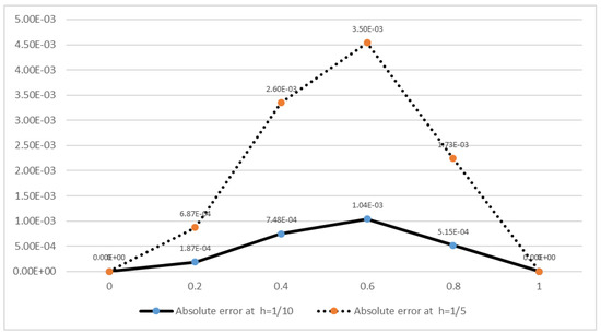
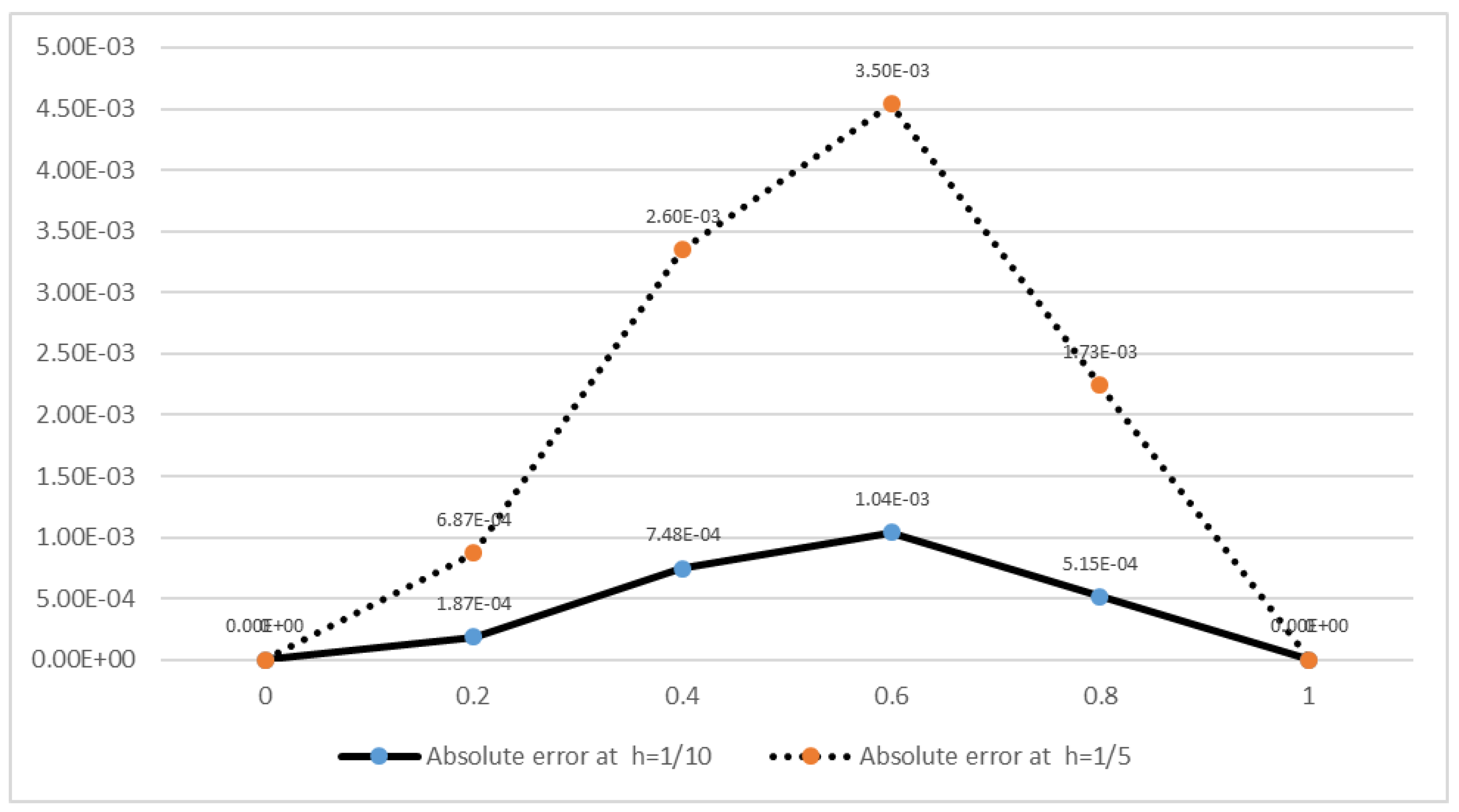
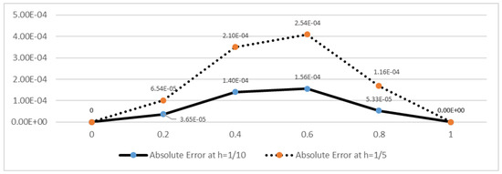
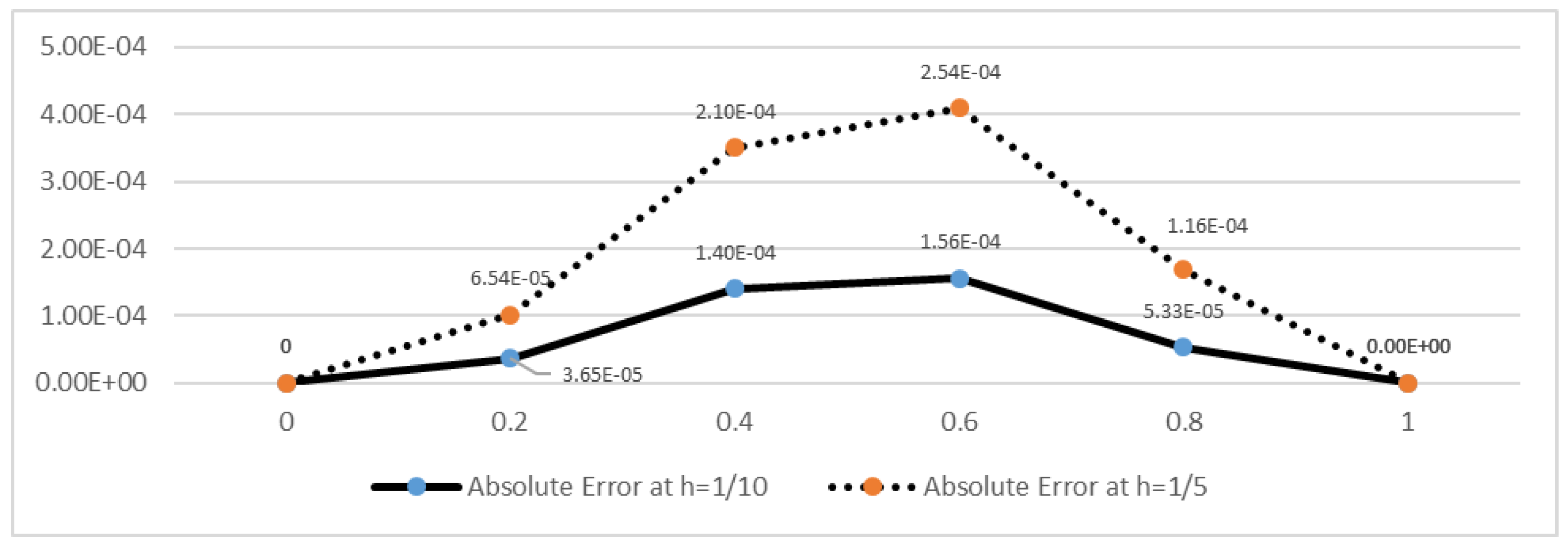
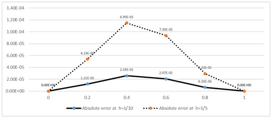
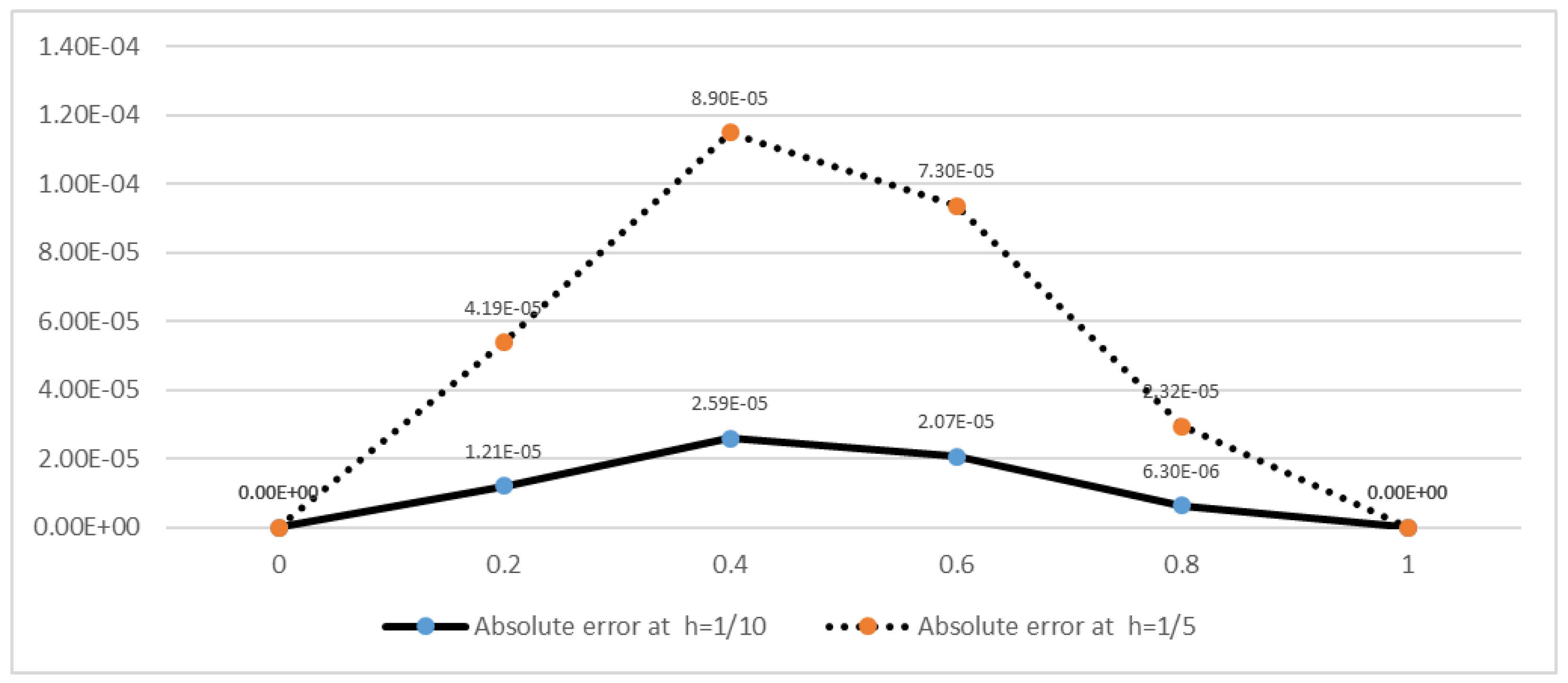
The precise solution is $w(z)=z(1-z)e^z$. Algebraic outcomes for this problem are presented in Table 5 for $h=\frac{1}{10}$. The graphical comparison between absolute errors at $h=\frac{1}{10}$ and $h=\frac{1}{5}$ is demonstrated in Figure 2. At $h=\frac{1}{10}$ we will have unknowns ${\ell }_i$$(i=-2,-1,0,1,\dots ,n+2)$ where. At $n=10$ we will have seven equations from Equation (22), four equations from Equation (23), four equations from Equation (24), so total we will have fifteen equations and fifteen unknowns.

Table 5. Comparison of exact solution and Cubic B-spline solution of Problem 2 at $h=\frac{1}{10}$.

z	Exact Solution of	Cubic B-Spline Solution	Absolute Error of CBS	[31]
0	0	0	0	0
0.1	0.09946538262681	0.09942405954487	4.13 $\times {10}^{-5}$	2.46 $\times {10}^{-7}$
0.2	0.19542444130563	0.19523703705762	1.87 $\times {10}^{-4}$	8.19 $\times {10}^{-7}$
0.3	0.28347034959096	0.28302687772238	4.43 $\times {10}^{-4}$	1.99 $\times {10}^{-6}$
0.4	0.35803792743391	0.35728987754939	7.48 $\times {10}^{-4}$	4.29 $\times {10}^{-6}$
0.5	0.41218031767503	0.41119364975850	9.87 $\times {10}^{-4}$	6.19 $\times {10}^{-6}$
0.6	0.43730851209372	0.43626438816196	1.04 $\times {10}^{-3}$	7.18 $\times {10}^{-6}$
0.7	0.42288806856880	0.42202025044259	8.68 $\times {10}^{-4}$	7.03 $\times {10}^{-6}$
0.8	0.35608654855880	0.35557187302869	5.15 $\times {10}^{-4}$	5.06 $\times {10}^{-6}$
0.9	0.22136428000413	0.22121010545131	1.54 $\times {10}^{-4}$	2.41 $\times {10}^{-6}$
1	0	0	0	0

Figure 2. Graphical comparison of Problem 2 at $h=\frac{1}{10}$ and $h=\frac{1}{5}$.

Arithmetical outcomes for this problem are revealed in Table 6 for $h=\frac{1}{5}$. At $n=5$ we will have two equation from Equation (22), four equations from Equation (23), four equations from Equation (24), so total we will have ten equations and ten unknowns.

Table 6. Comparison of exact solution and Cubic B-spline solution of Problem 2 at $h=\frac{1}{5}$.

z	Exact Solution of	Cubic B-Spline Solution	Absolute Error of CBS
0	0	0	0
0.2	0.19542444130563	0.19473719409835	6.87 $\times {10}^{-4}$
0.4	0.35803792743391	0.35543924551290	2.60 $\times {10}^{-3}$
0.6	0.43730851209372	0.43381262638307	3.50 $\times {10}^{-3}$
0.8	0.35608654855880	0.35435927825085	1.73 $\times {10}^{-3}$
1	0	0	0

Absolute errors at all derivatives are described in Table 7.

Table 7. Absolute errors at all derivatives at $h=\frac{1}{10}$ where boundary conditions are defined in Problem 2.

z	Cubic B-Spline Solution of ${\mathit{w}}^{(1)}(\mathit{z})$	Exact Solution of ${\mathit{w}}^{(1)}(\mathit{z})$	Absolute Error of ${\mathit{w}}^{(1)}(\mathit{z})$	Exact Solution of ${\mathit{w}}^{(2)}(\mathit{z})$	Cubic B-Spline Solution of ${\mathit{w}}^{(2)}(\mathit{z})$	Absolute Error of ${\mathit{w}}^{(2)}(\mathit{z})$	Exact Solution of ${\mathit{w}}^{(3)}(\mathit{z})$	Cubic B-Spline Solution of ${\mathit{w}}^{(3)}(\mathit{z})$	Absolute Error of ${\mathit{w}}^{(3)}(\mathit{z})$
0	1	1	0	0	0	0	−3	−3	0
0.1	0.9836	0.9827	8.80 $\times {10}^{-4}$	−0.3426	−0.3456	2.96 $\times {10}^{-3}$	−3.8792	−3.922	4.28 $\times {10}^{-2}$
0.2	0.9282	0.9262	2.04 $\times {10}^{-3}$	−0.7817	−0.7844	2.69 $\times {10}^{-3}$	−4.9174	−4.9259	8.54 $\times {10}^{-3}$
0.3	0.8235	0.8205	2.95 $\times {10}^{-3}$	−1.3251	−1.3307	5.61 $\times {10}^{-3}$	−6.0474	−6.1216	7.42 $\times {10}^{-2}$
0.4	0.6564	0.6535	2.91 $\times {10}^{-3}$	−1.9885	−2.0087	2.02 $\times {10}^{-2}$	−7.4939	−7.5959	1.02 $\times {10}^{-1}$
0.5	0.4122	0.4106	1.62 $\times {10}^{-3}$	−2.8146	−2.8499	3.53 $\times {10}^{-2}$	−9.3467	−9.4134	6.67 $\times {10}^{-2}$
0.6	0.0741	0.0735	6.11 $\times {10}^{-4}$	−3.8470	−3.8914	4.44 $\times {10}^{-2}$	−11.5887	−11.6174	2.87 $\times {10}^{-2}$
0.7	−0.3768	−0.3797	2.87 $\times {10}^{-3}$	−5.1312	−5.1734	4.22 $\times {10}^{-2}$	−14.0766	−14.2306	1.54 $\times {10}^{-1}$
0.8	−0.9714	−0.9753	3.95 $\times {10}^{-3}$	−6.7094	−6.7375	2.81 $\times {10}^{-2}$	−17.0029	−17.2559	2.53 $\times {10}^{-1}$
0.9	−1.7405	−1.7434	2.92 $\times {10}^{-3}$	−8.6160	−8.6246	8.62 $\times {10}^{-3}$	−20.4391	−20.6781	2.39 $\times {10}^{-1}$
1	−2.7183	−2.7183	0	−10.8731	−10.8731	0	−24.4645	−24.4645	0

7.3. Problem 3

Consider the linear 8th order BVP’s ([23,30,31])

$$w^{(8)}(z)-w(z)=-8(2zcos(z)+7sin(z)),0\le z\le 1$$

subject to

$$w(0)=0,w(1)=0,w^{(1)}(0)=-1,w^{(1)}(1)=2sin(1),$$

$$w^{(2)}(0)=0,w^{(2)}(1)=4cos(1)+2sin(1),$$

$$w^{(3)}(0)=7,w^{(3)}(1)=-6sin(1)+6cos(1).$$

The exact solution is $w(z)=({(z)}^2-1)sin(z)$. Arithmetical outcomes for this problem are revealed in Table 8 for $h=\frac{1}{10}$. The graphical comparison between absolute errors at $h=\frac{1}{10}$ and $h=\frac{1}{5}$ is demonstrated in Figure 3. At $h=\frac{1}{10}$ we will have unknowns ${\ell }_i$ $(i=-2,-1,0,1,\dots ,n+2)$ where. At $n=10$ we will have seven equations from Equation (22), four equations from Equation (23), four equations from Equation (24), so total we will have fifteen equations and fifteen unknowns.

Table 8. Comparison of exact solution and Cubic B-spline solution of Problem 3 at $h=\frac{1}{10}$.

z	Exact Solution of	Cubic B-Spline Solution	Absolute Error of CBS	[23]
0	0	0	0	0
0.1	−0.09883508248036	−0.09883929795528	4.22 $\times {10}^{-6}$	3.97 $\times {10}^{-7}$
0.2	−0.19072255756326	−0.19074966511972	2.71 $\times {10}^{-5}$	9.32 $\times {10}^{-7}$
0.3	−0.26892338806182	−0.26900781261417	8.44 $\times {10}^{-5}$	6.78 $\times {10}^{-6}$
0.4	−0.32711140753927	−0.32728094968339	1.70 $\times {10}^{-4}$	1.08 $\times {10}^{-5}$
0.5	−0.35956915395315	−0.35982014743648	2.51 $\times {10}^{-4}$	1.83 $\times {10}^{-4}$
0.6	−0.36137118297282	−0.36165941441105	2.88 $\times {10}^{-4}$	3.21 $\times {10}^{-4}$
0.7	−0.32855102049122	−0.32880597250785	2.55 $\times {10}^{-4}$	6.73 $\times {10}^{-3}$
0.8	−0.25824819272383	−0.25840750142588	1.59 $\times {10}^{-4}$	1.27 $\times {10}^{-3}$
0.9	−0.14883211282922	−0.14888246114063	5.03 $\times {10}^{-5}$	2.47 $\times {10}^{-3}$
1	0	0	0	0

Figure 3. Graphical comparison of Problem 3 at $h=\frac{1}{10}$ and $h=\frac{1}{5}$.

Arithmetical outcomes for this problem are revealed in Table 9 for $h=\frac{1}{5}$. At $n=5$ we will have two equation from Equation (22), four equations from Equation (23), four equations from Equation (24), so total we will have ten equations and ten unknowns.

Table 9. Comparison of exact solution and Cubic B-spline solution of Problem 3 at $h=\frac{1}{5}$.

z	Exact Solution of	Cubic B-Spline Solution	Absolute Error of CBS
0	0	0	0
0.2	−0.19072255756326	−0.19086203871595	1.39 $\times {10}^{-4}$
0.4	−0.32711140753927	−0.32778034786133	6.69 $\times {10}^{-4}$
0.6	−0.36137118297282	−0.36241298481970	1.04 $\times {10}^{-3}$
0.8	−0.25824819272383	−0.25882550188894	5.77 $\times {10}^{-4}$
1	0	0	0

Absolute errors at all derivatives are described in Table 10.

Table 10. Absolute errors at all derivatives at $h=\frac{1}{10}$ where boundary conditions are defined in Problem 3.

z	Cubic B-Spline Solution of ${\mathit{w}}^{(1)}(\mathit{z})$	Exact Solution of ${\mathit{w}}^{(1)}(\mathit{z})$	Absolute Error of ${\mathit{w}}^{(1)}(\mathit{z})$	Exact Solution of ${\mathit{w}}^{(2)}(\mathit{z})$	Cubic B-Spline Solution of ${\mathit{w}}^{(2)}(\mathit{z})$	Absolute Error of ${\mathit{w}}^{(2)}(\mathit{z})$	Exact Solution of ${\mathit{w}}^{(3)}(\mathit{z})$	Cubic B-Spline Solution of ${\mathit{w}}^{(3)}(\mathit{z})$	Absolute Error of ${\mathit{w}}^{(3)}(\mathit{z})$
0	−1	−1	0	0	0	0	7	7	0
0.1	−0.9651	−0.9652	9.15 $\times {10}^{-5}$	0.6965	0.6964	8.24 $\times {10}^{-5}$	6.8952	6.8584	3.68 $\times {10}^{-2}$
0.2	−0.8614	−0.8618	3.78 $\times {10}^{-4}$	1.3721	1.3717	4.41 $\times {10}^{-4}$	6.5829	6.559	2.39 $\times {10}^{-2}$
0.3	−0.6921	−0.6928	7.36 $\times {10}^{-4}$	2.0101	2.0082	1.85 $\times {10}^{-3}$	6.0785	6.074	4.53 $\times {10}^{-3}$
0.4	−0.4621	−0.463	8.89 $\times {10}^{-4}$	2.5933	2.5865	6.82 $\times {10}^{-3}$	5.4152	5.3903	2.49 $\times {10}^{-2}$
0.5	−0.1788	−0.1794	6.47 $\times {10}^{-4}$	3.0990	3.0863	1.27 $\times {10}^{-2}$	4.5338	4.5096	2.42 $\times {10}^{-2}$
0.6	0.1493	0.1493	3.15 $\times {10}^{-5}$	3.5053	3.4884	1.69 $\times {10}^{-2}$	3.4479	3.4477	2.11 $\times {10}^{-4}$
0.7	0.5132	0.5125	7.00 $\times {10}^{-4}$	3.7931	3.7758	1.73 $\times {10}^{-2}$	2.2734	2.2348	3.86 $\times {10}^{-2}$
0.8	0.8992	0.8981	1.14 $\times {10}^{-3}$	3.9482	3.9353	1.29 $\times {10}^{-2}$	0.9878	0.9146	7.32 $\times {10}^{-2}$
0.9	1.2937	1.2928	9.15 $\times {10}^{-4}$	3.9642	3.9587	5.46 $\times {10}^{-3}$	−0.3822	−0.456	7.38 $\times {10}^{-2}$
1	1.6829	1.6829	0	3.8442	3.8442	0	−1.8070	−1.8070	0

7.4. Problem 4

$$w{}^{(8)}(z)+w{}^{(3)}(z)sin(w(z))=e^z(1+sin(e^z)),0\le z\le 1$$

Subject to

$$w(0)=1,w(1)=e,$$

$$w{}^{(1)}(0)=1,w{}^{(1)}(1)=e$$

$$w{}^{(2)}(0)=1,w{}^{(2)}(1)=e,$$

$$w{}^{(3)}(0)=1,w{}^{(3)}(1)=e.$$

The exact solution for the above problem is given by $w(z)=e^z$. Arithmetical outcomes for this problem are presented in Table 11 for $h=\frac{1}{10}$. The graphical comparison between absolute errors at $h=\frac{1}{10}$ and $h=\frac{1}{5}$ is presented in Figure 4. At $h=\frac{1}{10}$ or $n=10$, there will be unknown values $l{}_i$ where $(i=-2,-1,0,1,\cdots ,n+2)$ so, there will be seven equations from Equation (22), four equations from Equation (23), four equations from Equation (26), so totally, there will be fifteen equations and fifteen unknown values.

Table 11. Comparison of exact solution and presented method solution of Problem 4 at $h=\frac{1}{10}$.

z	Exact Solution	Presented Method Solution	Absolute Error	[30]
0	1	1	0	0
0.1	1.10517091807564	1.10517794712470	7.03 $\times {10}^{-6}$	2.50 $\times {10}^{-6}$
0.2	1.22140275816017	1.22143922353981	3.65 $\times {10}^{-5}$	8.94 $\times {10}^{-6}$
0.3	1.34985880757600	1.34994628964200	8.75 $\times {10}^{-5}$	1.56 $\times {10}^{-5}$
0.4	1.49182469764127	1.49196477025922	1.40 $\times {10}^{-4}$	1.82 $\times {10}^{-5}$
0.5	1.64872127070012	1.64888916217970	1.68 $\times {10}^{-4}$	8.82 $\times {10}^{-6}$
0.6	1.82211880039050	1.82227459457679	1.56 $\times {10}^{-4}$	7.51 $\times {10}^{-6}$
0.7	2.01375270747047	2.01386242544904	1.10 $\times {10}^{-4}$	1.88 $\times {10}^{-5}$
0.8	2.22554092849246	2.22559418213629	5.33 $\times {10}^{-5}$	1.93 $\times {10}^{-5}$
0.9	2.45960311115695	2.45961577150042	1.27 $\times {10}^{-5}$	1.16 $\times {10}^{-5}$
1	2.71828182845905	2.71828182845905	0	0

Figure 4. Graphical comparison of Problem 4 at $h=\frac{1}{10}$ and $h=\frac{1}{5}$.

Arithmetical outcomes for this problem are presented in Table 12 for $h=\frac{1}{5}$ or $n=5$, there will be two equation from Equation (22), four equations from Equation (23), four equations from Equation (26), so totally, there will be ten equations and ten unknown values.

Table 12. Comparison of exact solution and presented method solution of Problem 4 at $h=\frac{1}{5}$.

z	Exact Solution	Presented Method Solution	Absolute Error
0	1	1	0
0.2	1.22140275816017	1.22146817204786	6.54 $\times {10}^{-5}$
0.4	1.49182469764127	1.49203484074618	2.10 $\times {10}^{-4}$
0.6	1.82211880039050	1.82237276345783	2.54 $\times {10}^{-4}$
0.8	2.22554092849246	2.22565718003072	1.16 $\times {10}^{-4}$
1	2.71828182845905	2.71828182845905	0

Absolute errors at all derivatives are described in Table 13.

Table 13. Absolute errors at all derivatives at $h=\frac{1}{10}$ where boundary conditions are defined in Problem 4.

z	Cubic B-Spline Solution of ${\mathit{w}}^{(1)}(\mathit{z})$	Exact Solution of ${\mathit{w}}^{(1)}(\mathit{z})$	Absolute Error of ${\mathit{w}}^{(1)}(\mathit{z})$	Exact Solution of ${\mathit{w}}^{(2)}(\mathit{z})$	Cubic B-Spline Solution of ${\mathit{w}}^{(2)}(\mathit{z})$	Absolute Error of ${\mathit{w}}^{(2)}(\mathit{z})$	Exact Solution of ${\mathit{w}}^{(3)}(\mathit{z})$	Cubic B-Spline Solution of ${\mathit{w}}^{(3)}(\mathit{z})$	Absolute Error of ${\mathit{w}}^{(3)}(\mathit{z})$
0	1	1	0	1	1	0	1	1	0
0.1	1.1055	1.10534	1.67 $\times {10}^{-4}$	1.1084	1.10677	1.60 $\times {10}^{-3}$	1.1241	1.11462	9.45 $\times {10}^{-3}$
0.2	1.2222	1.22182	4.20 $\times {10}^{-4}$	1.2244	1.22292	1.52 $\times {10}^{-3}$	1.2214	1.2112	1.02 $\times {10}^{-2}$
0.3	1.3510	1.35042	5.61 $\times {10}^{-4}$	1.3499	1.34901	8.51 $\times {10}^{-4}$	1.3499	1.32485	2.50 $\times {10}^{-2}$
0.4	1.4927	1.49226	4.40 $\times {10}^{-4}$	1.4918	1.48789	3.93 $\times {10}^{-3}$	1.4918	1.46978	2.20 $\times {10}^{-2}$
0.5	1.6489	1.64881	8.64 $\times {10}^{-5}$	1.6487	1.64296	5.76 $\times {10}^{-3}$	1.6487	1.6449	3.82 $\times {10}^{-3}$
0.6	1.8221	1.8218	3.19 $\times {10}^{-4}$	1.8221	1.81687	5.25 $\times {10}^{-3}$	1.8581	1.84009	1.80 $\times {10}^{-2}$
0.7	2.0138	2.01319	5.60 $\times {10}^{-4}$	2.0138	2.01098	2.77 $\times {10}^{-3}$	2.0730	2.04339	2.96 $\times {10}^{-2}$
0.8	2.2255	2.22502	5.22 $\times {10}^{-4}$	2.2256	2.22555	1.03 $\times {10}^{-5}$	2.2718	2.24865	2.31 $\times {10}^{-2}$
0.9	2.4596	2.45933	2.71 $\times {10}^{-4}$	2.4618	2.46071	1.11 $\times {10}^{-3}$	2.4677	2.46365	4.05 $\times {10}^{-3}$
1	2.7182	2.7182	0	2.7182	2.7182	0	2.7182	2.7182	0

7.5. Problem 5

$$w{}^{(8)}(z)=7!(e{}^{-}{}^{8w(z)}-\frac{2}{{\left(1+z\right)}^8}),0\le z\le e^{\frac{1}{2}}-1$$

subject to

$$w(0)=0,w(e^{\frac{1}{2}}-1)=\frac{1}{2},$$

$$w{}^{(1)}(0)=1,w{}^{(1)}(e^{\frac{1}{2}}-1)=e^{-\frac{1}{2}},$$

$$w{}^{(2)}(0)=-1,w{}^{(2)}(e^{\frac{1}{2}}-1)=-e^{-1},$$

$$w{}^{(3)}(0)=2,w{}^{(3)}(e^{\frac{1}{2}}-1)={2e}^{-\frac{3}{2}}.$$

The precise solution for the overhead problem is specified by $w(z)=ln(1+z)$. The suggested technique is confirmed on this problem where the domain [0, $e^{\frac{1}{2}}-1$] for $h={2^{-i}(e}^{\frac{1}{2}}-1).$ Algebraic outcomes for this problem are presented in Table 14 for $h=0.06487213$. The graphical comparison between absolute errors at $h=0.06487213$ and $h=0.12974426$ is presented in Figure 5. At $h=0.06487213$ and $n=10$, there will be unknown values $l{}_i$ where $(i=-2,-1,0,1,\cdots ,n+2)$ so, there will be seven equations from Equation (22), four equations from Equation (23), four equations from Equation (26), so totally, there will be fifteen equations and fifteen unknown values.

Table 14. Comparison of exact solution and presented method solution of Problem 5 at $h=0.06487213$.

z	Exact Solution	Presented Method Solution	Absolute Error	[30]	[34]	[36]	[37]
0	0	0	0	0	0	0	0
0.064	0.0628547262	0.0628509884	3.74 $\times {10}^{-6}$	3.42 $\times {10}^{-7}$	1.42 $\times {10}^{-7}$	2.01 $\times {10}^{-7}$	2.94 $\times {10}^{-6}$
0.129	0.1219912885	0.1219786318	1.27 $\times {10}^{-5}$	4.10 $\times {10}^{-7}$	1.07 $\times {10}^{-6}$	4.54 $\times {10}^{-7}$	1.58 $\times {10}^{-5}$
0.194	0.1778251212	0.1778037262	2.14 $\times {10}^{-5}$	2.68 $\times {10}^{-7}$	3.37 $\times {10}^{-6}$	1.52 $\times {10}^{-6}$	2.91 $\times {10}^{-5}$
0.259	0.2307057020	0.2306800632	2.56 $\times {10}^{-5}$	1.42 $\times {10}^{-6}$	7.02 $\times {10}^{-6}$	4.07 $\times {10}^{-6}$	4.91 $\times {10}^{-5}$
0.324	0.2809298146	0.2809058296	2.40 $\times {10}^{-5}$	3.34 $\times {10}^{-6}$	9.54 $\times {10}^{-6}$	6.71 $\times {10}^{-6}$	7.34 $\times {10}^{-5}$
0.389	0.3287516379	0.3287337725	1.79 $\times {10}^{-5}$	5.84 $\times {10}^{-6}$	1.07 $\times {10}^{-5}$	9.06 $\times {10}^{-6}$	8.51 $\times {10}^{-5}$
0.454	0.3743905291	0.3743802408	1.03 $\times {10}^{-5}$	7.90 $\times {10}^{-6}$	1.03 $\times {10}^{-5}$	1.00 $\times {10}^{-5}$	6.54 $\times {10}^{-5}$
0.518	0.4180371082	0.4180329583	4.15 $\times {10}^{-6}$	4.80 $\times {10}^{-6}$	5.22 $\times {10}^{-6}$	5.45 $\times {10}^{-6}$	4.38 $\times {10}^{-5}$
0.583	0.4598580678	0.4598572086	8.59 $\times {10}^{-7}$	2.41 $\times {10}^{-6}$	2.41 $\times {10}^{-6}$	2.59 $\times {10}^{-6}$	2.31 $\times {10}^{-5}$
0.648	0.5	0.5	0	0	0	0	0

Figure 5. Graphical comparison of Problem 5 at $h=0.06487213$ and $h=0.12974426$.

Arithmetical outcomes for this problem are presented in Table 15 for $h=0.12974426$ and $n=5$, there will be two equation from Equation (22), four equations from Equation (23), four equations from Equation (26), so totally, there will be ten equations and ten unknown values.

Table 15. Comparison of exact solution and presented method solution of Problem 5 at $h=0.12974426$.

z	Exact Solution	Presented Method Solution	Absolute Error
0	0	0	0
0.129	0.12199128852626	0.12195103139582	4.03 $\times {10}^{-5}$
0.259	0.23070570204092	0.23062366023811	8.20 $\times {10}^{-5}$
0.389	0.32875163792382	0.32869211718688	5.95 $\times {10}^{-5}$
0.518	0.41803710829203	0.41802254868918	1.46 $\times {10}^{-5}$
0.648	0.5	0.5	0

Absolute errors at all derivatives are described in Table 16.

Table 16. Absolute errors at all derivatives at $h=\frac{1}{10}$ where boundary conditions are defined in Problem 5.

z	Cubic B-Spline Solution of ${\mathit{w}}^{(1)}(\mathit{z})$	Exact Solution of ${\mathit{w}}^{(1)}(\mathit{z})$	Absolute Error of ${\mathit{w}}^{(1)}(\mathit{z})$	Exact Solution of ${\mathit{w}}^{(2)}(\mathit{z})$	Cubic B-Spline Solution of ${\mathit{w}}^{(2)}(\mathit{z})$	Absolute Error of ${\mathit{w}}^{(2)}(\mathit{z})$	Exact Solution of ${\mathit{w}}^{(3)}(\mathit{z})$	Cubic B-Spline Solution of ${\mathit{w}}^{(3)}(\mathit{z})$	Absolute Error of ${\mathit{w}}^{(3)}(\mathit{z})$
0	0	0	0	0	0	0	0	0	0
0.064	0.9399	0.93897	8.81 $\times {10}^{-4}$	−0.8799	−0.8816	1.73 $\times {10}^{-3}$	1.6984	1.67938	1.90 $\times {10}^{-2}$
0.129	0.8857	0.885	7.35 $\times {10}^{-4}$	−0.7797	−0.7821	2.42 $\times {10}^{-3}$	1.4326	1.41121	2.14 $\times {10}^{-2}$
0.194	0.8375	0.83698	5.41 $\times {10}^{-4}$	−0.6955	−0.6985	2.95 $\times {10}^{-3}$	1.2001	1.18751	1.26 $\times {10}^{-2}$
0.259	0.7943	0.79395	3.28 $\times {10}^{-4}$	−0.6252	−0.628	2.85 $\times {10}^{-3}$	1.0041	1.00314	9.46 $\times {10}^{-4}$
0.324	0.7553	0.75515	1.40 $\times {10}^{-4}$	−0.5662	−0.5683	2.12 $\times {10}^{-3}$	0.8617	0.85397	7.75 $\times {10}^{-3}$
0.389	0.7199	0.71994	7.23 $\times {10}^{-6}$	−0.5162	−0.5172	1.08 $\times {10}^{-3}$	0.7463	0.73574	1.06 $\times {10}^{-2}$
0.454	0.6879	0.68782	6.17 $\times {10}^{-5}$	−0.4727	−0.4729	1.31 $\times {10}^{-4}$	0.6506	0.64331	7.33 $\times {10}^{-3}$
0.518	0.6588	0.65841	3.50 $\times {10}^{-4}$	−0.4336	−0.4338	1.93 $\times {10}^{-4}$	0.5718	0.57012	1.64 $\times {10}^{-3}$
0.583	0.6317	0.6314	3.10 $\times {10}^{-4}$	−0.3988	−0.3989	1.50 $\times {10}^{-4}$	0.5116	0.50788	3.70 $\times {10}^{-3}$
0.648	0.6065	0.6065	0	−0.3678	−0.3678	0	0.4462	0.4462	0

7.6. Problem 6

$$w{}^{(8)}(z)+e^{-}{}^z(w(z)){}^2=e^{-}{}^z+e^{-3z},0\le z\le 1$$

subject to

$$w(0)=1,w(1)=e^{-1},$$

$$w{}^{(1)}(0)=-1,w{}^{(1)}(1)=-e^{-1},$$

$$w{}^{(2)}(0)=1,w{}^{(2)}(1)=e^{-1},$$

$$w{}^{(3)}(0)=-1,w{}^{(3)}(1)=-e^{-1}.$$

The exact solution for the above problem is given by $w(z)=e^{-z}$. Arithmetical outcomes for this problem are presented in Table 17 for $h=\frac{1}{10}$. The graphical comparison between absolute errors at $h=\frac{1}{10}$ and $h=\frac{1}{5}$ is presented in Figure 6. At $h=\frac{1}{10}$ or $n=10$, there will be unknowns $l{}_i$ where $(i=-2,-1,0,1,\cdots ,n+2)$ so, there will be seven equations from Equation (22), four equations from Equation (23), four equations from Equation (26), so totally, there will be fifteen equations and fifteen unknowns.

Table 17. Comparison of exact solution and presented method solution of Problem 6 at $h=\frac{1}{10}$.

z	Exact Solution	Presented Method Solution	Absolute Error	[30]	[36]
0	1	1	0	0	0
0.1	0.90483741803596	0.90484101917459	3.60 $\times {10}^{-6}$	6.56 $\times {10}^{-7}$	3.58 $\times {10}^{-7}$
0.2	0.81873075307798	0.81874287120508	1.21 $\times {10}^{-5}$	9.54 $\times {10}^{-6}$	6.32 $\times {10}^{-6}$
0.3	0.74081822068172	0.74083908532179	2.09 $\times {10}^{-5}$	4.11 $\times {10}^{-6}$	1.90 $\times {10}^{-5}$
0.4	0.67032004603564	0.67034596914992	2.59 $\times {10}^{-5}$	6.74 $\times {10}^{-6}$	3.10 $\times {10}^{-5}$
0.5	0.60653065971263	0.60655628570162	2.56 $\times {10}^{-5}$	8.76 $\times {10}^{-6}$	3.64 $\times {10}^{-5}$
0.6	0.54881163609403	0.54883230312747	2.07 $\times {10}^{-5}$	8.40 $\times {10}^{-6}$	3.17 $\times {10}^{-5}$
0.7	0.49658530379141	0.49659863075283	1.33 $\times {10}^{-5}$	5.84 $\times {10}^{-6}$	1.93 $\times {10}^{-5}$
0.8	0.44932896411722	0.44933526163887	6.30 $\times {10}^{-6}$	2.95 $\times {10}^{-6}$	7.18 $\times {10}^{-6}$
0.9	0.40656965974060	0.40657124798308	1.59 $\times {10}^{-6}$	1.22 $\times {10}^{-6}$	1.46 $\times {10}^{-6}$
1	0.36787944117144	0.36787944117144	0	0	0

Figure 6. Graphical comparison of Problem 6 at $h=\frac{1}{10}$ and $h=\frac{1}{5}$.

Arithmetical outcomes for this problem are presented in Table 18 for $h=\frac{1}{5}$ or $n=5$, there will be two equation from Equation (22), four equations from Equation (23), four equations from Equation (26), so totally, there will be ten equations and ten unknown values.

Table 18. Comparison of exact solution and presented method solution of Problem 6 at $h=\frac{1}{5}$.

${\mathit{z}}^{\prime }$	Exact Solution	Presented Method Solution	Absolute Error
0	1	1	0
0.2	0.81873075307798	0.81877264048934	4.19 $\times {10}^{-5}$
0.4	0.67032004603564	0.67040909568859	8.90 $\times {10}^{-5}$
0.6	0.54881163609403	0.54888461796220	7.30 $\times {10}^{-5}$
0.8	0.44932896411722	0.44935216696161	2.32 $\times {10}^{-5}$
1	0.36787944117144	0.36787944117144	0

Absolute errors at all derivatives are described in Table 19.

Table 19. Absolute errors at all derivatives at $h=\frac{1}{10}$ where boundary conditions are defined in Problem 6.

z	Cubic B-Spline Solution of ${\mathit{w}}^{(1)}(\mathit{z})$	Exact Solution of ${\mathit{w}}^{(1)}(\mathit{z})$	Absolute Error of ${\mathit{w}}^{(1)}(\mathit{z})$	Exact Solution of ${\mathit{w}}^{(2)}(\mathit{z})$	Cubic B-Spline Solution of ${\mathit{w}}^{(2)}(\mathit{z})$	Absolute error of ${\mathit{w}}^{(2)}(\mathit{z})$	Exact Solution of ${\mathit{w}}^{(3)}(\mathit{z})$	Cubic B-Spline Solution of ${\mathit{w}}^{(3)}(\mathit{z})$	Absolute Error of ${\mathit{w}}^{(3)}(\mathit{z})$
0	1	1	0	1	1	0	1	1	0
0.1	−0.9047	−0.90477	6.80 $\times {10}^{-5}$	0.9048	0.90461	2.26 $\times {10}^{-4}$	−0.9048	−0.90973	4.89 $\times {10}^{-3}$
0.2	−0.8185	−0.81864	9.46 $\times {10}^{-5}$	0.8187	0.81805	6.77 $\times {10}^{-4}$	−0.8187	−0.8241	5.37 $\times {10}^{-3}$
0.3	−0.7407	−0.74074	7.43 $\times {10}^{-5}$	0.7408	0.73979	1.03 $\times {10}^{-3}$	−0.7408	−0.74435	3.53 $\times {10}^{-3}$
0.4	−0.6703	−0.6703	2.49 $\times {10}^{-5}$	0.6703	0.66918	1.14 $\times {10}^{-3}$	−0.6703	−0.6713	9.77 $\times {10}^{-4}$
0.5	−0.6065	−0.60656	2.87 $\times {10}^{-5}$	0.6065	0.60553	9.99 $\times {10}^{-4}$	−0.6042	−0.60537	1.16 $\times {10}^{-3}$
0.6	−0.5488	−0.54888	6.57 $\times {10}^{-5}$	0.5488	0.54811	7.02 $\times {10}^{-4}$	−0.5444	−0.54658	2.23 $\times {10}^{-3}$
0.7	−0.4966	−0.49666	7.57 $\times {10}^{-5}$	0.4966	0.49622	3.70 $\times {10}^{-4}$	−0.4924	−0.4945	2.09 $\times {10}^{-3}$
0.8	−0.4493	−0.44939	6.08 $\times {10}^{-5}$	0.4493	0.44921	1.19 $\times {10}^{-4}$	−0.4472	−0.44828	1.04 $\times {10}^{-3}$
0.9	−0.4066	−0.4066	3.17 $\times {10}^{-5}$	0.4066	0.40656	1.09 $\times {10}^{-5}$	−0.4066	−0.40665	8.18 $\times {10}^{-5}$
1	−0.3678	−0.3678	0	0.3678	0.3678	0	−0.3678	−0.3678	0

8. Conclusions

A new method with Cubic B-splines as basis functions is presented to solve 8th order linear and non-linear BVP’s. The above sections prove that the cubic-B spline technique is a sensible approach for the numerical solution of the 8th order linear and non-linear BVP. The proposed method is applied to solve six problems to study the efficiency of the method. The numerical results found by this method are very close to the exact solutions. We recommend that Cubic-B spline method can also be helpful when we consider further higher order BVP’s.

References

- Agarwal, R.P. Boundary Value Problems from Higher Order Differential Equations; World Scientific: Singapore, 1986. [Google Scholar]
- Akram, G.; Rehman, H.U. Numerical solution of 8th order boundary value problems in reproducing Kernel space. Numer. Algorithms 2013, 62, 527–540. [Google Scholar] [CrossRef] [Scilit]
- Akram, G.; Siddiqi, S.S. Nonic spline solutions of 8th order boundary value problems. Appl. Math. Comput. 2006, 182, 829–845. [Google Scholar]
- Bishop, R.; Cannon, S.; Miao, S. On coupled bending and torsional vibration of uniform beams. J. Sound Vib. 1989, 131, 457–464. [Google Scholar] [CrossRef] [Scilit]
- Boutayeb, A.; Twizell, E. Finite-difference methods for the solution of special 8th-order boundary-value problems. Int. J. Comput. Math. 1993, 48, 63–75. [Google Scholar] [CrossRef] [Scilit]
- Caglar, H.; Caglar, N.; Elfaituri, K. B-spline interpolation compared with finite difference, finite element and finite volume methods which applied to two-point boundary value problems. Appl. Math. Comput. 2006, 175, 72–79. [Google Scholar] [CrossRef] [Scilit]
- Chandrasekhar, S. Hydrodynamic and Hydromagnetic Stability; Courier Corporation: New York, NY, USA, 2013. [Google Scholar]
- De Boor, C. On the convergence of odd-degree spline interpolation. J. Approx. Theory 1968, 1, 452–463. [Google Scholar] [CrossRef] [Scilit]
- Dehghan, M.; Lakestani, M. Numerical solution of nonlinear system of second-order boundary value problems using cubic B-spline scaling functions. Int. J. Comput. Math. 2008, 85, 1455–1461. [Google Scholar] [CrossRef] [Scilit]
- Davies, A.; Karageorghis, A.; Phillips, T. Spectral Galerkin methods for the primary 2-point boundary value problem in modelling viscoelastic flows. Int. J. Numer. Methods Eng. 1988, 26, 647–662. [Google Scholar] [CrossRef] [Scilit]
- Djidjeli, K.; Twizell, E.; Boutayeb, A. Numerical methods for special nonlinear boundary-value problems of order 2m. J. Comput. Appl. Math. 1993, 47, 35–45. [Google Scholar]
- Elahi, Z.; Akram, G.; Siddiqi, S.S. Numerical solution for solving special 8th-order linear boundary value problems using Legendre Galerkin method. Math. Sci. 2016, 10, 201–209. [Google Scholar] [CrossRef] [Scilit]
- Gupta, Y.; Kumar, M. B-spline method for solution of linear fourth order boundary value problem. System 2011, 1, 4. [Google Scholar]
- Prenter, P.M. Splines and Variational Methods; Courier Corporation: New York, NY, USA, 2008. [Google Scholar]
- Hall, C. On error bounds for spline interpolation. J. Approx. Theory 1968, 1, 209–218. [Google Scholar] [CrossRef] [Scilit]
- Golbabai, A.; Javidi, M. Application of homotopy perturbation method for solving 8th-order boundary value problems. Appl. Math. Comput. 2007, 191, 334–346. [Google Scholar]
- Haq, S.; Idrees, M.; Islam, S. Application of optimal Homotopy asymptotic method to 8th order initial and boundary value problems. Int. J. Appl. Math. Comput. 2010, 2, 73–80. [Google Scholar]
- He, J.-H. A coupling method of a homotopy technique and a perturbation technique for non-linear problems. Int. J. Non-Linear Mech. 2000, 35, 37–43. [Google Scholar] [CrossRef] [Scilit]
- Inç, M.; Evans, D.J. An efficient approach to approximate solutions of 8th-order boundary-value problems. Int. J. Comput. Math. 2004, 81, 685–692. [Google Scholar] [CrossRef] [Scilit]
- Khalid, A.; Naeem, M.N. Cubic B-spline Solution of Nonlinear Sixth Order Boundary Value Problems. J. Math. 2018, 50, 91–103. [Google Scholar]
- Lang, F.-G.; Xu, X.-P. A new cubic B-spline method for linear fifth order boundary value problems. J. Appl. Math. Comput. 2011, 36, 101–116. [Google Scholar] [CrossRef] [Scilit]
- Li, C.-L.; Cui, M.-G. The exact solution for solving a class nonlinear operator equations in the reproducing kernel space. Appl. Math. Comput. 2003, 143, 393–399. [Google Scholar] [CrossRef] [Scilit]
- Liu, G.; Wu, T. Differential quadrature solutions of 8th-order boundary-value differential equations. J. Comput. Appl. Math. 2002, 145, 223–235. [Google Scholar] [CrossRef] [Scilit]
- Meštrović, M. The modified decomposition method for 8th-order boundary value problems. Appl. Math. Comput. 2007, 188, 1437–1444. [Google Scholar]
- Mohyud-Din, S.T.; Noor, M.A.; Noor, K.I. Exp-function method for solving higher-order boundary value problems. Bull. Inst. Math. Acad. Sin. New Ser. 2009, 4, 219–234. [Google Scholar]
- Noor, M.A.; Mohyud-Din, S. Homotopy method for solving 8th order boundary value problems. J. Math. Anal. Approx. Theory 2006, 1, 161–169. [Google Scholar]
- Noor, M.A.; Mohyud-Din, S.T. Homotopy perturbation method for solving nonlinear higher-order boundary value problems. Int. J. Nonlinear Sci. Numer. Simul. 2008, 9, 395–408. [Google Scholar] [CrossRef] [Scilit]
- Noor, M.A.; Mohyud-Din, S.T. Variational iteration method for solving higher-order nonlinear boundary value problems using He’s polynomials. Int. J. Nonlinear Sci. Numer. Simul. 2008, 9, 141–156. [Google Scholar] [CrossRef] [Scilit]
- Paliwal, D.; Pande, A. Orthotropic cylindrical pressure vessels under line load. Int. J. Press. Vessels Pip. 1999, 76, 455–459. [Google Scholar] [CrossRef] [Scilit]
- Reddy, A.P.; Harageri, M.; Sateesha, C. A numerical approach to solve 8th order boundary value problems by Haar wavelet collocation method. J. Math. Model. 2017, 5, 61–75. [Google Scholar]
- Reddy, S.M. Numerical solution of 8th order boundary value problems by Petrov-Galerkin method with quintic B-splines as basic functions and septic B-splines as weight functions. Int. J. Eng. Comput. Sci. 2016, 5, 17894–17901. [Google Scholar]
- Sharma, S.K. Free Vibrations of Circular Cylindrical Shells. Master’s Thesis, Missouri University of Science and Technology, Rolla, MO, USA, 1971. [Google Scholar]
- Shen, I. Hybrid damping through intelligent constrained layer treatments. J. Vib. Acoust. 1994, 116, 341–349. [Google Scholar] [CrossRef] [Scilit]
- Viswanadham, K.K.; Raju, Y.S. Quintic B-Spline Collocation Method for 8th boundary value problems. Adv. Comput. Math. Appl. 2012, 1, 47–52. [Google Scholar]
- Viswanadham, K.K.; Raju, Y.S. Sextic B-Spline Collocation Method for 8th Order Boundary Value Problems. Int. J. Appl. Sci. Eng. 2014, 12, 43–57. [Google Scholar]
- Viswanadham, K.K.; Ballem, S. Numerical Solution of 8th Order Boundary Value Problems by Galerkin Method with Quintic B-splines. Int. J. Comput. Appl. 2014, 89, 7–13. [Google Scholar]
- Viswanadham, K.K.; Raju, Y.S. Numerical solution of 8th order boundary value problems by Galerkin method with septic B-splines. Procedia Eng. 2015, 127, 1370–1377. [Google Scholar] [CrossRef] [Scilit]
- Wazwaz, A.-M. The numerical solution of special 8th-order boundary value problems by the modified decomposition method. Neural Parallel Sci. Comput. 2000, 8, 133–146. [Google Scholar]
© 2019 by the authors. Licensee MDPI, Basel, Switzerland. This article is an open access article distributed under the terms and conditions of the Creative Commons Attribution (CC BY) license (http://creativecommons.org/licenses/by/4.0/).