Regularization and Error Estimate for the Poisson Equation with Discrete Data

Abstract

In this work, we focus on the Cauchy problem for the Poisson equation in the two dimensional domain, where the initial data is disturbed by random noise. In general, the problem is severely ill-posed in the sense of Hadamard, i.e., the solution does not depend continuously on the data. To regularize the instable solution of the problem, we have applied a nonparametric regression associated with the truncation method. Eventually, a numerical example has been carried out, the result shows that our regularization method is converged; and the error has been enhanced once the number of observation points is increased.

1. Introduction

The Cauchy problem for the Poisson equation of elliptic type has been applied to a wide range of science and technology fields. It arises, for instance, to describe some phenomena relating to physics [1,2], and biology [3]. In this paper, we are interested in finding a solution $u(x,y,t)$ of the Cauchy problem for the Poisson equation

$$\left\{\begin{array}{cccccc}\hfill u_{tt}+u_{xx}+u_{yy}& =& \mathcal{F}(x,y,t),\hfill & \hfill (x,y,t)& \in & \mathsf{\Omega }\times (0,T),\hfill \\ \hfill u(x,y,0)& =& g(x,y),\hfill & \hfill (x,y)& \in & \mathsf{\Omega },\hfill \\ \hfill u_t(x,y,0)& =& h(x,y),\hfill & \hfill (x,y)& \in & \mathsf{\Omega },\hfill \end{array}\right.$$

(1)

where $\mathsf{\Omega }=(0,\pi )\times (0,\pi )$, and $T>0$ is a given real number.

In reality, the exact values of the functions $\mathcal{F},g,h$ are not available, we only know the observations themselves, $\widehat{\mathcal{F}},\widehat{g},\widehat{h}$ instead. As is well-known, observational data are always discrete sets obtained from temporal and spatial measurements, and containing errors. Some previous studies by many authors are often assumed that the error is deterministic $\parallel \widehat{\mathcal{F}}-\mathcal{F}\parallel +\parallel h-\widehat{h}\parallel +\parallel g-\widehat{g}\parallel \le \epsilon$, such as [4,5], etc. However, there are the errors which come from uncontrollable sources, such as volcanic activity, wind, rain, snow, humidity, radiation, etc., then the errors are random. It is reasonable to assume that the observed value of $\mathcal{F},g,h$ follow the random models

$$\begin{array}{cc}\hfill {\widehat{\mathcal{F}}}_{ij}(t)& =\mathcal{F}(x_i,y_j,t)+\tau {\mathcal{B}}_{ij}(t),\hfill \end{array}$$

(2)

$$\begin{array}{cc}\hfill {\widehat{g}}_{ij}& =g(x_i,y_j)+{\sigma }_{ij}{\xi }_{i,j},\hfill \end{array}$$

(3)

$$\begin{array}{cc}\hfill {\widehat{h}}_{ij}& =h(x_i,y_j)+{\upsilon }_{ij}{\chi }_{ij},\hfill \end{array}$$

(4)

where $(x_i,y_j)=\left(\pi \frac{2i-1}{2n},\pi \frac{2j-1}{2m}\right)$, $i=1,\dots ,n$ and $j=1,\dots ,m$ is grid points in $\mathsf{\Omega }$. Here $\tau$ is a positive constant, ${\mathcal{B}}_{ij}(t)$ are Brownian motions, and random variables ${\xi }_{ij}$ and ${\chi }_{ij}$ are mutually independent and identically distributed; ${\xi }_{ij}$ and ${\chi }_{ij}\stackrel{i.i.d}{\sim }N(0,1)$; ${\sigma }_{ij}$ and ${\upsilon }_{ij}$ are unknown positive constants which are bounded by constants $V_{\sigma ,max}$ and $V_{\upsilon ,max}$, respectively; i.e., $0<{\sigma }_{ij}\le V_{\sigma ,max}$ and $0<{\upsilon }_{ij}\le V_{\upsilon ,max}$.

A small perturbation in the given Cauchy data $\mathcal{F},g,h$ may cause a very large error on the solution of Problem (1). This implies that the problem (1) associated with random models (2)–(4) is ill-posed in the sense of Hadamard. Hence, some regularization methods should be applied. This problem has not been studied before, and that is the motivation for us to conduct this paper. Our main goal is to apply the nonparametric regression method for approximating the functions $\mathcal{F},g,h$. Then we produce an estimate for $u(x,y,t)$ for $t\in (0,T]$.

This paper is organized as follows. In Section 2, we define some notations. The discretization form of Fourier coefficients is introduced in Section 3. Section 4 is devoted to the ill-posedness of the problem. In Section 5, we construct an estimator which is called the regularized solution. An upper bound of the estimation error is also described in this section. Finally, a numerical result is presented in Section 7.

2. Some Notions and the Solution of Problem

2.1. Some Notions

In this section, we present some notions which are useful for our main results. We first designate the $L^2(\mathsf{\Omega })$ space. The Dirichlet Laplacian operator is defined by

$$Af:=-\Delta f=-\left(\frac{{\partial }^{2}f}{\partial x^2}+\frac{{\partial }^{2}f}{\partial y^2}\right).$$

Since A is a linear, densely defined self-adjoint and positive definite elliptic operator on the connected bounded domain $\mathsf{\Omega }$ with Dirichlet boundary condition. By the spectral theory, it is easy to show that the eigenvalues of A are given by ${\lambda }_{p,q}=p^2+q^2$. The corresponding eigenfunctions are denote by ${\phi }_{p,q}(x,y)={\phi }_p(x){\phi }_q(y)$ for all $p,q\in {\mathbb{Z}}^{+}$, where ${\phi }_p(x)=\sqrt{2/\pi }sin(px)$. Thus the eigenpairs $({\lambda }_{p,q},{\phi }_{p,q})$, $p,q\in {\mathbb{Z}}^{+}$ satisfy

$$\left\{\begin{array}{cc}A{\phi }_{p,q}(x,y)={\lambda }_{p,q}{\phi }_{p,q}(x,y),\hfill & (x,y)\in \mathsf{\Omega },\hfill \\ {\phi }_{p,q}(x,y)=0,\hfill & (x,y)\in \partial \mathsf{\Omega }.\hfill \end{array}\right.$$

The functions ${\phi }_{p,q}$ are normalized so that ${\left\{{\phi }_{p,q}\right\}}_{p,q\in {\mathbb{Z}}^{+}}$ is an orthonormal basis of $L^2(\mathsf{\Omega })$. According to the characterization of Hilbert basis, for any integer $N,M$, the set

$${\mathcal{S}}_{N,M}:=\mathrm{span}\left\{{\phi }_{p,q}:p=1,\dots N;q=1,\dots ,M\right\},$$

is an $N\times M$-dimensional subspace of $L^2(\mathsf{\Omega })$. From [6] (Lemma 1.10), we give the projection of $f\in L^2(\mathsf{\Omega })$ onto finite dimensional subspaces ${\mathcal{S}}_{N,M}$, as follows:

$${\mathbf{P}}_{{\mathcal{S}}_{N,M}}f={\displaystyle \sum _{p=1}^N}{\displaystyle \sum _{q=1}^M}⟨f,{\phi }_{p,q}⟩{\phi }_{p,q}(x,y).$$

(5)

For any positive numbers $\alpha$, $\beta$ and E, we denote the Sobolev class of functions by

$${\mathcal{S}}_{\alpha ,\beta }^E(\mathsf{\Omega })=\left\{f\in L^2(\mathsf{\Omega }):{\displaystyle \sum _{p=1}^{\infty }}{\displaystyle \sum _{q=1}^{\infty }}{p}^{2\alpha }{q}^{2\beta }{⟨f,{\phi }_{p,q}⟩}^2<E^2\right\}.$$

(6)

2.2. The Solution of Problem

Lemma 1.

If (1) has a solution then it has a form

$$u(x,y,t)={\displaystyle \sum _{p=1}^{\infty }}{\displaystyle \sum _{q=1}^{\infty }}{u}_{p,q}(t){\phi }_{p,q}(x,y),$$

(7)

the Fourier coefficients

$$\begin{array}{c}\hfill u_{p,q}(t)=cosh\left(t\sqrt{{\lambda }_{p,q}}\right)g_{p,q}+\frac{sinh\left(t\sqrt{{\lambda }_{p,q}}\right)}{\sqrt{{\lambda }_{p,q}}}{h}_{p,q}+{\int }_0^t{\displaystyle \frac{sinh\left(\sqrt{{\lambda }_{p,q}}\right)}{\sqrt{{\lambda }_{p,q}}}}{\mathcal{F}}_{p,q}(s)\mathrm{d}s,\end{array}$$

(8)

where $g_{p,q}=⟨g,{\phi }_{p,q}⟩$, $h_{p,q}=⟨h,{\phi }_{p,q}⟩$ and ${\mathcal{F}}_{p,q}(t)=⟨\mathcal{F}(·,·,t),{\phi }_{p,q}⟩$.

Proof. 

Suppose that the solution of (1) has the Fourier series

$$u(x,y,t)={\displaystyle \sum _{p=1}^{\infty }}{\displaystyle \sum _{q=1}^{\infty }}{u}_{p,q}(t){\phi }_{p,q}(x,y),\mathrm{where}{u}_{p,q}(t)=⟨u(·,·,t),{\phi }_{p,q}⟩.$$

(9)

Multiplying both sides of the equation $u_{tt}+u_{xx}+u_{yy}=\mathcal{F}(x,y,t)$ by ${\phi }_{p,q}(x,y)$ and integrating over $[0,T]$ we get

$$\frac{{\mathrm{d}}^2}{\mathrm{d}{t}^2}{u}_{p,q}+{\lambda }_{p,q}{u}_{p,q}={\mathcal{F}}_{p,q}(t).$$

(10)

Multiplying the equation (10) by $\frac{sinh((t-s)\sqrt{{\lambda }_{p,q}})}{\sqrt{{\lambda }_{p,q}}}$ and integrating both sides from 0 to t, we obtain

$$\begin{array}{cc}{u}_{p,q}(t)=cosh\left(t\sqrt{{\lambda }_{p,q}}\right)g_{p,q}+\frac{sinh\left(t\sqrt{{\lambda }_{p,q}}\right)}{\sqrt{{\lambda }_{p,q}}}{h}_{p,q}\hfill & +{\int }_0^t{\displaystyle \frac{sinh\left(\sqrt{{\lambda }_{p,q}}(t-s)\right)}{\sqrt{{\lambda }_{p,q}}}}{\mathcal{F}}_{p,q}(s)\mathrm{d}s.\hfill \end{array}$$

(11)

Now we insert ${\lambda }_{p,q}=p^2+q^2$ into (11) and we complete the proof. □

3. Discretization Form of the Fourier Coefficients

In this section, we consider the discretization form of the Fourier coefficients, we first state the Lemmas below (see [7], page 145) which derive certain orthogonality results concerning the sine functions over uniform design.

Lemma 2.

Let $i=1,\dots ,n$ with $x_i=\pi \frac{2i-1}{2n}$ and ${\phi }_p(x)=\sqrt{\frac{2}{\pi }}sin(px)$, then for all $p=1,\dots ,n-1$ we have

$$d_{p,r}=\frac{1}{n}{\displaystyle \sum _{i=1}^n}{\phi }_p(x_i){\phi }_r(x_i)=\left\{\begin{array}{cc}\frac{{(-1)}^k}{\pi },\hfill & ifr-p=2kn,\hfill \\ -\frac{{(-1)}^k}{\pi },\hfill & ifr+p=2kn,\hfill \\ 0,\hfill & otherwise.\hfill \end{array}\right.$$

If $r=1,\dots ,n-1$ then we have

$$d_{p,r}=\frac{1}{n}{\displaystyle \sum _{i=1}^n}{\phi }_p(x_i){\phi }_r(x_i)=\left\{\begin{array}{cc}\frac{1}{\pi },\hfill & ifp=r,\hfill \\ 0,\hfill & ifp\ne r.\hfill \end{array}\right.$$

Lemma 3.

For $p=1,\dots ,n-1$ and $q=1,\dots ,m-1$, with $x_i=\pi \frac{2i-1}{2n}$ and $y_j=\pi \frac{2j-1}{2n}$, if we denote

$${\mathcal{D}}_{p,r;q,s}=d_{p,r}{d}_{q,s}=\frac{1}{n}{\displaystyle \sum _{i=1}^n}{\phi }_p(x_i){\phi }_r(x_i)\frac{1}{m}{\displaystyle \sum _{j=1}^m}{\phi }_q(y_j){\phi }_s(y_j).$$

then we have

$${\mathcal{D}}_{p,r;q,s}=\left\{\begin{array}{cc}\frac{{(-1)}^{k+l}}{{\pi }^2},\hfill & if(r,s)\pm (p,q)=(2kn,2lm),\hfill \\ -\frac{{(-1)}^{k+l}}{{\pi }^2},\hfill & if(r,s)\pm (-p,q)=(2kn,2lm),\hfill \\ 0,\hfill & otherwise.\hfill \end{array}\right.$$

(12)

For $r=1,\dots ,n-1$ and $s=1,\dots ,m-1$, we have

$${\mathcal{D}}_{p,r;q,s}=\left\{\begin{array}{cc}\frac{1}{{\pi }^2},\hfill & if(r,s)=(p,q),\hfill \\ 0,\hfill & if(r,s)\ne (p,q).\hfill \end{array}\right.$$

(13)

Proof. 

This Lemma is derived from Lemma 2. □

Lemma 4.

Assume that $f\in C^1(\overline{\mathsf{\Omega }})$. For $p=1,\dots ,n-1$ and $q=1,\dots ,m-1$, we set

$$f_{n,m;p,q}:=\frac{{\pi }^2}{nm}{\displaystyle \sum _{i=1}^m}{\displaystyle \sum _{j=1}^n}f(x_i,y_j){\phi }_{p,q}(x_i,y_j),$$

with $(x_i,y_j)\in \mathsf{\Omega }$ are grid points of Ω. The Fourier coefficients $f_{p,q}=⟨f,{\phi }_{p,q}⟩$ of the function $f(x,y)$ can be represented as

$$f_{p,q}=f_{n,m;p,q}-{\mathsf{\Theta }}_{n,m;p,q}^f,$$

where ${\mathsf{\Theta }}_{n,m;p,q}^f$ consists of the terms:

$$\begin{array}{c}\hfill {\mathsf{\Theta }}_{n,m;p,q}^f={\mathsf{\Theta }}_{n;p,q}^1+{\mathsf{\Theta }}_{m;p,q}^2+{\mathsf{\Theta }}_{n,m;p,q}^3,\end{array}$$

(14)

which are defined as:

$${\mathsf{\Theta }}_{n;p,q}^1={\displaystyle \sum _{l=1}^{\infty }}{(-1)}^l\left(f_{p,2lm+q}-f_{p,2lm-q}\right),{\mathsf{\Theta }}_{m;p,q}^2={\displaystyle \sum _{k=1}^{\infty }}{(-1)}^k\left(f_{2kn+p,q}-f_{2kn-p,q}\right),$$

and

$$\begin{array}{cc}\hfill {\mathsf{\Theta }}_{n,m;p,q}^3={\displaystyle \sum _{k=1}^{\infty }}{\displaystyle \sum _{l=1}^{\infty }}{(-1)}^{k+l}(& f_{2kn+p,2lm+q}-f_{2kn+p,2lm-q}\hfill \\ -f_{2kn-p,2lm+q}+f_{2kn-p,2lm-q}).\hfill \end{array}$$

Proof. 

The function $f(x,y)$ has the expansion

$$f(x,y)={\displaystyle \sum _{r=1}^{\infty }}{\displaystyle \sum _{s=1}^{\infty }}⟨f,{\phi }_{r,s}⟩{\phi }_{r,s}(x,y).$$

For $p=1,\dots ,n-1$ and $q=1,\dots ,m-1$, at grid point $(x_i,y_j)\in \mathsf{\Omega }$, we have

$$\begin{array}{ll}\hfill \frac{1}{nm}{\displaystyle \sum _{i=1}^n}{\displaystyle \sum _{j=1}^m}f(x_i,y_j){\phi }_{p,q}(x_i,y_j)& =\frac{1}{nm}{\displaystyle \sum _{i=1}^n}{\displaystyle \sum _{j=1}^m}\left({\displaystyle \sum _{r=1}^{\infty }}{\displaystyle \sum _{s=1}^{\infty }}⟨f,{\phi }_{r,s}⟩{\phi }_{r,s}(x_i,y_j)\right){\phi }_{p,q}(x_i,y_j)\hfill \\ \\ ={\displaystyle \sum _{r=1}^{\infty }}{\displaystyle \sum _{s=1}^{\infty }}⟨f,{\phi }_{r,s}⟩\left(\frac{1}{n}{\displaystyle \sum _{i=1}^n}{\phi }_p(x_i){\phi }_r(x_i)\frac{1}{m}{\displaystyle \sum _{j=1}^m}{\phi }_q(y_j){\phi }_s(y_j)\right)\hfill \\ \\ ={\displaystyle \sum _{r=1}^{\infty }}\left({\displaystyle \sum _{s=1}^{m-1}}⟨f,{\phi }_{r,s}⟩{\mathcal{D}}_{p,r;q,s}+{\displaystyle \sum _{s=m}^{\infty }}⟨f,{\phi }_{r,s}⟩{\mathcal{D}}_{p,r;q,s}\right)\hfill \\ \\ ={\displaystyle \sum _{r=1}^{n-1}}{\displaystyle \sum _{s=1}^{m-1}}⟨f,{\phi }_{r,s}⟩{\mathcal{D}}_{p,r;q,s}+{\displaystyle \sum _{r=1}^{n-1}}{\displaystyle \sum _{s=m}^{\infty }}⟨f,{\phi }_{r,s}⟩{\mathcal{D}}_{p,r;q,s}\hfill \\ \\ +{\displaystyle \sum _{r=n}^{\infty }}{\displaystyle \sum _{s=1}^{m-1}}⟨f,{\phi }_{r,s}⟩{\mathcal{D}}_{p,r;q,s}+{\displaystyle \sum _{r=n}^{\infty }}{\displaystyle \sum _{s=m}^{\infty }}⟨f,{\phi }_{r,s}⟩{\mathcal{D}}_{p,r;q,s}.\hfill \end{array}$$

(15)

The formula (13) give us

$${\displaystyle \sum _{r=1}^{n-1}}{\displaystyle \sum _{s=1}^{m-1}}⟨f,{\phi }_{r,s}⟩{\mathcal{D}}_{p,r;q,s}=\frac{1}{{\pi }^2}⟨f,{\phi }_{p,q}⟩,$$

(16)

and from (12), we obtain

$${\displaystyle \sum _{r=1}^{n-1}}{\displaystyle \sum _{s=m}^{\infty }}⟨f,{\phi }_{r,s}⟩{\mathcal{D}}_{p,r;q,s}=\frac{1}{{\pi }^2}{\displaystyle \sum _{l=1}^{\infty }}{(-1)}^l\left(f_{p,2lm+q}-f_{p,2lm-q}\right)$$

(17)

$${\displaystyle \sum _{r=n}^{\infty }}{\displaystyle \sum _{s=1}^{m-1}}⟨f,{\phi }_{r,s}⟩{\mathcal{D}}_{p,r;q,s}=\frac{1}{{\pi }^2}{\displaystyle \sum _{k=1}^{\infty }}{(-1)}^k\left(f_{2kn+p,q}-f_{2kn-p,q}\right),$$

(18)

and

$$\begin{array}{cc}\hfill {\displaystyle \sum _{r=n}^{\infty }}{\displaystyle \sum _{s=m}^{\infty }}⟨f,{\phi }_{r,s}⟩{\mathcal{D}}_{p,r;q,s}=\frac{1}{{\pi }^2}{\displaystyle \sum _{k=1}^{\infty }}{\displaystyle \sum _{l=1}^{\infty }}{(-1)}^{k+l}& (f_{2kn+p,2lm+q}-f_{2kn+p,2lm-q}\hfill \\ -f_{2kn-p,2lm+q}+f_{2kn-p,2lm-q}).\hfill \end{array}$$

(19)

Combining (15)–(19) we get

$$\frac{1}{nm}{\displaystyle \sum _{i=1}^n}{\displaystyle \sum _{j=1}^m}f(x_i,y_j){\phi }_{p,q}(x_i,y_j)=\frac{1}{{\pi }^2}⟨f,{\phi }_{p,q}⟩+\frac{1}{{\pi }^2}{\mathsf{\Theta }}_{n,m,p,q}^f.$$

This completes the proof of Lemma 3. □

Remark 1.

Let us now consider the term

$${\mathsf{\Theta }}_{n,m;p,q}^f=f_{n,m;p,q}-f_{p,q}$$

in Lemma 3. The hidden ideal inside is that the Fourier coefficients $f_{p,q}$ is approximated by $f_{n.m;p,q}$ which is the function of the data set. So ${\mathsf{\Theta }}_{n,m;p,q}^f$ is a different between them; ${\mathsf{\Theta }}_{n,m;p,q}^f$ also is called a residual. Naturally, it must converge to zero as $n,m$ tend to infinity.

We obtain the upper boundary of ${\mathsf{\Theta }}_{n,m;p,q}^f$ in the following Lemma:

Lemma 5.

Suppose that $f(·,·)\in {\mathcal{S}}_{\alpha ,\beta }^E$, $\alpha ,\beta >1$. Then there exists a constant $\mathcal{C}$ independent of $n,m,p,q$ such that

$$\left|{\mathsf{\Theta }}_{n,m;p,q}^f\right|\le \mathcal{C}\left(\frac{1}{n^{\alpha }}+\frac{1}{m^{\beta }}\right).$$

(20)

Proof. 

From (14), the triangle inequality implies

$$\begin{array}{c}\hfill \left|{\mathsf{\Theta }}_{n,m;p,q}^f\right|\le \left|{\mathsf{\Theta }}_{n;p,q}^1\right|+\left|{\mathsf{\Theta }}_{m;p,q}^2\right|+\left|{\mathsf{\Theta }}_{n,m;p,q}^3\right|.\end{array}$$

The first term is bounded by

$$\begin{array}{c}\hfill \left|{\mathsf{\Theta }}_{n;p,q}^1\right|\le {\displaystyle \sum _{k=1}^{\infty }}\left(|f_{2kn+p,q}|+|f_{2kn-p,q}|\right)\le {\displaystyle \sum _{k=1}^{\infty }}\left(\frac{E}{{(2kn+p)}^{\alpha }{q}^{\beta }}+\frac{E}{{(2kn-p)}^{\alpha }{q}^{\beta }}\right)\\ \hfill \le {\displaystyle \sum _{k=1}^{\infty }}\left(\frac{E}{{(kn)}^{\alpha }{q}^{\beta }}+\frac{E}{{(kn)}^{\alpha }{q}^{\beta }}\right)\le \frac{1}{n^{\alpha }}{\displaystyle \sum _{k=1}^{\infty }}\frac{2E}{k^{\alpha }},\hfill \end{array}$$

and the second term is estimated as follows

$$\begin{array}{ll}\left|{\mathsf{\Theta }}_{m;p,q}^2\right|\hfill & \le {\displaystyle \sum _{l=1}^{\infty }}|f_{p,2lm+q}|+|f_{p,2lm-q}|\hfill \\ \\ \le {\displaystyle \sum _{l=1}^{\infty }}\left(\frac{E}{p^{\alpha }{(2lm+q)}^{\beta }}+\frac{E}{p^{\alpha }{(2lm-q)}^{\beta }}\right)\hfill \\ \\ \le {\displaystyle \sum _{l=1}^{\infty }}\left(\frac{E}{p^{\alpha }{(lm)}^{\beta }}+\frac{E}{p^{\alpha }{(lm)}^{\beta }}\right)=\frac{1}{m^{\beta }}{\displaystyle \sum _{k=1}^{\infty }}\frac{2E}{l^{\beta }}.\hfill \end{array}$$

Similarly, we also have

$$\begin{array}{rr}\hfill \left|{\mathsf{\Theta }}_{n,m;p,q}^3\right|& \le {\displaystyle \sum _{k=1}^{\infty }}{\displaystyle \sum _{l=1}^{\infty }}|f_{2kn+p,2lm+q}|+|f_{2kn+p,2lm-q}|+|f_{2kn-p,2lm+q}|+|f_{2kn-p,2lm-q}|\hfill \\ \\ \le \frac{1}{n^{\alpha }{m}^{\beta }}{\displaystyle \sum _{k=1}^{\infty }}{\displaystyle \sum _{l=1}^{\infty }}\frac{4E}{k^{\alpha }{l}^{\beta }}.\hfill \end{array}$$

Therefore, there exists a constant number in such a way that

$$\mathcal{C}=\frac{1}{2}max\left\{{\displaystyle \sum _{k=1}^{\infty }}\frac{2E}{k^{\alpha }};{\displaystyle \sum _{l=1}^{\infty }}\frac{2E}{l^{\beta }};{\displaystyle \sum _{k=1}^{\infty }}{\displaystyle \sum _{l=1}^{\infty }}\frac{4E}{k^{\alpha }{l}^{\beta }}\right\},$$

such that (20) is verified. □

Lemma 6.

Assume that $f\in C\left([0,T];C^1(\overline{\mathsf{\Omega }})\right)$. For $p=1,\dots ,n-1$ and $q=1,\dots ,m-1$, we set

$$f_{n,m;p,q}(t):=\frac{{\pi }^2}{nm}{\displaystyle \sum _{i=1}^m}{\displaystyle \sum _{j=1}^n}f(x_i,y_j,t){\phi }_{p,q}(x_i,y_j),$$

with $(x_i,y_j)\in \mathsf{\Omega }$ are grid points of Ω. The Fourier coefficients $f_{p,q}(t)=⟨f(·,·,t),{\phi }_{p,q}⟩$ of the function $f(x,y)$ can be represented as

$$f_{p,q}(t)=f_{n,m;p,q}(t)-{\mathsf{\Theta }}_{n,m;p,q}^f(t),$$

(21)

where ${\mathsf{\Theta }}_{n,m;p,q}^f(t)$ is

$$\begin{array}{c}\hfill {\mathsf{\Theta }}_{n,m;p,q}^f(t)={\mathsf{\Theta }}_{n;p,q}^1(t)+{\mathsf{\Theta }}_{m;p,q}^2(t)+{\mathsf{\Theta }}_{n,m;p,q}^3(t),\end{array}$$

(22)

and

$${\mathsf{\Theta }}_{n;p,q}^1(t)={\displaystyle \sum _{k=1}^{\infty }}{(-1)}^k\left(f_{p,2lm+q}(t)-f_{p,2lm-q}(t)\right),$$

$${\mathsf{\Theta }}_{m;p,q}^2(t)={\displaystyle \sum _{l=1}^{\infty }}{(-1)}^l\left(f_{2kn+p,q}(t)-f_{2kn-p,q}(t)\right),$$

and

$$\begin{array}{rr}\hfill {\mathsf{\Theta }}_{n,m;p,q}^3(t)={\displaystyle \sum _{k=1}^{\infty }}{\displaystyle \sum _{l=1}^{\infty }}{(-1)}^{k+l}& \left[f_{2kn+p,2lm+q}(t)-f_{2kn+p,2lm-q}(t)\right.\hfill \\ \\ \left.-f_{2kn-p,2lm+q}(t)+f_{2kn-p,2lm-q}(t)\right].\hfill \end{array}$$

Lemma 7

(Upper boundary of residual ${\mathsf{\Theta }}_{n,m;p,q}^f(t)$). Suppose that $f(·,·,t)\in {\mathcal{S}}_{\alpha ,\beta }^E$ for all $t\in [0,T]$, $\alpha ,\beta >1$ and that $p=1,\dots ,n-1$; $q=1,\dots ,m-1$. Let us recall that ${\mathsf{\Theta }}_{n,m;p,n}^f(t)$ defined by (22). Then there exists a generic constant $\mathcal{C}$ which is independent of $n,m,p,q$ such that

$$\left|{\mathsf{\Theta }}_{n,m;p,q}^f(t)\right|\le \mathcal{C}\left(\frac{1}{n^{\alpha }}+\frac{1}{m^{\beta }}\right).$$

(23)

Lemma 8.

For any integer $N,M$ such that $0<N<n$ and $0<M<m$, the solution u can be represented as follows

$$\begin{array}{ll}u(x,y,t)=\hfill & {\displaystyle \sum _{p=1}^N}{\displaystyle \sum _{q=1}^M}\left[cosh\left(t\sqrt{{\lambda }_{p,q}}\right)g_{n,m;p,q}+\frac{sinh\left(t\sqrt{{\lambda }_{p,q}}\right)}{\sqrt{{\lambda }_{p,q}}}{h}_{n,m;p,q}\right.\hfill \\ \\ +{\int }_0^t{\displaystyle \frac{sinh\left(\sqrt{{\lambda }_{p,q}}(t-s)\right)}{\sqrt{{\lambda }_{p,q}}}}{\mathcal{F}}_{n,m;p,q}(s)\mathrm{d}s-cosh\left(t\sqrt{{\lambda }_{p,q}}\right){\mathsf{\Theta }}_{n,m;p,q}^g\hfill \\ \\ \left.-\frac{sinh\left(t\sqrt{{\lambda }_{p,q}}\right)}{\sqrt{{\lambda }_{p,q}}}{\mathsf{\Theta }}_{n,m;p,q}^h-{\int }_0^t{\displaystyle \frac{sinh\left(\sqrt{{\lambda }_{p,q}}(t-s)\right)}{\sqrt{{\lambda }_{p,q}}}}{\mathsf{\Theta }}_{n,m;p,q}^{\mathcal{F}}(s)\mathrm{d}s\right]{\phi }_{p,q}(x,y)\hfill \\ \\ +\left(u-{\mathbf{P}}_{{\mathcal{S}}_{N,M}}u\right)(x,y,t).\hfill \end{array}$$

Proof. 

According to Lemma 4, we can present the Fourier coefficients:

$$g_{p,q}=g_{n,m;p,q}-{\mathsf{\Theta }}_{n,m;p,q}^g,$$

and

$$h_{p,q}=h_{n,m;p,q}-{\mathsf{\Theta }}_{n,m;p,q}^h.$$

In addition, Lemma 6 gives us

$${\mathcal{F}}_{pq}(t)={\mathcal{F}}_{n,m;p,q}(t)-{\mathsf{\Theta }}_{n,m;p,q}^{\mathcal{F}}(t).$$

Moreover, from (5), the projection of u into subspace ${\mathcal{S}}_{N,M}$ can be written as

$${\mathbf{P}}_{{\mathcal{S}}_{N,M}}u={\displaystyle \sum _{p=1}^N}{\displaystyle \sum _{q=1}^M}{u}_{p,q}{\phi }_{p,q}(x,y),$$

where $u_{p,q}$ is defined in (8). Substituting $g_{p,q}$, $h_{p,q}$ and ${\mathcal{F}}_{pq}(t)$ into $u_{p,q}$, and since $u(x,y,t)={\mathit{P}}_{{\mathcal{S}}_{N,M}}u(x,y,t)+\left(u-{\mathit{P}}_{{\mathcal{S}}_{N,M}}u\right)(x,y,t)$, so the proof is completed. □

4. The Ill-Posedness of the Problem

Based on above fundamental, we can now consider the ill–posedness of our problem. We investigate a model with concrete data and prove the instability of the solution in the case of random noise data. We divide our task into two parts.

Part 1. Small change in the data: If $\mathcal{F}(x,y,t)=0$, $g(x,y)=0$, and $h(x,y)=0$ then problem (1) has the unique solution $u(x,y,t)=0$. Let us take the following random observation data:

$${\widehat{\mathcal{F}}}_{ij}(t)=\frac{1}{\sqrt{nm}}{\mathcal{B}}_{ij}(t),{\widehat{g}}_{ij}=\frac{1}{\sqrt{nm}}{\xi }_{ij},{\widehat{h}}_{ij}=\frac{1}{\sqrt{nm}}{\chi }_{ij},i=1,\dots ,n,j=1,\dots ,m$$

where ${\mathcal{B}}_{ij}(t)$ are Brownian motions, ${\xi }_{ij}\stackrel{i.i.d}{\sim }N(0,1)$ and ${\chi }_{ij}\stackrel{i.i.d}{\sim }N(0,1)$. Next, we consider the mean square error between g and its estimation, ${\widehat{g}}_{n,m}^{N,M}$ (see Lemma 9), which is characterized by $\mathbb{E}\parallel {\widehat{g}}_{n,m}^{N,M}{-g\parallel }^2$. Firstly, the Paserval’s identity give us

$$\parallel {\widehat{g}}_{n,m}^{N,M}{-g\parallel }_{L^2(\mathsf{\Omega })}^2={\displaystyle \sum _{p=1}^N}{\displaystyle \sum _{q=1}^M}{\left(\frac{{\pi }^2}{nm}{\displaystyle \sum _{i=1}^n}{\displaystyle \sum _{j=1}^m}\frac{1}{\sqrt{nm}}{\xi }_{ij}{\phi }_{pq}(x_i,y_j)\right)}^2.$$

(24)

Secondly, since ${\xi }_{ij}\stackrel{i.i.d}{\sim }N(0,1)$, we have $\mathbb{E}{\xi }_{ij}{\xi }_{lk}=0$ for all $i\ne l$ or $j\ne k$. Hence, taking expectation both sides of (24), we obtain

$$\mathbb{E}\parallel {\widehat{g}}_{n,m}^{N,M}{-g\parallel }_{L^2(\mathsf{\Omega })}^2={\displaystyle \sum _{p=1}^N}{\displaystyle \sum _{q=1}^M}\left(\frac{{\pi }^4}{n^2{m}^2}{\displaystyle \sum _{i=1}^n}{\displaystyle \sum _{j=1}^m}\frac{1}{nm}\mathbb{E}{\xi }_{ij}^2{\phi }_{pq}^2(x_i,y_j)\right).$$

On the other hand $\mathbb{E}{\xi }_{ij}^2=1$ and from (13) give us $\frac{1}{nm}{\sum }_{i=1}^n{\sum }_{j=1}^m{\phi }_{pq}^2(x_i,y_j)=\frac{1}{{\pi }^2}$. Thus

$$\mathbb{E}\parallel {\widehat{g}}_{n,m}^{N,M}{-g\parallel }_{L^2(\mathsf{\Omega })}^2={\displaystyle \sum _{p=1}^N}{\displaystyle \sum _{q=1}^M}\frac{{\pi }^2}{n^2{m}^2}=\frac{{\pi }^{2}NM}{n^2{m}^2}.$$

Finally, if we set $N=n-1$ and $M=m-1$, then

$$\underset{n,m\to \infty }{lim}\mathbb{E}{\parallel {\widehat{g}}_{n,m}^{n-1,m-1}-g\parallel }_{L^2(\mathsf{\Omega })}^2=\underset{n,m\to \infty }{lim}\frac{{\pi }^2(n-1)(m-1)}{n^2{m}^2}=0.$$

Doing the same manner as above, we also have

$$\underset{n,m\to \infty }{lim}\mathbb{E}{\parallel {\widehat{h}}_{n,m}^{n-1,m-1}-h\parallel }_{L^2(\mathsf{\Omega })}^2=\underset{n,m\to \infty }{lim}\frac{{\pi }^2(n-1)(m-1)}{n^2{m}^2}=0,$$

and

$$\underset{n,m\to \infty }{lim}\mathbb{E}{\parallel {\widehat{\mathcal{F}}}_{n,m}^{n-1,m-1}-\mathcal{F}\parallel }_{L^2(\mathsf{\Omega })}^2=\underset{n,m\to \infty }{lim}\frac{{\pi }^{2}t(n-1)(m-1)}{n^2{m}^2}=0.$$

Part 2. Large change in the solution: We shall construct the solution of problem (1) with respect to the random data. Noting that ${\mathcal{U}}^{n-1,m-1}$ is a trigonometric polynomial with order less than n (with respect to the variable x) and less than m (with respect to the variable y). Using (31) with $N=n-1$, $M=m-1$, and we have

$$\begin{array}{ll}{\mathcal{U}}^{n-1,m-1}(x,y,t)={\displaystyle \sum _{p=1}^{n-1}}{\displaystyle \sum _{q=1}^{m-1}}\hfill & \left[cosh\left(t\sqrt{{\lambda }_{p,q}}\right){\widehat{g}}_{n,m;p,q}^{n-1,m-1}+\frac{sinh\left(t\sqrt{{\lambda }_{p,q}}\right)}{\sqrt{{\lambda }_{p,q}}}{\widehat{h}}_{n,m;p,q}^{n-1,m-1}\right.\hfill \\ \\ \left.+{\int }_0^t{\displaystyle \frac{sinh\left(\sqrt{{\lambda }_{p,q}}(t-s)\right)}{\sqrt{{\lambda }_{p,q}}}}{\widehat{\mathcal{F}}}_{n,m;p,q}^{n-1,m-1}(s)\mathrm{d}s\right]{\phi }_{p,q}(x,y),\hfill \end{array}$$

we deduce

$$\begin{array}{ll}\parallel {\mathcal{U}}^{n-1,m-1}{\parallel }_{L^2(\mathsf{\Omega })}^2\ge \hfill & \left[cosh\left(t\sqrt{{\lambda }_{n-1,m-1}}\right){\widehat{g}}_{n,m;n-1,m-1}^{n-1,m-1}+\frac{sinh\left(t\sqrt{{\lambda }_{n-1,m-1}}\right)}{\sqrt{{\lambda }_{n-1,m-1}}}{\widehat{h}}_{n,m;n-1,m-1}^{n-1,m-1}\right.\hfill \\ \\ {\left.+{\int }_0^t{\displaystyle \frac{sinh\left(\sqrt{{\lambda }_{n-1,m-1}}(t-s)\right)}{\sqrt{{\lambda }_{n-1,m-1}}}}{\widehat{\mathcal{F}}}_{n,m;n-1,m-1}^{n-1,m-1}(s)\mathrm{d}s\right]}^2=:{\left({\mathcal{K}}_1+{\mathcal{K}}_2+{\mathcal{K}}_3\right)}^2.\hfill \end{array}$$

Since $2{(a+b)}^2\ge a^2-2b^2$ for all $a,b\in \mathbb{R}$, we deduce

$$\begin{array}{ll}2\parallel {\mathcal{U}}^{n-1,m-1}{\parallel }_{L^2(\mathsf{\Omega })}^2\hfill & \ge 2{\left({\mathcal{K}}_1+{\mathcal{K}}_2+{\mathcal{K}}_3\right)}^2\hfill \\ \\ \ge {\mathcal{K}}_1^2-2{\left({\mathcal{K}}_2+{\mathcal{K}}_3\right)}^2\hfill \\ \\ \ge {\mathcal{K}}_1^2-4{\mathcal{K}}_2^2-4{\mathcal{K}}_3^2.\hfill \end{array}$$

Therefore, we get the inequality expectation

$$2\mathbb{E}\parallel {\mathcal{U}}^{n-1,m-1}{\parallel }_{L^2(\mathsf{\Omega })}^2\ge \mathbb{E}{\mathcal{K}}_1^2-4\mathbb{E}{\mathcal{K}}_2^2-4\mathbb{E}{\mathcal{K}}_3^2.$$

(25)

Here, we need to estimate the terms $\mathbb{E}{\mathcal{K}}_1^2$, $\mathbb{E}{\mathcal{K}}_2^2$ and $\mathbb{E}{\mathcal{K}}_3^2$. By using the Parseval’s identity, we first see that

$$\begin{array}{ll}{\mathcal{K}}_1^2\hfill & ={\left[cosh\left(t\sqrt{{\lambda }_{n-1,m-1}}\right){\widehat{g}}_{n,m;n-1,m-1}^{n-1,m-1}\right]}^2\hfill \\ \\ ={cosh}^2\left(t\sqrt{{\lambda }_{n-1,m-1}}\right){\left[\frac{{\pi }^2}{nm}{\displaystyle \sum _{i=1}^n}{\displaystyle \sum _{j=1}^m}\frac{1}{\sqrt{nm}}{\xi }_{ij}{\phi }_{n-1,m-1}(x_i,y_j)\right]}^2.\hfill \end{array}$$

Since the noises ${\xi }_{ij}$ are mutually independent and identically distributed ${\xi }_{ij}\stackrel{i.i.d}{\sim }N(0,1)$, we obtain $\mathbb{E}\left({\xi }_{ij}{\xi }_{lk}\right)=0$ for all $i\ne l$ or $j\ne k$. In addition, from (13) given that

$${\displaystyle \sum _{i=1}^n}{\displaystyle \sum _{j=1}^m}\left[\frac{1}{nm}{\phi }_{n-1,m-1}^2(x_i,y_j)\right]=\frac{1}{{\pi }^2}.$$

Hence

$$\begin{array}{ll}\mathbb{E}{\mathcal{K}}_1^2\hfill & =\frac{{\pi }^4}{n^2{m}^2}{cosh}^2\left(t\sqrt{{\lambda }_{n-1,m-1}}\right){\displaystyle \sum _{i=1}^n}{\displaystyle \sum _{j=1}^m}\left[\frac{1}{nm}\mathbb{E}{\xi }_{ij}^2{\phi }_{n-1,m-1}^2(x_i,y_j)\right]\hfill \\ \\ =\frac{{\pi }^4}{n^2{m}^2}{cosh}^2\left(t\sqrt{{\lambda }_{n-1,m-1}}\right){\displaystyle \sum _{i=1}^n}{\displaystyle \sum _{j=1}^m}\left[\frac{1}{nm}{\phi }_{n-1,m-1}^2(x_i,y_j)\right]\hfill \\ \\ =\frac{{\pi }^2}{n^2{m}^2}{cosh}^2\left(t\sqrt{{\lambda }_{n-1,m-1}}\right).\hfill \end{array}$$

(26)

Next, we estimate $\mathbb{E}{\mathcal{K}}_2^2$. Applying similar transform as in the previous step, we get

$$\begin{array}{ll}{\mathcal{K}}_2^2\hfill & ={\left[\frac{sinh\left(t\sqrt{{\lambda }_{n-1,m-1}}\right)}{\sqrt{{\lambda }_{n-1,m-1}}}{\widehat{h}}_{n,m;n-1,m-1}^{n-1,m-1}\right]}^2\hfill \\ \\ ={\left[\frac{sinh\left(t\sqrt{{\lambda }_{n-1,m-1}}\right)}{\sqrt{{\lambda }_{n-1,m-1}}}\frac{{\pi }^2}{nm}{\displaystyle \sum _{i=1}^n}{\displaystyle \sum _{j=1}^m}\frac{1}{\sqrt{nm}}{\chi }_{ij}{\phi }_{n-1,m-1}(x_i,y_j)\right]}^2,\hfill \end{array}$$

and we also have

$$\begin{array}{c}\mathbb{E}{\mathcal{K}}_2^2=\frac{{\pi }^2}{n^2{m}^2}\frac{{sinh}^2\left(t\sqrt{{\lambda }_{n-1,m-1}}\right)}{{\lambda }_{n-1,m-1}}\le \frac{{\pi }^2}{n^2{m}^2}\frac{{cosh}^2\left(t\sqrt{{\lambda }_{n-1,m-1}}\right)}{{\lambda }_{n-1,m-1}}.\hfill \end{array}$$

(27)

Finally, the Parseval’s identity implies that

$$\begin{array}{ll}{\mathcal{K}}_3^2\hfill & ={\left[{\int }_0^t{\displaystyle \frac{sinh\left(\sqrt{{\lambda }_{n-1,m-1}}(t-s)\right)}{\sqrt{{\lambda }_{n-1,m-1}}}}{\widehat{\mathcal{F}}}_{n,m;p,q}^{n-1,m-1}(s)\mathrm{d}s\right]}^2\hfill \\ \\ ={\left[{\int }_0^t{\displaystyle \frac{sinh\left(\sqrt{{\lambda }_{n-1,m-1}}(t-s)\right)}{\sqrt{{\lambda }_{n-1,m-1}}}}\frac{{\pi }^2}{nm}{\displaystyle \sum _{i=1}^n}{\displaystyle \sum _{j=1}^m}\frac{1}{\sqrt{nm}}{\mathcal{B}}_{ij}(t){\phi }_{pq}(x_i,y_j)(s)\mathrm{d}s\right]}^2,\hfill \end{array}$$

and using the Hölder’s inequality, we obtain

$$\begin{array}{ll}{\mathcal{K}}_3^2\hfill & \le {\int }_0^t\mathrm{d}s{\int }_0^t{\left[\frac{sinh\left(\sqrt{{\lambda }_{n-1,m-1}}(t-s)\right)}{\sqrt{{\lambda }_{n-1,m-1}}}\frac{{\pi }^2}{nm}{\displaystyle \sum _{i=1}^n}{\displaystyle \sum _{j=1}^m}\frac{1}{\sqrt{nm}}{\mathcal{B}}_{ij}(s){\phi }_{pq}(x_i,y_j)\right]}^2\mathrm{d}s\hfill \\ \\ \le \frac{{\pi }^{2}T}{n^2{m}^2}\frac{{sinh}^2\left(t\sqrt{{\lambda }_{n-1,m-1}}\right)}{{\lambda }_{n-1,m-1}}{\int }_0^t{\left[{\displaystyle \sum _{i=1}^n}{\displaystyle \sum _{j=1}^m}\frac{1}{\sqrt{nm}}{\mathcal{B}}_{ij}(s){\phi }_{pq}(x_i,y_j)\right]}^2\mathrm{d}s.\hfill \end{array}$$

From the properties of Brownian motion, we known that $\mathbb{E}\left({\mathcal{B}}_{ij}(s){\mathcal{B}}_{lk}(s)\right)=0$ for all $i\ne l$ or $j\ne k$ and $\mathbb{E}\left({\mathcal{B}}_{ij}^2(s)\right)=s$, thus

$$\begin{array}{ll}\mathbb{E}{\mathcal{K}}_3^2\hfill & \le \frac{{\pi }^{2}T}{n^2{m}^2}\frac{{sinh}^2\left(t\sqrt{{\lambda }_{n-1,m-1}}\right)}{{\lambda }_{n-1,m-1}}{\int }_0^t{\displaystyle \sum _{i=1}^n}{\displaystyle \sum _{j=1}^m}\left[\frac{1}{nm}{\mathcal{B}}_{ij}^2(s){\phi }_{pq}^2(x_i,y_j)\right]\mathrm{d}s\hfill \\ \\ \le \frac{T^3}{n^2{m}^2}\frac{{cosh}^2\left(t\sqrt{{\lambda }_{n-1,m-1}}\right)}{{\lambda }_{n-1,m-1}}.\hfill \end{array}$$

(28)

Substituting (26)–(28) into (25), we have

$$\begin{array}{ll}2\parallel {\mathcal{U}}^{n-1,m-1}{\parallel }_{L^2(\mathsf{\Omega })}^2\ge \frac{{\pi }^2}{n^2{m}^2}{cosh}^2\left(t\sqrt{{\lambda }_{n-1,m-1}}\right)\hfill & -\frac{2{\pi }^2}{n^2{m}^2}\frac{{cosh}^2\left(t\sqrt{{\lambda }_{n-1,m-1}}\right)}{{\lambda }_{n-1,m-1}}\hfill \\ \\ -\frac{2T^3}{n^2{m}^2}\frac{{cosh}^2\left(t\sqrt{{\lambda }_{n-1,m-1}}\right)}{{\lambda }_{n-1,m-1}},\hfill \end{array}$$

and then

$$\begin{array}{c}2\parallel {\mathcal{U}}^{n-1,m-1}{\parallel }_{C([0,T],L^2(\mathsf{\Omega })}^2\ge {cosh}^2\left(t\sqrt{{\lambda }_{n-1,m-1}}\right)\left[\frac{{\pi }^2}{n^2{m}^2}-\frac{4{\pi }^2}{n^2{m}^2{\lambda }_{n-1,m-1}}-\frac{4T^3}{n^2{m}^2{\lambda }_{n-1,m-1}}\right].\hfill \end{array}$$

As $n,m$ tend to infinity, it shows that

$$\underset{n,m\to \infty }{lim}\mathbb{E}\left(\parallel {\widehat{g}}_{n,m}^{n-1,m-1}{-g\parallel }_{L^2(\mathsf{\Omega })}^2+\parallel {\widehat{h}}_{n,m}^{n-1,m-1}{-h\parallel }_{L^2(\mathsf{\Omega })}^2+{\parallel {\widehat{\mathcal{F}}}_{n,m}^{n-1,m-1}-\mathcal{F}\parallel }_{L^2(\mathsf{\Omega })}^2\right)=0,$$

whereas

$$\underset{n,m\to \infty }{lim}\mathbb{E}{\parallel {\mathcal{U}}^{n-1,m-1}-u\parallel }_{C([0,T],L^2(\mathsf{\Omega }))}^2=\infty .$$

From the above proposition, we see that a small change in the data leads to a significant change in the solution of the problem. Thus, we can conclude that the problem (1) is ill-posed in the Hadamard sense. Hence, a regularization is in order.

5. Regularization and Error Estimate

5.1. Nonparametric Estimate for Functional Data

In this section, we consider a nonparametric regression model which are developed when the predictor is a function valued random variable ${\widehat{f}}_{ij}$; $i=1,\dots ,n$; $j=1,\dots m$, based on a representation of the unknown regression function $f(x,y)$ by the model

$${\widehat{f}}_{ij}=f(x_i,y_j)+X_{ij},$$

where $(x_i,y_j)$ are as in the introduction, $X_{ij}$ are independent and identically distributed random variables with distribution $N(0,1)$. Our goal in this section is to find an estimated function for $f(x,y)$ from random data ${\widehat{f}}_{ij}$ at grid points $(x_i,y_j)$.

The finite dimensional subspace $S_{N,M}$, $0<N<n$, $0<M<n$ of $L^2(\mathsf{\Omega })$ is closed [8] (page 362). Moreover, the projection Theorem [9] (page 130) leads to the following Corollary.

Corollary 1.

Let $S_{N,M}$ be a closed subspace of the Hilbert space $L^2(\mathsf{\Omega })$. For each $f\in L^2(\mathsf{\Omega })$ there is unique closest function ${\widehat{f}}_{n,m}^{N,M}\in S_{N,M}$ such that

$$\parallel f-{\widehat{f}}_{n,m}^{N,M}{\parallel }_{L^2}=\underset{\xi \in S_{N,M}}{min}{\parallel f-\xi \parallel }_{L^2}.$$

In the statistic sense, the function f is unknown, we only know its observed values, ${\widehat{f}}_{ij}$, at discrete points $(x_i,y_j)$. The estimate function for f in subspace $S_{N,M}$ is

$${\widehat{f}}_{n,m}^{N,M}=arg\underset{\xi \in S_{N,M}}{min}{\displaystyle \sum _{i=1}^n}{\displaystyle \sum _{j=1}^m}{\left({\widehat{f}}_{ij}-\xi (x_i,y_j)\right)}^2.$$

(29)

The Lemma below gives us a result of the function ${\widehat{f}}^{N,M}=\xi$ which satisfies (29).

Lemma 9.

Problem (29) has a unique solution

$${\widehat{f}}_{n,m}^{N,M}={\displaystyle \sum _{p=1}^N}{\displaystyle \sum _{q=1}^M}\left(\frac{{\pi }^2}{nm}{\displaystyle \sum _{i=1}^n}{\displaystyle \sum _{j=1}^m}{\widehat{f}}_{ij}{\phi }_{p,q}(x_i,y_j)\right){\phi }_{p,q}.$$

Proof. 

Since $\xi \in S_{N,M}$, its Fourier expansion has a form

$$\xi (x,y)={\displaystyle \sum _{p=1}^N}{\displaystyle \sum _{q=1}^M}{\xi }_{pq}{\phi }_{p,q}(x,y),$$

then Equation (29) becomes

$${\widehat{f}}_{n,m}^{N,M}=arg\underset{\xi \in S_{N,M}}{min}{\displaystyle \sum _{i=1}^n}{\displaystyle \sum _{j=1}^m}{\left({\widehat{f}}_{ij}-{\displaystyle \sum _{p=1}^N}{\displaystyle \sum _{q=1}^M}{\xi }_{pq}{\phi }_{p,q}(x_i,y_j)\right)}^2.$$

Let the $n\times m$ variables function

$$\Xi ({\xi }_{l=\overline{1,n},k=\overline{1,m}})={\displaystyle \sum _{i=1}^n}{\displaystyle \sum _{j=1}^m}{\left({\widehat{f}}_{ij}-{\displaystyle \sum _{p=1}^N}{\displaystyle \sum _{q=1}^M}{\xi }_{pq}{\phi }_{p,q}(x_i,y_j)\right)}^2.$$

Here, our goal is to find ${\xi }_{l,k}$ such that $\Xi ({\xi }_{l=\overline{1,n},k=\overline{1,m}})$ has the minimum value. A necessary and sufficient condition to get that point is

$$\frac{\partial }{\partial {\xi }_{l,k}}\Xi ({\xi }_{l=\overline{1,n},k=\overline{1,m}})=-2{\displaystyle \sum _{i=1}^n}{\displaystyle \sum _{j=1}^m}\left({\widehat{f}}_{ij}-{\displaystyle \sum _{p=1}^N}{\displaystyle \sum _{q=1}^M}{\xi }_{pq}{\phi }_{p,q}(x_i,y_j)\right){\phi }_{l,k}(x_i,y_j)=0,$$

for all $l=1,\dots ,N$, $k=1,\dots ,M$. Based on (13), we obtain

$${\xi }_{l,k}=\frac{{\pi }^2}{nm}{\displaystyle \sum _{i=1}^n}{\displaystyle \sum _{j=1}^m}{\widehat{f}}_{ij}{\phi }_{l,k}(x_i,y_j).$$

Hence, the estimate function for f is

$$f_{n,m}^{N,M}={\displaystyle \sum _{p=1}^N}{\displaystyle \sum _{q=1}^M}\left(\frac{{\pi }^2}{nm}{\displaystyle \sum _{i=1}^n}{\displaystyle \sum _{j=1}^m}{\widehat{f}}_{ij}{\phi }_{p,q}(x_i,y_j)\right){\phi }_{p,q},$$

as desired. □

5.2. Regularized Solution

In reality, we only have $n\times m$ observation values $({\widehat{g}}_{ij},{\widehat{h}}_{ij},{\widehat{\mathcal{F}}}_{ij})$ of the functions $(g,h,\mathcal{F})$ at grid points $(x_i,y_j)$ instead of known $(g,h,\mathcal{F})$. Using Lemma 9, the estimation of $g,h,\mathcal{F}$ is

$${\widehat{g}}_{n,m}^{N,M}(x,y)={\displaystyle \sum _{p=1}^N}{\displaystyle \sum _{q=1}^M}{g}_{n,m;p,q}^{N,M}{\phi }_{p,q}(x,y),\mathrm{where}{\widehat{g}}_{n,m;p,q}^{N,M}=\frac{{\pi }^2}{nm}{\displaystyle \sum _{i=1}^n}{\displaystyle \sum _{j=1}^m}{\widehat{g}}_{ij}{\phi }_{pq}(x_i,y_j),$$

$${\widehat{h}}_{n,m}^{N,M}(x,y)={\displaystyle \sum _{p=1}^N}{\displaystyle \sum _{q=1}^M}{h}_{n,m;p,q}^{N,M}{\phi }_{p,q}(x,y),\mathrm{where}{\widehat{h}}_{n,m;p,q}^{N,M}=\frac{{\pi }^2}{nm}{\displaystyle \sum _{i=1}^n}{\displaystyle \sum _{j=1}^m}{\widehat{h}}_{ij}{\phi }_{pq}(x_i,y_j),$$

$${\widehat{\mathcal{F}}}_{n,m}^{N,M}(x,y,t)={\displaystyle \sum _{p=1}^N}{\displaystyle \sum _{q=1}^M}{\widehat{\mathcal{F}}}_{n,m;p,q}^{N,M}(t){\phi }_{p,q}(x,y),\mathrm{where}{\widehat{\mathcal{F}}}_{n,m;p,q}^{N,M}(t)=\frac{{\pi }^2}{nm}{\displaystyle \sum _{i=1}^n}{\displaystyle \sum _{j=1}^m}{\widehat{\mathcal{F}}}_{ij}{\phi }_{pq}(x_i,y_j).$$

Choosing two integer numbers $N,M$ in such a way that $1<N<n$, $1<M<m$, we will find a solution ${\mathcal{U}}^{N,M}$ of the problem on the subspace $S_{N,M}$ such that

$$\left\{\begin{array}{cccccc}\hfill {\mathcal{U}}_{tt}^{N,M}+{\mathcal{U}}_{xx}^{N,M}+{\mathcal{U}}_{yy}^{N,M}& =& {\widehat{\mathcal{F}}}_{n,m}^{N,M}(x,y,t),\hfill & \hfill (x,y,t)& \in & \mathsf{\Omega }\times (0,T),\hfill \\ \hfill {\mathcal{U}}^{N,M}(x,y,0)& =& {\widehat{g}}_{n,m}^{N,M}(x,y),\hfill & \hfill (x,y)& \in & \mathsf{\Omega },\hfill \\ \hfill {\mathcal{U}}_t^{N,M}(x,y,0)& =& {\widehat{h}}_{n,m}^{N,M}(x,y),\hfill & \hfill (x,y)& \in & \mathsf{\Omega },\hfill \end{array}\right.$$

(30)

Using Lemma 8, we deduce that the system (30) has a unique solution

$$\begin{array}{ll}{\mathcal{U}}^{N,M}(x,y,t)={\displaystyle \sum _{p=1}^N}{\displaystyle \sum _{q=1}^M}\hfill & \left[cosh\left(t\sqrt{{\lambda }_{p,q}}\right){\widehat{g}}_{n,m;p,q}^{N,M}+\frac{sinh\left(t\sqrt{{\lambda }_{p,q}}\right)}{\sqrt{{\lambda }_{p,q}}}{\widehat{h}}_{n,m;p,q}^{N,M}\right.\hfill \\ \\ \left.+{\int }_0^t{\displaystyle \frac{sinh\left(\sqrt{{\lambda }_{p,q}}(t-s)\right)}{\sqrt{{\lambda }_{p,q}}}}{\widehat{\mathcal{F}}}_{n,m;p,q}^{N,M}(s)\mathrm{d}s\right]{\phi }_{p,q}(x,y).\hfill \end{array}$$

(31)

5.3. Convergence Estimate

The main result in this section is to study the convergence rate of the estimator. We recall the regularized solution of the problem (1) as shown above:

$$\begin{array}{ll}{\mathcal{U}}^{N,M}(x,y,t)={\displaystyle \sum _{p=1}^N}{\displaystyle \sum _{q=1}^M}\hfill & \left[cosh\left(t\sqrt{{\lambda }_{p,q}}\right){\widehat{g}}_{n,m;p,q}^{N,M}+\frac{sinh\left(t\sqrt{{\lambda }_{p,q}}\right)}{\sqrt{{\lambda }_{p,q}}}{\widehat{h}}_{n,m;p,q}^{N,M}\right.\hfill \\ \\ \left.+{\int }_0^t{\displaystyle \frac{sinh\left(\sqrt{{\lambda }_{p,q}}(t-s)\right)}{\sqrt{{\lambda }_{p,q}}}}{\widehat{\mathcal{F}}}_{n,m;p,q}^{N,M}(s)\mathrm{d}s\right]{\phi }_{p,q}(x,y),\hfill \end{array}$$

(32)

which is constructed from the observation data ${\widehat{g}}_{i,j},{\widehat{h}}_{i,j},{\widehat{\mathcal{F}}}_{i,j}$ at grid points $(x_i,y_j)$, $i=1,\dots ,n$; $j=1,\dots ,m$ of unknown functions $g,h,\mathcal{F}$, respectively. The theorem below will show that a suitable choosing regularization parameter is necessary.

Theorem 1 (Convergence estimate for the regularized solution).

Let $E>0$$\alpha ,\beta >1$, $0<N<n$, $0<M<m$ and $g\in C^1(\overline{\mathsf{\Omega }})\cap {\mathcal{S}}_{\alpha ,\beta }^E(\mathsf{\Omega })$, $h\in C^1(\overline{\mathsf{\Omega }})\cap {\mathcal{S}}_{\alpha ,\beta }^E(\mathsf{\Omega })$, $\mathcal{F}\in C([0,T];C^1(\overline{\mathsf{\Omega }})\cap {\mathcal{S}}_{\alpha ,\beta }^E(\mathsf{\Omega }))$. Assume that problem (1) has unique solution $u\in C\left([0,T];L^2(\mathsf{\Omega })\right)\cap C\left([0,T];{\mathcal{S}}_{\alpha ,\beta }^E(\mathsf{\Omega })\right)$. For $n,m$ large enough,

$${\left(\frac{1}{n^{\alpha }}+\frac{1}{m^{\beta }}\right)}^2\le \frac{1}{nm},$$

(33)

there is a constant Ψ such that

$$\begin{array}{cc}\mathbb{E}\parallel {\mathcal{U}}^{N,M}{-u\parallel }_{C([0,T];L^2(\mathsf{\Omega }))}^2\le \hfill & \mathsf{\Psi }\frac{1}{nm}NM{e}^{2t\sqrt{{\lambda }_{N,M}}}+3p^{-2\alpha }{q}^{-2\beta }E,\hfill \end{array}$$

(34)

Remark 2.

Let us consider the equality $e^{2t\sqrt{N_{n,m}^2+M_{n,m}^2}}=n^a{m}^b,0<a,b<1.$ By choosing the integer number $N_{n,m}=M_{n,m}$ such that

$$N_{n,m}=M_{n,m}:=⌊\frac{1}{2\sqrt{2}t}ln\left(n^a{m}^b\right)⌋,$$

where $⌊x⌋$ is integer number which is a truncation of a real number x. The mean squared error, $\mathbb{E}\parallel {\mathcal{U}}^{N_{n,m},M_{n,m}}{-u\parallel }_{L^2(\mathsf{\Omega })}^2$ is of order $n^{a-1}{m}^{b-1}$.

Proof. 

We have

$$\begin{array}{ll}{\mathcal{U}}^{N,M}-u=\hfill & {\displaystyle \sum _{p=1}^N}{\displaystyle \sum _{q=1}^M}cosh\left(t\sqrt{{\lambda }_{p,q}}\right)\left({\widehat{g}}_{n,m;p,q}^{N,M}-g_{n,m;p,q}\right){\phi }_{p,q}(x,y)\hfill \\ \\ +{\displaystyle \sum _{p=1}^N}{\displaystyle \sum _{q=1}^M}\frac{sinh\left(t\sqrt{{\lambda }_{p,q}}\right)}{\sqrt{{\lambda }_{p,q}}}\left({\widehat{h}}_{n,m;p,q}^{N,M}-h_{n,m;p,q}\right){\phi }_{p,q}(x,y)\hfill \\ \\ +{\displaystyle \sum _{p=1}^N}{\displaystyle \sum _{q=1}^M}\left[{\int }_0^t{\displaystyle \frac{sinh\left(\sqrt{{\lambda }_{p,q}}(t-s)\right)}{\sqrt{{\lambda }_{p,q}}}}\left({\widehat{\mathcal{F}}}_{n,m;p,q}^{N,M}(s)-{\mathcal{F}}_{n,m;p,q}(s)\right)\mathrm{d}s\right]{\phi }_{p,q}(x,y)\hfill \\ \\ -{\displaystyle \sum _{p=1}^N}{\displaystyle \sum _{q=1}^M}cosh\left(t\sqrt{{\lambda }_{p,q}}\right){\mathsf{\Theta }}_{n,m;p,q}^g{\phi }_{p,q}(x,y)-{\displaystyle \sum _{p=1}^N}{\displaystyle \sum _{q=1}^M}\frac{sinh\left(t\sqrt{{\lambda }_{p,q}}\right)}{\sqrt{{\lambda }_{p,q}}}{\mathsf{\Theta }}_{n,m;p,q}^h{\phi }_{p,q}(x,y)\hfill \\ \\ -{\displaystyle \sum _{p=1}^N}{\displaystyle \sum _{q=1}^M}\left({\int }_0^t{\displaystyle \frac{sinh\left(\sqrt{{\lambda }_{p,q}}(t-s)\right)}{\sqrt{{\lambda }_{p,q}}}}{\mathsf{\Theta }}_{n,m;p,q}^{\mathcal{F}}(s)\mathrm{d}s\right){\phi }_{p,q}(x,y)\hfill \\ \\ -\left(u-{\mathbf{P}}_{{\mathcal{S}}_{N,M}}u\right)(x,y,t):={\mathsf{{\rm Y}}}_1+{\mathsf{{\rm Y}}}_2+{\mathsf{{\rm Y}}}_3-{\mathsf{{\rm Y}}}_4-{\mathsf{{\rm Y}}}_5-{\mathsf{{\rm Y}}}_6-{\mathsf{{\rm Y}}}_7.\hfill \end{array}$$

Here, we find the upper bounds for $\mathbb{E}{\mathsf{{\rm Y}}}_1$, $\mathbb{E}{\mathsf{{\rm Y}}}_2$, $\mathbb{E}{\mathsf{{\rm Y}}}_3$ and ${\mathsf{{\rm Y}}}_4$ to ${\mathsf{{\rm Y}}}_7$ by six steps below. We first proceed to step 1.

Step 1. Estimate $\mathbb{E}\parallel {\mathsf{{\rm Y}}}_1{\parallel }_{L^2(\mathsf{\Omega })}^2$: Using the fact that

$$\begin{array}{ll}{\mathsf{{\rm Y}}}_1\hfill & ={\displaystyle \sum _{p=1}^N}{\displaystyle \sum _{q=1}^M}cosh\left(t\sqrt{{\lambda }_{p,q}}\right)\left({\widehat{g}}_{n,m;p,q}^{N,M}-g_{n,m;p,q}\right){\phi }_{p,q}(x,y)\hfill \\ \\ ={\displaystyle \sum _{p=1}^N}{\displaystyle \sum _{q=1}^M}cosh\left(t\sqrt{{\lambda }_{p,q}}\right)\left(\frac{{\pi }^2}{nm}{\displaystyle \sum _{i=1}^n}{\displaystyle \sum _{j=1}^m}\left[{\widehat{g}}_{ij}-g(x_i,y_j)\right]\phi (x_i,y_j)\right){\phi }_{p,q}(x,y)\hfill \\ \\ ={\displaystyle \sum _{p=1}^N}{\displaystyle \sum _{q=1}^M}cosh\left(t\sqrt{{\lambda }_{p,q}}\right)\left(\frac{{\pi }^2}{nm}{\displaystyle \sum _{i=1}^n}{\displaystyle \sum _{j=1}^m}{\sigma }_{ij}{\xi }_{ij}\phi (x_i,y_j)\right){\phi }_{p,q}(x,y),\hfill \end{array}$$

the Parseval’s identity implies that

$$\begin{array}{cc}\parallel {\mathsf{{\rm Y}}}_1{\parallel }_{L^2(\mathsf{\Omega })}^2\hfill & ={\displaystyle \sum _{p=1}^N}{\displaystyle \sum _{q=1}^M}{cosh}^2\left(t\sqrt{{\lambda }_{p,q}}\right){\left(\frac{{\pi }^2}{nm}{\displaystyle \sum _{i=1}^n}{\displaystyle \sum _{j=1}^m}{\sigma }_{ij}{\xi }_{ij}\phi (x_i,y_j)\right)}^2.\hfill \end{array}$$

Since the noises ${\xi }_{ij}$ are mutually independent and identically distributed ${\xi }_{ij}\stackrel{i.i.d}{\sim }N(0,1)$, we obtain $\mathbb{E}\left({\xi }_{ij}{\xi }_{lk}\right)=0$ for all $i\ne l$ or $j\ne k$. Hence

$$\begin{array}{cc}\mathbb{E}\parallel {\mathsf{{\rm Y}}}_1{\parallel }_{L^2(\mathsf{\Omega })}^2\hfill & ={\displaystyle \sum _{p=1}^N}{\displaystyle \sum _{q=1}^M}{cosh}^2\left(t\sqrt{{\lambda }_{p,q}}\right)\left(\frac{{\pi }^4}{n^2{m}^2}{\displaystyle \sum _{i=1}^n}{\displaystyle \sum _{j=1}^m}{\sigma }_{ij}^2\mathbb{E}{\xi }_{ij}^2{\phi }^2(x_i,y_j)\right).\hfill \end{array}$$

In addition, we also have

$${\displaystyle \sum _{i=1}^n}{\displaystyle \sum _{j=1}^m}\left[\frac{1}{nm}{\phi }_{n-1,m-1}^2(x_i,y_j)\right]=\frac{1}{{\pi }^2}.$$

and $<{\sigma }_{ij}\le V_{\sigma ,max}$. Thus

$$\begin{array}{ll}\mathbb{E}\parallel {\mathsf{{\rm Y}}}_1{\parallel }_{L^2(\mathsf{\Omega })}^2\hfill & \le V_{\sigma ,max}^2\frac{{\pi }^2}{nm}{\displaystyle \sum _{p=1}^N}{\displaystyle \sum _{q=1}^M}{cosh}^2\left(t\sqrt{{\lambda }_{p,q}}\right)\le \frac{{\pi }^2}{nm}{V}_{\sigma ,max}^2{\displaystyle \sum _{p=1}^N}{\displaystyle \sum _{q=1}^M}{e}^{2t\sqrt{{\lambda }_{N,M}}}\hfill \\ \\ \le \frac{{\pi }^2}{nm}{V}_{\sigma ,max}^{2}NM{e}^{2t\sqrt{{\lambda }_{N,M}}}.\hfill \end{array}$$

(35)

Step 2. Estimate $\mathbb{E}\parallel {\mathsf{{\rm Y}}}_2{\parallel }_{L^2(\mathsf{\Omega })}^2$: Applying a similar manner as in Step 1, we have

$$\begin{array}{ll}{\mathsf{{\rm Y}}}_2\hfill & ={\displaystyle \sum _{p=1}^N}{\displaystyle \sum _{q=1}^M}\frac{sinh\left(t\sqrt{{\lambda }_{p,q}}\right)}{\sqrt{{\lambda }_{p,q}}}\left(h_{n,m;p,q}^{N,M}-h_{n,m;p,q}\right){\phi }_{p,q}(x,y)\hfill \\ \\ ={\displaystyle \sum _{p=1}^N}{\displaystyle \sum _{q=1}^M}\frac{sinh\left(t\sqrt{{\lambda }_{p,q}}\right)}{\sqrt{{\lambda }_{p,q}}}\left(\frac{{\pi }^2}{nm}{\displaystyle \sum _{i=1}^n}{\displaystyle \sum _{j=1}^m}\left[{\widehat{h}}_{ij}-h(x_i,y_j)\right]\phi (x_i,y_j)\right){\phi }_{p,q}(x,y)\hfill \\ \\ ={\displaystyle \sum _{p=1}^N}{\displaystyle \sum _{q=1}^M}\frac{sinh\left(t\sqrt{{\lambda }_{p,q}}\right)}{\sqrt{{\lambda }_{p,q}}}\left(\frac{{\pi }^2}{nm}{\displaystyle \sum _{i=1}^n}{\displaystyle \sum _{j=1}^m}{\upsilon }_{ij}{\chi }_{ij}\phi (x_i,y_j)\right){\phi }_{p,q}(x,y),\hfill \end{array}$$

and the Parseval’s identity give us

$$\begin{array}{cc}\parallel {\mathsf{{\rm Y}}}_2{\parallel }_{L^2(\mathsf{\Omega })}^2\hfill & ={\displaystyle \sum _{p=1}^N}{\displaystyle \sum _{q=1}^M}\frac{{sinh}^2\left(t\sqrt{{\lambda }_{p,q}}\right)}{{\lambda }_{p,q}}{\left(\frac{{\pi }^2}{nm}{\displaystyle \sum _{i=1}^n}{\displaystyle \sum _{j=1}^m}{\upsilon }_{ij}{\chi }_{ij}\phi (x_i,y_j)\right)}^2.\hfill \end{array}$$

Because of mutually independent and identically properties of normal distribution, we have

$$\begin{array}{ll}\mathbb{E}\parallel {\mathsf{{\rm Y}}}_2{\parallel }_{L^2(\mathsf{\Omega })}^2\hfill & ={\displaystyle \sum _{p=1}^N}{\displaystyle \sum _{q=1}^M}\frac{{sinh}^2\left(t\sqrt{{\lambda }_{p,q}}\right)}{{\lambda }_{p,q}}\left(\frac{{\pi }^4}{n^2{m}^2}{\displaystyle \sum _{i=1}^n}{\displaystyle \sum _{j=1}^m}{\upsilon }_{ij}^2\mathbb{E}{\chi }_{ij}^2{\phi }^2(x_i,y_j)\right)\hfill \\ \\ \le {\displaystyle \sum _{p=1}^N}{\displaystyle \sum _{q=1}^M}\frac{{sinh}^2\left(t\sqrt{{\lambda }_{p,q}}\right)}{{\lambda }_{p,q}}\left(\frac{{\pi }^4}{n^2{m}^2}{V}_{\upsilon ,max}^2{\displaystyle \sum _{i=1}^n}{\displaystyle \sum _{j=1}^m}{\phi }^2(x_i,y_j)\right)\hfill \\ \\ \le V_{\upsilon ,max}^2\frac{{\pi }^2}{nm}{\displaystyle \sum _{p=1}^N}{\displaystyle \sum _{q=1}^M}\frac{{sinh}^2\left(t\sqrt{{\lambda }_{p,q}}\right)}{{\lambda }_{p,q}}\le \frac{{\pi }^2}{nm}{V}_{\upsilon ,max}^2{\displaystyle \sum _{p=1}^N}{\displaystyle \sum _{q=1}^M}\frac{e^{2t\sqrt{{\lambda }_{N,M}}}}{{\lambda }_{1,1}}\hfill \\ \\ \le \frac{{\pi }^2}{nm}{V}_{\upsilon ,max}^{2}NM\frac{e^{2t\sqrt{{\lambda }_{N,M}}}}{{\lambda }_{1,1}}.\hfill \end{array}$$

(36)

Step 3. Estimate $\mathbb{E}\parallel {\mathsf{{\rm Y}}}_3{\parallel }_{L^2(\mathsf{\Omega })}^2$:

$$\begin{array}{ll}{\mathsf{{\rm Y}}}_3\hfill & ={\displaystyle \sum _{p=1}^N}{\displaystyle \sum _{q=1}^M}{\displaystyle \underset{0}{\overset{t}{\int }}}\frac{sinh\left((t-s)\sqrt{{\lambda }_{p,q}}\right)}{\sqrt{{\lambda }_{p,q}}}\left({\widehat{\mathcal{F}}}_{n,m;p,q}^{N,M}-{\mathcal{F}}_{n,m;p,q}\right){\phi }_{p,q}(x,y)\hfill \\ \\ ={\displaystyle \sum _{p=1}^N}{\displaystyle \sum _{q=1}^M}{\displaystyle \underset{0}{\overset{t}{\int }}}\frac{sinh\left((t-s)\sqrt{{\lambda }_{p,q}}\right)}{\sqrt{{\lambda }_{p,q}}}\left(\frac{{\pi }^2}{nm}{\displaystyle \sum _{i=1}^n}{\displaystyle \sum _{j=1}^m}\left[{\widehat{\mathcal{F}}}_{ij}-\mathcal{F}(x_i,y_j,t)\right]\phi (x_i,y_j)\right){\phi }_{p,q}(x,y)\hfill \\ \\ ={\displaystyle \sum _{p=1}^N}{\displaystyle \sum _{q=1}^M}{\displaystyle \underset{0}{\overset{t}{\int }}}\frac{sinh\left((t-s)\sqrt{{\lambda }_{p,q}}\right)}{\sqrt{{\lambda }_{p,q}}}\left(\frac{{\pi }^2}{nm}{\displaystyle \sum _{i=1}^n}{\displaystyle \sum _{j=1}^m}\tau {\mathcal{B}}_{ij}(t)\phi (x_i,y_j)\right){\phi }_{p,q}(x,y).\hfill \end{array}$$

From the Parseval’s identity, we obtain

$$\begin{array}{cc}\parallel {\mathsf{{\rm Y}}}_3{\parallel }_{L^2(\mathsf{\Omega })}^2\hfill & ={\displaystyle \sum _{p=1}^N}{\displaystyle \sum _{q=1}^M}{\left[{\displaystyle \underset{0}{\overset{t}{\int }}}\frac{sinh\left((t-s)\sqrt{{\lambda }_{p,q}}\right)}{\sqrt{{\lambda }_{p,q}}}\left(\frac{{\pi }^2}{nm}{\displaystyle \sum _{i=1}^n}{\displaystyle \sum _{j=1}^m}\tau {\mathcal{B}}_{ij}(t)\phi (x_i,y_j)\right)\mathrm{d}s\right]}^2,\hfill \end{array}$$

and using the Hölder’s inequality, we get

$$\begin{array}{ll}\parallel {\mathsf{{\rm Y}}}_3{\parallel }_{L^2(\mathsf{\Omega })}^2\hfill & \le {\displaystyle \sum _{p=1}^N}{\displaystyle \sum _{q=1}^M}{\displaystyle \underset{0}{\overset{t}{\int }}}\mathrm{d}s{\displaystyle \underset{0}{\overset{t}{\int }}}\frac{{sinh}^2\left((t-s)\sqrt{{\lambda }_{p,q}}\right)}{{\lambda }_{p,q}}{\left(\frac{{\pi }^2}{nm}{\displaystyle \sum _{i=1}^n}{\displaystyle \sum _{j=1}^m}\tau {\mathcal{B}}_{ij}(t)\phi (x_i,y_j)\right)}^2\mathrm{d}s\hfill \\ \\ \le {\displaystyle \sum _{p=1}^N}{\displaystyle \sum _{q=1}^M}\frac{e^{2t\sqrt{{\lambda }_{N,M}}}}{{\lambda }_{1,1}}{\displaystyle \underset{0}{\overset{t}{\int }}}\mathrm{d}s{\displaystyle \underset{0}{\overset{t}{\int }}}{\left(\frac{{\pi }^2}{nm}{\displaystyle \sum _{i=1}^n}{\displaystyle \sum _{j=1}^m}\tau {\mathcal{B}}_{ij}(t)\phi (x_i,y_j)\right)}^2\mathrm{d}s\hfill \\ \\ \le {\displaystyle \sum _{p=1}^N}{\displaystyle \sum _{q=1}^M}\frac{e^{2t\sqrt{{\lambda }_{N,M}}}}{{\lambda }_{1,1}}T{\displaystyle \underset{0}{\overset{t}{\int }}}{\left(\frac{{\pi }^2}{nm}{\displaystyle \sum _{i=1}^n}{\displaystyle \sum _{j=1}^m}\tau {\mathcal{B}}_{ij}(t)\phi (x_i,y_j)\right)}^2\mathrm{d}s.\hfill \end{array}$$

From the properties of Brownian motion, we know that $\mathbb{E}\left({\mathcal{B}}_{ij}(s){\mathcal{B}}_{lk}(s)\right)=0$ for all $i\ne l$ or $j\ne k$ and $\mathbb{E}\left({\mathcal{B}}_{ij}^2(s)\right)=s$. Hence

$$\begin{array}{ll}\mathbb{E}\parallel {\mathsf{{\rm Y}}}_3{\parallel }_{L^2(\mathsf{\Omega })}^2\hfill & \le {\displaystyle \sum _{p=1}^N}{\displaystyle \sum _{q=1}^M}\frac{e^{2t\sqrt{{\lambda }_{N,M}}}}{{\lambda }_{1,1}}T{\displaystyle \underset{0}{\overset{t}{\int }}}\frac{{\pi }^4}{n^2{m}^2}{\displaystyle \sum _{i=1}^n}{\displaystyle \sum _{j=1}^m}{\tau }^2\mathbb{E}{\mathcal{B}}_{ij}^2(s){\phi }^2(x_i,y_j)\mathrm{d}s\hfill \\ \\ \le {\displaystyle \sum _{p=1}^N}{\displaystyle \sum _{q=1}^M}\frac{e^{2t\sqrt{{\lambda }_{N,M}}}}{{\lambda }_{1,1}}T{\displaystyle \underset{0}{\overset{t}{\int }}}\frac{{\pi }^4}{n^2{m}^2}{\tau }^{2}t{\displaystyle \sum _{i=1}^n}{\displaystyle \sum _{j=1}^m}{\phi }^2(x_i,y_j)\mathrm{d}s\hfill \\ \\ \le {\displaystyle \sum _{p=1}^N}{\displaystyle \sum _{q=1}^M}\frac{e^{2t\sqrt{{\lambda }_{N,M}}}}{{\lambda }_{1,1}}T{\displaystyle \underset{0}{\overset{t}{\int }}}\frac{{\pi }^2}{nm}{\tau }^{2}s\mathrm{d}s\le \frac{{\pi }^2}{nm}{T}^3{\tau }^{2}NM\frac{e^{2t\sqrt{{\lambda }_{N,M}}}}{{\lambda }_{1,1}}.\hfill \end{array}$$

(37)

Step 4. Estimate $\parallel {\mathsf{{\rm Y}}}_4{\parallel }_{L^2(\mathsf{\Omega })}^2$ and $\parallel {\mathsf{{\rm Y}}}_5{\parallel }_{L^2(\mathsf{\Omega })}^2$. The Parseval’s identity implies that

$$\begin{array}{cc}\parallel {\mathsf{{\rm Y}}}_4{\parallel }_{L^2(\mathsf{\Omega })}^2\hfill & ={\displaystyle \sum _{p=1}^N}{\displaystyle \sum _{q=1}^M}{cosh}^2\left(t\sqrt{{\lambda }_{p,q}}\right){\left({\mathsf{\Theta }}_{n,m;p,q}^g\right)}^2.\hfill \end{array}$$

Moreover, Lemma 5 also give us the upper bound. We deduce

$$\begin{array}{cc}\parallel {\mathsf{{\rm Y}}}_4{\parallel }_{L^2(\mathsf{\Omega })}^2\hfill & \le {\mathcal{C}}^2{\left(\frac{1}{n^{\alpha }}+\frac{1}{m^{\beta }}\right)}^{2}NM{e}^{2t\sqrt{{\lambda }_{N,M}}}.\hfill \end{array}$$

(38)

By a similar transform, as above, we get

$$\begin{array}{ll}\parallel {\mathsf{{\rm Y}}}_5{\parallel }_{L^2(\mathsf{\Omega })}^2\hfill & ={\displaystyle \sum _{p=1}^N}{\displaystyle \sum _{q=1}^M}\frac{{sinh}^2\left(t\sqrt{{\lambda }_{p,q}}\right)}{{\lambda }_{p,q}}{\left({\mathsf{\Theta }}_{n,m;p,q}^h\right)}^2\hfill \\ \\ \le {\mathcal{C}}^2{\left(\frac{1}{n^{\alpha }}+\frac{1}{m^{\beta }}\right)}^{2}NM\frac{e^{2t\sqrt{{\lambda }_{N,M}}}}{{\lambda }_{1,1}}.\hfill \end{array}$$

(39)

Step 5. Estimate $\parallel {\mathsf{{\rm Y}}}_6{\parallel }_{L^2(\mathsf{\Omega })}^2$. Applying the Parseval’s identity, we have

$$\begin{array}{cc}\parallel {\mathsf{{\rm Y}}}_6{\parallel }_{L^2(\mathsf{\Omega })}^2\hfill & ={\displaystyle \sum _{p=1}^N}{\displaystyle \sum _{q=1}^M}{\left[{\displaystyle \underset{0}{\overset{t}{\int }}}\frac{sinh\left((t-s)\sqrt{{\lambda }_{p,q}}\right)}{\sqrt{{\lambda }_{p,q}}}{\mathsf{\Theta }}_{n,m;p,q}^{\mathcal{F}}(s)\mathrm{d}s\right]}^2,\hfill \end{array}$$

and using the Hölder’s inequality, we have

$$\begin{array}{cc}\parallel {\mathsf{{\rm Y}}}_6{\parallel }_{L^2(\mathsf{\Omega })}^2\hfill & \le {\displaystyle \sum _{p=1}^N}{\displaystyle \sum _{q=1}^M}{\displaystyle \underset{0}{\overset{t}{\int }}}\mathrm{d}s{\displaystyle \underset{0}{\overset{t}{\int }}}\frac{{sinh}^2\left((t-s)\sqrt{{\lambda }_{p,q}}\right)}{{\lambda }_{p,q}}{\left({\mathsf{\Theta }}_{n,m;p,q}^{\mathcal{F}}(s)\right)}^2\mathrm{d}s.\hfill \end{array}$$

The Lemma 7 give us the upper bound of $\left|{\mathsf{\Theta }}_{n,m;p,q}^{\mathcal{F}}(s)\right|$. Hence

$$\begin{array}{cc}\parallel {\mathsf{{\rm Y}}}_6{\parallel }_{L^2(\mathsf{\Omega })}^2\hfill & \le {\mathcal{C}}^2{\left(\frac{1}{n^{\alpha }}+\frac{1}{m^{\beta }}\right)}^2{T}^{2}NM\frac{e^{2t\sqrt{{\lambda }_{N,M}}}}{{\lambda }_{1,1}}.\hfill \end{array}$$

(40)

Step 6. Estimate $\parallel {\mathsf{{\rm Y}}}_7{\parallel }_{L^2(\mathsf{\Omega })}^2$:

$$\begin{array}{ll}\parallel {\mathsf{{\rm Y}}}_7{\parallel }_{L^2(\mathsf{\Omega })}^2\hfill & ={\displaystyle \sum _{p=1}^N}{\displaystyle \sum _{q=M+1}^{\infty }}{⟨u,{\phi }_{p,q}⟩}^2+{\displaystyle \sum _{p=N+1}^{\infty }}{\displaystyle \sum _{q=1}^M}{⟨u,{\phi }_{p,q}⟩}^2+{\displaystyle \sum _{p=N+1}^{\infty }}{\displaystyle \sum _{q=M+1}^{\infty }}{⟨u,{\phi }_{p,q}⟩}^2\hfill \\ \\ \le 3p^{-2\alpha }{q}^{-2\beta }E.\hfill \end{array}$$

(41)

If the condition (33) holds, then by combining six steps above, we obtain

$$\begin{array}{cc}\mathbb{E}\parallel {\mathcal{U}}^{N,M}{-u\parallel }_{C([0,T];L^2(\mathsf{\Omega }))}^2\le \hfill & \mathsf{\Psi }\frac{1}{nm}NM{e}^{2t\sqrt{{\lambda }_{N,M}}}+3p^{-2\alpha }{q}^{-2\beta }E,\hfill \end{array}$$

where

$$\begin{array}{c}\mathsf{\Psi }={\pi }^2{V}_{\sigma ,max}^2+\frac{{\pi }^2{V}_{\upsilon ,max}^2}{{\lambda }_{1,1}}+\frac{{\pi }^2{T}^3\tau }{{\lambda }_{1,1}}+{\mathcal{C}}^2+\frac{{\mathcal{C}}^2}{{\lambda }_{1,1}}+\frac{{\mathcal{C}}^2{T}^2}{{\lambda }_{1,1}}.\hfill \end{array}$$

This completes the proof. □

6. Numerical Example

6.1. The Ill-Posedness of the Problem

In this subsection, we implement the numerical experiment to illustrate the ill-posedness of the problem which presented in Section 4. For convenience, let us assign the change in the data as following

$$\mathbf{D}(t):=\mathbb{E}\left(\parallel {\widehat{g}}_{n,m}^{N,M}{-g\parallel }_{L^2(\mathsf{\Omega })}^2+\parallel {\widehat{h}}_{n,m}^{N,M}{-h\parallel }_{L^2(\mathsf{\Omega })}^2+{\parallel {\widehat{\mathcal{F}}}_{n,m}^{N,M}-\mathcal{F}\parallel }_{L^2(\mathsf{\Omega })}^2\right),$$

the change in the solution

$$\mathbf{S}(t):=\mathbb{E}\parallel {\mathcal{U}}^{N,M}{(·,·,t)-u(·,·,t)\parallel }_{L^2(\mathsf{\Omega })}^2.$$

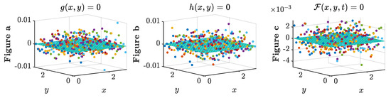
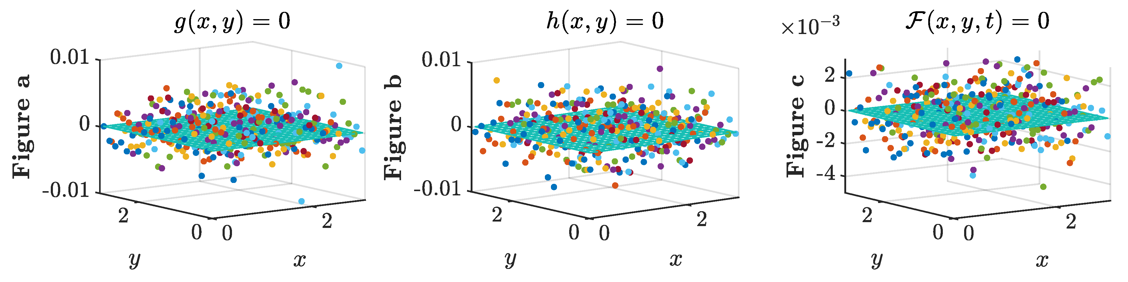
In this situation, we set $t=1/4$, $N=n-1$, $M=m-1$ and $n=m$. Observation value of $\mathcal{F}$, g, h follow the random models, see Figure 1,

$${\widehat{\mathcal{F}}}_{ij}(t)=\frac{1}{\sqrt{nm}}{\mathcal{B}}_{ij}(t),{\widehat{g}}_{ij}=\frac{1}{\sqrt{nm}}{\xi }_{ij},{\widehat{h}}_{ij}=\frac{1}{\sqrt{nm}}{\chi }_{ij},i=1,\dots ,n,j=1,\dots ,m.$$

Figure 1. The exact data $g(x,y)=h(x,y)=\mathcal{F}(x,y,t)$ and their observation value at time $t=1/4$.

The value of $\mathit{D}(t)$ and $\mathit{S}(t)$ are given in Table 1. Through this result, we clearly see that the smaller $D(1/4)$, the larger $S(1/4)$ will be, when $n=m$ increases from 5 to 50.

Table 1. A small change in the data result in a large change in the solution.

	$\mathit{n}=\mathit{m}=5$	$\mathit{n}=\mathit{m}=10$	$\mathit{n}=\mathit{m}=20$	$\mathit{n}=\mathit{m}=50$
$\mathbf{D}(1/4)$	0.5685	0.1799	0.0501	0.0085
$\mathbf{S}(1/4)$	0.5800	1.7333 × 10${}^3$	1.9078 × 10${}^{10}$	1.7587 × 10${}^{35}$

6.2. Convergence Behavior of the Regularized Solution

In this section, we present an example in order to illustrate the efficiency of the proposed methods. We consider following Cauchy problem:

$$\left\{\begin{array}{cccccc}\hfill u_{tt}+u_{xx}+u_{yy}& =& \mathcal{F}(x,y,t),\hfill & \hfill (x,y,t)& \in & \mathsf{\Omega }\times (0,1),\hfill \\ \hfill u(x,y,0)& =& g(x,y),\hfill & \hfill (x,y)& \in & \mathsf{\Omega },\hfill \\ \hfill u_t(x,y,0)& =& h(x,y),\hfill & \hfill (x,y)& \in & \mathsf{\Omega },\hfill \end{array}\right.$$

where $\mathcal{F}(x,y,t)=-2tsinxsiny$, $g(x,y)=0$ and $h(x,y)=sinxsiny$. This system has the exact solution $u(x,y,t)=tsinxsiny$.

The observation data at grid points $(x_i,y_j)=\left(\pi \frac{2i-1}{2n},\pi \frac{2j-1}{2m}\right)$; $i=1,\dots ,n$; $j=1,\dots ,m$ of functions $\mathcal{F},h,g$ are

$$\begin{array}{cc}{\widehat{\mathcal{F}}}_{ij}(t)\hfill & =\mathcal{F}(x_i,y_j,t)+\alpha {\mathcal{B}}_{ij}(t),\alpha =1\mathrm{and}{\mathcal{B}}_{ij}(t)\stackrel{i.i.d}{\sim }N(0,1),\hfill \\ {\widehat{g}}_{ij}\hfill & =g(x_i,y_j)+{\sigma }_{ij}{\xi }_{i,j},{\sigma }_{ij}=0.1\mathrm{and}\xi ij\stackrel{i.i.d}{\sim }N(0,1),\hfill \\ {\widehat{h}}_{ij}\hfill & =h(x_i,y_j)+{\upsilon }_{ij}{\chi }_{ij},{\upsilon }_{ij}=0.1\mathrm{and}{\chi }_{ij}\stackrel{i.i.d}{\sim }N(0,1),\hfill \end{array}$$

for all $i=1,\dots ,n$; $j=1,\dots ,m$. For fixed t, the matrix form of the regularized solution will be

$${\mathcal{U}}^{N,M}=\left[\begin{array}{cccc}{\mathcal{U}}^{N,M}(x_1,y_1,t)& {\mathcal{U}}^{N,M}(x_1,y_2,t)& \cdots & {\mathcal{U}}^{N,M}(x_1,y_m,t)\\ {\mathcal{U}}^{N,M}(x_2,y_1,t)& {\mathcal{U}}^{N,M}(x_2,y_2,t)& \cdots & {\mathcal{U}}^{N,M}(x_2,y_m,t)\\ ⋮& ⋮& ⋮& ⋮\\ {\mathcal{U}}^{N,M}(x_n,y_1,t)& {\mathcal{U}}^{N,M}(x_n,y_2,t)& \cdots & {\mathcal{U}}^{N,M}(x_n,y_m,t)\end{array}\right],$$

the elements of ${\mathcal{U}}^{N,M}$ are computed as

$$\begin{array}{ll}{\mathcal{U}}^{N,M}(x_i,y_j,t)={\displaystyle \sum _{p=1}^N}{\displaystyle \sum _{q=1}^M}\hfill & \left[cosh\left(t\sqrt{{\lambda }_{p,q}}\right){\widehat{g}}_{n,m;p,q}^{N,M}+\frac{sinh\left(t\sqrt{{\lambda }_{p,q}}\right)}{\sqrt{{\lambda }_{p,q}}}{\widehat{h}}_{n,m;p,q}^{N,M}\right.\hfill \\ \\ \left.+{\int }_0^t{\displaystyle \frac{sinh\left(\sqrt{{\lambda }_{p,q}}(t-s)\right)}{\sqrt{{\lambda }_{p,q}}}}{\widehat{\mathcal{F}}}_{n,m;p,q}^{N,M}(s)\mathrm{d}s\right]{\phi }_{p,q}(x_i,y_j).\hfill \end{array}$$

The errors are esimated by

$$Er{r}_{n,m}^{N,M}(t)=\sqrt{\frac{1}{nm}{\displaystyle \sum _{i=1}^n}{\displaystyle \sum _{j=1}^m}{\left[{\mathcal{U}}^{N,M}(x_i,y_j,t)-u(x_i,y_j,t)\right]}^2}.$$

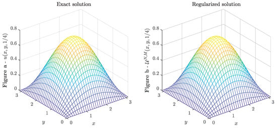
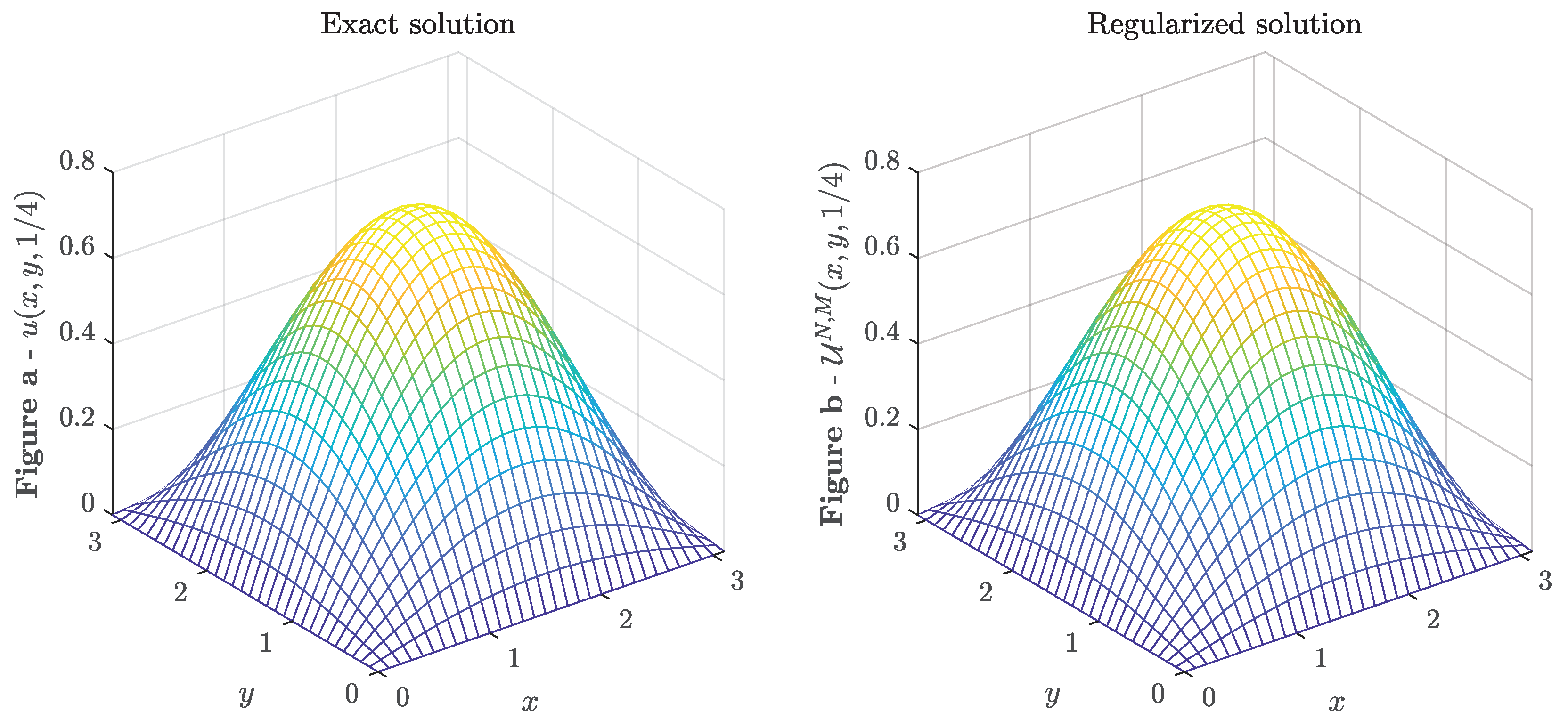
In this numerical example, we keep the fixed value of regularization parameters with $N=M=3$. We carried out the numerical calculations for two cases with different observation points; the first one for $n=m=500$, and another one for $n=m=1000$. From Table 2, it shows that the error is reduced once the spatial observation points are increased; on the other hand the convergence rate has been increased once time t tends to 0. This reflects the behavior of the rate of convergence in Theorem 1. For a more intuitive look, in Figure 2, we show the 3D graphs of the exact solution and regularized solution at $t=1/4$, where we chose $N=M=3$ and $n=m=1000$.

Table 2. Numerical errors

${\mathit{Err}}_{\mathit{n},\mathit{m}}^{\mathit{N},\mathit{M}}(\mathit{t})$	$\mathit{t}=1/4$	$\mathit{t}=1/2$	$\mathit{t}=3/4$	$\mathit{t}=1$
$n=m=500$	7.92 × 10${}^{-4}$	1.51 × 10${}^{-3}$	3.60 × 10${}^{-3}$	1.27 × 10${}^{-2}$
$n=m=1000$	4.91 × 10${}^{-4}$	7.75 × 10${}^{-4}$	1.50 × 10${}^{-3}$	3.31× 10${}^{-3}$

Figure 2. 3D graphs of exact solution at time $t=1/4$, and the regularized solution for the regularization parameters of $N=M=3$ and $n=m=1000$.

7. Conclusions

In this work, we considered the problem of finding the solution for the 2-D inhomogeneous elliptic equation with initial data and source pertubed by random noise. We first estimate the initial functions and source function using the nonparametric least square regression method in statistic manner. Then we approximated Fourier coefficients $f_{p,q}$ by $f_{n,m;p,q}$ which is the function of the data set. This problem is ill-posed, hence a regularization is needed. Eventually, we have carried out the numerical example, and validated the regularized solution against the exact solution, it shows the numerical errors have been reduced once the number of spatial observation points is increased; on the other hand the convergence rate is increased once t tends to zero.

References

- Lavrentev, M.M.; Romanov, V.G.; Shishatskii, S.P. Ill-posed Problems of Mathematical Physics and Analysis; Translations of Mathematical Monographs; American Mathematical Society: Providence, RI, USA, 1986; Volume 64. [Google Scholar]
- Heyvaerts, J.; Lasry, J.M.; Schatzman, M.; Witomski, P. Solar flares: A non linear eigenvalue problem in an unbounded domain. In Bifurcation and Nonlinear Eigenvalue Problems; Lecture Notes in Mathematics 782; Springer: Berlin, Germany, 1980; pp. 160–191. [Google Scholar]
- Johnson, C.R. Computational and numerical methods for bioelectric field problems. Crit. Rev. Biomed. Eng. 1997, 25, 1–81. [Google Scholar] [CrossRef] [Scilit] [PubMed]
- Tuan, N.H.; Thang, L.D.; Khoa, V.A. A modified integral equation method of the nonlinear elliptic equation with globally and locally Lipschitz source. Appl. Math. Comput. 2015, 256, 245–265. [Google Scholar] [CrossRef] [Scilit]
- Tuan, N.H.; Binh, T.T.; Viet, T.Q.; Lesnic, D. On the Cauchy problem for semilinear elliptic equations. J. Inverse Ill-Posed Probl. 2016, 24, 123–138. [Google Scholar] [CrossRef] [Scilit]
- Haase, M. Functional Analysis: An Elementary Introduction; American Mathematical Society: Providence, RI, USA, 2014. [Google Scholar]
- Eubank, R.L. Nonparametric Regression and Spline Smoothing; CRC Press: Boca Raton, FL, USA, 1999. [Google Scholar]
- Salsa, S. Partial Differential Equations in Action From Modelling to Theory; Springer: Berlin, Germany, 2008. [Google Scholar]
- Hunter, J.K.; Nachtergaele, B. Applied Analysis; World Scientific Publishing Company: Singapore, 2001. [Google Scholar]
© 2019 by the authors. Licensee MDPI, Basel, Switzerland. This article is an open access article distributed under the terms and conditions of the Creative Commons Attribution (CC BY) license (http://creativecommons.org/licenses/by/4.0/).