Regional Coordinated Traffic Signal Control Based on Improved Chaotic Particle Swarm Optimization

Abstract

In urban traffic systems, traditional signal control can no longer meet the increasing traffic demand, and local congestion is severe during peak hours. Fixed detector data is characterized by high deployment density, full sample detection and restorable vehicle paths, providing new data support for coordinated signal control. We propose an optimization method for regional coordinated control, with the Changsha road network as the study area. Firstly, based on License Plate Recognition (LPR) data, the road network is divided into sub-networks and combined with the boundary control for regional coordinated control. Then, the critical path is taken as the control object, and the phase coordination rate is introduced as the optimization objective. The particle swarm optimization algorithm improved by the logistic chaotic map is used as the global searcher, and sequential quadratic programming is adopted as the local searcher to solve the optimization strategy for the objective function. Finally, a simulated road network is constructed in VISSIM 6.0 simulation software to verify the effectiveness of the strategy. The results show that the optimization strategy reduces intersection delay and saturation by 20.3% and 19.3% in the critical path coverage area. Road travel time and the average number of vehicle stops are reduced by 21% and 22.1%. This indicates that the regional coordinated control based on the improved particle swarm algorithm can better alleviate the peak hour traffic congestion.

1. Introduction

Signalized intersections play a critical role in managing and controlling urban traffic. In a high-traffic environment, traditional timing control cannot meet the traffic demand. The resulting bottlenecks also limit traffic efficiency. Therefore, the optimization of urban traffic control strategies often focuses on intersection signal management [1,2,3,4]. To address the challenges posed by intersection traffic flow, a range of innovative control methods have been developed, including inductive control and dynamic control, among others. These control strategies are usually tightly coupled to the historical data of the intersection, so that control strategies calibrated with actual data are more effective than traditional fixed-time control.

However, with the rapid development of cities, the area of the road network is expanding and the volume of traffic is increasing. The vast amount of data makes computation difficult, hindering large-scale coordinated control. For large-scale road networks, the first step in coordinated control should be to reduce complexity while ensuring effectiveness. To solve the problem, many scholars have conducted research from the perspective of sub-network control. The results have shown that control efficiency can be improved by dividing a large road network into several sub-networks prior to coordinated control. To improve the effectiveness of coordinated control, researchers try to find the optimal solution of coordinated control according to different control objectives, which can be divided into two categories: optimal efficiency and maximum bandwidth. Among the former, the effectiveness of coordinated control is mostly measured by indicators such as delays and number of stops. The method is based on assumptions and modeling to characterize the control effects under different parameters. However, the actual control benefits are influenced by many factors, making it difficult to apply accurately. In contrast, coordinated control based on bandwidth maximization has the advantages of simple inputs and low influence of other factors, but is mainly suitable for arterial roads rather than large-scale regional networks.

In addition, suitable optimization models can also improve the effectiveness of the optimization strategy, and common methods include: genetic algorithms, cellular models, simulated annealing algorithms, particle swarm optimization, and so on. As a heuristic algorithm, particle swarm optimization has a rapid convergence rate and straightforward parameters, making it suitable for the optimization of practical problems. However, its global search ability is insufficient, which may lead to the problem of premature convergence, and the integration of stochastic theory can address this limitation.

In order to explore the impact of different coordinated control methods on large-scale urban road networks, the study takes Changsha city road network as the research object and extracts vehicle data from the LPR system as the database. Firstly, the road network is divided into sub-networks based on vehicle data and actual road parameters, and boundary control is applied at the boundaries of sub-networks. In the optimization model, the phase coordination rate is taken as the optimization objective. Based on particle swarm optimization, logistic chaotic mapping is introduced to form the global searcher. And sequential quadratic programming is used as the local searcher to strengthen the algorithm accuracy. Finally, the solved optimization scheme is applied to the simulated road network constructed by VISSIM 6.0 to analyze the optimization effect. The main contributions of this study are: (1) a data-driven network partitioning method using LPR trajectories that better reflects real traffic distribution; (2) phase coordination rate as an optimization objective, which is more suitable for large-scale networks than bandwidth-based indicators; (3) an improved hybrid PSO algorithm combining logistic chaotic mapping and SQP for better global and local search; (4) a complete coordinated control framework integrating partitioning, boundary control, and multi-intersection coordination; and (5) empirical validation using real LPR data from Changsha and VISSIM simulation.

2. Literature Review

2.1. Regional Coordinated Control

As the scope of the urban road network expands and the number of motor vehicles increases, research on regional travel is increasing. Reasonable area divisions are the basis for studying regional travel.

In the implementation of urban road network control, if vehicle density varies significantly across the network, control efficiency will be reduced. Therefore, in order to improve the control efficiency of road networks, many scholars have conducted research from the perspective of road network division. Ji et al. [5] developed a segmentation method comprising three key components: a normalized segmentation, a merging algorithm based on the initial segmentation, and a boundary adjustment algorithm. This method has the potential to enhance the quality of road network segmentation. Saeedmanesh et al. [6] proposed a snake clustering algorithm that considers road dependencies, similarities between roads, and the size of sub-networks. The method achieves homogeneous network segmentation. Lopez et al. [7] compared and contrasted the k-means algorithm, density-based segmentation, and snake clustering segmentation in an urban road network environment. The k-means algorithm was determined to be more advantageous in terms of the division results. Lukas et al. [8] proposed an inhomogeneous network division algorithm using traffic information collected by stationary sensors. The method generates several possible division results. Then, a homogeneity analysis is performed based on the corresponding MFD. Finally, the division result with the highest homogeneity is filtered as the solution of the algorithm. Yang et al. [9] extracted traffic features under different spatio-temporal conditions using tensor decomposition. A spectral clustering approach was used to divide the large road network into independent sub-networks with similar levels of congestion. Hu et al. [10] developed a correlation model for adjacent intersections on arterial roads based on vehicle detection data. The model was able to quantify the correlation of intersections more accurately. Then, the road network was divided using a zoning method based on the correlation indicator, and the results showed that the method could significantly improve the operational efficiency of arterial roads. Dimitriou et al. [11] investigated the effect of different division methods on road network delineation. They pointed out that data-based clustering methods have some limitations in road network division. Using a graph-based segmentation method can better divide the road network. Niu et al. [12] proposed a spatio-temporally integrated road network delineation method based on density clustering. This method takes into account the spatio-temporal characteristics of traffic flow and can dynamically divide the road network. Wen et al. [13] improved the road network delineation method for unsaturated traffic state. The new correlation model was constructed by integrating physical distance, flow rate, and queue length. By simulating in the simulation environment, it was concluded that the road network division results based on the DBSCAN algorithm were closer to the actual situation.

After segmentation of the road network has been completed, coordinated control of the sub-networks is required. Aboudolas et al. [14] designed three signal control strategies for massively congested urban road networks using control and optimization methods. de Oliveira et al. [15] proposed an urban road network control method based on model predictive control. The method is an improvement of traffic-responsive urban control. However, with the complexity of the city scale, the optimization problem of traffic signals becomes more and more complicated. Many scholars have proposed layered control architectures. Hajbabaie et al. [16] proposed a hierarchical control based on signal timing optimization and traffic assignment. A new objective function was proposed for saturated traffic networks to improve the system performance. Feng et al. [17] optimized a two-layer control model. The green light time extremes were improved in the upper-layer model, and the phase order and green light time were optimized in the lower-layer model. Huang et al. [18] proposed a three-layer hierarchical model-based approach for network-wide traffic signal control. This method divides regional coordinated control into three layers: the regional coordination layer, the intersection coordination layer, and the local signal coordination layer. The results show that this approach can reduce computational complexity while maintaining the overall performance of the road network. In recent years, advancements in machine learning have led many researchers to apply these techniques to cooperative control [19,20]. While they have demonstrated the effectiveness of their proposed methods in reducing local delays and improving traffic network efficiency, some new limitations have also emerged.

In the above study, for the coordinated control of large-scale road networks, the idea of optimization mainly to make it smaller first, and then apply the control. That is to say, firstly, the road network is divided into sub-networks. Second, coordinated control is applied to the sub-networks to improve the operational efficiency. The method can also be applied to key sub-networks and key intersections in the road network to achieve similar optimization results.

2.2. Particle Swarm Optimizations for Traffic Control

Particle swarm optimization (PSO) is a stochastic search algorithm based on group cooperation, which was developed by simulating the foraging behavior of flocks of birds. The method has many advantages such as simple operation, fast convergence, few parameters and easy adaptation, etc. Therefore, it has been applied in many fields of optimization. The application of PSO in traffic control mainly includes signal optimization [21,22], path navigation [23], vehicle deployment [24], flow control [25,26] and other aspects. The application of PSO in traffic control reflects its strong optimization ability and adaptability. By simulating the cooperation and competition mechanism in the foraging behavior of flocks of birds, PSO can effectively solve the complex optimization problems in traffic control and improve the efficiency and performance of the traffic system.

Garcia-Nieto et al. [27] used PSO to find an optimization scheme for signal control. They optimized the number of vehicles reaching the destination and the total travel time. The simulation results show that the method is able to obtain a more efficient signal control scheme. Hatri et al. [28] proposed a traffic control model based on multi-objective particle swarm optimization. The model can be used to optimize both vehicle path and signal control. Zhang et al. [29] proposed an expressway traffic control method combining ramp control and variable speed limit, using the PSO algorithm to search for optimal signals for coordinated control schemes. Qin et al. [30] incorporated the chaos algorithm and agent interaction techniques into the traditional PSO algorithm. It achieves the collaborative decision-making of multiple intersections. The method can speed up the convergence of the optimization algorithm while improving the overall traffic efficiency. The study by Olivera et al. [31] is based on a sustainable development perspective. In the selection of optimization objects, not only are motor vehicles considered, but pedestrian traffic flow is also optimized, which is relatively rare in urban traffic control. Yuen et al. [32] proposed an improved multi-objective PSO algorithm with a competitive mechanism. Compared with the commonly used multi-objective particle swarm algorithms, the improved computation with the introduction of a competitive mechanism can optimize the control effect more effectively, especially in the hypervolume traffic problem. Yong et al. [33] improved the PSO algorithm by utilizing the idea of natural selection in a genetic algorithm. The joint simulation results of VISSIM 5.2 and MATLAB show that the improved particle swarm algorithm can improve the passing efficiency of transit traffic flow. Subrahmanyam et al. [34] optimized Ant Colony Optimization (ACO) and PSO algorithms from an IoT perspective. In their proposed algorithms, ACO can select the best driving route during peak traffic hours. Meanwhile, the PSO algorithm can optimize speed, avoid congestion, and save travel time. The computational results also show that the integration of ACO and PSO algorithms can improve the effectiveness of traffic management.

Currently, particle swarm optimization (PSO) remains the mainstream intelligent optimization method in the field of regional traffic coordination control, with research focusing on multi-objective optimization [35], adaptation to engineering constraints [36], and hybrid intelligent frameworks [30]. Relevant findings indicate that improved Particle Swarm Optimization algorithms demonstrate superior optimization performance when addressing the dynamics of road networks and multi-intersection coordination problems, effectively enhancing control outcomes and providing a viable approach for signal timing optimization in complex traffic scenarios.

2.3. Traffic Flow Research Based on Chaos Theory

Chaos is a complex dynamic system. It is characterized by nonlinearity and randomness, which provide the complexity of the system. Chaotic signals generated by such systems are also characterized by initial value sensitivity and noise-like properties. They play an important role in mathematics, computer science, cryptography and other disciplines. Chaotic property analysis is also very common in traffic flow data. The main research method is to use a chaotic discrimination method to discriminate the data. The differences between existing studies are mainly in the discriminating method or the type of traffic flow data.

Due to the limitations of the actual environment, the changes in each parameter of the traffic flow are difficult to fully record in the actual collection process. Therefore, many scholars select a theoretical model of traffic flow as the basis, use simulation software to build a simulation road network, and change the parameters of the model to explore the change rules of chaotic phenomena.

On the basis of the research on chaos phenomena, chaos theory has also been applied to traffic control. Keiji Konishi et al. [37] extracted the proportional components of front and rear vehicle speeds as feedback control signals based on a simple tracking model with delayed feedback to realize the purpose of traffic flow chaos control. A multi-layer chaotic neural network involving feedback has been proposed by Dong et al. [38]. Optimizing signal timing using this method can effectively reduce vehicle delay. Zhao et al. [39] simplified the four control variables in Keiji’s study to one control variable to control for the chaotic nature of traffic flow. According to the study by Narh et al. [40], the application of chaos theory to urban traffic control is very reliable. It can detect the occurrence of congestion. Influenced by data sources, its application has mainly been focused on highways and relatively simple intercity roads in the past. The emergence of high-resolution data sources and large data storage capacity will overcome this problem. Therefore, in the future, chaos theory will enable traffic control in more complex road environments to prevent and improve congestion. For instance, Qin et al. [30] proposed a chaotic particle swarm optimization (CPSO) that combines a chaos algorithm with agent-based cooperative control technology for multi-intersection signal timing optimization, using vehicle delay, queue length, and regional access ratio as optimization objectives, showing how chaos theory can be directly integrated into traffic signal control algorithms. Zhong et al. [41] developed a neural network-based adaptive control for the Aw–Rascle–Zhang mixed traffic flow model under unknown external disturbances, demonstrating how nonlinear traffic dynamics can be effectively regulated. These studies provide a basis for chaotic control of traffic flow, but the studies use more assumptions that differ from actual traffic flow and are more difficult to apply.

3. Methodology

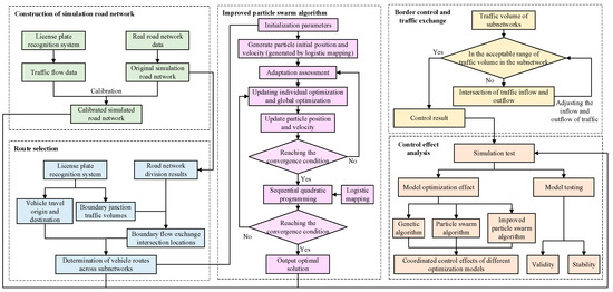
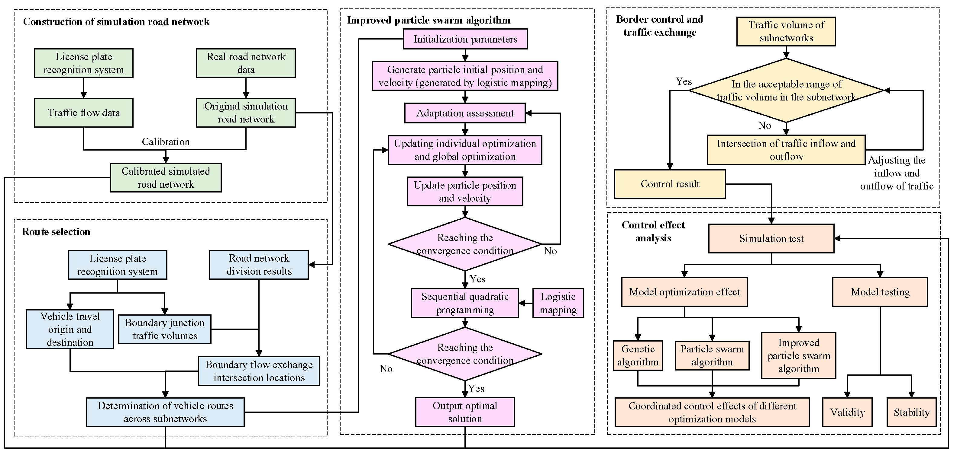
The following figure (Figure 1) illustrates the research process outlined in the study. Initially, a calibrated simulated road network can be generated based on the data in the LPR system and the real road network. The network can then be utilized to verify the control effect. The data in the LPR system can be used to ascertain the origin and destination of the traveling vehicle. Furthermore, the results of the sub-network division can be integrated with the information to determine the route of the vehicle traveling through the sub-network. Subsequently, particle swarm optimization is employed to optimize the route in accordance with the parameters of the origin and destination of the route and the state of the road network. Upon reaching the convergence condition, the optimal route is output. The results are then substituted into the simulated road network. The coordinated control of the road network is performed by the two-layer model and sub-network boundary control. Finally, the effects of different optimization models on the coordinated control are analyzed, and the effectiveness of the model is verified.

Figure 1. Scheme of traffic control process.

3.1. Bilevel Control Model

3.1.1. Back Pressure Value

In a two-layer control model, the upper layer model needs to select a traffic parameter that can characterize the operational state of the road network. Based on the results of existing studies, back pressure control can be applied to signal control at a single intersection because it identifies the maximum pressure value. Consequently, in the study, the back pressure value is employed as a characterization index for road sections, intersections, and road networks. The corresponding equations are presented in Equations (1)–(3), respectively.

$$w_{l,m}\left(k\right)=x_{l,m}\left(k\right)-{\displaystyle {\sum }_{h\in o_m}}{r}_{m,h}\left(k\right)x_{m,h}\left(k\right)$$

(1)

where $x_{l,m}\left(k\right)$ denotes the number of vehicles traveling from road l to road m at time k, $r_{m,h}\left(k\right)$ denotes the turning rate from road l to road m from time k to k + 1, $r_{m,h}\left(k\right)\in \left(0,1\right)$, and $o_m$ denotes the downstream ensemble of road m.

$$p_u\left(k\right)={\displaystyle {\sum }_{u_u\in U_u}}{\displaystyle {\sum }_{\left(l,m\right)\in u_u}}{w}_{l,m}\left(k\right)s_{l,m}\left(k\right)c_{l,m}\left(k\right)$$

(2)

where $U_u$ represents the set of phases of intersection u, $u_u$ represents the phase of intersection u,${ s}_{l,m}\left(k\right)$ represents the signal value from road l to road m from time k to k + 1, and $c_{l,m}\left(k\right)$ represents the saturation flow rate of the traffic flow from road l to road m from time k to k + 1.

$$\gamma \left(k\right)=\sum {\delta }_l{w}_l\left(k\right)$$

(3)

where ${\delta }_l$ is the weighting factor of road l, which is used to balance the delay time of different sections in the road network.

3.1.2. Upper-Level Model

For the upper-level model, the optimization objective is the optimal back pressure value of the road network, as shown in Equation (4). In the constraints, for intersection u, the phase $u_n$ at time k has two forms of open or closed, corresponding to the values of 1 and 0. The cumulative sum of the phase $u_n$ for the whole intersection at time k is 1. It is guaranteed that only a single phase is in the open state, as shown in Equation (5).

For most road sections, there are both arriving and departing vehicles at a given time. Considering only the back pressure value could potentially result in a situation where the road capacity is exceeded, resulting in a meaningless solution. Therefore, it is necessary to constrain the road capacity as shown in Equation (6).

$$\mathit{max}Z=\gamma \left(k\right)$$

(4)

$$\sum u_n\left(k\right)=1$$

(5)

$$x_{l,m}\left(k+1\right)=x_{l,m}\left(k\right)+z_{l,m}\left(k\right)-h_{l,m}\left(k\right)$$

(6)

where $x_{l,m}\left(k\right)$ denotes the number of vehicles traveling from road l to road m in time k, $z_{l,m}\left(k\right)$ denotes the traffic demand of path p from time k to time k + 1, and $h_{l,m}\left(k\right)$ denotes the number of vehicles traveling from road l to road m within times k to k + 1.

3.1.3. Lower-Level Model

For the lower-level model, the goal is to make decisions about the timing of traffic signals at intersections within the road network. During peak hours, some intersections are highly saturated. In the case, using Webster’s timing method significantly increases vehicle delays. Therefore, we consider incorporating intersection capacity maximization and vehicle delay minimization as objective functions while using the effective green time constraint. This could improve the applicability of the method in highly saturated environments. The calculation method is defined as follows:

$$\mathit{max}Q={\displaystyle {\sum }_{i=1}^n}{\displaystyle {\sum }_{j=1}^{m_i}}{S}_{ij}{\displaystyle \frac{g_i}{C}}$$

(7)

$$\mathit{min}d={\displaystyle \frac{{\sum }_{i=1}^n{\sum }_{j=1}^{m_i}{q}_{ij}{d}_{ij}}{{\sum }_{i=1}^n{\sum }_{j=1}^{m_i}{q}_{ij}}}$$

(8)

$${\displaystyle \frac{y_i}{Y}}\left(C_{min}-L\right)\le g_i\le {\displaystyle \frac{y_i}{Y}}\left(C_{max}-L\right)$$

(9)

where $Q$ is the intersection capacity, n is the number of phases, $m_i$ is the number of lane groups in phase i, $S_{ij}$ is the saturation flow rate of lane group j in phase i, $g_i$ is the effective green time in phase i, $C$ is the signal cycle time, $d$ is the average delay per vehicle at the intersection, $q_{ij}$ is the flow rate of lane group j in phase I, $d_{ij}$ is the average delay for lane group j in phase i,$y_i$ is the flow rate in phase i, $Y$ is the total flow rate at the intersection, $L$ is the total lost time per cycle,$C_{min}$ is the minimum cycle time, and ${ C}_{max}$ is the maximum cycle time.

3.2. Phase Coordination Rate

Traditional coordinated control methods often use bandwidth maximization as the optimization objective. Bandwidth measures the continuous green time window for vehicles traveling along an arterial at a constant speed. However, in large-scale regional networks, vehicles do not maintain constant speeds, and the network topology is not linear. These factors make bandwidth conceptually ambiguous and computationally challenging to apply directly. Therefore, this study introduces the phase coordination rate as an alternative optimization objective. Unlike bandwidth, the phase coordination rate is a pairwise, data-driven metric that measures, for each pair of adjacent intersections, the proportion of upstream vehicles that arrive during the downstream green time. It does not assume constant speeds or linear topology, making it naturally scalable to regional networks.

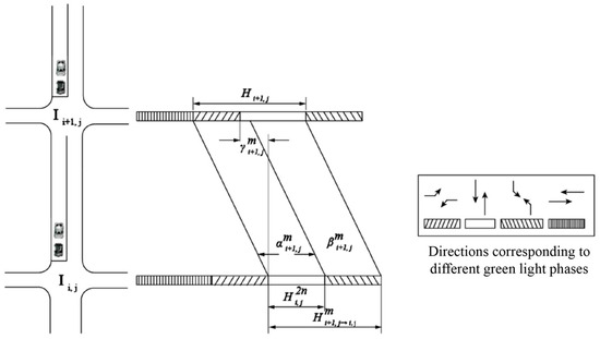
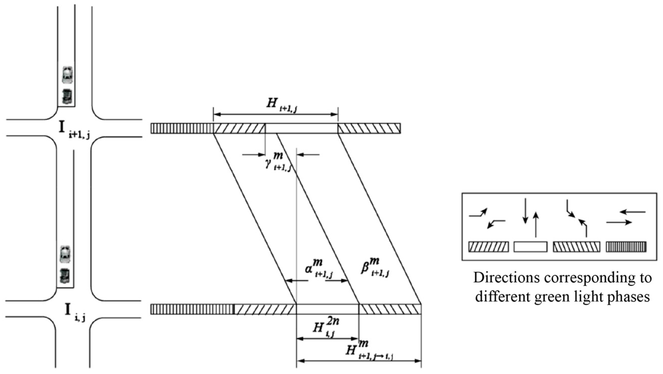
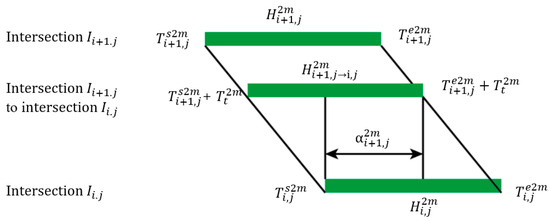
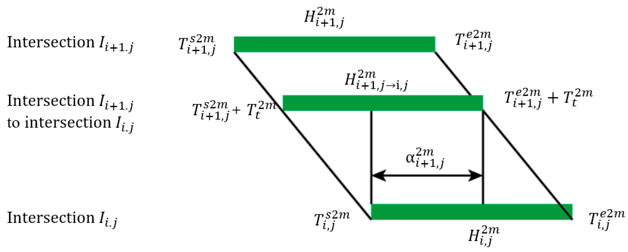
The concept of phase coordination rate is applied to two neighboring intersections, and Figure 2 shows the phase timing diagram for two neighboring intersections.

Figure 2. Phase time diagram.

Taking north–south traffic as an example, assuming that the green light time in the mth cycle is $H^m$, there is a corresponding $H_{i+1,j}^m$ for intersection $I_{i+1.j}$. And $H_{i+1,j\to i,j}^m$ denotes the mapped green time of the intersection $I_{i+1.j}$ at the intersection $I_{i.j}$, whereas $H_{i,j}^{2n}$ denotes the green time of the nth cycle of intersection $I_{i.j}$ in the north–south direction.

${\alpha }_{i+1,j}^m$ denotes the part of $H_{i+1,j\to i,j}^m$ that overlaps with $H_{i,j}^{2n}$, i.e., the amount of phase coordination. ${\gamma }_{i+1,j}^m$ is the phase difference between the mth cycle of the upstream intersection and the corresponding phase of the downstream intersection. ${\beta }_{i+1,j}^m$ donates the part of $H_{i+1,j\to i,j}^m$ that does not overlap with $H_{i,j}^{2n}$. For ${\alpha }_{i+1,j}^m$, dividing it by $H_{i+1,j\to i,j}^m$, the larger the value, the more likely it is that the upstream intersection traffic will be in the green time when it arrives downstream. The concept is known as the phase coordination rate ${\delta }_{i+1,j\to i,j}^m$, as shown in Equation (10).

$${\delta }_{i+1,j\to i,j}^m={\displaystyle \frac{{\alpha }_{i+1,j}^m}{H_{i+1,j}^m}}$$

(10)

Similarly, for the intersection $I_{i-1.j}$ downstream of the intersection $I_{i.j}$, there exists ${\alpha }_{i-1,j}^{\mathrm{m}}$ and ${\delta }_{i-1,j\to i,j}^m$ from the south to the north, and its calculation equation is as follows:

$${\delta }_{i-1,j\to i,j}^m={\displaystyle \frac{{\alpha }_{i-1,j}^m}{H_{i-1,j}^m}}$$

(11)

In signal coordination for intersection $I_{i.j}$, if ${\delta }_{i-1,j\to i,j}^m$ and ${\delta }_{i+1,j\to i,j}^m$ correspond to the same phase, the smaller of the two is chosen as the coordination rate ${\delta }_{i,j}^m$.

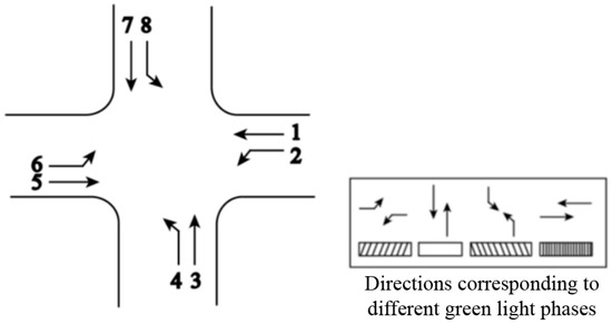
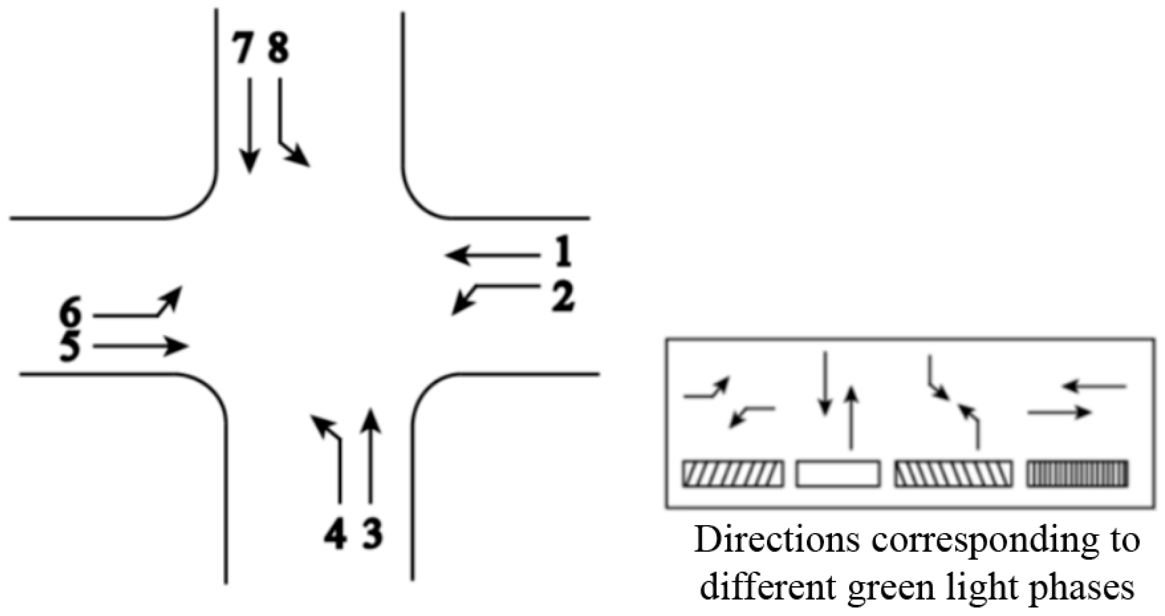
After obtaining the phase coordination rates for individual directions, the phase coordination rates for intersections can be further derived. Figure 3 represents each turn and phase at the intersection, and Table 1 shows the numbering of each lane corresponding to the phase coordination rate. Figure 4 displays the green time projection relationship between two adjacent intersections.

Figure 3. Diagram of intersection phase sequence.

Table 1. Phase coordination rate coding rules.

Direction Number	1	2	3	4	5	6	7	8
phase coordination rate	${\delta }_q^{4m}$	${\delta }_{\mathrm{q}}^{1m}$	${\delta }_q^{2m}$	${\delta }_q^{3m}$	${\delta }_p^{4m}$	${\delta }_p^{1m}$	${\delta }_p^{2m}$	${\delta }_p^{3m}$

p: i + 1, j → i, j; q: i − 1, j → i, j.

Figure 4. Relationship of green time mapping.

From Figure 4, we can get ${\alpha }_{i+1,j}^{2m}$ as in Equation (12).

$${\alpha }_{i+1,j }^{2m}={ H}_{i+1,j\to i,j}^{2m}\cap H_{i,j}^{2m} =min\left(T_{i+1,j}^{e2m}+T_t^{2m},{ T}_{i+1,j}^{e2m} \right)-max(T_{i+1,j}^{s2m}+T_t^{2m}, T_{i+1,j}^{s2m})$$

(12)

In addition, the intersecting roads forming an intersection may be of different classes and the signal cycle time may not be consistent. Therefore, ${\sigma }_{i,j}$ is introduced to represent the number of cycles that intersection $I_{i.j}$ goes through in a large cycle $C_{i,j}^{i+1,j}$. The value of $C_{i,j}^{i+1,j}$ is taken as the least common multiple of the intersections $I_{i.j}$ and $I_{i+1.j}$. Equation (12) can be derived from Equations (13) and (14).

$${\sigma }_{i,j}={\displaystyle \frac{C_{i,j}^{i+1,j}}{C_{i,j}}}$$

(13)

$${\delta }_{i+1,j\to i,j}^{2m}={\displaystyle \frac{{\alpha }_{i+1,j}^{2m}}{{{\sigma }_{i+1,j}H}_{i+1,j}^{2m}}} ={\displaystyle \frac{{\alpha }_{i+1,j}^{2m}}{{\sigma }_{i+1,j}\left(g_{i+1,j}^1+g_{i+1,j}^2\right)}}$$

(14)

Similarly, the coordination rate ${\delta }_{i,j}^{2m}$ for the north–south straight at intersection $I_{i.j}$ is determined by the lower rate of the coordination rate ${\delta }_{i+1,j\to i,j}^{2m}$ for intersection $I_{i+1.j}$ and the coordination rate ${\delta }_{i-1,j\to i,j}^{2m}$ for intersection $I_{i-1.j}$.

The coordination rates for the other three phases can also be derived and are denoted by ${\delta }_{i,j}^{1m}$, ${\delta }_{i,j}^{3m}$, and ${\delta }_{i,j}^{4m}$. The phase coordination rate for the intersection $I_{i.j}$ is shown in Equation (15).

$$g\left(I_{i.j}\right)={{\tau }_1\delta }_{i,j}^{1m}+{\tau }_2{\delta }_{i,j}^{2m}+{{\tau }_3\delta }_{i,j}^{3m}+{\tau }_4{\delta }_{i,j}^{4m}$$

(15)

$\tau$ is the phase weight ratio, for intersections with high saturation, the value of phase weight should be determined in conjunction with the operation status of the intersection. First, under the same phase, the maximum traffic flow among all traffic flows is selected as the weight value. Then, under different phases, the weight ratio value is the ratio of the maximum traffic flow of the phase.

When using the phase coordination rate as the optimization objective for coordinated control, the main inputs and influencing factors differ from those of traditional bandwidth-based methods. Specifically, the following factors need to be considered: vehicle driving trajectories (obtained from LPR data), intersection topology, the degree of green time overlap between upstream and downstream intersections, the distribution of vehicle arrival times, and phase sequence and offset settings. These factors collectively determine the achievable coordination quality in large-scale road networks.

3.3. Improved Chaotic Particle Swarm Optimization

3.3.1. Particle Swarm Optimization

In particle swarm optimization, each solution is a particle in the search space. First of all, a set of random particles needs to be generated, and their position is defined as ${\mathrm{x}}_i={\left(x_{i1},x_{i2},\cdots ,x_{iN}\right)}^T$. Its velocity is $v_i={\left(v_{i1},v_{i2},\cdots ,v_{iN}\right)}^T$, and its extreme value is $p_i={\left(p_{i1},p_{i2},\cdots ,p_{iN}\right)}^T$. Meanwhile, the global extreme value is defined as $p_g={\left(p_{g1},p_{g2},\cdots ,p_{gN}\right)}^T$. The particle swarm optimization searches for the optimal solution by adjusting the individual extreme value $p_i$ and the global extreme value $p_g$ for update iterations. Let $f\left(x_i\right)$ denote the fitness function of particle i. The updates of velocity and position are calculated as in Equations (16) and (17).

$$v_{id}^{k+1}=w\cdot v_{id}^k+c_1\cdot rand()\cdot \left(p_{id}-x_{id}^k\right)+c_2\cdot rand()\cdot \left(p_{gd}-x_{id}^k\right)$$

(16)

$$x_{id}^{k+1}=x_{id}^k+v_{id}^{k+1}$$

(17)

where i = 1, 2, … M, M is the total number of particles, d = 1, 2, …, N, N is the dimension of the solution space, i.e., the number of independent variables, k is currently the number of iterations, $k_{max}$ denotes the maximum number of iterations, $w$ is inertia weight, and rand () is a random variable that is independent and follows a uniform distribution in [0, 1], and $c_1$ and $c_2$ are acceleration factors that control the maximum step size of the flight towards $p_i$ and $p_g$, respectively. Although the classical particle swarm optimization has a fast initial convergence speed, the search speed is slow and the accuracy is not high when approaching the extremes, which leads to easy falling into the local optimum. Also, the rapid loss of species diversity can cause the algorithm to mature prematurely, so chaotic mapping is introduced to improve the shortcomings of the typical particle swarm optimization.

3.3.2. Chaos Mapping

Due to its ergodicity and stochasticity, chaotic strategies are often used in optimization and have been incorporated into particle swarm optimizations many times to help particles escape from the local optimum. When the particle swarm optimization reaches convergence, the population is chaotically mapped according to the probability $P_m$. First, all non-globally optimal particles are screened, and each particle is configured with a random number r distributed in [0, 1]. Then, it is determined whether each r is less than $P_m$. If so, a one-dimensional variable is randomly selected for the particle to perform the chaotic mapping. This paper aims to address the premature convergence problem in the standard particle swarm optimization algorithm. It employs logistic chaotic mapping. This chaotic mapping enhances the diversity of the population during the initialization stage and helps the particles escape from local optimal solutions by providing chaotic perturbations, thereby improving the global search capability. Logistic mapping is used here as an example, as in Equation (18).

$$x_{k+1}=\mu \cdot x_k\cdot \left(1-x_k\right), 0\le x_0\le 1$$

(18)

where $x_k$ is the ratio of the population to the maximum possible population size at time t, which takes values from 0 to 1; $\mu$ is the scale factor, which takes values from 0 to 4. The current particle is first recorded as the optimal solution, and the search for optimality proceeds to the next cycle. Specifically, it involves the following steps.

Step 1: For the N-dimensional variable $x_i$ to be chaotically mapped, randomly initialize the mapping subscript i between 1 and N.

Step 2: The decision variable $x_i$ is mapped to a chaotic variable $c{x}_i$ between 0 and 1 according Equation (19).

$$c{x}_i={\displaystyle \frac{x_i-x_{imax}}{x_{imax}-x_{imin}}}$$

(19)

where $x_{imax}$ and $x_{imin}$ are the upper and lower bounds of the search for the i-th dimensional variable, respectively.

Step 3: Update the chaotic variable ${cx}_i$ with Equation (18).

Step 4: The chaotic variable ${cx}_i$ is converted to the decision variable $x_i$ according to Equation (20).

$$x_i=x_{imin}+c{x}_i\left(x_{imax}-x_{imin}\right)$$

(20)

3.3.3. Sequential Quadratic Programming

Introducing chaotic mapping into particle swarm optimization can effectively improve the shortcomings of the algorithm, but it can still be optimized in terms of convergence accuracy. Therefore, we consider adding a local search to the chaotic particle swarm optimization to improve the convergence accuracy.

SQP is an optimization method for solving nonlinear planning problems. It can be used to solve extremal problems of multivariate functions with constraints. In the study, the method is incorporated into the chaotic particle swarm optimization. The chaotic particle swarm optimization is used as the global searcher and the SQP algorithm is used as the local searcher. And the optimization algorithm automatically switches between global and local search according to convergence.

First, chaotic particle swarm optimization is used to find the optimal solution. Then, taking the current optimal particle position as the starting point, SQP is called to perform local search and iterate until the termination condition is reached. To balance computational efficiency and solution quality, SQP is invoked every $f_{sqp}$ iterations. At the same time, the gradient information is used to speed up the local search during each iteration. Chaotic mapping is used to maintain the diversity of the population so that the particles can search the whole space based on fast local optimization. After the above algorithm fusion, the improved chaotic particle swarm (ICPSO) optimization based on SQP and chaotic mapping is finally formed.

3.3.4. Pseudo-Code of the Improved Algorithm

To provide a clear and complete description of the proposed hybrid optimization algorithm, Algorithm 1 presents the pseudo-code of the ICPSO integrating logistic chaotic mapping and SQP. The algorithm consists of four main steps: chaotic initialization, standard PSO iteration, chaotic perturbation, and periodic SQP refinement.

Algorithm 1: ICPSO with Logistic Chaotic Mapping and SQP
	Input: Number of particles M, dimension of solution space N, maximum iterations kmax, inertia weight w, acceleration factors c1 and c2, chaotic mapping probability Pm, scale factor μ, SQP local search frequency fsqp Output: Global extreme value pg
1	//Chaotic initialization
	Initialize cx = $x_0$ with $x_0$ ∈ (0,1);
2	for i = 1 to M do
3	for d = 1 to N do
4	Generate chaotic sequence: $cx=\mu \cdot cx\cdot \left(1-cx\right);$
5	$x_{i,d}=x_{d,min}+cx\cdot \left(x_{d,max}-x_{d,min}\right);$
6	end for
7	Evaluate fitness $f\left(x_i\right)$; set personal best $p_i=x_i;$
8	end for
9	Find global extreme $p_g$ as the particle with the best fitness;
10	//Main loop
11	for $k=1 \mathrm{to} k_{max}$ do
12	for i = 1 to M do
13	Update velocity $v_i$ and position $x_i$ using Equations (16) and (17);
14	if $f\left(x_i\right)<f\left(p_i\right) \mathrm{then} p_i=x_i;$
15	if $f\left(p_i\right)<f\left(p_g\right)$ then $p_g=p_i;$
16	end for
17	for i = 1 to M do
18	if rand() < $P_m$ and $i \ne index\left(p_g\right)$ then
19	Apply chaotic perturbation using Equations (18)–(20);
20	end if
21	end for
22	if k mod $f_{sqp}$ = 0 then refine $p_g$ using SQP;
23	Update inertia weight $w: w=w_{max}-\left(w_{max}-w_{min}\right)·\left(k/k_{max}\right)$
24	end for
25	Return $p_g$

The pseudo-code illustrates how the chaotic map enhances population diversity and helps escape local optima, while SQP locally refines the global best solution to improve accuracy.

3.4. Model Validity Test

In order to compare the effectiveness of the model, the number of function evaluations was chosen as an evaluation metric. For a given desired optimal value VTR, the run is considered successful if the results within the range of the desired optimal value are searched within the maximum number of function evaluations. In the process, when the optimization result reaches VTR for the first time, the number of completed function evaluations is called the number of valid function evaluations FES. The following are the steps of the validity test.

Step 1: Initialization.

1.1 The variables are randomly initialized within a range of values. These include the population size M, the maximum number of function evaluations Max_FES, the desired optimal value VTR, the number of valid function evaluations FES, the convergence threshold ε, and the chaotic transformation rate $P_m$.

1.2 Initialize the position $X_i$ and velocity $V_i$ of the particles uniformly and randomly within the constraints.

1.3 By computing $f\left(X_i\right)$, the particle corresponding to the best function value in the population is the initial global pole position $p_g$. The position of each particle is the initial individual pole position $p_i$, and the cumulative number of function evaluations is k = M.

Step 2: If k = Max_FES, save the optimization result $f\left(p_g\right)$, and quit. Otherwise, run the particle swarm search algorithm.

2.1 Update the position $X_i$ and velocity $V_i$ of particles.

2.2 For each particle, compute the target value $f_{\left(x_i\right)}^k$ at the new position and update k. Determine whether $f\left(p_g\right)$ is less than VTR for the first time, and if so, FES = k.

2.3 Based on the particle information, update $p_i$ and $p_g$ and record the optimal particle subscript m_ix.

Step 3: Determine whether the particle swarm optimization converges or not; if it does, then proceed, otherwise, return to step 2.

Step 4: Using the position of the globally optimal particle, $X_{m\_ix}$, as the starting point, the SQP algorithm is run to update $X_i$, $V_i,$ $p_g$ and k.

Step 5: If k = Max_FES, save the optimization result $f\left(p_g\right)$, and quit. Otherwise continue.

Step 6: Perform a chaotic mapping and determine whether $f\left(p_g\right)$ is less than VTR for the first time, if so, then FES = k.

Step 7: Return to Step 2.

In order to verify the stability of the model, three evaluation metrics were chosen, namely the success rate SR, the average number of valid function evaluations AVEN, and the desired runtime ERT. Equations (21)–(23) show the calculation method.

$$SR={\displaystyle \frac{SRN}{\mathrm{T}\mathrm{R}\mathrm{N}}}\times 100\%$$

(21)

$$AVEN={\displaystyle \frac{{\sum }_{i=1}^{SRN}FE{S}_i}{SRN}}$$

(22)

$$ERT={\displaystyle \frac{SR\times AVEN+(l-SR)\times Ma{x}_{-}FES}{SR}}$$

(23)

where SRN is the number of successful runs, TRN is the total number of runs. It can be seen from the equations that the lower AVEN and ERT are, the higher the efficiency of the algorithm.

4. Data Collection and Traffic Simulation

4.1. Study Area

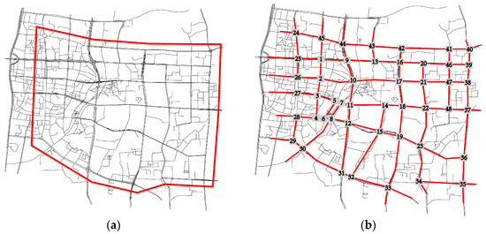
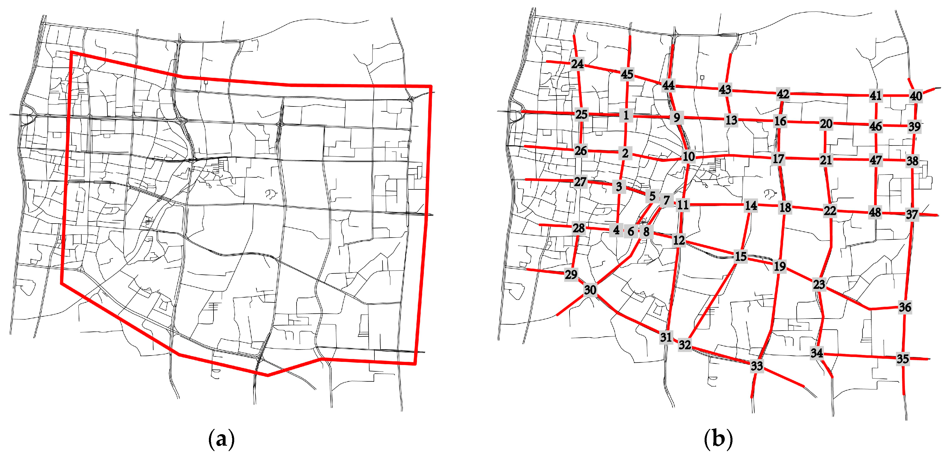
The study area is part of the road network in Changsha City, the scope of which is shown in Figure 5a. The area has an LPR system to collect the information of passing vehicles. According to the location of the data collection points extracted from the LPR system, the road network is transformed into an abstract road network of road sections and intersections, as shown in Figure 5b, which contains 48 intersections.

Figure 5. Study area (a) Scope of road network (b) Abstract road network.

4.2. LPR System Data

The LPR data of Changsha City is obtained from vehicle data collected by fixed collectors. Collectors are usually deployed at key nodes or sections of urban roads. This system utilizes technologies such as high-definition imaging, vehicle detection and image recognition to automatically collect and process the license plate information of passing vehicles. It can conduct round-the-clock uninterrupted monitoring of traffic flow conditions and vehicle behaviors. All LPR data used in this study were fully anonymized prior to analysis. The original license plate numbers were replaced with unique but meaningless identifiers. Therefore, our analysis is entirely based on anonymized vehicle data.

The primary objective of the study is to assess the impact of coordinated control on road network congestion. Therefore, the weekday morning rush hour has been selected as the research subject. During the morning peak hour, traffic congestion on the road network is more pronounced, with some sections experiencing severe congestion. Although the network contains two-way eight-lane roads and two-way ten-lane roads, there are more localized congestion points, which still cause greater traffic pressure on the network. The data set for analysis in the study comprises traffic volumes for five consecutive weekdays from 1 July to 5 July 2019. The LPR data from Changsha show a similar traffic distribution trend across the five weekdays. The selected time period is from 7:00 a.m. to 9:00 a.m. We analyzed traffic volume at 15 min intervals to capture its temporal distribution. The results indicate that traffic demand remained at a high level throughout the 7:00 a.m. to 9:00 a.m. period, rather than peaking sharply at any specific time. Consequently, the averaging method was employed to obtain the morning peak traffic volume. Table 2 presents the base information for the selected intersections.

Table 2. Information of intersection flow.

Number	Direction	Number of Lanes	Traffic Flow (Vehicles/h)	Number	Direction	Number of Lanes	Traffic Flow (Vehicles/h)
2	East	4	1084	12	East	4	838
	West	3	865		West	4	1090
	South	5	765		South	6	1944
	North	6	618		North	6	1104
36	East	/		41	East	5	813
	West	3	602		West	5	892
	South	2	433		South	1	204
	North	2	392		North	/

4.3. Simulation Network

4.3.1. Network Mapping

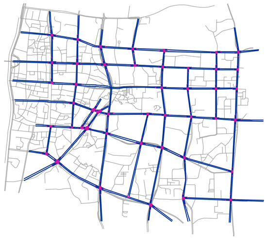
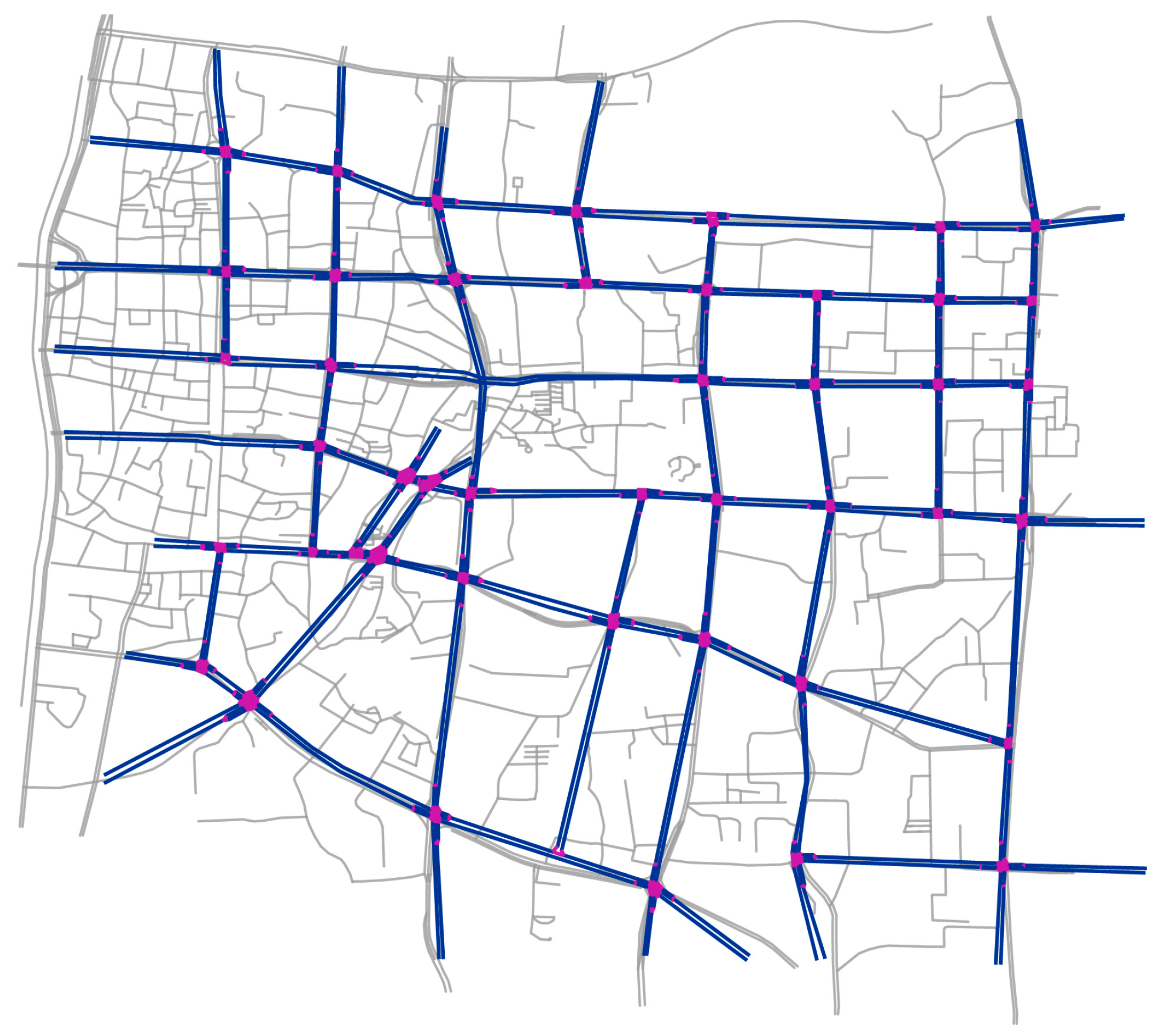
In order to verify the optimization effect, the study requires the construction of a simulated road network. Based on the field survey and the data in the LPR system, the relevant parameters in the abstract road network can be determined, such as the length of the road section, the number of lanes, and the signal timing. The abstract road network is transformed into a simulated road network by these parameters in VISSIM 6.0 software, as shown in Figure 6.

Figure 6. Simulated road network.

It should be noted that the simulated road network does not include all real roads. In the LPR system in Changsha City, there are some intersections where data collection points are not set up, so the roads associated with them are excluded. To reduce the influence of these road flows on the accuracy of the simulated road network, we adjusted the traffic flow load to make the simulation results as close as possible to the real results collected by the LPR system.

4.3.2. Network Calibration

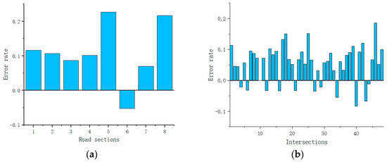
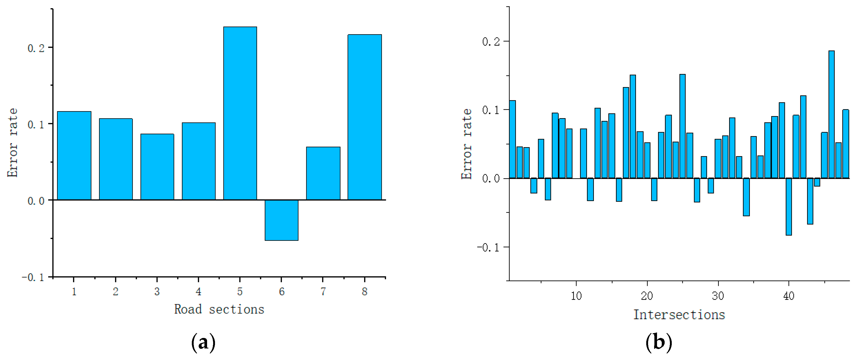
The number of intersections in the study area is high, and using a single indicator to calibrate the road network may have a large error. According to our calculations, calibration using two indicators reduces the error rate by approximately 5% to 12% compared to using a single indicator. Therefore, in the study, we chose to calibrate the data from two indicators, namely the road travel time and the number of vehicles passing the intersection, as shown in Figure 7.

Figure 7. Network calibration (a) Road travel time (b) Number of vehicles passing the intersection.

Firstly, eight road sections were selected from the road network to compare the error rates of the travel times. The maximum error rate is 22%, and the average error rate is 10.9%. In terms of the number of passes, the maximum error rate for the 48 intersections is 18%, and the average error rate is 5.4%. From the results, the simulated road network calibrated with actual data can better simulate the actual operating state and can be used to conduct comparative experiments.

4.4. Network Division and Boundary Control

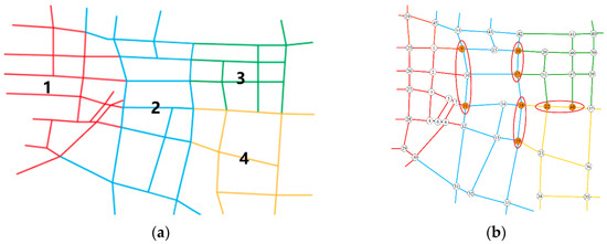
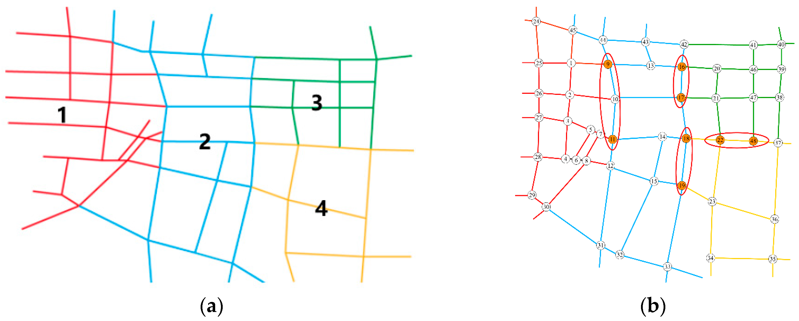
In order to facilitate the control of a large-scale road network, it is necessary to divide the network. In a previous study, we found that dividing the road network into four sub-networks for coordinated control can achieve better results. Therefore, in this study we used the division as a basis for analysis, and the division result is shown in Figure 8a, which employs a normalization algorithm to divide the road network.

Figure 8. Results of road network division and boundary control. (a) Network division. (b) Intersections of boundary control.

Following completion of the sub-network division, flow exchange intersections are established at the sub-network boundary. From the LPR system data of the boundary intersections, the two intersections with the highest traffic volume are identified as flow exchange intersections. The results are presented in Figure 8b.

For the flow exchange, the peak value of the flow within each sub-network is determined by the extreme value of the macro fundamental map fitting. At the conclusion of each control cycle, it is necessary to ascertain the magnitude of the flow of the sub-network in relation to the peak value. The result of the judgment will determine the inflow and outflow of the traffic in the subsequent control cycle.

5. Results and Analysis

In order to ascertain the efficacy of each algorithm in terms of optimization, the study initially compares the optimization effect of the genetic algorithm, particle swarm optimization, and adaptive particle swarm optimization in a simulated road network. Subsequently, chaotic mapping is integrated to address the shortcomings of the particle swarm optimization and to assess its efficacy. In order to enhance the convergence accuracy, a particle swarm optimization incorporating chaotic mapping is employed as a global searcher, while an SQP algorithm is introduced as a local searcher to form an improved chaotic particle swarm optimization. Finally, the chaotic mapping parameters in the improved algorithm are optimized.

To assess the impact of the algorithm on the road network state, a series of indicators are selected, including intersection delay time, intersection saturation, travel time, and the number of stops. Furthermore, the study only coordinates the control of critical paths, so the two cases of areas covered by the critical path and all areas are compared.

5.1. Algorithm Optimization Result

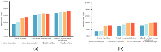
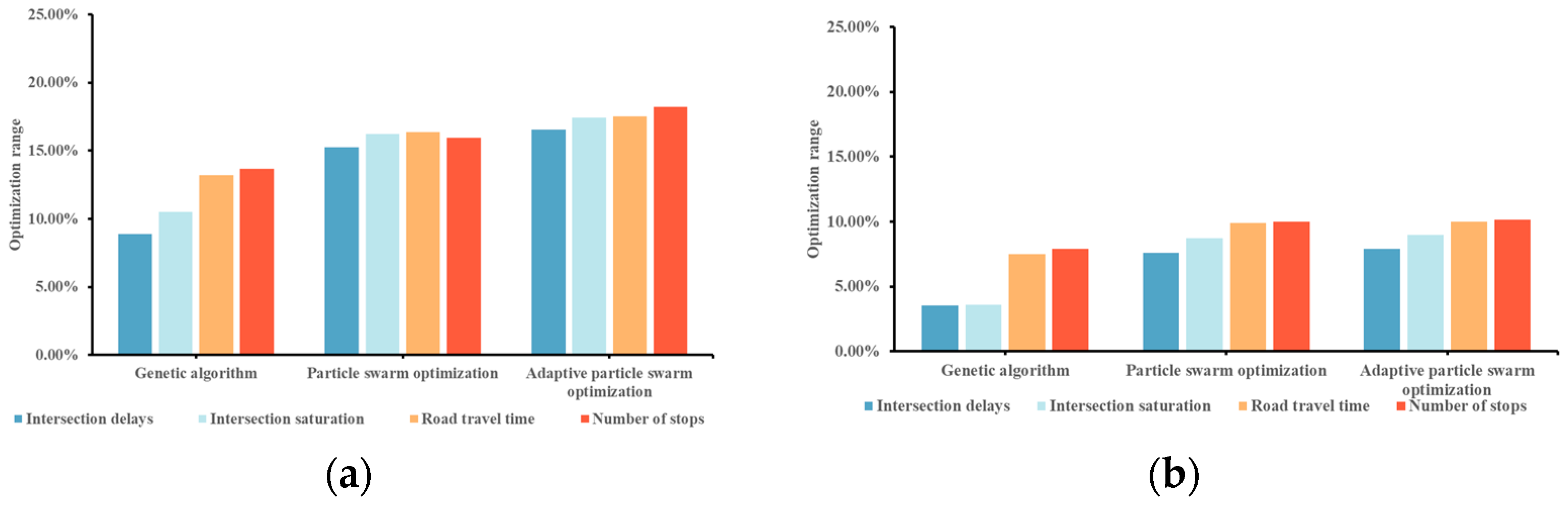
Figure 9 illustrates the optimization of the road network by different algorithms. As the objective of the algorithm is the critical path, the optimization effect of the areas covered by the critical path is considerably higher than that on all areas. Furthermore, the optimization performance of the particle swarm optimization is enhanced by adjusting the particle weights to an adaptive configuration. However, the improvement across all areas is not significant.

Figure 9. Simulation results of algorithms. (a) Areas covered by the critical paths. (b) All areas.

5.2. Results of the Improved Chaotic Particle Swarm Optimization

To address the limitations of particle swarm optimization in global search, the study proposes the incorporation of chaotic mapping as a means of addressing the issue. Chaotic mapping includes a variety of mapping forms. In order to identify the form of chaotic mapping that best matches the current optimization problem, four common chaotic mappings are selected in the study for effect comparison. The results are presented in Table 3 and Table 4. Intersection saturation, defined as the ratio of actual traffic flow to capacity, is a key indicator of traffic congestion. A saturation value close to or exceeding 1.0 indicates that the intersection is operating at or beyond its capacity, leading to increased delays and queue lengths. In this study, saturation is used both as a criterion for identifying network bottlenecks and as a performance metric for evaluating the proposed control strategy.

Table 3. Effect of different chaotic mappings on the optimization rate (areas covered by the critical paths).

	Intersection Delays	Intersection Saturation	Travel Time	Number of Stops
Standard particle swarm	14.52%	15.17%	15.31%	15.84%
Logistic mapping and Particle swarm	17.13%	17.63%	18.01%	18.33%
Tent mapping and Particle swarm	16.98%	17.25%	17.32%	18.01%
Cubic mapping and Particle swarm	16.32%	17.25%	16.85%	17.95%
Sine mapping and Particle swarm	16.63%	17.03%	16.93%	18.005%

Table 4. Effect of different chaotic mappings on the optimization rate (all areas).

	Intersection Delays	Intersection Saturation	Travel Time	Number of Stops
Standard particle swarm	6.49%	7.81%	8.57%	8.75%
Logistic mapping and Particle swarm	8.63%	9.85%	11.01%	10.84%
Tent mapping and Particle swarm	7.93%	9.13%	10.52%	10.33%
Cubic mapping and Particle swarm	7.97%	9.12%	10.17%	10.23%
Sine mapping and Particle swarm	8.01%	9.15%	10.12%	10.28%

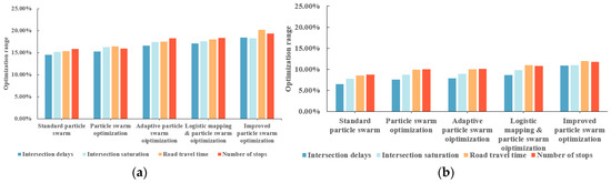
The results show that: (1) The introduction of chaotic mapping to improve the particle swarm optimization algorithm can achieve better optimization results. (2) logistic mapping achieved the best optimization results in all indicators. In areas covered by critical paths, it was able to achieve a rate of over 17%. This indicates that the proposed model achieves a satisfactory optimization effect and meets the requirements of coordinated control. In all areas, it was able to achieve a rate of over 8%. These findings suggest that incorporating logistic mapping into the particle swarm optimization can enhance its performance on the optimization problem. In order to improve the convergence accuracy at the later stage of the algorithm, after incorporating logistic mapping, SQP was introduced as a local search into the particle swarm optimization to obtain the final improved chaotic particle swarm optimization. Figure 10 demonstrates the optimization effect.

Figure 10. Simulation results of improved particle swarm optimization. (a) Areas covered by the critical paths. (b) All areas.

As shown in Figure 10, the optimization effect on the area covered by the critical path is better than that on all areas. This is because the optimization objective is the critical path that is determined through the initial screening. Therefore, after applying the optimization strategy, the improvement effect on the critical path itself is significant. For other sections and areas within the network, their impacts are different. Some sections may benefit from the alleviation of congestion, and the traffic condition improvement is more obvious. Meanwhile, some roads may experience a slight negative impact due to the optimization adjustments, as these adjustments mainly aim to ensure the passage of the critical path. Therefore, in the final effect, the overall performance improvement of the entire network is positive, but compared to the improvement only on the critical path, its effect is not so significant. For large-scale networks, this result is acceptable because the adopted strategy not only improves the performance of the optimization objective but also ensures the efficiency of the entire road network.

5.3. Optimization of Logistic Mapping Parameters

The scale factor in logistic mapping exerts control over the complexity and dynamic behavior of the mapping. If the value is less than 1, the mapping is stable. As the value increases, the dynamic behavior of the mapping becomes increasingly complex, eventually leading to chaos. When the value of the scale factor is greater than 3.57, the mapping enters a chaotic state. As the value continues to increase within the chaotic range (3.57 to 4), the behavior becomes more random and uniformly distributed. At μ = 4, the mapping reaches its fully chaotic state with maximum randomness and the best uniform distribution across the [0, 1] interval, which is ideal for population initialization and perturbation in particle swarm optimization. If the value exceeds 4, the sequence diverges and tends to infinity, making it invalid for optimization. The specific value range depends on the research problem. The study endeavors to optimize the parameters of logistic mapping. Therefore, the optimization encompasses two aspects: the scale factor μ and the population ratio $x_k$.

Several papers have demonstrated that the mapping formulae exhibit chaotic behavior for values of μ taken between 3.6 and 4 [42,43,44]. In order to identify the optimal scale factor for the problem at hand, five alternative values of μ, namely 3.6, 3.7, 3.8, 3.9, and 4.0, were selected at intervals of 0.1 in the study.

For each scale factor, the impact of randomizing the initial position to values within the range of 0 to 1 was evaluated. The optimal initial position at each scale factor was identified based on the optimization results of the phase coordination rate. The results are presented in Table 5.

Table 5. Parameter test results.

μ	${\mathit{x}}_{\mathit{k}}$	Optimal Value of Phase Coordination Rate
3.6	0.3	89.32%
3.7	0.6	88.52%
3.8	0.7	89.63%
3.9	0.6	94.91%
4.0	0.8	95.13%

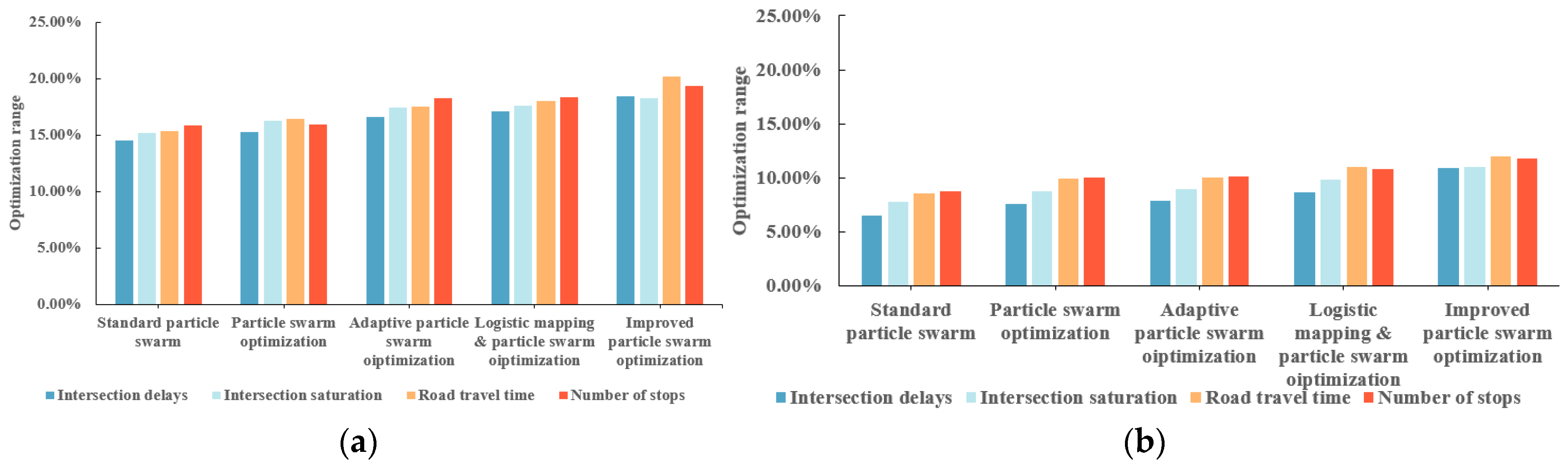
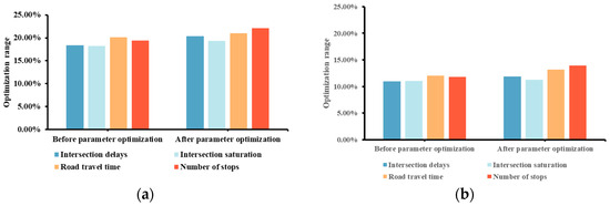
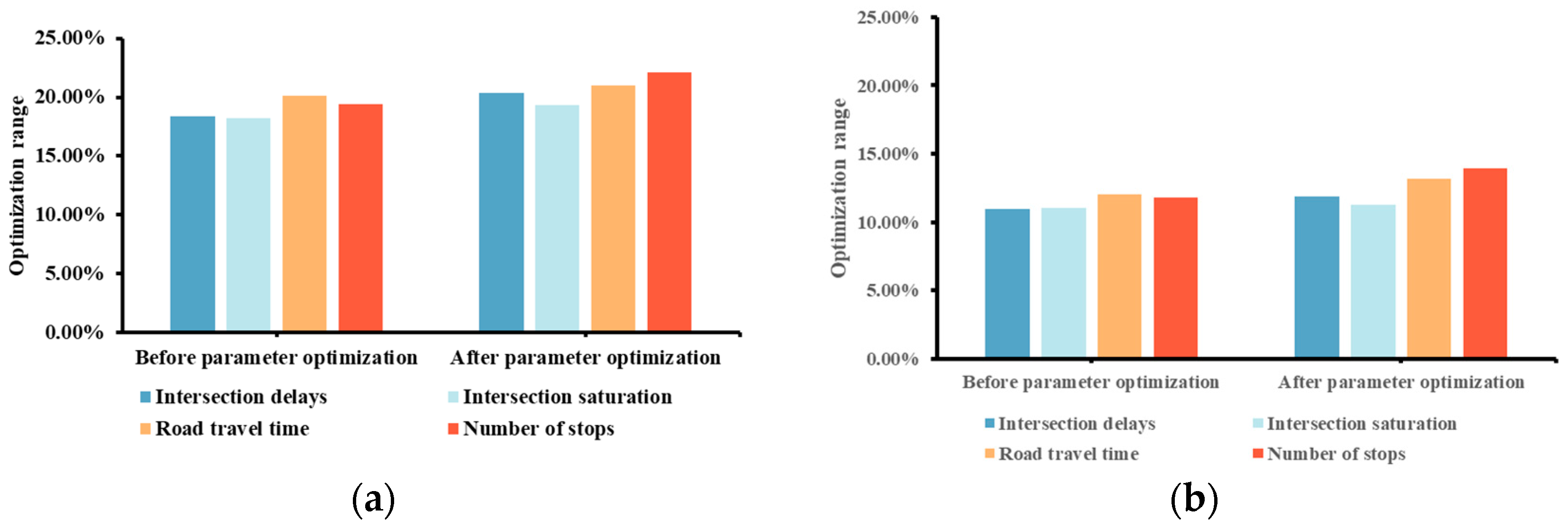
From the results in the table, the best optimization results are obtained when the scale factor is 4.0. Consequently, the logistic mapping with a scale factor of 4.0 and an initial position of 0.8 is integrated into the particle swarm optimization to assess the optimization efficacy. The results are depicted in Figure 11.

Figure 11. Parameter optimization comparison results. (a) Areas covered by the critical paths. (b) All areas.

The results demonstrate that the improved particle swarm optimization based on logistic mapping has achieved superior outcomes in all aspects. In terms of the overall effect of road network improvement, the improved particle swarm optimization achieved better results than the other methods. This shows that the parameter improvement for chaotic mapping makes the model more suitable for the research problem.

5.4. Model Testing

To evaluate the effectiveness of the proposed ICPSO model, we conducted tests from two aspects: validity and stability. Four benchmark functions were selected for the test (Rosenbrock, Sphere, Rastrigin, and Ackley). Each test function was run 30 times independently to ensure statistical significance. The population size was set to 30, and the maximum number of iterations was 500 for all algorithms.

At the same time, we also conducted a Wilcoxon test. This was used to compare the significance of ICPSO compared to the standard PSO. The Wilcoxon signed-rank test was conducted on the optimal values obtained from 30 independent runs for each of the four benchmark functions. The p-values represent the significance test between ICPSO and standard PSO. It should be noted that for the standard PSO to obtain valid results on the four benchmark functions, the search boundaries and convergence criteria were appropriately relaxed. The results are shown in Table 6.

Table 6. Results of model validation and statistical comparison.

Function	Algorithm	Mean ± STD	SR	p-Value
Rosenbrock	PSO	3.83 × 101 ± 1.25 × 101	12%	3.21 × 10−6
	ICPSO	1.80 × 10−3 ± 7.50 × 10−4	96%
Sphere	PSO	6.07 × 10−8 ± 2.12 × 10−8	95%	1.47 × 10−8
	ICPSO	5.67 × 10−15 ± 2.12 × 10−15	97%
Rastrigin	PSO	1.25 × 101 ± 4.32 × 100	72%	2.89 × 10−7
	ICPSO	9.09 × 10−7 ± 3.41 × 10−7	94%
Ackley	PSO	1.86 × 100 ± 5.18 × 10−1	85%	4.53 × 10−6
	ICPSO	1.05 × 10−2 ± 3.78 × 10−3	96%

The results show:

(1)

Model effectiveness: The proposed ICPSO achieves better optimal values and lower mean and standard deviation values compared to PSO across all four benchmark functions. This indicates that the introduction of logistic chaotic mapping and SQP local search effectively enhances the global search capability and convergence accuracy of PSO.

(2)

Model stability: The results demonstrate that ICPSO achieves a higher success rate and lower computational cost, showcasing its superior stability and efficiency.

(3)

Wilcoxon test: All p-values are below the 0.05 significance level, indicating that the differences between ICPSO and PSO are statistically significant. This confirms that the introduction of logistic chaotic mapping and SQP local search leads to a genuine improvement in optimization performance, rather than random variation.

To evaluate the computational cost of the proposed ICPSO, we analyzed its time complexity and compared its runtime with standard PSO. The standard PSO has a time complexity of O(M·N·T), where M is the population size, N is the dimension, and T is the maximum number of iterations. The proposed ICPSO introduces chaotic perturbation and periodic SQP local search. The chaotic perturbation has a complexity of O(M·N·$p_m$·T), where $p_m$ is the chaotic probability (typically 0.1–0.3). The SQP local search has a complexity of O(T·$C_{sqp}$), where $C_{sqp}$ is constant. Since $p_m$ is small and $C_{sqp}$ is constant, the overall complexity remains O(M·N·T), the same order as standard PSO.

A preliminary runtime comparison was conducted on the Rosenbrock function using the same hardware. The average runtime of ICPSO was approximately 1.6 times that of standard PSO (0.83 s vs. 0.52 s over 10 independent runs). Given that the optimization is performed offline and ICPSO achieves significantly better results (as shown in Table 6), this additional computational cost is considered acceptable.

6. Conclusions

In the study, a simulated road network was constructed in VISSIM 6.0 software based on the actual road network. Vehicle data from the LPR system was utilized for calibration. Second, the coordinated control of large-scale road networks is achieved through sub-network division and boundary control. Meanwhile, the path correlation is selected as an indicator to filter the critical paths in the cross-sub-network traffic flow from the vehicle data. In the optimization solution process, the phase coordination rate is taken as the optimization objective. A global searcher is constructed by integrating the improved logistic chaotic mapping and particle swarm optimization, and the sequential quadratic programming search is used as the local searcher. The final stage of the process is the solution of the optimal coordinated control strategy for a multi-sub-network. The effectiveness of the solution is then verified in a simulated road network environment. The main conclusions are as follows:

(1)

The results obtained through the particle swarm optimization can facilitate more effective optimization of the area encompassed by the critical path. However, the improvement in the global road network is limited, and the experimental results also indicate that particle swarm is prone to falling into local optima during the optimization search process.

(2)

The incorporation of chaotic mapping addresses the shortcomings of the particle swarm optimization, and the addition of sequential quadratic programming search further enhances the quality and efficiency of the optimization results. The simulation results of the optimal solution demonstrate improvement in both the critical path coverage area and in all areas. These findings indicate that the improved particle swarm optimization developed in this study can be effectively applied to the coordinated control of large-scale urban road networks.

(3)

Optimizing the initial position and scale factor of the logistic mapping can improve the control effect. The coordinated control model proposed achieves a phase coordination rate indicator of 95.13%. Concurrently, other traffic indicators such as intersection saturation, intersection delay time, road section travel time, and the average number of stops are also improved. This demonstrates that parameter optimization can further improve the algorithm’s effectiveness for this problem.

The coordinated control model proposed targets the critical paths in the cross-sub-network flows, and therefore the coordinated control optimizes only the intersections and road sections covered by a part of the paths. For other road sections and intersections, the coordination scheme also has a positive effect on most of them. However, some road sections will have slight negative effects due to vehicle detours and signal changes. It should be noted that the study has not yet considered the contingency factors that exist in the real road environment. Consequently, the optimization effect of coordinated control on the road network may be lower than the experimental effect in practical applications.

References

- Robertson, D.I.; Bretherton, R.D. Optimum control of an intersection for any known sequence of vehicle arrivals. In Proceedings of the 2nd IFAC/IFIP/IFORS Symposium on Traffic Control and Transportation Systems, Monte Carlo, Monaco, 16–21 September 1974. [Google Scholar]
- Shelby, S.G. Single-intersection evaluation of real-time adaptive traffic signal control algorithms. Transp. Res. Rec. 2004, 1867, 183–192. [Google Scholar] [CrossRef] [Scilit]
- Guler, S.I.; Cassidy, M.J. Strategies for sharing bottleneck capacity among buses and cars. Transp. Res. Part B Methodol. 2012, 46, 1334–1345. [Google Scholar] [CrossRef] [Scilit]
- Gayah, V.V.; Daganzo, C.F. Analytical capacity comparison of one-way and two-way signalized street networks. Transp. Res. Rec. 2012, 2301, 76–85. [Google Scholar] [CrossRef] [Scilit]
- Ji, Y.; Geroliminis, N. On the spatial partitioning of urban transportation networks. Transp. Res. Part B Methodol. 2012, 46, 1639–1656. [Google Scholar] [CrossRef] [Scilit]
- Saeedmanesh, M.; Geroliminis, N. Clustering of heterogeneous networks with directional flows based on “snake” similarities. Transp. Res. Part B. Methodol. 2016, 91, 1146–1165. [Google Scholar] [CrossRef] [Scilit]
- Lopez, C.; Leclercq, L.; Krishnakumari, P.; Chiabaut, N.; Lint, H.V. Revealing the day-to-day regularity of urban congestion patterns with 3d speed maps. Sci. Rep. 2017, 7, 14029. [Google Scholar] [CrossRef] [Scilit]
- Lukas Ambühl Loder, A.; Zheng, N.; Axhausen, K.W.; Menendez, M. Approximative network partitioning for MFDs from stationary sensor data. Transp. Res. Rec. 2019, 2673, 94–103. [Google Scholar] [CrossRef] [Scilit]
- Yang, S.; Wu, J.; Xu, Y.; Yang, T. Revealing heterogeneous spatiotemporal traffic flow patterns of urban road network via tensor decomposition-based clustering approach. Phys. A Stat. Mech. Its Appl. 2019, 526, 121086. [Google Scholar] [CrossRef] [Scilit]
- Hu, Y.; Wang, Y.; Zhang, J.; Yu, H. Correlation degree analysis of arterial adjacent intersections for coordinated control subunit partition. Adv. Mech. Eng. 2018, 10, 1687814017748748. [Google Scholar] [CrossRef] [Scilit]
- Dimitriou, L.; Lentzakis, A.F.; Nikolaos, G. Dynamic partitioning of urban road networks based on their topological and operational characteristics. In Proceedings of the 2017 5th IEEE International Conference on Models and Technologies for Intelligent Transportation Systems (MT-ITS), Naples, Italy, 26–28 June 2017; Volume 59, pp. 457–462. [Google Scholar] [CrossRef] [Scilit]
- Niu, X.; Zhu, J.; Wu, C.Q.; Wang, S. On a clustering-based mining approach for spatially and temporally integrated traffic sub-area division. Eng. Appl. Artif. Intell. 2020, 96, 103932. [Google Scholar] [CrossRef] [Scilit]
- Wen, L.; Dong, B.; Li, P.; Yan, A. Signal coordination control based on comprehensive correlation degree. IOP Conf. Ser. Earth Environ. Sci. 2021, 638, 012030. [Google Scholar] [CrossRef] [Scilit]
- Aboudolas, K.; Papageorgiou, M.; Kouvelas, A.; Kosmatopoulos, E.B. A rolling-horizon quadratic-programming approach to the signal control problem in large-scale congested urban road networks. Transp. Res. Part C Emerg. Technol. 2010, 18, 559–576. [Google Scholar] [CrossRef] [Scilit]
- de Oliveira, L.B.; Camponogara, E. Predictive control for urban traffic networks: Initial evaluation. IFAC Proc. Vol. 2007, 40, 424–429. [Google Scholar] [CrossRef] [Scilit]
- Hajbabaie, A.; Benekohal, R.F. A program for simultaneous network signal timing optimization and traffic assignment. IEEE Trans. Intell. Transp. Syst. 2015, 16, 2573–2586. [Google Scholar] [CrossRef] [Scilit]
- Feng, Y.H.; Head, K.L.; Khoshmagham, S.; Zamanipour, M. A real-time adaptive signal control in a connected vehicle environment. Transp. Res. Part C Emerg. Technol. 2015, 55, 460–473. [Google Scholar] [CrossRef] [Scilit]
- Huang, W.; Hu, J.; Huang, G.Y.; Lo, H.K. A three-layer hierarchical model-based approach for network-wide traffic signal control. Transp. B Transp. Dyn. 2023, 11, 1912–1942. [Google Scholar] [CrossRef] [Scilit]
- Wang, W.; Zhang, H.; Qiao, T.; Ma, J.; Jin, J.; Wu, W.; Jiang, Y. Real-Time Network-Level Traffic Signal Control: An Explicit Multiagent Coordination Method. IEEE Trans. Intell. Transp. Syst. 2024, 25, 19688–19698. [Google Scholar] [CrossRef] [Scilit]
- Zhang, Y.; Goel, H.; Li, P.; Damani, M.; Chinchali, S.; Sartoretti, G. Coordlight: Learning decentralized coordination for network-wide traffic signal control. IEEE Trans. Intell. Transp. Syst. 2025, 26, 8034–8049. [Google Scholar] [CrossRef] [Scilit]
- Chuo, H.S.E.; Tan, M.K.; Chong, A.C.H.; Chin, R.K.Y.; Teo, K.T.K. Evolvable traffic signal control for intersection congestion alleviation with enhanced particle swarm optimization. In Proceedings of the 2017 IEEE 2nd International Conference on Automatic Control and Intelligent Systems, Kota Kinabalu, Malaysia, 21 October 2017. [Google Scholar] [CrossRef] [Scilit]
- Shi, Y.; Qi, Y.; Lv, L.; Liang, D. A particle swarm optimisation with linearly decreasing weight for real-time traffic signal control. Machines 2021, 9, 280. [Google Scholar] [CrossRef] [Scilit]
- Okulewicz, M.; Mańdziuk, J. The impact of particular components of the PSO-based algorithm solving the dynamic vehicle routing problem. Appl. Soft Comput. 2017, 58, 586–604. [Google Scholar] [CrossRef] [Scilit]
- Yelure, B.; Sonavane, S. Particle swarm optimization based routing method for vehicular ad-hoc network. In Proceedings of the 2020 International Conference on Communication and Signal Processing (ICCSP), Chennai, India, 28–30 July 2020. [Google Scholar] [CrossRef] [Scilit]
- Hatri, A.; Bouabdellah, A.; Boumhidi, J. Q-learning based intelligent multi-objective particle swarm optimization of light control for traffic urban congestion management. Int. J. Intell. Eng. Inform. 2016, 4, 327–344. [Google Scholar] [CrossRef] [Scilit]
- Li, D.; Ranjitkar, P.; Zhao, Y. Mitigating recurrent congestion via particle swarm optimization variable speed limit controllers. KSCE J. Civ. Eng. 2019, 23, 3174–3179. [Google Scholar] [CrossRef] [Scilit]
- Garcia-Nieto, J.; Olivera, A.C.; Alba, E. Optimal cycle program of traffic lights with particle swarm optimization. IEEE Trans. Evol. Comput. 2013, 17, 823–839. [Google Scholar] [CrossRef] [Scilit]
- El Hatri, C.; Boumhidi, J. Traffic management model for vehicle re-routing and traffic light control based on Multi-Objective Particle Swarm Optimization. Intell. Decis. Technol. 2017, 11, 199–208. [Google Scholar] [CrossRef] [Scilit]
- Zhang, Y.; Ni, Q. A coordinated traffic control on urban expressways with modified particle swarm optimization. KSCE J. Civ. Eng. 2017, 21, 501–511. [Google Scholar] [CrossRef] [Scilit]
- Qin, H.; Zhang, W.; Zhai, H. Cooperative control of multiple intersections combining agent and chaotic particle swarm optimization. Comput. Electr. Eng. 2023, 110, 108875. [Google Scholar] [CrossRef] [Scilit]
- Olivera, A.C.; Vidal, P.J. A multi-objective swarm approach with pedestrians spotlight in traffic urban optimisation. IEEE Lat. Am. Trans. 2022, 20, 2363–2370. [Google Scholar] [CrossRef] [Scilit]
- Yuen, M.C.; Ng, S.C.; Leung, M.F. A competitive mechanism multi-objective particle swarm optimization algorithm and its application to signalized traffic problem. Cybern. Syst. 2020, 52, 73–104. [Google Scholar] [CrossRef] [Scilit]
- Yong, Z.; Peng, W. Optimal control for region of the city traffic signal based on selective particle swarm optimization algorithm. In Proceedings of the 2015 International Conference on Intelligent Transportation, Big Data and Smart City, Halong Bay, Vietnam, 19–20 December 2015. [Google Scholar] [CrossRef] [Scilit]
- Subrahmanyam, V.; Nagesh, O.S.; Reddy, Y.V.; Rao, A.P.; Suresh, M.; Neelima, G. Internet of Things (IoT) Enabled Intelligent Traffic Control Management System By Hybrid Swarm Intelligence (SI) Algorithm. In Proceedings of the 2024 IEEE International Conference on Interdisciplinary Approaches in Technology and Management for Social Innovation (IATMSI), Gwalior, India, 14–16 March 2024. [Google Scholar] [CrossRef] [Scilit]
- Lin, Z.; Gao, K.; Wu, N.; Suganthan, P.N. Problem-Specific Knowledge Based Multi-Objective Meta-Heuristics Combined Q-Learning for Scheduling Urban Traffic Lights with Carbon Emissions. IEEE Trans. Intell. Transp. Syst. 2024, 25, 15053–15064. [Google Scholar] [CrossRef] [Scilit]
- Ma, C.; Yu, C.; Zhang, C.; Yang, X. Signal timing at an isolated intersection under mixed traffic environment with self-organizing connected and automated vehicles. Comput.-Aided Civ. Infrastruct. Eng. 2023, 38, 1955–1972. [Google Scholar] [CrossRef] [Scilit]
- Konishi, K.; Kokame, H.; Hirata, K. Coupled map car-following model and its delayed-feedback control. Phys. Rev. E 1999, 60, 4004–4009. [Google Scholar] [CrossRef] [Scilit]
- Dong, C.; Liu, Z.; Qiu, Z. Urban traffic signal timing optimization based on multi-layer chaos neural networks involving feedback. In Proceedings of the Advances in Natural Computation: First International Conference, Changsha, China, 27–29 August 2005. [Google Scholar] [CrossRef] [Scilit]
- Zhao, X.; Gao, Z. A control method for congested traffic induced by bottlenecks in the coupled map car-following model. Phys. A Stat. Mech. Its Appl. 2006, 366, 513–522. [Google Scholar] [CrossRef] [Scilit]
- Narh, A.T.; Thorpe, N.; Bell, M.C.; Hill, G.A. Do new sources of traffic data make the application of Chaos Theory to traffic management a realistic possibility? Transp. Rev. 2016, 36, 635–658. [Google Scholar] [CrossRef] [Scilit]
- Zhong, J.Q.; Zhang, M.T.; Tan, J.J. RBF neural network-based adaptive control for Aw–Rascle–Zhang mixed traffic flow model with unknown external disturbances. Phys. A Stat. Mech. Its Appl. 2026, 681, 131074. [Google Scholar] [CrossRef] [Scilit]
- Phatak, S.C.; Rao, S.S. Logistic map: A possible random-number generator. Phys. Rev. E 1995, 51, 3670. [Google Scholar] [CrossRef] [Scilit] [PubMed]
- Chen, S.; Feng, S.; Fu, W.; Zhang, Y. Logistic map: Stability and entrance to chaos. J. Phys. Conf. Ser. 2021, 2014, 012009. [Google Scholar] [CrossRef] [Scilit]
- Xiang, H.; Liu, L. An improved digital logistic map and its application in image encryption. Multimed. Tools Appl. 2020, 79, 30329–30355. [Google Scholar] [CrossRef] [Scilit]
Disclaimer/Publisher’s Note: The statements, opinions and data contained in all publications are solely those of the individual author(s) and contributor(s) and not of MDPI and/or the editor(s). MDPI and/or the editor(s) disclaim responsibility for any injury to people or property resulting from any ideas, methods, instructions or products referred to in the content. |
© 2026 by the authors. Licensee MDPI, Basel, Switzerland. This article is an open access article distributed under the terms and conditions of the Creative Commons Attribution (CC BY) license.