The q-Deformed Lindley Distribution: Properties, Statistical Inference, and Applications

Abstract

This paper introduces a q-deformed extension of the Lindley distribution. This extension is obtained by replacing the classical exponential with the q-exponential function from Tsallis non-extensive statistical techniques. This transformation offers more control over the tail behavior of the distribution, providing a transition between exponential and power-law decay patterns. Such flexibility is particularly useful when modeling right-skewed data with excess kurtosis, where classical models may not adequately describe heavy-tailed and highly skewed data. We derive several key properties, including the quantile function, expressed by the Lambert–Tsallis function Wq, the raw and incomplete moments, the probability-weighted moments, and the Tsallis entropy. The distribution of order statistics is also investigated. For parameter estimation, we employ several frequentist methods and conduct extensive Monte Carlo simulation studies to assess and compare their performance. Finally, applications to real-world datasets show that the q-deformed Lindley model is practically superior and more flexible than the classical Lindley distribution and other well-known models.

1. Introduction

Lifetime distributions are essential in reliability engineering, survival analysis, actuarial science, and many other applied fields, where it is important to achieve an appropriate balance between modeling flexibility and analytical tractability. Among classical one-parameter lifetime models, the Lindley distribution, originally introduced by Lindley [1], has attracted considerable attention from researchers and practitioners due to its ability to provide a better fit for lifetime data than the exponential distribution in many practical situations. Moreover, its simple analytical structure and the availability of closed-form expressions for several statistical properties further enhance its usefulness. These characteristics have facilitated both theoretical developments and practical applications; see, for example, ref. [2]. The probability density function (PDF) and the cumulative distribution function (CDF) of the Lindley distribution are

$$g(x;\theta )={\displaystyle \frac{{\theta }^2}{1+\theta }}(1+x)e^{-\theta x},x>0,\theta >0,$$

(1)

and

$$G(x;\theta )=1-\left(1+{\displaystyle \frac{\theta x}{1+\theta }}\right)e^{-\theta x},$$

(2)

respectively. Several extensions of the Lindley distribution have been proposed and studied in the literature. Early contributions include the generalized Lindley distribution [3,4], the extended Lindley distribution and its zero-truncated version [5]. Additional shape flexibility was introduced through the two-parameter weighted Lindley distribution [6] and the power Lindley distribution [7]. Several further modifications have also been proposed, including the quasi-Lindley distribution [8], transmuted Lindley distribution [9], alpha-power transformed Lindley distribution [10], the new weighted Lindley distribution [11], the Lindley distribution with a location parameter [12], the modified Lindley distribution [13], the Rayleigh–Lindley distribution [14], and the Lindley-exponential distribution [15]. The Lindley family of distributions was proposed by [16]. Authors also proposed the odd Lindley-G family of distributions [17] and its special case, the two-parameter odd Lindley Weibull distribution [18]. More recent contributions include the compound exponentiated power Lindley power series distribution [19]. The q-Lindley distribution was proposed as a one-parameter lifetime model constructed within the exponential family [20]. The Lindley q-distribution was proposed by [21] as a q-analogue of the Lindley model within the framework of the Jackson q-calculus, focusing on the q-theoretic characteristics. In addition to these models, numerous other Lindley-type distributions have been proposed in the literature.

On the other hand, extensions of the classical exponential and logarithmic functions arise from the framework of non-extensive statistical mechanics introduced by Tsallis [22], where the classical Boltzmann–Gibbs entropy is generalized into a non-extensive entropy measure indexed by a deformation parameter q. The q-exponential and q-logarithmic functions are defined as

$${\log }_q\left(x\right)={\displaystyle \frac{x^{1-q}-1}{1-q}},{\exp }_q\left(x\right)={\left[1+(1-q)x\right]}^{\frac{1}{1-q}},\mathrm{if}1+(1-q)x>0.$$

As $q\to 1$, these expressions recover the standard natural logarithm and exponential functions.

Recently, several q-deformation statistical distributions have been developed using the pathway model proposed by [23]. In particular, the pathway formulation reduces to the Tsallis-type q-exponential as a special case and provides a framework for constructing probability models derived from non-extensive entropy principles [24]. Within this context, a broad class of q-deformed distributions has been proposed, including the q-exponential and q-Weibull distributions [25,26], the q-logistic family [27], the q-Gaussian distribution [28], the q-extended inverse Gaussian distribution [29], the q-Nakagami distribution [30], the q-Pareto distribution [31], as well as q-generalized extreme value and q-Gumbel distributions [32,33]. Recent developments also include Tsallis log-scale-location models [34], which facilitate the study of moments, stochastic ordering, and the Gini index within a deformed context.

Although the Lindley distribution is valued for its simplicity and reliability in lifetime data analysis, its fixed exponential component may restrict its ability to capture diverse tail behaviors and varying distributional shapes observed in complex real-world phenomena. To address this limitation, this paper proposes a q-deformed extension of the Lindley distribution by replacing the exponential term $e^{-\theta x}$ in the classical density with the q-exponential function ${\exp }_q(-\theta x)$. Although several analytical steps rely on known properties of the q-exponential function, the contribution of this work lies in showing how these tools lead to a tractable and practically useful q-deformed extension of the Lindley distribution, together with its inferential development and empirical validation. This formulation offers more flexibility while maintaining mathematical tractability. The proposed model preserves the classical Lindley distribution as a limiting case when $q\to 1$, while introducing an additional deformation parameter that allows enhanced control over the behavior of the tail and the support properties.

The main contributions of this paper are as follows: In Section 2, the q-deformed Lindley distribution is proposed. Section 3 investigates several properties of the proposed distribution. In Section 4, statistical inference for the q-deformed Lindley distribution is developed. Monte Carlo simulation studies are carried out in Section 5 to assess the performance of the proposed estimators under different parameter configurations. Section 6 presents applications to real datasets to demonstrate the practical usefulness of the proposed distribution and to compare its performance with several well-known lifetime models.

2. The q-Deformed Lindley Distribution

The q-deformed Lindley (qDL) distribution is obtained by replacing the exponential term in the Lindley distribution with the q-exponential function

$${\exp }_q(-\theta x)=\left\{\begin{array}{cc}{\left[1-(1-q)\theta x\right]}^{\frac{1}{1-q}},\hfill & 1-(1-q)\theta x>0,\hfill \\ 0,\hfill & \mathrm{otherwise},\hfill \end{array}\right.$$

(3)

where $\theta >0$ and $q\ne 1$. This modification introduces an additional parameter q that directly affects the tail behavior and distribution support, allowing for greater flexibility in modeling skewed and heavy-tailed data. The following proposition provides the explicit form of the PDF of the qDL distribution.

Proposition 1. 

The probability density function of the q-deformed Lindley is given by

$$f(x;\theta ,q)={\displaystyle \frac{(2-q)(3-2q){\theta }^2}{1+(3-2q)\theta }}(1+x){\exp }_q(-\theta x),\theta >0,$$

(4)

with support

$$x\in \left\{\begin{array}{cc}(0,\infty )\hfill & if1<q<3/2\hfill \\ (0,{\displaystyle \frac{1}{(1-q)\theta }})\hfill & ifq<1\hfill \end{array}\right.$$

Proof. 

The PDF of the qDL distribution is obtained by replacing the exponential term in the Lindley distribution (1) with the q-exponential function (3). This yields the kernel

$$f(x;\theta ,q)=C(\theta ,q)(1+x){\exp }_q(-\theta x),$$

where $C(\theta ,q)$ is a normalizing constant

$$C(\theta ,q)={\displaystyle \frac{1}{Z_q}},Z_q={\int }_0^{\infty }(1+x){\exp }_q(-\theta x)dx.$$

To evaluate $Z_q$, Lemma 1 of Zhang et al. [35] is useful, since it generalizes the gamma and incomplete gamma integrals for the q-exponential function:

$${\int }_0^{\infty }{x}^{\alpha }{\exp }_q(-\theta x)dx={\displaystyle \frac{\mathrm{\Gamma }(\alpha +1)}{{\theta }^{\alpha +1}{\phi }_q(\alpha +1)}},$$

(5)

where, ${\phi }_q\left(\alpha \right)=(2-q)(3-2q)\cdots (\alpha +1-\alpha q),{\phi }_q\left(0\right)=1$. Applying this with $\alpha =0$ and $\alpha =1$, we obtain

$$Z_q={\displaystyle \frac{1}{\theta (2-q)}}+{\displaystyle \frac{1}{{\theta }^2(2-q)(3-2q)}}={\displaystyle \frac{1+(3-2q)\theta }{{\theta }^2(2-q)(3-2q)}},$$

and therefore

$$C(\theta ,q)={\displaystyle \frac{(2-q)(3-2q){\theta }^2}{1+(3-2q)\theta }}.$$

Zhang et al. [35] present the condition $q\in (0,1+1/\alpha )$ for convergence of these integrals. Although this is sufficient for formal derivations, a sharper restriction is obtained from the asymptotic behavior of the q-exponential. For $q>1$,

$${\exp }_q(-\theta x)\sim {\left[(q-1)\theta x\right]}^{-1/(q-1)}\mathrm{as}x\to \infty ,$$

which implies

$$x^{\alpha }{\exp }_q(-\theta x)\sim x^{\alpha -\frac{1}{q-1}}.$$

The integral ${\int }_0^{\infty }{x}^{\alpha }{\exp }_q(-\theta x)dx$ converges only if $\alpha -\frac{1}{q-1}<-1$, i.e.,

$$q<1+{\displaystyle \frac{1}{\alpha +1}}.$$

In particular, for $\alpha =0$, convergence requires $q<2$, while for $\alpha =1$, convergence requires $q<1.5$. Therefore, the qDL distribution is well defined for $q<1$ (bounded support with $0<x<1/\left(\right(1-q\left)\theta \right)$) and for $1<q<1.5$ (infinite support on $(0,\infty )$). For $q\ge 3/2$, the normalizing constant diverges, and the distribution is not defined.    □

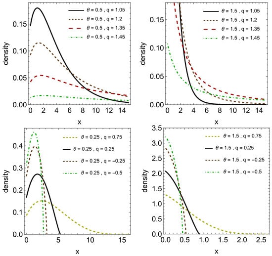
The PDF of the qDL distribution is presented in Figure 1 for selected values of $\theta$ and q. The distribution is right-skewed, and the parameter q controls the degree of skewness and tail thickness. For $1<q<3/2$, the support is unbounded and the PDF exhibits heavy, power-law tail behavior, and increasing q leads to heavier right tails. In contrast, when $q<1$, the support becomes finite, and the PDF drops sharply to zero at the upper bound. As $q\to 1$, we recover the standard Lindley distribution. The CDF corresponding to (4) is formally established in the following proposition.

Figure 1. PDF of the qDL distribution for selected values of $\theta$ and q.

Proposition 2. 

The cumulative distribution function of the q-deformed Lindley distribution is given by

$$F(x;\theta ,q)=1-\left[1+{\displaystyle \frac{(2-q)\theta x}{1+(3-2q)\theta }}\right]{({\exp }_q(-\theta x))}^{2-q},\theta >0$$

(6)

with support

$$x\in \left\{\begin{array}{cc}(0,\infty )\hfill & if1<q<3/2\hfill \\ \left(0,{\displaystyle \frac{1}{(1-q)\theta }}\right)\hfill & ifq<1\hfill \end{array}\right.$$

Proof. 

By definition, the CDF of the qDL distribution is given by

$$\begin{array}{ccc}\hfill F(x;\theta ,q)& =& {\int }_0^{x}f(t;\theta ,q)dt.\hfill \\ & =& {\displaystyle \frac{(2-q)(3-2q){\theta }^2}{1+(3-2q)\theta }}{\int }_0^x(1+t){\exp }_q(-\theta t)dt.\hfill \end{array}$$

Using Lemma 1 of Zhang et al. [35], we have

$${\int }_0^x{t}^{\alpha }{\exp }_q(-\theta t)dt={\displaystyle \frac{\mathrm{\Gamma }(\alpha +1)}{{\theta }^{\alpha +1}{\phi }_q(\alpha +1)}}\left\{1-\sum _{k=0}^{\alpha }{\displaystyle \frac{{\left(\theta x\right)}^k}{k!}}{\displaystyle \frac{{\phi }_q(\alpha +1)}{{\phi }_q(\alpha +1-k)}}{\left[{\exp }_q(-\theta x)\right]}^{{\displaystyle \frac{{\phi }_q(\alpha -k+1)}{{\phi }_q(\alpha -k)}}}\right\}.$$

(7)

Applying this result to $\alpha =0$ and $\alpha =1$, we obtain

$$F(x;\theta ,q)=1-{\displaystyle \frac{{({\exp }_q(-\theta x))}^{3-2q}+\theta (3-2q)(1+x){({\exp }_q(-\theta x))}^{2-q}}{1+(3-2q)\theta }}.$$

In a simpler form, the CDF for the qDL distribution is given by (6).    □

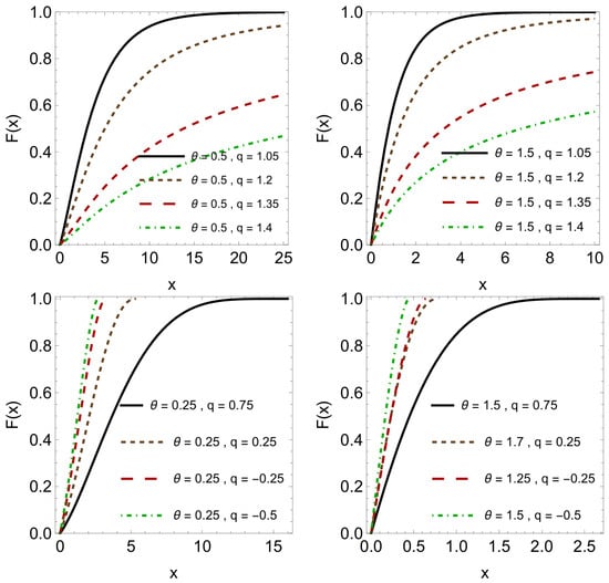
It is straightforward to verify that $F\left(0\right)=0$ and $F\left(x\right)\to 1$ as $x\to \infty$ (for $1<q<3/2$) or $x\to 1/{\left((1-q)\theta \right)}^{-}$ (for $q<1$). The cumulative distribution function has been plotted for several choices of the parameters $\theta$ and q in the admissible ranges $q<1$ and $1<q<3/2$; see Figure 2. Since the support of the distribution depends on q, separate plots are produced for the bounded-support case $q<1$ and the unbounded-support case $1<q<3/2$. The plots confirm that the CDF is increasing monotonically from 0 to 1, and illustrate the effect of the parameters on the rate of accumulation of the probability mass.

Figure 2. CDF of the qDL distribution for selected values of $\theta$ and q.

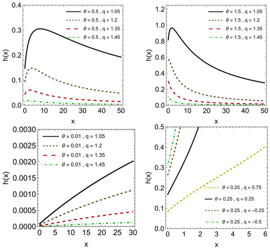
The Hazard rate function of the qDL distribution is given by

$$h(x;\theta ,q)={\displaystyle \frac{(2-q)(3-2q){\theta }^2}{1+(3-2q)\theta +(2-q)\theta x}}(1+x){\left[1-(1-q)\theta x\right]}^{-1},\theta >0$$

(8)

with support

$$x\in \left\{\begin{array}{cc}(0,\infty )\hfill & \mathrm{if}1<q<3/2\hfill \\ \left(0,{\displaystyle \frac{1}{(1-q)\theta }}\right)\hfill & \mathrm{if}q<1\hfill \end{array}\right.$$

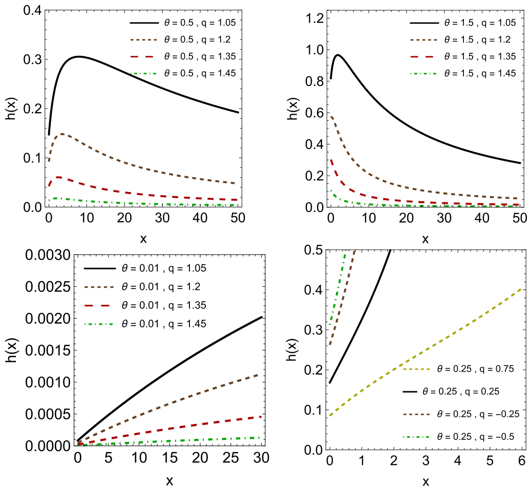
Figure 3 shows that the hazard rate of the qDL distribution can be increasing or unimodal.

Figure 3. Hazard rate function of the qDL distribution for selected values of $\theta$ and q.

To clarify the identifiability of the parameters, consider two pairs of parameters $({\theta }_1,q_1)$ and $({\theta }_2,q_2)$ such that $f(x;{\theta }_1,q_1)=f(x;{\theta }_2,q_2).$ In the bounded-support case ($q<1$), the support endpoint $x_{max}={\displaystyle \frac{1}{(1-q)\theta }}$ is uniquely determined by $(\theta ,q)$. Hence, equality of the supports implies $(1-q_1){\theta }_1=(1-q_2){\theta }_2.$ Additionally, the exponent $1/(1-q)$ governing the decay near the boundary uniquely determines q, which in turn identifies $\theta$ through the endpoint relation.

In the unbounded-support case ($1<q<3/2$), the tail behavior satisfies $f\left(x\right)\sim x^{-{\displaystyle \frac{1}{q-1}}}\mathrm{as}x\to \infty ,$ so the tail index uniquely determines q. Once q is fixed, the scale parameter $\theta$ can be identified from the normalization constant or from the hazard rate expression.

Therefore, the parameter pair $(\theta ,q)$ is structurally identifiable over the admissible parameter space. However, when $q\to 1$, the model approaches the classical Lindley distribution, and the influence of q diminishes, leading to weaker practical identifiability and potential instability in estimation.

3. Properties

3.1. Quantile Function

The quantile function of the qDL distribution can be obtained via Lambert–Tsallis $W_q$ function introduced by [36] as a q-generalization of the Lambert W function to solve the equation $W_q\left(z\right){\exp }_q^z=z$.

Theorem 1. 

For $u\in (0,1)$, the quantile function, $Q\left(u\right)=F^{-1}\left(u\right)$, of the qDL distribution is defined by

$$Q(u;\theta ,q)=-{\displaystyle \frac{A+\kappa W_{q^{\prime }}\left(-\frac{A(1-u)}{\kappa {\exp }_{q^{\prime }}\left(A\right)}\right)}{(2-q)\theta }},$$

(9)

where $A=1+(3-2q)$, $q^{\prime }={\displaystyle \frac{1}{2-q}}$, $\kappa =1+(1-q^{\prime })A$ and $W_q(·)$ denote the Lambert–Tsallis function. To obtain $Q\left(u\right)>0$, use the real lower branch of $W_{q^{\prime }}$.

Proof. 

Write CDF (6) as

$$1-u={\displaystyle \frac{A+(2-q)\theta x}{A}}{({\exp }_q(-\theta x))}^{2-q}.$$

Let $z=-(2-q)\theta x$ and using the following relation from [37]:

$${({\exp }_q(-\theta x))}^{2-q}={\exp }_{q^{\prime }}\left(z\right)\mathrm{where}{q}^{\prime }={\displaystyle \frac{1}{2-q}},$$

we obtain

$$(z-A){\exp }_{q^{\prime }}\left(z\right)=-(1-u)A.$$

Divide by ${\exp }_{q^{\prime }}\left(A\right)$ and use the $q^{\prime }$-subtraction identity

$${\displaystyle \frac{{\exp }_{q^{\prime }}\left(z\right)}{{\exp }_{q^{\prime }}\left(A\right)}}={exp}_{q^{\prime }}\left(z-{}_{q\prime }A\right),$$

where $z-{}_{q\prime }A={\displaystyle \frac{z-A}{1+(1-q^{\prime })A}}$; we obtain:

$$(z-A){\exp }_{q^{\prime }}(z-{}_{q\prime }A)=-{\displaystyle \frac{(1-u)A}{{\exp }_{q^{\prime }}\left(A\right)}}.$$

Divide both sides by $\kappa =1+(1-q^{\prime })A$ and the last equation becomes

$$(z-{}_{q\prime }A){\exp }_{q^{\prime }}(z-{}_{q\prime }A)=-{\displaystyle \frac{(1-u)A}{{\exp }_{q^{\prime }}\left(A\right)}}.$$

By the definition of the Lambert–Tsallis function

$$z-{}_{q\prime }A=W_{q^{\prime }}\left(-{\displaystyle \frac{A(1-u)}{\kappa e_{q^{\prime }}\left(A\right)}}\right).$$

After some algebra, we obtain the quantile function of the qDL distribution as

$$Q(u;\theta ,q)=-{\displaystyle \frac{A+\kappa W_{q^{\prime }}\left(-{\displaystyle \frac{A(1-u)}{\kappa e_{q^{\prime }}\left(A\right)}}\right)}{(2-q)\theta }}.$$

□

For the evaluation of $W_{q^{\prime }}$ we use Halley’s iteration for the root of $w{e}_{q^{\prime }}\left(w\right)=\xi$:

$$w_{j+1}=w_j-{\displaystyle \frac{w_j{\exp }_{q^{\prime }}\left(w_j\right)-\xi }{(w_j+1){\exp }_{q^{\prime }}\left(w_j\right)-\frac{(w_j+2)\left(w_j{\exp }_{q^{\prime }}\left(w_j\right)-\xi \right)}{2w_j+2}}},j=0,1,\dots$$

with $\xi =-A(1-u)/(\kappa e_{q^{\prime }}(A))$.

3.2. Moments

The rth moment of the qDL distribution is

$$E\left(X^r\right)={\mu }_r^{\prime }={\displaystyle \frac{(2-q)(3-2q){\theta }^2}{1+(3-2q)\theta }}{\int }_0^{x^{*}}{x}^r(1+x){\exp }_q(-\theta x)dx,$$

(10)

where

$$x^{*}=\left\{\begin{array}{cc}\infty \hfill & \mathrm{if}1<q<3/2,\hfill \\ {\displaystyle \frac{1}{(1-q)\theta }}\hfill & \mathrm{if}q<1.\hfill \end{array}\right.$$

Applying Lemma 1 of Zhang et al. [35], using (5) with $\alpha =r$ and $\alpha =r+1$, the rth moment of the qDL distribution can be expressed as

$${\mu }_r^{\prime }={\displaystyle \frac{(2-q)(3-2q){\theta }^2}{1+(3-2q)\theta }}\left[{\displaystyle \frac{\mathrm{\Gamma }(r+1)}{{\theta }^{r+1}{\phi }_q(r+1)}}+{\displaystyle \frac{\mathrm{\Gamma }(r+2)}{{\theta }^{r+2}{\phi }_q(r+2)}}\right].$$

(11)

As discussed in Proposition 1, the integral ${\int }_0^{\infty }{x}^{\alpha }{\exp }_q(-\theta x)dx$ converges only if $q<1+\frac{1}{\alpha +1}$. For $q<1$, the support is bounded, so all moments exist. For $1<q<3/2$, the support is unbounded, and convergence requires $q<1+\frac{1}{\alpha +1}$. In the present case, the moment expression involves terms with $\alpha =r$ and $\alpha =r+1$, so the most restrictive condition is obtained from $\alpha =r+1$. Thus, the necessary condition for the existence of the rth moment of the qDL distribution is the following.

$$q<1+{\displaystyle \frac{1}{r+2}}.$$

(12)

The first four moments and their associated existence conditions are obtained by setting $r=1,2,3,$ and 4 in (11) and (12), respectively.

$$\begin{array}{ccc}\hfill {\mu }_1^{\prime }& =& {\displaystyle \frac{2+\theta (4-3q)}{\theta (4-3q)(1+\theta (3-2q\left)\right)}},q<4/3,\hfill \\ \hfill {\mu }_2^{\prime }& =& {\displaystyle \frac{6+\theta (10-8q)}{{\theta }^2(4-3q)(5-4q)(1+\theta (3-2q))}},q<5/4,\hfill \\ \hfill {\mu }_3^{\prime }& =& {\displaystyle \frac{6(4+\theta (6-5q\left)\right)}{{\theta }^3(4-3q)(5-4q)(6-5q)(1+\theta (3-2q))}},q<6/5,\hfill \\ \hfill {\mu }_4^{\prime }& =& {\displaystyle \frac{24(5+\theta (7-6q\left)\right)}{{\theta }^4(4-3q)(5-4q)(6-5q)(7-6q)(1+\theta (3-2q))}},q<7/6.\hfill \end{array}$$

As $q\to 1$, the above moments reduce to the corresponding moments of the classical Lindley distribution.

3.3. Incomplete Moments

Incomplete moments of a random variable X are given by $m_r^{\prime }=E\left(X^r\right|X<T)$. They naturally appear in the formulation of several statistical measures that have wide-ranging practical applications. Such measures include the mean deviations about the mean and median, the mean residual life, the mean inactivity time, and indices like the Bonferroni and Lorenz curves, among others. A detailed discussion of these measures can be found in [38]. The rth incomplete moments for a qDL distributed random variable can be expressed as

$$\begin{array}{ccc}\hfill m_r^{\prime }& =& {\displaystyle \frac{(2-q)(3-2q){\theta }^2}{1+(3-2q)\theta }}{\int }_0^x{t}^r(1+t){\exp }_q(-\theta t)dt\hfill \\ & =& C{\int }_0^x{t}^r(1+t){(1-at)}^{\beta }dt=C\left(I_1\left(x\right)+I_2\left(x\right)\right),\hfill \end{array}$$

(13)

where

$$C={\displaystyle \frac{(2-q)(3-2q){\theta }^2}{1+(3-2q)\theta }},a=(1-q)\theta ,\beta ={\displaystyle \frac{1}{1-q}},I_1\left(x\right)={\int }_0^x{t}^r{(1-at)}^{\beta }dt,$$

$$\mathrm{and}{I}_2\left(x\right)={\int }_0^x{t}^{r+1}{(1-at)}^{\beta }dt.$$

Let $u=at$, which implies $dt=du/a$, and consequently, the limits transform as $t\in [0,x]\mapsto u\in [0,ax]$. Therefore,

$$I_1\left(x\right)=a^{-(r+1)}{\int }_0^{ax}{u}^r{(1-u)}^{\beta }du=a^{-(r+1)}{B}_{ax}(r+1,\beta +1),$$

$$I_2\left(x\right)=a^{-(r+2)}{\int }_0^{ax}{u}^{r+1}{(1-u)}^{\beta }du=a^{-(r+2)}{B}_{ax}(r+2,\beta +1),$$

where ${\displaystyle B_z(p,q)={\int }_0^z{u}^{p-1}{(1-u)}^{q-1}du}$  denotes the incomplete beta function.

Using the standard identity: $B_z(p,q)={\displaystyle \frac{z^p}{p}}{}_{2}F_1\left(p,1-q;p+1;z\right)$ we have

$$B_{ax}(r+1,\beta +1)={\displaystyle \frac{{\left(ax\right)}^{r+1}}{r+1}}{}_{2}F_1\left(r+1,-\beta ;r+2;ax\right),$$

(14)

and

$$B_{ax}(r+2,\beta +1)={\displaystyle \frac{{\left(ax\right)}^{r+2}}{r+2}}{}_{2}F_1\left(r+2,-\beta ;r+3;ax\right).$$

(15)

Finally, using (14) and (15) and substituting from $I_1,I_2$ into (13) yields

$$m_r^{\prime }=C\left[{\displaystyle \frac{x^{r+1}}{r+1}}{}_{2}F_1\left(r+1,-\beta ;r+2;ax\right)+{\displaystyle \frac{x^{r+2}}{r+2}}{}_{2}F_1\left(r+2,-\beta ;r+3;ax\right)\right],$$

(16)

where C, $\beta$, and a are as defined above.

3.4. Probability-Weighted Moments

The probability-weighted moments (PWMs) provide a flexible alternative to conventional moments and are particularly useful for deriving L-moments and parameter estimation. The PWMs arise naturally when dealing with raw moments of order statistics. For nonnegative integers $r,s$, the PWM of order $(r,s)$ is defined by

$$m_{r,s}=E\left[X^{r}F{\left(X\right)}^s\right]={\int }_0^{x^{*}}{x}^{r}F{\left(x\right)}^{s}f\left(x\right)dx,$$

where $f\left(x\right)$ and $F\left(x\right)$ denote the PDF and CDF of the qDL distribution and

$$x^{*}=\left\{\begin{array}{cc}\infty ,\hfill & 1<q<3/2,\hfill \\ {\displaystyle \frac{1}{(1-q)\theta }},\hfill & q<1.\hfill \end{array}\right.$$

Using binomial expansion to expand $F{\left(x\right)}^s$, we obtain

$$F{\left(x\right)}^s=\sum _{i=0}^s{(-1)}^i\left({\displaystyle \genfrac{}{}{0pt}{}{s}{i}}\right){\left[1+{\displaystyle \frac{(2-q)\theta x}{1+(3-2q)\theta }}\right]}^i{({\exp }_q(-\theta x))}^{i(2-q)}.$$

Applying the binomial theorem again, we obtain

$${\left[1+{\displaystyle \frac{(2-q)\theta x}{1+(3-2q)\theta }}\right]}^i=\sum _{j=0}^i\left({\displaystyle \genfrac{}{}{0pt}{}{i}{j}}\right){\left({\displaystyle \frac{(2-q)\theta }{1+(3-2q)\theta }}\right)}^j{x}^j.$$

Hence,

$$m_{r,s}={\displaystyle \frac{(2-q)(3-2q){\theta }^2}{1+(3-2q)\theta }}\sum _{i=0}^s\sum _{j=0}^i{(-1)}^i\left({\displaystyle \genfrac{}{}{0pt}{}{s}{i}}\right)\left({\displaystyle \genfrac{}{}{0pt}{}{i}{j}}\right){\left({\displaystyle \frac{(2-q)\theta }{1+(3-2q)\theta }}\right)}^j{\int }_0^{x^{*}}{x}^{r+j}(1+x){\left({\exp }_q(-\theta x)\right)}^{1+i(2-q)}dx.$$

Now let ${\zeta }_i=(1+i(2-q))\theta \mathrm{and}{q}_i^{★}=1-{\displaystyle \frac{1-q}{1+i(2-q)}}.$ Using the identity ${\left({\exp }_q(-\theta x)\right)}^{1+i(2-q)}$ = ${\exp }_{q_i^{★}}(-{\zeta }_{i}x)$ and applying (5) with $\alpha =r+j$ and $\alpha =r+j+1$, we obtain

$${\int }_0^{x^{*}}{x}^{r+j}(1+x){\exp }_{q_i^{★}}(-{\zeta }_{i}x)dx={\displaystyle \frac{\mathrm{\Gamma }(r+j+1)}{{\zeta }_i^{r+j+1}{\phi }_{q_i^{★}}(r+j+1)}}+{\displaystyle \frac{\mathrm{\Gamma }(r+j+2)}{{\zeta }_i^{r+j+2}{\phi }_{q_i^{★}}(r+j+2)}}.$$

This integrand converges whenever $q_i^{★}<1+\frac{1}{r+s+2},$ since the integrand involves the terms $x^{r+j}{\exp }_{q_i^{★}}(-{\zeta }_{i}x)$ and $x^{r+j+1}{\exp }_{q_i^{★}}(-{\zeta }_{i}x)$, and the most restrictive case occurs for $j=s$.

The PWM of the qDL distribution is

$$\begin{array}{ccc}\hfill m_{r,s}& =& {\displaystyle \frac{(2-q)(3-2q){\theta }^2}{1+(3-2q)\theta }}\sum _{i=0}^s\sum _{j=0}^i{(-1)}^i\left({\displaystyle \genfrac{}{}{0pt}{}{s}{i}}\right)\left({\displaystyle \genfrac{}{}{0pt}{}{i}{j}}\right){\left({\displaystyle \frac{(2-q)\theta }{1+(3-2q)\theta }}\right)}^j\hfill \\ & & \times \left[{\displaystyle \frac{\mathrm{\Gamma }(r+j+1)}{{\zeta }_i^{r+j+1}{\phi }_{q_i^{★}}(r+j+1)}}+{\displaystyle \frac{\mathrm{\Gamma }(r+j+2)}{{\zeta }_i^{r+j+2}{\phi }_{q_i^{★}}(r+j+2)}}\right].\hfill \end{array}$$

(17)

A sufficient condition for the existence of $m_{r,s}$ is $q_i^{★}<1+\frac{1}{r+s+2},i=0,\dots ,s.$

3.5. Order Statistics

Let $X_1,\dots ,X_n$ be a random sample from the qDL distribution with PDF and CDF defined in (4) and (6). Let $X_{1:n}<X_{2:n}<\cdots <X_{n:n}$ denote the corresponding order statistics. The PDF of the kth-order statistic $X_{k:n}$ is given by

$$\begin{array}{ccc}\hfill f_{X_{k:n}}\left(x\right)& =& {\displaystyle \frac{n!}{(k-1)!(n-k)!}}f\left(x\right){\left[F\left(x\right)\right]}^{k-1}{[1-F\left(x\right)]}^{n-k}\hfill \\ & =& {\displaystyle \frac{n!}{(k-1)!(n-k)!}}f\left(x\right)\sum _{i=0}^{n-k}{(-1)}^i\left({\displaystyle \genfrac{}{}{0pt}{}{n-k}{i}}\right){\left[F\left(x\right)\right]}^{k+i-1},\hfill \end{array}$$

(18)

where $f\left(x\right)$ and $F\left(x\right)$ denote the PDF and CDF of the qDL distribution.

The rth moment of $X_{k:n}$ is obtained as

$$\begin{array}{ccc}\hfill E\left(X_{k:n}^r\right)& =& {\int }_0^{x^{*}}{x}^r{f}_{X_{k:n}}\left(x\right)dx\hfill \\ & =& {\displaystyle \frac{n!}{(k-1)!(n-k)!}}\sum _{i=0}^{n-k}{(-1)}^i\left({\displaystyle \genfrac{}{}{0pt}{}{n-k}{i}}\right){\int }_0^{x^{*}}{x}^{r}f\left(x\right){\left[F\left(x\right)\right]}^{k+i-1}dx\hfill \\ & =& {\displaystyle \frac{n!}{(k-1)!(n-k)!}}\sum _{i=0}^{n-k}{(-1)}^i\left({\displaystyle \genfrac{}{}{0pt}{}{n-k}{i}}\right)m_{r,k+i-1},\hfill \end{array}$$

(19)

where $x^{*}=\left\{\begin{array}{cc}\infty ,\hfill & \mathrm{if}1<q<{\displaystyle \frac{3}{2}},\hfill \\ {\displaystyle \frac{1}{(1-q)\theta }},\hfill & \mathrm{if}q<1,\hfill \end{array}\right.$ and $m_{r,k+i-1}$ is obtained from (17). The raw moments of $X_{k:n}$ can then be used to derive additional descriptive measures such as skewness, kurtosis, and L-moments, which in turn allow the computation of L-scale, L-skewness, and L-kurtosis.

3.6. Tsallis Entropy

The Tsallis entropy is a generalization of the Shannon entropy and is widely used in non-extensive statistical mechanics. For a continuous random variable X with density $f\left(x\right)$, the Tsallis entropy of order $\alpha >0$, $\alpha \ne 1$, is defined as

$$H_{\alpha }\left(X\right)={\displaystyle \frac{1}{\alpha -1}}\left[1-{\int }_0^{x^{*}}f{\left(x\right)}^{\alpha }dx\right],$$

(20)

For the qDL distribution, the Tsallis entropy becomes

$$H_{\alpha }\left(X\right)={\displaystyle \frac{1}{\alpha -1}}\left[1-{\int }_0^{x^{*}}{C}^{\alpha }{(1+x)}^{\alpha }{\left[1-(1-q)\theta x\right]}^{{\displaystyle \frac{\alpha }{1-q}}}dx\right].$$

(21)

Using the substitution $u=1-(1-q)\theta x,$ we have

$$H_{\alpha }\left(X\right)={\displaystyle \frac{1}{\alpha -1}}\left[1-{\displaystyle \frac{C^{\alpha }}{(1-q)\theta }}{\int }_0^1{\left(1+{\displaystyle \frac{1-u}{(1-q)\theta }}\right)}^{\alpha }{u}^{{\displaystyle \frac{\alpha }{1-q}}}du\right].$$

Therefore, the Tsallis entropy of the qDL distribution is given by

$$H_{\alpha }(\theta ,q)={\displaystyle \frac{1}{\alpha -1}}\left[1-{\displaystyle \frac{C^{\alpha }}{(1-q)\theta }}{\int }_0^1{\left(1+{\displaystyle \frac{1-u}{(1-q)\theta }}\right)}^{\alpha }{u}^{{\displaystyle \frac{\alpha }{1-q}}}du\right].$$

(22)

The integral in (22) does not have a closed-form expression in general, but it can be efficiently evaluated numerically using standard quadrature methods. When $\alpha \to 1$, the Tsallis entropy converges to the Shannon differential entropy.

4. Inference

4.1. Least Squares Estimators

Let $x_{\left(1\right)},x_{\left(2\right)},\dots ,x_{\left(n\right)}$ denote an ordered sample from the qDL distribution with CDF (6). The least squares (LS) method estimates the parameters $\theta$ and q by minimizing the squared deviations between the theoretical cumulative probabilities and the corresponding empirical probabilities. The least squares estimators ${\widehat{\theta }}_{LS}$ and $q_{LS}$ are obtained by minimizing the objective function

$${\mathbb{O}}_{LS}(\theta ,q)=\sum _{i=1}^n{\left[F(x_{\left(i\right)};\theta ,q)-{\displaystyle \frac{i}{n+1}}\right]}^2.$$

(23)

Equation (23) is minimized by solving the nonlinear system of equations

$${\displaystyle \frac{\partial {\mathbb{O}}_{LS}}{\partial \theta }}=\sum _{i=1}^n\left[F(x_{\left(i\right)};\theta ,q)-{\displaystyle \frac{i}{n+1}}\right]{\psi }_1(x_{\left(i\right)};\theta ,q)=0,$$

(24)

and

$${\displaystyle \frac{\partial {\mathbb{O}}_{LS}}{\partial q}}=\sum _{i=1}^n\left[F(x_{\left(i\right)};\theta ,q)-{\displaystyle \frac{i}{n+1}}\right]{\psi }_2(x_{\left(i\right)};\theta ,q)=0,$$

(25)

where the derivatives ${\psi }_1={\displaystyle \frac{\partial F(x_{\left(i\right)};\theta ,q)}{\partial \theta }}$ and ${\psi }_2={\displaystyle \frac{\partial F(x_{\left(i\right)},\theta ,q)}{\partial q}}$ are given by

$${\psi }_1(x;\theta ,q)={\displaystyle \frac{(2-q)(3-2q)\theta x}{{\left(1+(3-2q)\theta \right)}^2}}\left[(3+2x)\theta +(2+x)(1-\theta q)\right]{\exp }_q(-\theta x),$$

and

$${\psi }_2=\theta {\displaystyle \frac{(2+x){\left({\exp }_q(-\theta )\right)}^{2-q}}{1+(3-2q)\theta }}-\overline{F}(x_{\left(i\right)},\theta ,q)\left({\displaystyle \frac{2\theta }{1+(3-2q)\theta }}+{\displaystyle \frac{(2-q)\theta x}{(1-q)(1-(1-q\left)\theta x\right)}}+{\displaystyle \frac{\log (1-(1-q\left)\theta x\right)}{{(1-q)}^2}}\right).$$

The nonlinear Equations (24) and (25) are solved simultaneously using iterative numerical methods such as the Newton–Raphson algorithm, which can be implemented in mathematical packages such as Mathematica version 14.

4.2. Weighted Least Squares Estimators

Weighted least squares (WLS) is an extension of the ordinary least squares method by assigning a weight to each observation that reflects its precision or contribution to the overall estimation process. For the qDL distribution, the WLS estimators ${\theta }_{WLS}$ and $q_{WLS}$ are obtained by minimizing the weighted least squares objective function

$${\mathbb{O}}_{WLS}(\theta ,q)=\sum _{i=1}^n{w}_i{\left[F(x_{\left(i\right)};\theta ,q)-{\displaystyle \frac{i}{n+1}}\right]}^2,$$

(26)

where the weights $w_i$ are selected to account for the non-constant variance of the empirical probabilities and are given by

$$w_i={\displaystyle \frac{{(n+1)}^2(n+2)}{i(n-i+1)}},i=1,2,\dots ,n.$$

(27)

The WLS estimators are obtained by solving the nonlinear system of equations arising from the partial derivatives of (26):

$${\displaystyle \frac{\partial {\mathbb{O}}_{WLS}}{\partial \theta }}=\sum _{i=1}^n{w}_i\left[F(x_{\left(i\right)};\theta ,q)-{\displaystyle \frac{i}{n+1}}\right]{\psi }_1(x_{\left(i\right)};\theta ,q)=0,$$

(28)

and

$${\displaystyle \frac{\partial {\mathbb{O}}_{WLS}}{\partial q}}=\sum _{i=1}^n{w}_i\left[F(x_{\left(i\right)};\theta ,q)-{\displaystyle \frac{i}{n+1}}\right]{\psi }_2(x_{\left(i\right)};\theta ,q)=0,$$

(29)

where ${\psi }_1(x;\theta ,q)$ and ${\psi }_2(x;\theta ,q)$ are defined in Equations (24) and (25). Solving this system requires numerical optimization methods.

4.3. Cramér–Von Mises Estimators

The Cramér–von Mises (CvM) method offers a minimum distance approach to estimate the parameters of the qDL distribution. This method evaluates the overall discrepancy between the empirical and theoretical cumulative distribution functions and determines the parameter values that minimize this difference. The CvM estimators ${\widehat{\theta }}_{CVM}$ and ${\widehat{q}}_{CVM}$ are obtained by minimizing the objective function

$${\mathbb{O}}_{CvM}(\theta ,q)={\displaystyle \frac{1}{12n}}+\sum _{i=1}^n{\left[F(x_{\left(i\right)};\theta ,q)-{\displaystyle \frac{2i-1}{2n}}\right]}^2.$$

(30)

Differentiating (30) with respect to $\theta$ and q produces the nonlinear system

$${\displaystyle \frac{\partial {\mathbb{O}}_{CvM}}{\partial \theta }}=2\sum _{i=1}^n\left[F(x_{\left(i\right)};\theta ,q)-{\displaystyle \frac{2i-1}{2n}}\right]{\psi }_1(x;\theta ,q)=0,$$

(31)

and

$${\displaystyle \frac{\partial {\mathbb{O}}_{CvM}}{\partial q}}=2\sum _{i=1}^n\left[F(x_{\left(i\right)};\theta ,q)-{\displaystyle \frac{2i-1}{2n}}\right]{\psi }_2(x;\theta ,q)=0,$$

(32)

where ${\psi }_1(x;\theta ,q)$ and ${\psi }_2(x;\theta ,q)$ are defined in Equations (24) and (25). Solving this system requires numerical optimization methods.

4.4. Anderson–Darling Estimator

Anderson–Darling (AD) estimator is another minimum distance approach. Let $x_{\left(1\right)},x_{\left(2\right)},\dots ,x_{\left(n\right)}$ denote an ordered sample from the qDL distribution with CDF (6). Then, the AD estimator of the model parameters, denoted by ${\widehat{\theta }}_{AD}$ and ${\widehat{q}}_{AD}$, can be obtained by minimizing the objective function

$${\mathbb{O}}_{AD}(\theta ,q)=-n-{\displaystyle \frac{1}{n}}\sum _{i=1}^n(2i-1)\left[\log F(x_{\left(i\right)};\theta ,q)+\log (1-F(x_{(n+1-i)};\theta ,q))\right].$$

(33)

The estimators ${\widehat{\theta }}_{AD}$ and ${\widehat{q}}_{AD}$ are obtained by solving the nonlinear system

$${\displaystyle \frac{\partial {\mathbb{O}}_{AD}}{\partial \theta }}=\sum _{i=1}^n(2i-1)\left[{\displaystyle \frac{{\psi }_1(x_{\left(i\right)};\theta ,q)}{F(x_{\left(i\right)};\theta ,q)}}-{\displaystyle \frac{{\psi }_1(x_{(n+1-i)};\theta ,q)}{1-F(x_{(n+1-i)};\theta ,q)}}\right]=0,$$

(34)

and

$${\displaystyle \frac{\partial {\mathbb{O}}_{AD}}{\partial q}}=\sum _{i=1}^n(2i-1)\left[{\displaystyle \frac{{\psi }_2(x_{\left(i\right)};\theta ,q)}{F(x_{\left(i\right)};\theta ,q)}}-{\displaystyle \frac{{\psi }_2(x_{(n+1-i)};\theta ,q)}{1-F(x_{(n+1-i)};\theta ,q)}}\right]=0,$$

(35)

where ${\psi }_1(x;\theta ,q)$ and ${\psi }_2(x;\theta ,q)$ are defined in Equations (24) and (25). Solving this system requires numerical optimization methods.

4.5. Right-Tailed Anderson–Darling Estimators

Let $x_{\left(1\right)},x_{\left(2\right)},\dots ,x_{\left(n\right)}$ denote an ordered sample from the qDL distribution with CDF (6). Then, the right-tailed Anderson–Darling (RTAD) estimator of the model parameters, denoted by ${\widehat{\theta }}_{RTAD}$ and ${\widehat{q}}_{RTAD}$, can be obtained by minimizing the objective function

$${\mathbb{O}}_{AD}(\theta ,q)={\displaystyle \frac{n}{2}}-2\sum _{i=1}^{n}F(x_{\left(i\right)};\theta ,q)-{\displaystyle \frac{1}{n}}\sum _{i=1}^n(2i-1)\log \left(1-F(x_{(n+1-i)};\theta ,q)\right).$$

(36)

The estimators ${\widehat{\theta }}_{RAD}$ and ${\widehat{q}}_{AD}$ are obtained by solving the nonlinear system

$${\displaystyle \frac{\partial {\mathbb{O}}_{AD}}{\partial \theta }}=-2\sum _{i=1}^n{\psi }_1(x_{\left(i\right)};\theta ,q)+{\displaystyle \frac{1}{n}}\sum _{i=1}^n(2i-1){\displaystyle \frac{{\psi }_1(x_{(n+1-i)};\theta ,q)}{1-F(x_{(n+1-i)};\theta ,q)}}=0,$$

(37)

and

$${\displaystyle \frac{\partial {\mathbb{O}}_{AD}}{\partial q}}=-2\sum _{i=1}^n{\psi }_2(x_{\left(i\right)};\theta ,q)+{\displaystyle \frac{1}{n}}\sum _{i=1}^n(2i-1){\displaystyle \frac{{\psi }_2(x_{(n+1-i)};\theta ,q)}{1-F(x_{(n+1-i)};\theta ,q)}}=0,$$

(38)

where ${\psi }_1(x;\theta ,q)$ and ${\psi }_2(x;\theta ,q)$ are defined in Equations (24) and (25). Solving this system requires numerical optimization methods.

4.6. Maximum Likelihood Estimators

Let $x_1,x_2,\dots ,x_n$ be an independent and identically distributed random sample from the qDL distribution with the probability density function given in (4). The likelihood function for the parameter vector $\mathit{\eta }=(\theta ,q)$ is

$$L\left(\mathit{\eta }\right)=\prod _{i=1}^n{\displaystyle \frac{(2-q)(3-2q){\theta }^2}{1+(3-2q)\theta }}(1+x_i){\left[1-(1-q)\theta x_i\right]}^{{\displaystyle \frac{1}{1-q}}}.$$

(39)

Taking logarithms, the log-likelihood function is given by

$$\begin{array}{ccc}\hfill \ell \left(\mathit{\eta }\right)& =& n\log (2-q)+n\log (3-2q)+2n\log \theta -n\log \left[1+(3-2q)\theta \right]\hfill \\ & & +\sum _{i=1}^n\log (1+x_i)+{\displaystyle \frac{1}{1-q}}\sum _{i=1}^n\log \left[1-(1-q)\theta x_i\right].\hfill \end{array}$$

(40)

The maximum likelihood estimators (MLEs) ${\widehat{\theta }}_{\mathrm{MLE}}$ and ${\widehat{q}}_{\mathrm{MLE}}$ are obtained by solving the score equations

$${\displaystyle \frac{\partial \ell \left(\mathit{\eta }\right)}{\partial \theta }}=0,{\displaystyle \frac{\partial \ell \left(\mathit{\eta }\right)}{\partial q}}=0.$$

(41)

The score function with respect to $\theta$ is

$$\begin{array}{ccc}\hfill {\displaystyle \frac{\partial \ell }{\partial \theta }}& =& {\displaystyle \frac{2n}{\theta }}-{\displaystyle \frac{n(3-2q)}{1+(3-2q)\theta }}-\sum _{i=1}^n{\displaystyle \frac{x_i}{1-(1-q)\theta x_i}},\hfill \end{array}$$

(42)

while the score function with respect to q is given by

$$\begin{array}{ccc}\hfill {\displaystyle \frac{\partial \ell }{\partial q}}& =& -{\displaystyle \frac{n}{2-q}}-{\displaystyle \frac{2n}{3-2q}}+{\displaystyle \frac{n\theta }{1+(3-2q)\theta }}\hfill \\ & & +{\displaystyle \frac{1}{{(1-q)}^2}}\sum _{i=1}^n\log \left[1-(1-q)\theta x_i\right]+{\displaystyle \frac{\theta }{1-q}}\sum _{i=1}^n{\displaystyle \frac{x_i}{1-(1-q)\theta x_i}}.\hfill \end{array}$$

(43)

Since the score Equations (42) and (43) are highly nonlinear, closed-form solutions are not available. Consequently, since closed-form solutions are not available, numerical optimization routines implemented in software such as Mathematica-14 are typically employed.

4.7. Maximum Product of Spacings Estimators

The maximum product of spacings (MPS) method, originally proposed by Cheng and Amin [39], provides a robust alternative to maximum likelihood estimation, particularly in situations where the likelihood function may be flat, multimodal, or numerically unstable. The method is based on maximizing the geometric mean of the spacings between consecutive fitted cumulative probabilities.

Let $x_{\left(1\right)}<x_{\left(2\right)}<\cdots <x_{\left(n\right)}$ denote the ordered sample from the qDL distribution with cumulative distribution function $F(·;\theta ,q)$ given in (6). Define the spacings

$$D_i(\theta ,q)=\left\{\begin{array}{cc}F(x_{\left(1\right)};\theta ,q),\hfill & i=1,\hfill \\ F(x_{\left(i\right)};\theta ,q)-F(x_{(i-1)};\theta ,q),\hfill & i=2,\dots ,n,\hfill \\ 1-F(x_{\left(n\right)};\theta ,q),\hfill & i=n+1.\hfill \end{array}\right.$$

The MPS estimators ${\widehat{\theta }}_{\mathrm{MPS}}$ and ${\widehat{q}}_{\mathrm{MPS}}$ are obtained by maximizing the objective function

$$G(\theta ,q)={\displaystyle \frac{1}{n+1}}\sum _{i=1}^{n+1}\log D_i(\theta ,q),$$

(44)

or, equivalently, by minimizing $-G(\theta ,q)$ with respect to $\theta >0$ and q.

Differentiating (44) with respect to $\theta$ and q yields the MPS estimating equations

$${\displaystyle \frac{\partial G(\theta ,q)}{\partial \theta }}={\displaystyle \frac{1}{n+1}}\sum _{i=1}^{n+1}{\displaystyle \frac{1}{D_i(\theta ,q)}}{\displaystyle \frac{\partial D_i(\theta ,q)}{\partial \theta }}=0,$$

(45)

and

$${\displaystyle \frac{\partial G(\theta ,q)}{\partial q}}={\displaystyle \frac{1}{n+1}}\sum _{i=1}^{n+1}{\displaystyle \frac{1}{D_i(\theta ,q)}}{\displaystyle \frac{\partial D_i(\theta ,q)}{\partial q}}=0,$$

(46)

where the derivatives of $F(x;\theta ,q)$ with respect to $\theta$ and q are given in Section 4.1.

The system of nonlinear Equations (45) and (46) does not admit closed-form solutions and must be solved numerically. Standard optimization routines such as the Newton–Raphson or quasi-Newton algorithms can be employed. In practice, MPS estimators often exhibit superior finite-sample performance compared to MLEs, especially for distributions with bounded support or heavy tails, as is the case for the qDL model.

5. Simulation

This section examines the performance of the estimation methods introduced in the previous section for the parameters of the qDL distribution. A comprehensive Monte Carlo simulation study is conducted to assess the accuracy and stability of the proposed estimators. To generate observations from the qDL distribution, the inverse transformation method is applied using the quantile function in (9) with various values for the parameter vector ${\mathit{\eta }}_0=({\theta }_0,q_0)$, namely $(1.5,1.1),$ $(0.75,0.85),$ $(0.4,1.4),$ and $(0.15,-0.5)$. The simulation is repeated $N=1000$ times each with sample sizes $n=25,$ $50,$ $75,$ $100,$ $200,$ $300,$ and 600. The performance of the estimators is assessed using the following metrics:

• Mean squared error (MSE), given by

  $$\mathrm{MSE}={\displaystyle \frac{1}{N}}\sum _{i=1}^N{({\widehat{\eta }}_i-{\eta }_0)}^2,$$
• Absolute Bias (Bias), given by

  $$\mathrm{Bias}={\displaystyle \frac{1}{N}}\sum _{i=1}^N|{\widehat{\eta }}_i-{\eta }_0|,$$
• Mean relative error (MRE), given by

  $$\mathrm{MRE}={\displaystyle \frac{1}{N}}\sum _{i=1}^N|({\widehat{\eta }}_i-{\eta }_0)/{\eta }_0|,$$
• Average absolute difference (AAD), given by

  $$\mathrm{AAD}={\displaystyle \frac{1}{nN}}\sum _{i=1}^N\sum _{j=1}^n\left|(F(x_{i,j};{\widehat{\theta }}_i,{\widehat{q}}_i)-F(x_{i,j};{\theta }_0,q_0))\right|,$$

where $x_{i,j}$ represents the jth observation in the ith simulated sample.

To facilitate interpretation of Table 1, Table 2, Table 3, Table 4 and Table 5, we note that each reported criterion captures a different aspect of estimator performance. The measures MSE, MRE, and absolute Bias evaluate the numerical accuracy of the estimators for each parameter, where smaller values indicate better performance. In particular, MSE reflects overall estimation error by combining variance and Bias, while MRE and Bias show the relative and absolute deviation from the true parameter values, respectively. The AAD measures the agreement between the fitted and true distributions. The sum of ranks was included to provide an overall comparison across all criteria, so that methods that perform consistently well across both parameters and all simulation criteria can be identified more clearly. The simulation results show that the performance of all estimators improves as the sample size increases. For all methods, MSE, MRE, Bias, and AAD decrease steadily, with only minor fluctuations in a few cases. The results also indicate that estimation accuracy differs between $\theta$ and q, as some methods perform better for one parameter than for the other.

Table 1. Monte Carlo simulation results for estimating $(\theta ,q)$ of the qDL distribution with true values $({\theta }_0,q_0)=(1.5,1.1)$ based on $N=1000$ replications. Numbers in braces $\{·\}$ denote ranks (1 = best).

n	Criterion	LSE	WLSE	CVME	ADE	RTADE	MLE	MPSE
25	MSE($\theta$)	${0.78352}^{\left\{7\right\}}$	${0.61143}^{\left\{6\right\}}$	${0.56109}^{\left\{3\right\}}$	${0.46096}^{\left\{2\right\}}$	${0.43476}^{\left\{1\right\}}$	${0.59070}^{\left\{4\right\}}$	${0.59597}^{\left\{5\right\}}$
	MRE($\theta$)	${0.43609}^{\left\{7\right\}}$	${0.39332}^{\left\{5\right\}}$	${0.38055}^{\left\{4\right\}}$	${0.32007}^{\left\{2\right\}}$	${0.33607}^{\left\{3\right\}}$	${0.30215}^{\left\{1\right\}}$	${0.38043}^{\left\{6\right\}}$
	Bias($\theta$)	${0.65414}^{\left\{7\right\}}$	${0.58999}^{\left\{5\right\}}$	${0.57082}^{\left\{3\right\}}$	${0.48011}^{\left\{1\right\}}$	${0.50410}^{\left\{2\right\}}$	${0.60430}^{\left\{6\right\}}$	${0.57065}^{\left\{4\right\}}$
	MSE(q)	${0.02760}^{\left\{5\right\}}$	${0.02434}^{\left\{4\right\}}$	${0.03520}^{\left\{7\right\}}$	${0.01403}^{\left\{1\right\}}$	${0.02303}^{\left\{3\right\}}$	${0.03176}^{\left\{6\right\}}$	${0.01425}^{\left\{2\right\}}$
	MRE(q)	${0.11916}^{\left\{6\right\}}$	${0.10970}^{\left\{4\right\}}$	${0.12814}^{\left\{7\right\}}$	${0.07815}^{\left\{1\right\}}$	${0.09399}^{\left\{2\right\}}$	${0.09986}^{\left\{3\right\}}$	${0.08513}^{\left\{5\right\}}$
	Bias(q)	${0.13108}^{\left\{6\right\}}$	${0.12067}^{\left\{4\right\}}$	${0.14096}^{\left\{7\right\}}$	${0.08596}^{\left\{1\right\}}$	${0.10339}^{\left\{2\right\}}$	${0.10984}^{\left\{3\right\}}$	${0.09364}^{\left\{5\right\}}$
	AAD	${0.05263}^{\left\{7\right\}}$	${0.05157}^{\left\{5\right\}}$	${0.05169}^{\left\{6\right\}}$	${0.04869}^{\left\{2\right\}}$	${0.05023}^{\left\{4\right\}}$	${0.04837}^{\left\{1\right\}}$	${0.04991}^{\left\{3\right\}}$
	Sum of ranks	${45}^{\left\{7\right\}}$	${33}^{\left\{5\right\}}$	${37}^{\left\{6\right\}}$	${10}^{\left\{1\right\}}$	${17}^{\left\{2\right\}}$	${24}^{\left\{3\right\}}$	${30}^{\left\{4\right\}}$
50	MSE($\theta$)	${0.37661}^{\left\{7\right\}}$	${0.27517}^{\left\{3\right\}}$	${0.31953}^{\left\{5\right\}}$	${0.23350}^{\left\{2\right\}}$	${0.21733}^{\left\{1\right\}}$	${0.35703}^{\left\{6\right\}}$	${0.28870}^{\left\{4\right\}}$
	MRE($\theta$)	${0.30197}^{\left\{7\right\}}$	${0.26152}^{\left\{4\right\}}$	${0.28380}^{\left\{6\right\}}$	${0.22567}^{\left\{2\right\}}$	${0.23344}^{\left\{3\right\}}$	${0.22386}^{\left\{1\right\}}$	${0.25589}^{\left\{5\right\}}$
	Bias($\theta$)	${0.45295}^{\left\{7\right\}}$	${0.39229}^{\left\{3\right\}}$	${0.42570}^{\left\{5\right\}}$	${0.33851}^{\left\{1\right\}}$	${0.35017}^{\left\{2\right\}}$	${0.44772}^{\left\{6\right\}}$	${0.38383}^{\left\{4\right\}}$
	MSE(q)	${0.01560}^{\left\{5\right\}}$	${0.01260}^{\left\{4\right\}}$	${0.01882}^{\left\{7\right\}}$	${0.00879}^{\left\{2\right\}}$	${0.00923}^{\left\{3\right\}}$	${0.01111}^{\left\{6\right\}}$	${0.00729}^{\left\{1\right\}}$
	MRE(q)	${0.08708}^{\left\{6\right\}}$	${0.07490}^{\left\{4\right\}}$	${0.09266}^{\left\{7\right\}}$	${0.05975}^{\left\{1\right\}}$	${0.06218}^{\left\{2\right\}}$	${0.06975}^{\left\{3\right\}}$	${0.06124}^{\left\{5\right\}}$
	Bias(q)	${0.09579}^{\left\{6\right\}}$	${0.08239}^{\left\{4\right\}}$	${0.10192}^{\left\{7\right\}}$	${0.06572}^{\left\{1\right\}}$	${0.06839}^{\left\{2\right\}}$	${0.07673}^{\left\{3\right\}}$	${0.06736}^{\left\{5\right\}}$
	AAD	${0.03867}^{\left\{7\right\}}$	${0.03731}^{\left\{5\right\}}$	${0.03845}^{\left\{6\right\}}$	${0.03542}^{\left\{2\right\}}$	${0.03668}^{\left\{4\right\}}$	${0.03328}^{\left\{1\right\}}$	${0.03432}^{\left\{3\right\}}$
	Sum of ranks	${45}^{\left\{7\right\}}$	${27}^{\left\{4.5\right\}}$	${43}^{\left\{6\right\}}$	${11}^{\left\{1\right\}}$	${17}^{\left\{2\right\}}$	${26}^{\left\{3\right\}}$	${27}^{\left\{4.5\right\}}$
75	MSE($\theta$)	${0.20251}^{\left\{7\right\}}$	${0.16047}^{\left\{4\right\}}$	${0.17844}^{\left\{6\right\}}$	${0.14493}^{\left\{2\right\}}$	${0.12818}^{\left\{1\right\}}$	${0.18391}^{\left\{5\right\}}$	${0.15083}^{\left\{3\right\}}$
	MRE($\theta$)	${0.23087}^{\left\{7\right\}}$	${0.20589}^{\left\{6\right\}}$	${0.22054}^{\left\{5\right\}}$	${0.19004}^{\left\{3\right\}}$	${0.18694}^{\left\{2\right\}}$	${0.16470}^{\left\{1\right\}}$	${0.19956}^{\left\{4\right\}}$
	Bias($\theta$)	${0.34630}^{\left\{7\right\}}$	${0.30883}^{\left\{4\right\}}$	${0.33081}^{\left\{6\right\}}$	${0.28507}^{\left\{3\right\}}$	${0.28041}^{\left\{2\right\}}$	${0.32940}^{\left\{5\right\}}$	${0.29933}^{\left\{1\right\}}$
	MSE(q)	${0.00853}^{\left\{6\right\}}$	${0.00646}^{\left\{4\right\}}$	${0.00957}^{\left\{7\right\}}$	${0.00509}^{\left\{2\right\}}$	${0.00508}^{\left\{1\right\}}$	${0.00536}^{\left\{3\right\}}$	${0.00480}^{\left\{5\right\}}$
	MRE(q)	${0.06736}^{\left\{6\right\}}$	${0.05782}^{\left\{4\right\}}$	${0.06978}^{\left\{7\right\}}$	${0.05067}^{\left\{2\right\}}$	${0.05089}^{\left\{3\right\}}$	${0.04825}^{\left\{1\right\}}$	${0.05215}^{\left\{5\right\}}$
	Bias(q)	${0.07409}^{\left\{6\right\}}$	${0.06360}^{\left\{4\right\}}$	${0.07676}^{\left\{7\right\}}$	${0.05574}^{\left\{2\right\}}$	${0.05598}^{\left\{3\right\}}$	${0.05307}^{\left\{1\right\}}$	${0.05737}^{\left\{5\right\}}$
	AAD	${0.02995}^{\left\{7\right\}}$	${0.02894}^{\left\{4\right\}}$	${0.02982}^{\left\{6\right\}}$	${0.02807}^{\left\{2\right\}}$	${0.02839}^{\left\{3\right\}}$	${0.02636}^{\left\{1\right\}}$	${0.02731}^{\left\{5\right\}}$
	Sum of ranks	${46}^{\left\{7\right\}}$	${30}^{\left\{5\right\}}$	${44}^{\left\{6\right\}}$	${16}^{\left\{2\right\}}$	${15}^{\left\{1\right\}}$	${17}^{\left\{3\right\}}$	${28}^{\left\{4\right\}}$
100	MSE($\theta$)	${0.17482}^{\left\{7\right\}}$	${0.13110}^{\left\{4\right\}}$	${0.16031}^{\left\{6\right\}}$	${0.12497}^{\left\{2\right\}}$	${0.11316}^{\left\{1\right\}}$	${0.13997}^{\left\{5\right\}}$	${0.11289}^{\left\{3\right\}}$
	MRE($\theta$)	${0.20843}^{\left\{7\right\}}$	${0.18225}^{\left\{6\right\}}$	${0.20262}^{\left\{5\right\}}$	${0.17000}^{\left\{3\right\}}$	${0.16775}^{\left\{2\right\}}$	${0.14732}^{\left\{1\right\}}$	${0.16712}^{\left\{4\right\}}$
	Bias($\theta$)	${0.31264}^{\left\{7\right\}}$	${0.27338}^{\left\{4\right\}}$	${0.30392}^{\left\{6\right\}}$	${0.25499}^{\left\{3\right\}}$	${0.25163}^{\left\{2\right\}}$	${0.29464}^{\left\{5\right\}}$	${0.25068}^{\left\{1\right\}}$
	MSE(q)	${0.00688}^{\left\{6\right\}}$	${0.00486}^{\left\{4\right\}}$	${0.00754}^{\left\{7\right\}}$	${0.00389}^{\left\{3\right\}}$	${0.00384}^{\left\{2\right\}}$	${0.00378}^{\left\{1\right\}}$	${0.00340}^{\left\{5\right\}}$
	MRE(q)	${0.05938}^{\left\{6\right\}}$	${0.04978}^{\left\{4\right\}}$	${0.06125}^{\left\{7\right\}}$	${0.04367}^{\left\{2\right\}}$	${0.04414}^{\left\{3\right\}}$	${0.04285}^{\left\{1\right\}}$	${0.04346}^{\left\{5\right\}}$
	Bias(q)	${0.06532}^{\left\{6\right\}}$	${0.05476}^{\left\{4\right\}}$	${0.06738}^{\left\{7\right\}}$	${0.04804}^{\left\{2\right\}}$	${0.04856}^{\left\{3\right\}}$	${0.04714}^{\left\{1\right\}}$	${0.04781}^{\left\{5\right\}}$
	AAD	${0.02646}^{\left\{7\right\}}$	${0.02540}^{\left\{4\right\}}$	${0.02638}^{\left\{6\right\}}$	${0.02451}^{\left\{3\right\}}$	${0.02511}^{\left\{5\right\}}$	${0.02324}^{\left\{1\right\}}$	${0.02346}^{\left\{2\right\}}$
	Sum of ranks	${46}^{\left\{7\right\}}$	${30}^{\left\{5\right\}}$	${44}^{\left\{6\right\}}$	${18}^{\left\{2.5\right\}}$	${18}^{\left\{2.5\right\}}$	${15}^{\left\{1\right\}}$	${25}^{\left\{4\right\}}$
200	MSE($\theta$)	${0.08002}^{\left\{7\right\}}$	${0.05786}^{\left\{4\right\}}$	${0.07747}^{\left\{6\right\}}$	${0.05459}^{\left\{3\right\}}$	${0.04870}^{\left\{2\right\}}$	${0.07110}^{\left\{5\right\}}$	${0.04526}^{\left\{1\right\}}$
	MRE($\theta$)	${0.14525}^{\left\{7\right\}}$	${0.12324}^{\left\{6\right\}}$	${0.14443}^{\left\{5\right\}}$	${0.11365}^{\left\{3\right\}}$	${0.11176}^{\left\{2\right\}}$	${0.10625}^{\left\{1\right\}}$	${0.10848}^{\left\{4\right\}}$
	Bias($\theta$)	${0.21787}^{\left\{7\right\}}$	${0.18486}^{\left\{4\right\}}$	${0.21664}^{\left\{6\right\}}$	${0.17048}^{\left\{3\right\}}$	${0.16764}^{\left\{2\right\}}$	${0.21249}^{\left\{5\right\}}$	${0.16271}^{\left\{1\right\}}$
	MSE(q)	${0.00392}^{\left\{6\right\}}$	${0.00272}^{\left\{4\right\}}$	${0.00418}^{\left\{7\right\}}$	${0.00231}^{\left\{3\right\}}$	${0.00225}^{\left\{2\right\}}$	${0.00183}^{\left\{1\right\}}$	${0.00157}^{\left\{5\right\}}$
	MRE(q)	${0.04527}^{\left\{6\right\}}$	${0.03670}^{\left\{4\right\}}$	${0.04637}^{\left\{7\right\}}$	${0.03285}^{\left\{2\right\}}$	${0.03286}^{\left\{3\right\}}$	${0.03039}^{\left\{1\right\}}$	${0.02867}^{\left\{5\right\}}$
	Bias(q)	${0.04980}^{\left\{6\right\}}$	${0.04037}^{\left\{4\right\}}$	${0.05101}^{\left\{7\right\}}$	${0.03614}^{\left\{2\right\}}$	${0.03615}^{\left\{3\right\}}$	${0.03343}^{\left\{1\right\}}$	${0.03154}^{\left\{5\right\}}$
	AAD	${0.01867}^{\left\{6\right\}}$	${0.01779}^{\left\{4\right\}}$	${0.01867}^{\left\{7\right\}}$	${0.01686}^{\left\{3\right\}}$	${0.01751}^{\left\{5\right\}}$	${0.01676}^{\left\{1\right\}}$	${0.01688}^{\left\{2\right\}}$
	Sum of ranks	${45}^{\left\{6.5\right\}}$	${30}^{\left\{5\right\}}$	${45}^{\left\{6.5\right\}}$	${19}^{\left\{2.5\right\}}$	${19}^{\left\{2.5\right\}}$	${15}^{\left\{1\right\}}$	${23}^{\left\{4\right\}}$
300	MSE($\theta$)	${0.03804}^{\left\{7\right\}}$	${0.02719}^{\left\{4\right\}}$	${0.03703}^{\left\{6\right\}}$	${0.02643}^{\left\{3\right\}}$	${0.02235}^{\left\{2\right\}}$	${0.03046}^{\left\{5\right\}}$	${0.01997}^{\left\{1\right\}}$
	MRE($\theta$)	${0.10068}^{\left\{7\right\}}$	${0.08553}^{\left\{6\right\}}$	${0.10001}^{\left\{5\right\}}$	${0.08104}^{\left\{3\right\}}$	${0.07926}^{\left\{2\right\}}$	${0.06948}^{\left\{1\right\}}$	${0.07421}^{\left\{4\right\}}$
	Bias($\theta$)	${0.15102}^{\left\{7\right\}}$	${0.12829}^{\left\{4\right\}}$	${0.15002}^{\left\{6\right\}}$	${0.12156}^{\left\{3\right\}}$	${0.11888}^{\left\{2\right\}}$	${0.13895}^{\left\{5\right\}}$	${0.11132}^{\left\{1\right\}}$
	MSE(q)	${0.00178}^{\left\{6\right\}}$	${0.00115}^{\left\{4\right\}}$	${0.00181}^{\left\{7\right\}}$	${0.00106}^{\left\{3\right\}}$	${0.00091}^{\left\{2\right\}}$	${0.00069}^{\left\{1\right\}}$	${0.00068}^{\left\{5\right\}}$
	MRE(q)	${0.03055}^{\left\{6\right\}}$	${0.02428}^{\left\{4\right\}}$	${0.03077}^{\left\{7\right\}}$	${0.02273}^{\left\{3\right\}}$	${0.02153}^{\left\{2\right\}}$	${0.01916}^{\left\{1\right\}}$	${0.01917}^{\left\{5\right\}}$
	Bias(q)	${0.03360}^{\left\{6\right\}}$	${0.02671}^{\left\{4\right\}}$	${0.03384}^{\left\{7\right\}}$	${0.02500}^{\left\{3\right\}}$	${0.02368}^{\left\{2\right\}}$	${0.02108}^{\left\{1\right\}}$	${0.02109}^{\left\{5\right\}}$
	AAD	${0.01308}^{\left\{7\right\}}$	${0.01256}^{\left\{4\right\}}$	${0.01307}^{\left\{6\right\}}$	${0.01194}^{\left\{3\right\}}$	${0.01223}^{\left\{5\right\}}$	${0.01182}^{\left\{1\right\}}$	${0.01203}^{\left\{2\right\}}$
	Sum of ranks	${46}^{\left\{7\right\}}$	${30}^{\left\{5\right\}}$	${44}^{\left\{6\right\}}$	${21}^{\left\{3\right\}}$	${17}^{\left\{2\right\}}$	${15}^{\left\{1\right\}}$	${23}^{\left\{4\right\}}$
600	MSE($\theta$)	${0.02249}^{\left\{6\right\}}$	${0.01675}^{\left\{4\right\}}$	${0.02228}^{\left\{5\right\}}$	${0.01612}^{\left\{3\right\}}$	${0.01449}^{\left\{2\right\}}$	${0.02249}^{\left\{7\right\}}$	${0.01446}^{\left\{1\right\}}$
	MRE($\theta$)	${0.07972}^{\left\{7\right\}}$	${0.06874}^{\left\{5\right\}}$	${0.07977}^{\left\{6\right\}}$	${0.06619}^{\left\{3\right\}}$	${0.06416}^{\left\{2\right\}}$	${0.05928}^{\left\{1\right\}}$	${0.06278}^{\left\{4\right\}}$
	Bias($\theta$)	${0.11959}^{\left\{7\right\}}$	${0.10311}^{\left\{4\right\}}$	${0.11965}^{\left\{6\right\}}$	${0.09929}^{\left\{3\right\}}$	${0.09624}^{\left\{2\right\}}$	${0.11857}^{\left\{5\right\}}$	${0.09416}^{\left\{1\right\}}$
	MSE(q)	${0.00109}^{\left\{6\right\}}$	${0.00071}^{\left\{4\right\}}$	${0.00112}^{\left\{7\right\}}$	${0.00067}^{\left\{3\right\}}$	${0.00059}^{\left\{2\right\}}$	${0.00051}^{\left\{1\right\}}$	${0.00049}^{\left\{5\right\}}$
	MRE(q)	${0.02435}^{\left\{6\right\}}$	${0.01960}^{\left\{4\right\}}$	${0.02464}^{\left\{7\right\}}$	${0.01883}^{\left\{3\right\}}$	${0.01783}^{\left\{2\right\}}$	${0.01640}^{\left\{1\right\}}$	${0.01614}^{\left\{5\right\}}$
	Bias(q)	${0.02679}^{\left\{6\right\}}$	${0.02156}^{\left\{4\right\}}$	${0.02710}^{\left\{7\right\}}$	${0.02071}^{\left\{3\right\}}$	${0.01961}^{\left\{2\right\}}$	${0.01804}^{\left\{1\right\}}$	${0.01775}^{\left\{5\right\}}$
	AAD	${0.01050}^{\left\{6\right\}}$	${0.01008}^{\left\{4\right\}}$	${0.01053}^{\left\{7\right\}}$	${0.00974}^{\left\{2\right\}}$	${0.01001}^{\left\{5\right\}}$	${0.00979}^{\left\{3\right\}}$	${0.00988}^{\left\{1\right\}}$
	Sum of ranks	${44}^{\left\{6\right\}}$	${29}^{\left\{5\right\}}$	${45}^{\left\{7\right\}}$	${20}^{\left\{3\right\}}$	${17}^{\left\{1\right\}}$	${19}^{\left\{2\right\}}$	${22}^{\left\{4\right\}}$

Table 2. Monte Carlo simulation results for estimating $(\theta ,q)$ of the qDL distribution with true values $({\theta }_0,q_0)=(0.75,0.85)$ based on $N=1000$ replications. Numbers in braces $\{·\}$ denote ranks (1 = best).

n	Criterion	LSE	WLSE	CVME	ADE	RTADE	MLE	MPSE
25	MSE($\theta$)	${0.24959}^{\left\{7\right\}}$	${0.18760}^{\left\{6\right\}}$	${0.17207}^{\left\{5\right\}}$	${0.13791}^{\left\{3\right\}}$	${0.12436}^{\left\{2\right\}}$	${0.09823}^{\left\{1\right\}}$	${0.15375}^{\left\{4\right\}}$
	MRE($\theta$)	${0.47666}^{\left\{7\right\}}$	${0.42483}^{\left\{6\right\}}$	${0.40286}^{\left\{5\right\}}$	${0.33734}^{\left\{2\right\}}$	${0.35611}^{\left\{3\right\}}$	${0.32622}^{\left\{1\right\}}$	${0.38311}^{\left\{4\right\}}$
	Bias($\theta$)	${0.35750}^{\left\{7\right\}}$	${0.31862}^{\left\{6\right\}}$	${0.30215}^{\left\{5\right\}}$	${0.25301}^{\left\{2\right\}}$	${0.26708}^{\left\{3\right\}}$	${0.24467}^{\left\{1\right\}}$	${0.28733}^{\left\{4\right\}}$
	MSE(q)	${0.08408}^{\left\{4\right\}}$	${0.07454}^{\left\{3\right\}}$	${0.11075}^{\left\{7\right\}}$	${0.04344}^{\left\{2\right\}}$	${0.08652}^{\left\{5\right\}}$	${0.10377}^{\left\{6\right\}}$	${0.04288}^{\left\{1\right\}}$
	MRE(q)	${0.25937}^{\left\{6\right\}}$	${0.23843}^{\left\{4\right\}}$	${0.27267}^{\left\{7\right\}}$	${0.17443}^{\left\{1\right\}}$	${0.21802}^{\left\{3\right\}}$	${0.23416}^{\left\{5\right\}}$	${0.18698}^{\left\{2\right\}}$
	Bias(q)	${0.22047}^{\left\{6\right\}}$	${0.20266}^{\left\{4\right\}}$	${0.23177}^{\left\{7\right\}}$	${0.14826}^{\left\{1\right\}}$	${0.18532}^{\left\{3\right\}}$	${0.19904}^{\left\{5\right\}}$	${0.15893}^{\left\{2\right\}}$
	AAD	${0.05068}^{\left\{7\right\}}$	${0.05038}^{\left\{6\right\}}$	${0.04918}^{\left\{4\right\}}$	${0.04663}^{\left\{1\right\}}$	${0.04741}^{\left\{3\right\}}$	${0.04671}^{\left\{2\right\}}$	${0.04844}^{\left\{5\right\}}$
	Sum of ranks	${44}^{\left\{7\right\}}$	${35}^{\left\{5\right\}}$	${40}^{\left\{6\right\}}$	${12}^{\left\{1\right\}}$	${22}^{\left\{3.5\right\}}$	${21}^{\left\{2\right\}}$	${22}^{\left\{3.5\right\}}$
50	MSE($\theta$)	${0.11293}^{\left\{7\right\}}$	${0.08207}^{\left\{4\right\}}$	${0.09217}^{\left\{6\right\}}$	${0.08097}^{\left\{3\right\}}$	${0.07631}^{\left\{2\right\}}$	${0.04708}^{\left\{1\right\}}$	${0.06679}^{\left\{5\right\}}$
	MRE($\theta$)	${0.32181}^{\left\{7\right\}}$	${0.28248}^{\left\{6\right\}}$	${0.29520}^{\left\{5\right\}}$	${0.24469}^{\left\{2\right\}}$	${0.26099}^{\left\{4\right\}}$	${0.22440}^{\left\{1\right\}}$	${0.25691}^{\left\{3\right\}}$
	Bias($\theta$)	${0.24136}^{\left\{7\right\}}$	${0.21186}^{\left\{5\right\}}$	${0.22140}^{\left\{6\right\}}$	${0.18352}^{\left\{2\right\}}$	${0.19575}^{\left\{4\right\}}$	${0.16830}^{\left\{1\right\}}$	${0.19268}^{\left\{3\right\}}$
	MSE(q)	${0.04341}^{\left\{6\right\}}$	${0.03583}^{\left\{4\right\}}$	${0.04829}^{\left\{7\right\}}$	${0.02177}^{\left\{2\right\}}$	${0.02822}^{\left\{3\right\}}$	${0.03155}^{\left\{5\right\}}$	${0.01837}^{\left\{1\right\}}$
	MRE(q)	${0.18454}^{\left\{6\right\}}$	${0.16269}^{\left\{4\right\}}$	${0.18650}^{\left\{7\right\}}$	${0.12957}^{\left\{2\right\}}$	${0.14667}^{\left\{3\right\}}$	${0.14258}^{\left\{5\right\}}$	${0.12519}^{\left\{1\right\}}$
	Bias(q)	${0.15686}^{\left\{6\right\}}$	${0.13828}^{\left\{4\right\}}$	${0.15852}^{\left\{7\right\}}$	${0.11014}^{\left\{2\right\}}$	${0.12467}^{\left\{3\right\}}$	${0.12119}^{\left\{5\right\}}$	${0.10641}^{\left\{1\right\}}$
	AAD	${0.03720}^{\left\{7\right\}}$	${0.03661}^{\left\{5\right\}}$	${0.03664}^{\left\{6\right\}}$	${0.03404}^{\left\{2\right\}}$	${0.03551}^{\left\{4\right\}}$	${0.03356}^{\left\{1\right\}}$	${0.03411}^{\left\{3\right\}}$
	Sum of ranks	${46}^{\left\{7\right\}}$	${32}^{\left\{5\right\}}$	${44}^{\left\{6\right\}}$	${15}^{\left\{1\right\}}$	${23}^{\left\{4\right\}}$	${19}^{\left\{3\right\}}$	${17}^{\left\{2\right\}}$
75	MSE($\theta$)	${0.06291}^{\left\{7\right\}}$	${0.04729}^{\left\{5\right\}}$	${0.05401}^{\left\{6\right\}}$	${0.04651}^{\left\{4\right\}}$	${0.03942}^{\left\{3\right\}}$	${0.02572}^{\left\{1\right\}}$	${0.03822}^{\left\{2\right\}}$
	MRE($\theta$)	${0.25447}^{\left\{7\right\}}$	${0.22377}^{\left\{5\right\}}$	${0.23962}^{\left\{6\right\}}$	${0.20375}^{\left\{4\right\}}$	${0.20222}^{\left\{3\right\}}$	${0.17006}^{\left\{1\right\}}$	${0.20105}^{\left\{2\right\}}$
	Bias($\theta$)	${0.19085}^{\left\{7\right\}}$	${0.16782}^{\left\{5\right\}}$	${0.17971}^{\left\{6\right\}}$	${0.15281}^{\left\{4\right\}}$	${0.15167}^{\left\{3\right\}}$	${0.12754}^{\left\{1\right\}}$	${0.15079}^{\left\{2\right\}}$
	MSE(q)	${0.02318}^{\left\{6\right\}}$	${0.01802}^{\left\{5\right\}}$	${0.02450}^{\left\{7\right\}}$	${0.01363}^{\left\{2\right\}}$	${0.01422}^{\left\{3\right\}}$	${0.01491}^{\left\{4\right\}}$	${0.01110}^{\left\{1\right\}}$
	MRE(q)	${0.14621}^{\left\{6\right\}}$	${0.12628}^{\left\{5\right\}}$	${0.14805}^{\left\{7\right\}}$	${0.10705}^{\left\{3\right\}}$	${0.10883}^{\left\{4\right\}}$	${0.10362}^{\left\{2\right\}}$	${0.10135}^{\left\{1\right\}}$
	Bias(q)	${0.12428}^{\left\{6\right\}}$	${0.10733}^{\left\{5\right\}}$	${0.12584}^{\left\{7\right\}}$	${0.09099}^{\left\{3\right\}}$	${0.09250}^{\left\{4\right\}}$	${0.08808}^{\left\{2\right\}}$	${0.08614}^{\left\{1\right\}}$
	AAD	${0.02971}^{\left\{7\right\}}$	${0.02858}^{\left\{5\right\}}$	${0.02940}^{\left\{6\right\}}$	${0.02766}^{\left\{2\right\}}$	${0.02830}^{\left\{3\right\}}$	${0.02587}^{\left\{1\right\}}$	${0.02846}^{\left\{4\right\}}$
	Sum of ranks	${46}^{\left\{7\right\}}$	${35}^{\left\{5\right\}}$	${45}^{\left\{6\right\}}$	${22}^{\left\{3\right\}}$	${23}^{\left\{4\right\}}$	${12}^{\left\{1\right\}}$	${13}^{\left\{2\right\}}$
100	MSE($\theta$)	${0.05418}^{\left\{7\right\}}$	${0.03833}^{\left\{5\right\}}$	${0.04841}^{\left\{6\right\}}$	${0.02959}^{\left\{4\right\}}$	${0.02889}^{\left\{3\right\}}$	${0.02271}^{\left\{1\right\}}$	${0.02708}^{\left\{2\right\}}$
	MRE($\theta$)	${0.22756}^{\left\{7\right\}}$	${0.19568}^{\left\{5\right\}}$	${0.21797}^{\left\{6\right\}}$	${0.16661}^{\left\{2\right\}}$	${0.17292}^{\left\{4\right\}}$	${0.15384}^{\left\{1\right\}}$	${0.16756}^{\left\{3\right\}}$
	Bias($\theta$)	${0.17067}^{\left\{7\right\}}$	${0.14676}^{\left\{5\right\}}$	${0.16348}^{\left\{6\right\}}$	${0.12496}^{\left\{2\right\}}$	${0.12969}^{\left\{4\right\}}$	${0.11538}^{\left\{1\right\}}$	${0.12567}^{\left\{3\right\}}$
	MSE(q)	${0.01831}^{\left\{6\right\}}$	${0.01330}^{\left\{5\right\}}$	${0.01879}^{\left\{7\right\}}$	${0.00961}^{\left\{2\right\}}$	${0.01029}^{\left\{3\right\}}$	${0.01041}^{\left\{4\right\}}$	${0.00825}^{\left\{1\right\}}$
	MRE(q)	${0.12947}^{\left\{6\right\}}$	${0.10941}^{\left\{5\right\}}$	${0.12979}^{\left\{7\right\}}$	${0.08984}^{\left\{2\right\}}$	${0.09381}^{\left\{4\right\}}$	${0.09176}^{\left\{3\right\}}$	${0.08791}^{\left\{1\right\}}$
	Bias(q)	${0.11005}^{\left\{6\right\}}$	${0.09300}^{\left\{5\right\}}$	${0.11032}^{\left\{7\right\}}$	${0.07636}^{\left\{2\right\}}$	${0.07974}^{\left\{4\right\}}$	${0.07800}^{\left\{3\right\}}$	${0.07472}^{\left\{1\right\}}$
	AAD	${0.02613}^{\left\{7\right\}}$	${0.02501}^{\left\{5\right\}}$	${0.02595}^{\left\{6\right\}}$	${0.02368}^{\left\{3\right\}}$	${0.02449}^{\left\{4\right\}}$	${0.02254}^{\left\{1\right\}}$	${0.02287}^{\left\{2\right\}}$
	Sum of ranks	${46}^{\left\{7\right\}}$	${35}^{\left\{5\right\}}$	${45}^{\left\{6\right\}}$	${17}^{\left\{3\right\}}$	${26}^{\left\{4\right\}}$	${14}^{\left\{2\right\}}$	${13}^{\left\{1\right\}}$
200	MSE($\theta$)	${0.02381}^{\left\{7\right\}}$	${0.01623}^{\left\{5\right\}}$	${0.02244}^{\left\{6\right\}}$	${0.01529}^{\left\{4\right\}}$	${0.01287}^{\left\{3\right\}}$	${0.01000}^{\left\{1\right\}}$	${0.01204}^{\left\{2\right\}}$
	MRE($\theta$)	${0.15530}^{\left\{7\right\}}$	${0.12986}^{\left\{5\right\}}$	${0.15226}^{\left\{6\right\}}$	${0.12269}^{\left\{4\right\}}$	${0.11757}^{\left\{3\right\}}$	${0.10069}^{\left\{1\right\}}$	${0.11182}^{\left\{2\right\}}$
	Bias($\theta$)	${0.11648}^{\left\{7\right\}}$	${0.09740}^{\left\{5\right\}}$	${0.11419}^{\left\{6\right\}}$	${0.09202}^{\left\{4\right\}}$	${0.08818}^{\left\{3\right\}}$	${0.07552}^{\left\{1\right\}}$	${0.08386}^{\left\{2\right\}}$
	MSE(q)	${0.01062}^{\left\{6\right\}}$	${0.00730}^{\left\{5\right\}}$	${0.01066}^{\left\{7\right\}}$	${0.00604}^{\left\{4\right\}}$	${0.00544}^{\left\{3\right\}}$	${0.00419}^{\left\{2\right\}}$	${0.00411}^{\left\{1\right\}}$
	MRE(q)	${0.09592}^{\left\{6\right\}}$	${0.07791}^{\left\{5\right\}}$	${0.09593}^{\left\{7\right\}}$	${0.07090}^{\left\{4\right\}}$	${0.06862}^{\left\{3\right\}}$	${0.05757}^{\left\{1\right\}}$	${0.05893}^{\left\{2\right\}}$
	Bias(q)	${0.08153}^{\left\{6\right\}}$	${0.06623}^{\left\{5\right\}}$	${0.08154}^{\left\{7\right\}}$	${0.06026}^{\left\{4\right\}}$	${0.05833}^{\left\{3\right\}}$	${0.04893}^{\left\{1\right\}}$	${0.05009}^{\left\{2\right\}}$
	AAD	${0.01819}^{\left\{7\right\}}$	${0.01738}^{\left\{5\right\}}$	${0.01808}^{\left\{6\right\}}$	${0.01678}^{\left\{3\right\}}$	${0.01716}^{\left\{4\right\}}$	${0.01593}^{\left\{1\right\}}$	${0.01642}^{\left\{2\right\}}$
	Sum of ranks	${46}^{\left\{7\right\}}$	${35}^{\left\{5\right\}}$	${45}^{\left\{6\right\}}$	${27}^{\left\{4\right\}}$	${22}^{\left\{3\right\}}$	$8^{\left\{1\right\}}$	${13}^{\left\{2\right\}}$
300	MSE($\theta$)	${0.01147}^{\left\{7\right\}}$	${0.00755}^{\left\{4\right\}}$	${0.01101}^{\left\{6\right\}}$	${0.00766}^{\left\{5\right\}}$	${0.00648}^{\left\{3\right\}}$	${0.00438}^{\left\{1\right\}}$	${0.00494}^{\left\{2\right\}}$
	MRE($\theta$)	${0.10907}^{\left\{7\right\}}$	${0.08959}^{\left\{5\right\}}$	${0.10755}^{\left\{6\right\}}$	${0.08703}^{\left\{4\right\}}$	${0.08309}^{\left\{3\right\}}$	${0.07104}^{\left\{1\right\}}$	${0.07201}^{\left\{2\right\}}$
	Bias($\theta$)	${0.08180}^{\left\{7\right\}}$	${0.06719}^{\left\{5\right\}}$	${0.08066}^{\left\{6\right\}}$	${0.06528}^{\left\{4\right\}}$	${0.06232}^{\left\{3\right\}}$	${0.05328}^{\left\{1\right\}}$	${0.05401}^{\left\{2\right\}}$
	MSE(q)	${0.00499}^{\left\{7\right\}}$	${0.00307}^{\left\{5\right\}}$	${0.00498}^{\left\{6\right\}}$	${0.00285}^{\left\{4\right\}}$	${0.00253}^{\left\{3\right\}}$	${0.00170}^{\left\{2\right\}}$	${0.00159}^{\left\{1\right\}}$
	MRE(q)	${0.06664}^{\left\{7\right\}}$	${0.05126}^{\left\{5\right\}}$	${0.06640}^{\left\{6\right\}}$	${0.04837}^{\left\{4\right\}}$	${0.04739}^{\left\{3\right\}}$	${0.03831}^{\left\{2\right\}}$	${0.03752}^{\left\{1\right\}}$
	Bias(q)	${0.05665}^{\left\{7\right\}}$	${0.04357}^{\left\{5\right\}}$	${0.05644}^{\left\{6\right\}}$	${0.04112}^{\left\{4\right\}}$	${0.04028}^{\left\{3\right\}}$	${0.03257}^{\left\{2\right\}}$	${0.03190}^{\left\{1\right\}}$
	AAD	${0.01285}^{\left\{7\right\}}$	${0.01211}^{\left\{5\right\}}$	${0.01281}^{\left\{6\right\}}$	${0.01187}^{\left\{3\right\}}$	${0.01204}^{\left\{4\right\}}$	${0.01145}^{\left\{1.5\right\}}$	${0.01145}^{\left\{1.5\right\}}$
	Sum of ranks	${49}^{\left\{7\right\}}$	${34}^{\left\{5\right\}}$	${42}^{\left\{6\right\}}$	${28}^{\left\{4\right\}}$	${22}^{\left\{3\right\}}$	${10.5}^{\left\{1.5\right\}}$	${10.5}^{\left\{1.5\right\}}$
600	MSE($\theta$)	${0.00691}^{\left\{7\right\}}$	${0.00474}^{\left\{5\right\}}$	${0.00671}^{\left\{6\right\}}$	${0.00456}^{\left\{4\right\}}$	${0.00402}^{\left\{3\right\}}$	${0.00327}^{\left\{1\right\}}$	${0.00379}^{\left\{2\right\}}$
	MRE($\theta$)	${0.08672}^{\left\{7\right\}}$	${0.07161}^{\left\{5\right\}}$	${0.08554}^{\left\{6\right\}}$	${0.07009}^{\left\{4\right\}}$	${0.06738}^{\left\{3\right\}}$	${0.06113}^{\left\{1\right\}}$	${0.06477}^{\left\{2\right\}}$
	Bias($\theta$)	${0.06504}^{\left\{7\right\}}$	${0.05371}^{\left\{5\right\}}$	${0.06415}^{\left\{6\right\}}$	${0.05257}^{\left\{4\right\}}$	${0.05054}^{\left\{3\right\}}$	${0.04585}^{\left\{1\right\}}$	${0.04858}^{\left\{2\right\}}$
	MSE(q)	${0.00325}^{\left\{6.5\right\}}$	${0.00199}^{\left\{5\right\}}$	${0.00325}^{\left\{6.5\right\}}$	${0.00188}^{\left\{4\right\}}$	${0.00165}^{\left\{3\right\}}$	${0.00126}^{\left\{1\right\}}$	${0.00131}^{\left\{2\right\}}$
	MRE(q)	${0.05377}^{\left\{7\right\}}$	${0.04170}^{\left\{5\right\}}$	${0.05360}^{\left\{6\right\}}$	${0.04090}^{\left\{4\right\}}$	${0.03889}^{\left\{3\right\}}$	${0.03267}^{\left\{1\right\}}$	${0.03378}^{\left\{2\right\}}$
	Bias(q)	${0.04570}^{\left\{7\right\}}$	${0.03544}^{\left\{5\right\}}$	${0.04556}^{\left\{6\right\}}$	${0.03477}^{\left\{4\right\}}$	${0.03306}^{\left\{3\right\}}$	${0.02777}^{\left\{1\right\}}$	${0.02871}^{\left\{2\right\}}$
	AAD	${0.01029}^{\left\{7\right\}}$	${0.00969}^{\left\{4\right\}}$	${0.01022}^{\left\{6\right\}}$	${0.00941}^{\left\{1\right\}}$	${0.00964}^{\left\{2.5\right\}}$	${0.00977}^{\left\{5\right\}}$	${0.00964}^{\left\{2.5\right\}}$
	Sum of ranks	${48.5}^{\left\{7\right\}}$	${34}^{\left\{5\right\}}$	${42.5}^{\left\{6\right\}}$	${25}^{\left\{4\right\}}$	${20.5}^{\left\{3\right\}}$	${11}^{\left\{1\right\}}$	${14.5}^{\left\{2\right\}}$

Table 3. Monte Carlo simulation results for estimating $(\theta ,q)$ of the qDL distribution with true values $({\theta }_0,q_0)=(0.4,1.4)$ based on $N=1000$ replications. Numbers in braces $\{·\}$ denote ranks (1 = best).

n	Criterion	LSE	WLSE	CVME	ADE	RTADE	MLE	MPSE
25	MSE($\theta$)	${0.04863}^{\left\{6\right\}}$	${0.04086}^{\left\{4\right\}}$	${0.03373}^{\left\{3\right\}}$	${0.02987}^{\left\{2\right\}}$	${0.04149}^{\left\{5\right\}}$	${0.02749}^{\left\{1\right\}}$	${0.06466}^{\left\{7\right\}}$
	MRE($\theta$)	${0.41989}^{\left\{6\right\}}$	${0.38938}^{\left\{5\right\}}$	${0.36117}^{\left\{3\right\}}$	${0.31238}^{\left\{2\right\}}$	${0.38633}^{\left\{4\right\}}$	${0.30920}^{\left\{1\right\}}$	${0.48243}^{\left\{7\right\}}$
	Bias($\theta$)	${0.16796}^{\left\{6\right\}}$	${0.15575}^{\left\{5\right\}}$	${0.14447}^{\left\{3\right\}}$	${0.12495}^{\left\{2\right\}}$	${0.15453}^{\left\{4\right\}}$	${0.12368}^{\left\{1\right\}}$	${0.19297}^{\left\{7\right\}}$
	MSE(q)	${0.00082}^{\left\{6\right\}}$	${0.00069}^{\left\{5\right\}}$	${0.00115}^{\left\{7\right\}}$	${0.00043}^{\left\{1\right\}}$	${0.00060}^{\left\{4\right\}}$	${0.00053}^{\left\{3\right\}}$	${0.00044}^{\left\{2\right\}}$
	MRE(q)	${0.01439}^{\left\{6\right\}}$	${0.01350}^{\left\{5\right\}}$	${0.01617}^{\left\{7\right\}}$	${0.01095}^{\left\{1\right\}}$	${0.01305}^{\left\{4\right\}}$	${0.01224}^{\left\{2\right\}}$	${0.01240}^{\left\{3\right\}}$
	Bias(q)	${0.02015}^{\left\{6\right\}}$	${0.01890}^{\left\{5\right\}}$	${0.02264}^{\left\{7\right\}}$	${0.01533}^{\left\{1\right\}}$	${0.01827}^{\left\{4\right\}}$	${0.01714}^{\left\{2\right\}}$	${0.01737}^{\left\{3\right\}}$
	AAD	${0.05394}^{\left\{7\right\}}$	${0.05255}^{\left\{4\right\}}$	${0.05352}^{\left\{6\right\}}$	${0.04894}^{\left\{2\right\}}$	${0.05332}^{\left\{5\right\}}$	${0.04804}^{\left\{1\right\}}$	${0.05091}^{\left\{3\right\}}$
	Sum of ranks	${43}^{\left\{7\right\}}$	${33}^{\left\{5\right\}}$	${36}^{\left\{6\right\}}$	${11}^{\left\{1.5\right\}}$	${30}^{\left\{3\right\}}$	${11}^{\left\{1.5\right\}}$	${32}^{\left\{4\right\}}$
50	MSE($\theta$)	${0.02491}^{\left\{6\right\}}$	${0.02054}^{\left\{3\right\}}$	${0.02063}^{\left\{4\right\}}$	${0.01732}^{\left\{2\right\}}$	${0.02218}^{\left\{5\right\}}$	${0.01635}^{\left\{1\right\}}$	${0.02742}^{\left\{7\right\}}$
	MRE($\theta$)	${0.29187}^{\left\{6\right\}}$	${0.26692}^{\left\{3\right\}}$	${0.27004}^{\left\{4\right\}}$	${0.23087}^{\left\{1\right\}}$	${0.27327}^{\left\{5\right\}}$	${0.23928}^{\left\{2\right\}}$	${0.29340}^{\left\{7\right\}}$
	Bias($\theta$)	${0.11675}^{\left\{6\right\}}$	${0.10677}^{\left\{3\right\}}$	${0.10801}^{\left\{4\right\}}$	${0.09235}^{\left\{1\right\}}$	${0.10931}^{\left\{5\right\}}$	${0.09571}^{\left\{2\right\}}$	${0.11736}^{\left\{7\right\}}$
	MSE(q)	${0.00034}^{\left\{6\right\}}$	${0.00031}^{\left\{4.5\right\}}$	${0.00040}^{\left\{7\right\}}$	${0.00026}^{\left\{2\right\}}$	${0.00031}^{\left\{4.5\right\}}$	${0.00029}^{\left\{3\right\}}$	${0.00024}^{\left\{1\right\}}$
	MRE(q)	${0.01050}^{\left\{6\right\}}$	${0.01001}^{\left\{5\right\}}$	${0.01110}^{\left\{7\right\}}$	${0.00870}^{\left\{1\right\}}$	${0.00978}^{\left\{4\right\}}$	${0.00942}^{\left\{3\right\}}$	${0.00903}^{\left\{2\right\}}$
	Bias(q)	${0.01470}^{\left\{6\right\}}$	${0.01401}^{\left\{5\right\}}$	${0.01555}^{\left\{7\right\}}$	${0.01218}^{\left\{1\right\}}$	${0.01369}^{\left\{4\right\}}$	${0.01319}^{\left\{3\right\}}$	${0.01264}^{\left\{2\right\}}$
	AAD	${0.03955}^{\left\{7\right\}}$	${0.03815}^{\left\{4\right\}}$	${0.03941}^{\left\{6\right\}}$	${0.03530}^{\left\{3\right\}}$	${0.03923}^{\left\{5\right\}}$	${0.03341}^{\left\{1\right\}}$	${0.03465}^{\left\{2\right\}}$
	Sum of ranks	${43}^{\left\{7\right\}}$	${27.5}^{\left\{3\right\}}$	${39}^{\left\{6\right\}}$	${11}^{\left\{1\right\}}$	${32.5}^{\left\{5\right\}}$	${15}^{\left\{2\right\}}$	${28}^{\left\{4\right\}}$
75	MSE($\theta$)	${0.01323}^{\left\{6\right\}}$	${0.01198}^{\left\{4\right\}}$	${0.01140}^{\left\{3\right\}}$	${0.01060}^{\left\{1\right\}}$	${0.01297}^{\left\{5\right\}}$	${0.01073}^{\left\{2\right\}}$	${0.01516}^{\left\{7\right\}}$
	MRE($\theta$)	${0.22112}^{\left\{6\right\}}$	${0.20795}^{\left\{3\right\}}$	${0.20848}^{\left\{4\right\}}$	${0.18586}^{\left\{1\right\}}$	${0.22225}^{\left\{7\right\}}$	${0.19670}^{\left\{2\right\}}$	${0.23139}^{\left\{5\right\}}$
	Bias($\theta$)	${0.08845}^{\left\{6\right\}}$	${0.08318}^{\left\{3\right\}}$	${0.08339}^{\left\{4\right\}}$	${0.07434}^{\left\{1\right\}}$	${0.08890}^{\left\{7\right\}}$	${0.07868}^{\left\{2\right\}}$	${0.09256}^{\left\{5\right\}}$
	MSE(q)	${0.00020}^{\left\{6\right\}}$	${0.00017}^{\left\{3\right\}}$	${0.00022}^{\left\{7\right\}}$	${0.00015}^{\left\{1.5\right\}}$	${0.00018}^{\left\{4\right\}}$	${0.00019}^{\left\{5\right\}}$	${0.00015}^{\left\{1.5\right\}}$
	MRE(q)	${0.00820}^{\left\{6\right\}}$	${0.00763}^{\left\{4.5\right\}}$	${0.00846}^{\left\{7\right\}}$	${0.00687}^{\left\{1\right\}}$	${0.00755}^{\left\{3\right\}}$	${0.00763}^{\left\{4.5\right\}}$	${0.00735}^{\left\{2\right\}}$
	Bias(q)	${0.01147}^{\left\{6\right\}}$	${0.01068}^{\left\{4.5\right\}}$	${0.01184}^{\left\{7\right\}}$	${0.00961}^{\left\{1\right\}}$	${0.01058}^{\left\{3\right\}}$	${0.01068}^{\left\{4.5\right\}}$	${0.01029}^{\left\{2\right\}}$
	AAD	${0.03057}^{\left\{7\right\}}$	${0.02955}^{\left\{4\right\}}$	${0.03048}^{\left\{6\right\}}$	${0.02722}^{\left\{1\right\}}$	${0.03043}^{\left\{5\right\}}$	${0.02814}^{\left\{2\right\}}$	${0.02851}^{\left\{3\right\}}$
	Sum of ranks	${43}^{\left\{7\right\}}$	${26}^{\left\{4\right\}}$	${38}^{\left\{6\right\}}$	${7.5}^{\left\{1\right\}}$	${34}^{\left\{5\right\}}$	${22}^{\left\{2\right\}}$	${25.5}^{\left\{3\right\}}$
100	MSE($\theta$)	${0.01137}^{\left\{5\right\}}$	${0.00965}^{\left\{3\right\}}$	${0.01027}^{\left\{4\right\}}$	${0.00896}^{\left\{2\right\}}$	${0.01169}^{\left\{7\right\}}$	${0.00694}^{\left\{1\right\}}$	${0.01164}^{\left\{6\right\}}$
	MRE($\theta$)	${0.19869}^{\left\{6\right\}}$	${0.18209}^{\left\{3\right\}}$	${0.19216}^{\left\{4\right\}}$	${0.17015}^{\left\{2\right\}}$	${0.20260}^{\left\{7\right\}}$	${0.16430}^{\left\{1\right\}}$	${0.19567}^{\left\{5\right\}}$
	Bias($\theta$)	${0.07948}^{\left\{6\right\}}$	${0.07283}^{\left\{3\right\}}$	${0.07686}^{\left\{4\right\}}$	${0.06806}^{\left\{2\right\}}$	${0.08104}^{\left\{7\right\}}$	${0.06572}^{\left\{1\right\}}$	${0.07827}^{\left\{5\right\}}$
	MSE(q)	${0.00016}^{\left\{6\right\}}$	${0.00013}^{\left\{4\right\}}$	${0.00017}^{\left\{7\right\}}$	${0.00012}^{\left\{1.5\right\}}$	${0.00013}^{\left\{4\right\}}$	${0.00012}^{\left\{1.5\right\}}$	${0.00013}^{\left\{4\right\}}$
	MRE(q)	${0.00701}^{\left\{6\right\}}$	${0.00639}^{\left\{4\right\}}$	${0.00722}^{\left\{7\right\}}$	${0.00594}^{\left\{1\right\}}$	${0.00631}^{\left\{3\right\}}$	${0.00622}^{\left\{2\right\}}$	${0.00647}^{\left\{5\right\}}$
	Bias(q)	${0.00981}^{\left\{6\right\}}$	${0.00895}^{\left\{4\right\}}$	${0.01011}^{\left\{7\right\}}$	${0.00832}^{\left\{1\right\}}$	${0.00883}^{\left\{3\right\}}$	${0.00870}^{\left\{2\right\}}$	${0.00906}^{\left\{5\right\}}$
	AAD	${0.02705}^{\left\{6\right\}}$	${0.02583}^{\left\{4\right\}}$	${0.02706}^{\left\{7\right\}}$	${0.02446}^{\left\{1\right\}}$	${0.02694}^{\left\{5\right\}}$	${0.02466}^{\left\{2\right\}}$	${0.02574}^{\left\{3\right\}}$
	Sum of ranks	${41}^{\left\{7\right\}}$	${25}^{\left\{3\right\}}$	${40}^{\left\{6\right\}}$	${10.5}^{\left\{1.5\right\}}$	${36}^{\left\{5\right\}}$	${10.5}^{\left\{1.5\right\}}$	${33}^{\left\{4\right\}}$
200	MSE($\theta$)	${0.00555}^{\left\{7\right\}}$	${0.00459}^{\left\{4\right\}}$	${0.00525}^{\left\{5\right\}}$	${0.00424}^{\left\{3\right\}}$	${0.00536}^{\left\{6\right\}}$	${0.00422}^{\left\{1\right\}}$	${0.00496}^{\left\{2\right\}}$
	MRE($\theta$)	${0.14429}^{\left\{7\right\}}$	${0.13139}^{\left\{3\right\}}$	${0.14157}^{\left\{6\right\}}$	${0.12065}^{\left\{1\right\}}$	${0.14145}^{\left\{5\right\}}$	${0.12723}^{\left\{2\right\}}$	${0.13373}^{\left\{4\right\}}$
	Bias($\theta$)	${0.05772}^{\left\{7\right\}}$	${0.05256}^{\left\{3\right\}}$	${0.05663}^{\left\{6\right\}}$	${0.04826}^{\left\{1\right\}}$	${0.05658}^{\left\{5\right\}}$	${0.05089}^{\left\{2\right\}}$	${0.05349}^{\left\{4\right\}}$
	MSE(q)	${0.00008}^{\left\{6\right\}}$	${0.00007}^{\left\{3.5\right\}}$	${0.00009}^{\left\{7\right\}}$	${0.00007}^{\left\{3.5\right\}}$	${0.00007}^{\left\{3.5\right\}}$	${0.00006}^{\left\{1\right\}}$	${0.00007}^{\left\{3.5\right\}}$
	MRE(q)	${0.00533}^{\left\{6\right\}}$	${0.00490}^{\left\{4\right\}}$	${0.00534}^{\left\{7\right\}}$	${0.00457}^{\left\{2\right\}}$	${0.00495}^{\left\{5\right\}}$	${0.00450}^{\left\{1\right\}}$	${0.00468}^{\left\{3\right\}}$
	Bias(q)	${0.00747}^{\left\{6.5\right\}}$	${0.00687}^{\left\{4\right\}}$	${0.00747}^{\left\{6.5\right\}}$	${0.00640}^{\left\{2\right\}}$	${0.00692}^{\left\{5\right\}}$	${0.00630}^{\left\{1\right\}}$	${0.00655}^{\left\{3\right\}}$
	AAD	${0.01920}^{\left\{7\right\}}$	${0.01833}^{\left\{3\right\}}$	${0.01916}^{\left\{6\right\}}$	${0.01696}^{\left\{1\right\}}$	${0.01890}^{\left\{5\right\}}$	${0.01818}^{\left\{2\right\}}$	${0.01842}^{\left\{4\right\}}$
	Sum of ranks	${46.5}^{\left\{7\right\}}$	${24.5}^{\left\{4\right\}}$	${43.5}^{\left\{6\right\}}$	${13.5}^{\left\{2\right\}}$	${34.5}^{\left\{5\right\}}$	${10}^{\left\{1\right\}}$	${23.5}^{\left\{3\right\}}$
300	MSE($\theta$)	${0.00249}^{\left\{7\right\}}$	${0.00212}^{\left\{3\right\}}$	${0.00241}^{\left\{5\right\}}$	${0.00203}^{\left\{2\right\}}$	${0.00243}^{\left\{6\right\}}$	${0.00202}^{\left\{1\right\}}$	${0.00230}^{\left\{4\right\}}$
	MRE($\theta$)	${0.09827}^{\left\{7\right\}}$	${0.09089}^{\left\{3\right\}}$	${0.09720}^{\left\{6\right\}}$	${0.08828}^{\left\{1\right\}}$	${0.09689}^{\left\{5\right\}}$	${0.08889}^{\left\{2\right\}}$	${0.09250}^{\left\{4\right\}}$
	Bias($\theta$)	${0.03931}^{\left\{7\right\}}$	${0.03635}^{\left\{3\right\}}$	${0.03888}^{\left\{6\right\}}$	${0.03531}^{\left\{1\right\}}$	${0.03876}^{\left\{5\right\}}$	${0.03555}^{\left\{2\right\}}$	${0.03700}^{\left\{4\right\}}$
	MSE(q)	${0.00004}^{\left\{6.5\right\}}$	${0.00003}^{\left\{3\right\}}$	${0.00004}^{\left\{6.5\right\}}$	${0.00003}^{\left\{3\right\}}$	${0.00003}^{\left\{3\right\}}$	${0.00003}^{\left\{3\right\}}$	${0.00003}^{\left\{3\right\}}$
	MRE(q)	${0.00351}^{\left\{6\right\}}$	${0.00321}^{\left\{3\right\}}$	${0.00352}^{\left\{7\right\}}$	${0.00312}^{\left\{2\right\}}$	${0.00330}^{\left\{5\right\}}$	${0.00305}^{\left\{1\right\}}$	${0.00316}^{\left\{4\right\}}$
	Bias(q)	${0.00491}^{\left\{6\right\}}$	${0.00449}^{\left\{3\right\}}$	${0.00493}^{\left\{7\right\}}$	${0.00436}^{\left\{2\right\}}$	${0.00462}^{\left\{5\right\}}$	${0.00427}^{\left\{1\right\}}$	${0.00443}^{\left\{4\right\}}$
	AAD	${0.01337}^{\left\{6.5\right\}}$	${0.01289}^{\left\{2\right\}}$	${0.01337}^{\left\{6.5\right\}}$	${0.01236}^{\left\{1\right\}}$	${0.01328}^{\left\{5\right\}}$	${0.01310}^{\left\{3\right\}}$	${0.01319}^{\left\{4\right\}}$
	Sum of ranks	${46}^{\left\{7\right\}}$	${20}^{\left\{3\right\}}$	${44}^{\left\{6\right\}}$	${12}^{\left\{1\right\}}$	${34}^{\left\{5\right\}}$	${13}^{\left\{2\right\}}$	${27}^{\left\{4\right\}}$
600	MSE($\theta$)	${0.00147}^{\left\{6\right\}}$	${0.00126}^{\left\{3\right\}}$	${0.00144}^{\left\{5\right\}}$	${0.00123}^{\left\{1\right\}}$	${0.00149}^{\left\{7\right\}}$	${0.00125}^{\left\{2\right\}}$	${0.00133}^{\left\{4\right\}}$
	MRE($\theta$)	${0.07683}^{\left\{6\right\}}$	${0.07132}^{\left\{3\right\}}$	${0.07637}^{\left\{5\right\}}$	${0.06976}^{\left\{1\right\}}$	${0.07792}^{\left\{7\right\}}$	${0.07230}^{\left\{4\right\}}$	${0.07070}^{\left\{2\right\}}$
	Bias($\theta$)	${0.03073}^{\left\{6\right\}}$	${0.02853}^{\left\{3\right\}}$	${0.03055}^{\left\{5\right\}}$	${0.02790}^{\left\{1\right\}}$	${0.03117}^{\left\{7\right\}}$	${0.02892}^{\left\{4\right\}}$	${0.02828}^{\left\{2\right\}}$
	MSE(q)	${0.00003}^{\left\{6.5\right\}}$	${0.00002}^{\left\{3\right\}}$	${0.00003}^{\left\{6.5\right\}}$	${0.00002}^{\left\{3\right\}}$	${0.00002}^{\left\{3\right\}}$	${0.00002}^{\left\{3\right\}}$	${0.00002}^{\left\{3\right\}}$
	MRE(q)	${0.00290}^{\left\{6\right\}}$	${0.00262}^{\left\{4\right\}}$	${0.00291}^{\left\{7\right\}}$	${0.00260}^{\left\{3\right\}}$	${0.00265}^{\left\{5\right\}}$	${0.00253}^{\left\{2\right\}}$	${0.00252}^{\left\{1\right\}}$
	Bias(q)	${0.00406}^{\left\{6\right\}}$	${0.00367}^{\left\{4\right\}}$	${0.00408}^{\left\{7\right\}}$	${0.00364}^{\left\{3\right\}}$	${0.00371}^{\left\{5\right\}}$	${0.00354}^{\left\{2\right\}}$	${0.00353}^{\left\{1\right\}}$
	AAD	${0.01084}^{\left\{6.5\right\}}$	${0.01043}^{\left\{4\right\}}$	${0.01084}^{\left\{6.5\right\}}$	${0.01020}^{\left\{3\right\}}$	${0.01078}^{\left\{5\right\}}$	${0.01019}^{\left\{2\right\}}$	${0.01000}^{\left\{1\right\}}$
	Sum of ranks	${43}^{\left\{7\right\}}$	${24}^{\left\{4\right\}}$	${42}^{\left\{6\right\}}$	${15}^{\left\{2\right\}}$	${39}^{\left\{5\right\}}$	${19}^{\left\{3\right\}}$	${14}^{\left\{1\right\}}$

Table 4. Monte Carlo simulation results for estimating $(\theta ,q)$ of the qDL distribution with true values $({\theta }_0,q_0)=(0.15,-0.5)$ based on $N=1000$ replications. Numbers in braces $\{·\}$ denote ranks (1 = best).

n	Criterion	LSE	WLSE	CVME	ADE	RTADE	MLE	MPSE
25	MSE($\theta$)	${0.02111}^{\left\{7\right\}}$	${0.01621}^{\left\{6\right\}}$	${0.01244}^{\left\{2\right\}}$	${0.01445}^{\left\{4\right\}}$	${0.01318}^{\left\{3\right\}}$	${0.00760}^{\left\{1\right\}}$	${0.01447}^{\left\{5\right\}}$
	MRE($\theta$)	${0.52239}^{\left\{6\right\}}$	${0.50417}^{\left\{5\right\}}$	${0.38480}^{\left\{1\right\}}$	${0.45705}^{\left\{3\right\}}$	${0.47186}^{\left\{4\right\}}$	${0.40115}^{\left\{2\right\}}$	${0.54415}^{\left\{7\right\}}$
	Bias($\theta$)	${0.07836}^{\left\{6\right\}}$	${0.07562}^{\left\{5\right\}}$	${0.05772}^{\left\{1\right\}}$	${0.06856}^{\left\{3\right\}}$	${0.07078}^{\left\{4\right\}}$	${0.06017}^{\left\{2\right\}}$	${0.08162}^{\left\{7\right\}}$
	MSE(q)	${0.43942}^{\left\{5\right\}}$	${0.41052}^{\left\{2\right\}}$	${0.40403}^{\left\{1\right\}}$	${0.42438}^{\left\{3\right\}}$	${0.42766}^{\left\{4\right\}}$	${0.48753}^{\left\{6\right\}}$	${0.49528}^{\left\{7\right\}}$
	MRE(q)	${0.98502}^{\left\{2\right\}}$	${1.00466}^{\left\{4\right\}}$	${0.92282}^{\left\{1\right\}}$	${0.99994}^{\left\{3\right\}}$	${1.03729}^{\left\{5\right\}}$	${1.16361}^{\left\{6\right\}}$	${1.18191}^{\left\{7\right\}}$
	Bias(q)	${0.49251}^{\left\{2\right\}}$	${0.50233}^{\left\{4\right\}}$	${0.46141}^{\left\{1\right\}}$	${0.49997}^{\left\{3\right\}}$	${0.51865}^{\left\{5\right\}}$	${0.58180}^{\left\{6\right\}}$	${0.59095}^{\left\{7\right\}}$
	AAD	${0.02766}^{\left\{2\right\}}$	${0.03234}^{\left\{6\right\}}$	${0.02485}^{\left\{1\right\}}$	${0.02993}^{\left\{3\right\}}$	${0.03108}^{\left\{4\right\}}$	${0.03218}^{\left\{5\right\}}$	${0.03944}^{\left\{7\right\}}$
	Sum of ranks	${30}^{\left\{5\right\}}$	${32}^{\left\{6\right\}}$	$8^{\left\{1\right\}}$	${22}^{\left\{2\right\}}$	${29}^{\left\{4\right\}}$	${28}^{\left\{3\right\}}$	${47}^{\left\{7\right\}}$
50	MSE($\theta$)	${0.00662}^{\left\{6\right\}}$	${0.00465}^{\left\{2\right\}}$	${0.00490}^{\left\{3\right\}}$	${0.00575}^{\left\{5\right\}}$	${0.00511}^{\left\{4\right\}}$	${0.00278}^{\left\{1\right\}}$	${0.00515}^{\left\{7\right\}}$
	MRE($\theta$)	${0.31869}^{\left\{6\right\}}$	${0.29646}^{\left\{4\right\}}$	${0.27485}^{\left\{1\right\}}$	${0.28524}^{\left\{3\right\}}$	${0.29818}^{\left\{5\right\}}$	${0.28066}^{\left\{2\right\}}$	${0.34343}^{\left\{7\right\}}$
	Bias($\theta$)	${0.04780}^{\left\{6\right\}}$	${0.04447}^{\left\{4\right\}}$	${0.04123}^{\left\{1\right\}}$	${0.04279}^{\left\{3\right\}}$	${0.04473}^{\left\{5\right\}}$	${0.04210}^{\left\{2\right\}}$	${0.05151}^{\left\{7\right\}}$
	MSE(q)	${0.33356}^{\left\{4\right\}}$	${0.29751}^{\left\{2\right\}}$	${0.33936}^{\left\{5\right\}}$	${0.31355}^{\left\{3\right\}}$	${0.29471}^{\left\{1\right\}}$	${0.43044}^{\left\{7\right\}}$	${0.34802}^{\left\{6\right\}}$
	MRE(q)	${0.84503}^{\left\{4\right\}}$	${0.82569}^{\left\{2\right\}}$	${0.83460}^{\left\{3\right\}}$	${0.80572}^{\left\{1\right\}}$	${0.83738}^{\left\{5\right\}}$	${1.05131}^{\left\{7\right\}}$	${0.96555}^{\left\{6\right\}}$
	Bias(q)	${0.42252}^{\left\{5\right\}}$	${0.41284}^{\left\{2\right\}}$	${0.41730}^{\left\{3\right\}}$	${0.40286}^{\left\{1\right\}}$	${0.41869}^{\left\{4\right\}}$	${0.52565}^{\left\{7\right\}}$	${0.48277}^{\left\{6\right\}}$
	AAD	${0.02038}^{\left\{2\right\}}$	${0.02270}^{\left\{5\right\}}$	${0.01902}^{\left\{1\right\}}$	${0.02088}^{\left\{3\right\}}$	${0.02263}^{\left\{4\right\}}$	${0.02557}^{\left\{6\right\}}$	${0.02886}^{\left\{7\right\}}$
	Sum of ranks	${35}^{\left\{6\right\}}$	${21}^{\left\{3\right\}}$	${17}^{\left\{1\right\}}$	${20}^{\left\{2\right\}}$	${27}^{\left\{4\right\}}$	${32}^{\left\{5\right\}}$	${44}^{\left\{7\right\}}$
75	MSE($\theta$)	${0.00312}^{\left\{7\right\}}$	${0.00276}^{\left\{6\right\}}$	${0.00249}^{\left\{3\right\}}$	${0.00281}^{\left\{5\right\}}$	${0.00260}^{\left\{4\right\}}$	${0.00200}^{\left\{1\right\}}$	${0.00272}^{\left\{2\right\}}$
	MRE($\theta$)	${0.24608}^{\left\{6\right\}}$	${0.24256}^{\left\{3\right\}}$	${0.21938}^{\left\{1\right\}}$	${0.23497}^{\left\{2\right\}}$	${0.24360}^{\left\{4\right\}}$	${0.24378}^{\left\{5\right\}}$	${0.26371}^{\left\{7\right\}}$
	Bias($\theta$)	${0.03691}^{\left\{7\right\}}$	${0.03638}^{\left\{3\right\}}$	${0.03291}^{\left\{1\right\}}$	${0.03525}^{\left\{2\right\}}$	${0.03654}^{\left\{4\right\}}$	${0.03657}^{\left\{5\right\}}$	${0.03956}^{\left\{6\right\}}$
	MSE(q)	${0.25860}^{\left\{4\right\}}$	${0.23313}^{\left\{1\right\}}$	${0.26024}^{\left\{6\right\}}$	${0.25921}^{\left\{5\right\}}$	${0.25198}^{\left\{3\right\}}$	${0.38469}^{\left\{7\right\}}$	${0.25061}^{\left\{2\right\}}$
	MRE(q)	${0.75326}^{\left\{4\right\}}$	${0.74019}^{\left\{2\right\}}$	${0.73284}^{\left\{1\right\}}$	${0.74734}^{\left\{3\right\}}$	${0.76925}^{\left\{5\right\}}$	${0.98002}^{\left\{7\right\}}$	${0.79410}^{\left\{6\right\}}$
	Bias(q)	${0.37663}^{\left\{4\right\}}$	${0.37010}^{\left\{2\right\}}$	${0.36642}^{\left\{1\right\}}$	${0.37367}^{\left\{3\right\}}$	${0.38463}^{\left\{5\right\}}$	${0.49001}^{\left\{7\right\}}$	${0.39705}^{\left\{6\right\}}$
	AAD	${0.01767}^{\left\{2\right\}}$	${0.01986}^{\left\{5\right\}}$	${0.01668}^{\left\{1\right\}}$	${0.01920}^{\left\{3\right\}}$	${0.02082}^{\left\{6\right\}}$	${0.02297}^{\left\{7\right\}}$	${0.02439}^{\left\{4\right\}}$
	Sum of ranks	${33}^{\left\{5\right\}}$	${20}^{\left\{2\right\}}$	${13}^{\left\{1\right\}}$	${24}^{\left\{3\right\}}$	${29}^{\left\{4\right\}}$	${38}^{\left\{6\right\}}$	${39}^{\left\{7\right\}}$
100	MSE($\theta$)	${0.00246}^{\left\{5\right\}}$	${0.00205}^{\left\{3\right\}}$	${0.00211}^{\left\{4\right\}}$	${0.00293}^{\left\{7\right\}}$	${0.00233}^{\left\{6\right\}}$	${0.00169}^{\left\{1\right\}}$	${0.00187}^{\left\{2\right\}}$
	MRE($\theta$)	${0.21616}^{\left\{3\right\}}$	${0.21351}^{\left\{2\right\}}$	${0.20049}^{\left\{1\right\}}$	${0.22868}^{\left\{6\right\}}$	${0.21851}^{\left\{4\right\}}$	${0.22406}^{\left\{5\right\}}$	${0.22926}^{\left\{7\right\}}$
	Bias($\theta$)	${0.03242}^{\left\{3\right\}}$	${0.03203}^{\left\{2\right\}}$	${0.03007}^{\left\{1\right\}}$	${0.03430}^{\left\{6\right\}}$	${0.03278}^{\left\{4\right\}}$	${0.03361}^{\left\{5\right\}}$	${0.03439}^{\left\{7\right\}}$
	MSE(q)	${0.23328}^{\left\{4\right\}}$	${0.21365}^{\left\{1\right\}}$	${0.23024}^{\left\{3\right\}}$	${0.25075}^{\left\{5\right\}}$	${0.22093}^{\left\{2\right\}}$	${0.35217}^{\left\{7\right\}}$	${0.21418}^{\left\{6\right\}}$
	MRE(q)	${0.71715}^{\left\{4\right\}}$	${0.70482}^{\left\{2\right\}}$	${0.70139}^{\left\{1\right\}}$	${0.73516}^{\left\{5\right\}}$	${0.70984}^{\left\{3\right\}}$	${0.91496}^{\left\{6\right\}}$	${0.74057}^{\left\{7\right\}}$
	Bias(q)	${0.35858}^{\left\{4\right\}}$	${0.35241}^{\left\{2\right\}}$	${0.35070}^{\left\{1\right\}}$	${0.36758}^{\left\{5\right\}}$	${0.35492}^{\left\{3\right\}}$	${0.45748}^{\left\{7\right\}}$	${0.37028}^{\left\{6\right\}}$
	AAD	${0.01653}^{\left\{3\right\}}$	${0.01790}^{\left\{4\right\}}$	${0.01584}^{\left\{1\right\}}$	${0.01834}^{\left\{6\right\}}$	${0.01825}^{\left\{5\right\}}$	${0.02085}^{\left\{7\right\}}$	${0.02197}^{\left\{2\right\}}$
	Sum of ranks	${27}^{\left\{4\right\}}$	${15}^{\left\{2\right\}}$	${13}^{\left\{1\right\}}$	${40}^{\left\{7\right\}}$	${26}^{\left\{3\right\}}$	${38}^{\left\{6\right\}}$	${37}^{\left\{5\right\}}$
200	MSE($\theta$)	${0.00136}^{\left\{7\right\}}$	${0.00093}^{\left\{4\right\}}$	${0.00124}^{\left\{6\right\}}$	${0.00119}^{\left\{5\right\}}$	${0.00102}^{\left\{3\right\}}$	${0.00083}^{\left\{1\right\}}$	${0.00089}^{\left\{2\right\}}$
	MRE($\theta$)	${0.16009}^{\left\{4\right\}}$	${0.14818}^{\left\{1\right\}}$	${0.15230}^{\left\{2\right\}}$	${0.16174}^{\left\{7\right\}}$	${0.15489}^{\left\{3\right\}}$	${0.15467}^{\left\{5\right\}}$	${0.15734}^{\left\{6\right\}}$
	Bias($\theta$)	${0.02401}^{\left\{4\right\}}$	${0.02223}^{\left\{1\right\}}$	${0.02284}^{\left\{2\right\}}$	${0.02426}^{\left\{7\right\}}$	${0.02323}^{\left\{3\right\}}$	${0.02320}^{\left\{5\right\}}$	${0.02360}^{\left\{6\right\}}$
	MSE(q)	${0.14739}^{\left\{7\right\}}$	${0.12125}^{\left\{2\right\}}$	${0.14605}^{\left\{6\right\}}$	${0.14330}^{\left\{5\right\}}$	${0.13325}^{\left\{3\right\}}$	${0.16532}^{\left\{1\right\}}$	${0.11992}^{\left\{4\right\}}$
	MRE(q)	${0.54160}^{\left\{5\right\}}$	${0.50790}^{\left\{1\right\}}$	${0.53092}^{\left\{3\right\}}$	${0.54698}^{\left\{7\right\}}$	${0.53191}^{\left\{4\right\}}$	${0.60141}^{\left\{2\right\}}$	${0.52419}^{\left\{6\right\}}$
	Bias(q)	${0.27080}^{\left\{6\right\}}$	${0.25395}^{\left\{1\right\}}$	${0.26546}^{\left\{3\right\}}$	${0.27349}^{\left\{7\right\}}$	${0.26595}^{\left\{4\right\}}$	${0.30070}^{\left\{2\right\}}$	${0.26210}^{\left\{5\right\}}$
	AAD	${0.01249}^{\left\{2\right\}}$	${0.01320}^{\left\{4\right\}}$	${0.01215}^{\left\{1\right\}}$	${0.01383}^{\left\{6\right\}}$	${0.01378}^{\left\{5\right\}}$	${0.01516}^{\left\{7\right\}}$	${0.01567}^{\left\{3\right\}}$
	Sum of ranks	${37}^{\left\{6\right\}}$	${12}^{\left\{1\right\}}$	${22}^{\left\{2\right\}}$	${40}^{\left\{7\right\}}$	${27}^{\left\{4\right\}}$	${34}^{\left\{5\right\}}$	${24}^{\left\{3\right\}}$
300	MSE($\theta$)	${0.00053}^{\left\{7\right\}}$	${0.00043}^{\left\{4\right\}}$	${0.00046}^{\left\{6\right\}}$	${0.00044}^{\left\{5\right\}}$	${0.00037}^{\left\{1\right\}}$	${0.00040}^{\left\{3\right\}}$	${0.00038}^{\left\{2\right\}}$
	MRE($\theta$)	${0.10092}^{\left\{4\right\}}$	${0.10163}^{\left\{5\right\}}$	${0.09551}^{\left\{2\right\}}$	${0.10055}^{\left\{3\right\}}$	${0.09453}^{\left\{1\right\}}$	${0.10723}^{\left\{7\right\}}$	${0.10258}^{\left\{6\right\}}$
	Bias($\theta$)	${0.01514}^{\left\{4\right\}}$	${0.01524}^{\left\{5\right\}}$	${0.01433}^{\left\{2\right\}}$	${0.01508}^{\left\{3\right\}}$	${0.01418}^{\left\{1\right\}}$	${0.01608}^{\left\{7\right\}}$	${0.01539}^{\left\{6\right\}}$
	MSE(q)	${0.05797}^{\left\{6\right\}}$	${0.04917}^{\left\{2\right\}}$	${0.05414}^{\left\{4\right\}}$	${0.05264}^{\left\{3\right\}}$	${0.04727}^{\left\{1\right\}}$	${0.06540}^{\left\{7\right\}}$	${0.04165}^{\left\{5\right\}}$
	MRE(q)	${0.33454}^{\left\{7\right\}}$	${0.33313}^{\left\{3\right\}}$	${0.32304}^{\left\{2\right\}}$	${0.33365}^{\left\{5\right\}}$	${0.31754}^{\left\{1\right\}}$	${0.38254}^{\left\{6\right\}}$	${0.32177}^{\left\{4\right\}}$
	Bias(q)	${0.16727}^{\left\{7\right\}}$	${0.16657}^{\left\{5\right\}}$	${0.16152}^{\left\{3\right\}}$	${0.16683}^{\left\{6\right\}}$	${0.15877}^{\left\{1\right\}}$	${0.19127}^{\left\{7\right\}}$	${0.16089}^{\left\{2\right\}}$
	AAD	${0.00822}^{\left\{2\right\}}$	${0.00905}^{\left\{6\right\}}$	${0.00793}^{\left\{1\right\}}$	${0.00875}^{\left\{5\right\}}$	${0.00863}^{\left\{4\right\}}$	${0.01086}^{\left\{7\right\}}$	${0.01087}^{\left\{3\right\}}$
	Sum of ranks	${35}^{\left\{6\right\}}$	${30}^{\left\{5\right\}}$	${22}^{\left\{2\right\}}$	${29}^{\left\{4\right\}}$	${10}^{\left\{1\right\}}$	${44}^{\left\{7\right\}}$	${26}^{\left\{3\right\}}$
600	MSE($\theta$)	${0.00029}^{\left\{7\right\}}$	${0.00025}^{\left\{3.5\right\}}$	${0.00027}^{\left\{5\right\}}$	${0.00028}^{\left\{6\right\}}$	${0.00024}^{\left\{1\right\}}$	${0.00025}^{\left\{3.5\right\}}$	${0.00026}^{\left\{2\right\}}$
	MRE($\theta$)	${0.07340}^{\left\{3\right\}}$	${0.07587}^{\left\{5\right\}}$	${0.07106}^{\left\{1\right\}}$	${0.07768}^{\left\{6\right\}}$	${0.07317}^{\left\{2\right\}}$	${0.08463}^{\left\{7\right\}}$	${0.08593}^{\left\{4\right\}}$
	Bias($\theta$)	${0.01101}^{\left\{3\right\}}$	${0.01138}^{\left\{5\right\}}$	${0.01066}^{\left\{1\right\}}$	${0.01165}^{\left\{6\right\}}$	${0.01097}^{\left\{2\right\}}$	${0.01269}^{\left\{7\right\}}$	${0.01289}^{\left\{4\right\}}$
	MSE(q)	${0.03536}^{\left\{7\right\}}$	${0.03101}^{\left\{2\right\}}$	${0.03413}^{\left\{5\right\}}$	${0.03307}^{\left\{4\right\}}$	${0.02946}^{\left\{1\right\}}$	${0.03452}^{\left\{6\right\}}$	${0.02736}^{\left\{3\right\}}$
	MRE(q)	${0.25060}^{\left\{4\right\}}$	${0.25224}^{\left\{5\right\}}$	${0.24422}^{\left\{2\right\}}$	${0.25625}^{\left\{6\right\}}$	${0.24168}^{\left\{1\right\}}$	${0.28566}^{\left\{7\right\}}$	${0.26641}^{\left\{3\right\}}$
	Bias(q)	${0.12530}^{\left\{4\right\}}$	${0.12612}^{\left\{5\right\}}$	${0.12211}^{\left\{2\right\}}$	${0.12813}^{\left\{6\right\}}$	${0.12084}^{\left\{1\right\}}$	${0.14283}^{\left\{7\right\}}$	${0.13321}^{\left\{3\right\}}$
	AAD	${0.00612}^{\left\{2\right\}}$	${0.00692}^{\left\{6\right\}}$	${0.00598}^{\left\{1\right\}}$	${0.00651}^{\left\{3\right\}}$	${0.00655}^{\left\{4\right\}}$	${0.00889}^{\left\{7\right\}}$	${0.00883}^{\left\{5\right\}}$
	Sum of ranks	${28}^{\left\{4\right\}}$	${26.5}^{\left\{3\right\}}$	${17}^{\left\{2\right\}}$	${33}^{\left\{5\right\}}$	${13}^{\left\{1\right\}}$	${41.5}^{\left\{7\right\}}$	${37}^{\left\{6\right\}}$

Table 5. Ranks of estimation methods for all parameter settings and sample sizes. The final row reports the overall sum of ranks. Numbers in braces $\{·\}$ denote ranks (1 = best).

Parameters	n	LSE	WLSE	CVME	ADE	RTADE	MLE	MPSE
$(\theta ,q)=(1.5,1.1)$	25	7	5	6	1	2	3	4
	50	7	4.5	6	1	2	3	4.5
	75	7	5	6	2	1	3	4
	100	7	5	6	2.5	2.5	1	4
	200	6.5	5	6.5	2.5	2.5	1	4
	300	7	5	6	3	2	1	4
	600	6	5	7	3	1	2	4
$(\theta ,q)=(0.75,0.85)$	25	7	5	6	1	3.5	2	3.5
	50	7	5	6	1	4	3	2
	75	7	5	6	3	4	1	2
	100	7	5	6	3	4	2	1
	200	7	5	6	4	3	1	2
	300	7	5	6	4	3	1.5	1.5
	600	7	5	6	4	3	1	2
$(\theta ,q)=(0.4,1.4)$	25	7	5	6	1.5	3	1.5	4
	50	7	3	6	1	5	2	4
	75	7	4	6	1	5	2	3
	100	7	3	6	1.5	5	1.5	4
	200	7	4	6	2	5	1	3
	300	7	3	6	1	5	2	4
	600	7	4	6	2	5	3	1
$(\theta ,q)=(0.15,-0.5)$	25	5	6	1	2	4	3	7
	50	6	3	1	2	4	5	7
	75	5	2	1	3	4	6	7
	100	4	2	1	7	3	6	5
	200	6	1	2	7	4	5	3
	300	6	5	2	4	1	7	3
	600	4	3	2	5	1	7	6
Overall sum of ranks		${180.5}^{\left\{7\right\}}$	${127.5}^{\left\{5\right\}}$	${154.5}^{\left\{6\right\}}$	${74}^{\left\{1\right\}}$	${97}^{\left\{3\right\}}$	${76}^{\left\{2\right\}}$	${107.5}^{\left\{4\right\}}$

Regarding overall performance, Table 5 shows that ADE attains the smallest overall sum of ranks (74), closely followed by MLE (76); these values show only a marginal difference. This indicates that both methods exhibit very similar and competitive performance. The RTADE estimator also performs well, although slightly less consistently. In contrast, the LSE and CVME methods generally exhibit weaker performance, particularly for small and moderate sample sizes.

In addition, the performance of the estimators is affected by the value of the parameter q. When $q<1$, the distribution has bounded support. This case is illustrated in Table 2 and Table 4. For moderate values such as $q=0.85$ (Table 2), the estimators exhibit stable performance and improve steadily as the sample size increases. However, for more extreme values such as $q=-0.5$, Table 4, the estimation of q becomes more challenging, as reflected by relatively larger MSE, MRE, and Bias values across most methods, with MLE showing noticeably higher variability. When $1<q<3/2$, the support becomes unbounded. This case is illustrated in Table 1 and Table 3. The estimators show improved efficiency with increasing sample size, and MLE remains competitive, particularly for moderate and large samples.

6. Applications

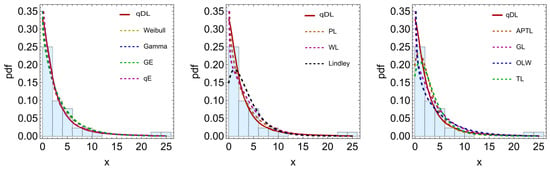
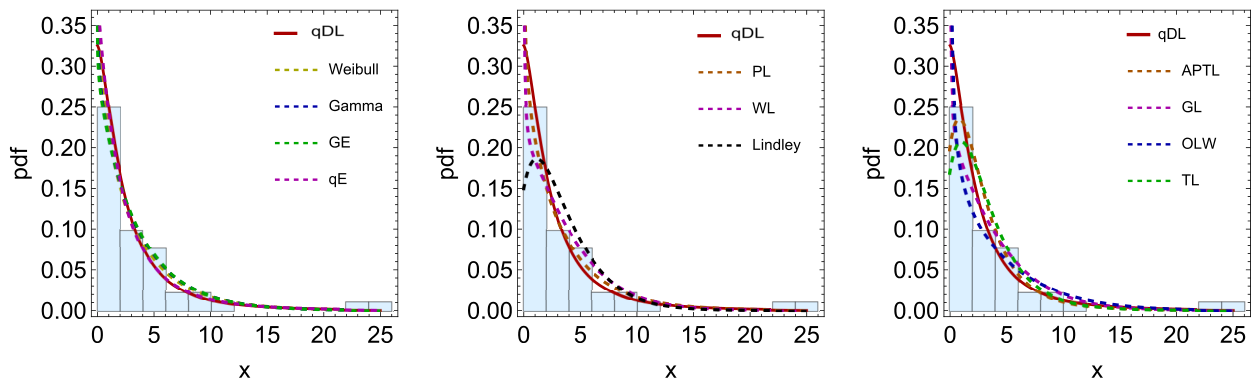
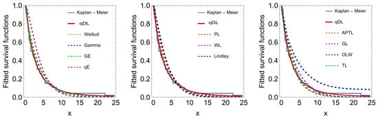
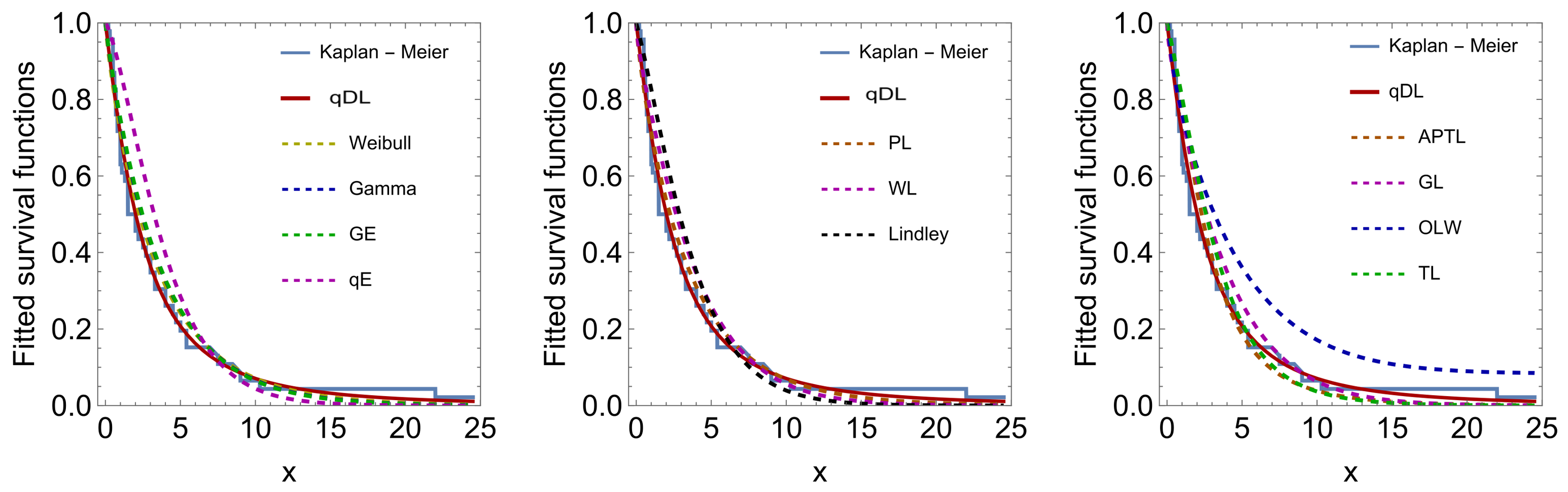
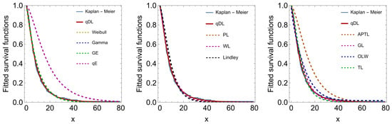
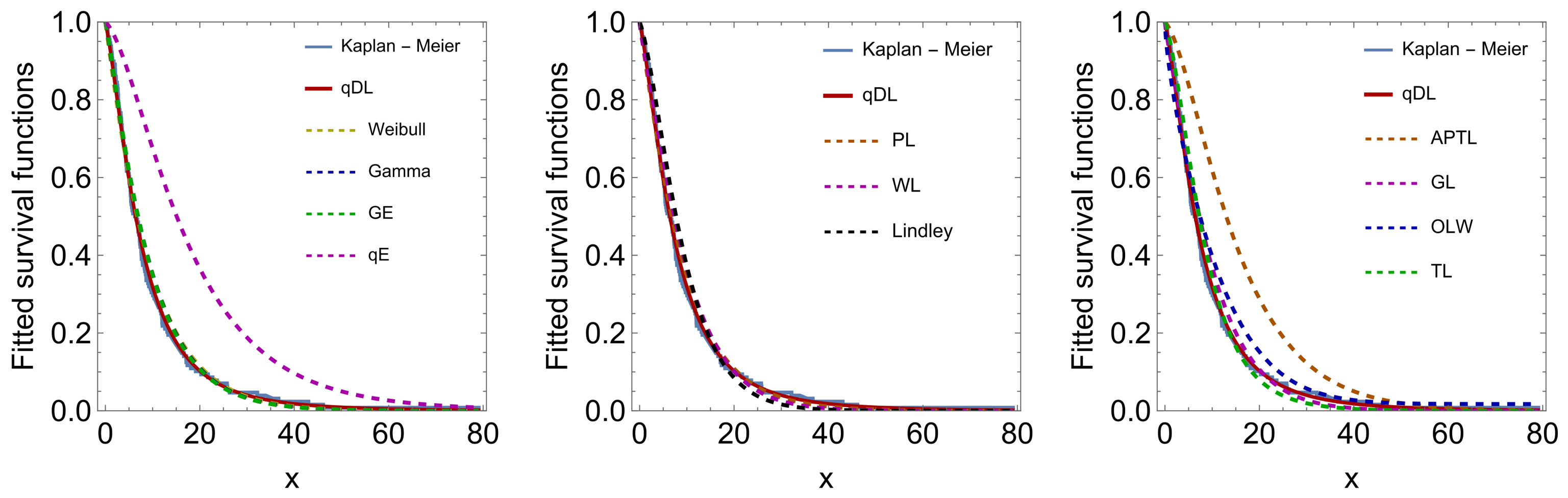
This section aims to illustrate the practical usefulness of the qDL distribution by comparing its performance with several well-known lifetime distributions, including the Weibull, Gamma, generalized exponential (GE), q-exponential (qE), Lindley, power Lindley (PL), weighted Lindley (WL), transmuted Lindley (TL), generalized Lindley (GL), alpha-power transformed Lindley (APTL), and two-parameter odd Lindley Weibull (OLW) distributions. The goodness-of-fit criteria used for the comparison are: Kolmogorov–Smirnov (KS) statistic along with its corresponding p-value, Akaike Information Criterion (AIC), Bayesian Information Criterion (BIC), Cramér–von Mises $\left(W^{*}\right)$, and Anderson–Darling $\left(A^{*}\right)$. In addition, graphical tools are employed to support the fitting results. In particular, the fitted probability density functions are overlaid on the histograms of the observed data, while the estimated survival functions are compared with the Kaplan–Meier estimator.

6.1. Repair Time Dataset

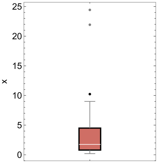
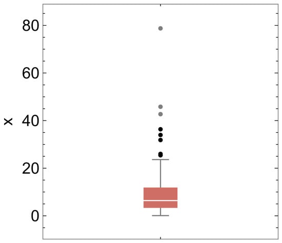
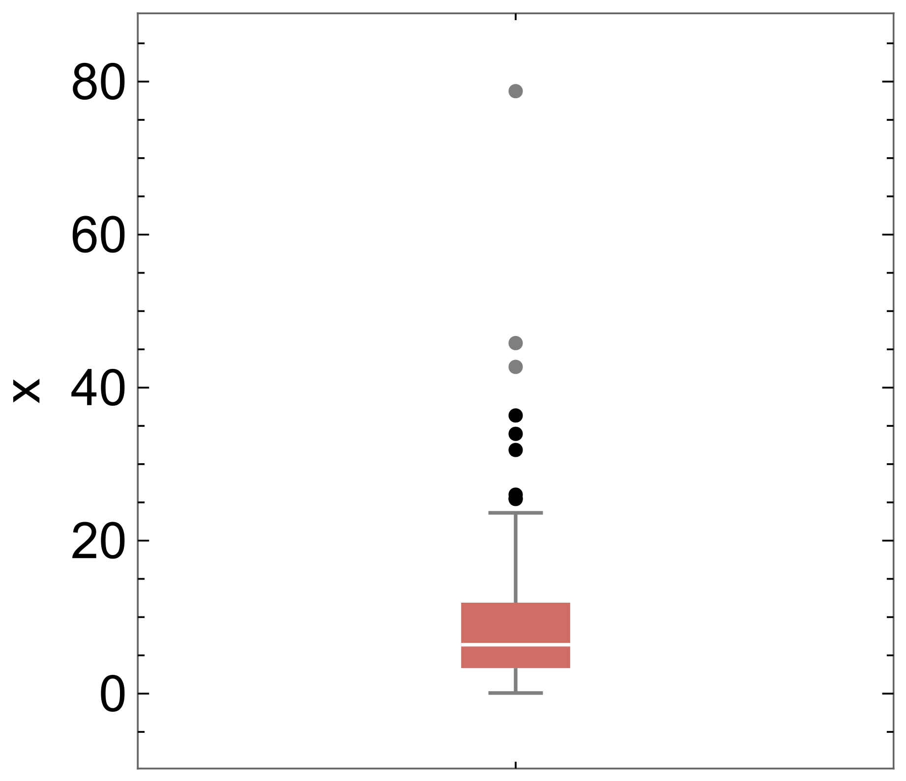
The dataset consists of active repair times (in hours) for an airborne communication transceiver, originally reported in [40]. The descriptive statistics in Table 6 indicate that the data are highly variable and right-skewed, with most observations being relatively small and a few extremely long repair times. The large positive skewness (2.89) and excess kurtosis (8.80) suggest a non-symmetric and heavy-tailed distribution. The box plot in Figure 4 further illustrates this pattern and highlights several extreme observations.

Table 6. Descriptive statistics of the repair time data.

n	Min	${\mathit{Q}}_1$	Median	Mean	${\mathit{Q}}_3$	Max	Range	IQR	Std. Dev.	Skewness	Kurtosis Excess
46	0.2	0.8	1.75	3.6065	4.5	24.5	24.3	3.7	4.9442	2.8883	8.8026

Figure 4. Box plot of the repair time data. Black dots indicate mild outliers, while gray dots indicate extreme outliers.

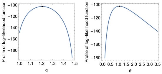
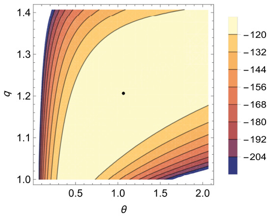
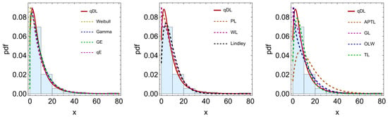
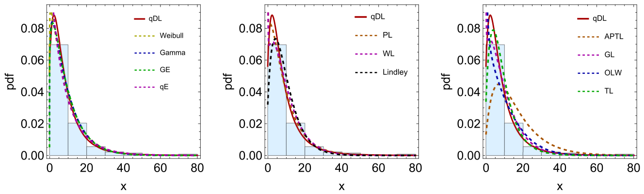
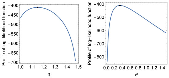
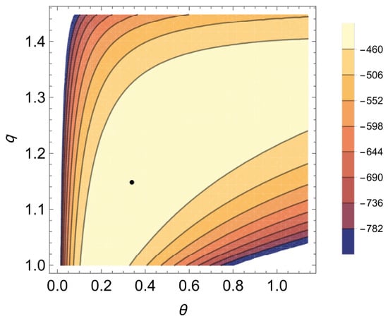
The estimated parameters and the goodness-of-fit measures for the fitted distributions are listed in Table 7. From this table, it is noted that the qDL distribution has the lowest KS, AIC, BIC, $\left(W^{*}\right)$, and $\left(A^{*}\right)$. Therefore, it provides the best fit for the data. Figure 5 and Figure 6 support this result by showing the estimated densities and estimated survival curves. To assess the uniqueness and stability of the MLEs of the qDL parameters, the profile log-likelihood functions of the parameters $\theta$ and q are examined and displayed in Figure 7, along with the corresponding contour plot of the log-likelihood surface in Figure 8. The plots show a single clear maximum, which suggests that the likelihood function is unimodal and that the MLEs are unique.

Table 7. MLEs and goodness-of-fit measures for the repair time data.

Model	MLEs		KS	p-Value	AIC	BIC	${\mathit{W}}^{*}$	${\mathit{A}}^{*}$
qDL	1.06546	1.20635	0.11283	0.60155	209.208	212.865	0.06579	0.54506
Weibull	0.89858	0.33375	0.12043	0.51699	212.939	216.597	0.12176	0.90324
Gamma	0.93229	3.86845	0.14542	0.28499	213.862	217.519	0.17716	1.12309
GE	0.26937	0.95828	0.151977	0.23848	213.966	217.623	0.19439	1.19389
q-exponential	0.49255	1.2198	0.12718	0.44645	209.909	213.566	0.07185	0.62973
PL	0.67573	0.75810	0.12600	0.45841	214.027	217.684	0.12475	0.94366
WL	0.36298	0.66292	0.17362	0.12488	220.253	223.911	0.28399	1.70593
TL	0.37420	0.64008	0.20241	0.04615	218.647	222.304	0.36579	2.19852
GL	0.36772	0.66430	0.16629	0.15704	219.698	223.355	0.27069	1.63903
APTL	0.26949	0.03707	0.16092	0.18452	213.451	217.109	0.19659	1.26159
OLW	0.48325	0.33315	0.18680	0.08070	224.117	227.774	0.62639	3.29596
Lindley	0.46637		0.23382	0.01308	221.969	223.798	0.57360	3.34023

Figure 5. Histogram of the repair time data with fitted densities.

Figure 6. Fitted survivals and Kaplan–Meier curve for repair time data.

Figure 7. Profile log-likelihood functions of $\theta$ and q for the repair time data.

Figure 8. Contour plot of the log-likelihood function for the repair time data. Colors indicate log-likelihood values.

6.2. Bladder Cancer Data

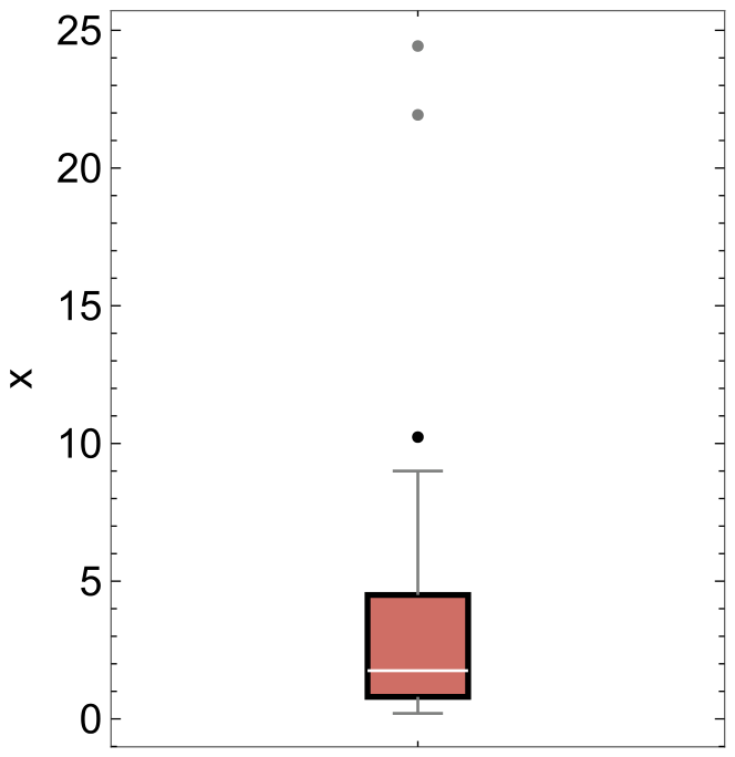
This dataset corresponds to remission times (in months) for patients diagnosed with bladder cancer. Data were reported in [41] and previously analyzed by [42]. The descriptive statistics in Table 8 indicate that bladder cancer remission times are highly variable and strongly right-skewed. The large positive skewness (3.29) and the extremely high excess kurtosis (15.48) suggest a marked right tail and heavy-tailed behavior. These features are further confirmed by the box plot in Figure 9, which clearly shows extreme observations.

Table 8. Descriptive statistics of the bladder cancer data.

n	Min	${\mathit{Q}}_1$	Median	Mean	${\mathit{Q}}_3$	Max	Range	IQR	Std. Dev.	Skewness	Kurtosis Excess
128	0.08	3.31	6.395	9.3656	11.79	79.05	78.97	8.55	10.5083	3.28657	15.4831

Figure 9. Box plot of the bladder cancer time data. Black dots indicate mild outliers, while gray dots indicate extreme outliers.

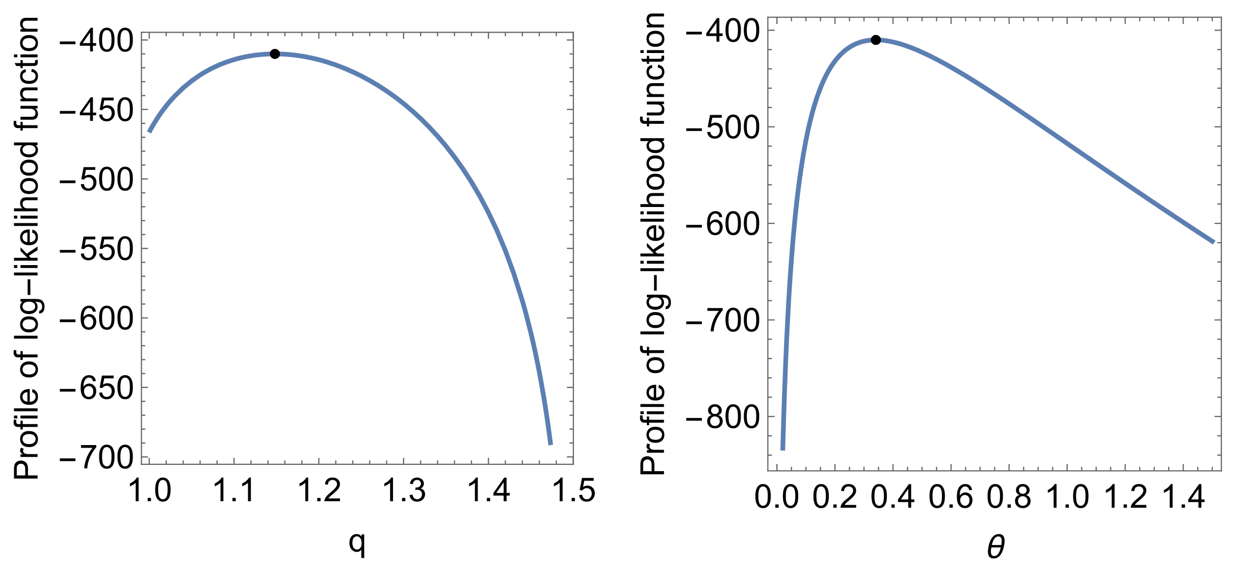
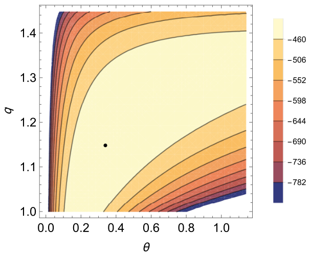
The parameter estimates and goodness-of-fit measures for the fitted models are reported in Table 9. The results indicate that the qDL distribution provides the best fit with the smallest values of the KS statistic and information criteria among the considered models. This conclusion is further supported by Figure 10 and Figure 11. The profile log-likelihood plots for the parameters $\theta$ and q, displayed in Figure 12, together with the contour plot in Figure 13, exhibit a single clear maximum, supporting the uniqueness of the MLEs.

Table 9. MLEs and goodness-of-fit measures for the bladder cancer data.

Model	MLEs		KS	p-Value	AIC	BIC	${\mathit{W}}^{*}$	${\mathit{A}}^{*}$
qDL	0.34087	1.14819	0.04793	0.93040	824.042	829.746	0.03845	0.24913
Weibull	1.04783	0.09389	0.07002	0.55697	832.174	837.878	0.15430	0.96345
Gamma	1.17251	7.98766	0.07329	0.49739	830.736	836.44	0.15430	0.96345
GE	0.12117	1.21795	0.07251	0.51132	830.155	835.859	0.12840	0.71819
q-exponential	0.12344	1.06694	0.09667	0.18270	831.666	837.37	0.21342	1.38504
PL	0.29433	0.83020	0.06823	0.59046	830.708	836.412	0.12734	0.79337
WL	0.15946	0.68276	0.09257	0.22273	836.884	842.589	0.25176	1.34896
TL	0.15577	0.61687	0.08985	0.25275	834.310	840.014	0.25189	1.44630
GL	0.16487	0.73363	0.09279	0.22039	836.572	842.276	0.24786	1.33202
APTL	0.11029	0.04179	0.05997	0.74660	826.769	832.473	0.08196	0.52847
OLW	0.27216	0.31511	0.11162	0.08237	854.058	859.762	0.52125	3.02679
Lindley	0.19605		0.11640	0.06233	841.06	843.912	0.52110	2.80200

Figure 10. Histogram of the bladder cancer data with fitted densities.

Figure 11. Fitted survival functions and Kaplan–Meier curve for the bladder cancer data.

Figure 12. Profile log-likelihood functions of $\theta$ and q for the bladder cancer data.

Figure 13. Contour plot of the log-likelihood function for the bladder cancer data. Colors indicate log-likelihood values.

7. Conclusions

This paper introduced the qDL distribution as a flexible generalization of the classical Lindley model under the Tsallis-q framework. The model accommodates both bounded and unbounded supports according to the value of the deformation parameter q, while retaining the Lindley distribution as a limiting case when $q\to 1$. This additional parameter substantially enhances the flexibility of the model by directly controlling the tail behavior and support structure, which makes the distribution suitable for modeling a wider range of right-skewed data than the classical Lindley model. From a theoretical perspective, several important structural properties of the qDL distribution were obtained in closed form, which confirms its analytical tractability and facilitates further statistical development. Multiple estimation procedures were investigated and compared through an extensive Monte Carlo simulation study. The results showed that the estimators perform satisfactorily across different parameter settings and sample sizes, with MLE and ADE generally providing superior performance. These findings provide useful guidance for practitioners regarding the choice of estimation technique in practical applications.

The practical value of the proposed model was further demonstrated through two applications to real right-skewed datasets. In both cases, the qDL distribution outperformed several well-known lifetime models, indicating that it can serve as a useful alternative in applied reliability, survival, and lifetime data analysis. Hence, the paper contributes both a new theoretically appealing distribution and a practically effective model for analyzing skewed data with diverse tail patterns.

There remain several directions for future research. One natural extension is to develop regression versions of the qDL distribution so that covariate effects can be incorporated in survival and reliability studies. It would also be worthwhile to investigate Bayesian inference, censored-data settings, record values, and stress–strength reliability measures for the proposed model. Such extensions would further enhance the usefulness of the proposed family and deepen its role in the analysis of nonstandard lifetime data.

References

- Lindley, D.V. Fiducial distributions and Bayes’ theorem. J. R. Stat. Soc. Ser. B 1958, 20, 102–107. [Google Scholar] [CrossRef] [Scilit]
- Ghitany, M.E.; Atieh, B.; Nadarajah, S. Lindley distribution and its application. Math. Comput. Simul. 2008, 78, 493–506. [Google Scholar] [CrossRef] [Scilit]
- Zakerzadeh, H.; Dolati, A. Generalized Lindley distribution. J. Math. Ext. 2009, 3, 13–25. [Google Scholar]
- Nadarajah, S.; Bakouch, H.S.; Tahmasbi, R. A generalized Lindley distribution. Sankhya B 2011, 73, 331–359. [Google Scholar] [CrossRef] [Scilit]
- Bakouch, H.S.; Al-Zahrani, B.M.; Al-Shomrani, A.A. An extended Lindley distribution. J. Korean Stat. Soc. 2012, 41, 75–85. [Google Scholar] [CrossRef] [Scilit]
- Ghitany, M.E.; Alqallaf, F.; Al-Mutairi, D.K.; Husain, H. A two-parameter weighted Lindley distribution and its applications to survival data. Math. Comput. Simul. 2011, 81, 1190–1201. [Google Scholar] [CrossRef] [Scilit]
- Ghitany, M.E.; Al-Mutairi, D.K.; Balakrishnan, N.; Al-Enezi, L. Power Lindley distribution and associated inference. Comput. Stat. Data Anal. 2013, 64, 20–33. [Google Scholar] [CrossRef] [Scilit]
- Shanker, R.; Mishra, A. A quasi Lindley distribution. Afr. J. Math. Comput. Sci. Res. 2013, 6, 64–71. [Google Scholar]
- Merovci, F. Transmuted lindley distribution. Int. J. Open Probl. Compt. Math. 2013, 6, 63–72. [Google Scholar] [CrossRef] [Scilit]
- Dey, S.; Ghosh, I.; Kumar, D. Alpha-power transformed Lindley distribution: Properties and associated inference with application to earthquake data. Ann. Data Sci. 2019, 6, 623–650. [Google Scholar] [CrossRef] [Scilit]
- Asgharzadeh, A.; Bakouch, H.S.; Nadarajah, S.; Sharafi, F. A new weighted Lindley distribution with application. Braz. J. Probab. Stat. 2016, 30, 1–27. [Google Scholar] [CrossRef] [Scilit]
- Abd El-Monsef, M. A new Lindley distribution with location parameter. Commun. Stat.-Theory Methods 2016, 45, 5204–5219. [Google Scholar] [CrossRef] [Scilit]
- Chesneau, C.; Tomy, L.; Gillariose, J. A new modified Lindley distribution with properties and applications. J. Stat. Manag. Syst. 2021, 24, 1383–1403. [Google Scholar] [CrossRef] [Scilit]
- Haj Ahmad, H.; Bdair, O.M.; Naser, M.F.M.; Asgharzadeh, A. The Rayleigh Lindley Distribution: A New Generalization of Rayleigh Distribution with Physical Applications. Rev. Investig. Oper. 2023, 44, 205–222. [Google Scholar]
- Bhati, D.; Malik, M.A.; Vaman, H. Lindley–exponential distribution: Properties and applications. Metron 2015, 73, 335–357. [Google Scholar] [CrossRef] [Scilit]
- Cakmakyapan, S.; Ozel, G. The Lindley family of distributions: Properties and applications. Hacet. J. Math. Stat. 2016, 46, 1113–1137. [Google Scholar] [CrossRef] [Scilit]
- Gomes-Silva, F.S.; Percontini, A.; de Brito, E.; Ramos, M.W.; Venâncio, R.; Cordeiro, G.M. The odd Lindley-G family of distributions. Austrian J. Stat. 2017, 46, 65–87. [Google Scholar] [CrossRef] [Scilit]
- Almamy, J.A.; Ibrahim, M.; Eliwa, M.; Al-mualim, S.; Yousof, H.M. The two-parameter odd Lindley Weibull lifetime model with properties and applications. Int. J. Stat. Probab. 2018, 7, 57. [Google Scholar] [CrossRef] [Scilit]
- Alizadeh, M.; Bagher, S.F.; Hou, J.c.; Nadarajah, S.; Shaban, A. The compound class of exponentiated power Lindley power series distribution: Properties and applications. Appl. Math.-J. Chin. Univ. 2025, 40, 255–275. [Google Scholar] [CrossRef] [Scilit]
- Saaidia, N.; Pakyari, R.; Zeghdoudi, H. The Q-Lindley Distribution: Goodness-of-Fit Tests, Modeling, Inference, and Applications. J. Stat. Theory Appl. 2026, 25, 6. [Google Scholar] [CrossRef] [Scilit]
- Imed, B.; Mouna, Z. The Lindley q-distribution: Properties and simulations. Ric. Mat. 2025, 74, 703–718. [Google Scholar] [CrossRef] [Scilit]
- Tsallis, C. Possible generalization of Boltzmann–Gibbs statistics. J. Stat. Phys. 1988, 52, 479–487. [Google Scholar] [CrossRef] [Scilit]
- Mathai, A. A pathway to matrix-variate gamma and normal densities. Linear Algebra Its Appl. 2005, 396, 317–328. [Google Scholar] [CrossRef] [Scilit]
- Tsallis, C. Nonextensive Statistical Mechanics and Thermodynamics: Historical Background and Present Status. In Nonextensive Statistical Mechanics and Its Applications; Lecture Notes in Physics; Abe, S., Okamoto, Y., Eds.; Springer: Berlin/Heidelberg, Germany, 2001; Volume 560, pp. 3–98. [Google Scholar] [CrossRef] [Scilit]
- Picoli, S., Jr.; Mendes, R.; Malacarne, L. q-exponential, Weibull, and q-Weibull distributions: An empirical analysis. Phys. A Stat. Mech. Its Appl. 2003, 324, 678–688. [Google Scholar] [CrossRef] [Scilit]
- Jose, K.; Naik, S.R. On the q-Weibull distribution and its applications. Commun. Stat. Methods 2009, 38, 912–926. [Google Scholar] [CrossRef] [Scilit]
- Mathai, A.; Provost, S.B. On q-logistic and related models. IEEE Trans. Reliab. 2006, 55, 237–244. [Google Scholar] [CrossRef]
- Picoli, S., Jr.; Mendes, R.S.; Malacarne, L.C.; Santos, R.P.B. q-distributions in complex systems: A brief review. Braz. J. Phys. 2009, 39, 468–474. [Google Scholar] [CrossRef] [Scilit]
- Mathai, A.; Provost, S.B. The q-extended inverse Gaussian distribution. J. Probab. Stat. Sci. 2011, 9, 1–20. [Google Scholar]
- Kumar, N.; Dixit, A.; Vijay, V. q-Generalization of Nakagami distribution with applications. Jpn. J. Stat. Data Sci. 2025, 8, 69–92. [Google Scholar] [CrossRef] [Scilit]
- de la Barra, E.; Vega-Jorquera, P. On q-pareto distribution: Some properties and application to earthquakes. Eur. Phys. J. B 2021, 94, 32. [Google Scholar] [CrossRef] [Scilit]
- Provost, S.B.; Saboor, A.; Cordeiro, G.M.; Mansoor, M. On the q-generalized extreme value distribution. REVSTAT-Stat. J. 2018, 16, 45–70. [Google Scholar]
- Eliwa, M.S.; Zaid, E.A.; El-Morshedy, M. ON q-generalized extreme values under power normalization with properties, estimation methods and applications to COVID-19 data. REVSTAT-Stat. J. 2024, 22, 61–86. [Google Scholar]
- Preda, V.; Catana, L.I. Tsallis Log-Scale-Location Models. Moments, Gini Index and Some Stochastic Orders. Mathematics 2021, 9, 1216. [Google Scholar] [CrossRef] [Scilit]
- Zhang, F.; Shi, Y.; Keung Tony Ng, H.; Wang, R. Tsallis statistics in reliability analysis: Theory and methods. Eur. Phys. J. Plus 2016, 131, 379. [Google Scholar] [CrossRef] [Scilit]
- Da Silva, G.; Ramos, R. The lambert–tsallis wq function. Phys. A Stat. Mech. Its Appl. 2019, 525, 164–170. [Google Scholar] [CrossRef] [Scilit]
- Yamano, T. Some properties of q-logarithm and q-exponential functions in Tsallis statistics. Phys. A Stat. Mech. Its Appl. 2002, 305, 486–496. [Google Scholar] [CrossRef] [Scilit]
- Cordeiro, G.; Silva, R.; Nascimento, A. Recent Advances in Lifetime and Reliability Models; Bentham Science Publishers: Singapore, 2020. [Google Scholar]
- Cheng, R.C.H.; Amin, N.A.K. Maximum product of spacings estimation with application to the Weibull distribution. J. R. Stat. Soc. Ser. B (Methodol.) 1979, 41, 354–367. [Google Scholar]
- Jorgensen, B. Statistical Properties of the Generalized Inverse Gaussian Distribution; Springer Science & Business Media: Berlin/Heidelberg, Germany, 2012; Volume 9. [Google Scholar]
- Lee, E.T.; Wang, J. Statistical Methods for Survival Data Analysis; John Wiley & Sons: Hoboken, NJ, USA, 2003; Volume 476. [Google Scholar]
- Rady, E.H.A.; Hassanein, W.; Elhaddad, T. The power Lomax distribution with an application to bladder cancer data. SpringerPlus 2016, 5, 1838. [Google Scholar] [CrossRef] [Scilit]
Disclaimer/Publisher’s Note: The statements, opinions and data contained in all publications are solely those of the individual author(s) and contributor(s) and not of MDPI and/or the editor(s). MDPI and/or the editor(s) disclaim responsibility for any injury to people or property resulting from any ideas, methods, instructions or products referred to in the content. |
© 2026 by the authors. Licensee MDPI, Basel, Switzerland. This article is an open access article distributed under the terms and conditions of the Creative Commons Attribution (CC BY) license.