


Abstract
To improve the decoding performance of multi-edge type low-density parity-check (MET-LDPC) codes, this paper proposes an edge-type differentiated parameter coupling offset min-sum (EDPC-OMS) decoding algorithm. The contributions are threefold. First, we replace the traditional uniform compensation with edge-type differentiated compensation, resolving the mismatch between the decoding model and code structure. Second, we introduce a parameter coupling mechanism that enables joint optimization of multiple edge types while maintaining differentiated configurations. Third, a practically feasible design combining precomputation and look-up tables enables dynamic parameter adjustment with moderate additional overhead, achieving a favorable performance–complexity trade-off. Simulation results over additive white Gaussian noise (AWGN) channels and Rayleigh fading channels demonstrate that the proposed algorithm adaptively selects offset factors according to channel conditions and edge types without introducing significant computational complexity, effectively lowering the bit error rate and enhancing decoding capability.
Keywords:
MET-LDPC codes; EDPC-OMS; edge-type differentiated compensation; parameter coupling mechanism; dynamic parameter adjustment MSC:
94.B35
1. Introduction
Low-Density Parity-Check (LDPC) codes [1,2,3], first introduced by Gallager in 1962, are a family of linear block codes characterized by a sparse parity-check matrix. Owing to their near-Shannon-limit error-correcting performance, highly parallelizable decoding structure, and relatively low implementation complexity, LDPC codes have attracted extensive research interest over the past few decades.
LDPC decoding algorithms generally fall into two types, namely hard-decision [4] and soft-decision decoding [5]. Hard-decision decoding is simple to implement. However, it does not make full use of the probabilistic information from the channel, so its error-correction capability is limited. Soft-decision decoding, on the other hand, exploits richer channel information and thus achieves much better performance. The Belief Propagation (BP) algorithm [6], is a classic example of soft-decision decoding. It works by iteratively passing messages between variable and check nodes, approaching the Shannon limit. Despite its theoretical strength, the BP algorithm involves heavy computations. Specifically, the check node updates require multiplications of hyperbolic tangent functions and their inverses. This complexity makes hardware implementation difficult, especially when resources are limited.
To reduce the computational complexity of the BP algorithm, the Min-Sum (MS) decoding algorithm was proposed [7]. This approach takes advantage of the mathematical properties of the hyperbolic tangent function. It turns the complex multiplications in check node updates into simple comparisons and additions. As a result, implementation becomes much easier. However, this simplification comes at a cost. It systematically overestimates the output information from the check nodes. Therefore, compared to the BP algorithm, its performance drops noticeably. Later, researchers proposed two improved algorithms to strike a better balance between complexity and performance. These are the normalized min-sum (NMS) [8,9] and the offset min-sum (OMS) algorithms [10,11,12]. Both follow a simple linear post-processing idea. The NMS algorithm scales down the overestimated MS outputs by multiplying them by a factor less than one. The OMS algorithm, on the other hand, subtracts a positive offset to correct the estimation bias. These two methods effectively bring the MS algorithm closer to BP in terms of performance. They achieve this with very little extra computational cost. That is why they have become two of the most widely used LDPC decoding schemes in practical engineering.
While conventional LDPC decoding schemes have become increasingly mature, the introduction of Multi-Edge Type Low-Density Parity-Check (MET-LDPC) codes [13,14,15] has opened a new path for further performance improvement. However, this advancement also imposes higher demands on the refined design of decoding algorithms. As an important extension of conventional LDPC codes, MET-LDPC codes construct a more flexible factor graph structure by introducing multiple types of variable nodes, check nodes, and the diverse edge types connecting them. This enhanced structural flexibility endows MET-LDPC codes with theoretical performance beyond that of traditional LDPC codes, particularly exhibiting significant advantages in the short-to-moderate block length and high-rate regimes. However, the structural complexity of MET-LDPC codes also implies notable disparities among different edge types in terms of channel conditions, node degrees, and information evolution during the iterative process. This, in turn, requires decoding algorithms to possess a correspondingly refined processing capability.
Recent research on decoding algorithms for MET-LDPC codes has primarily progressed along two complementary directions, namely optimizing the decoding schedule and adjusting normalization factors. These two approaches explore performance enhancement from the perspectives of structural organization and parameter configuration, respectively.
In terms of scheduling optimization, efforts have focused on adapting the timing and topology of message passing to accommodate the multi-edge characteristics of MET-LDPC codes. To resolve memory access conflicts in layered belief propagation decoding of multi-edge type quasi-cyclic LDPC codes, a cross-layer scheduling (CLS) method was proposed in [16]. This technique pairs and alternately updates layers with small common degrees, reducing memory conflicts without compromising decoding performance. From a structural perspective, Reference [17] partitions the Tanner graph into three regions based on edge types and introduces region-specific message scaling factors to adaptively control information exchange between regions. The resulting regional message scaling min-sum (RMS) decoding framework achieves preliminary adaptation to the multi-edge structure of MET-LDPC codes at the scheduling level.
In the direction of normalization factor adjustment, references [18,19,20] extend the study of normalization factor optimization to MET-LDPC codes with two edge types, aiming to improve the performance of the NMS algorithm. Reference [18] proposes a neural NMS algorithm based on deep learning to learn optimal parameters. Reference [19] enhances multi-edge density evolution to predict asymptotic performance and introduces an adaptive quantized NMS algorithm that balances precision and complexity. Reference [20] theoretically analyzes the performance loss of the MS algorithm relative to the sum-product algorithm across edge types and uses density evolution to efficiently search for optimal normalization factors, offering a theoretical basis for parameter configuration.
A review of the aforementioned studies reveals a common limitation. Specifically, neither the optimization of the OMS algorithm for conventional LDPC codes, nor the scheduling strategies and normalization factor adjustments tailored for MET-LDPC codes, have considered the inherent relationship between the multiple edge types of MET-LDPC codes and the offset factor. This limitation is particularly evident in existing studies on MET-LDPC codes. On one hand, scheduling optimization works (e.g., [16,17]) focus on the timing and structural organization of message passing, but fail to address the fine-grained correction of message amplitudes. On the other hand, while normalization factor adjustment works (e.g., [18,19,20]) optimize parameters, they are confined to a single, global normalization factor and have not yet incorporated the offset factor, a core parameter of the OMS algorithm, into their research scope.
A direct consequence of this research gap is that existing OMS decoding algorithms, when applied to MET-LDPC codes, continue to adopt the single-edge-type processing paradigm originally designed for conventional LDPC codes. By treating MET-LDPC codes as ordinary irregular LDPC codes, these approaches completely overlook the heterogeneous characteristics of different edge types during message propagation. This mismatch between the code structure and the decoding algorithm prevents MET-LDPC codes from realizing their full performance potential. Essentially, applying a single-edge-type algorithm to multi-edge-type codes constitutes a structural misalignment between the decoding model and the code structure.
Motivated by this observation, this paper proposes an edge-type differentiated parameter coupling offset min-sum (EDPC-OMS) decoding algorithm for MET-LDPC codes. The main contributions of this paper are as follows.
- First, for MET-LDPC codes, we establish a mapping between edge types and correction parameters. Unlike conventional approaches that apply uniform correction across all edge types, the proposed method assigns asymmetric offset factors to check nodes according to different edge types. This enables fine-grained, differentiated message correction aligned with the code structure, fundamentally resolving the structural mismatch between the decoding model and the code.
- Second, we propose the EDPC-OMS decoding algorithm for MET-LDPC codes. Central to this algorithm is a parameter coupling mechanism specifically designed for the collaborative optimization of multiple edge types. By recognizing the interdependence of correction processes across different edge types, this mechanism leverages information correlations during iterative decoding to jointly optimize and dynamically adjust the offset factors.
- Third, we design a practically efficient implementation scheme using precomputation and look-up tables. Although the proposed algorithm introduces moderately more arithmetic operations than CLS or RMS, it achieves consistently better BER performance, offering a well-balanced performance–complexity trade-off.
The remainder of this paper is organized as follows. Section 2 introduces MET-LDPC codes and decoding algorithms. Section 3 presents the impact of unified offset configuration on decoding performance. Section 4 elaborates on the proposed EDPC-OMS decoding algorithm. Section 5 provides simulation results and performance analysis. Finally, Section 6 concludes the paper.
2. MET-LDPC Codes and Decoding Algorithms
Multi-Edge Type Low-Density Parity-Check (MET-LDPC) codes generalize conventional LDPC codes by incorporating multiple node and edge types, enabling a richer description of code structures. This flexibility allows them to approach channel capacity in a wider range of communication scenarios, including asymmetric channels [21], high-order modulation [22], and rate-compatible systems [23]. The resulting structural complexity, however, calls for decoding algorithms that account for edge-type heterogeneity to ensure efficient message passing. This section provides an overview of MET-LDPC code fundamentals and a systematic review of their classical decoding algorithms, culminating in the MS algorithm and its variants. These foundations pave the way for the EDPC-OMS decoding algorithm introduced in subsequent section.
2.1. Fundamentals of MET-LDPC Codes
MET-LDPC codes represent a structural generalization of conventional LDPC codes. In the Tanner graph of conventional LDPC codes, all variable nodes and check nodes can be regarded as homogeneous, and their connecting edges are not distinguished by type. In contrast, MET-LDPC codes classify nodes and edges into multiple types, employing multi-dimensional distribution parameters to characterize the connections between different node types and edge types. This enables a more refined description and control of the code structure.
Formally, the Tanner graph of an MET-LDPC code can be defined as a quadruple , with the following components.
- Variable node set . The set of nodes representing codeword bits. can be further partitioned into multiple disjoint subsets aswhere is the total number of variable node types, and denotes the set of variable nodes of the k-th type. Different types of variable nodes may correspond to distinct channel transmission characteristics, degree distribution requirements, or protection priorities.
- Check node set . The set of nodes representing parity-check constraints. can be further partitioned into multiple disjoint subsets aswhere Z is the total number of check node types, and denotes the set of check nodes of the z-th type. Different types of check nodes may correspond to different constraint equations or check strengths.
- Edge type set . The set of all possible edge typeswhere is the total number of edge types. The type of an edge is closely related to, but not uniquely determined by, the types of the two nodes it connects. Multiple distinct edge types may exist between the same pair of node types, endowing MET-LDPC codes with enhanced structural descriptive capability.
- Edge set . The set of connections between variable nodes and check nodes. According to edge types, the edge set can be further partitioned into multiple disjoint subsets aswhere denotes the set of edges of the t-th type, with . Each edge connects the n-th variable node and the m-th check node, and belongs to exactly one edge type subset , i.e., .
Figure 1 shows the graphical representation [24] of an MET-LDPC code with the rate 0.5. It can be represented as , where , , , and .
Figure 1.
Graphical representation of the MET-LDPC code. Variable nodes and check nodes are depicted as solid circles (●) and squares (□), respectively. The numbers labeled on the edges indicate the quantity of each edge type incident to the corresponding node. N is the number of transmitted code bits.
Based on the edge-type connection structure, the factor graph of MET-LDPC codes can be partitioned into three functional regions [17], namely the low-reliability information injection region (LIR) composed of degree-1 edges and their connected nodes, the high-reliability information aggregation region (HAR) composed of degree-2 accumulated edges and their connected nodes, and the adaptive information relay region (ARR) centered on punctured variable nodes. These three regions involve two types of check nodes, denoted as and , which correspond to the HAR and LIR, respectively.
This refined structural design enables MET-LDPC codes to adapt more flexibly to channel characteristics. By adjusting the distribution of different edge types, the propagation paths and convergence behavior of messages in the Tanner graph can be controlled, thereby achieving theoretical performance closer to channel capacity than conventional LDPC codes. However, this structural advantage also imposes higher demands on the design of decoding algorithms. The decoding process must fully account for the heterogeneity of edge types and adopt differentiated message processing strategies for different edge types to optimize message-passing efficiency.
2.2. BP Decoding Algorithm
The BP algorithm is the standard iterative decoding method for LDPC-like codes. Traditional probability-domain BP algorithms involve a large number of multiplication operations, resulting in high computational complexity and poor numerical stability. The log-likelihood ratio belief propagation (LLR-BP) algorithm was proposed to address these issues, which converts multiplication operations in the probability domain into addition operations in the logarithmic domain by introducing log-likelihood ratios (LLR). This conversion significantly reduces complexity and enhances stability, establishing LLR-BP as the mainstream decoding scheme in practical applications.
For MET-LDPC codes, the LLR-BP decoding process aligns conceptually with that of traditional LDPC codes. However, message passing must be modeled with explicit consideration of edge type differentiation. To facilitate the description of the proposed LLR-BP decoding algorithm for MET-LDPC codes, the key notations are defined in Table 1.
Table 1.
Notation for the LLR-BP decoding algorithm of MET-LDPC codes.
The core of LLR-BP decoding lies in the check node update strictly following the tanh rule. Moreover, messages of different edge types are processed independently during updates. The specific decoding steps are as follows.
- (1)
- Initialization
Consider a binary encoded sequence modulated by binary phase shift keying (BPSK) and transmitted over an additive white Gaussian noise (AWGN) channel. The received sequence at the decoder is denoted as . The initial LLR for variable node , derived from the channel output, is given by
where represents the transmitted bit and is the channel noise variance.
- (2)
- Check Node Update
For message update along an edge of type t, each check node aggregates incoming messages from all neighboring variable nodes, processes them, and transmits updated messages to each neighboring variable node , excluding the source node. The update rule, which incorporates the type characteristics of connecting edges, is expressed as
- (3)
- Variable Node Update
Upon receiving messages from neighboring check nodes, each variable node updates its posterior LLR by combining these messages with its intrinsic channel information, subsequently transmitting new messages to each neighboring check node. The message update along an edge of type t is calculated as
- (4)
- Decoding Decision
The posterior LLR for each variable node is computed by aggregating messages across all incident edge types
For each variable node , hard decision decoding is performed based on the posterior LLR. The hard decision bit is determined by
yielding the decoded codeword The iterative process terminates when either the parity check condition is satisfied or the predetermined maximum number of iterations is reached, at which point the decoding result is output. Otherwise, the algorithm proceeds to the next iteration by returning to step (2).
2.3. OMS Decoding Algorithm
Despite the computational advantages conferred by logarithmic domain transformation, the LLR-BP algorithm still necessitates tanh and tanh−1 operations in its check node update formulation, which typically require complex table lookup procedures in hardware implementations, thereby consuming substantial logic resources. To circumvent this bottleneck, the MS decoding algorithm was developed.
The fundamental innovation of the MS algorithm lies in approximating the computationally intensive tanh product operation in the LLR-BP algorithm with a simplified min-sum operation. For MET-LDPC codes, the check node update in Equation (6) can be expressed as
where the sign is defined as
and the magnitude can be obtained by
This approximation effectively transforms complex multiplication operations into elementary comparison and addition operations, dramatically reducing computational complexity and hardware implementation difficulty. However, the magnitude of check node messages estimated by the MS algorithm consistently exceeds or equals the true values computed by the LLR-BP algorithm. This overestimation phenomenon inevitably incurs significant decoding performance degradation.
To mitigate the performance loss of the MS algorithm while preserving its low-complexity advantage, several enhanced variants have been proposed, among which the NMS and offset OMS algorithms are most prominent. Both approaches modify the amplitude of messages output by the MS algorithm to more accurately approximate LLR-BP performance.
- NMS Algorithm: Introduces a normalization factor to scale the overall amplitude of MS-output messages, thereby compensating for overestimation. By introducing a multiplicative correction factor α, the check node message update calculation is modified by
- OMS Algorithm: Introduces an offset factor to subtract a positive value from the minimum amplitude computed by the MS algorithm, effectively reducing overestimation. For MET-LDPC codes, the magnitude in the check node update formula for the OMS algorithm must explicitly incorporate edge type differentiation, which is expressed as
The NMS and OMS algorithms, by achieving a favorable balance between decoding performance and computational complexity, have become the most widely used LDPC decoding schemes. However, for the more structurally complex MET-LDPC codes, where multiple types of edges exist in the Tanner graph, messages conveyed on different types of edges often exhibit significantly different statistical characteristics. The traditional OMS algorithm employs a single, globally fixed offset factor , which struggles to accurately match the message distribution characteristics of all edge types, leaving room for further improvement in decoding performance. Therefore, exploring decoding algorithms with differentiated parameter optimization for different edge types holds significant theoretical importance and practical value for fully exploiting the structural potential of MET-LDPC codes and achieving decoding performance approaching the capacity limit.
2.4. Edge-Type-Based Layered Scheduling
Layered scheduling [25,26] is a message-passing strategy aimed at enhancing both the decoding performance and efficiency of MET-LDPC codes through structured hierarchical processing. MET-LDPC codes extend the conventional LDPC framework by incorporating multiple edge types, thereby overcoming the limitations of codes that rely on a single statistical edge type and enabling the construction of more flexible and expressive Tanner graphs. In this framework, variable nodes are classified into distinct node types according to the specific combination of incident edge types, where each node type is associated with a particular degree distribution and channel connection profile.
Unlike conventional flooding scheduling [27], in which all messages are updated simultaneously, the decoding process for MET-LDPC codes employs an edge-type-based layered scheduling strategy. As shown in Figure 1, the parity-check matrix is partitioned into multiple layers. Each layer corresponds to a specific set of edge types and is located in a particular region. Message updates are performed sequentially on a layer-by-layer basis, following the order of edge types. In contrast to traditional layered scheduling, which partitions the matrix by rows or columns, the proposed edge-class-based approach emphasizes the topological structure of message passing. Within each layer, all nodes share the same edge-type characteristics. The propagation of messages between these layers is governed by the inherent dependencies among the edge types. This mechanism achieves more efficient information exchange and faster convergence.
In this work, to mitigate the limitation of slow convergence inherent in conventional decoding algorithms, we adopt a layered scheduling strategy to enhance the decoding speed.
3. Impact of Unified Offset Configuration on Decoding Performance
The uniform offset represents the most fundamental parameter configuration in the OMS decoding algorithm. This approach treats all check nodes as homogeneous by assigning the same offset factor to every check node. The performance characteristics of the uniform-offset min-sum (UOMS) decoding algorithm under various channel conditions serve as a benchmark for subsequent optimization efforts. Therefore, before investigating the edge-type differentiated parameter coupling optimization method, it is necessary to systematically characterize the decoding behavior under the conventional uniform offset configuration, thereby clarifying the applicable scope and inherent limitations of the existing approach.
This section quantitatively investigates the impact of the uniform offset factor on the bit error rate performance of MET-LDPC codes through Monte Carlo simulations. The analysis focuses on the following two aspects, namely the influence intensity of the offset parameter in different signal-to-noise ratio (SNR) regions and the evolution trajectory of the optimal offset factor. This analysis aims to reveal the intrinsic relationship between the offset parameter and channel conditions, thereby establishing an experimental foundation and theoretical basis for the subsequent investigation of partition-based optimization strategies.
3.1. Simulation Parameter Configuration
To systematically evaluate the impact of the unified offset, the simulation parameters are set as shown in Table 2.
Table 2.
Simulation parameters for UOMS decoding algorithm.
3.2. Impact of Unified Offset on BER at Different SNR Levels
To comprehensively evaluate the impact of unified offset on system performance under different channel conditions, this section systematically investigates the effect of the unified offset parameter on the BER as the SNR varies.
Figure 2 presents the BER as a function of the offset parameter under various SNR conditions, illustrating the coupling relationship between the two. From Figure 2a, it can be observed that the effect of the offset on system BER performance is highly dependent on the SNR level, exhibiting distinct characteristics across different SNR regions. According to the experimental results, there exists a globally optimal fixed offset value of 0.2 for the system. Across a wide SNR range from 0.6 dB to 2.0 dB, this offset value consistently maintains optimal or near-optimal BER performance. In the low SNR region (≤0.8 dB), the offset has a limited impact on performance, with offsets of 0.2 and 0.3 showing relatively better results. In the medium-to-high SNR region (>0.8 dB), the advantage of becomes significant, and the performance gap widens as SNR increases.
Figure 2.
BER versus offset curves at different SNR (dB) levels. (a) Overview of BER versus offset factor under various SNR conditions. (b) BER versus offset factor at representative SNRs with 95% confidence interval error bars.
Figure 2b presents the BER versus offset factor β curves at SNR = 0.8 dB and 1.4 dB with 95% confidence interval error bars. These error bars are calculated based on 100 bit errors per point, yielding a relative half-width of ±19.6%. The following observations can be made. At SNR = 0.8 dB, the optimal offset range is β = 0.1 to 0.3, and the error bar analysis confirms that the BER differences between this optimal range and the degraded region where β ≥ 0.5 are statistically significant. At SNR = 1.4 dB, the optimal offset precisely converges to β = 0.2, and a pronounced cliff effect occurs when β ≥ 0.5, where the BER increases by approximately 160 times as β increases from 0.2 to 0.6. Notably, the error bars for the two curves do not overlap between the optimal region and the cliff region, confirming that the observed performance differences are not attributable to simulation noise. This verifies the significant impact of the offset parameter on the decoding performance of MET-LDPC codes and its high sensitivity characteristic.
3.3. Three-Dimensional Performance Surface Analysis
Building upon the two-dimensional analysis presented in Section 3.2, this section constructs a three-dimensional performance surface that integrates both SNR and offset variations into a unified visualization.
Figure 3 illustrates the impact of different decoding offset values and SNR on the BER in the UOMS decoding algorithm. The X-axis represents the normalized decoding offset , ranging from 0.0 to 1.0. The Y-axis represents the SNR, ranging from 0.0 to 2.0. The Z-axis represents the base-10 logarithm of the bit error rate (log10(BER)), providing an intuitive visualization of the order-of-magnitude variations in BER under different parameter combinations.
Figure 3.
Three-dimensional representation of BER performance against SNR and offset .
The surface employs a colormap to represent the Z-axis values, with colors ranging from dark to light corresponding to high and low log10(BER) values, respectively. In this figure, dark purple regions indicate a higher bit error rate, while light yellow regions correspond to a lower bit error rate. The continuous and smooth transition of the surface intuitively illustrates the overall trend of the bit error rate as it varies with changes in the SNR and decoding offset. The red scatter points superimposed on the figure represent the actual measured data points. Their close alignment with the surface validates the accuracy of the surface fitting to the experimental data.
The three-dimensional performance surface analysis reveals that the UOMS algorithm exhibits significant canyon structure, asymmetry, and cliff effect. As SNR increases, the performance valley gradually deepens and narrows around the optimal offset of 0.2, indicating that the system becomes highly sensitive to offset deviations under high SNR conditions. The surface displays pronounced asymmetry, with negative deviations causing gradual performance degradation while positive deviations lead to severe deterioration, suggesting that selecting a slightly smaller offset is a more prudent strategy when precise control is not feasible. When SNR exceeds 1.6 dB, the surface drops sharply forming a performance cliff, where the offset becomes the dominant limiting factor. At 2.0 dB, the valley bottom is extremely narrow, highlighting the critical importance of precise offset control in high SNR regimes.
Three-dimensional surface analysis further confirms the existence of a globally optimal fixed offset of 0.2. However, the valley structure, asymmetry, and cliff effect revealed by the surface also highlight the inherent limitations of the unified offset approach from another perspective.
The UOMS algorithm adopts a uniform offset correction approach, treating all edge types of MET-LDPC codes as homogeneous entities under the assumption that they exhibit similar overestimation characteristics and can share the same compensation parameter. However, the fundamental advantage of MET-LDPC codes lies precisely in enhancing coding flexibility and performance potential through multiple edge types. Different edge types inherently differ in degree distribution, connection structure, and message propagation paths, theoretically requiring distinct offset responses. Although the uniform correction method identifies a global compromise solution, it lacks the capability for differentiated adjustments. The canyon structure in Figure 3 suggests that assigning independent offsets to different edge types could carve deeper and wider performance valleys, unlocking the latent gains of MET-LDPC codes. This finding transcends the limitations of the uniform correction approach and establishes a theoretical foundation for subsequent optimization methods based on edge-type differentiation.
4. The Proposed EDPC-OMS Decoding Algorithm
To address the limitations of the UOMS algorithm revealed in Section 3, this section proposes a promising improved scheme, namely the EDPC-OMS decoding algorithm. The core of this algorithm is a parameter coupling mechanism specifically designed for the collaborative optimization of multiple edge types. This mechanism leverages the information correlation in iterative decoding to jointly optimize and dynamically adjust the offset factors for different edge types.
In terms of specific implementation, the algorithm performs layered classification of the check nodes of MET-LDPC codes based on edge types. Specifically, all edges are grouped into several mutually disjoint sets according to their types, with each set corresponding to a layer of check nodes that share the same connection characteristics for that edge type. Check nodes within the same layer share a common offset parameter, while different layers can employ distinct offset values. Since different edge types exhibit distinct statistical characteristics and overestimation tendencies, this differentiated offset configuration enables more precise correction of the reliability of messages for each edge type. Furthermore, the parameter coupling mechanism exploits the synergistic gains among multiple edge types, thereby achieving decoding performance superior to that of the uniform offset approach.
4.1. Edge-Type Differentiated Offset Configuration
In the check node structure of MET-LDPC codes, based on the differences in edge types, the check nodes can be partitioned into two functionally distinct layers, namely the HAR layer and the LIR layer. This section proposes an edge-type differentiated offset configuration scheme, which assigns independent offset factors to different edge-type layers according to their reliability characteristics, thereby enabling more precise message correction during check node updates.
4.1.1. Definition of the HAR and LIR Layers
The HAR layer consists of check nodes connected to high-reliability edge types, which typically correspond to bits requiring stronger protection or carrying critical information. These check nodes enforce stringent parity constraints to ensure reliable transmission. Messages exchanged between variable nodes and HAR layer check nodes exhibit higher confidence during decoding.
The LIR layer, conversely, comprises check nodes connected to low-reliability edge types. These edges correspond to bits with weaker protection requirements or higher error tolerance. The LIR layer provides flexible parity constraints, enabling higher code rates or better adaptability to specific channel conditions. Messages in this layer carry lower confidence and may employ different processing strategies.
This hierarchical structure embodies the design philosophy of MET-LDPC codes, where edge-type differentiation enables optimized decoding through layer-specific processing.
4.1.2. Edge-Type-Aware Offset Factors
Based on the layered structure described above, we introduce an edge-type-aware offset factor, which is instantiated as independent offset factors, and , for the HAR layer and the LIR layer, respectively.
Let the set of edges connected to check node be divided into the HAR edge set and the LIR edge set , satisfying and . As shown in Figure 1, and .
In the EDPC-OMS decoding algorithm, after introducing edge-type-aware offset compensation, the check node update uses different offsets based on the layer attribute of the edge. Therefore, the magnitude calculation Formula (14) can be rewritten as
where is the offset factor determined by the layer to which the edge belongs, given by
4.2. Parameter Coupling Mechanism and Complete Procedure of the EDPC-OMS Decoding Algorithm
This section presents the complete EDPC-OMS decoding algorithm for MET-LDPC codes. The core of this algorithm lies in a parameter coupling mechanism specifically designed for the collaborative optimization of multiple edge types. During the check node update phase, the algorithm selects differentiated offset parameters according to edge types and channel conditions, thereby introducing edge-type-aware correction capability. Through this mechanism, information from one edge type layer can influence the offset adjustment of another layer, enabling cross-layer collaborative optimization. This approach preserves the simplicity of the OMS algorithm while achieving enhanced decoding performance through coordinated parameter adaptation.
Algorithm 1 provides a detailed description of the complete procedure of the proposed EDPC-OMS decoding algorithm. The algorithm takes the channel-received LLR values as input and performs iterative processing, including variable node updates, edge-type differentiated check node updates, and hard decision decoding, until the maximum number of iterations is reached or decoding is successful.
To ensure the statistical reliability of the simulation results, a rigorous stopping criterion was adopted. Specifically, for each BER data point, the simulation was terminated only after at least 100 bit errors had been collected. In addition, to balance computational efficiency while maintaining sufficient accuracy, a minimum of 100 transmitted frames and a maximum of 1 × 10⁸ transmitted frames were imposed as complementary stopping criteria.
| Algorithm 1: The edge-type differentiated parameter coupling offset min-sum (EDPC-OMS) decoding algorithm for MET-LDPC codes |
| Input: : the initial channel LLR for the variable node , : Offset for High-Reliability edges in HAR layered structure, : Offset for Low-Reliability edges in LIR layered structure, : Maximum number of iterations, H: Parity-check matrix, : The edge connecting variable node and check node . |
| Output: : estimated codeword. |
| /* Stage 1: Initialization */ 1: Compute initial channel LLRs for all variable nodes using (5) 2: /* Stage 2: Main Decoding Loop */ 3: while do /* Phase 1: Check Node Update (HAR/LIR Layered Processing) */ 4: for each check node do 5: for each adjacent variable node do 6: Select offset based on edge type using (16) 7: Compute minimum magnitude using (15) 8: Compute product of signs using (11) 9: Compute the LLR from check nodes to variable nodes using (10) 10: end for 11: end for /* Phase 2: Variable Node Update */ 12: for each variable node do 13: for each adjacent variable node do 14: Compute all incoming LLR to excluding using (7) 15: end for 16: end for /* Phase 3: Hard Decision and Stopping Criterion */ 17: for each variable node do 18: Compute posterior LLRs using (8) 19: Make hard decisions using (9) 20: end for 21: if then 22: break 23: end if 24: 25: end while 26: return |
Compared with the UOMS algorithm, the proposed EDPC-OMS decoding algorithm introduces only additional edge-type identification and parameter selection operations.
To systematically investigate the impact of the HAR-layer and LIR-layer offset factors on system performance, this section designs three experimental configurations to examine the effect of individual layer offsets as well as the coupling effect between the two layers. The simulation parameters remain consistent with those in Table 2.
4.3. Scenario 1: HAR-Layer Offset Only with
In the first scenario, the LIR-layer offset factor is fixed at zero, and only the impact of the HAR-layer offset factor on BER performance is considered. This is equivalent to applying the offset only to HAR-layer edges within the EDPC-OMS framework, while LIR-layer edges are decoded using the conventional MS algorithm without offset.
Figure 4 illustrates the coupling effects of and SNR on BER performance for the configuration with HAR-layer offset only. The BER characteristics are analyzed from three perspectives, with the results shown in Figure 4a, Figure 4b, and Figure 4c, respectively.
Figure 4.
Analysis of BER performance under different SNR and offset conditions for the HAR-layer offset only configuration (). (a) BER versus offset curves at various SNR levels. (b) BER versus SNR curves for different values. (c) Three-dimensional representation of BER performance as a function of SNR and . (d) BER versus offset factor at SNR = 0.8 dB and 1.4 dB with 95% confidence interval error bars.
Figure 4a depicts the BER variation with for different SNR values. In the low SNR region, the BER remains at a high level, and the optimization effect of the offset factor remains limited as SNR increases. In the medium and high SNR region, the optimal converges stably to 0.2, and The BER decreases sharply as SNR increases. Furthermore, the BER variation exhibits asymmetric characteristics for all SNR values. When , the BER decreases gently, indicating that the system has a certain tolerance to small offsets. When , the BER rises monotonically and rapidly, revealing that the system is highly sensitive to excessive offsets.
Figure 4b plots the BER curves against SNR for different values in a logarithmic scale. The BER curves for different values exhibit a clear layered distribution. The curve corresponding to consistently resides at the bottom, indicating that this offset value achieves optimal BER performance across the entire SNR range. When is relatively small, the BER curves are close to each other. However, as exceeds 0.5, the error floor phenomenon becomes increasingly pronounced. This observation suggests that an excessively large offset factor severely undermines the reliability of check node messages, preventing further BER reduction by increasing SNR in the high SNR region and causing decoding performance to reach a bottleneck.
Figure 4c presents the three-dimensional surface of BER as a function of and SNR. When SNR < 1.0 dB, the surface gradient along the direction is relatively gentle, indicating low cost-effectiveness of offset adjustment. When SNR ≥ 1.0 dB, the gradient increases sharply, forming a steep surface in the region where , demonstrating that under medium-to-high SNR conditions, offset deviations have a significantly enhanced impact on performance. A distinct performance valley forms at SNR ≥ 1.6 dB and , and as SNR increases, this valley gradually narrows, implying that under high SNR, the offset must be controlled within a narrow interval to ensure optimal performance.
As shown in Figure 4d, at SNR = 0.8 dB, the optimal offset range is = 0.1 to 0.3, with the optimal value at = 0.2. At SNR = 1.4 dB, the optimal offset is = 0.2, and a cliff effect occurs when ≥ 0.5, where the BER increases sharply. The non-overlapping error bars between the optimal region and the cliff region confirm that the observed performance differences are statistically significant.
Based on the above simulation analysis, the system has a global optimal offset value of , which presents strong convergence in the medium and high SNR region and is the optimal configuration to achieve the minimum BER under the corresponding SNR. Moreover, the system’s sensitivity to offset is highly SNR-dependent: it shows a high tolerance to offset deviations at low SNR, while the sensitivity is drastically enhanced at high SNR, thus requiring strict control of offset deviations.
4.4. Scenario 2: LIR-Layer Offset Only with
In the second scenario, the HAR-layer offset factor is fixed at zero, and only the impact of the LIR-layer offset factor on BER performance is investigated. In this configuration, no offset correction is applied to the HAR layer, while the offset is applied exclusively to the LIR layer.
Figure 5 illustrates the BER performance of the system under Scenario 2 featuring LIR-layer offset only configuration (). The BER characteristics are analyzed from three key perspectives, with the simulation results presented in Figure 5a, Figure 5b, and Figure 5c, respectively.
Figure 5.
Simulation results for the LIR-layer offset only configuration (). (a) BER versus offset curves at various SNR levels. (b) BER versus SNR curves for different offset values. (c) Three-dimensional representation of BER performance as a function of SNR and offset . (d) BER versus offset factor for LIR layer at SNR = 0.8 dB and 1.4 dB with 95% confidence interval error bars. All results were obtained with a rigorous stopping criterion (≥100 bit errors per point), ensuring statistical convergence. Mild non-monotonic undulations in the curves are inherent to the LIR layer’s auxiliary structure and sensitivity, not simulation instability.
Figure 5a presents the BER variation with the LIR-layer offset factor for different SNR values. In the low SNR region, variations in only cause slight BER fluctuations, indicating that system performance is dominated by channel noise and offset optimization has a limited effect. In the medium and high SNR region, the impact of on BER becomes significantly enhanced, with the curves exhibiting pronounced fluctuation characteristics. A global valley forms at , which serves as the optimal offset value within this region. When deviates from 0.5, whether smaller or larger, the BER shows fluctuating increases with varying degrees of elevation.
A global valley forms at , which serves as the optimal offset value within this region. When deviates from 0.5, the BER increases in a generally non-monotonic manner, exhibiting mild undulations. This behavior is intrinsic to the auxiliary role of the LIR layer and its higher sensitivity to offset variations, rather than an artifact of statistical under-convergence.
Figure 5b shows that the BER curves corresponding to different values exhibit a clear layered distribution, with the curve for consistently lying at the bottom in the medium and high SNR regions, confirming it as the optimal configuration in this region. The curve for achieves the worst BER performance, while the BER curves for other values display complex and interwoven patterns. This indicates that the selection of has a significant impact on system performance. Both excessively large and small offsets lead to performance degradation, and the performance relationship among different offset values is non-monotonic, exhibiting complex interactions.
The performance relationship among other offset values, while non-monotonic, follows a pattern consistent with the LIR layer’s inherent characteristics after rigorous statistical validation.
Figure 5c presents the three-dimensional surface of BER as a function of and SNR under the LIR-layer offset only configuration, where a performance valley forms at with undulating rises on both sides. In the low SNR region, the surface is relatively flat along the direction, with system performance dominated by channel noise; in the medium and high SNR regions, the regulatory effect of becomes significantly enhanced, the valley progressively narrows and steepens, and deviations of from 0.5 lead to non-monotonic increases in BER. This indicates that the optimal value of the LIR-layer offset factor stabilizes at 0.5, with more stringent requirements on its adjustment precision under high SNR conditions.
As shown in Figure 5d, at SNR = 0.8 dB, the optimal offset range for the LIR layer is = 0.3 to 0.5, with the minimum BER achieved at = 0.4. At SNR = 1.4 dB, the optimal offset is = 0.5. Unlike the HAR layer shown in Figure 4d, the LIR layer exhibits no obvious cliff effect when increases, and the BER varies slowly across the entire offset range. This indicates that the LIR layer has much lower sensitivity to the offset parameter compared to the HAR layer.
Comparing Figure 4c and Figure 5c, it can be observed that the HAR-layer offset forms a single, smooth performance valley at with a narrow convergence range, and the BER increases monotonically and steeply upon deviation. In contrast, the LIR-layer offset forms a core performance valley at with a relatively wider convergence range, and the BER exhibits non-monotonic undulating rises upon deviation, demonstrating more intrinsically variable regulatory characteristics.
4.5. Scenario 3: Joint Optimization of HAR-Layer and LIR-Layer Offsets ( & )
In the third scenario, both the HAR-layer and LIR-layer offset factors are considered simultaneously, with two-dimensional joint optimization performed over the parameter pair . In this configuration, the two offset factors interact through a coupling effect, collectively influencing decoding performance.
Previous single-variable optimization studies have respectively determined the independent optimal values of and , with stabilizing around 0.2 and converging to approximately 0.5. However, in practical systems, these two parameters jointly influence performance through nonlinear coupling, and single-variable optimization fails to capture their interaction effects, which may lead to local optima. To address this issue, this section employs the Coordinate Descent method for joint optimization of and , aiming to balance the independent effects and coupling interactions of parameters, identify the globally optimal parameter combination, and analyze the convergence characteristics, parameter distribution patterns, coupling evolution, and performance gains under different SNR conditions.
For implementation, edge-type-specific offset factors under various channel conditions are precomputed and stored in look-up tables. During decoding, parameter updates are performed via simple table lookup, eliminating real-time calculations and minimizing overhead to ensure practical feasibility.
It is important to clarify the nature of the parameter model used in the proposed EDPC-OMS algorithm. The coupling mechanism between and is currently heuristic and simulation-driven, rather than derived from an analytical closed-form expression or a learned neural model. Specifically, the optimal offset pairs are obtained through coordinate descent search over BER performance surfaces generated via Monte Carlo simulations.
4.5.1. Coordinate Descent Method for the Joint Optimization of and
Coordinate descent is an efficient multi-variable iterative optimization algorithm. In each iteration, all parameters except the variable to be optimized are fixed, and a one-dimensional search is performed only on that single variable to find the optimum. By alternately traversing all parameter dimensions, the algorithm gradually approaches the global optimal solution of the objective function.
The joint optimization problem can be formalized as a two-dimensional parameter optimization problem. The optimization function is defined as
The objective function represents the system BER achieved with the parameter pair under given SNR conditions. Table 3 provides the description of the internal variables in Algorithm 2.
Table 3.
Description of internal variables in Algorithm 2.
Algorithm 2 provides the pseudocode implementation of the coordinate descent method for solving this problem.
| Algorithm 2: Coordinate Descent for Joint Optimization of and |
| Input: Current signal-to-noise ratio , Initial value of offset for HAR-layer , Initial value of offset for LIR-layer , Maximum number of iterations , BER convergence threshold . |
| Output: Optimal value of offset for HAR-layer , Optimal value of offset for LIR-layer , BER value corresponding to the optimal parameters . |
| /* Stage 1: Initialization */ 1: , 2: 3: 4: /* Stage 2: Main Decoding Loop */ 5: while and do 6: // Step 1: Optimize with fixed 7: 8: // Step 2: Optimize with fixed 9: 10: // Step 3: Optimize with fixed 11: 12: end while 13: return: 14: 15: 16: |
4.5.2. The Results of Joint Optimization
To quantify the convergence efficiency and stability of the algorithm, Figure 6 presents a comprehensive analysis of the convergence performance of the coordinate descent method. Figure 6a illustrates the convergence paths of the coordinate descent method at two typical SNR values of 0.6 dB and 1.4 dB, providing an intuitive visualization of the algorithm’s search behavior under different parameter coupling environments. Figure 6b quantifies the convergence performance of the algorithm from a statistical perspective across all SNR values. The results confirm that the coordinate descent method exhibits excellent convergence efficiency.
Figure 6.
Comprehensive analysis of coordinate descent convergence performance. (a) Convergence paths at SNRs of 0.6 dB and 2.0 dB. (b) Distribution of iteration numbers under different SNRs.
To reveal the pattern of and values and their dependence on SNR, Table 4 presents the locally optimal parameter combinations (,) at various SNR levels, along with their deviations from the univariate optimal values (, ).
Table 4.
Locally optimized parameter combinations (via coordinate descent) and deviations from univariate optima under various SNR conditions.
According to the data in Table 4, and exhibit distinctly different optimization characteristics. exhibits strong robustness, with optimal values stably concentrated in the range of 0.1 to 0.3 and minimal sensitivity to SNR variations. In contrast, demonstrates high sensitivity, with optimal values distributed over a wide range from 0.1 to 0.6 and significant coupling effects with offset1, requiring dynamic adjustment according to SNR conditions.
However, it should be noted that the values reported in Table 4 represent empirically optimized regional optima obtained via the coordinate descent method, rather than universally guaranteed global optima. The performance surface for the LIR-layer offset is relatively flat and may contain multiple local minima. Specifically, the optimal value of exhibits significant fluctuations with small variations in SNR (e.g., 0.1 at SNR = 0.4 dB, 0.3 at SNR = 0.6 dB, and 0.6 at SNR = 0.2 dB) and is sensitive to the initialization of the optimization algorithm. This indicates that the coordinate descent method may converge to different local optima rather than a single reliable global optimum. Nevertheless, the key qualitative conclusion remains valid: the HAR and LIR layers require distinct offset configurations, and the coupling effect between them is significant in the low-SNR regime.
To evaluate the stability of the coordinate descent results, we conducted a robustness analysis at two representative SNR values (0.8 dB and 1.4 dB). For each SNR, the algorithm was executed 10 times with randomly initialized (, ) uniformly distributed in [0, 1]. Table 5 summarizes the statistical outcomes.
Table 5.
Robustness analysis of coordinate descent under random initialization.
The results confirm that is robust (low standard deviation), consistently converging to values around 0.1–0.2. In contrast, shows high variance, indicating that the algorithm is sensitive to initialization and that multiple local optima exist for the LIR-layer offset. Therefore, the values reported in Table 4 should be interpreted as empirically optimized regional optima.
The coupling effects between and are differentiated. To intuitively visualize the coupling strength between the two parameters, an empirical interaction effect coefficient is introduced and defined by
The interaction effect coefficient defined in Equation (17) is an empirical metric introduced solely for qualitative visualization of the relative coupling trend between and across different SNR conditions. It is not derived from first principles and does not affect the validity of the paper’s main conclusions, which are based on BER performance comparisons rather than on this specific metric.
Table 6 presents the coupling strength and the corresponding coupling type classification under different SNR conditions. It can be observed from Table 6 that the parameter coupling strength exhibits a monotonically decreasing trend as SNR increases. This indicates that in the low SNR region, the two parameters exhibit significant interaction and must be jointly optimized. In the high SNR region, the optimization can potentially be simplified to a univariate approach to reduce complexity.
Table 6.
Parameter Coupling Strength Analysis.
4.5.3. Structural Interpretation of Parameter Sensitivity
As observed in Table 4 and Table 5, the optimal LIR-layer offset exhibits a wider and more SNR-dependent variation than the HAR-layer offset . This behavior can be explained by the structural roles of the two edge types in MET-LDPC codes.
The HAR layer consists of high-reliability edges that connect to well-protected variable nodes with higher degrees. Messages along these edges are statistically robust across a wide SNR range, resulting in a stable optimal offset.
In contrast, the LIR layer is dominated by low-reliability edges, including degree-1 connections that directly inject channel noise into the decoding process. At low SNR, these messages are highly unreliable, favoring a smaller offset to avoid over-suppression of weak information. As SNR increases, these messages become significantly more reliable, allowing a larger offset to reduce residual errors. This transition causes the optimal to vary more significantly with SNR.
Figure 7 presents the three-dimensional response surface of the BER for the EDPC-OMS ( & ) algorithm as a function of and at SNR = 1.0 dB. The surface is unimodal and smooth with no local extrema, making it suitable for gradient-based optimization. The optimal region forms an elliptical depression, with its major axis extending along the direction and its minor axis compressed along the direction, indicating that is more sensitive to variations while exhibits greater tolerance. The smoothness of the surface ensures stable convergence of the coordinate descent method, and the elliptical shape intuitively reflects the coupling strength between the two parameters.
Figure 7.
Three-dimensional response surface of BER at SNR = 1.0, with the z-axis representing log10(BER).
5. Simulation Results and Performance Analysis
This section demonstrates the performance of the proposed EDPC-OMS decoding algorithm. The simulation platform is adopted for experimental validation, utilizing the MET-LDPC code shown in Figure 1 with BPSK modulation and both AWGN and Rayleigh fading channel models.
To ensure the statistical reliability of the simulation results, a rigorous stopping criterion was adopted. Specifically, for each BER data point, the simulation was terminated only after at least 100 bit errors had been collected. In addition, to balance computational efficiency while maintaining sufficient accuracy, a minimum of 100 transmitted frames and a maximum of 1 × 10⁸ transmitted frames were imposed as complementary stopping criteria.
It is worth noting that all optimal parameter combinations adopted in this section are obtained through the heuristic coordinate descent search described in Section 4.5. There is currently no analytical model that relates SNR to the optimal offsets. This empirical nature guarantees practical effectiveness.
5.1. Comparative Analysis of Different Offset Configuration Schemes for MET-LDPC Codes
To systematically evaluate the effectiveness of the proposed EDPC-OMS decoding algorithm, this section presents a comparative study of five typical offset configuration schemes for MET-LDPC codes, the uncoupled scheme with univariate optimal parameters (, ), the UOMS scheme with an optimal parameter of , the EDPC-OMS () scheme with an optimal parameter of , the EDPC-OMS () scheme with an optimal parameter of , and the EDPC-OMS ( & ) scheme with optimal parameters () shown in Table 4. Figure 8 illustrates the optimal BER performance comparison of these four schemes under unified simulation conditions.
Figure 8.
Comparison of optimal BER performance among five offset configuration schemes. (a) code length N = 1280. (b) code length N = 4000.
From Figure 8a, it can be observed that for a code length of 1280, the UOMS decoding algorithm serves as a reliable benchmark suitable for complexity-sensitive scenarios, yet it fails to fully exploit the differences among edge types. The single-region schemes EDPC-OMS () and EDPC-OMS () reveal the asymmetry of edge types. The HAR operating alone even outperforms UOMS at medium-to-low SNR, confirming its dominant role in the decoding process, whereas the LIR alone exhibits limited effectiveness, highlighting its auxiliary role. The coupled scheme EDPC-OMS ( & ) achieves optimal performance across the entire SNR range, attaining performance gains of approximately 0.15 dB, 0.2 dB, 0.2 dB, and 0.1 dB over schemes uncoupled, UOMS, EDPC-OMS (), and EDPC-OMS (), respectively, at a BER of 10−6.
As shown in Figure 8b, when the code length increases to 4000, the EDPC-OMS ( & ) algorithm maintains stable performance advantages. At a BER of 10−6, it achieves gains of 0.1 dB, 0.15 dB, 0.2 dB, and 0.2 dB compared to the uncoupled scheme, the EDPC-OMS () scheme, the UOMS scheme, and the EDPC-OMS () scheme, respectively. This result further validates the competitiveness of the RMS algorithm in medium-to-long code length scenarios.
The performance advantage of the EDPC-OMS decoding algorithm stems from its edge-type layered parameter coupling mechanism. In this mechanism, the HAR layer employs a moderate offset to sustain iterative gain, ensuring reliable transmission of core information. The LIR layer utilizes a moderate offset to provide auxiliary information, enhancing decoding flexibility and error tolerance. Through parameter coupling, the two layers achieve collaborative optimization, thereby obtaining optimal decoding performance across the entire SNR range, with the gain further expanding as SNR increases. These results fully validate the effectiveness of the EDPC-OMS decoding algorithm in exploiting the structural potential of MET-LDPC codes.
Figure 9 presents the BER versus iteration count for different offset configuration schemes at SNR = 1.4dB with code length N = 1280. Several observations can be made. The EDPC-OMS ( & ) algorithm achieves the lowest BER across all iteration counts, demonstrating the effectiveness of the edge-type differentiated parameter coupling mechanism. The EDPC-OMS () scheme outperforms UOMS after 30 iterations, indicating the dominant role of high-reliability edges in the decoding process. The EDPC-OMS () scheme exhibits the slowest convergence, confirming its auxiliary function. The uncoupled scheme consistently yields the highest BER among all schemes, with a slow decreasing trend from 2.50 × 10⁻³ to 4.32 × 10⁻⁴ over 50 iterations, confirming the necessity of coupling mechanisms for effective performance. Finally, at 50 iterations, the EDPC-OMS ( & ) algorithm achieves a BER of 1.43 × 10⁻⁴, which is approximately 2.5 times lower than that of UOMS (3.59 × 10⁻⁴), highlighting the performance gain achieved by the proposed coupling strategy.
Figure 9.
BER versus iteration count for different offset configuration schemes at SNR = 1.4 dB and code length N = 1280.
The computational complexity of four offset configuration schemes is listed in Table 7, where N is the number of transmitted code bits and I is average number of iterations. From Table 7, it can be observed that the coupled scheme EDPC-OMS ( & ) achieves significant performance gains by introducing one table look-up operation while maintaining complexity comparable to UOMS.
Table 7.
Complexity comparison of four offset configuration schemes based on operation counts.
5.2. Look-Up Table Size and Memory–Performance Trade-Off
To enable dynamic parameter adjustment without real-time computation, the proposed EDPC-OMS algorithm precomputes optimal offset pairs (, ) for discrete SNR values and stores them in a look-up table (LUT). This subsection analyzes the LUT storage requirement and quantifies the trade-off between memory overhead and decoding performance.
5.2.1. LUT Size Specification
As shown in Table 4, the optimal offset factors are precomputed for 11 SNR points from 0.0 dB to 2.0 dB in steps of 0.2 dB. Each entry stores two 8-bit fixed-point offset values (range 0.0–1.0). The total LUT size is computed by
This footprint is negligible even for resource-constrained implementations.
5.2.2. Memory-Performance Trade-Off
We compare two configurations: UOMS (no LUT, 0 bytes) and the proposed EDPC-OMS with 0.2 dB-step LUT (22 bytes). From Figure 8a, at BER = 10−6 and N = 1280, EDPC-OMS achieves a coding gain of approximately 0.18 dB over UOMS.
5.2.3. Performance Under Memory-Constrained Scenarios
When LUT storage is unavailable, the decoder can fall back to the simplified scheme in Section 5.5.2. Although this slightly degrades performance, it is not a catastrophic failure, thereby enhancing the practical feasibility of the algorithm.
5.3. Performance Comparison with Existing Decoding Algorithms
Based on the verification of the superiority of the coupling scheme in Section 5.1, this section further systematically compares the optimal parameter performance of the proposed EDPC-OMS ( & ) scheme with existing mainstream decoding algorithms for MET-LDPC codes. We plot the performance curves of the CLS decoding algorithm proposed in [16], the density evolution-based NMS (DE-NMS) algorithm with normalization factor α = 0.675 proposed in [19], and the RMS algorithm from reference [17].
As expected, the performance of the proposed EDPC-OMS ( & ) decoding algorithm is superior to that of traditional decoding algorithms. Figure 10 illustrates the performance of the proposed EDPC-OMS ( & ) decoding algorithm across various code lengths with a code rate of 0.5. The simulation results fully validate its excellent performance and strong adaptability under different channel conditions.
Figure 10.
BER performance comparison between the proposed EDPC-OMS ( & ) decoding algorithm and traditional decoding algorithms for various code lengths over the AWGN channel. (a) code length N = 4000. (b) code length N = 8000.
As shown in Figure 10a for a code length of 4000, the EDPC-OMS ( & ) algorithm demonstrates significant performance advantages. At a BER of 10−3, it achieves a gain of approximately 1.3 dB over the conventional DE-NMS algorithm. At a BER of 10−6, it maintains advantages of about 0.1dB over the RMS algorithm and 0.4 dB over the CLS algorithm, clearly validating its effectiveness and robustness for short codes.
Figure 10b shows that as the code length extends to 8000, the EDPC-OMS ( & ) algorithm maintains its effectiveness. At a BER of 10−2, it outperforms the NMS algorithm by approximately 0.9 dB. Even at a BER of 10−7, the EDPC-OMS ( & ) algorithm achieves a 0.4 dB gain over the CLS algorithm and maintains a 0.1 dB advantage relative to the RMS algorithm. These results highlight its consistent performance across a range of code lengths.
Table 8 compares the computational complexity of various MET-LDPC decoders, where N denotes the number of transmitted code bits and I represents the average number of iterations. Table 8 reveals that the proposed EDPC-OMS algorithm achieves a favorable trade-off between computational complexity and decoding performance. Compared with the full BP algorithm, it reduces multiplications by approximately 73% and eliminates transcendental function evaluations. Relative to NMS and DE-NMS, it cuts multiplication operations by half while maintaining comparable or better error correction capability. As shown in Table 8, however, the proposed decoder requires more additions and multiplications than CLS or RMS, approximately twice the number of additions, mainly due to per-edge-type offset selection and coupled parameter updates. Nevertheless, as illustrated in Figure 9, it consistently outperforms both CLS and RMS in terms of BER across all tested code lengths. For example, at a code length of 4000 and BER of 10−6, EDPC-OMS achieves a 0.4 dB gain over CLS and a 0.1 dB gain over RMS. This trade-off is justified in scenarios where decoding accuracy is more critical than raw computational throughput, such as in ultra-reliable low-latency communication or deep-space links.
Table 8.
Complexity comparison of MET-LDPC decoders based on operation counts.
In conclusion, the proposed EDPC-OMS decoding algorithm achieves stable and substantial performance improvements across all evaluated code lengths. It exhibits superior performance not only over conventional OMS, DE-NMS, and UOMS algorithms, but also over the advanced CLS and RMS algorithms, highlighting its strong practical utility and broad application potential.
5.4. Performance Evaluation over Rayleigh Fading Channels
To assess the robustness of the proposed EDPC-OMS ( & ) algorithm in more realistic 5G/6G communication scenarios, we extend the simulation to a flat Rayleigh fading channel model. The fading coefficient follows a Rayleigh distribution with unit average power, and the receiver employs ideal channel state information for coherent detection.
To facilitate practical deployment of the EDPC-OMS algorithm under fading channels, we first obtain the univariate optimal value of as 0.1 using the method described in Section 4.3, and the univariate optimal value of as 0.2 using the method described in Section 4.4. Subsequently, we further optimize the coupled offset parameters (, ) for the Rayleigh fading channel using the same coordinate descent method described in Section 4.5. Table 9 presents the recommended parameter combinations under various SNR conditions for the Rayleigh fading channel, along with their deviations from the univariate optimal values (, ).
Table 9.
Recommended coupled offset parameters (, ) over Rayleigh fading channels.
Figure 11 compares the BER performance of the five offset configuration schemes, such as uncoupled (, ), UOMS (), EDPC-OMS (), EDPC-OMS (), and EDPC-OMS ( & ), over the Rayleigh fading channel. Compared with the AWGN case, all schemes exhibit a performance degradation due to deep fading-induced burst errors. Nevertheless, the proposed EDPC-OMS ( & ) scheme consistently achieves the lowest BER across the entire SNR range.
Figure 11.
Comparison of optimal BER performance among five offset configuration schemes over the Rayleigh fading channel. (a) code length N = 1280. (b) code length N = 4000.
As shown in Figure 11a, for a code length of 1280 and at a BER of 10−5, the proposed EDPC-OMS ( & ) provides gains of approximately 1.0 dB and 0.7 dB over uncoupled and EDPC-OMS (), respectively. At a BER of 10−6, the proposed EDPC-OMS ( & ) provides gains of approximately 0.5 dB and 0.4 dB over UOMS and EDPC-OMS (), respectively.
As shown in Figure 11b, for a code length of 4000 and at a BER of 10−5, the proposed EDPC-OMS ( & ) provides gains of approximately 0.7 dB and 0.4 dB over uncoupled and EDPC-OMS (), respectively. At a BER of 10−6, the proposed EDPC-OMS ( & ) provides gains of approximately 0.3 dB and 0.25 dB over UOMS and EDPC-OMS (), respectively.
These gains are slightly larger than those observed in AWGN channels, indicating that the edge-type differentiated parameter coupling mechanism is particularly effective in mitigating the detrimental effects of fading-induced amplitude fluctuations.
Figure 12 compares the performance of the proposed EDPC-OMS ( & ) algorithm with existing decoding algorithms (DE-NMS, CLS, RMS) over Rayleigh fading channels.
Figure 12.
BER performance comparison between the proposed EDPC-OMS ( & ) decoding algorithm and traditional decoding algorithms for various code lengths over the Rayleigh fading channel. (a) code length N = 4000. (b) code length N = 8000.
Figure 12a presents the performance at a code length of 4000. It can be observed that DE-NMS exhibits a pronounced error floor. At a BER of 10−2, the proposed EDPC-OMS ( & ) algorithm achieves a gain of approximately 1.5 dB over DE-NMS. At a BER of 10−5, the proposed algorithm achieves a gain of approximately 0.75 dB over the CLS algorithm. At a BER of 10−6, the proposed algorithm achieves a gain of approximately 0.5 dB over the RMS algorithm.
Figure 12b presents the performance at a code length of 8000. DE-NMS still exhibits a high error floor. At a BER of 10−2, the proposed EDPC-OMS ( & ) algorithm achieves a gain of approximately 1.4 dB over DE-NMS. At a BER of 10−7, the proposed algorithm achieves a gain of approximately 0.7 dB over the CLS algorithm. At a BER of 10−7, the proposed algorithm achieves a gain of approximately 0.4 dB over the RMS algorithm.
Compared with the AWGN channel performance shown in Figure 9, the performance gains of the proposed EDPC-OMS ( & ) algorithm over existing decoding algorithms are all increased in Rayleigh fading channels. These results confirm that the EDPC-OMS algorithm exhibits strong robustness and adaptability under fading channel conditions, making it suitable for practical wireless communication systems, including 5G/6G scenarios.
In summary, the proposed EDPC-OMS decoding algorithm not only achieves superior performance over AWGN channels but also demonstrates robust and consistent gains over fading channels, validating its potential for deployment in real-world 5G/6G communication systems.
5.5. Selection Criteria for Coupled Parameters
The preceding simulation results have verified the superiority of the EDPC-OMS ( & ) coupled scheme. This section further provides the selection criteria for optimal coupled parameters.
5.5.1. High-Precision Requirement
When the system demands high decoding performance, it is recommended to adopt the parameter configuration jointly optimized by the coordinate descent method. Specifically, for AWGN channels, the recommended parameter pairs ( & ) are shown in Table 4. For Rayleigh fading channels, the recommended parameter pairs are shown in Table 9. In practical applications, the corresponding parameters can be obtained by table lookup and linear interpolation based on the current SNR estimate.
5.5.2. Low-Precision/Low-Complexity Requirement
When the system is sensitive to complexity or does not require high performance, the following simplified strategy can be adopted. Fix the HAR layer offset = 0.2 as this parameter exhibits strong robustness under different SNR and channel conditions, and perform univariate optimization only on the LIR layer offset .
The recommended values for and the corresponding justifications are as follows.
- AWGN channel. Recommended = 0.4. From Table 4, in the high-SNR region, the typical system operating region with SNR ≥ 1.4 dB, the optimal values of are mainly concentrated in the range of 0.3–0.4, among which 0.4 appears most frequently at SNR = 0.8, 1.6, and 1.8 dB. Moreover, this value exhibits good tolerance to deviations.
- Rayleigh fading channel. Recommended = 0.3. From Table 9, the optimal values of under Rayleigh channels are relatively dispersed. However, 0.3 is selected as the optimal value at multiple SNR points including 5.0, 5.6, and 6.2 dB and serves as an intermediate value between adjacent intervals, providing good average performance. Furthermore, due to the fading characteristics of Rayleigh channels, which cause significant channel fluctuations, adopting a slightly conservative value of 0.3 rather than 0.4 avoids performance degradation caused by over-compensation.
This simplified configuration requires no real-time joint optimization and significantly reduces the complexity of parameter tuning, while achieving near-optimal performance in the medium-to-high SNR region.
6. Conclusions
This paper addresses the structural mismatch between conventional decoding algorithms and MET-LDPC codes by proposing an EDPC-OMS decoding algorithm. The core innovations of the algorithm are threefold. First, it partitions check nodes into HAR and LIR layers based on edge types and assigns independent offset factors to achieve edge-type-aware differentiated correction. Second, it introduces a parameter coupling mechanism that leverages information correlations during iterative decoding for joint optimization and dynamic adjustment of offset factors. Third, it combines precomputation with look-up tables to ensure practical feasibility. While the proposed algorithm incurs moderately higher computational cost than some existing methods, it achieves significantly better BER performance, providing a well-balanced trade-off between complexity and error correction capability. Simulation results demonstrate that the EDPC-OMS algorithm effectively exploits the structural potential of MET-LDPC codes through its edge-type layered parameter coupling mechanism, achieving a better balance between performance and complexity, and offering significant theoretical value and engineering application prospects.
The future work includes the following four aspects.
In terms of theoretical analysis, establishing a rigorous theoretical framework for parameter coupling remains an open problem. Future work will characterize these properties through methods such as density evolution or EXIT chart analysis, thereby providing deeper insights into the intrinsic mechanisms of information propagation and coupling evolution among different edge types.
Regarding application extension, the proposed algorithm will be extended to more complex communication scenarios such as high-order modulation to validate its robustness and adaptability in diverse transmission environments. It is also worth noting that while this paper adopts a two-layer HAR/LIR partition, the proposed EDPC-OMS framework is inherently extensible to MET-LDPC codes with more than two edge types. Future work will explore adaptive edge-type clustering and K-layer joint optimization to address more complex code structures.
For machine learning integration and global optimization, we will replace the coordinate descent method with global search algorithms such as Bayesian optimization or genetic algorithms to obtain universally optimal edge-type offset factors. This is particularly necessary for the LIR-layer offset , which we have identified as having a multi-modal or flat optimization landscape that causes convergence instability in local-search methods.
In addition, we plan to further validate the low-complexity claim. We will implement the proposed EDPC-OMS algorithm on an FPGA platform. We will then evaluate its actual resource utilization and maximum operating frequency. ASIC gate-level synthesis will be conducted in a subsequent study.
Author Contributions
Conceptualization, Y.Y.; methodology, Y.Y. and G.S.; software, Y.Y. and W.L.; validation, Y.Y. and W.L.; formal analysis, Y.Y. and G.S.; writing—original draft preparation, Y.Y.; writing—review and editing, Y.Y., G.S. and W.L.; visualization, G.S.; project administration, G.S.; funding acquisition, Y.Y. and G.S. All authors have read and agreed to the published version of the manuscript.
Funding
This research was funded by the Fujian Provincial Natural Science Foundation of China (Grant No. 2023J011118), the Education Scientific Research Project for Young Teachers of Fujian Province under Grant (Grant No. JAT220257) and the Open Fund of Xiamen Public Technology Service Platform for Software Supply Chain Security (Grant No. 3502Z20231042).
Data Availability Statement
The data presented in this study are not publicly available because they are part of an ongoing study. They can be requested from the corresponding author upon reasonable request.
Conflicts of Interest
The authors declare no conflicts of interest.
References
- Gallager, R. Low-density parity-check codes. IRE Trans. Inf. Theory 1962, 8, 21–28. [Google Scholar] [CrossRef] [Scilit]
- Zhang, Q.; Chen, B.; Zhuang, T.; Jiang, Y.; Xia, S. Revolving nbp-like decoders for cyclic and quasi-cyclic ldpc codes. IEEE Trans. Commun. 2025, 74, 598–611. [Google Scholar] [CrossRef] [Scilit]
- Yang, J.; Wang, Q.; Li, S.; Kang, P.; Ma, X.; Bai, B. 6G-oriented LDPC-coded faster-than-nyquist signaling: Code design and performance analysis. IEEE J. Sel. Areas Commun. 2025, 44, 3089–3103. [Google Scholar] [CrossRef] [Scilit]
- Jiang, M.; Fan, D. A Low-Latency BF decoding of LDPC codes with dynamic thresholds. IEEE Commun. Let. 2021, 25, 2781–2785. [Google Scholar] [CrossRef] [Scilit]
- Wang, X.; Cao, Y. A Multivariate LDPC decoding simplification method and performance simulation analysis. In Proceedings of the 2023 3rd EIECS, Changchun, China, 22–24 September 2023. [Google Scholar]
- Shen, Y.; Li, Z.; Ren, Y.; Boutillon, E.; Zhang, C.; You, X. Decoding product codes with belief propagation. In Proceedings of the 2025 SiPS, Hong Kong, China, 1–4 November 2025. [Google Scholar]
- Chen, J.; Dholakia, A.; Eleftheriou, E.; Fossorier, M.P.C.; Hu, X.Y. Reduced-complexity decoding of LDPC codes. IEEE Trans. Commun. 2005, 53, 1288–1299. [Google Scholar] [CrossRef] [Scilit]
- Chen, J.; Fossorier, M.P.C. Density evolution for two improved BP-based decoding algorithms of LDPC codes. IEEE Commun. Lett. 2002, 6, 208–210. [Google Scholar] [CrossRef] [Scilit]
- Yu, M.; Zhai, X.; Hu, M.; Tao, S.; Fang, Y.; Han, G. Adaptive normalized min-sum secoding algorithm for LDPC codes in flash memory. In Proceedings of the 2025 ICCC, Shanghai, China, 10–13 August 2025. [Google Scholar]
- Chen, J.; Fossorier, P.M.C. Density evolution for BP-based decoding algorithms of LDPC codes and their quantized versions. In Proceedings of the IEEE Global Telecommunications Conference, Taipei, Taiwan, 17–21 November 2002; IEEE: New York, NY, USA, 2003; Volume 2, pp. 1378–1382. [Google Scholar]
- Chen, J.; Fossorier, M.P.C. Near optimum universal belief propagation based decoding of low-density parity check codes. IEEE Trans. Commun. 2002, 50, 406–414. [Google Scholar] [CrossRef] [Scilit]
- Zhang, H.; Han, S.; Chen, H. Neural adaptive offest min-sum algorithm for LDPC decoding. In Proceedings of the 2025 IEEE International Symposium on BMSB, Dublin, Ireland, 11–13 June 2025. [Google Scholar]
- Richardson, T.; Urbanke, R. Modern Coding Theory; Cambridge University: Cambridge, UK, 2008; pp. 381–410. [Google Scholar]
- Richardson, T.J.; Urbanke, R.L. Multi-Edge Type LDPC Codes. School of Computer and Communication Sciences. 1 May 2004. Available online: https://infoscience.epfl.ch/record/95821 (accessed on 1 January 2026).
- You, Y.; Xie, Z.; Chen, P.; Lin, Z. Construction of rate-compatible physical layer network coding in two-way relay systems. IEEE Access 2019, 7, 24420–24429. [Google Scholar] [CrossRef] [Scilit]
- Chang, D.; Wang, G.; Yan, G. A cross-layer scheduling method for pipelined layered multi-edge type QC-LDPC decoder with better conflict resolution. IEEE Commun. Lett. 2025, 29, 1385–1389. [Google Scholar] [CrossRef] [Scilit]
- You, Y.; Su, G.; Lin, W. A Regional Message Scaling Min-Sum Decoding Algorithm for MET-LDPC Codes. Symmetry 2026, 18, 444. [Google Scholar] [CrossRef] [Scilit]
- Du, T.; Ju, H.; Xu, Y.; Zhang, W. A deep learning based multi-edge-type decoding algorithm for 5G NR LDPC codes. In Proceedings of the 2023 IWCMC, Marrakesh, Morocco, 19–23 June 2023. [Google Scholar]
- An, X.; Zhang, C.; Peng, K.; He, Z.; Song, J. Adaptive quantized and normalized MSA based on modified MET-DE and its application for 5G-NR LDPC codes. IEEE Access 2025, 11, 101123–101133. [Google Scholar] [CrossRef] [Scilit]
- Gao, N.; Xu, Y.; He, D.; Park, S.I.; Hong, H.; Ju, H.; Chen, C.; Zhang, W. Min-sum algorithm using multi-edge-type normalized scheme for ATSC 3.0 LDPC decoders. IEEE Trans. Broadcast. 2020, 66, 729–736. [Google Scholar] [CrossRef] [Scilit]
- Li, J.; Yuan, J.; Malaney, R.; Azmi, M.H.; Xiao, M. Network coded LDPC code design for a multi-source relaying system. IEEE Trans. Wirel. Commun. 2011, 5, 1538–1551. [Google Scholar] [CrossRef] [Scilit]
- Jayasooriya, S.; Shirvanimoghaddam, M.; Ong, L.; Johnson, S.J. Raptor codes for higher-order modulation using a multi-edge framework. IEEE Wirel. Commun. Lett. 2018, 7, 110–113. [Google Scholar] [CrossRef] [Scilit]
- Jeong, S.; Jung, H.; Ha, J. Rate-compatible multi-edge type low-density parity-check code ensembles for continuous-variable quantum key distribution systems. npj Quantum Inf. 2022, 8, 6. [Google Scholar] [CrossRef] [Scilit]
- Jayasooriya, S.; Johnson, S.J.; Ong, L.; Chen, P. A new density evolution approximation for LDPC and multi-edge type LDPC codes. IEEE Trans. Commun. 2016, 64, 4044–4056. [Google Scholar] [CrossRef] [Scilit]
- Jia, X.; Zhou, Y.; Qin, Z.; Zhu, J.; Wang, Z. Reduced complexity dynamic schedule for layered decoding of LDPC codes. IEEE Trans. Veh. Technol. 2025, 74, 13156–13160. [Google Scholar] [CrossRef] [Scilit]
- Melnikov, I.A.; Uglovskii, A.Y.; Kreshchuk, A.A.; Kureev, A.A.; Khorov, E.M. Reducing the complexity of the layer scheduled LDPC decoder based on the information bottleneck method. Probl. Inf. Transm. 2025, 60, 199–208. [Google Scholar] [CrossRef] [Scilit]
- Farsiabi, A. Code-Independent Error Floor Estimation Techniques for Flooding and Layered Decoders of LDPC Codes. Ph.D. Thesis, Department of Systems and Computer Engineering, Carleton University, Ottawa, ON, Canada, 2020. [Google Scholar]
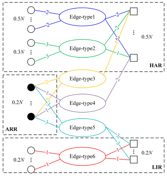
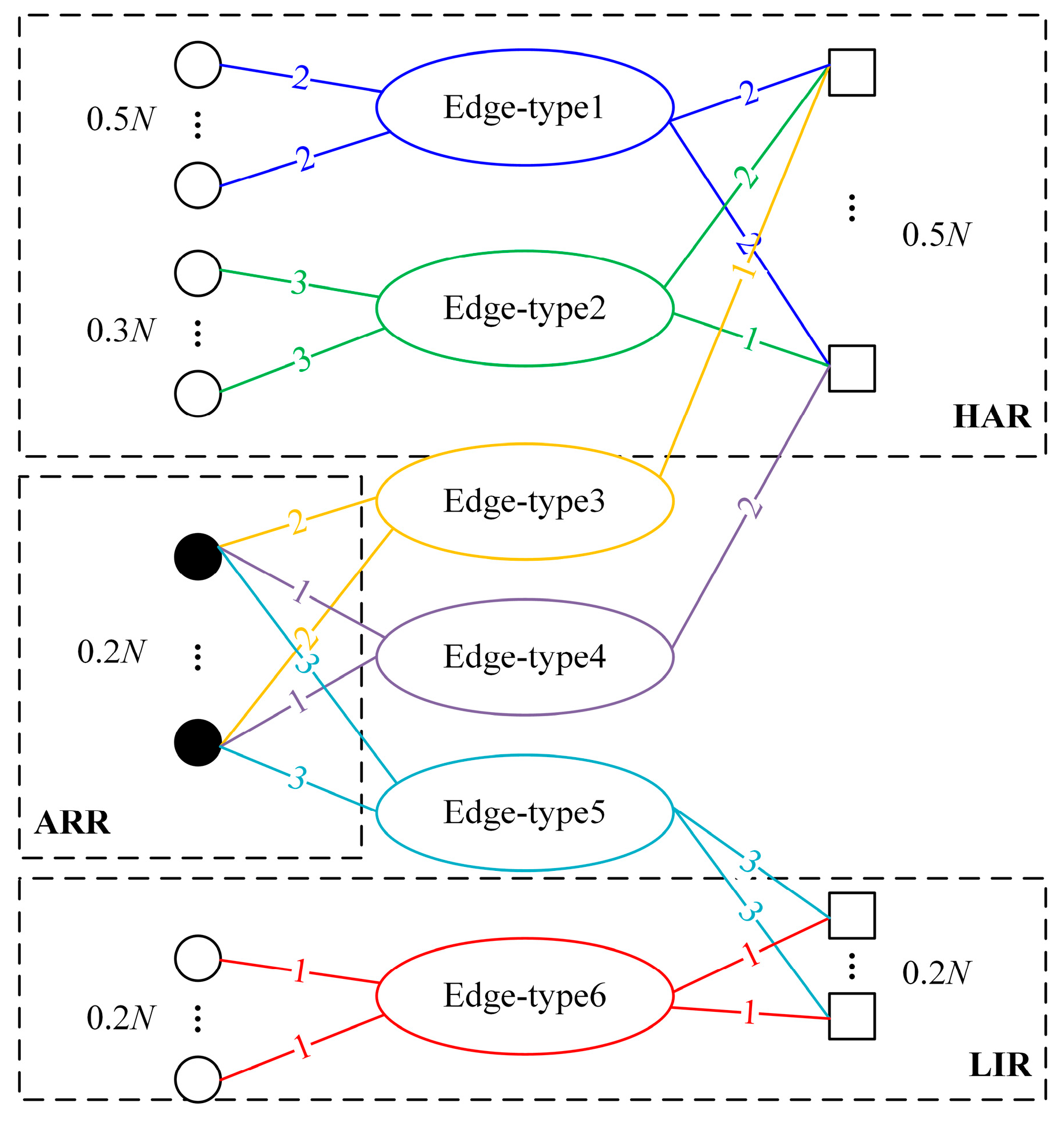
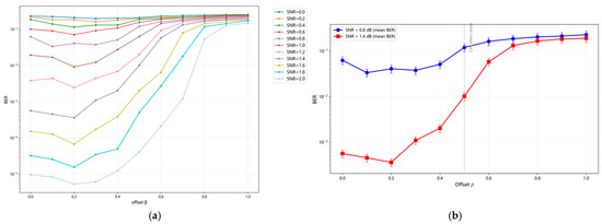
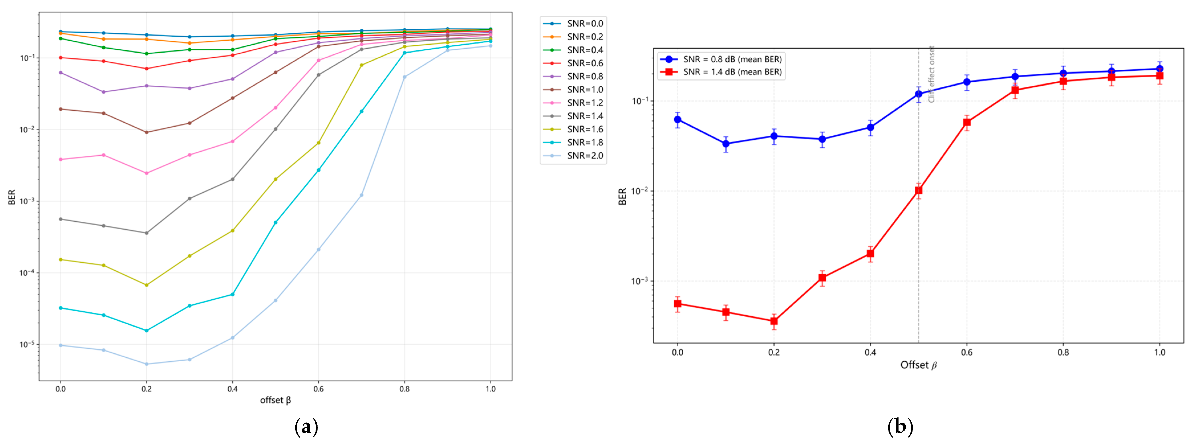
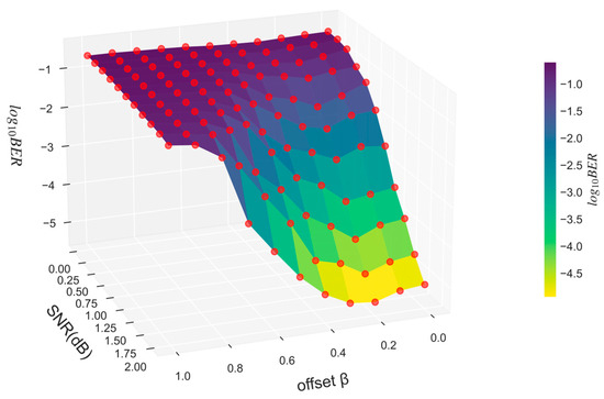
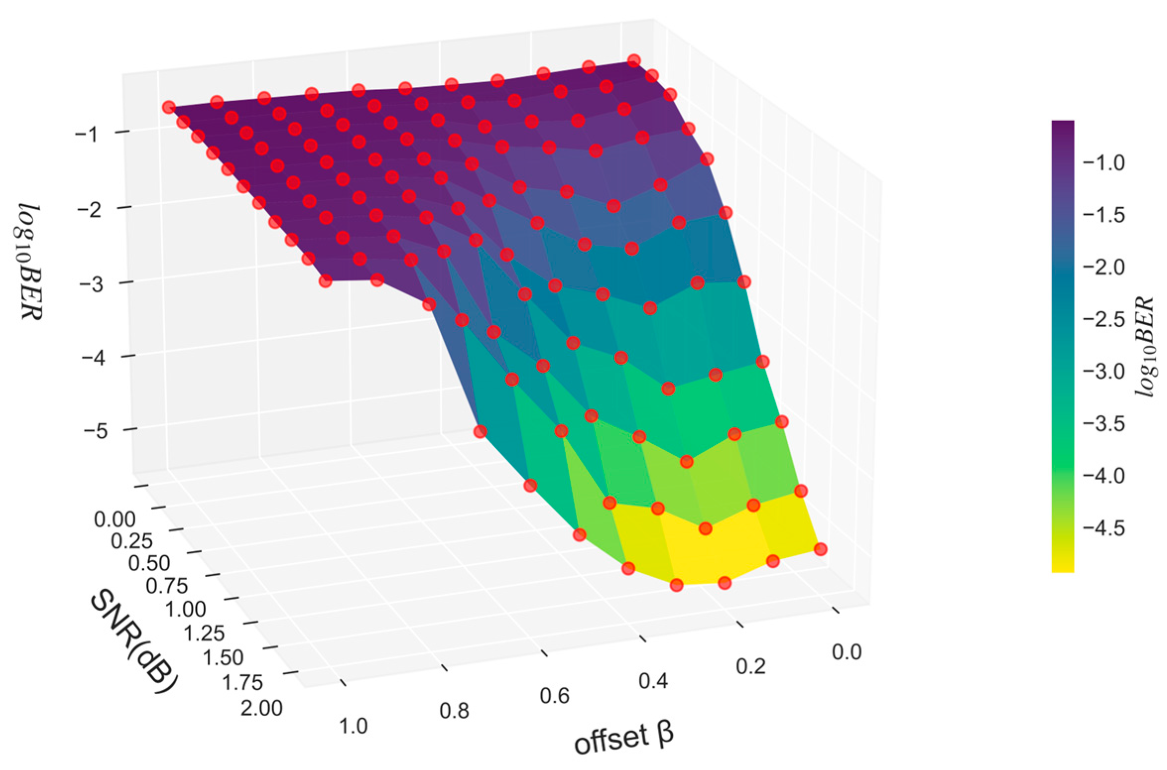
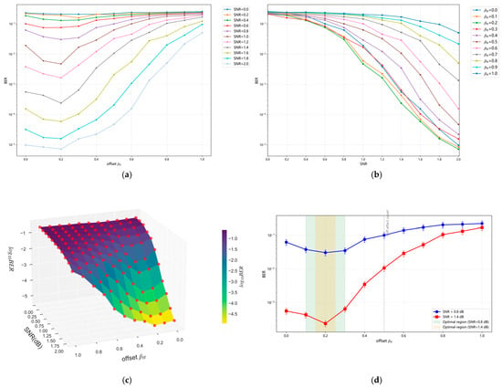
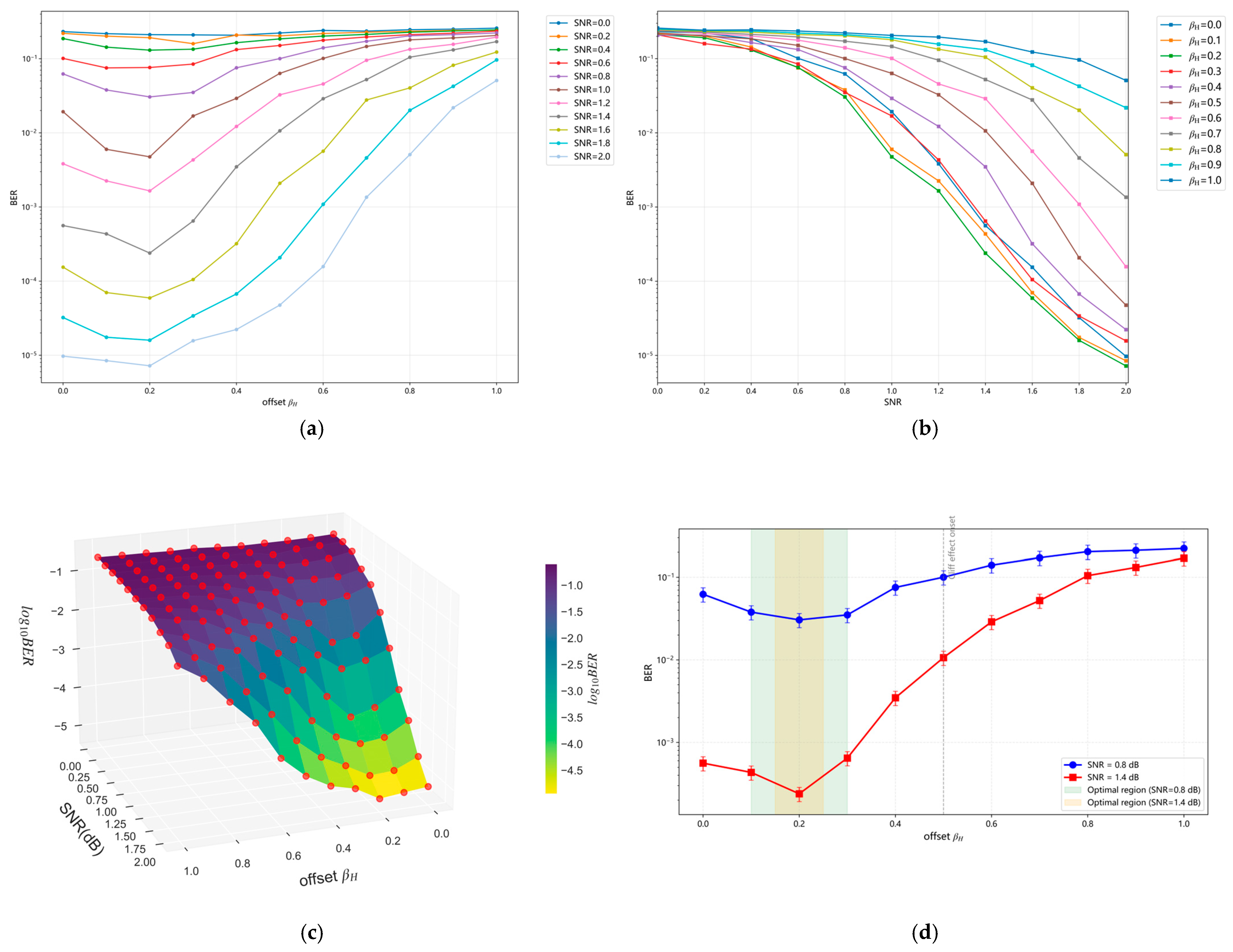
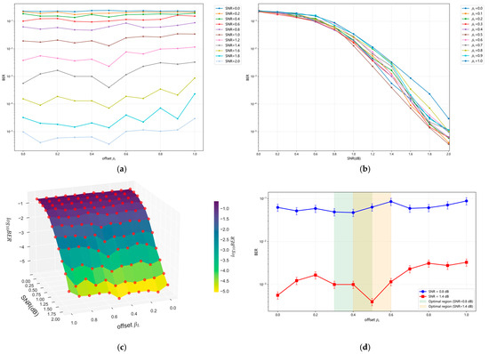
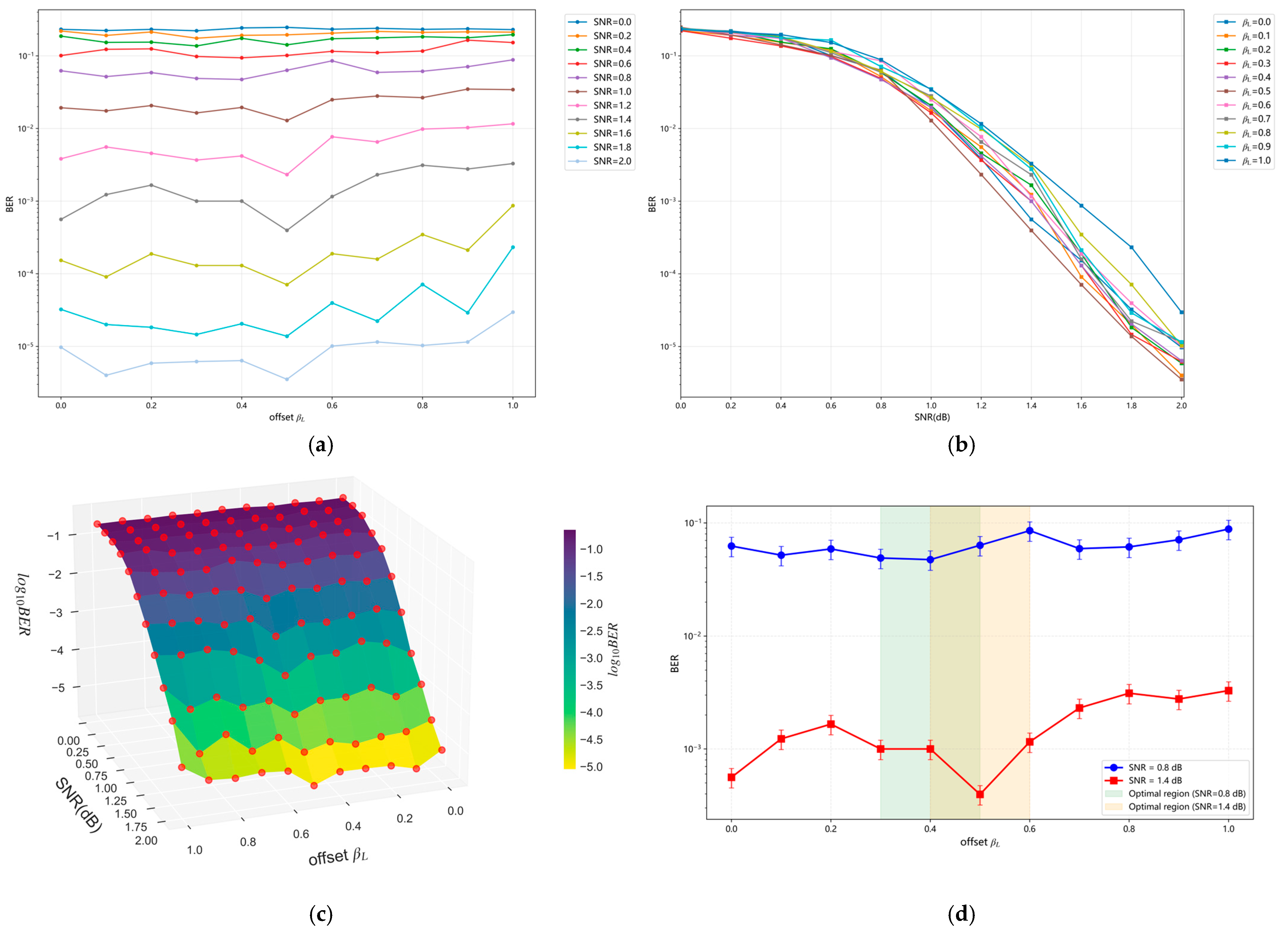
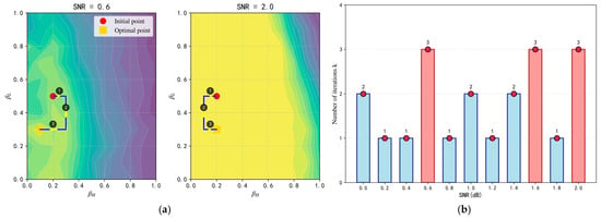
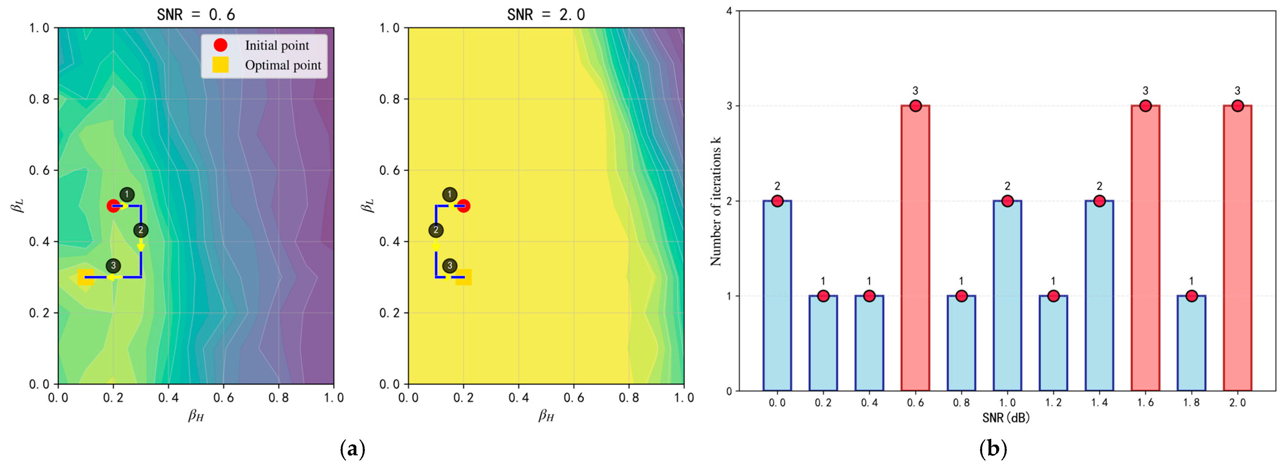
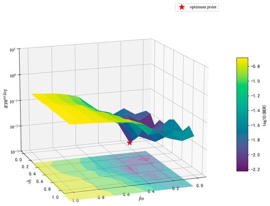
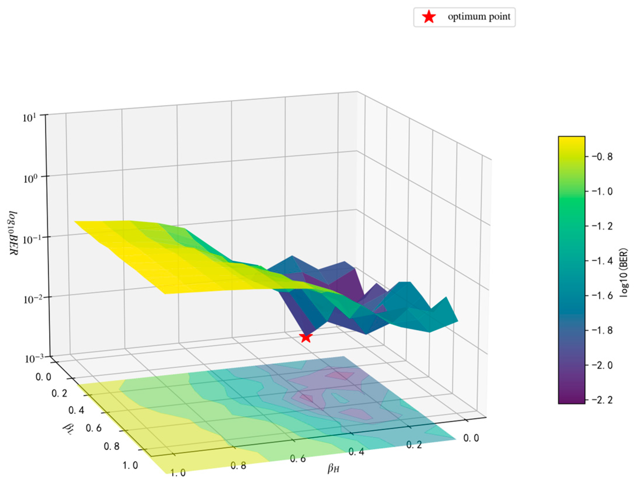
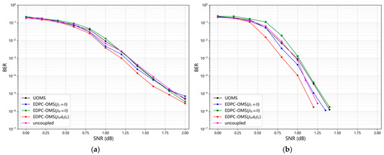
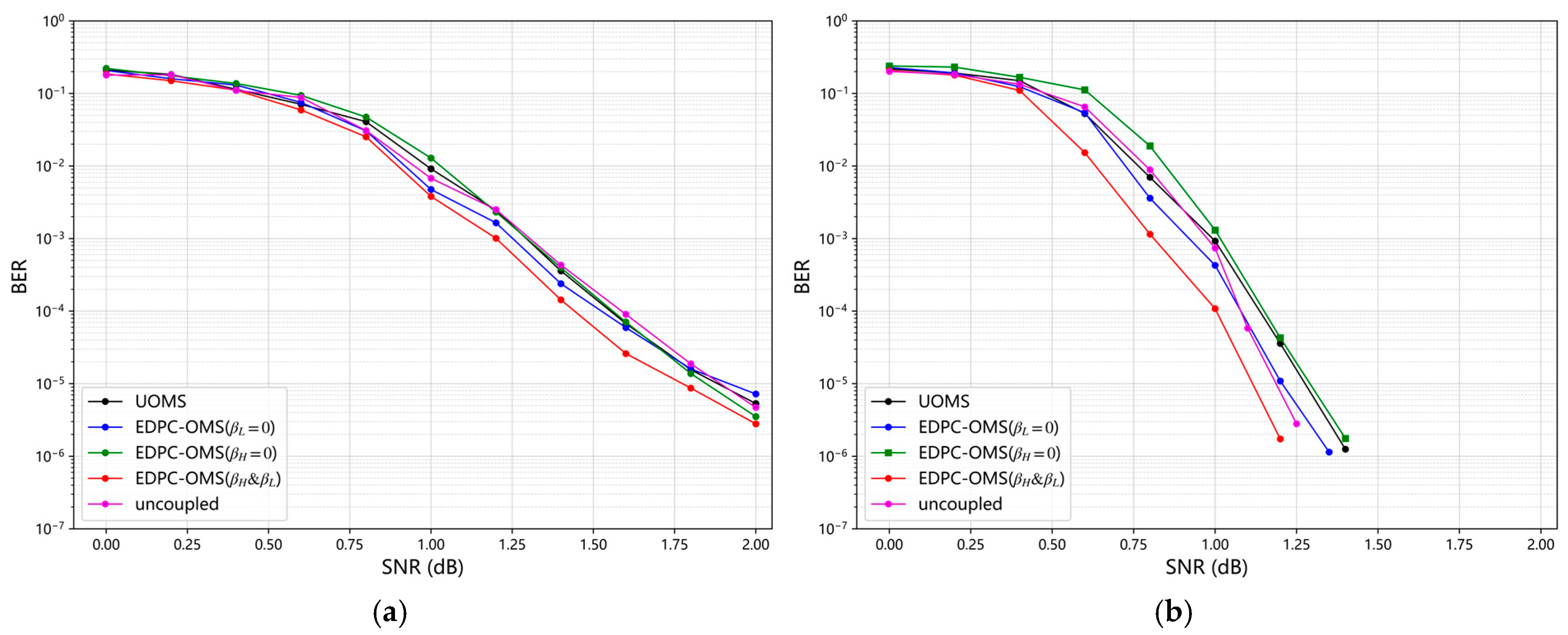
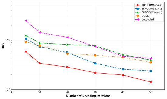
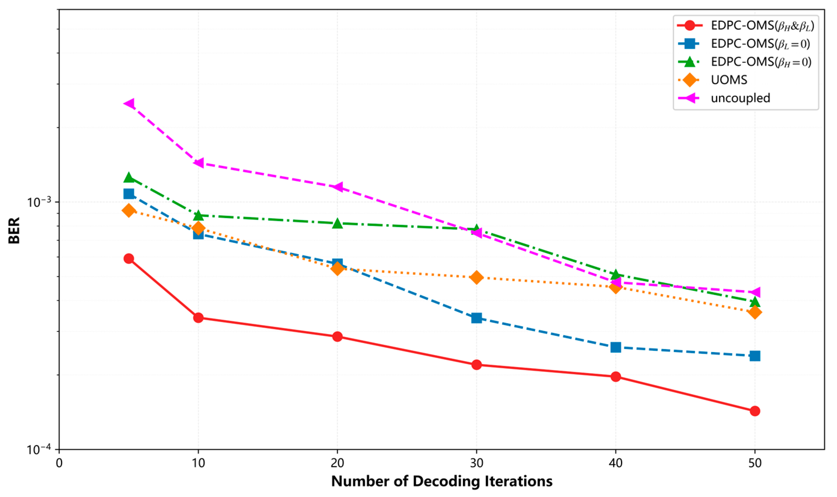
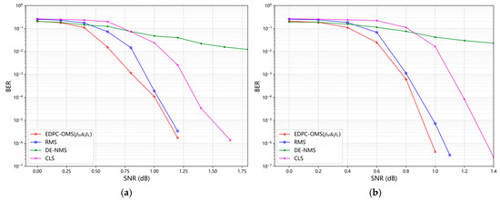
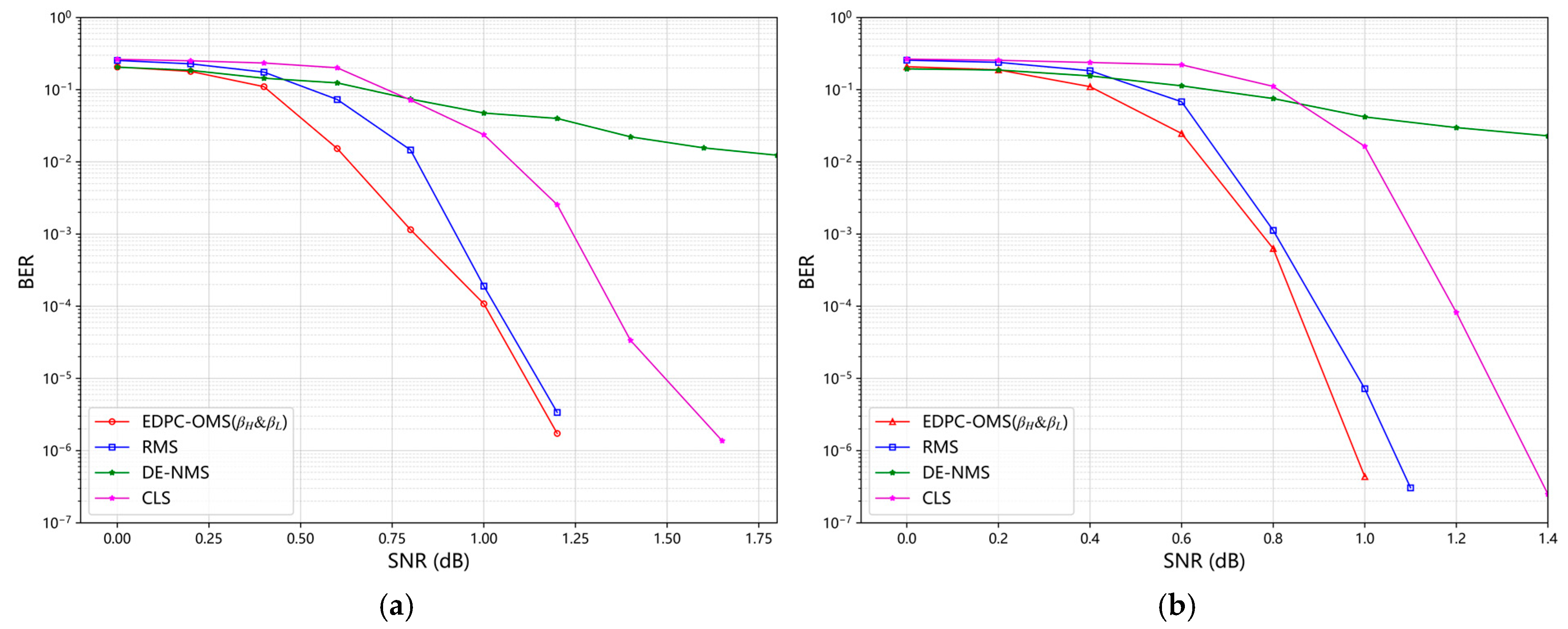
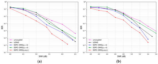
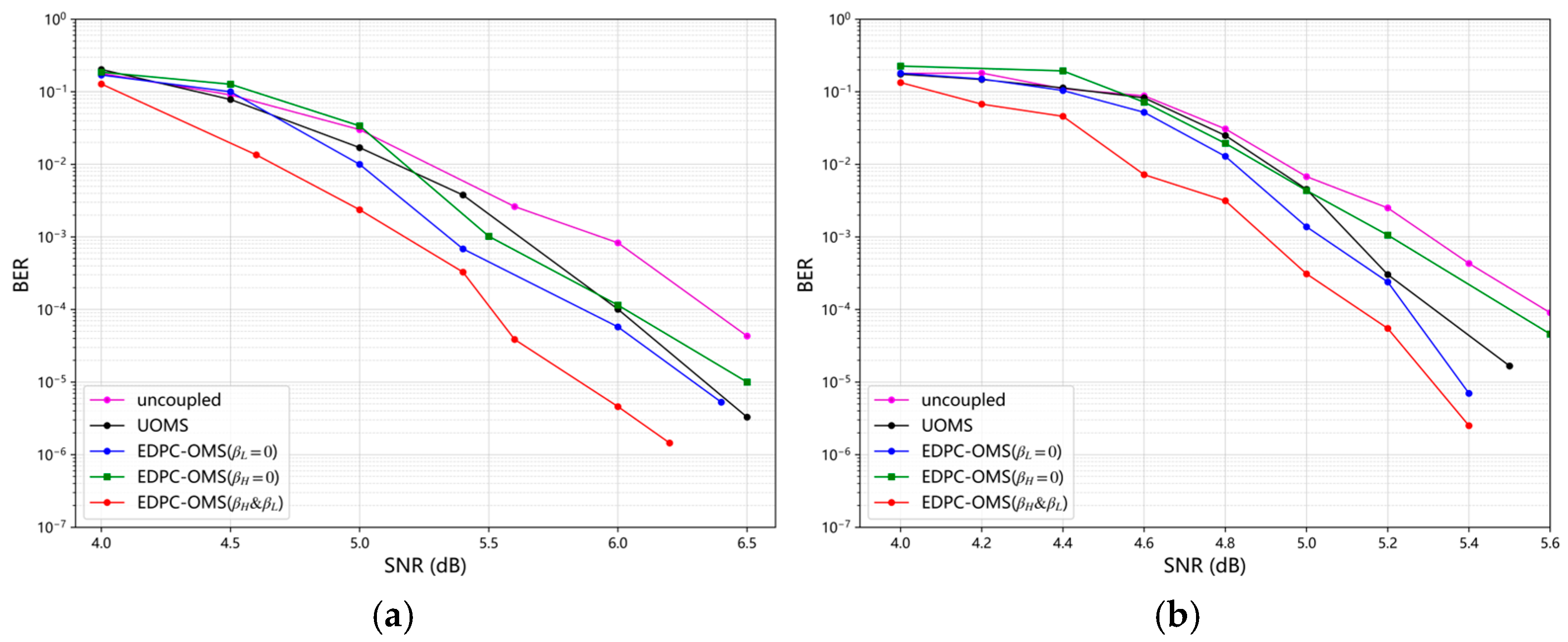
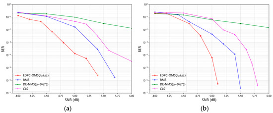
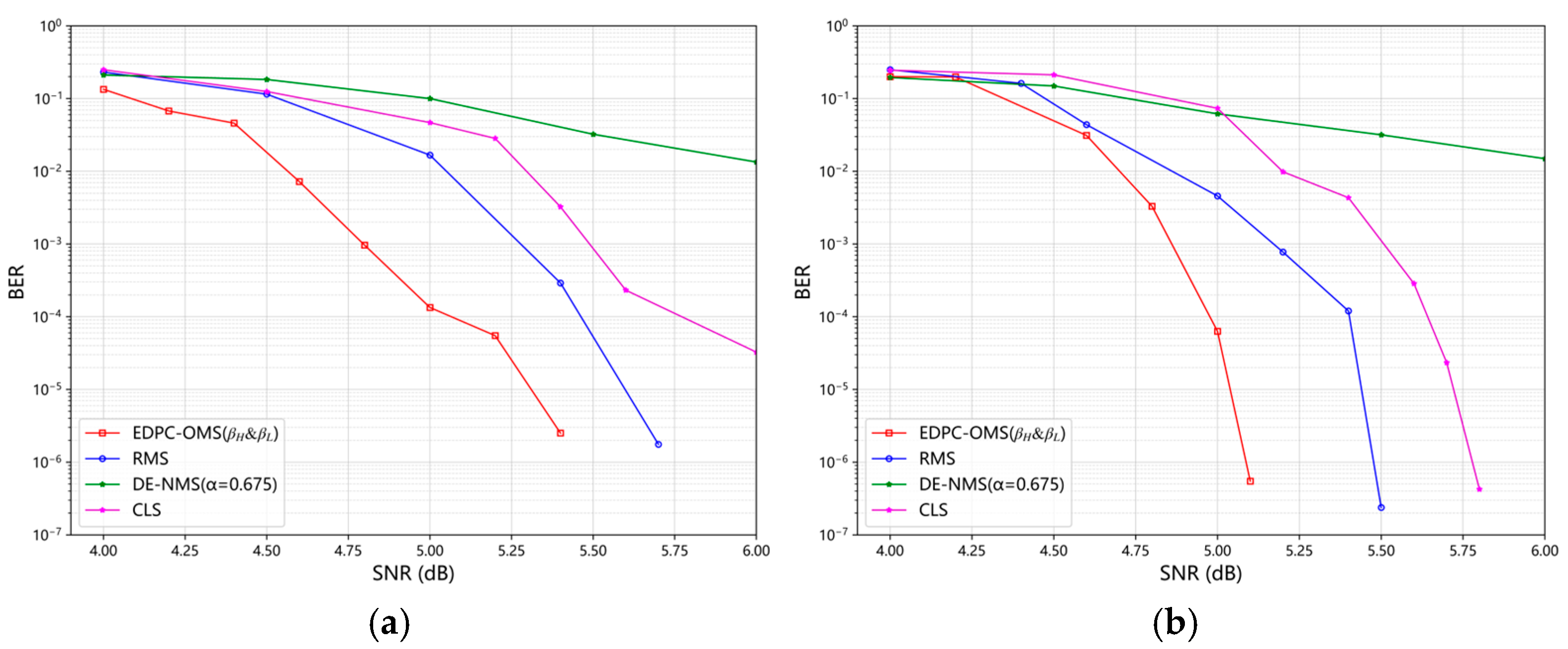

Disclaimer/Publisher’s Note: The statements, opinions and data contained in all publications are solely those of the individual author(s) and contributor(s) and not of MDPI and/or the editor(s). MDPI and/or the editor(s) disclaim responsibility for any injury to people or property resulting from any ideas, methods, instructions or products referred to in the content. |
© 2026 by the authors. Licensee MDPI, Basel, Switzerland. This article is an open access article distributed under the terms and conditions of the Creative Commons Attribution (CC BY) license.