


Abstract
Different methodologies have been developed for the analysis and study of dynamical systems, including both theoretical models and natural systems. Examples span a wide range of applications, such as astronomy, financial and economic time series, biophysical systems, physiological phenomena, and Earth sciences, including seismicity and climatic processes. The study of these complex systems is commonly based on the analysis of the signals they generate, using mathematical tools to extract relevant information. A broad spectrum of mathematical disciplines converges in this context, including stochastic, probability and statistical theory, entropic and informational measures, fractal and multifractal analysis, natural time analysis, modeling of non-linearity and recurrence methods, generalized entropies, non-extensive systems, machine learning, and high-dimensional and multivariate complexity. Research in this area is largely focused on the characterization of complex systems, providing indicators of determinism or stochasticity, distinguishing between regularity, chaos, and noise, and identifying topological as well as disorder-regularity features. In addition, short- and long-term forecasting, together with the identification of short- and long-range correlations, play a central role in such characterization. To address these objectives, numerous mathematical tools have been developed for the analysis of time series and point processes, each designed to capture specific signal properties. In this work, many of the most important tools used in time series analysis are compiled and reviewed, highlighting their main characteristics and the different types of complex systems to which they have been applied.
Keywords:
time series analysis; complex systems; dynamical systems; signal analysis; stochastic and point processes; recurrence analysis; entropy measures; fractal and multifractal analysis MSC:
37M10
1. Introduction
The study of complex systems has become a cornerstone of modern scientific inquiry, transcending traditional disciplinary boundaries to address phenomena in fields as diverse as finance, physiology, biophysics, geophysics, oceanography, atmospheric science, soil science, environmental science, and astronomy among many others. These systems are frequently characterized by intricate, non-linear dynamics that produce signals (time series) containing rich information about the underlying governing processes. However, the inherent complexity of these signals—very frequently manifesting as non-stationarity, noise, and multiscale structures—necessitates the application of a diverse and sophisticated mathematical toolkit to distinguish between determinism, stochasticity, and pure randomness. Much of the contemporary research in this domain focuses on the characterization of these systems to provide reliable indicators of regularity versus chaos.
Traditionally, the analysis of time series has relied heavily on the assumption of stationarity, i.e., the idea that statistical properties remain invariant over time. Conventional stochastic processes, where variables are indexed by a temporal parameter, provided the initial framework for understanding these dynamics [1,2]. In this context, weakly stationary processes, characterized by time-invariant means and covariance structures, allowed for the development of foundational tools like auto-correlation functions. Yet, as researchers began to explore natural systems more deeply, it became evident that many processes exhibit “memory” properties that standard models were not able to capture [3]. Short-range dependence, where correlations decay exponentially, is often superseded in complex systems by long-range dependence, where auto-correlations follow a power-law decay [4]. This persistence or anti-persistence is a fundamental feature of complex temporal dynamics.
A pivotal breakthrough in quantifying these long-range dependencies was the introduction of the Hurst exponent (H) [5]. Originally derived from hydrological studies of the Nile River, the Hurst exponent provides a measure of self-similarity and scaling behavior in time series. When , the system behaves like a random walk. However, values deviating from this value indicate either persistence () or anti-persistence (). While H provides a global characterization, it is often insufficient for real-world data that exhibit heterogeneous scaling across different segments. This led to the development of fractal and multifractal geometries, which offer a mathematical framework for describing irregular structures that look similar at different scales [6,7,8,9,10]. For example, monofractal processes, like fractional Brownian motion, are governed by a single scaling exponent, whereas multifractal processes require a spectrum of exponents to fully describe their local scaling variations [11].
To address the challenges of non-stationarity and external trends in empirical data, Detrended Fluctuation Analysis (DFA) was further developed as a robust alternative to classical power spectral analysis [12,13]. Unlike classical power spectral analysis, DFA can reliably detect intrinsic scaling properties by systematically removing polynomial trends. This method has been further extended into Multifractal DFA (MF-DFA), allowing for the characterization of multiple scaling exponents and deeper insights into system complexity [14,15]. Recent innovations in this area have even incorporated adaptive techniques like Ensemble Empirical Mode Decomposition (EEMD) to improve robustness in specific applications, such as meteorological and/or seismic data analysis.
Beyond scaling and fractals, the concept of entropy has emerged as a vital tool for measuring the complexity and uncertainty of dynamical systems [16]. Information-theoretic approaches, such as the Fisher–Shannon framework, provide complementary views of the probability distribution of a signal [17,18]. In particular, Shannon entropy quantifies global uncertainty, while the Fisher information measure (FIM) reflects local fine-scale structures. In many biological and physical systems, complexity is not just a feature of a single scale but is distributed across multiple resolutions. Multiscale entropy (MSE) was then introduced to address this, revealing that healthy physiological systems often show higher entropy (complexity) at larger scales compared to pathological ones.
In addition to the previous methodologies, natural time analysis (NTA) has emerged as a powerful framework for identifying the approach of a complex system to a critical point [19,20]. Unlike traditional analysis that treats time as a continuous or clocked parameter, natural time (denoted as ) views the system as a sequence of events, where the index serves as the temporal variable for the kth event in a series of N total events. This domain is particularly useful for analyzing point processes such as seismicity, where the occurrence of events—rather than the elapsed time between them—carries the primary dynamical information. The primary strength of natural time analysis lies in its ability to extract hidden properties of the evolution of a system through complexity measures based on entropy. For example, the entropy in natural time, S, and the entropy under time reversal, , provide unique indicators of the proximity of the system to a critical state [21,22,23,24]. This has led to successful applications in diverse fields, including the identification of sudden cardiac death risk through electrocardiogram analysis and the study of flux avalanches in superconductors. By focusing on the order and energy of events rather than their conventional timing, natural time analysis provides a scale-invariant perspective that complements fractal and multiscale methodologies.
When time-scale localization is required, wavelet analysis offers a powerful alternative to traditional Fourier transforms [25,26]. By adapting resolution with scale—providing fine time localization at high frequencies and coarse localization at low frequencies—wavelets allow for the detection of high-frequency events and the analysis of non-stationary connectivity. Families such as the Daubechies or spline wavelets have become indispensable for signal denoising and multiresolution analysis [27,28]. Furthermore, for systems where the phase space must be reconstructed from a single variable, Recurrence Plots (RPs) [29,30,31] and Recurrence Quantification Analysis (RQA) [32,33] provide a way to visualize and quantify the tendency of a system to revisit previous states. These methods, including multivariate and joint recurrence extensions, are now being integrated with machine learning to classify dynamical states and detect coupling between systems [34,35].
A critical survey of existing literature reveals a bifurcated landscape: most reviews focus either on classical statistical inference or on the burgeoning field of machine learning and deep learning. However, there is a notable scarcity of works that bridge the gap between these two extremes through the lens of complexity. This study fills that void by focusing on the “middle ground”, methodologies such as fractal analysis, recurrence quantification, and information-theoretic measures. These tools are uniquely equipped to handle the non-linear and non-stationary signatures of complex systems, providing a unified framework that connects traditional stochastic foundations with modern computational analysis.
1.1. Categorization of Methodologies
To provide a coherent synthesis, the tools discussed in this review are categorized into four primary conceptual frameworks based on the specific features of the dynamical system they aim to quantify:
- Scaling-Based Approaches (Section 2): These methods, including fractal analysis, DFA, and MF-DFA, originate from statistical physics and the study of critical phenomena. Their primary role is to characterize the “memory” and self-similarity of a signal across different scales, identifying whether a system is governed by long-range correlations or power-law scaling laws.
- Information-Theoretic Measures (Section 3): Rooted in Shannon’s communication theory and statistical mechanics, these measures (such as Shannon entropy and Fisher information) focus on the degree of uncertainty, disorder, and information “cost” of the system’s dynamics.
- Non-linear Dynamical and Geometric Methods (Section 4 and Section 6): These approaches, including RPs, RQA, and NTA, treat the signal as a trajectory in an embedded phase space. They aim to identify deterministic structures, hidden periodicities, and transitions in the system’s topology that are often invisible to linear or purely statistical methods.
- Time-Frequency and Multiresolution Frameworks (Section 5): Represented primarily by wavelet transforms, this framework transcends the limitations of traditional Fourier analysis by providing simultaneous localization in both time and frequency domains. Its role is to detect transient phenomena, non-periodic oscillations, and the evolution of spectral content over time, which is crucial for systems with shifting dynamical regimes.
A visual roadmap for the reader synthesizing the above categorization is given in Table 1.
Table 1.
Classification of methodologies by conceptual framework.
1.2. Scope and Selection Criteria
The mathematical tools compiled in this review are not chosen exhaustively, but rather through a systematic selection process aimed at providing a comprehensive “analytical workflow” for complex time series. The criteria for including the specific methodologies categorized in Section 1.1 are based on the following requirements:
- Non-stationarity Handling: Since empirical time series (geophysical, biological, or astrophysical) rarely satisfy the requirement of stationarity, methods like DFA and wavelet analysis are selected specifically for their ability to decouple local trends from long-range correlations.
- Multi-dimensional Complexity: The Fisher–Shannon framework and MF-DFA analysis are included because they provide a dual perspective on complexity, measuring both global disorder and the heterogeneity of local scaling, which single-metric approaches (like standard variance or Shannon entropy) fail to capture.
- Predictive Capability for Criticality: A primary goal of this review is to highlight tools that identify precursors to extreme events. NTA is selected due to its unique ability to reveal the approach to a critical state (e.g., solar flares or earthquakes) by transforming the time domain into a sequential event-based framework.
- Algorithmic Maturity and Implementation: We prioritize methods that have matured significantly over the last two decades and for which robust algorithmic implementations exist, ensuring that this review serves as a practical handbook for researchers.
A visual synthesis of the selection criteria is provided in Table 2.
Table 2.
Systematic selection criteria and the corresponding methodologies included in this review.
1.3. Comparative Synthesis of Time Series Methodologies
The selection of an appropriate analytical tool is rarely a matter of finding a “superior” method, but rather finding the best match for the data constraints. As shown in Table 3, while DFA is the gold standard for long, non-stationary sequences, its reliance on large datasets makes it unsuitable for the short-duration transients often found in X-ray bursts, where RQA or wavelets provide better resolution. A truly comprehensive synthesis of a complex system often requires a multi-method approach—for example, using NTA to find the “when” (criticality) and MF-DFA to find the “how” (scaling heterogeneity).
Table 3.
Comparative synthesis of time series methodologies: Data requirements, strengths, and primary constraints.
1.4. A Brief Comment on the Evolution of Time Series Analysis
While traditional time series analysis, rooted in the Box–Jenkins framework [36], primarily addresses linear and stationary processes, many real-world systems exhibit behaviors that transcend these assumptions. This research traces the evolution from these foundational stochastic models to a modern “complexity framework”. By bridging the gap between classical statistical properties and non-linear dynamics, this review provides a comprehensive map of tools designed for systems where stationarity and linearity are the exception rather than the rule.
This work is organized as follows. Section 2 establishes a preliminary background on the theoretical foundation and key concepts for understanding the analysis of complex time series. FIM theory is given in Section 3, while Section 4 describes the method of NTA along with the concepts of entropy and complexity measures in natural time. Wavelets, the modeling of non-linearity, and RPs are discussed in Section 5 and Section 6, respectively. In all these sections, modern applications to physiology, finance, and the geosciences, with a focus in seismicity, are briefly described to highlight how these tools converge to provide a unified framework for understanding the inherent richness of complex time series. Section 7 deals with a brief account of the machine learning revolution and prediction problem, while Section 8 covers the subject of high-dimensional and multivariate complexity. The overview ends in Section 9 with an account on recent applications of time series analysis to astrophysical data, while Section 10 contains the relevant conclusions along with the challenges and future directions.
2. Preliminary Background
This section provides the essential theoretical foundation for understanding the analysis of complex time series. We introduce key concepts that range from basic stochastic processes to advanced multifractal and multiscale analysis techniques that form the backbone of the modern methodology of time series.
2.1. Evolution of Time Series Analysis
The mathematical treatment of time series has evolved significantly over the last half-century. Initially, the field was dominated by the Auto-Regressive Integrated Moving Average (ARIMA) models, which rely on the assumption that a series can be transformed into a stationary state. However, as the focus of research shifted toward natural phenomena, such as seismic activity, physiological signals, and financial markets, the limitations of these “classical” models became apparent, leading to the development of the complex systems approach utilized in this research.
2.2. Stochastic Processes
A stochastic process is a collection of random variables indexed by a parameter t, which typically represents time [1]. In the context of time series analysis, the focus is primarily on discrete-time stochastic processes , where each represents the value of the process at time i. Stochastic processes exhibit fundamental properties, such as stationarity and ergodicity. In particular, stationarity is a crucial concept in time series analysis [2]. A process is said to be strictly stationary if its statistical properties remain invariant under time shifts, while it is weakly stationary (wide-sense stationarity) if its mean and covariance structure are both time-invariant, that is
However, ergodicity ensures that time averages converge to ensemble averages, allowing statistical inference from a single realization of the process. This property is important for practical time series analysis, where typically only one realization is available.
Time series can also exhibit different types of memory characteristics [3]. For instance, in cases where auto-correlations decay exponentially fast, the time series is said to have a short-range dependence. In contrast, if the auto-correlations decay as a power law, then
and the time series exhibits a long-range dependence. In fact, Equation (3) is the formal notation to indicate that an infinite series does not converge to a finite number. If negative correlations exist between past and future increments, the time series is said to be anti-persistent. These memory properties are fundamental to understanding complex temporal dynamics and form the basis for more sophisticated analysis techniques [37].
Defining Complexity: A Conceptual Framework
In the context of this study, “complexity” in time series is not merely a descriptive term for difficulty, but a formal framework characterized by four distinct pillars:
- Non-linearity: The underlying dynamics do not obey the principle of superposition, meaning small inputs can lead to disproportionately large effects.
- Non-stationarity: The statistical moments (mean, variance) evolve over time, often due to external shifts or intrinsic regime changes.
- Chaos: The system exhibits a sensitive dependence on initial conditions, making long-term deterministic prediction impossible despite the presence of underlying rules.
- Long Memory: The presence of persistent correlations where the influence of past events decays slowly (following a power law), as seen in fractal and multi-fractal processes.
Understanding these traits is essential for selecting the appropriate analytical tools discussed in subsequent sections, such as wavelets for non-stationarity or entropy for complexity quantification.
2.3. Classical Decomposition of Time Series
Before addressing the advanced measures of complexity, it is essential to consider the classical decomposition framework. Traditionally, a time series is viewed as a combination of four constituent components: (1) Trend, defined as the long-term progression of the series; (2) Seasonal, which refer to fluctuations that repeat over a fixed period (e.g., daily or annually); (3) Cyclical, referring to long-term oscillations that do not have a fixed period, often associated with economic or physical cycles; and (4) Irregular, which refers to the residual or “noise” component that remains after accounting for the previous three components.
Denoting Trend, Seasonal, Cyclical, and Irregular by , , , and , respectively, time series are typically modeled in classical analysis as additive () or multiplicative () structures. While this decomposition provides a fundamental baseline, the research in this study focuses on cases where the “Irregular” component contains complex dynamical information, such as chaos or long-range dependence, that classical methods fail to capture.
2.4. Stationarity and Diagnostic Testing
A fundamental assumption in classical time series analysis is stationarity, implying that the statistical properties of the process, such as mean and variance, do not change over time. In this research, identifying the presence or absence of stationarity is a critical diagnostic step. Two primary statistical tests are commonly employed:
- Augmented Dickey–Fuller (ADF) Test: A unit root test where the null hypothesis assumes the series is non-stationary. A low p-value suggests the series is stationary.
- Kwiatkowski–Phillips–Schmidt–Shin (KPSS) Test: Conversely, the KPSS test assumes the null hypothesis of stationarity.
Using these tests in tandem allows scientists to distinguish between series that are truly stationary, those that are unit-root non-stationary (difference-stationary), and those that exhibit deterministically changing trends. The violation of stationarity, common in the complex systems analyzed in this study, renders standard linear models like ARIMA unreliable, leading to “spurious regressions” where correlations appear significant but lack physical or causal meaning. This necessitates the use of the advanced non-linear and non-stationary tools, such as the wavelet transforms and entropy measures, discussed in later sections.
2.5. Linear Versus Non-Linear Dependency Measures
Analyzing the dependencies within and between time series is fundamental to characterizing their underlying dynamics. This research distinguishes between linear measures and those rooted in information theory. For instance, auto-correlation and cross-correlation are classical tools that measure the linear relationship between a variable and its lagged version (auto-correlation) or between two different variables (cross-correlation). While efficient for identifying seasonality and trend, they fail to detect non-linear dependencies. Based on Shannon entropy, mutual information (MI) quantifies the amount of information obtained about one random variable through the observation of another. Unlike correlation, MI does not assume linearity or a specific distribution, making it indispensable for the complex, non-linear systems analyzed in this study.
The transition from correlation-based analysis to MI allows for a more robust detection of “hidden” dependencies. In complex time series, a zero correlation does not necessarily imply independence, as the system may be governed by non-linear deterministic rules that only information-theoretic measures can reveal.
2.6. Deterministic Versus Stochastic Frameworks
A fundamental challenge in the analysis of complex signals is distinguishing between deterministic dynamics and stochastic processes. This research categorizes models based on the nature of their underlying drivers. In particular, deterministic models are systems governed by fixed rules or differential equations. While they can exhibit highly complex and unpredictable behavior (chaos) due to sensitive dependence on initial conditions, they do not contain inherent randomness. The complexity arises from the non-linear interactions within the system itself. In contrast, stochastic processes incorporate probabilistic variables and random components (noise). Traditional methods, such as the ARIMA family, assume that the irregular component of a time series is a stochastic “white noise” process.
In practice, many real-world complex time series are neither purely deterministic nor purely stochastic but represent a combination of the two. Identifying the “deterministic” versus the “stochastic” signature of a signal is crucial for selecting appropriate forecasting methods, as deterministic chaos requires state-space reconstruction techniques, whereas stochastic systems are better addressed through probabilistic modeling.
2.7. The Hurst Exponent
The Hurst exponent, H, introduced by Harold E. Hurst in his studies of the Nile River discharge [5], quantifies the long-range dependence and self-similarity properties of time series, providing a single parameter characterization of the temporal correlation structure. For a self-similar process with stationary increments, the Hurst exponent relates to the scaling behavior of the variance [11]
The Hurst exponent takes values in the interval and accepts the following interpretations depending on its value. A value signifies that the time series exhibits properties similar to a random walk or a geometric Brownian motion, implying that there is no long-term dependence or persistence in the time series. In this case, the auto-correlations decay exponentially quickly to zero, indicating a short-memory process. A value of H in the interval (0.5, 1) indicates a time series with long-term positive auto-correlation, meaning that the decay in auto-correlation is slower than exponential and follows a power law, while a value in the interval (0, 0.5) is indicative of a time series with long-term switching between high and low values in adjacent pairs, also following a power law.
Several methods exist in the literature to estimate the Hurst exponent [4]. These methods include the original method using rescaled range statistics (R/S analysis) [5], the periodogram method using the power law behavior of the spectral density, the variance-time plots based on the scaling of sample variance with the aggregation level, and DFA, which, as explained later in this section, is a robust method that removes polynomial trends [38]. In general, the choice of the estimation method affects the accuracy and computational complexity.
2.8. Fractals and Multifractals
Fractal geometry provides a mathematical framework for describing irregular, self-similar structures that appear at multiple scales [6]. In time series analysis, fractal concepts are useful for characterizing the scaling properties of temporal data. In general, a fractal can be defined as an infinitely complex geometric shape or pattern that exhibits self-similarity (that is, it looks similar at different scales) and a fractal dimension that exceeds its topological dimension. The fractal dimension, D, quantifies how a pattern fills space, and for time series, it is related to the Hurst exponent via the relation
which connects the geometric properties of the time series trajectories to its temporal correlation. While the Hurst exponent provides a single scaling parameter that characterizes the global fractal dimension of a time series, this approach assumes a uniform scaling behavior across all scales and time segments, a property which characterizes a monofractal process. Examples of monofractal processes include the fractional Brownian motion and simple self-similar processes [11]. However, many real-world time series, particularly in financial markets, turbulence, and physiological signals, exhibit more complex scaling behavior where different portions of the data may have different local scaling properties. These multifractal processes cannot be adequately described by a single Hurst exponent, as their scaling behavior varies locally, requiring a spectrum of scaling exponents to fully characterize their fractal structure [7]. This limitation of monofractal analysis motivates the need for multifractal methods that can capture the rich, heterogeneous scaling dynamics present in complex time series.
The multifractal formalism is based on the partition function [8]:
where represents the measure in the ith segment of size s and q is the moment order. The scaling exponent, , is defined through the proportionality expression
The multifractal spectrum, commonly denoted , is a function that characterizes the distribution of local scaling exponents (i.e., singularities) within a multifractal time series [9,10]. The spectrum plots the fractal dimension against the Hölder exponent, defined as , where each represents the local scaling behavior at different points or segments of the data [39]. The shape and width of this spectrum reveal important information about the multifractal structure. A narrow spectrum indicates a relatively uniform scaling (closer to monofractal behavior), while a broad spectrum suggests strong multifractal properties with highly heterogeneous local scaling. The maximum of usually occurs at , which corresponds to the most frequent scaling exponent in the series and is often related to the global Hurst exponent, while the asymmetric shape of the spectrum can indicate the relative prevalence of different types of scaling behavior throughout the time series.
While the scaling-based approaches discussed thus far focus on the correlation and memory of the signal, they provide limited information regarding the global disorder of the system. Section 3 introduces information-theoretic measures that complement scaling analysis by quantifying uncertainty and complexity.
2.9. Detrended Fluctuation Analysis
Detrended fluctuation analysis (DFA) is a widely used method for quantifying long-range temporal correlations in time series data, particularly those that are non-stationary. Originally developed by Peng et al. [12] for the analysis of DNA sequences, a landmark application in biophysics, DFA has since become a fundamental tool in a wide variety of fields, including physiology, economics, climatology, seismology, and neuroscience. The method addresses a critical limitation of traditional correlation analysis techniques, which often fail in the presence of external trends, drift, or other non-stationarities that are commonly found in real-world data. Unlike classical methods such as power spectral analysis or auto-correlation functions, DFA can reliably detect scaling properties and long-range correlations even when the underlying signal contains polynomial trends, seasonal variations, or other systematic non-stationarities that would otherwise mask the intrinsic correlation structure.
The theoretical foundation of DFA rests on the concept that many natural phenomena exhibit scale-invariant properties, meaning that their statistical characteristics remain similar across different time scales. This scale invariance often manifests as power-law relationships in the fluctuation characteristics, which DFA is specifically designed to detect and quantify. The DFA algorithm operates through a systematic multi-step procedure that carefully separates intrinsic scaling behavior from extrinsic trends. The process begins by first integrating the time series to convert it into a random walk-like process [38], that is
where is the mean of the series. This integrated series is then divided into non-overlapping windows each of length n, and within each window w, the local trend is removed by subtracting a polynomial fit . The size of the windows serves as a fundamental scale parameter and the order of the polynomial whether the detrending is linear (removing only constant trends), quadratic (removing linear trends), or higher-order (removing more complex systematic variations). As a final step, the detrended fluctuation for each window is calculated as follows:
and the overall fluctuation function is obtained by averaging over all windows:
where denotes an averaging procedure over all windows w. The method is robust to polynomial trends up to order , reliable for finite-size time series, and computationally efficient [13]. The power of DFA emerges when this detrending and fluctuation calculation process is repeated across multiple window sizes, typically spanning several orders of magnitude. The relationship between fluctuation magnitude and window size, when plotted on logarithmic scales, reveals the fundamental scaling behavior of the original time series through a power-law relationship. This scaling relationship encodes information about the temporal correlation structure that persists across different time scales, providing insights into the underlying dynamical processes that generate the observed data. The slope of this log–log relationship yields the scaling exponent, which serves as a quantitative measure of the strength and nature of long-range temporal correlations in the system under investigation.
2.10. Multifractal DFA
Kantelhardt et al. [14] extended the original DFA method to multifractal DFA (MF-DFA) by introducing the qth-order fluctuation function
where represents the total number of non-overlapping windows of size n that can be fit into the integrated time series. In mathematical form, for a time series of length N, where the symbol is the floor function (rounding down to the nearest integer). The MF-DFA allows for the characterization of multiple scaling exponents and provides deeper insights into the complexity of temporal correlations. Ihlen [15] gives a good introduction to MF-DFA in Matlab.
The power-law relationship reveals the scaling exponent , which characterizes the temporal correlation structure. For white noise, ; for persistent long-range correlations (i.e., pink noise), ; and for anti-persistent behavior, . The special case corresponds to noise, while represents Brownian motion. In multifractal analysis, the generalized Hurst exponent is defined through , and the singularity spectrum can be obtained via Legendre transformation: and , where is the mass exponent. When , corresponds to the standard Hurst exponent. For monofractal processes , while for multifractal processes varies with q. The degree of multifractality is quantified by the width of the spectrum, . The quantity is a measure of multifractality. The above framework has proven invaluable in biomedical applications, where altered correlation properties often reflect pathological states, as demonstrated in studies of heart rate variability [40] and brain dynamics [41].
Recent modifications of the MF-DFA approach have been proposed to improve its robustness and applicability to specific types of data [42,43]. The main mathematical innovation is replacing the discontinuous polynomial detrending with EEMD-based trend extraction and using overlapping windows instead of non-overlapping segments to better preserve the continuity of the time series and reduce pseudo-fluctuation errors. For example, Zhang et al. [42] apply the modified MF-DFA specifically to analyze precipitation data in the Dongting Lake Basin in China. They examine the multifractal characteristics of rainfall in this particular geographic region, likely to understand local precipitation patterns, variability, and scaling behaviors that could inform water resource management and flood prediction in this important lake basin, while Morales Martínez et al. [43] provide a more methodological paper that develops or refines the modified MF-DFA approach for precipitation analysis more generally. Rather than focusing on a specific geographic location, they seem to be advancing the analytical technique itself, potentially making it more robust or applicable for studying precipitation multifractal properties across different contexts. Two studies that highlight the contemporary relevance of DFA and MF-DFA in molecular biophysics are reported by Yu et al. [44] and Rosas et al. [45]. In particular, Yu et al. [44] introduces a time series model where DNA nucleotides (A, C, G, T) are mapped to numerical values (e.g., , , , ) to be analyzed statistically, where multifractal analysis is used to provide a dimension spectrum to more comprehensively discuss the complex patterns in DNA. A multifractal analysis on DNA walks and trails is carried out by Rosas et al. [45], where DFA is used to eliminate local trends (biases in nucleotide composition) to reveal the true long-range fractal properties of the sequence and MF-DFA is employed to determine whether a sequence is monofractal (i.e., characterized by a single scaling exponent) or multifractal (i.e., characterized by multiple exponents). Both works aim to distinguish between coding and noncoding regions and identify long-range correlations due to patterns that repeat or persist over thousands of nucleotides which are invisible to standard linear statistical methods.
2.11. Multiscale Analysis
Multiscale analysis is a fundamental approach in time series analysis that examines data across multiple temporal scales to reveal complex patterns and structures that may be hidden when viewing data at a single resolution. This methodology recognizes that many natural and artificial systems exhibit a behavior that varies dramatically depending on the time scale of observation. For example, phenomena that appear random or chaotic at short time scales may reveal clear trends or periodic patterns when examined over longer periods, and vice versa.
The theoretical foundation of multiscale analysis rests on the concept that complex systems often exhibit scale-invariant or self-similar properties, where statistical characteristics remain consistent across different temporal resolutions. This is particularly relevant in fields such as hydrology, climatology, finance, and geophysics, where time-series data may contain information that spans multiple orders of magnitude in time (i.e., from seconds to decades). Traditional single-scale analysis methods can miss critical information embedded at different temporal scales, potentially leading to incomplete or misleading interpretations of the underlying dynamics of the system.
The multiscale entropy (MSE), introduced by Costa et al. [16] and further developed by Costa et al. [46], quantifies the complexity of time series across multiple temporal scales by calculating the sample entropy at different coarse-grained versions of the original data. The method robustly separates healthy and pathologic groups and consistently yields higher values for simulated long-range correlated noise compared to uncorrelated noise. The coarse-graining procedure creates new time series, , from the original series, , such that
for , where is a scale factor. For each coarse-grained series, the Sample Entropy is calculated as [47]
where A is the number of template matches of length , B is the number of template matches of length m, and r is the tolerance for matching. The MSE is then defined as the sample entropy calculated for each scale
This approach reveals that many physiological and complex systems show increasing entropy at larger scales, indicating the presence of long-range correlations and structured variability that appears as complexity rather than mere randomness. For example, a healthy heart rate variability typically shows higher multiscale entropy compared to pathological conditions, where the complexity is reduced across multiple scales.
Recent developments have expanded the multiscale analysis toolkit with several sophisticated approaches. For example, the empirical mode decomposition (EMD), developed by Huang et al. [48], adaptively decomposes a time series into intrinsic mode functions (IMFs) without requiring a priori assumptions about the data structure. The improved EEMD, as was used in the study by Zhang et al. [42] that was mentioned earlier, addresses mode mixing issues by adding white noise to the decomposition process. Other advanced multiscale methods include the Multiscale Principal Component Analysis (MSPCA), which combines wavelet decomposition with PCA to identify dominant patterns at different scales [49,50], while the Multiscale Network Analysis examines how correlation structures evolve across temporal scales, revealing scale-dependent connectivity patterns in complex systems [51,52,53].
The power of multiscale analysis lies in its ability to bridge the gap between microscopic fluctuations and macroscopic behavior, providing a more complete understanding of complex systems. By examining how statistical properties, correlations, and patterns evolve across different time scales, scientists can identify the dominant processes governing system behavior, predict future states more accurately, and develop more robust models that capture the full richness of temporal dynamics present in real-world data [54]. This comprehensive approach has become indispensable for understanding the inherently multiscale nature of complex systems across diverse scientific disciplines.
3. Fisher–Shannon Information Theory
In recent years, the Fisher–Shannon information framework has emerged as a valuable tool for quantifying the complexity and non-stationary behavior of non-linear time series.
Let X be a random variable with probability density function . FIM and Shannon entropy associated with X are defined, respectively, as
FIM and Shannon entropy are complementary quantities, each exhibiting distinct properties, quantifying, respectively, the sharpness of the probability distribution, and the uncertainty associated with the random variable’s outcomes. As discussed by Rosso et al. [17], the Shannon entropy can be understood as a measure of the distribution’s global characteristics, remaining largely unaffected by substantial variations in the distribution. In contrast, FIM is interpreted as a measure of the distribution’s local features, reflecting the capacity to accurately model its fine-scale structure.
For analytical convenience, the Shannon entropy is often expressed in terms of the entropy power, defined as [18]
Among several properties, both measures and verify a set of resembling inequalities [55]:
- Evolution law: if X represents the state of a system, the second law of thermodynamics implies thatwhereas the I-theorem becomes, accordingly,
- Super-additivity property: the Shannon entropy of the sum of two independent random variables satisfies both the entropy power inequality [56]and the Fisher information inequality
- Scaling property: the entropy power and the FIM of a random variable X scaled by a factor are
- Uncertainty property:with equality if and only if X is a Gaussian random variable. This inequality was demonstrated by Dembo et al. [56], and indicates that FIM and are strongly connected.
3.1. Some Analytical Formulae for Fisher Information Measure and Shannon Entropy Power
This subsection reports analytical expressions for the Shannon entropy power and the FIM for several parametric probability distributions, which can be directly applied to parametric estimation problems. These expressions were first demonstrated by Lazo and Rathie [57], Vignat and Bercher [55], and Guignard et al. [58].
- The Student-t distribution: the probability density function of a Student-t random variable with parameters m and is given by:whereand is a scale parameter. The Gaussian distribution can be recovered from the Student-t family by taking the limits or .The Shannon entropy power and FIM are, respectively,where is the digamma function.
- The power exponential distribution: The probability density function of a power exponential random variable x with parameters , is given by:where is a scale parameter and is a shape parameter. Note that corresponds to the Gaussian case, while yields a uniform distribution. This versatility makes these distributions particularly suitable for precisely modeling physically relevant quantities as, for example, the amplitudes of wavelet coefficients. In addition, it has been demonstrated that they achieve the maximum Shannon entropy under a constraint on the moments [59].The Shannon entropy power and the FIM of the power exponential law with parameters and are
- The Gamma distribution: The probability density function of a Gamma random variable x with parameters is given bywhere denotes the Gamma function and are the scale and shape parameters, respectively.The Shannon Entropy Power iswhere is the digamma function.The FIM iswhere the restriction must hold in order to ensure convergence and be physically meaningful.
- The Weibull distribution: The probability density function of a Weibull random variable x with parameters , , and is given bywhere is the location parameter, is the scale parameter, and is the shape parameter.The Shannon entropy power of the Weibull distribution is given bywhereand denotes the Euler–Mascheroni constant, while the FIM isSubstitution of into Equation (34) gives, for the argument of the Gamma function, , which must remain strictly positive for the integral to converge. Therefore, the FIM is only valid for shape parameters .
- The log-normal distribution: The probability density function of a log-normal random variable x with parameters and is given bywhere the parameters and are defined such that the logarithm of a log-normal random variable follows a normal distribution with mean and variance .The Shannon entropy power and the FIM are given byrespectively.
3.2. The Fisher–Shannon Information Plane
The distribution of a variable X can be analyzed within the so-called Fisher–Shannon Information Plane (FSIP), a representation space whose coordinates are given by the FIM and the Shannon entropy power. In the FSIP, the attainable values are confined to the domain
as imposed by the inequality . Vignat and Bercher [55] demonstrated that for any point , there exists a random variable X—distributed according to an exponential power law—such that and . The product is also called complexity, and a curve in is iso-complex if remains constant along the curve. Due to the scaling property, the complexity of a variable X is constant up to a multiplicative factor , and thus varying a one can move along any iso-complex curve.
The boundary of corresponds to the iso-complex curve for which , attained if and only if X is Gaussian. On this boundary, the standard deviation —which plays the role of the scaling parameter in the Gaussian case—is equivalent to the multiplicative factor a.
In practical applications involving empirical time series, the underlying probability density function is generally unknown and must be estimated from the discrete data samples . While simple histograms can provide a rough estimate of the distribution for Shannon entropy, the calculation of Fisher information, which involves the gradient of the density, requires a smooth and differentiable estimate. Consequently, the so-called Kernel Density Estimation (KDE) is typically employed [60]. In KDE, the density is estimated as:
where K is a smooth kernel function (often Gaussian) and h is the bandwidth. The choice of h is crucial; a bandwidth that is too small introduces noise into the Fisher information calculation, while one that is too large may obscure the local gradients that the measure is intended to capture. Common practice involves using optimized bandwidth selection rules, such as Silverman’s rule of thumb, to ensure a robust estimation of the information-theoretic plane.
Although information-theoretic planes offer a powerful global view of system complexity, they often lack temporal or frequency localization. Section 5 addresses this by introducing Wavelet transforms, which provide a multi-resolution framework for identifying where these complexities arise in the time-frequency domain. In addition, while information-theoretic measures like Shannon entropy provide a global overview of system disorder, they often lack the scale-specific detail of fractal measures (Section 2). Conversely, whereas DFA can identify long-range correlations, it cannot distinguish between different degrees of complexity within the same scaling regime. Therefore, a comparative analysis using FSIP is often superior, as it captures both local gradients and global uncertainty simultaneously.
4. Natural Time Analysis
The fundamental concept of NTA is to shift the focus from the conventional time of occurrence to the sequential order of events. By doing so, the method filters out the “noise” of varying time intervals to reveal the underlying dynamical evolution of a system as it approaches a critical state.
4.1. Natural Time
Natural Time Analysis (NTA) is a statistical method used to study complex systems and critical phenomena through the analysis of time series. Rather than using conventional or clock time, this tool measures time using sequences of events (fluctuations in a physical observable). The concept of natural time was introduced in 2001 by Varotsos et al. [19] to study seismic electrical signals (SESs), which were observed before large earthquakes [20]. These SESs were defined as transient variations in the Earth’s electric field, which were recorded as fluctuations in the self-electric potential that was measured directly from the ground. NTA has been applied to diverse complex systems as self-organizing critical systems (SOC). In this line, Bak et al. [21,22] introduced the sand pile model to explain many systems as, for example, the dynamics of avalanches which has allowed us to understand seismic processes, including earthquake prediction and the theoretical earthquake model proposed by Burridge and Knopoff [61].
Natural time analysis has been used in experiments to diagnose heart failure syndrome [62,63,64]. In particular, the methodology proposed by Varotsos et al. [65] enables the identification of patients at elevated risk of sudden cardiac death, even when only heart rate is monitored, via electrocardiography or through substantially more cost-effective and portable devices. Moreover, analogous methodological applications have been demonstrated in the context of financial markets [66].
Natural time, denoted as , is defined as
where N denotes the total number of events in the temporal data sequence and k labels the position of the event within this sequence, i.e., it is the index of the kth event, with .
A time series consists of a sequence of values, , of some measurable physical quantity sampled at regular time intervals, whereas a point process is observed at irregular time intervals, as in the case of earthquake catalogs. NTA can be applied to both types of data because only the ordering of the values is relevant. Consequently, the natural time introduces a new, non-continuous time domain whose values form a countable set (see Figure 1).
Figure 1.
(a) Example of point processes in conventional time and (b) as they appear in NTA. The black frames in both plots indicate the length of the window, while the arrows are depicted to provide a comparison of the temporal separation distance between consecutive events in real and natural time.
To describe the evolution of the process under study, pairs of the form are considered, where typically represents a quantity proportional to the energy released in the individual kth event. However, the analysis becomes more tractable if the pairs are transformed into , where defined as
is the probability of the occurrence of the kth event, which must satisfy the condition
It is well known from probability theory that the characteristic function of a random variable allows us to describe the properties and behavior of their probability distribution. Let X be a random variable with probability distribution F. The characteristic function of F (or X) is the function defined for all t as
For distributions F with a probability distribution function f, the function obeys the expression
where is referred to as the Fourier–Stieltjes transform of F.
In NTA, the characteristic function of is defined for all as:
where and is the natural frequency. The normalized power spectrum is defined by the formula
It is also known from probability theory that if all moments of X are finite, then the characteristic function can be calculated by expanding the complex exponential function in its power series. Thus, the moments of the distribution are calculated from the behavior of the characteristic function as . The nth derivative of the characteristic function in the limit when , i.e.,
reveals the important property that it is related to the nth moment of the distribution of , where .
4.2. Variance and Order Parameter in Natural Time
The expansion of the characteristic function, , around leads to
where
is the order parameter or second statistical moment evaluated at .
The critical state of a wide variety of complex dynamical systems, including earthquakes, is achieved when . The signals emitted by complex dynamic systems allow us to identify some of the dynamic properties of the system under study. When the system is in equilibrium, it should produce stationary time series with probability independent of . However, when a system is out of equilibrium, it is possible for the system to approach a critical state. In these phases, which are associated with the approach to a critical state, a significant increase in fluctuations is observed and long-range correlation lengths occur simultaneously [67,68,69]. When a system is out of equilibrium, it is possible for the system to approach a critical state. As a consequence, the time series is non-stationary and will no longer be independent of . Another case corresponds to self-organized criticality, where NTA was applied to a set of experimental data from a critically self-organized system (SOC), such as a rice pile [70], and to the time series obtained numerically from the Burridge–Knopoff train model for earthquakes. In both cases, it is shown that converge to 0.070. Theoretical results, as obtained from the sand pile BTW model [22], indicate that avalanches are archetypical systems exhibiting self-organization. The BTW model is a multi-particle dynamical system in which the dynamics cannot be reduced to a few degrees of freedom [22]. After an initial transient period, the system stabilizes in a steady state described by power-law distributions, as in the case of second-order phase transitions. Another notable application is the 2D Ising model studied via NTA. By cooling the system from a high-temperature regime to the vicinity of the critical temperature, the transition to the critical state is observed. Specifically, Varotsos et al. [23] demonstrate that approaches 0.070 as the temperature nears its critical value.
As was outlined above, the value serves as a theoretical benchmark for a system approaching a critical state. Regarding its robustness in practical applications, several studies have shown that is relatively insensitive to the specific magnitude-frequency distribution of the events. However, its reliability is influenced by the sample size; empirical results suggest that a minimum of events is typically required for the estimator to stabilize and provide a reliable signal of criticality [71]. In the presence of additive white noise, the value of may shift slightly, but the fundamental property of NTA, viewing the system as a sequence of events, effectively filters out “timing noise” (jitter) that would otherwise degrade traditional frequency-domain analyses [20]. Furthermore, because NTA focuses on the normalized energy () of successive events rather than their absolute time of occurrence, it maintains high performance even when the event catalog is moderately incomplete, provided the missing events are randomly distributed [72].
4.3. Time Reversal in Natural Time
The time-reversal operator is defined as
where N is the total number of events and represents the kth event in the data sequence. The operator works following the order of the sequence; it transforms the first event into the last one. In probability notation, the operator can be written as
Figure 2 shows an example of the action.
Figure 2.
(a) Example of a time series in the natural time domain. In (b) the same time series is transformed after application of the time reversal operator in natural time. As in Figure 1, the black frames in both plots indicate the length of the window.
4.4. Entropy in Natural Time
In statistical mechanics, entropy is used to quantify the number of microscopic configurations (i.e., micro-states) that are compatible with a given set of macroscopic constraints (i.e., macro-states) of a system. Entropy serves as a measure of the degree of disorder of a system, or more precisely as a measure of the extent of its configurational multiplicity. An increase in entropy indicates that the system is evolving towards those macro-states that are statistically more probable, and which are typically more disordered, corresponding to thermodynamic equilibrium.
In the context of dynamical systems, entropy (e.g., the Kolmogorov–Sinai entropy) provides a quantitative measure of the complexity and unpredictability of a system. It characterizes the rate at which information about the initial conditions of the system is lost over time, thereby reflecting changes in its effective disorder or randomness.
In natural time domain, entropy S quantifies the information production of the system and is defined as follows:
where
and
In the framework of NTA, the entropy S is a dynamic entropy functional that fulfills the conditions of positivity, concavity, and stability, the latter in the sense of Lesche stability. Rigorous proofs of these properties are provided by Varotsos et al. [23,24]. When a complex time series is analyzed in the natural time domain, entropy S serves to reduce the uncertainty and extract the maximum amount of information achievable from the data [24]. In the context of complex systems, it has been shown that upon approaching a critical state, the entropy obeys the inequality , in contrast to the value , which corresponds to the entropy of a uniform distribution [20].
4.5. Entropy in Natural Time Under Time Reversal
Upon application of the time-reversal operator to S (see Equation (48)), the entropy transforms into the so-called time-reversed entropy, denoted by , i.e.,
which leads to the entropy in natural time under time reversal :
Sarlis [73] demonstrated that the entropy S, as defined in the natural time domain, satisfies a causality criterion in the following sense: when analyzing a dynamical system evolving in time, a “causal” operator should be capable of representing the evolution of the system in accordance with the actual (physical) time arrow. Consequently, such an operator can detect the differences that emerge under time reversal, a property that is indeed fulfilled by S.
Since the notion of entropy is applicable to both deterministic and stochastic processes, the natural time entropies S and represent potentially powerful tools for the investigation of complex signals. In general, S differs from , implying a nonzero entropy variation under time reversal, which can be quantified as:
This parameter has been demonstrated to be effective in assessing whether a system is approaching a dynamic phase transition. For example, in the context of seismicity, a high-magnitude earthquake can be interpreted as a manifestation of such a phase transition [74].
When analyzing complex time series, it is crucial to delineate the objective of the investigation, because the analysis can be conducted using windows of varying lengths, thereby allowing for the characterization of the behavior of the system across multiple temporal scales. In this framework, the variability of S and as functions of the time scale—i.e., the length of the analysis windows in natural time—can be categorized into two distinct classes, depending on whether S or is considered [73].
4.6. Complexity Measures in Natural Time Domain
The concepts of reversibility and irreversibility, as well as equilibrium and non-equilibrium processes, are fundamentally linked to the notion of entropy. Consequently, entropy has been employed as a quantitative indicator of system complexity. Historically, a minimal entropy value has been associated with low structural or dynamical complexity, corresponding to a high degree of order. However, it is important to distinguish between entropy (as a measure of disorder) and formal complexity. While a naive interpretation might suggest that larger entropy reflects higher complexity, formal complexity measures actually vanish in the two extreme limits: perfect order (minimal entropy) and pure randomness (maximal entropy). True phenomenological complexity is expected to arise in the intermediate regimes between these two idealized extremes, where structured information and dynamical variety coexist [75].
In the natural time domain, some complexity measures based on the entropy S have been introduced. These measures quantify the variability of the fluctuations of a complex signal when the observed length scale is modified within a natural time window, or when consecutive events are randomly shuffled. The variability of a signal can be analyzed in terms of the standard deviation of the entropy or the entropy change .
When analyzing a complex signal in the natural time domain, it is essential to first specify the window lengths over which the computations will be carried out in order to quantify variability. Once the window length is determined, the procedure consists of selecting an initial event or reference time, for example, . Subsequently, successive events are considered, such as , and so forth, until the predefined fixed-length window is fully spanned (with an increment of one pulse per step). To examine the complete time series, this window is then shifted event by event until the entire sequence is covered. As an alternative approach, the window length itself may be progressively increased until it encompasses the full duration of the series. The distinction between these two strategies is that, in the first case, one analyzes a set of segments with constant length, whereas in the second case, one investigates the temporal evolution of the signal from its onset to its termination.
Complexity Measures
When the duration of the natural time window varies from to events, the corresponding value of is modified. Therefore, the standard deviation of the entropy is sensitive to variations in the size of the window or, equivalently, to the number of events included in the analysis. In this sense, the standard deviation of the entropy is a measure of the fluctuations of the natural time entropy, which are analyzed by sweeping the time windows (by one pulse each time) through the whole time series. Consequently, the impact of changing the natural time scale from events to l events can, in general, be characterized by an appropriate complexity measure. In particular, the standard deviation, , is defined as a complexity measure in the natural time domain
Alternatively, the complexity measure is derived from the standard deviation of the entropy changes . Similar to the measure described above, it is calculated using a sliding natural time window of length l
In this case, quantifies the variable effect of time reversal upon changing scale. In both cases the subindex in in the definitions of and indicates the reference scale, which corresponds to the time series of the entropy change for a window of length corresponding to events. In general, it is useful to vary this scale to quantify how changes when it increases from events to higher values.
4.7. Nowcasting
The prediction of events can require long periods of time. However, there are subjects for which short-term forecasting is very important. For this purpose, a novel method called nowcasting is introduced. In general terms, nowcasting is the act of predicting the present, the very near future, or the very recent past. While a standard “forecast” might look days or weeks ahead, nowcasting focuses on what is happening right now or what will happen within the next few hours. It bridges the gap between recorded historical data and long-term predictions. Nowcasting relies on “proxies” or real-time indicators to estimate a variable that has not been officially reported yet. It is commonly used in two main fields: Meteorology (in weather, nowcasting describes the detailed description of current weather and a forecast for the next 0 to 6 h) and Economics and Finance (governments often take months to release official data like gross domestic product (GDP) or inflation rates [76]). Nowcasting uses “high-frequency” data to guess these numbers in real time. If a system is changing rapidly, like a sudden market crash or a fast-moving hurricane, waiting for perfect data is dangerous. Nowcasting provides an accurate enough picture to allow for immediate decision-making. This is precisely why nowcasting is increasingly being used for the estimation of the current state of other complex systems, such as earthquakes and brain dynamics.
The transition from characterization to nowcasting requires the integration of the previously discussed complexity measures into predictive frameworks. Rather than treating forecasting models as isolated black boxes, this research emphasizes the use of complexity-derived features to improve model robustness. For example, in ARIMA models, the integration parameter (d) is directly linked to the long-range correlation properties identified by the Hurst exponent (H) or DFA; specifically, . By pre-calculating the DFA scaling exponent, the modeler can verify whether the series is truly stationary or requires specific orders of differencing. Similarly, information-theoretic measures, such as SampEn or permutation entropy, can act as dynamic inputs for machine learning architectures like “long short-term memory (LSTM)”. These measures quantify the “predictability” of the input window; a sudden drop in entropy often signals a transition from stochastic noise to a deterministic regime, allowing the model to adjust its weighting parameters for more accurate short-term nowcasting in physical systems such as seismic or astrophysical signals. For instance, neural networks can approximate any non-linear function without prior knowledge of the properties of the data series, making them suitable for a wider range of data types [77].
4.8. Nowcasting in Meteorology
While the concept of nowcasting dates back to the mid-1970s [78,79], its scope has evolved significantly. Early research primarily utilized temporal extrapolation of radar and satellite imagery [80,81,82]. Today, the field has expanded to include high-resolution numerical models that assimilate diverse mesoscale datasets [83]. Accurately characterizing the current state of the atmosphere and predicting its evolution over the next several hours is now essential for understanding the broader dynamics of global climate change.
Short-term weather forecasting is a vital discipline within modern meteorology. By predicting atmospheric conditions over intervals ranging from minutes to several hours, it provides the foundation for critical operational decisions and emergency response strategies. While traditional approaches rely on Numerical Weather Prediction (NWP) models and observational data from radar and ground stations, these methods often face limitations. Specifically, they frequently struggle to achieve the high spatial and temporal resolutions required for precise, localized short-term forecasting [84].
4.9. Nowcasting in Seismicity
The occurrence of large earthquakes is one of the complex processes that can be described by an “earthquake cycle”, which is defined as the interval between two large earthquakes in a seismically active region. This cycle describes the process of energy accumulation and release in a geological fault or subduction zone, in which the following phases can be identified: the pre-seismic phase, which refers to the process of stress accumulation, followed by the co-seismic phase, where the earthquake occurs through the abrupt release of energy. The post-seismic phase refers to the readjustment of the system and the production of aftershocks, which is often followed by an inter-seismic phase, characterized by periods of quiet as observed between events. This cycle describes the stick-slip mechanism, where the contact surfaces deform elastically until the stress exceeds the strength of the fault, causing an earthquake and releasing energy and restarting the accumulation process. The seismic cycle is a process involving complex dynamics. It can be explained as a critically self-organizing system (SOC). We cannot determine the absolute stress and strain accumulated since the beginning of the seismic cycle through direct observation. Consequently, the next major earthquake cannot be predicted until these baseline measurements are better understood. Therefore, a problem of great interest in seismology is determining the level of accumulated stress and strain since the last major earthquake in a seismically active region. In other words, it is desirable to determine the level of progress of the region through the seismic cycle. Addressing these limitations, Rundle et al. [85] develop a modified nowcasting framework. While this approach does not constitute a deterministic prediction, it characterizes the state of the system by identifying the relative level of earthquake risk.
In a seismic context, the framework proposed by Rundle et al. [85] characterizes the current potential for high-magnitude events within specific seismic zones. Here, “large-magnitude” refers to any event capable of causing damage or injury in populated areas. This methodology relies on analyzing seismic cycles: the potential for a large-magnitude event () is statistically inferred from the frequency of smaller-magnitude earthquakes (). To ensure statistical robustness across multiple cycles, the threshold for must be carefully selected, while is typically dictated by the completeness limit of the catalog (though it remains a tunable parameter). One inherent challenge is the “completeness” of the seismic catalog. Instrumental limitations often result in under-reporting very-low-magnitude aftershocks. Conversely, because the method requires a history of recurrent activity cycles, the study of is practically constrained to events where .
In this nowcasting framework, Rundle et al. [85] employ the concept of natural time, defined as the cumulative count of small earthquakes () following the most recent large event (). A significant advantage of using natural time—or the natural inter-occurrence time ()—is that it bypasses the need to differentiate aftershocks from background seismicity or calculate time-dependent seismicity rates. The method compares the current count of small earthquakes, , to the cumulative distribution function (CDF) of historical natural waiting times, . To ensure statistical significance, the study area must contain sufficient data to span at least 20 complete seismic cycles. Consequently, the catalog size and the thresholds for and must be meticulously calibrated. In this framework, the Earthquake Potential Score (EPS) is defined directly by the resulting CDF value as
which is a measure of the level of current hazard. Nowcasting earthquakes has been found useful in many applications, including the important estimation of seismic risk to cities around the world.
5. Wavelets
According to the Collins dictionary, wavelets are defined as “small waves on the surface of a sea or lake”. A more common definition is that a wavelet is a waveform of limited duration (or extension) with a nonzero norm and a zero mean value. This is in contrast with the more familiar sine waves that extend from minus to plus infinity. While traditional Fourier analysis is used to decompose a signal into sine waves of various frequencies, wavelet analysis is used to decompose a signal into shifted and scaled components of the original mother wavelet, which, unlike Fourier transforms, reveal frequency content and temporal information. This makes wavelets a tool capable of capturing transient features that are common in real-world time series [25,26]. Wavelet functions are a recent and current topic of research, with multiple applications in almost any possible field.
The core advantage of wavelet analysis lies in its “mathematical microscope” property: unlike Fourier analysis, which loses temporal information, wavelets provide a multiresolution framework that captures both the frequency content and the specific moment an event occurs within a non-stationary signal.
5.1. Historical Overview and Fourier Analysis
Historically, wavelets were introduced in 1909 by the Hungarian mathematician Alfred Haar, who obtained a basis of functions that fulfilled a series of properties which would later be known as the first wavelets. However, it was not until the late 1980s and early 1990s that articles delving deeper into the mathematical foundations and applications of this new family of functions started to appear in the literature [27,86,87,88]. Since then, numerous applications for wavelets have been found, including noise reduction, signal recovery, image and file compression, function approximation and smoothing, and fault detection in industrial processes, among many others [89].
Certainly, wavelets have emerged as a way to overcome the limitations of traditional Fourier analysis in the identification of non-stationary, transient, and localized features usually present in signals. The Fourier transform splits up a signal into its constituent frequencies
where is the angular frequency and . While this form provides an exact frequency localization, it does not provide an explicit time localization. With the aim of partially improving this limitation, the Gabor transform [90] was introduced as a special case of the short-time Fourier transform (STFT) to determine both the frequency and phase content of local sections of a function as it changes over time. In this case, the signal is multiplied by a sliding window function, usually chosen to be a Gaussian function, before being Fourier transformed to derive the time-frequency analysis [91]. The Gabor transform of a signal is defined by the integral
where is the sliding window. Gabor analysis is therefore a branch of time-frequency analysis. In particular, it shares with the wavelet transform methods the ability to describe the smoothness of a given function in a location-dependent way.
Wavelets are often considered to be better than Gabor analysis mainly because of their adaptive time-frequency resolution. This means that wavelets use smaller windows for high-frequency signals and larger windows for low-frequency signals. In contrast, Gabor analysis relies only on fixed-size windows. Therefore, wavelet methods provide multi-scale and adaptive time-frequency localization, which is crucial for the analysis of signals with both fast and slow-changing components. They replace single-scale functions by dilations and translations of a prototype function (the mother wavelet), thereby producing frames that represent both local time and local scale behavior. In fact, this property makes wavelets very attractive for the analysis of time series with localized events, which is commonly encountered in many branches of science and engineering.
5.2. Wavelet Transforms and Time-Frequency Analysis
The wavelet transforms represent a powerful tool for the analysis of time-varying signals, offering both time and frequency resolution. This subsection briefly discusses the existing two types of wavelet transforms, namely the Continuous Wavelet Transform (CWT) and the Discrete Wavelet Transform (DWT).
5.2.1. Continuous Wavelet Transform
The continuous wavelet transform (CWT) provides a continuous mapping of a signal in both the time and frequency domains and is well suited for signal visualization. Let be an admissible wavelet with zero mean and suitable decay, where is the space of square-integrable functions within which wavelet theory is primarily developed. The CWT of is defined by
where is the scale parameter that controls dilation, is the translation parameter (that controls the time shift), and is the complex conjugate of the mother wavelet, , which satisfies the admissibility constant
This condition ensures perfect reconstruction of the signal, , from the CWT via the inverse transform
The mapping provides a continuous time-scale representation, which is analogous to spectrograms but with a varying time-frequency tiling. For small values of (i.e., high frequencies), the wavelet is narrow in time and broad in frequency, while for large values of the wavelet is broad in time and narrow in frequency. This inherent multi-resolution capability underpins the value of wavelets in the decomposition and analysis of time-series data [92,93].
5.2.2. Discrete Wavelet Transform
The discrete wavelet transform (DWT) gives a more compact discrete representation, which is suitable for applications involving data compression and denoising. In addition, it is more computationally efficient than CWT for practical signal processing tasks. In particular, practical and orthogonal expansions are typically obtained by discretizing scale and translation. A common dyadic discretization uses scales and translations for so that the discrete wavelet system becomes
Under appropriate construction, the family forms an orthonormal basis of [27]. The DWT of is given by
where are scaling functions at the coarsest level , are wavelet functions at level j, are approximation coefficients, and are detail coefficients [94]. DWT is computed more efficiently using filter banks: and , where and are, respectively, low- and high-pass filters.
DWT is the foundation for multi-resolution analysis (MRA) [87]. MRA is a framework for decomposing signals into approximation and detail components at different scales. This approach unifies the mathematical structure of wavelets with the idea of analyzing signals at different scales or resolutions and forms the foundation of modern discrete wavelet transforms. In particular, an MRA consists of a nested sequence of closed subspaces of such that , with and . Each approximation subspace represents the approximation of a signal at resolution with detail subspaces such that . The scaling function , whose integer shifts from an orthonormal basis of , satisfies the refinement equation
while the detail subspaces are defined as orthogonal complements of in , with associated wavelet function given by
Thus, any function can be represented as a sum of approximations and details on all scales. This hierarchical structure underlies the fast wavelet transform and remains a cornerstone of modern signal analysis.
5.2.3. Time-Frequency Tiling and Interpretation
In the framework of MRA analysis, wavelets provide a natural time–frequency tiling of the signal domain. Unlike the Fourier transform, which offers uniform frequency resolution, wavelet analysis adapts its resolution with scale, i.e., fine time localization at high frequencies and coarse time localization at low frequencies. The fact that each subspace corresponds to approximations at scale and detail subspaces capture variations within specific frequency bands leads to a logarithmic partitioning of the time–frequency plane, where wavelet coefficients represent localized signal energy in both domains. Figure 3 illustrates the different tilings produced by STFT, which are based on fixed tile sizes, and wavelets, which, in contrast, are based on logarithmic scale-dependent tiles. Such tiling enables efficient detection of transient, non-stationary, or multiscale phenomena, providing a more flexible representation of complex signals than traditional Fourier-based methods. In many physical signals, scale-dependent resolution aligns naturally with the physics, such as occurs, for example, for the turbulence cascade or the multiscale geophysical variability. This makes wavelets a preferred tool [92,93].
Figure 3.
Time-frequency tiling showing a comparison between (a) STFT and (b) wavelet transforms. The lines define the tiles or atoms of the transform. In (a) the fixed grid indicates a constant resolution across all frequencies; every tile has the same width (time) and height (frequency). In (b) the grid is adaptive: at high frequencies (top), tiles are narrow in time but wide in frequency, while at low frequencies (bottom), they are wide in time but narrow in frequency. The color mapping represents the frequency (or pseudo-frequency) levels. In both plots, the transition from light/warm colors (bottom) to dark/cool colors (top) corresponds to the progression from low-frequency components to high-frequency components.
5.3. Cardinal Spline Analysis
Cardinal spline analysis plays a key role in modern wavelet theory, notably because of its deep ties to approximation theory, numerical computation, and multi-resolution representations. Splines originally emerged from interpolation theory applied to practical problems in engineering and numerical computation and have become a powerful analytic framework for the construction of wavelets, scaling functions, and multiscale representations that are particularly useful for processing complex time series. Their simplicity, stability, and approximation power are all ingredients that make them well suited for modeling real-world signals characterized by trends, structural changes, and noise. The interested reader in classical spline theory is referred to the book by de Boor [95], while their role in wavelet-based multi-resolution analysis is thoroughly described by Mallat [96] and Daubechies [97].
5.3.1. Cardinal Splines and B-Splines: Definitions and Fundamental Concepts
Let us define a uniform integer lattice denoted by . A cardinal spline of order m is a function consisting of polynomial pieces of degree , joined at integer nodes to form a larger curve such that the curve and its first derivatives are continuous functions. Since the spline is interpolatory, it passes smoothly through each of the input points on the integer lattice. In particular, cardinal splines are a type of basis spline, with the cardinal B-spline being a specific type of basis spline that has a constant separation between knots. As explained by de Boor [95], they play a fundamental role in approximation theory.
The cardinal B-spline of order m, , is defined through the convolution identity
where
The expression of the explicit closed-form
is a classical one [95]. The cardinal B-spline shares the following properties: (a) a compact support , (b) a piecewise polynomial structure, (c) smoothness , and the fact that integer shifts, , form a stable Reisz basis for the cardinal spline space [95]. These properties are particularly useful in the construction of stable multi-resolution schemes [96]. Cardinal spline spaces of order m achieve approximation order m, a result that is detailed in the literature of approximation theory [95]. In mathematical form this is expressed as
which underscores why splines are widely used in denoising and smoothing tasks for time series [98].
5.3.2. Refinability and the Spline Scaling Function
The main reason why splines appear naturally in wavelet theory is that cardinal B-splines are refinable, that is, they satisfy the two-scale relation [96,97]
with refinement coefficients given by
These refinement masks are fundamental in the construction of wavelet filter banks and are thoroughly discussed in the MRA framework by Mallat [96]. The upper plot of Figure 4 shows the cubic B-spline scaling function, , which is a smooth, bell-shaped function with compact support. The lower plot displays the spline-derived wavelet, , constructed from the cubic B-spline scaling function. Unlike the scaling function, the wavelet oscillates: it starts near zero, dips into a negative trough, crosses the axis, reaches a positive peak, and returns to zero at the edges of its compact support. This oscillatory shape reflects the zero-mean property of wavelets and their ability to capture localized changes or details. The figure visually conveys the contrast between the approximation role of the scaling function and the detail-detection role of the associated wavelet.
Figure 4.
(a) Cubic B-spline and associated scaling function and (b) derived spline-like wavelet.
The spline-based MRA is defined by the ladder of approximation spaces
which satisfies the standard axioms of MRA according to Mallat [96] and Daubechies [97]. This provides a hierarchical nested structure , with dense in . The space consists of piecewise polynomials with knot spacing , while the projection of a function into corresponds to smoothing by a B-spline kernel, which forms the basis of spline-based trend estimation and scale separation in complex time series analysis [98].
5.3.3. Spline Wavelets: Construction and Families
Several families of wavelets can be derived from the cardinal B-splines. The literature distinguishes between orthonormal and bi-orthogonal spline wavelets, depending on how the associated by-pass filter is defined [96,97]. In a spline-based MRA, wavelets of the form given by Equation (67) are constructed using high-pass masks derived from the refinement Equation (66). This framework is standard in wavelet theory and follows the general principles developed by Mallat [96] and Daubechies [97].
Several families of spline wavelets exist. The Battle–Lemarié and the compactly supported spline wavelets are among the most notable families. The Battle–Lemarié wavelets were introduced by Battle [99] and Lemarié [100]. These wavelets are defined from cardinal spline scaling functions and modified to obtain exact orthogonality through Fourier-domain orthonormalization. They are infinitely differentiable and rapidly decaying. Despite having infinite support, these wavelets are highly effective for theoretical and numerical applications that require smooth basis functions. Compactly supported spline wavelets were introduced by Chui and Wang [101] and are constructed directly from the B-splines but by imposing bi-orthogonality rather than strict orthogonality. These wavelets possess finite support, making them more computationally practical than orthonormal spline wavelets. In addition, they provide controlled smoothness depending on the spline order and flexibility for numerical algorithms. Due to these properties, the Chui–Wang family is widely used in signal processing and time series analysis where local structure and efficient boundary handling are important [98].
5.3.4. Fourier-Domain Characterization
Cardinal splines exhibit a Fourier spectrum that decreases algebraically. The Fourier transform of a cardinal B-spline of order m has the closed form
This formula, which is well known in spline theory [95], shows that splines act as low-pass filters and exhibit a controlled frequency decay. Correspondingly, spline wavelets tend to produce good frequency localization however not as sharp as analytic wavelets, excellent time localization, and robustness to noise, making them attractive for irregular or high-variance time series. For complex time series, especially those exhibiting trends, structural breaks, or even irregular sampling, spline wavelets are often preferred because they offer smooth approximations and stable reconstruction while avoiding oscillatory artifacts common in some compactly supported orthogonal wavelets [98].
5.3.5. Applications to Complex Time Series Analysis
Spline-based wavelets have been applied to a broad range of real-world complex time series, including physiological, climate, geophysical, financial, and engineering data, with many applications relying on their smoothness and stability [98]. For example, it is well-known that spline wavelet transforms exhibit stable Riesz basis properties, simple filter coefficients, and efficient implementation. In particular, their binomial refinement masks enable fast convolution-based transforms, reliable derivative computation, and straightforward boundary management, enhancing their suitability for practical time series algorithms such as denoising (noise reduction) and feature extraction. Other applications include the detection of localized events, the handling of irregular sampling, and the analysis of long-memory and multifractal signals.
5.4. Scaling Functions
Scaling functions have been previously discussed in reference to cardinal spline analysis. A more general discussion is provided here. As was already mentioned, scaling functions play a central role in wavelet theory, forming the backbone of MRA as introduced by Mallat [96] and further developed through the dilation-equation framework of Strang and Nguyen [102]. MRA is defined by a sequence of nested subspaces, which provide increasingly finer approximations of functions or signals. In this sense, the scaling functions, , constitute a generator of the approximation spaces
These spaces satisfy three critical conditions, namely (a) nestedness (), (b) density (), and coarsest resolution (). In practice, contains approximations of a signal at scale so that scaling functions define the structure of what is understood as low-frequency or trend behavior within the MRA. In particular, a defining characteristic of scaling functions is the refinement equation given by Equation (66), where is the scaling filter. The existence of this equation is equivalent to the existence of a MRA, and conversely, any MRA naturally produces a scaling function satisfying a dilation equation [97,102]. Moreover, the scaling filter encodes the entire structure of the approximation space.
5.4.1. Mathematical Properties and Constraints
Compact support is one of the most desirable properties of scaling functions because it implies filters of finite length, which are essential for improving the efficiency of DWT calculations. In particular, Daubechies [97] proved the existence of orthonormal scaling functions of compact support and arbitrarily high smoothness. For example, if the support of is the interval , then the associated filter has length L, and the DWT becomes highly efficient. This feature is crucial for time-series applications involving large datasets. The regularity of is a core determinant of the approximation accuracy achievable in . Smooth scaling functions lead to smooth approximants, which are useful in applications where trend estimation or smooth background extraction is required. It is well known that the Hölder regularity of Daubechies’ scaling functions increases with the number of vanishing moments, but at the cost of a longer support [97,102]. Therefore, the trade-off between support length and smoothness is of fundamental importance in wavelet design.
The approximation power of a scaling function is quantified by the reproduction property of polynomials. For example, a scaling function reproduces all polynomials up to order if and only if its filter satisfies certain Strang-Fix conditions [28,102,103]. This implies an error decay of
making such functions ideal for representing smooth trends in time-series data. As was previously mentioned in connection to spline wavelet transforms, the family of scaling functions should form a Riesz basis of . This ensures stable numerical expansions so that small perturbations in coefficients produce small perturbations in the reconstructed signal. For instance, many important families, including B-splines and Daubechies scaling functions, satisfy Riesz-basis conditions [28,97].
5.4.2. Modern and Advanced Constructions
Some modern and advanced constructions have appeared in the last few years. In particular, Unser and Blu [104] developed a generalization of B-splines to fractional orders, yielding scaling functions of the form that remain refinable and generate MRAs. Fractional splines offer the ability to model signals with non-integer smoothness or fractal characteristics, which are commonly found in complex systems exhibiting long-range dependence or anomalous scaling.
It is well known that interpolating scaling functions satisfy the relation , giving exact interpolation at integer nodes. While these functions have played a major role in numerical solvers of partial differential equations (PDEs) and computational physics, more recent developments include applications to fractional PDEs [105] and wave-packet propagation in quantum systems [106]. In addition, modern reviews have emphasized the connection between wavelet methods and fractional calculus [107]. In particular, scaling functions of fractional order can approximate kernels of fractional operators, enabling hybrid tools for the analysis of long-memory processes, anomalous diffusion, and multifractality in time-series data.
5.4.3. Scaling Functions and Filter-Bank Theory
The refinement equation defines the low-pass filter , which in turn determines the entire two-channel filter bank used in DWT. The corresponding high-pass filter for orthonormal systems, given by
produces the wavelet coefficients. However, applications to time series often rely heavily on the approximation coefficients, namely
which describe the large-scale or low-frequency behavior of the signal. These coefficients act as proxies for trend, baseline, or slowly varying structure, while detail coefficients capture localized deviations. In general, boundary conditions, filter length, symmetry, and computational cost all depend on the chosen scaling function [96,97]. These considerations may influence some applications such as, for example, wavelet-based denoising, multiscale variance estimation, and cross-scale dependency modeling.
5.4.4. Approximation Order and Implications for Time-Series Applications
The approximation order determines how effectively the scaling function suppresses trends or low-order polynomial components. In time series settings, this property is crucially important because many signals exhibit smooth backgrounds plus localized events. A higher approximation order implies that scaling coefficients better represent the underlying trend, thereby yielding cleaner separation of scales. For example, scaling functions of low order resolve abrupt discontinuities but poorly approximate smooth trends, while scaling functions of high order as, for example, high-order B-splines, provide excellent trend estimation but may blur sharp events. Therefore, the choice of an appropriate scaling function depends on whether trend fidelity, noise suppression, or detection of short-lived events is the priority for a particular application.
5.5. Orthogonal Wavelets
Orthogonal wavelets are families of functions generated by dilation and translations of a single prototype function, i.e., the mother wavelet, such that the generated family forms an orthonormal basis . The emergence of orthogonal wavelets is tightly linked to MRA and to constructions that permit perfect reconstruction filter banks [87,97,108]. Orthogonal wavelets provide an attractive framework for time-frequency local analysis of signals and are particularly useful when energy conservation and exact reconstruction are required.
5.5.1. Definitions and Basic Properties
Let . The collection of functions given by Equation (64) for represents an orthonormal wavelet basis if the family is orthonormal, that is, if
and if it spans . MRA produces an orthonormal wavelet from a scaling function, , satisfying the two-scale refinement relation given by Equation (66) for . In this expression are the scaling low-pass filter coefficients. The wavelet is produced via a high-pass filter, , usually related by quadrature mirror conditions to , so that Equation (67) holds for . As was previously mentioned, key desirable properties include compact support (localization in time), regularity/smoothness (number of vanishing moments and differentiability), symmetry (linear phase), and orthogonality. However, these properties trade off against one another. That is to say, Daubechies [97] proved the existence of compactly supported orthonormal wavelets with arbitrarily high number of vanishing moments, but compact support and symmetry cannot be simultaneously achieved for orthonormal wavelets, which later motivated the construction of bi-orthonormal wavelets [97,109].
5.5.2. Construction Families and Canonical Examples
The Daubechies family yields compactly supported orthonormal wavelets with N vanishing moments [97]. Therefore, they approximate polynomials up to degree . The associated filters are minimal-length FIR filters satisfying orthogonality and regularity conditions. Their time-domain compactness makes them attractive in many signal-processing and statistical tasks, though their filters are asymmetric and the scaling/wavelet functions can be quite oscillatory for large N. Figure 5 shows the Daubechies scaling function, , and the Daubechies wavelet, .
Figure 5.
Daubechies scaling and wavelet functions and sample decomposition tree for a short synthetic signal. The plots in (a) show the shape of and in (b) that of and also how the signal energy distributes across the scales.
Other construction families include symlets [27] and coiflets [110]. The former family are modified Daubechies wavelets designed to be as symmetric as possible while preserving orthogonality and compact support. The latter family are constructed to have both scaling functions and wavelets with vanishing moments. This gives an extra approximation power beneficial for numerical methods and PDE discretization. The so-called Meyer wavelet [108] is a kind of orthonormal and infinitely differentiable wavelet, which is not compactly supported and has an explicitly defined frequency-domain profile. A theoretically instructive family of wavelets are the Shannon wavelets, which are band-limited sinc-type functions and non-local in time. However, this limits their practical use in time-series analysis. A simple, in-place, and widely used method to construct orthogonal and bi-orthogonal wavelets and filter banks is the Sweldens’ lifting scheme [111]. This method enables integer-to-integer transforms, which are important for lossless compression. In particular, the lifting scheme provides both conceptual clarity and computational efficiency.
5.5.3. Mathematical Properties
An orthogonal wavelet has N vanishing moments if
for . This implies near-orthogonality for polynomials and hence the ability to represent smooth signal components sparsely. On the other hand, regularity (understood as Hölder and Sobolev smoothness) links to decay in the Fourier domain and influences the rate of coefficient decay for smooth signals.
Orthogonal wavelets afford a dyadic tiling of the time-frequency plane. These are Heisenberg boxes whose time width scales inversely with frequency. This property, known as time-frequency localization, is particularly useful for the analysis of transient features in time series data in the sense that wavelet coefficients capture localized irregularities and singularities with scale-adaptive resolution [87,112].
5.5.4. Statistical and Time-Series Applications
Orthogonal wavelets have become a standard in the analysis of time series for denoising, spectral estimation, charge-point detection, and multiscale modeling. The hard/soft thresholding of wavelet coefficients preserves orthogonality and allows minimal and near-optimal estimators under certain models [88,113]. Orthogonal wavelet bases simplify risk analysis due to coefficient independence for white-noise inputs. In addition, wavelet-based periodograms and wavelet-vaguelette decompositions enable localized spectral analysis and estimation for non-stationary time series [114]. Orthogonality also simplifies variance computations and reconstruction in multiscale modeling. In particular, wavelet decompositions form the basis for multi-resolution regression, wavelet shrinkage, and wavelet-domain ARIMA modeling. For modeling long-memory and fractal processes, wavelet scalograms and estimators for the Hurst parameter exploit orthogonality and scale separation [115].
5.5.5. Numerical Aspects, Limitations, and Recent Advances
It is well known that practical deployment of orthogonal DWT in finite-length signals requires careful treatment when handling boundaries. For example, the choice of periodization, symmetry extension, and zero padding may influence artifact creation and bias in estimates. Filter length affects delay and boundary effects in the sense that longer filters provide more vanishing moments and smoother reconstruction with an increase of the boundary region where coefficients are corrupted.
Orthogonal wavelets trade off symmetry and compactness. Exact linear phase is generally not possible together with orthogonality and compact support. This has motivated alternatives like, for example, the bi-orthogonal wavelets (i.e., the symlets’ bi-orthogonal cousins), which sacrifice orthogonality for symmetric filters and separate analysis/reconstruction bases [109,116]. For certain statistical tasks, such as variance-stable denoising and translation-invariant analysis, orthogonal DWTs possess some disadvantages as the lack of translation invariance can produce Gibbs-type artifacts. In order to mitigate this, shift-invariant transforms (e.g., undecimated wavelet transforms) are often used.
In recent years several directions and convergence with other fields have been developed. For example, Mallat [117] introduced the so-called scattering transform, which builds on wavelet cascades and modulus non-linearities to obtain translation-invariant and stable representations closely related to convolutional neural networks. In particular, orthogonal wavelet filter banks play a conceptual role in constructing scattering layers. Non-stationary wavelet constructions and time-varying filter banks were introduced by Daubechies and collaborators in several seminal studies [111,118,119], which address signals whose statistics evolve with time. In this case adaptive algorithms look for bases or frames that better match local signal structure. Orthogonal constructions have been also extended to higher dimensions and graphs. Although orthogonality is more challenging on irregular domains, tight frames and bi-orthogonal constructions are often preferred [120]. Orthogonal wavelets continue to be used for high-frequency event detection, connectivity analysis, and multiscale decomposition in many applied sciences due to their computational efficiency and theoretical foundation [26,92].
5.6. Wavelet Packets
Wavelet packets generalize standard orthonormal wavelet bases by allowing adaptive decompositions of both low-frequency (approximation) and high-frequency (detail) subspaces. Introduced and developed chiefly by Coifman and collaborators [121,122,123], wavelet packet decompositions produce a richer dictionary of orthonormal bases obtained by iteratively splitting both approximation and detail subspaces with the same filter-bank mechanism as in standard wavelet analysis. The result is a full binary tree of subspaces whose leaves correspond to frequency-localized bases. Selection of an appropriate set of leaves, interpreted as a tiling of the time-frequency plane, yields a basis adapted to the signal. This adaptability yields improved signal representation for signals whose energy is not concentrated in low-frequency approximation alone.
5.6.1. Construction of the Packet Tree
Starting from an orthonormal two-channel filter bank characterized by low-pass, , and high-pass, , filters, the wavelet packet transform iteratively applies the pair () to both branches. At level j and node index n, the packet functions are computed so that their dilations/translates produce orthonormal bases for subbands indexed by (). The full wavelet packet dictionary contains functions at level j, covering the full dyadic frequency partitioning but with the ability to represent energy in arbitrary subbands.
Formally, the packet functions satisfy recursive relations analogous to the scaling/wavelet relations (66) and (67),
5.6.2. Best-Basis Selection and Entropy Criteria
The key algorithmic innovation for wavelet packets is the best-basis algorithm [121], which chooses, among the exponentially many possible orthonormal bases present in the packet tree, the basis that minimizes a cost functional (often an information-theoretic measure such as the Shannon entropy, the log-energy, or the square norms). The algorithm operates bottom–up on the binary tree: for each node it compares the cost of using the node’s entire packet (that is, keeping the node as a leaf) versus splitting and summing the costs of its two children. The dynamic programming approach finds the global minimizer in linear time relative to the number of nodes.
Common cost measures include the Shannon entropy
where the represent the normalized energy distribution of the wavelet packet coefficients within a given subband, defined as:
By this construction, the coefficients satisfy the strict normalization requirement , allowing the functional E to be interpreted as a measure of the information spread or “sparsity” of the signal energy in that specific basis [121]. Other frequently used cost functionals include the logarithmic energy:
and the norm (or entropy), defined as:
where the latter is specifically employed for sparsity promotion and denoising [124].
5.6.3. Time-Frequency Tiling and Computational Complexity
Wavelet packets provide a flexible dyadic tiling of the time-frequency plane. Unlike classical wavelets that emphasize coarse scaling for approximations, packets can refine high-frequency bands as well. This enable bases where certain mid- or high-frequency bands are represented at finer resolution, matching signals whose energy condenses in particular frequency bands (e.g., voiced/unvoiced speech structures, transient signals with specific harmonics). The best basis tiling is therefore interpretable: the leaf nodes indicate the selected subbands and scales, enabling explicit inspection of which frequencies/locations the algorithm found relevant. A schematic example of wavelet packet decomposition tree is shown in Figure 6.
Figure 6.
Wavelet packet decomposition tree. The figure shows the full tree and the best-basis selected tiling for a synthetic mixed signal. Each dot represents a specific frequency subband at a given level of decomposition. Red dots (Best-Basis) highlight the specific nodes selected by the optimization algorithm to represent the signal with the lowest information cost (e.g., minimum entropy), while green/blue dots represent the remaining available decomposition paths that were not selected for the final basis. Moving downward increases frequency resolution, while moving from left to right covers the spectrum from low to high frequencies.
Computationally, the wavelet packet transform can be implemented via filter-bank trees with the same complexity as DWT for fixed-depth transforms with a larger constant since both branches are expanded. The best-basis selection requires computing costs at each node and then a bottom-up selection step, resulting in complexity depending on implementation and number of levels. Efficient software implementations exist and are standard in wavelet packages. In particular, wavelet packets have been used successfully in many applied contexts where spectral adaptivity is important. Some of these applications include signal compression, denoising and thresholding, feature extraction and classification, and adaptive spectral estimation.
5.6.4. Statistical Properties, Regularization and Extensions
Best-basis selection risks overfitting in noisy contexts because it effectively selects a model from a large dictionary. Statistical safeguards include penalizing basis complexity, cross-validation, or Bayesian priors over tree structures. The choice of the cost function matters because entropy-like criteria favor compact representations with a few dominant coefficients, while -based costs promote sparsity in different senses. Theoretical work has characterized consistency properties in certain asymptotic regimes, but finite-sample behavior still requires practical regularization [96]. The square modulus of the CWT, , is the scalogram and provides a visual energy map across time and scale. Torrence and Compo [92] developed significance testing procedures that are widely used for wavelet power spectra using background noise models (white or red noise) and cone-of-influence concepts to quantify edge effects. The scalogram of a non-stationary synthetic time series is depicted in Figure 7.
Figure 7.
Scalogram of a non-stationary synthetic time series showing cone-of-influence and significance contours.
Wavelet packets relate to other adaptive transforms, such as local cosine and modulated packet bases [125], graph wavelet packets [120], and complex and analytic wavelet packets.
5.6.5. Modern Developments and Machine Learning Connections
Wavelet packets have influenced modern dictionary-learning and sparse-coding frameworks. In learned transforms, one seeks a dictionary that approximates the best-basis selection but is adapted via optimization to a training set, often producing superior performance for classification and denoising tasks [126]. There is ongoing work integrating packet-like adaptive tilings with convolutional and scattering networks to create hybrid learned analytic representations that benefit from both interpretability and data adaptivity [127].
Emerging applications in time-series include anomaly detection in sensor networks, adaptive forecasting where basis adaptivity helps capture intermittent periodicities, and multiscale causality analysis where packets help isolate frequency-specific directionality.
5.7. Adaptive Time-Frequency Analysis
While wavelet analysis provides a robust framework for non-stationary signals, it is constrained by the choice of a mother wavelet. Adaptive decomposition methods, such as EMD, offer a data-driven alternative. EMD decomposes a complex signal into a finite number of IMFs, defined by their local characteristic time scales. The original signal is expressed as:
where represents the ith IMF and is the final residue. To analyze the instantaneous dynamics, the Hilbert–Huang Transform (HHT) applies the Hilbert transform to each IMF [48]:
Here, is the instantaneous amplitude and is the phase, from which the instantaneous frequency is derived. This allows this research to identify frequency shifts in non-linear and non-stationary processes without the limitations of fixed-basis functions [128,129].
6. Modeling Non-Linearity and Recurrence Plots
This section provides a self-contained overview of recurrence plots (RPs) as a fundamental methodology for the analysis of time series generated by deterministic, stochastic, and mixed dynamical systems. Since their introduction by Eckmann et al. [29] in 1987, RPs have evolved from a tool of qualitative visualization to a mathematically grounded framework with strong connections to non-linear dynamics, information theory, and modern data-driven approaches [30,31]. Here, emphasis is mainly addressed to the methodological foundations and the quantitative extensions of RPs with a focus on the characterization of time series. However, to cover the classical models and ease the transition to modern chaos theory, a brief review on the foundations of non-linear modeling is first provided.
6.1. Foundations of Non-Linear Modeling
The transition from linear to non-linear modeling is essential for capturing the complex dynamics of real-world signals. Here, three foundational frameworks for non-linear representation are identified.
6.1.1. Polynomial and Bilinear Representations
Functional series expansions, such as the Volterra and Wiener series, extend linear convolution to non-linear systems using higher-order kernels. A discrete Volterra series is expressed as [130]:
where represents the kth-order kernel. Similarly, bilinear models incorporate products of past values and errors to capture non-linear feedback loops.
6.1.2. Volatility and State-Space Modeling
In systems characterized by “volatility clustering”, common in energy prices and financial markets, the ARCH (Autoregressive Conditional Heteroskedasticity) and GARCH models are utilized [131]. These models treat the variance as a time-dependent function:
Furthermore, state-space models combined with Kalman filtering allow for the estimation of internal system states from noisy observations, providing a recursive framework for non-linear tracking [132].
6.1.3. Chaos and Recurrence
When non-linearity leads to deterministic chaos, traditional series expansions become insufficient. This necessitates the use of phase-space reconstruction and RPs. Therefore, the remainder of this section is entirely devoted to a self-contained overview of RPs.
6.2. Similarity Matrix
The construction of RPs relies on the concept of recurrence in phase space, i.e., the tendency of a dynamical system to revisit states that were previously encountered during its evolution. For a given scalar time series , the first step is the reconstruction of the phase space using delay-coordinate embedding, which is a powerful tool to reconstruct the complex behavior of a dynamical system from a single-variable time series. This works by creating higher-dimensional vectors using lagged (delayed) versions of the original data, effectively unfolding the dynamics of the system into a visible, often chaotic, structure. Based on Takens’s Theorem [133,134], it allows the analysis of complex systems like weather or biological signals by plotting against , , etc., revealing underlying patterns for forecasting or understanding the behavior of the system. The reconstructed state vectors are given by
where m is the embedding dimension and is the time delay.
The recurrence (or similarity) matrix is then defined by the relation
where is a threshold distance, is a norm in phase space (typically an Euclidean or a maximum norm) and is the Heaviside function [29,31,135]. If the states of the phase space at times i and j are within the threshold distance, , then , otherwise . A RP is produced by plotting these values as black () and white () squares. The binary nature of encodes whether two states are considered recurrent. The similarity matrix is symmetric and contains a main diagonal (the line of identity), reflecting the trivial recurrence of a state with itself. The global structure of the matrix reflects the geometry of the attractor, while local patterns encode temporal correlations and dynamical regimes [30,136]. The resulting plot is a binary image where a black dot at signifies that the state of the system at time j has returned to the neighborhood of its state at time i [137].
The similarity matrix consists of key structural elements such as diagonal lines, vertical and horizontal line segments, isolated recurrence points and large scale texture. In particular, diagonal structures arise when segments of the trajectory evolve similarly at different times, while vertical and horizontal lines are indicative of laminar or slowly evolving states [31,138]. Stochastic and high-dimensional dynamics are often reflected by a homogeneous scattering of points. Therefore, each structural motif within the recurrence matrix encapsulates dynamical information on the original system. Figure 8 shows examples of canonical RPs for uncorrelated white noise (Figure 8a) and a periodic signal with added white noise of low intensity (Figure 8b). The geometrical structure of the recurrence plots reflect fundamental differences in the underlying dynamics, ranging from stochastic behavior to a predominantly periodic, highly structured pattern with mild stochastic perturbations. Figure 9a shows the RP of a Brownian motion. This plot exhibits a highly scattered recurrence plot with no visible long diagonal structures, reflecting the stochastic, non-deterministic nature of the signal and the absence of long-term predictability. Recurrences appear short and randomly distributed. In contrast, Figure 9b, which is the RP of a Lorenz attractor, displays pronounced diagonal lines and structured patterns, indicating deterministic dynamics and temporal correlations. These extended diagonals are signatures of the underlying chaotic but structured behavior of the system. It must be noticed that while the standard RP is binary, unthresholded recurrence plots (UTRPs) use a color scale to represent the actual distances between all pairs of vectors [139]. This global similarity matrix provides a more granular view of the topology of the system before the application of a specific threshold distance .
Figure 8.
Recurrence plots constructed from (a) an uncorrelated white noise, (b) a periodic signal with added white noise of low intensity. Distinct structural patterns highlight differences in the underlying dynamics. The plots were constructed using the software “Virtual Recurrence Analysis” for non-linear time series analysis (http://pw1.netcom.com/~eugenek, accessed on 16 January 2026).
Figure 9.
Typical recurrence plots of (a) a Brownian motion constructed from a time series consisting of 1000 points and (b) a Lorenz attractor time series. The plots were constructed using the software “Virtual Recurrence Analysis” for non-linear time series analysis.
6.3. Recurrence Quantification Analysis
Recurrence quantification analysis (RQA) was introduced in the literature as a tool for extracting quantitative descriptors (i.e., measures) from the patterns observed in RPs [32,33]. This way, visual patterns can be transformed into statistical descriptors for analysis. These descriptors are especially useful when comparing multiple time series and/or tracking changes in a single dynamical system. RQA measures include: the recurrence rate, which is the most fundamental RQA descriptor, the determinism, the laminarity, the trapping time, the entropy, and the longest diagonal line.
The recurrence rate is defined as the density of recurrence points contained in the RP, thereby providing a statistical measure of how frequently the system revisits previous states and is closely related to the correlation sum used in fractal analysis [140]. The determinism quantifies the proportion of recurrence points forming diagonal lines longer than a minimum length. For example, values of high determinism are indicative of deterministic dynamics, while short and fragmented diagonals are the result of stochastic processes [32,141,142]. Additional measures, such as laminarity and trapping time, characterize vertical (or horizontal) line structures. These are particularly sensitive to intermittency and laminar phases [143]. A measure of complexity is provided by the Shannon entropy of diagonal line lengths, while the length of the longest diagonal line is inversely connected to the maximal Lyapunov exponent [144,145], providing a statistical measure of chaos. Figure 10 shows an example of the diagonal and vertical line structures used in RQA for a periodic signal.
Figure 10.
Recurrence plot of a periodic signal showing the diagonal line structures associated with determinism and predictability, which form the basis of RQA. Bright yellow/light colors indicate recurrence. They represent points in time where the state of the system is identical or very close to a state it occupied at another time. In this periodic signal, the bright lines show that the system returns to the same state at regular intervals. Dark purple/blue background colors represent large distances in the phase space. These are time pairs where the states of the signal are very different from one another, indicating that the system is in a different phase of its cycle, while the cyan/teal transitions represent intermediate distances, often seen at the edges of the recurrence structures as the signal begins to move away from or return to a previously visited state.
It is important to mention that RQA has been successfully extended to cross-recurrence plots (CRPs) and joint recurrence plots (JRPs). A CRP is defined in the literature as a graph which shows all those times at which a state in one dynamical system occurs simultaneously in a second dynamical system. In other words, the CRP reveals all the times when the phase space trajectory of the first system visits roughly the same area in the phase space where the phase space trajectory of the second system is. The data length of both systems can differ, leading to a non-square CRP matrix. In contrast, a JRP is defined as a graph which shows all those times at which a recurrence in one dynamical system occurs simultaneously with a recurrence in a second dynamical system. That is, the JRP is the Hadamard product of the recurrence plot of the first system and the recurrence plot of the second system. JRPs can be computed from more than two systems. However, the data length of the considered systems has to be the same. Therefore, these tools allow for the investigation of similarity and synchronization between two or more time series. Readers interested in learning more about CRPs and JPRs are invited to review references [34,35,146]. These extensions have been found to be particularly relevant for studying coupled systems and multivariate data.
6.4. Modeling Structural Breaks and Regime Shifts
A significant challenge in complex time series analysis is the presence of structural breaks or sudden shifts in the underlying data-generating process. While RQA provides a means to detect these transitions, regime-switching models, most notably Markov-switching models, allow the parameters of the system to change across different unobserved states or regimes. A Markov-switching auto-regressive model, MS(s)-AR(p), can be defined as [147]:
where the mean , coefficients , and variance depend on the state . The transition between states is governed by a Markov chain with probabilities:
In the context of modern computational analysis, this relates to concept drift, where the statistical properties of the target variable change over time. Adaptive techniques, such as “Concept Drifting Random Forests” [148], are employed in this research to detect these shifts and update model parameters accordingly.
6.5. Dynamical Invariants
The connection between recurrence structures and dynamical invariants has been long recognized as one of the most significant theoretical developments in RP analysis, where dynamical invariants are quantities that remain constant under smooth transformations of the system, such as the Lyapunov exponents, the correlation dimension, and the entropies (e.g., Rényi entropy and Kolmogorov–Sinai entropy). It has been shown that the lengths of diagonal lines in a RP are directly related to the ratio of determinism or predictability inherent to the system. For instance, suppose that the states at times i and j are neighboring, i.e., . If the system behaves in predictable manner, similar situations will then lead to a similar future, i.e., the probability for is high. For perfectly predictable systems, this leads to infinitely long diagonal lines (like in the RP of the sine function). In contrast, if the system is stochastic, the probability for will be small and only single points or short lines are found. If the system is chaotic, initially neighboring states will diverge exponentially. The faster the divergence, i.e., the higher the Lyapunov exponent, the shorter the diagonals [31,144,149]. Figure 11 shows the relationship between the distribution of lengths of diagonal lines in RPs and the estimates of the Lyapunov exponent for a chaotic system.
Figure 11.
Distribution of diagonal line lengths as extracted from a RP. The decay of this distribution is related to divergence rates of nearby trajectories and provides a proxy for Lyapunov exponents.
RPs provide alternative estimators for correlation entropy and Kolmogorov–Sinai entropy, often with improved robustness to noise and short data lengths compared to traditional methods [140,150]. Theoretical results demonstrate that, under mild assumptions, the recurrence matrix contains sufficient information to reconstruct the dynamical behavior of the system up to a topological equivalence [151]. It is clear that these findings position RPs as more than just a descriptive tool since they offer a pathway toward an invariant-based characterization without the need for an explicit model reconstruction. It must be noticed that recent studies have further explored links between recurrence networks and invariant measures, building a bridge between recurrence analysis and complex network theory [152,153,154].
6.6. Characterization of Time Series
RPs and RQA are at present widely used for characterizing time series in a wide range of disciplines due to their intrinsic ability to handle non-stationary events and systems, short data records, and non-linear dynamics. In fact, applications in the literature range from physiology and neuroscience to climate science and finance [33,155,156,157,158,159]. Use cases include (a) the detection of dynamical regime transitions since RQA can identify subtle transitions, such as the onset of chaos and/or intermittency, (b) the comparison of multiple time series through the use of CRPs, and (c) the classification of dynamical states. For instance, in this latter case, patterns in RPs, or even RP images used in machine learning, can be employed to classify regimes characterized by periodic, chaotic, or stochastic behavior [160,161]. More recently, RPs have been used as feature representations of machine learning and deep learning algorithms, where the RPs are treated as images encoding temporal dynamics [162,163,164]. Figure 12 shows a JRP constructed from a periodic and a chaotic time series. In particular, JRPs reveal simultaneous recurrences between two systems. Therefore, they are useful for comparing, characterizing, and detecting coupling or synchronization between time series.
Figure 12.
JRP constructed from a periodic and a chaotic time series, highlighting simultaneous recurrences and providing insights into shared or synchronized dynamics. The dark purple background indicates no joint recurrence; at these time coordinates, at least one of the two systems is not in a recurrent state. The bright points (yellow/cyan) represent joint recurrences, where both the periodic and chaotic systems simultaneously visit previously occupied regions of their respective phase spaces. The short, fragmented diagonal lines indicate periods where the two systems share similar temporal dynamics or coupled behavior for a brief duration, while the yellow versus teal dots are used to differentiate the density or threshold of the recurrence; brighter yellow points often represent the strongest or most exact simultaneous returns.
The descriptive power of recurrence analysis has been further enhanced by multiscale and multivariate extensions, thereby allowing the study of interactions across scales and variables [46,165,166]. For example, multivariate RPs extend the methodology to high-dimensional systems, allowing the capture of interactions in ecosystems, brain networks, climate records, and functional networks from neuroscience. All these developments underscore the role of RPs as a unifying framework for exploratory, quantitative, and data-driven time series analysis.
Compared to wavelet analysis (Section 5), which operates in the frequency-time domain, RQA operates in the phase-space domain. RQA is particularly robust for extremely short time series where wavelet coefficients may suffer from edge effects, though it requires more careful parameter tuning (embedding dimension and delay) than scaling-based approaches.
7. The Machine Learning Revolution and the Prediction Problem
While the preceding sections focus on the characterization of underlying dynamics through complexity measures, the ultimate objective of time series research is often the prediction problem. The transition from classical statistical inference to the machine learning revolution has introduced robust “shallow” architectures that effectively forecast non-linear signals. Three pivotal frameworks for addressing predictability in complex systems can be identified as follows.
7.1. Support Vector Regression
Based on the Vapnik–Chervonenkis theory [167], support vector regression (SVR) utilizes structural risk minimization to map input data into high-dimensional feature spaces. This approach is particularly effective for complex time series where the relationship between variables is non-linear but governed by underlying structural constraints.
7.2. Ensemble Learning: Random Forests
By aggregating the outputs of multiple decision trees, random forests mitigate the risk of overfitting, a frequent challenge in noisy, complex datasets [168]. This ensemble method captures non-linear interactions and remains robust against outliers common in the natural systems discussed in this study.
7.3. Gradient Boosting: XGBoost and LightGBM
These iterative boosting techniques minimize loss functions by sequentially adding weak learners. Algorithms such as XGBoost [169] and LightGBM [170] are currently recognized for their ability to handle missing values and capture intricate patterns with high computational efficiency across different domains.
7.4. Deep Learning for Sequences
While shallow architectures are robust, the advent of deep learning has revolutionized the prediction of high-dimensional complex signals. This research identifies the following progression in sequential modeling.
7.4.1. Recurrent Neural Networks and the Vanishing Gradient
Recurrent neural networks (RNNs) were designed to handle sequential data by maintaining a hidden state that acts as a memory. However, they suffer from the vanishing gradient problem [171], where the influence of earlier inputs in a long sequence decays exponentially during backpropagation. This limitation makes standard RNNs unsuitable for capturing the long-range dependencies common in the complex systems analyzed in this study.
7.4.2. Gated Architectures: LSTMs and GRUs
To mitigate gradient instability, gated units such as LSTM [172] and Gated Recurrent Units (GRU) [173] were introduced. LSTMs utilize a cell state and three gates (input, forget, and output) to regulate information flow, allowing the model to retain information over long temporal intervals. GRUs offer a computationally more efficient alternative by merging the cell state and hidden state. These architectures are currently the primary workhorses for sequence prediction in non-stationary environments.
7.4.3. Attention Mechanisms and Transformers
The most recent shift in the predictive paradigm is the “Attention Mechanism”, which allows a model to weigh the importance of different parts of a sequence regardless of their distance. This led to the “Transformer” architecture [174], which replaces recurrence with self-attention. Transformers facilitate parallel processing and have demonstrated superior performance in identifying multi-scale patterns in complex time series.
7.5. Hybrid Modeling Frameworks
This research identifies a shift toward hybrid architectures that leverage the strengths of disparate modeling paradigms to address the multi-scale nature of complex time series. Hybridization typically follows two distinct strategies, namely Sequential Decomposition–Reconstruction Models and Combined Econometric-Neural Architectures.
7.5.1. Sequential Decomposition-Reconstruction Models
In these frameworks, a non-linear or non-stationary signal is first decomposed using the methods discussed in Section 5, such as EMD or wavelets. The resulting components (IMFs or coefficients) are then modeled separately. For instance, a common hybrid structure is the EMD-LSTM model [175], where the ith intrinsic mode function is used as input for a dedicated LSTM network. The final prediction is the aggregation of the individual component forecasts:
where represents the ith neural network mapper and is the residual trend. This approach effectively separates high-frequency noise from low-frequency structural components.
7.5.2. Combined Econometric-Neural Architectures
Another significant hybridization involves the integration of statistical volatility models with deep learning. To capture both the conditional mean and the conditional variance (volatility clustering) in financial or energy series, a GARCH-RNN hybrid can be employed [176]. In such models, the GARCH-derived volatility is fed into the neural network as an exogenous feature, or the network is used to optimize the parameters of the likelihood function:
where the variance is predicted by a recurrent architecture. These hybrids provide superior performance by maintaining the statistical rigor of classical models while benefiting from the non-linear mapping capabilities of deep architectures.
7.5.3. Feature-Level Fusion (CNN-LSTM)
Finally, hybrid models often combine different deep learning layers to handle multi-dimensional complexity. CNN-LSTM architectures utilize Convolutional Neural Networks (CNNs) as feature extractors to identify local patterns or “motifs” in the time series, which are then passed to LSTM layers to model long-term temporal dependencies [177]. This structural fusion is particularly effective for high-frequency data where local transients carry significant information about future states.
8. High-Dimensional and Multivariate Complexity
As the analysis of complex systems shifts from univariate time series to multivariate datasets, new theoretical and computational challenges arise [178]. This research identifies the Curse of Dimensionality as a primary obstacle [179], where the volume of the feature space increases exponentially with the addition of new variables. In such high-dimensional environments, data become sparse, and the distance between observations becomes equidistant, rendering traditional clustering and classification metrics ineffective.
8.1. The Curse of Dimensionality: Challenges
When the number of variables (P) exceeds the number of observations (N), models are prone to severe overfitting [180]. In the context of the complex systems discussed in this study, such as genomic sequences or high-frequency financial markets, this sparsity necessitates the use of regularization techniques and dimensionality reduction to isolate the underlying dynamical manifold [181].
8.2. Linear Dimensionality Reduction: Principal Component Analysis
Principal Component Analysis (PCA) serves as the foundational method for linear dimensionality reduction [182]. By applying an orthogonal transformation, PCA converts a set of correlated variables into a set of linearly uncorrelated “principal components”. The first principal component is defined as the linear combination of the original variables :
subject to the constraint , where the coefficients are chosen to maximize the variance. The interested reader is referred to the work of Jolliffe and Cadima [183] for a modern review of PCA applications.
8.3. Non-Linear Manifold Learning
Given that complex systems often exhibit non-linear dependencies, linear methods like PCA may fail to capture the true geometry of the data. This research notes the importance of manifold learning techniques, such as t-distributed stochastic neighbor embedding (t-SNE) [184] and uniform manifold approximation and projection (UMAP) [185], which preserve local structures while projecting high-dimensional data into lower-dimensional spaces for visualization and analysis.
9. Astrophysical Applications
Although applications of time series analysis to fields such as finance, engineering, climatology, and biomedicine are more familiar to a broad community of readers—and are extensively documented in the literature—it appears to us that applications to astrophysics are comparatively less visible in general methodological reviews. For this reason, an extended astrophysical section is added to help fill a gap rather than repeat well-established examples.
Astrophysical time series pose distinctive challenges, including irregular sampling, strong observational noise, non-stationarity, and multiscale non-linear dynamics. These features make them particularly demanding testbeds for modern analytical techniques, allowing methods to be evaluated under extreme and realistic conditions. Moreover, astrophysics has historically stimulated methodological innovation in time series analysis, even if this contribution is not always emphasized in standard references. By including a detailed section on astrophysical applications, the review broadens its scope, highlights cross-disciplinary transfer of methods, and provides readers with examples that are less commonly encountered but scientifically and methodologically significant.
Astrophysical systems exhibit variability driven by complex, often non-linear physical processes acting across a wide range of temporal and spatial scales. Phenomena such as solar activity and flares, magnetospheric fluctuations, stellar photometric variability, X-ray variability from compact objects, and cosmic ray fluxes generate irregular and noisy time series characterized by long-range correlations and non-stationary behavior. The methods reviewed in Section 2— stochastic process modeling, Hurst exponent estimation, fractal and multifractal formalisms, DFA, MF-DFA, and multiscale complexity measures—have been successfully applied to these astrophysical contexts to quantify the underlying dynamics and to distinguish genuine physical mechanisms from stochastic noise. By applying these tools to complex astrophysical datasets—ranging from solar activity to black hole dynamics—it is illustrated how scaling-based approaches (Section 2), information-theoretic measures (Section 3), NTA (Section 4), wavelets (Section 5), and RPs (Section 6) provide complementary insights into the underlying physics of these systems.
A visual synthesis connecting the astrophysical case studies to the theoretical foundations established in Section 2, Section 3, Section 4, Section 5 and Section 6 is given in Table 4.
Table 4.
Synthesis of methodologies and their applications in astrophysical systems.
This section also provides an analytical evaluation of the previously discussed methodologies by applying them to complex astrophysical datasets. Rather than a separate review of astrophysics, this section serves as a practical benchmark to demonstrate how scaling-based, information-theoretic, and non-linear dynamical tools provide insights that traditional Fourier-based approaches cannot. The most relevant case studies are chosen to illustrate a specific mathematical challenge discussed in Section 2, Section 3, Section 4, Section 5 and Section 6.
9.1. Long-Range Correlations and Stochastic Processes in Space Plasmas
In heliospheric physics, spacecraft measurements of solar wind magnetic field and plasma parameters reveal signatures of turbulence and long-range correlations consistent with stochastic cascades. Recent analyses of solar wind structures using entropy and permutation-complexity methods demonstrate distinct fluctuation characteristics associated with fast and slow wind streams, compression regions, and magnetic clouds, highlighting the persistent versus anti-persistent nature of fluctuations via Hurst exponent estimates [186]. Similarly, multiscale methods have been used to probe inertial and kinetic regimes of solar wind turbulence, shedding light on intermittency and scale-dependent transitions across heliocentric distances [187].
In geomagnetic activity studies, DFA has been paired with multifractal techniques to reveal multifractal scaling and complexity in magnetic indices over multiple solar cycles, indicating that intrinsic magnetospheric processes exhibit self-similar and correlated dynamics across short and long scales [188]. Moreover, the integrated complexity of geomagnetic and solar indices evaluated with MSE, DFA, and R/S analysis confirms a long-term memory and fractal structure in these time series, consistent with complex solar/interplanetary drivers influencing the Earth space environment [189].
9.2. Hurst Exponent as an Indicator of Persistence in Astrophysical Signals
The Hurst exponent, H, measures persistence or anti-persistence and is used to characterize a wide range of astrophysical variations. For cosmic rays, multifractal solar activity indices exhibit persistent long-range correlations and pink noise () scaling, reflecting complex modulation by solar and geomagnetic influences over months to cycles [190]. In studies of solar activity and ionospheric dynamics, Hurst exponent analyses show that ionospheric parameters such as vertical total electron content (vTEC) can exhibit significant persistence or randomness depending on solar cycle phase, highlighting the influence of large-scale drivers on ionospheric variability [191]. For instance, the persistence and long-range correlations of the sunspot series were evaluated using the Hurst exponent (H) and DFA. As detailed in Section 2.7 and Section 2.9, these methods are particularly suited for this data because they can distinguish between true long-term memory and non-stationary trends.
The application of DFA (Section 2.9) to the sunspot series demonstrates its superiority over traditional autocorrelation functions. While the latter is often confounded by the 11-year solar cycle periodicity, DFA successfully isolates the long-range persistent behavior () by effectively filtering out these low-frequency trends through polynomial subtraction.
More broadly, Hurst exponent estimates derived from solar and galactic cosmic ray time series provide quantitative evidence for correlated behavior over years and suggest that the underlying processes cannot be explained by simple uncorrelated noise models—a feature exploited in space weather forecasting and precursor detection studies [190].
9.3. Fractal and Multifractal Characterization of Astrophysical Time Series
Fractal concepts extend naturally to astrophysics where self-similarity and scale invariance are ubiquitous. Multifractionality, which describes a hierarchy of scaling behaviors, has been detected not only in solar wind turbulence and magnetospheric records but also in cosmic ray intensity (CRI) time series and solar activity indices, indicating the intricate structure of fluctuations across scales [190].
In solar and heliophysical data, multifractal spectra extracted via MF-DFA (Section 2.10) and related methods reveal that the complexity of fluctuations varies with solar cycle phase and type of phenomenon. For example, small-amplitude and large-amplitude fluctuations often exhibit different scaling regimes, which correspond to distinct physical mechanisms such as intermittent turbulence or large-scale reconnection events in the solar corona and wind. These findings underscore that astrophysical variability is produced not by a single scale but by a spectrum of interacting processes across many orders of magnitude.
9.4. Detrended Fluctuation Analysis in Non-Stationary Astrophysical Time Series
DFA has become one of the most reliable tools for probing long-range correlations in non-stationary astrophysical data, as it effectively separates intrinsic correlations from secular trends and instrumental drifts. DFA has been used to assess the scaling in geomagnetic and solar activity indices, revealing Hurst exponents in the range (0.5 1) for many indices, consistent with persistent correlations and slow decay of memory effects in the system [189].
Analytical Note: The application of DFA (Section 2.9) to the sunspot series demonstrates its superiority over traditional autocorrelation functions. While the latter is often confounded by the 11-year solar cycle periodicity, DFA successfully isolates the long-range persistent behavior () by effectively filtering out these low-frequency trends through polynomial subtraction.
Similarly, DFA applied to plasma fluctuations and magnetospheric indices confirms the presence of long-range correlations even in data with complex non-stationarities, enabling improved classification of stochastic versus correlated behavior in the context of space weather dynamics.
9.5. Multifractal DFA and Intermittency in Astrophysical Variability
The MF-DFA approach, as described in Section 2.10, has been particularly valuable in quantifying intermittency and multifractal scaling in astrophysical time series. It generalizes DFA to capture how different fluctuation magnitudes contribute to scaling behavior. Recent studies employing MF-DFA on cosmic ray and heliospheric indices indicate a broad multifractal spectrum, with implications for understanding the relative contributions of slow, persistent processes versus rapid, intermittent bursts of activity [192].
In the solar wind and magnetospheric contexts, MF-DFA has been used to demonstrate that multifractality arises both from long-range correlations and from the heavy-tailed nature of fluctuations themselves, reinforcing the idea that turbulence and complex plasma dynamics are intrinsic to the variability observed in astrophysical settings. The multifractal spectrum was calculated to quantify the intermittency of solar wind plasma fluctuations. Following the mathematical framework presented in Section 2.10, the width of this spectrum () serves as a direct measure of the complexity of the system and the heterogeneity of its scaling exponents.
9.6. Multiscale Complexity Measures in Astrophysics
Complementary to scaling exponents, multiscale complexity measures, like MSE, provide insights into how information content and structure evolve across temporal scales. Recent applications combining MSE with DFA and R/S analysis across solar and geomagnetic indices demonstrate that complexity varies significantly between indices and correlates with physical drivers, thereby enriching the interpretation of fractal and multifractal diagnostics [189].
9.7. Fisher–Shannon Information Theory in Astrophysical Time Series and Images
9.7.1. Motivation and Theoretical Overview
Astrophysical signals—from variability in light curves to spatial structures in cosmic fields—often deviate from simple Gaussian statistics due to non-linearity, multiscale dynamics, turbulence, and structured noise. Standard second-order statistics like power spectra capture only part of this behavior, while information-theoretic measures provide model-agnostic quantification of complexity and uncertainty. In particular, Shannon entropy quantifies global unpredictability and Fisher information quantifies local sensitivity to changes in underlying distributions. Their joint representation in the Fisher–Shannon Information Plane (FSIP) reveals the balance between disorder and structural sharpness, a balance that is central to astrophysical signals with both broad stochastic components and coherent physical structures.
In this framework, Gaussian processes lie on the theoretical boundary where the product of normalized entropy power and Fisher information is minimal; deviations into the interior of the FSIP signal non-Gaussianity and complexity beyond simple noise models.
9.7.2. FSIP Diagnostics in Time Series: Solar Wind and Variability
Recent work in heliophysics applies the Fisher–Shannon plane to solar wind structures and streams. Analysis of solar wind magnetic field fluctuations shows that different wind regimes (slow wind, fast wind, sheath regions, and magnetic clouds) occupy distinct regions in the FSIP, consistent with varying degrees of complexity and structure beyond fractional Brownian motion models. These distinctions are interpreted in terms of underlying drivers such as turbulence, coherent structures, and large-scale solar wind dynamics, demonstrating the practical utility of FSIP diagnostics in distinguishing physical regimes in space plasma time series [193].
Such applications bridge methods developed in non-linear dynamics and complexity science with space plasma observations, reinforcing the role of information theory in characterizing non-stationary astrophysical processes.
9.7.3. Applications to Cosmology and Inference of Non-Gaussian Features
Beyond heliophysics, information-theoretic tools are gaining traction in cosmological inference. While the traditional cosmological toolkit centers on two-point functions, generalized information measures capturing non-Gaussian likelihoods have been explored in the context of dark energy inference. Recent work introduces a functional Fisher approach to quantify uncertainty in function spaces, here applied to the reconstruction of the dark energy equation of state from type Ia supernova data. Although not a classical FSIP application, this methodology underscores how Fisher-based diagnostics can quantify non-Gaussian features and model sensitivity in cosmological contexts where functional degrees of freedom matter [194].
Similarly, quantum Fisher information has been applied in early-Universe quantum field problems to estimate cosmological parameters such as the Hubble parameter through information content in detector response functions, further broadening the scope of Fisher measures in theoretical astrophysics and cosmology [195].
9.7.4. Multiscale and Structural Complexity: Bridging Scales and Domains
A major strength of the Fisher–Shannon approach lies in its scalability across domains from time series to image data. For time series with multiscale intermittency—such as turbulence, accretion variability, and stellar activity—Fisher information highlights localized gradients and sharp transitions, whereas Shannon entropy captures the global uncertainty structure. Recent statistical theory on the asymptotic distribution of entropies and Fisher information of ordinal patterns enhances the mathematical foundation underlying these measures and suggests robust statistical tests for dynamical regime comparisons in complex signals—a result that can be translated into astrophysical applications for discriminating stochastic and deterministic behavior in observed time series [196].
9.7.5. Future Prospects and Challenges
In the offing for high-cadence and high-resolution datasets from surveys and missions (e.g., Vera Rubin Observatory, SKA, PLATO), there is a compelling need for robust, scale-adaptive diagnostics that go beyond spectral decomposition. The Fisher–Shannon framework provides:
- Low-dimensional complexity descriptors, that can be integrated into classification and anomaly detection algorithms for large astrophysical catalogs;
- Scale-dependent structure identification, especially when paired with wavelet or multi-resolution analysis;
- Model-agnostic statistical measures that are sensitive to non-Gaussianity and local structure without relying on specific physical models.
As statistical theory advances (e.g., functional Fisher methods and asymptotic complexity distributions), these information measures are poised to influence both observational analysis pipelines and theoretical model discrimination.
9.8. NTA and Its Emerging Astrophysical Applications
9.8.1. Time-Domain Complexity in Astrophysics
Modern time-domain astrophysics confronts vast data streams of irregular, clustered, and burst-like phenomena that are poorly captured by classical Fourier or clock-time statistics alone. Many astrophysical systems exhibit features such as scale-free burst energies, correlated waiting times, intermittency, and multiple time scales— hallmarks of complex and near-critical dynamics. Event-based frameworks like NTA provide an alternative by representing a sequence of events through the ordering and “energy” weights (e.g., fluence, counts) of individual bursts, enabling entropy and order-parameter measures sensitive to dynamic organization. This section reviews how event-based perspectives are being incorporated into the astrophysical time-domain toolkit, with an emphasis on recent studies.
9.8.2. Solar and Stellar Flares: Scale-Free Activity
Solar flares and their stellar counterparts remain cornerstone targets for event-based analysis, as they naturally produce sequences of discrete energy releases with broad size distributions. Stellar flares—including superflares on Sun-like stars—have been recently reviewed, highlighting their magnetic origins and statistical analogies to solar activity, but also emphasizing variability across spectral classes and rotation rates [197]. The analysis of solar flare precursors was conducted using the natural time variable . The approach to criticality was monitored via the order parameter ; as established in Section 4.2, a value of signals that the system has reached a critical state, regardless of the physical scale of the events. These results confirm the advantage of NTA mentioned in Section 4: its ability to identify the approach to a critical state even in non-stationary sequences where traditional Fourier-based methods fail.
Analytical Note: The transition to criticality in these systems is validated through the NTA framework (Section 4.2). The observation of approaching the theoretical value of provides a scale-invariant precursor. This result is analytically significant because it suggests that solar flares and magnetospheric substorms, despite their different energy scales, follow a universal path toward instability characterized by a specific entropy-to-variance ratio in natural time.
Analyses of flare waiting times and energies consistently show departures from Poisson models and suggest underlying correlations in release processes. While explicit NTA has yet to be widely applied in these contexts, the phenomenology—non-stationary burst sequences with correlated energies—is directly compatible with NTA order parameters and entropy measures, and recent flare catalogs continue to expand over stellar classes.
9.8.3. Quasi-Periodic and Transient Nuclear Activity
Active galactic nuclei (AGNs) and tidal disruption events present complex variability with burst episodes and quasi-periodic eruptions. A recent Nature Astronomy study identified repeated quasi-periodic eruptions from a massive black hole, wherein monthly flares arise from repeated partial tidal disruptions, illustrating organized burst sequences on accretion timescales [198]. Multiscale variability analyses of AGNs illustrate caveats of standard time-series methods when non-stationary bursts are present, emphasizing the need for tools that can handle uneven sampling and structured flaring [199]. These systems motivate event-based analyses such as NTA to quantify organization in burst magnitudes and temporal clustering.
9.8.4. High-Energy Bursts: GRBs and Magnetar Activity
Gamma-ray bursts (GRBs) and magnetar outbursts represent some of the most extreme transient phenomena. Recent statistical investigations reveal rapid variability at high energies in GRB photon arrival times, beyond simple shot noise and with structure that correlates pulse substructure to spectral evolution [200]. Although traditional GRB light curves are continuous, extracting discrete pulses and analyzing them through event-ordered frameworks can elucidate underlying engine dynamics, especially at high temporal resolution.
Magnetars (highly magnetized neutron stars) exhibit erratic burst storms and correlated timing anomalies during long monitoring campaigns. Long-term X-ray observations with missions like NICER have uncovered delayed torque variability and rapid pulse profile changes following outbursts, suggesting complex internal and magnetospheric dynamics that produce structured sequences of events [201]. Characterizing such sequences with event-based entropy or order parameters could enhance our understanding of crustal failure and magnetospheric reconnection.
9.8.5. Accretion-Driven Variability in Compact Objects
Accretion onto black holes and neutron stars produces rich aperiodic variability across many scales, often described in terms of propagating fluctuations, shot noise, and non-linear coupling. While classical spectral methods (power spectra, PSD breaks) dominate interpretations, recent work highlights the limitations of clock-time analysis in capturing burst clustering and non-stationary behavior in accreting systems, such as low-luminosity AGNs where flux time lags originate from magnetic flux eruptions in disk–jet interactions [202]. Event extraction from X-ray light curves—identifying individual flares or “shots”—paired with measures of burst order and energy can reveal changes in accretion state or transitions between coupling regimes. Such representations align with hybrid approaches that combine machine learning and interpretable physics—for example, classifiers using variability features in time-domain surveys of transient phenomena [203].
9.8.6. Synergies with Machine Learning and Multiscale Methods
As time-domain surveys scale up, machine-assisted methods are critical. Reviews of automated variable star and time-series analysis pipelines show rapid progress in representation learning for light-curve classification and feature extraction [204]. Event-based features—such as those derived from natural time representations—can serve as physically interpretable inputs to such frameworks, bridging data-driven classification with physical diagnostics of complexity and criticality. Event-based and natural-time approaches provide powerful complements to traditional time-domain methods, especially for systems with clustered, scale-free, or highly non-stationary dynamics. Ongoing and future developments—from stellar flare catalogs and high-energy transient statistics to pulsar timing arrays and accretion variability studies—continually expand the scope of phenomena where event ordering matters. Integrating natural time entropy and order parameters with multiscale and machine-learning pipelines promises deeper insight into the physics underlying complex astrophysical variability.
9.9. Wavelets in Astrophysics: Multiscale Variability, Transients, and Time–Frequency Structure
Wavelet analysis is particularly well suited for astrophysical data because most astronomical signals are non-stationary, with variability that evolves in time and spans multiple scales (minutes to years). Unlike the Fourier transform, which gives exact frequency localization but no explicit time localization, wavelets provide adaptive time–frequency resolution, using short windows at high frequencies and longer windows at low frequencies, enabling the identification of localized and transient features. This adaptive “tiling” of the time–frequency plane is a core advantage over fixed-window short-time Fourier methods and aligns naturally with multiscale astrophysical processes.
9.9.1. Why Wavelets Matter for Modern Time-Domain Astrophysics?
Large surveys and space missions (e.g., TESS, Kepler/K2, Gaia time-series products) produce light curves with irregular sampling, gaps, evolving periodicities, and bursts (flares). In this context, CWTs are commonly used to track time-varying periodicities and quasi-periodic oscillations (QPO-like behavior), while DWTs and multi-resolution analysis are widely used for denoising and scale separation before detection or classification. The general signal-processing motivation emphasized in Section 5—wavelets’ ability to detect “non-stationary, transient, and localized features” and represent “local time and local scale behavior”—is exactly the setting of astrophysical variability analysis. A recent example is the detection of quasi-periodic modulation in TESS data using wavelet scalograms, where the signal’s characteristic period is shown to evolve over time and is assessed against a high significance threshold (99.9%) [205]. These cases highlight a practical advantage: the wavelet map can distinguish whether a periodicity is persistent, intermittent, or drifting—information that is often ambiguous in a global periodogram. To isolate the transient periodicities in the stellar light curves, an MRA was performed. This application leverages the time-frequency localization properties of DWT discussed in Section 5.2.2. This shows that the wavelet-based decomposition allows for the isolation of transient periodicities in the light curves, a capability that was highlighted in the MRA discussion in Section 5.
9.9.2. Stellar Variability and Rotation: Evolving Periodicities in Survey Light Curves
Stellar rotation, starspot evolution, differential rotation, and activity cycles produce time-dependent signatures that are not strictly stationary. Wavelets are effective for tracking these signals when the apparent period changes (e.g., spot migration or evolving active regions). New high-quality rotation datasets continue to appear; for example, recent work combining Gaia and K2 is expanding rotation constraints for young solar-type stars (useful for gyrochronology and magnetic braking studies), strengthening the demand for time–frequency tools that can handle evolving signals [206]. More broadly, the current direction in time-domain stellar astrophysics is to pair multiscale representations (wavelet-based or otherwise) with automated inference pipelines—because the volume of light curves is now too large for manual inspection.
9.9.3. Wavelets Plus Machine Learning: Scaling to LSST-Era Classification and Discovery
A strong recent trend is the transition from hand-crafted variability indices to end-to-end learning on light curves, often aided by multiscale representations. For variable-star classification, recent CNN approaches that reduce reliance on manual feature engineering have been demonstrated on large datasets (e.g., ASAS-SN), aiming for robust classification across diverse morphologies and cadences [207].
9.9.4. Solar/Heliospheric Time Series: Coherence Across Scales
In space and solar physics, wavelet coherence is widely used to identify scale-dependent coupling between drivers (solar wind parameters) and responses (geomagnetic indices). Recent studies continue to use wavelet coherence to examine storm-time dynamics and frequency-dependent coupling [208]. Similarly, quasi-periodic pulsations (QPPs) in flares are frequently analyzed with wavelets to locate multiple coexisting periods across wavebands. A recent flare study (event in May 2024) reports simultaneous periodicities across radio, hard X-ray, UV/EUV, and white light—exactly the kind of multiscale, transient behavior where wavelets are preferred over global spectral methods [209].
9.9.5. Cosmology and CMB Pipelines: Needlets/Wavelets for Component Separation
Wavelet ideas also appear at the core of modern CMB analysis, where spherical wavelets/needlets are used for localized component separation and foreground mitigation. In particular, the Simons Observatory’s pipeline comparisons for large-scale B-mode inference emphasize multiple complementary component-separation approaches tested on realistic simulations [210]. A needlet-based internal linear combination (NILC) methodology is also being actively developed and evaluated in the literature, reflecting the ongoing importance of wavelet-localized filtering on the sphere [211].
9.10. Recurrence Analysis in Astrophysics: Contemporary Progress and Key Applications
RPs and RQA are non-linear time-series methods rooted in the geometric recurrence of states in phase space. These tools have proven valuable for characterizing complex dynamical behavior in systems where classic linear techniques fail. In astrophysics, RPs and RQA now play an increasingly important role due to the advent of high-precision, long-baseline time series from space missions and astronomical surveys.
9.10.1. Methodological Framework and Modern Enhancements
Recurrence plots visualize when a dynamical system revisits previous states in reconstructed phase space, while RQA quantifies statistical properties of RP structures such as recurrence rate, determinism, laminarity, and entropy. Traditional RQA measures can detect regime shifts, transitions between periodic and chaotic dynamics, and degrees of non-stationarity in a signal. Recent methodological advances include enhanced parameter selection procedures and novel recurrence definitions (e.g., multiscale or event-based recurrences) that improve sensitivity to transitions and causal interactions in data. Importantly, trends in recurrence analysis of dynamical systems discuss computational improvements and broadening applications in complex systems analysis, providing a modern methodological backdrop for astrophysical applications [212]. Furthermore, the integration of machine learning with recurrence analysis represents a major trend in non-linear dynamics. For example, Thakur et al. [213] developed machine learning classifiers that exploit RQA and recurrence network measures to distinguish between periodic, chaotic, and noisy regimes, and demonstrated such classification on variable-star light curves [213]. In a related development, Mohan et al. [214] introduced a deep-learning framework using recurrence plot images directly as input features to classify seven distinct dynamical regimes, including applications to X-ray light curves from black hole systems and observed variable stars [214]. The RPs generated for these transitions provide a visual topology of the phase space, which can be quantified using RQA variables (DET, LAM, ENTR) introduced in Section 6.3. These hybrid methods underscore the growing intersection between advanced data-driven techniques and classical non-linear diagnostics.
9.10.2. Stellar Variability and Pulsation Dynamics
One of the earliest and continuing astrophysical domains for RQA is the study of stellar variability. Pulsating stars often exhibit complex superpositions of modes, amplitude modulations, and potential chaotic behavior that resist clean Fourier decomposition. RQA quantifiers such as determinism and laminarity have been used to identify transitions between quasi-periodic and chaotic regimes in stellar light curves, complementing traditional asteroseismic approaches. While classic applications focused on Kepler and TESS data, more recent analyses combine recurrence measures with machine learning to improve classification of variable stars and diagnose underlying dynamics from photometric time series with irregular sampling or gaps [213].
Analytical Note: In this context, the wavelet transform (Section 5.3) acts as a dynamic filter that identifies mode-switching in pulsating stars. Unlike the Fourier transform, which would average these transitions over the entire observation window, the wavelet-based multiresolution analysis provides the necessary time-frequency localization to pinpoint the exact moment of dynamical regime shifts.
9.10.3. Accretion-Powered Systems and Compact Object Variability
Accreting compact objects (black holes, neutron stars, and white dwarfs) produce highly variable X-ray and optical light curves that often display non-stationary and non-linear behavior. Recurrence analysis has been employed to investigate whether observed variability is consistent with deterministic chaos or stochastic turbulence in accretion flows. Early applications to black hole X-ray binaries suggested signatures of low-dimensional chaos in certain spectral states, although later studies emphasized the importance of careful surrogate testing [215]. For instance, the dynamical transitions between different states of the black hole system GRS 1915+105 were mapped onto the FSIP. By utilizing the global (Shannon) and local (Fisher) measures defined in Section 3.2, it can be observed how the system moves between stochastic and deterministic regimes during X-ray outbursts.
Analytical Note: The use of the Fisher–Shannon plane here (defined in Section 3.2) is critical; while Shannon entropy alone could not distinguish between the and states of the black hole, the addition of the Fisher information allows for the detection of localized deterministic structures in the X-ray light curves.
Recent works have revisited recurrence-based diagnostics in light of improved data quality and computational methods. For example, recurrence network measures and windowed RQA have been applied to long-term monitoring data of microquasars and AGNs to detect regime changes associated with state transitions and flaring activity [153]. These methods provide a way to track the evolution of accretion dynamics in a model-independent manner and may help disentangle deterministic components from stochastic variability in AGN light curves observed by missions such as Swift and NICER.
9.10.4. Emerging Fields: Exoplanetary Dynamics and Transients
Although still emergent, recurrence analysis shows promise in exoplanet science. Light curves of transiting exoplanets and transit timing variations (TTVs) may harbor subtle non-linear signatures due to dynamical interactions with additional bodies or stellar activity contamination. RQA features, especially when combined with machine learning classifiers, could potentially enhance detection sensitivity for complex or non-stationary signals in TESS and PLATO data.
In time-domain astrophysics more broadly, recurrence approaches are increasingly relevant for analyzing quasi-periodic eruptions, repeating transients, and other variable phenomena. For example, studies of repeating tidal disruption event candidates emphasize quantitative characterization of recurrence intervals, albeit focused more on astrophysical modeling than on non-linear diagnostics per se [216].
9.10.5. Outlook: Recurrence Techniques in the Big Data Era
The explosion of high-cadence astronomical surveys (e.g., Vera Rubin Observatory, PLATO) and the growing emphasis on data-driven analysis demand scalable and robust tools for time-domain characterization. Recurrence analysis, particularly when blended with machine learning and network science, offers a flexible framework for extracting dynamical information from voluminous datasets. The recent proceedings “Recurrence Plots and Their Quantifications” document ongoing methodological breakthroughs and interdisciplinary advances, underscoring the continued evolution of recurrence approaches [217]. In summary, RPs and RQA have matured from niche non-linear diagnostics to mainstream tools in astrophysical time series analysis. Their ability to detect non-stationarity, regime transitions, and complex dynamical behavior—even in noisy, unevenly sampled data—complements traditional spectral methods and opens new avenues for automated feature extraction in the era of big astrophysical data.
10. Conclusions
The analysis of complex systems has evolved significantly, moving beyond traditional linear models to a multifaceted mathematical framework capable of capturing the intricate dynamics of natural and artificial processes. Through this review, several key findings regarding the tools and their applications were established:
- Stochastic and Memory Properties: A fundamental understanding of discrete-time stochastic processes, particularly stationarity and ergodicity, remains the backbone for modern time series methodology. The distinction between short-range and long-range dependence is critical, as natural systems often exhibit power-law decays in auto-correlations that indicate persistence or anti-persistence.
- Scaling and Fractal Formalism: The Hurst exponent (H) and the fractal dimension (D) provide essential global metrics for self-similarity. However, real-world systems often require multifractal formalism to account for heterogeneous scaling across different segments. Tools like Detrended Fluctuation Analysis (DFA) and its multifractal extension (MF-DFA) have proven robust in detecting these intrinsic correlations even in non-stationary data contaminated by polynomial trends.
- Information-Theoretic Complexity: The Fisher–Shannon information framework offers a dual perspective on signal complexity, where Shannon entropy measures global uncertainty and the Fisher Information Measure (FIM) captures local, fine-scale structures. Furthermore, Multiscale Entropy (MSE) is indispensable for identifying complexity that only emerges across multiple temporal resolutions, particularly in differentiating healthy from pathological physiological states.
- Natural Time and Criticality: Natural time analysis provides a unique scale-invariant perspective by viewing time as a sequence of events. This methodology is uniquely powerful for identifying the approach of a system to a critical point, such as identifying sudden cardiac death risks or predicting seismic events.
- Time-Frequency and Recurrence Analysis: Wavelet transforms have replaced uniform Fourier methods for non-stationary signals due to their adaptive time-frequency tiling. Complementarily, Recurrence Plots (RPs) and Recurrence Quantification Analysis (RQA) allow for the reconstruction of phase space from a single variable, providing quantitative measures of determinism, laminarity, and chaos.
10.1. Synthesis: The Synergy of Frameworks
The methodologies reviewed in this work, spanning from DFA to NTA, should not be viewed as competing tools, but as a hierarchical framework. While scaling-based methods (Section 2) reveal the long-range memory and fractal architecture of a system, information-theoretic measures (Section 3) quantify the degree of dynamical uncertainty. The primary insight gained from our synthesis is that the most robust characterization of complex systems, such as earthquake events and black hole accretion or solar turbulence, arises at the intersection of these frameworks, where changes in scaling exponents often precede shifts in informational complexity.
10.2. Open Challenges and Theoretical Hurdles
Despite significant progress, several unresolved problems remain. A primary challenge is the segmentation problem in highly non-stationary data, where traditional detrending techniques may inadvertently remove physical signals. Furthermore, while the Fisher–Shannon framework is powerful, its reliance on accurate probability density estimation (as discussed in Section 3.2) remains a bottleneck for extremely short or sparse time series. There is a clear need for “parameter-free” complexity measures that can operate reliably without extensive manual tuning or large data requirements.
10.3. Future Directions: The Next Frontier
Moving forward, nine key directions can be identified that will define the next decade of complex time series analysis:
- Integration with Physics-Informed Machine Learning (PIML): The next generation of tools will likely combine the interpretability of non-linear metrics (like RQA and NTA) with the predictive power of neural networks, allowing for “hybrid” models that respect physical laws while handling Big Data.
- Multivariate and Network-Based Analysis: Most current methods focus on univariate sequences. The transition toward Ordinal Partition Networks and multivariate recurrence analysis will allow for the study of coupled complex systems (e.g., Sun–Earth interactions) as interconnected graphs.
- Real-time Early Warning Systems: Translating criticality indicators like into real-time monitoring pipelines remains a high-priority goal. This requires the development of “sliding-window” versions of multifractal and entropy measures that can function as live precursors to catastrophic failures in astrophysical and geophysical systems.
- On the Evolution of Wavelets: While wavelet analysis (Section 5) has mastered the time-frequency localization of transients, the next frontier lies in Wavelet-based Information Theory. Combining wavelet leaders with multifractal formalisms allows for a more robust estimation of singularity spectra in the presence of non-Gaussian noise. Furthermore, the transition from one-dimensional time-series wavelets to spherical wavelets is becoming essential for analyzing data directly on the solar disk or cosmic microwave background, bypassing the distortions of planar projections.
- On the Evolution of Recurrence Plots: Recurrence analysis (Section 6) is currently shifting from a univariate visualization tool to a Multilayer Recurrence Network framework. By treating recurrence matrices as adjacency matrices of a complex network, graph-theoretical measures (e.g., betweenness centrality, clustering coefficients) can be applied to characterize the topology of astrophysical phase space. The open challenge here is the “curse of dimensionality” in embedding parameters, which future research must address through automated, information-theoretic selection of delay coordinates, and embedding dimensions.
- Interpretability and Explainable AI (XAI): As predictive architectures transition toward high-dimensional deep learning, the “black-box” nature of these systems limits their utility in safety-critical domains. Future research must prioritize Explainable AI (XAI) techniques to provide transparency regarding the underlying features driving specific predictions.
- Uncertainty Quantification (UQ): Moving beyond deterministic point forecasts is essential for robust decision-making. Future methodologies should focus on Uncertainty Quantification (UQ), transitioning toward probabilistic forecasting and the generation of Prediction Intervals (PIs) to better account for the inherent stochasticity in complex signals.
- Computational Efficiency and Data Quality: The high-frequency nature of modern data streams necessitates significant improvements in real-time analysis and the ability to handle mixed-frequency sampling. Developing algorithms that maintain the integrity of complexity measures in degraded data environments, specifically regarding missing data, is a vital computational challenge.
- Fuzzy Nowcasting and Short-term Prediction: For high-precision, short-term forecasting (nowcasting), the integration of fuzzy logic remains a critical direction. Takagi-Sugeno (T-S) fuzzy models provide a framework for approximating non-linear systems through a set of local linear sub-models [218,219,220], offering a unique balance between mathematical rigor and qualitative uncertainty.
A visual synthesis of open challenges and future research directions is given in Table 5.
Table 5.
Open challenges and future research directions in complex time series analysis.
10.4. Final Concluding Remarks
The convergence of these diverse mathematical disciplines, including point processes, probability theory, and graph theory, is essential for the characterization of complex systems. By identifying the dominant processes governing system behavior across scales, scientists can develop more robust models for forecasting and state prediction in fields ranging from astronomy and finance to seismicity and neuroscience. As a final remark, this review demonstrates that no single methodology is sufficient for a complete characterization of complex time series. Rather, a “toolbox” approach, combining the long-range memory detection of DFA, the complexity mapping of the Fisher–Shannon plane, and the criticality indicators of NTA, allows for a holistic understanding of the underlying physics, particularly in high-dimensional systems like those found in astrophysics.
Author Contributions
Conceptualization, A.R.-R. and L.D.G.S.; methodology, A.R.-R., L.T. and F.C.; software, A.R.-R.; validation, L.D.G.S., L.T. and F.C.; formal analysis, A.R.-R. and L.D.G.S.; investigation, A.R.-R., L.D.G.S., L.T. and F.C.; resources, A.R.-R.; data curation, A.R.-R. and L.D.G.S.; writing—original draft preparation, A.R.-R., L.T., L.D.G.S. and F.C.; writing—review and editing, L.D.G.S.; visualization, F.C.; supervision, A.R.-R. All authors have read and agreed to the published version of the manuscript.
Funding
This research received no external funding.
Data Availability Statement
No new data were generated by this research.
Acknowledgments
We acknowledege support from the Department of Basic Sciences of the Autonomous Metropolitan University, Azcapotzalco Campus during the writing of this review. We would like to thank the Reviewers for their thoughtful and constructive feedback. Their comments have helped us significantly improve the technical depth and structural clarity of the manuscript.
Conflicts of Interest
The authors declare no conflicts of interest.
References
- Wiener, N. Differential space. J. Math. Phys. 1923, 2, 131–174. [Google Scholar] [CrossRef] [Scilit]
- Granger, C.W.J.; Joyeux, R. An introduction to long-memory time series models and fractional differencing. J. Time Ser. Anal. 1980, 1, 15–29. [Google Scholar] [CrossRef] [Scilit]
- Beran, J. Statistics for Long-Memory Processes; Chapman & Hall/CRC: Boca Raton, FL, USA, 1994. [Google Scholar]
- Taqqu, M.S.; Teverovsky, V.; Willinger, W. Estimators for long-range dependence: An empirical study. Fracatals 1995, 3, 785–798. [Google Scholar] [CrossRef] [Scilit]
- Hurst, H.E. Long-term storage capacity of reservoirs. Trans. Am. Soc. Civ. Eng. 1951, 116, 770–799. [Google Scholar] [CrossRef] [Scilit]
- Mandelbrot, B.B. The Fractal Geometry of Nature; Times Books: New York, NY, USA, 1982. [Google Scholar]
- Muzy, J.F.; Bacry, E.; Arneodo, A. Wavelets and multifractal formalism for singular signals: Application to turbulence data. Phys. Rev. Lett. 1991, 67, 3515–3518. [Google Scholar] [CrossRef] [Scilit]
- Feder, J. Fractals; Springer: New York, NY, USA, 1988. [Google Scholar]
- Shimizu, Y.; Barth, M.; Windischberger, C.; Moser, E.; Thurner, S. Wavelet-based multifractal analysis of fMRI time series. Neuroimage 2004, 22, 1195–1202. [Google Scholar] [CrossRef] [Scilit] [PubMed]
- Kantelhardt, J.W. Fractal and multifractal time series. In Mathematics of Complexity and Dynamical Systems; Meyers, R.A., Ed.; Springer: New York, NY, USA, 2012; pp. 463–487. [Google Scholar] [CrossRef] [Scilit]
- Mandelbrot, B.B.; Van Ness, J.W. Fractional Brownian motions, fractional noises and applications. SIAM Rev. 1968, 10, 422–437. [Google Scholar] [CrossRef] [Scilit]
- Peng, C.K.; Buldyrev, S.V.; Havlin, S.; Simons, M.; Stanley, H.E.; Goldberger, A.L. Mosaic organization of DNA nucleotides. Phys. Rev. E 1994, 49, 1685–1689. [Google Scholar] [CrossRef] [Scilit]
- Bryce, R.M.; Sprague, K.B. Revisiting detrended fluctuation analysis. Sci. Rep. 2012, 2, 315. [Google Scholar] [CrossRef] [Scilit] [PubMed]
- Kantelhardt, J.W.; Zschiegner, S.A.; Koscielny-Bunde, E.; Havlin, S.; Bunde, A.; Stanley, H.E. Multifractal detrended fluctuation analysis of nonstationary time series. Phys. A Stat. Mech. Appl. 2002, 316, 87–114. [Google Scholar] [CrossRef] [Scilit]
- Ihlen, E.A.F. Introduction to multifractal detrended fluctuation analysis in Matlab. Front. Physiol. 2012, 3, 141. [Google Scholar] [CrossRef] [Scilit] [PubMed]
- Costa, M.; Goldberger, A.L.; Peng, C.-K. Multiscale entropy analysis of complex physiologic time series. Phys. Rev. Lett. 2002, 89, 068102. [Google Scholar] [CrossRef] [Scilit]
- Rosso, O.A.; Olivares, F.; Plastino, A. Noise versus chaos in a causal Fisher–Shannon plane. Pap. Phys. 2015, 7, 070006. [Google Scholar] [CrossRef] [Scilit]
- Shannon, C.E. A mathematical theory of communication. Bell Syst. Tech. J. 1948, 27, 379–423. [Google Scholar] [CrossRef] [Scilit]
- Varotsos, P.A. Spatio-temporal complexity aspects on the interrelation between seismic electric signals and seismicity. Prakt. Acad. Athens 2001, 76, 294–321. [Google Scholar]
- Varotsos, P.A.; Sarlis, N.V.; Skordas, E.S. Natural Time Analysis: The New View of Time (Precursory Seismic Electric Signals, Earthquakes and Other Complex Time Series); Springer: Berlin/Heidelberg, Germany, 2011. [Google Scholar]
- Bak, P.; Tang, C.; Wiesenfeld, K. Self-organized criticality: An explanation of the 1/f noise. Phys. Rev. Lett. 1987, 59, 381–384. [Google Scholar] [CrossRef] [Scilit]
- Bak, P.; Tang, C.; Wiesenfeld, K. Self-organized criticality. Phys. Rev. 1988, 38, 364–374. [Google Scholar] [CrossRef] [Scilit]
- Varotsos, P.; Sarlis, N.V.; Skordas, E.S.; Uyeda, S.; Kamogawa, M. Natural time analysis of critical phenomena. Proc. Natl. Acad. Sci. USA 2011, 108, 11361–11364. [Google Scholar] [CrossRef] [Scilit]
- Varotsos, P.A.; Sarlis, N.V.; Tanaka, H.K.; Skordas, E.S. Some properties of the entropy in the natural time. Phys. Rev. E 2005, 71, 032102. [Google Scholar] [CrossRef] [Scilit] [PubMed]
- Nason, G.P.; von Sachs, R. Wavelets in time-series analysis. Philos. R. Soc. A Math. Phys. Eng. 1999, 357, 2511–2526. [Google Scholar] [CrossRef] [Scilit]
- Percival, D.B.; Walden, A.T. Wavelet Methods for Time Series Analysis; Cambridge University Press: Cambridge, UK, 2013. [Google Scholar]
- Daubechies, I. Orthonormal bases of compactly supported wavelets. Commun. Pure Appl. Math. 1988, 41, 909–996. [Google Scholar] [CrossRef] [Scilit]
- Schoenberg, I.J. Cardinal interpolation and spline functions. J. Approx. Theory 1969, 2, 167–206. [Google Scholar] [CrossRef] [Scilit]
- Eckmann, J.-P.; Kamphorst, S.O.; Ruelle, D. Recurrence plots of dynamical systems. Europhys. Lett. 1987, 4, 973–977. [Google Scholar] [CrossRef] [Scilit]
- Marwan, N. Encounters with Neighbours: Current Developments of Concepts Based on Recurrence Plots and Their Applications. Ph.D. Thesis, Potsdam University, Potsdam, Germany, 2003. [Google Scholar]
- Marwan, N.; Romano, M.C.; Thiel, M.; Kurths, J. Recurrence plots for the analysis of complex systems. Phys. Rep. 2007, 438, 237–239. [Google Scholar] [CrossRef] [Scilit]
- Zbilut, J.P.; Webber, C.L. Embeddings and delays as derived from quantification of recurrence plots. Phys. Lett. A 1992, 171, 199–203. [Google Scholar] [CrossRef] [Scilit]
- Webber, C.L.; Zbilut, J.P. Dynamical assessment of physiological systems and states using recurrence plot strategies. J. Appl. Physiol. 1994, 76, 965–973. [Google Scholar] [CrossRef] [Scilit]
- Romano, M.C.; Thiel, M.; Kurths, J.; von Bloh, W. Multivariate recurrence plots. Phys. Lett. A 2004, 330, 214–223. [Google Scholar] [CrossRef] [Scilit]
- Zou, Y.; Thiel, M.; Romano, M.C.; Kurths, J. Analytical description of recurrence plots of dynamical systems with nontrivial recurrences. Int. J. Bifurc. Chaos 2007, 17, 4273–4283. [Google Scholar] [CrossRef] [Scilit]
- Box, G.E.P.; Jenkins, G.M. Time Series Analysis: Forecasting and Control; Holden-Day: San Francisco, CA, USA, 1970. [Google Scholar]
- Hosking, J.R. Fractional differencing. Biometrika 1981, 68, 165–176. [Google Scholar] [CrossRef]
- Peng, C.K.; Havlin, S.; Stanley, H.E.; Goldberger, A.L. Quantification of scaling exponents and crossover phenomena in nonstationary heartbeat time series. Chaos 1995, 5, 82–87. [Google Scholar] [CrossRef] [Scilit]
- Harikrishnan, K.P.; Misra, R.; Ambika, G.; Amritkar, R.E. Computing the multifractal spectrum from time series: An algorithmic approach. Chaos 2009, 19, 043129. [Google Scholar] [CrossRef] [Scilit]
- Goldberger, A.L.; Amaral, L.A.N.; Hausdorff, J.M.; Ivanov, P.C.; Peng, C.K.; Stanley, H.E. Fractal dynamics in physiology: Alterations with disease and aging. Proc. Natl. Acad. Sci. USA 2002, 99, 2466–2472. [Google Scholar] [CrossRef] [Scilit]
- Hardstone, R.; Poil, S.S.; Schiavone, G.; Jansen, R.; Nikulin, V.V.; Mansvelder, H.D.; Linkenkaer-Hansen, K. Detrended fluctuation analysis: A scale-free view of neuronal oscillations. Front. Physiol. 2012, 3, 450. [Google Scholar] [CrossRef] [Scilit]
- Zhang, X.; Zhang, G.; Qiu, L.; Zhang, B.; Sun, Y.; Gui, Z.; Zhang, Q. A modified multifractal detrended fluctuation analysis (MFDFA) approach for multifractal analysis of precipitation in Dongting Lake Basin, China. Water 2019, 11, 891. [Google Scholar] [CrossRef] [Scilit]
- Morales Martínez, J.L.; Segovia-Domínguez, I.; Quiros Rodríguez, I.; Horta-Rangel, F.A.; Sosa-Gómez, G. A modified multifractal detrended analysis (MFDFA) approach for multifractal analysis of precipitation. Phys. A Stat. Mech. Appl. 2021, 565, 125611. [Google Scholar] [CrossRef] [Scilit]
- Yu, Z.-G.; Vo, A.; Gong, Z.-M.; Long, S.-C. Fractals in DNA sequence analysis. Chin. Phys. 2002, 11, 1313–1318. [Google Scholar] [CrossRef] [Scilit]
- Rosas, A.; Nogueira, E., Jr.; Fontanari, J.F. Multifractal analysis of DNA walks and trails. Phys. Rev. E 2002, 66, 061906. [Google Scholar] [CrossRef] [Scilit]
- Costa, M.; Goldberger, A.L.; Peng, C.-K. Multiscale entropy analysis of biological signals. Phys. Rev. E 2005, 71, 021906. [Google Scholar] [CrossRef] [Scilit]
- Richman, J.S.; Moorman, J.R. Physiological time-series analysis using approximate entropy and sample entropy. Am. J. Physiol.-Circ. Physiol. 2000, 278, H2039–H2049. [Google Scholar] [CrossRef] [Scilit] [PubMed]
- Huang, N.E.; Shen, Z.; Long, S.R.; Wu, M.C.; Shih, H.H.; Zheng, Q.; Yen, N.C.; Tung, C.C.; Liu, H.H. The empirical mode decomposition and the Hilbert spectrum for nonlinear and non-stationary time series analysis. Proc. R. A 1998, 454, 903–995. [Google Scholar] [CrossRef] [Scilit]
- Bakshi, B.R. Multiscale PCA with application to multivariate statistical process monitoring. AIChE J. 1998, 44, 1596–1610. [Google Scholar] [CrossRef] [Scilit]
- Yoon, S.; MacGregor, J.F. Principal component analysis of multiscale data for process monitoring and fault diagnosis. AIChE J. 2004, 50, 2891–2903. [Google Scholar] [CrossRef] [Scilit]
- Sun, J.C. Multiscale complex network constructed from chaotic time series. Electron. Lett. 2013, 49, 1078–1079. [Google Scholar] [CrossRef] [Scilit]
- Bazzi, M.; Porter, M.A.; Williams, S.; McDonald, M.; Fenn, D.J.; Howison, S.D. Community detection in temporal multilayer networks, with an application to correlation networks. Multiscale Model. Simul. 2014, 14, 1–41. [Google Scholar] [CrossRef] [Scilit]
- Liu, Z.; Barahona, M. Graph-based data clustering via multiscale community detection. Appl. Netw. Sci. 2020, 5, 3. [Google Scholar] [CrossRef] [Scilit]
- Telesca, L.; Lovallo, M.; Lapenna, V.; Macchiato, M. Long-range correlations in two-dimensional spatio-temporal seismic fluctuations. Phys. A Stat. Its Appl. 2007, 377, 279–284. [Google Scholar] [CrossRef] [Scilit]
- Vignat, C.; Bercher, J.-F. Analysis of signals in the Fisher–Shannon information plane. Phys. Lett. A 2003, 312, 27–33. [Google Scholar] [CrossRef] [Scilit]
- Dembo, A.; Cover, T.M.; Thomas, J.A. Information theoretic inequalities. IEEE Trans. Inf. Theory 1991, 37, 1501–1518. [Google Scholar] [CrossRef] [Scilit]
- Lazo, A.V.; Rathie, P. On the entropy of continuous probability distributions. IEEE Trans. Inf. Theory 1978, 24, 120–122. [Google Scholar] [CrossRef] [Scilit]
- Guignard, F.; Laib, M.; Amato, F.; Kanevski, M. Advanced analysis of temporal data using Fisher–Shannon information: Theoretical development and application in geosciences. Front. Earth Sci. 2020, 8, 255. [Google Scholar] [CrossRef] [Scilit]
- Vignat, C.; Bercher, J.-F. On Fisher information inequalities and score functions in non-invertible linear systems. J. Ineq. Pure and Appl. Math. 2003, 4, 71. [Google Scholar]
- Silverman, B.W. Density Estimation for Statistics and Data Analysis; Chapman and Hall: London, UK, 1986. [Google Scholar]
- Burridge, R.; Knopoff, L. Model and theoretical seismicity. Bull. Seismol. Soc. Am. 1967, 57, 341–371. [Google Scholar] [CrossRef] [Scilit]
- Khan, I.A. Long QT syndrome: Diagnosis and management. Am. Heart J. 2002, 143, 7–14. [Google Scholar] [CrossRef] [Scilit] [PubMed]
- Sarlis, N.V.; Skordas, E.S.; Varotsos, P.A. Heart rate variability in natural time and 1/f “noise”. Europhys. Lett. 2009, 87, 18003. [Google Scholar] [CrossRef] [Scilit]
- Baldoumas, G.; Peschos, D.; Tatsis, G.; Chronopoulos, S.K.; Christofilakis, V.; Kostarakis, P.; Varotsos, P.; Sarlis, N.V.; Skordas, E.S.; Bechlioulis, A.; et al. A prototype photoplethysmography electronic device that distinguishes congestive heart failure from healthy individuals by applying natural time analysis. Electronics 2019, 8, 1288. [Google Scholar] [CrossRef] [Scilit]
- Varotsos, P.A.; Sarlis, N.V.; Skordas, E.S.; Lazaridou, M.S. Identifying sudden cardiac death risk and specifying its occurrence time by analyzing electrocardiograms in natural time. Appl. Phys. Lett. 2007, 91, 064106. [Google Scholar] [CrossRef] [Scilit]
- Mintzelas, A.; Kiriakopoulos, K. Natural time analysis in financial markets. Algorithmic Financ. 2016, 5, 37–46. [Google Scholar] [CrossRef] [Scilit]
- Bray, A.J. Theory of phase-ordering kinetics. Adv. Phys. 2002, 51, 481–587. [Google Scholar] [CrossRef] [Scilit]
- Stanley, H.E. Scaling, universality, and renormalization: Three pillars of modern critical phenomena. Rev. Mod. Phys. 1999, 71, S358. [Google Scholar] [CrossRef] [Scilit]
- Sicilia, A.; Arenzon, J.J.; Bray, A.J.; Cugliandolo, L.F. Domain growth morphology in curvature-driven two-dimensional coarsening. Phys. Rev. E 2007, 76, 061116. [Google Scholar] [CrossRef] [Scilit]
- Sarlis, N.V.; Varotsos, P.A.; Skordas, E.S. Flux avalanches in Y Ba2 Cu3 O7−x films and rice piles: Natural time domain analysis. Phys. Rev. B 2006, 73, 054504. [Google Scholar] [CrossRef] [Scilit]
- Varotsos, P.A.; Sarlis, N.V.; Skordas, E.S. Long-range correlations in the electric signals that precede rupture: Further investigations. Phys. Rev. E 2003, 67, 021109. [Google Scholar] [CrossRef] [Scilit]
- Sarlis, N.V.; Skordas, E.S.; Varotsos, P.A. Nonextensivity and natural time: The case of seismicity. Phys. Rev. E 2010, 82, 021110. [Google Scholar] [CrossRef] [Scilit]
- Sarlis, N.V. Entropy in natural time and the associated complexity measures. Entropy 2017, 19, 177. [Google Scholar] [CrossRef] [Scilit]
- Ramírez-Rojas, A.; Sigalotti, L.D.G.; Flores-Márquez, E.L. Natural time analysis of the corrected Mexican seismic catalog using complexity measures. J. Phys. Complex. 2025, 6, 035009. [Google Scholar] [CrossRef] [Scilit]
- Klamut, J.; Kutner, R.; Struzik, Z.R. Towards a universal measure of complexity. Entropy 2020, 22, 866. [Google Scholar] [CrossRef] [Scilit] [PubMed]
- Hueng, C.J. Alternative Economic Indicators; Upjohn Press: Kalamazoo, MI, USA, 2020. [Google Scholar]
- Despot, I. Time-Series Forecasting: Definition, Methods, and Applications. 2022. Available online: https://www.tigerdata.com/blog/what-is-time-series-forecasting (accessed on 28 November 2025).
- Lushine, J.B. Convective growth and movement as seen from GOES-1. Mon. Rev. 1976, 104, 1449–1450. [Google Scholar] [CrossRef] [Scilit]
- Browning, K.A. Nowcasting; Academic Press: London, UK, 1982. [Google Scholar]
- Browning, K.A.; Collier, C.G.; Larke, P.R.; Menmuir, P.; Monk, G.A.; Owens, R.G. On the forecasting of frontal rain using a weather radar network. Mon. Weather Rev. 1982, 110, 532–552. [Google Scholar] [CrossRef] [Scilit]
- Purdom, J.F.W. Some uses of high-resolution GOES imagery in the mesoscale forecasting of convection and its behavior. Mon. Weather Rev. 1976, 104, 1474–1483. [Google Scholar] [CrossRef] [Scilit]
- Smith, W.L.; Suomi, V.E.; Zhou, F.X.; Menzel, W.P. Nowcasting applications of geostationary satellite atmospheric sounding data. In Nowcasting; Browning, K.A., Ed.; Academic Press: London, UK, 1982; pp. 123–135. [Google Scholar]
- Benjamin, S.G.; Dévényi, D.; Weygandt, S.S.; Brundage, K.J.; Brown, J.M.; Grell, G.A.; Kim, D.; Schwartz, B.E.; Smirnova, T.G.; Smith, T.L.; et al. An hourly assimilation–forecast cycle: The RUC. Mon. Rev. 2004, 132, 495–518. [Google Scholar] [CrossRef] [Scilit]
- Degadwala, S.; Sukhadia, V. Advances and challenges in weather nowcasting: A comprehensive review of modern techniques and models. Int. J. Sci. Res. Comput. Sci. Eng. Inf. Technol. 2024, 10, 113–126. [Google Scholar] [CrossRef] [Scilit]
- Rundle, J.B.; Baughman, I.; Zhang, T. Nowcasting earthquakes with stochastic simulations: Information entropy of earthquake catalogs. Earth Space Sci. 2024, 11, e2023EA003367. [Google Scholar] [CrossRef] [Scilit]
- Morlet, J.; Arens, G.; Fourgeau, E.; Giard, D. Wave propagation and sampling theory; Part I, Complex signal and wavelet transform. Geophysics 1982, 47, 203–221. [Google Scholar] [CrossRef] [Scilit]
- Mallat, S.G. A theory for multiresolution signal decomposition: The wavelet representation. IEEE Trans. Pattern Anal. Mach. Intell. 1989, 11, 674–693. [Google Scholar] [CrossRef] [Scilit]
- Donoho, D.L.; Johnstone, I.M. Ideal spatial adaptation by wavelet shrinkage. Biometrika 1994, 81, 425–455. [Google Scholar] [CrossRef]
- Prakash, A. Wavelet and its applications. Int. J. Sci. Res. Comput. Sci. Eng. Inf. Technol. 2018, 3, 95–104. [Google Scholar] [CrossRef] [Scilit]
- Gabor, D. Theory of communication. Part 1: The analysis of information. J. Inst. Electr. Eng.-Part III Radio Commun. Eng. 1946, 93, 429–441. [Google Scholar] [CrossRef] [Scilit]
- Seidić, E.; Djurović, I.; Jiang, J. Time-frequency feature representation using energy concentration: An overview of recent advances. Digit. Signal Process. 2009, 19, 153–183. [Google Scholar] [CrossRef] [Scilit]
- Torrence, C.; Compo, G.P. A practical guide to wavelet analysis. Bull. Am. Meteorol. Soc. 1998, 79, 61–78. [Google Scholar] [CrossRef] [Scilit]
- Flandrin, P. Time-Frequency/Time Scale-Analysis; Academic Press: San Diego, CA, USA, 1999. [Google Scholar]
- Van Fleet, P.J. Dicrete Wavelet Transformations: An Elementary Approach with Applications; John Wiley & Sons: New York, NY, USA, 2019. [Google Scholar]
- de Boor, C. A Practical Guide to Splines (Applied Mathematical Sciences); Springer: New York, NY, USA, 1994; Volume 27. [Google Scholar]
- Mallat, S. A Wavelet Tour of Signal Processing; Academic Press: San Diego, CA, USA, 1998. [Google Scholar]
- Daubechies, I. Ten Lectures on Wavelets (CBMS-NSF Regional Conference Series in Applied Mathematics); Series Number 61; SIAM: Philadelphia, PA, USA, 1992. [Google Scholar]
- Unser, M. Splines: A perfect fit for signal and image processing. IEEE Signal Process. Mag. 1999, 16, 22–38. [Google Scholar] [CrossRef] [Scilit]
- Battle, G. A block spin construction of ondelettes. Part I: Lemarié functions. Commun. Math. Phys. 1987, 110, 601–615. [Google Scholar] [CrossRef] [Scilit]
- Lemarié, P.G. Ondelettes à localisation exponentielle. J. Math. Pures Appl. 1988, 67, 227–236. [Google Scholar]
- Chui, C.K.; Wang, J.-Z. A cardinal spline approach to wavelets. Proc. Am. Math. Soc. 1991, 113, 785–793. [Google Scholar] [CrossRef]
- Strang, G.; Nguyen, T. Wavelets and Filter Banks; Welleslwy-Cambridge Press: Wellesley, MA, USA, 1996. [Google Scholar]
- de Boor, C.I.J. Schoenberg Selected Papers; Springer Science + Business Media, LLC: Berlin/Heidelberg, Germany, 1988; Volume 2. [Google Scholar]
- Unser, M.; Blu, T. Fractional splines and wavelets. SIAM Rev. 2000, 42, 43–67. [Google Scholar] [CrossRef] [Scilit]
- Jebreen, H.B.; Cattani, C. Interpolating scaling functions Tau method for solving space-time fractional differential equations. Symmetry 2000, 14, 2463. [Google Scholar] [CrossRef] [Scilit]
- Borisov, A.G.; Shabanov, S.V. Application of interpolating scaling functions to wave-packet propagation. Comput. Phys. Commun. 2004, 160, 1–7. [Google Scholar] [CrossRef]
- Guariglia, E.; Guido, R.C.; Dalalana, G.J.P. From wavelet analysis to fractional calculus: A review. Mathematics 2023, 11, 1606. [Google Scholar] [CrossRef] [Scilit]
- Meyer, Y. Wavelets and Operators; Cambridge University Press: Cambridge, UK, 2009; Volume 1. [Google Scholar]
- Cohen, A.; Daubechies, L.; Feauveau, J.-C. Biorthonormal bases of compactly supported wavelets. Commun. Pure Appl. Math. 1992, 45, 485–560. [Google Scholar] [CrossRef] [Scilit]
- Bhatnagar, N. Introduction to Wavelet Transforms; CRC Press: Boca Raton, FL, USA, 2020. [Google Scholar]
- Sweldens, W. The lifting scheme: A construction of second generation wavelets. SIAM J. Math. Anal. 1998, 29, 511–546. [Google Scholar] [CrossRef] [Scilit]
- Farge, M. Wavelet transforms and their applications to turbulence. Annu. Fluid Mech. 1992, 24, 395–458. [Google Scholar] [CrossRef]
- Donoho, D.L. De-noising by soft-thresholding. IEEE Trans. Inf. Theory 1995, 41, 613–627. [Google Scholar] [CrossRef] [Scilit]
- Nason, G.P.; Silverman, B.W. The stationary wavelet transform and some statistical applications. In Wavelets and Statistics; Antoniadis, A., Oppenheim, G., Eds.; Lecture Notes in Statistics; Springer: New York, NY, USA, 1995; Volume 103, pp. 281–299. [Google Scholar] [CrossRef] [Scilit]
- Abry, P.; Veitch, D.; Flandrin, P. Long-range dependence: Revisiting aggregation with wavelets. J. Time Ser. Anal. 2003, 24, 21–40. [Google Scholar] [CrossRef] [Scilit]
- Cohen, A.; Daubechies, I.; Jawerth, B.; Vial, P. Multiresolution analysis, wavelets and fast algorithms on an interval. Comp. R. Acad. Sci. Paris 1993, 316, 417–421. [Google Scholar]
- Mallat, S. Group invariant scattering. Commun. Pure Appl. Math. 2012, 65, 1331–1398. [Google Scholar] [CrossRef] [Scilit]
- Daubechies, I.; Sweldens, W. Factoring wavelet transform into lifting steps. J. Fourier Anal. Appl. 1998, 4, 247–269. [Google Scholar] [CrossRef] [Scilit]
- Anilkumar, P.H.; Beulet, P.A.S. Lifting-based discrete wavelet transform for real-time signal detection. Indian J. Sci. Technol. 2015, 8, 1–6. [Google Scholar] [CrossRef] [Scilit]
- Hammond, D.K.; Vandergheynst, P.; Gribonval, R. Wavelets on graphs via spectral graph theory. Appl. Comput. Harmon. Anal. 2011, 30, 129–150. [Google Scholar] [CrossRef] [Scilit]
- Coifman, R.R.; Wickerhauser, M.V. Entropy-based algorithms for best basis selection. IEEE Trans. Inf. Theory 1992, 38, 713–718. [Google Scholar] [CrossRef] [Scilit]
- Coifman, R.R.; Meyer, Y.; Wickerhauser, M.V. Size properties of wavelet packets. In Wavelets and Their Application; Beylkin, G., Coifman, R.R., Daubechies, I., Mallat, S., Meyer, Y., Raphael, L.A., Ruskai, M.B., Eds.; Jones and Bartlett Publishers: Burlington, MA, USA, 1992; pp. 453–470. [Google Scholar]
- Wickerhauser, M.V. Comparison of picture compression methods: Wavelet, wavelet packet, and local cosine transform coding. In Wavelets: Theory, Algorithms, and Applications; Chui, C.K., Montefusco, L., Puccio, L., Eds.; Academic Press: San Diego, CA, USA, 1994; pp. 585–622. [Google Scholar]
- Wickerhauser, M.V. Adapted Wavelet Analysis from Theory to Software; A K Peters/CRC Press: Boca Raton, FL, USA, 1996. [Google Scholar]
- Qian, S.; Chen, D. Joint Time-Frequency Analysis: Methods and Applications; Prentice Hall: Hoboken, NJ, USA, 1996. [Google Scholar]
- Elad, M.; Aharon, M. Image denoising via sparse and redundant representations over learned dictionaries. IEEE Trans. Image Process. 2006, 15, 3736–3745. [Google Scholar] [CrossRef] [Scilit]
- Bruna, J.; Mallat, S. Invariant scattering convolution networks. IEEE Trans. Pattern Anal. Mach. Intell. 2013, 35, 1872–1886. [Google Scholar] [CrossRef] [Scilit]
- Kurbatskii, V.G.; Sidorov, D.N.; Spiryaev, V.A.; Tomin, N.V. On the neural network approach for forecasting of nonstationary time series on the basis of the Hilbert-Huang transform. Autom. Remote Control 2011, 72, 1405–1414. [Google Scholar] [CrossRef] [Scilit]
- Leung, T.; Zhao, T. Financial time series analysis and forecasting with Hilbert–Huang transform feature generation and machine learning. Appl. Stoch. Model. Bus. Ind. 2021, 37, 993–1016. [Google Scholar] [CrossRef] [Scilit]
- Schetzen, M. The Volterra and Wiener Theories of Nonlinear Systems; Krieger Publishing: Malabar, FL, USA, 1989. [Google Scholar]
- Engle, R.F. Autoregressive conditional heteroskedasticity with estimates of the variance of United Kingdom inflation. Econometrica 1982, 50, 987–1007. [Google Scholar] [CrossRef] [Scilit]
- Kalman, R.E. A new approach to linear filtering and prediction problems. J. Fluids Eng. 1960, 82, 35–45. [Google Scholar] [CrossRef] [Scilit]
- Takens, F. Detecting strange attractors in turbulence. In Dynamical Systems and Turbulence; Rand, D.A., Young, L.-S., Eds.; Lectures Notes in Mathematics; Springer: Berlin/Heidelberg, Germany, 1981; pp. 366–381. [Google Scholar] [CrossRef] [Scilit]
- Sauer, T.; Yorke, J.A.; Casdagli, M. Embedology. J. Stat. 1991, 65, 579–616. [Google Scholar] [CrossRef] [Scilit]
- Wallot, S.; Roepstorff, A.; Mønster, D. Multidimensional recurrence quantification analysis (MdRQA) for the analysis of multidimensional time-series: A software implementation in MATLAB and its application to group-level data in joint action. Front. Psychol. 2016, 7, 1835. [Google Scholar] [CrossRef] [Scilit]
- Kantz, H.; Schreiber, T. Nonlinear Time Series Analysis; Cambridge University Press: Cambridge, UK, 2004. [Google Scholar]
- Donner, R.V.; Small, M.; Donges, J.F.; Marwan, N.; Zou, Y.; Xiang, R.; Kurths, J. Recurrence-based time series analysis by means of complex network methods. Int. J. Bifurc. Chaos 2011, 21, 1019–1046. [Google Scholar] [CrossRef] [Scilit]
- Thiel, M.; Romano, M.C.; Kurths, J.; Rolfs, M.; Kliegl, R. Twin surrogates to test for complex synchronisation. Eur. Lett. 2006, 75, 535–541. [Google Scholar] [CrossRef] [Scilit]
- Iwanski, J.S.; Bradley, E. Recurrence plots of experimental data: To embed or not to embed? Chaos Interdiscip. J. Nonlinear Sci. 1998, 8, 861–871. [Google Scholar] [CrossRef] [Scilit] [PubMed]
- Grassberger, P.; Procaccia, I. Characterization of strange attractors. Phys. Lett. 1983, 50, 346–349. [Google Scholar] [CrossRef] [Scilit]
- Schinkel, S.; Marwan, N.; Kurths, J. Order patterns recurrence plots in the analysis of ERP data. Cogn. Neurodyn. 2007, 1, 317–325. [Google Scholar] [CrossRef] [Scilit]
- Chen, Y.; Lin, A. Order pattern recurrence for the analysis of complex systems. Phys. A Stat. Mech. Its Appl. 2022, 607, 128204. [Google Scholar] [CrossRef] [Scilit]
- Marwan, N.; Kurths, J. Nonlinear analysis of bivariate data with cross recurrence plots. Phys. Lett. A 2002, 302, 299–307. [Google Scholar] [CrossRef] [Scilit]
- Gao, J.; Cai, H. On the structure and quantification of recurrence plots. Phys. Lett. A 2000, 270, 75–87. [Google Scholar] [CrossRef] [Scilit]
- Thiel, M.; Romano, M.C.; Kurths, J. How much information is contained in a recurrence plot? Phys. Lett. A 2004, 330, 343–349. [Google Scholar] [CrossRef] [Scilit]
- Marwan, N.; Kurths, J. Line structures in recurrence plots. Phys. Lett. A 2005, 336, 349–357. [Google Scholar] [CrossRef] [Scilit]
- Hamilton, J.D. A new approach to the economic analysis of nonstationary time series and the business cycle. Econometrica 1989, 57, 357–384. [Google Scholar] [CrossRef] [Scilit]
- Gama, J.; Žliobaitė, I.; Bifet, A.; Pechenizkiy, M.; Bouchachia, A. A survey on concept drift adaptation. ACM Comput. Surv. 2014, 46, 1–37. [Google Scholar] [CrossRef] [Scilit]
- Recurrence Plots and Cross Recurrence Plots, 2000–2026. Available online: http://www.recurrence-plot.tk/invariants.php (accessed on 15 October 2025).
- Schreiber, T. Measuring information transfer. Phys. Rev. Lett. 2000, 85, 461–464. [Google Scholar] [CrossRef] [Scilit]
- Robinson, C. Dynamical Systems: Stability, Symbolic Dynamics, and Chaos; CRC Press: Boca Raton, FL, USA, 2005. [Google Scholar]
- Marwan, N.; Donges, J.F.; Zou, Y.; Donner, R.V.; Kurths, J. Complex network approach for recurrence analysis of time series. Phys. Lett. A 2009, 373, 4246–4254. [Google Scholar] [CrossRef] [Scilit]
- Donner, R.V.; Zou, Y.; Donges, J.F.; Marwan, N.; Kurths, J. Recurrence networks—A novel paradigm for nonlinear time series analysis. New J. Phys. 2010, 12, 033025. [Google Scholar] [CrossRef] [Scilit]
- Zou, Y.; Donner, R.V.; Marwan, N.; Donges, J.F.; Kurths, J. Recurrence network approaches to nonlinear time series analysis. Phys. Rep. 2019, 787, 1–97. [Google Scholar] [CrossRef] [Scilit]
- Marwan, N.; Wessel, N.; Meyerfeldt, U.; Schirdewan, A.; Kurths, J. Recurrence-plot-based measures of complexity and their application to heart-rate-variability data. Phys. Rev. E 2002, 66, 026702. [Google Scholar] [CrossRef] [Scilit]
- Marwan, N.; Kurths, J. Complex network based techniques to identify extreme events and (sudden) transitions in spatio-temporal systems. Chaos Interdiscip. J. Nonlinear Sci. 2015, 25, 097609. [Google Scholar] [CrossRef] [Scilit]
- Marwan, N.; Donges, J.F.; Donner, R.V.; Eroglu, D. Nonlinear time series analysis of palaeoclimate proxy records. Quat. Sci. Rev. 2021, 274, 107245. [Google Scholar] [CrossRef] [Scilit]
- Acharya, U.R.; Sree, S.V.; Chattopadhyay, S.; Yu, W.; Ang, P.C.A. Application of recurrence quantification analysis for the automated identification of epileptic EEG signals. Int. J. Neural Syst. 2011, 21, 199–211. [Google Scholar] [CrossRef] [Scilit]
- Krishnadas, M.; Harikrishnan, K.P.; Ambika, G. Recurrence measures and transitions in stock market dynamics. Phys. A Stat. Mech. Its Appl. 2022, 608, 128240. [Google Scholar] [CrossRef] [Scilit]
- Daw, C.S.; Finney, C.E.A.; Tracy, E.R. A review of symbolic analysis of experimental data. Rev. Sci. Instruments 2003, 74, 915–930. [Google Scholar] [CrossRef] [Scilit]
- Marwan, N.; Schinkel, S.; Kurths, J. Recurrence plots 25 years later—Gaining confidence in dynamical transitions. Europhys. Lett. 2013, 101, 20007. [Google Scholar] [CrossRef] [Scilit]
- Wang, Z.; Oates, T. Imaging time-series to improve classification and imputation. In IJCAI’15: Proceedings of the 24th International Conference on Artificial Intelligence; AAAI Press: Washington, DC, USA, 2015; pp. 3939–3945. Available online: https://dl.acm.org/doi/10.5555/2832747.2832798 (accessed on 10 November 2025).
- Fulcher, B.D. Feature-based time-series analysis. In Feature Engineering for Machine Learning and Data Analytics; Dong, G., Liu, H., Eds.; CRC Press: Boca Raton, USA, 2018; 30p. [Google Scholar]
- Hatami, N.; Gavet, Y.; Debayle, J. Bag of recurrence patterns representation for time-series classification. Pattern Anal. Appl. 2019, 22, 877–887. [Google Scholar] [CrossRef] [Scilit]
- Marwan, N.; Webber, C.L. Mathematical and computational foundations of recurrence quantifications. In Recurrence Quantification Analysis; Webber, C.L., Marwan, N., Eds.; Springer International Publishing: Cham, Switzerland, 2014; pp. 3–43. [Google Scholar] [CrossRef] [Scilit]
- He, Q.; Huang, J. Multiwavelet scale multidimensional recurrence quantification analysis. Chaos Interdiscip. J. Nonlinear Sci. 2020, 30, 123109. [Google Scholar] [CrossRef] [Scilit] [PubMed]
- Vapnik, V.N. The Nature of Statistical Learning Theory; Springer: New York, NY, USA, 2000. [Google Scholar]
- Breiman, L. Random forests. Mach. Learn. 2001, 45, 5–32. [Google Scholar] [CrossRef] [Scilit]
- Chen, T.; Guestrin, C. XGBoost: A Scalable Tree Boosting System. In Proceedings of the 22nd ACM SIGKDD International Conference on Knowledge Discovery and Data Mining; ACM: New York, NY, USA, 2016; pp. 785–794. [Google Scholar] [CrossRef] [Scilit]
- Ke, G.; Meng, Q.; Finley, T.; Wang, T.; Chen, W.; Ma, W.; Ye, Q.; Liu, T.-Y. LightGBM: A highly efficient gradient boosting decision tree. Adv. Neural Inf. Process. Syst. 2017, 30, 3146–3154. [Google Scholar]
- Bengio, Y.; Simard, P.; Frasconi, P. Learning long-term dependencies with gradient descent is difficult. IEEE Trans. Neural Netw. 1994, 5, 157–166. [Google Scholar] [CrossRef] [Scilit]
- Hochreiter, S.; Schmidhuber, J. Long short-term memory. Neural Comput. 1997, 9, 1735–1780. [Google Scholar] [CrossRef] [Scilit]
- Cho, K.; van Merriënboer, B.; Gulcehre, C.; Bahdanau, D.; Bougares, F.; Schwenk, H.; Bengio, Y. Learning phrase representations using RNN encoder–decoder for statistical machine translation. In Proceedings of the 2014 Conference on Empirical Methods in Natural Language Processing (EMNLP); Moschitti, A., Pang, B., Daelemans, W., Eds.; Association for Computational Linguistics: Doha, Qatar, 2014; pp. 1724–1734. [Google Scholar] [CrossRef] [Scilit]
- Vaswani, A.; Shazeer, N.; Parmar, N.; Uszkoreit, J.; Jones, L.; Gomez, A.N.; Kaiser, Ł.; Polosukhin, I. Attention is all you need. In Proceedings of the 31st International Conference on Neural Information Processing Systems; Curran Associates Inc.: Red Hook, NY, USA, 2017; pp. 6000–6010. [Google Scholar]
- Yan, Y.; Wang, X.; Ren, F.; Shao, Z.; Tian, C. Wind speed prediction using a hybrid model of EEMD and LSTM considering seasonal features. Energy Rep. 2022, 8, 8965–8980. [Google Scholar] [CrossRef] [Scilit]
- Kim, H.Y.; Won, C.H. Forecasting the volatility of stock price index: A hybrid model integrating LSTM with multiple GARCH-type models. Expert Syst. Appl. 2018, 103, 25–37. [Google Scholar] [CrossRef] [Scilit]
- Livieris, I.E.; Pintelas, E.; Pintelas, P. A CNN–LSTM model for gold price time-series forecasting. Neural Comput. Appl. 2020, 32, 17351–17360. [Google Scholar] [CrossRef] [Scilit]
- Runge, J. Causal network reconstruction from time series: From theoretical assumptions to practical estimation. Chaos 2018, 28, 075310. [Google Scholar] [CrossRef] [Scilit]
- Bellman, R. Adaptive Control Processes: A Guided Tour; Princeton University Press: Princeton, NJ, USA, 2015. [Google Scholar]
- Donoho, D.L. High-dimensional data analysis: The curses and blessings of dimensionality. In Conference on Mathematical Challenges of the 21st Century; American Mathematical Society: Providence, RI, USA, 2000; pp. 1–32. Available online: http://mlo.cs.manchester.ac.uk/resources/Curses.pdf (accessed on 12 December 2025).
- Hastie, T.; Tibshirani, R.; Friedman, J. The Elements of Statistical Learning: Data Mining, Inference, and Prediction; Springer: New York, NY, USA, 2009. [Google Scholar]
- Pearson, K. On lines and planes of closest fit to systems of points in space. Lond. Edinb. Dublin Philos. Mag. J. Sci. 1901, 2, 559–572. [Google Scholar] [CrossRef] [Scilit]
- Jolliffe, I.T.; Cadima, J. Principal component analysis: A review and recent developments. Philos. Trans. R. Soc. A 2016, 374, 20150202. [Google Scholar] [CrossRef] [Scilit]
- van der Maaten, L.; Hinton, G. Visualizing data using t-SNE. J. Mach. Learn. Res. 2008, 9, 2579–2605. [Google Scholar]
- McInnes, L.; Healy, J.; Nathaniel, S.; Grossberger, L. UMAP: Uniform manifold approximation and projection. J. Open Source Softw. 2018, 3, 861. [Google Scholar] [CrossRef] [Scilit]
- Kilpua, E.K.J.; Good, S.; Ala-Lahti, M.; Osmane, A.; Koikkalainen, V. Permutation entropy and complexity analysis of large-scale solar wind structures and streams. Ann. Geophys. 2024, 42, 163–177. [Google Scholar] [CrossRef] [Scilit]
- Echim, M.; Munteanu, C.; Voitcu, G.; Teodorescu, E. Solar wind turbulence and complexity probed with rank-ordered multifractal analysis (ROMA). Entropy 2024, 26, 929. [Google Scholar] [CrossRef] [Scilit]
- Ogunjo, S.; Akinsusi, J.; Rabiu, B.; Fuwape, I. Dynamical complexity and multifractal analysis of geomagnetic activities at high temporal scales over three solar cycle. J. Atmos. Sol.-Terr. Phys. 2024, 265, 106380. [Google Scholar] [CrossRef] [Scilit]
- Javaherian, M.; Mollaei, S.; Zolghadr, N.; Moradpour, H.; Yousefzadeh, M. Complexity analyses of geomagnetic and solar activity indices time series. Sci. Rep. 2025, 15, 44006. [Google Scholar] [CrossRef] [Scilit]
- Varotsos, C. The hidden order of cosmic rays: Fractal scaling and temporal complexity. Fractal Fract. 2025, 9, 748. [Google Scholar] [CrossRef] [Scilit]
- Momeni, M.; Migoya-Ouré, Y. Solar activity and ionospheric variation: A comprehensive study using Hurst exponent and probability density functions analysis. Adv. Space Res. 2025, 75, 7668–7683. [Google Scholar] [CrossRef] [Scilit]
- Sierra-Porta, D. On the fractal properties of cosmic rays and Sun dynamics cross-correlations. Astrophys. Space Sci. 2022, 367, 116. [Google Scholar] [CrossRef] [Scilit]
- Koikkalainen, V.; Kilpua, E.; Good, S.; Osmane, A. Exploring complexity measures for analysis of solar wind structures and streams. Nonlinear Process. Geophys. 2025, 32, 309–327. [Google Scholar] [CrossRef] [Scilit]
- Kuntz, R.M.; Herzog, M.H.; von Campe, H.; Röver, L.; Schäfer, B.M. Partition function approach to non-Gaussian likelihoods: Partitions for the inference of functions and the Fisher-functional. Mon. Not. R. Astron. Soc. 2024, 527, 8443–8458. [Google Scholar] [CrossRef] [Scilit]
- Chen, L.; Feng, J. Quantum Fisher information of a cosmic qubit undergoing non-Markovian de Sitter evolution. J. High Energy Phys. 2025, 2025, 29. [Google Scholar] [CrossRef] [Scilit]
- Rey, A.; Frery, A.C.; Gambini, J.; Lucini, M. Asymptotic distribution of entropies and Fisher information measure of ordinal patterns with applications. Chaos Solitons Fractals 2024, 188, 115481. [Google Scholar] [CrossRef] [Scilit]
- Kowalski, A.F. Stellar flares. Living Rev. Sol. Phys. 2024, 21, 1. [Google Scholar] [CrossRef] [Scilit]
- Evans, P.A.; Nixon, C.J.; Campana, S.; Charalampopoulos, P.; Perley, D.A.; Breeveld, A.A.; Page, K.L.; Oates, S.R.; Eyles-Ferris, R.A.J.; Malesani, D.B.; et al. Monthly quasi-periodic eruptions from repeated stellar disruption by a massive black hole. Nat. Astron. 2023, 7, 1368–1375. [Google Scholar] [CrossRef] [Scilit]
- Kankkunen, S.; Tornikoski, M.; Hovatta, T. Active galactic nucleus time-variability analysis and its caveats. Astron. Astrophys. 2025, 693, A319. [Google Scholar] [CrossRef] [Scilit]
- Aldrich, E.C.; Nemiroff, R.J. Evidence for rapid variability at high energies in GRBs. Mon. Not. R. Astron. Soc. 2024, 532, 2674–2682. [Google Scholar] [CrossRef] [Scilit]
- Negro, M.; Younes, G.; Wadiasingh, Z.; Burns, E.; Trigg, A.; Baring, M. The role of magnetar transient activity in time-domain and multimessenger astronomy. Front. Astron. Space Sci. 2024, 11, 1388953. [Google Scholar] [CrossRef] [Scilit]
- Vos, J.; Davelaar, J.; Olivares, H.; Brinkerink, C.; Falcke, H. Magnetic flux eruptions at the root of time lags in low-luminosity active galactic nuclei. Astron. Astrophys. 2024, 689, A112. [Google Scholar] [CrossRef] [Scilit]
- Pavez-Herrera, M.; Sánchez-Sáez, P.; Hernández-García, L.; Bauer, F.E.; Förster, F.; Catelan, M.; Arancibia, A.M.; Ricci, C.; Reyes-Jainaga, I.; Bayo, A.; et al. ALeRCE light curve classifier: Tidal disruption event expansion pack. Astron. Astrophys. 2025, 696, A153. [Google Scholar] [CrossRef] [Scilit]
- Audenaert, J. From stellar light to astrophysical insight: Automating variable star research with machine learning. Astrophys. Space Sci. 2025, 370, 72. [Google Scholar] [CrossRef] [Scilit]
- Lopez-Santiago, J.; Reale, F.; Micela, G.; Martino, L.; Vázquez-Vilar, G.; Miguez, J. A recurrent 70–100 minute quasi-periodic pulsation in the intermediate-aged mid-M dwarf GJ 3512. arXiv 2025, arXiv:2512.18086. [Google Scholar] [CrossRef] [Scilit]
- Breton, S.N.; Distefano, E.; Lanzafame, A.C.; Palakkatharappil, D.B. Rotation of young solar-type stars as seen by Gaia and K2. Astron. Astrophys. 2025, 701, A263. [Google Scholar] [CrossRef] [Scilit]
- Akhmetali, A.; Namazbayev, T.; Subebekova, G.; Zaidyn, M.; Akniyazova, A.; Ashimov, Y.; Ussipov, N. Classification of variable star light curves with convolutional neural network. Galaxies 2024, 12, 75. [Google Scholar] [CrossRef] [Scilit]
- Giri, A.; Adhikari, B.; Baral, R.; Uga, C.I.; Calabia, A. Wavelet coherence analysis of plasma beta, Alfvén Mach number, and magnetosonic Mach number during different geomagnetic storms. Sci. World J. 2024, 2024, 1335844. [Google Scholar] [CrossRef] [Scilit]
- Li, D.; Yuan, D.; Yan, J.; Zhao, X.; Wu, Z.; Wang, J.; Hou, Z.; Li, C.; Zhao, H.; Fu, L.; et al. Exploring the origin of multi-periodic pulsations during a white-light flare. J. Geophys. Res. Space Phys. 2025, 130, e2025JA033772. [Google Scholar] [CrossRef] [Scilit]
- Wolz, K.; Azzoni, S.; Hervias-Caimapo, C.; Errard, J.; Krachmalnicoff, N.; Alonso, D.; Beringue, B.; Hertig, E. The Simons Observatory: Component separation pipelines for B-modes. arXiv 2024, arXiv:2407.06891. [Google Scholar] [CrossRef] [Scilit]
- Carones, A.; Migliaccio, M.; Marinucci, D.; Vittorio, N. Analysis of needlet internal linear combination performance on B-mode data from sub-orbital experiments. Astron. Astrophys. 2023, 677, A147. [Google Scholar] [CrossRef] [Scilit]
- Marwan, N.; Kraemer, K.H. Trends in recurrence analysis of dynamical systems. Eur. Phys. J. Spec. Top. 2023, 232, 5–27. [Google Scholar] [CrossRef] [Scilit]
- Thakur, D.; Mohan, A.; Ambika, G.; Meena, C. Machine learning approach to detect dynamical states from recurrence measures. arXiv 2024, arXiv:2401.10298. [Google Scholar] [CrossRef] [Scilit] [PubMed]
- Mohan, A.; Ambika, G.; Meena, C. Deep learning for classifying dynamical states from time series via recurrence plots. arXiv 2025, arXiv:2506.17498. [Google Scholar] [CrossRef] [Scilit]
- Harikrishnan, K.P.; Misra, R.; Ambika, G. Nonlinear time series analysis of the light curves from the black hole system GRS1915+105. Res. Astron. Astrophys. 2011, 11, 71. [Google Scholar] [CrossRef] [Scilit]
- Liu, Z.; Ryu, T.; Goodwin, A.J.; Rau, A.; Homan, D.; Krumpe, M.; Merloni, A.; Grotova, I.; Anderson, G.E.; Malyali, A.; et al. Rapid evolution of the recurrence time in the repeating partial tidal disruption event eRASSt J045650.3–203750. Astron. Astrophys. 2024, 683, L13. [Google Scholar] [CrossRef] [Scilit]
- Hirata, Y. Recurrence Plots and Their Quantifications: Methodological Breakthroughs and Interdisciplinary Discoveries. In Proceedings of the 10th International Symposium on Recurrence Plots; Hirata, Y., Shiro, M., Fukino, M., Webber, C.L., Aihara, K., Marwan, N., Eds.; Springer Proceedings in Complexity; Springer: Berlin/Heidelberg, Germany, 2025. [Google Scholar] [CrossRef] [Scilit]
- Takagi, T.; Sugeno, M. Fuzzy identification of systems and its applications to modeling and control. IEEE Trans. Syst. Man Cybern. 1985, SMC-15, 116–132. [Google Scholar] [CrossRef] [Scilit]
- Kalhor, A.; Araabi, B.N.; Lucas, C. Evolving Takagi–Sugeno fuzzy model based on switching to neighboring models. Appl. Soft Comput. 2013, 13, 939–946. [Google Scholar] [CrossRef] [Scilit]
- Liu, F.; Li, R.; Li, Y.; Cao, Y.; Panasetsky, D.; Sidorov, D. Short-term wind power forecasting based on T-S fuzzy model. In IEEE PES Asia-Pacific Power and Energy Engineering Conference (APPEEC); IEEE: New York, NY, USA, 2016; pp. 414–418. [Google Scholar] [CrossRef] [Scilit]
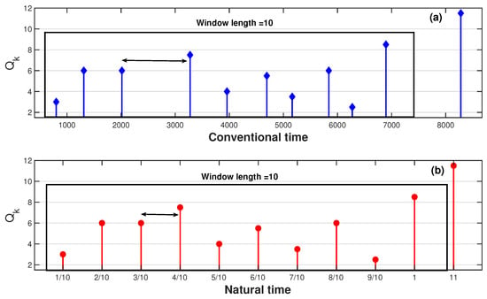
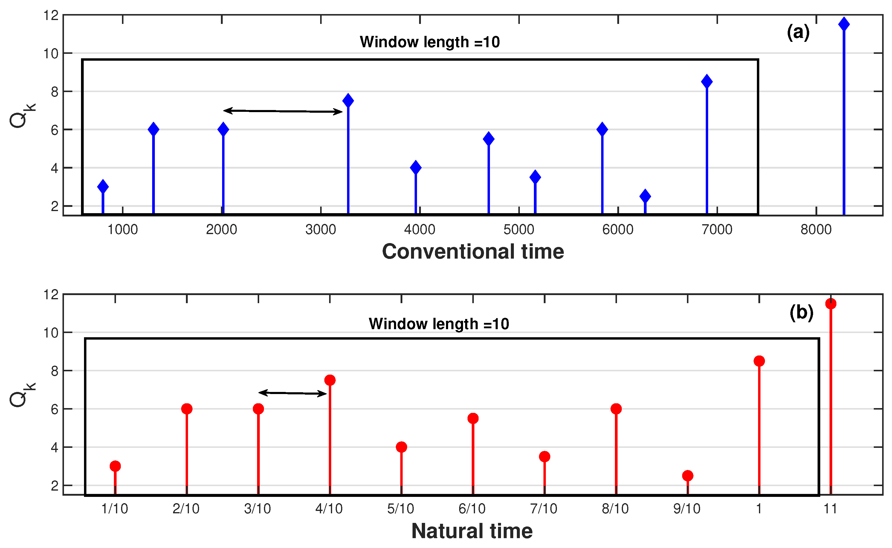
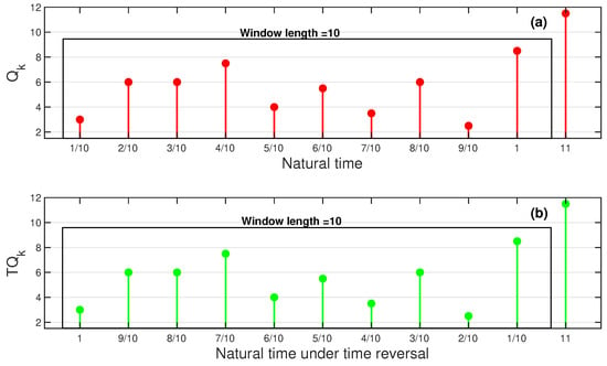
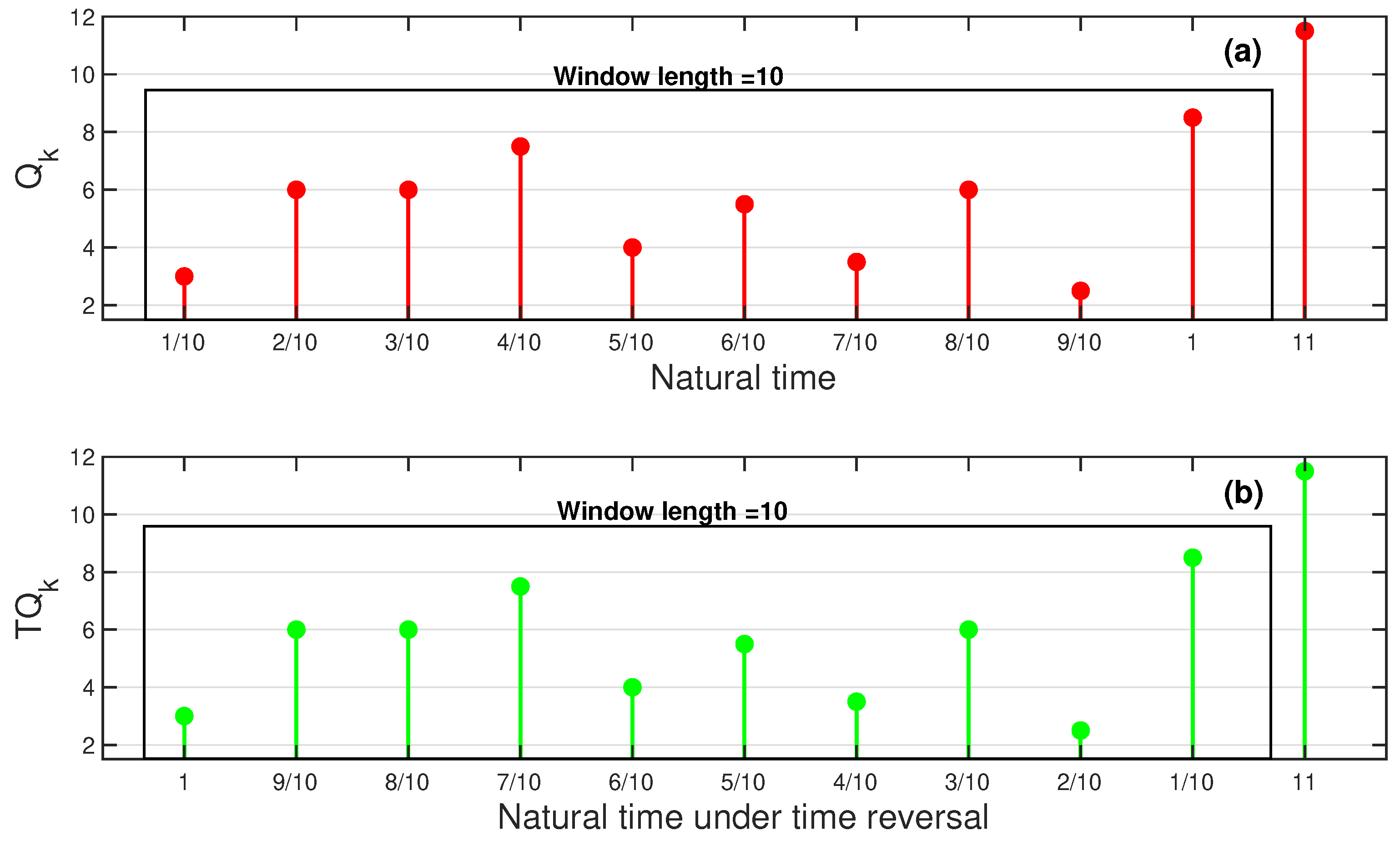
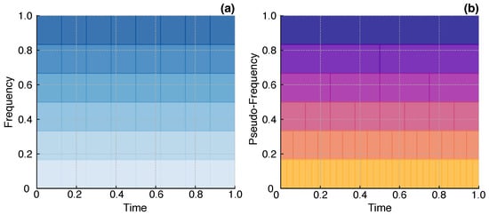
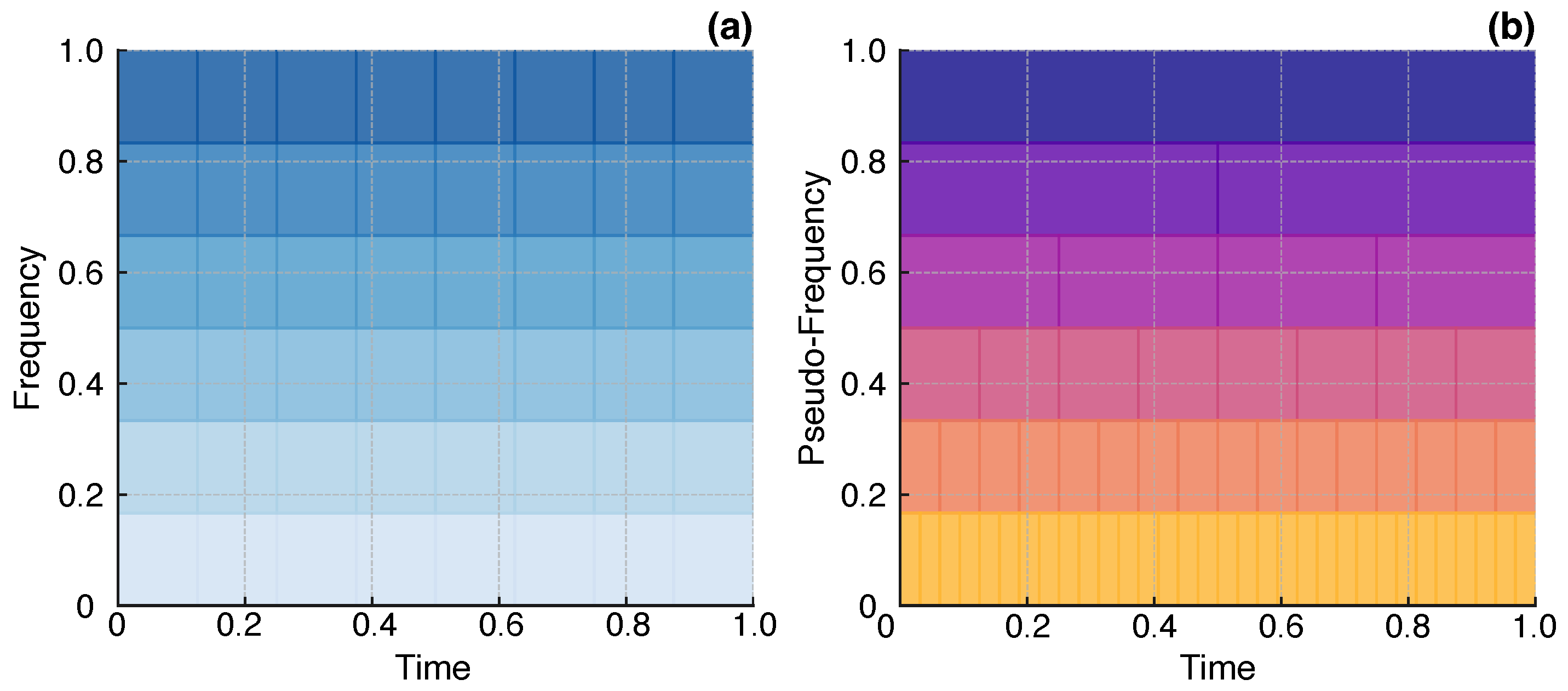
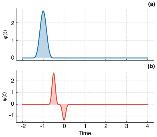
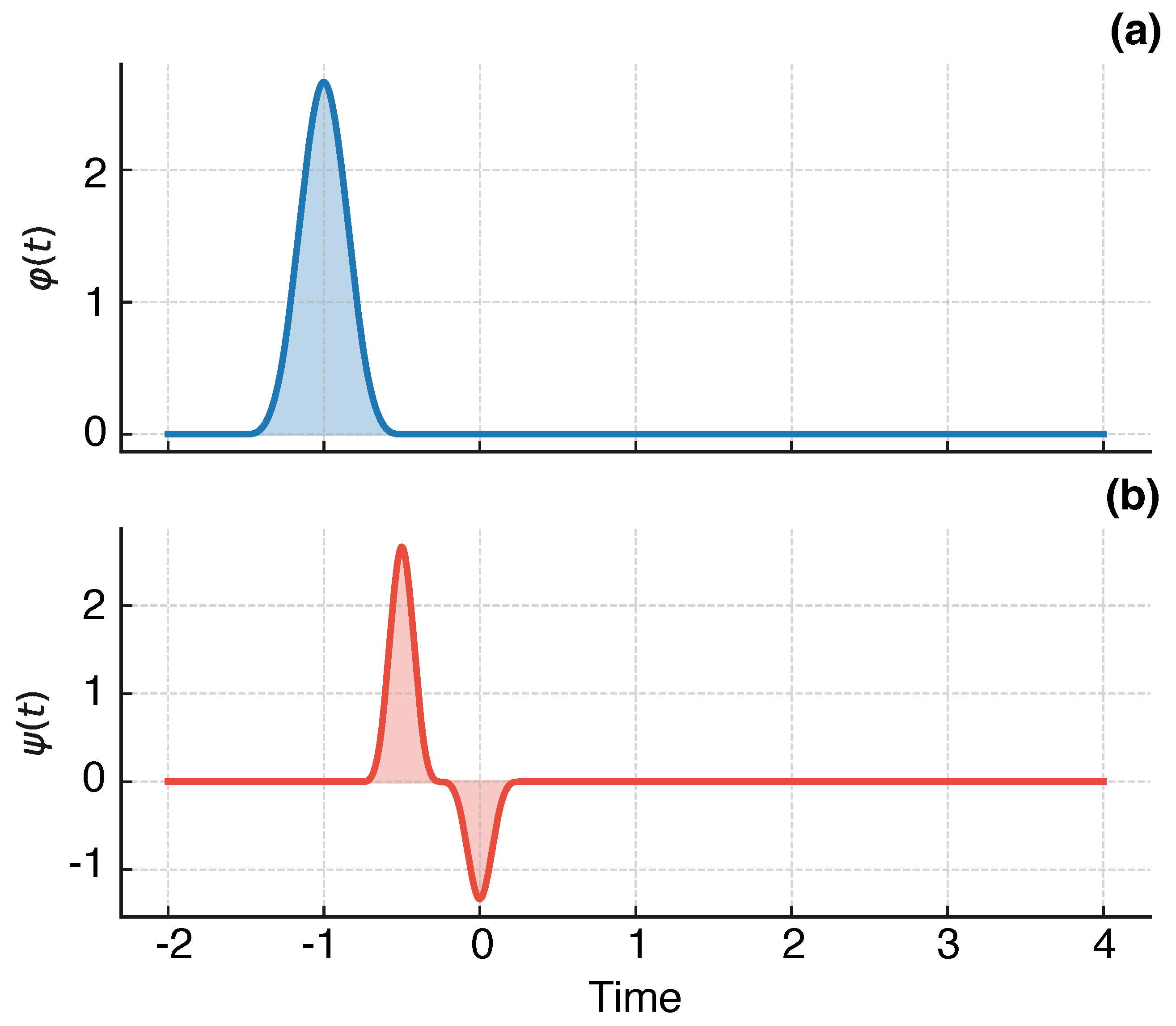
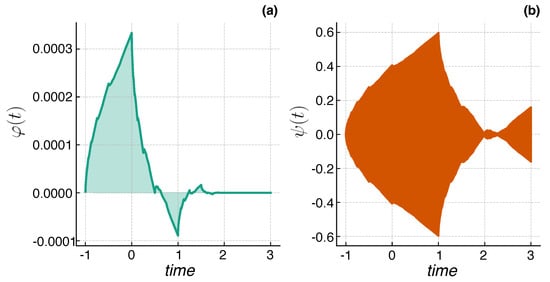
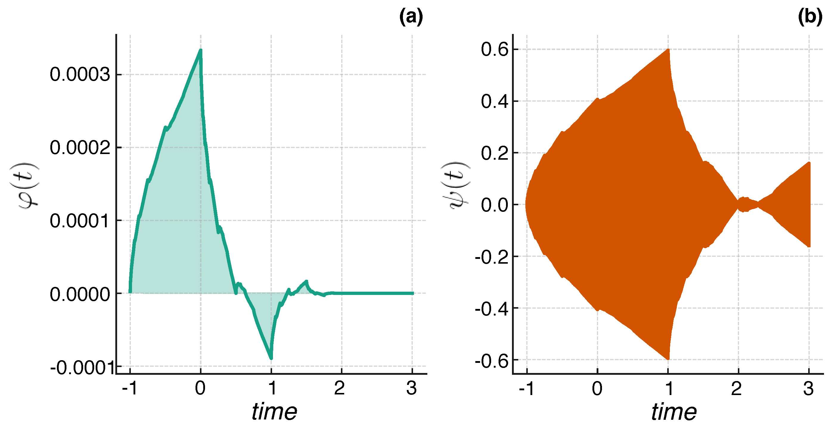
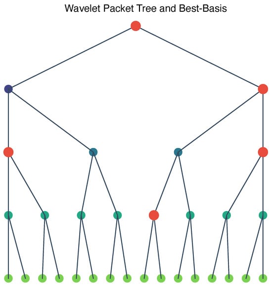
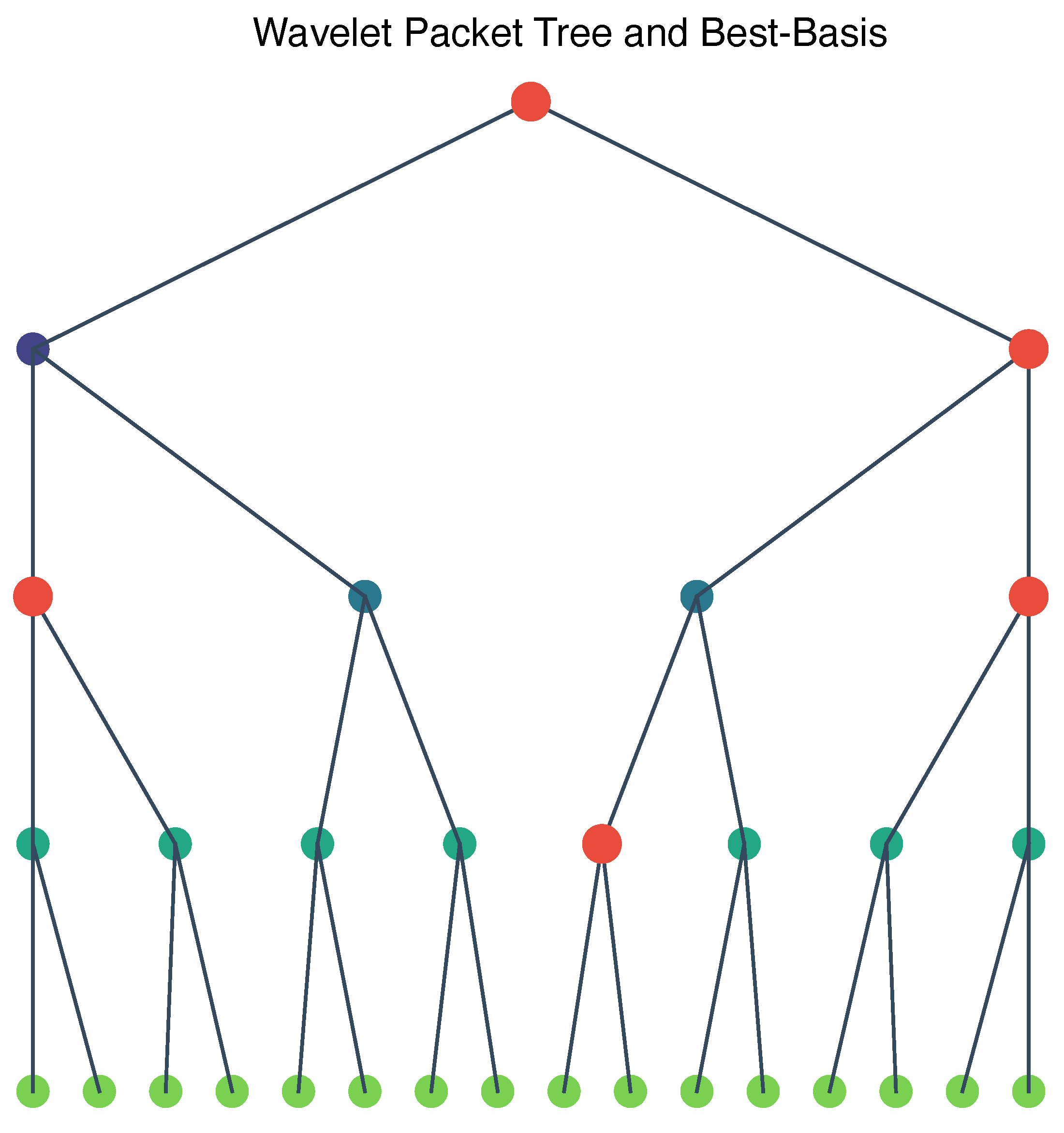
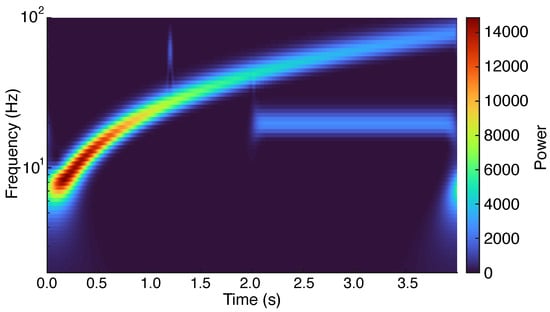
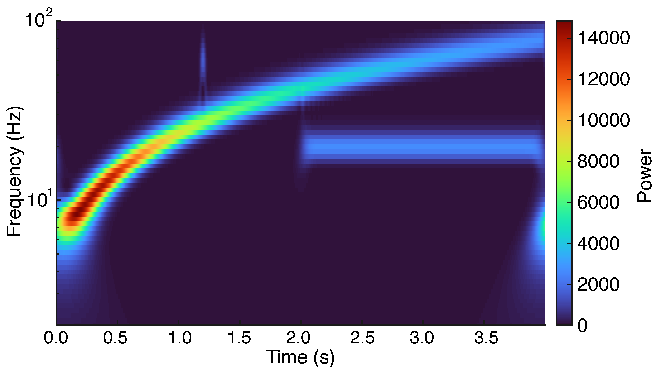
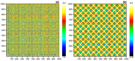
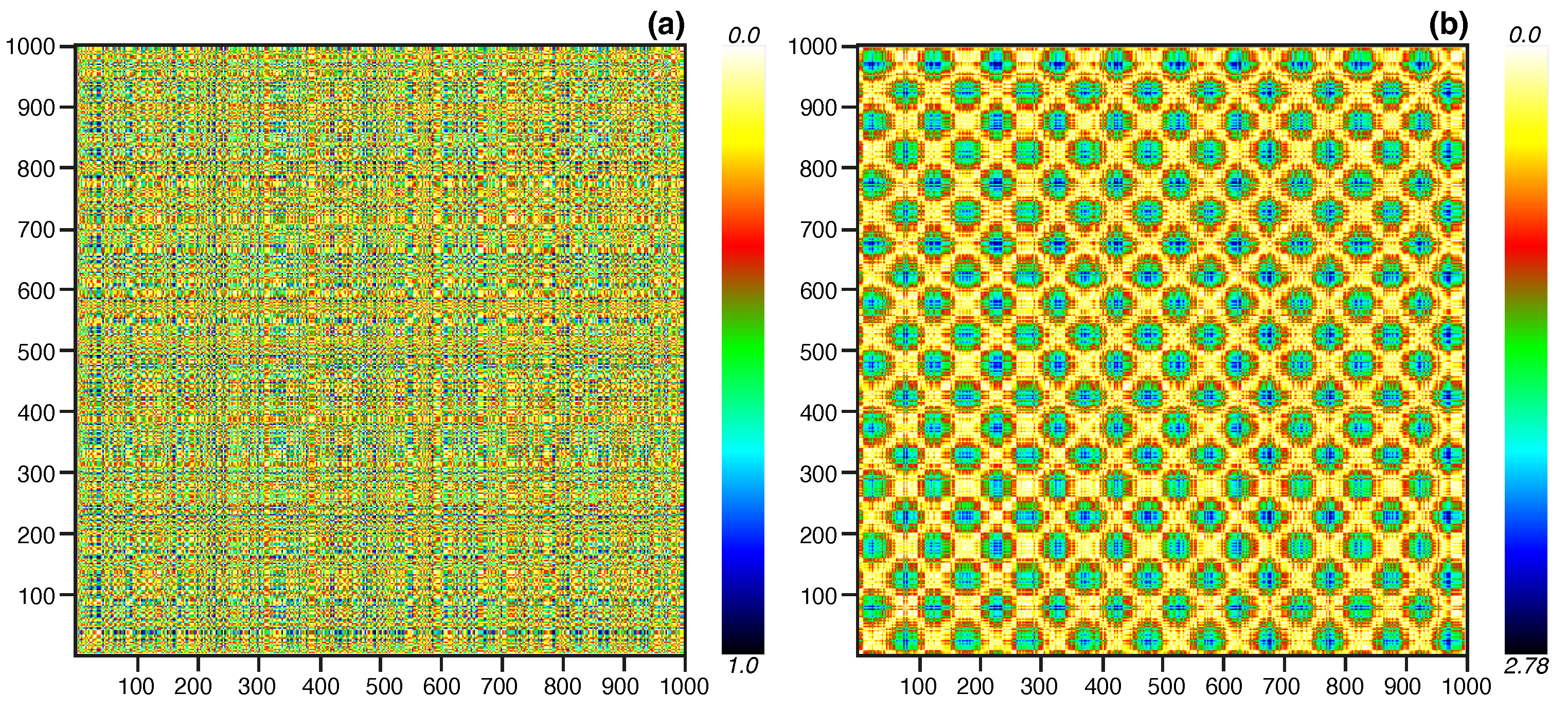
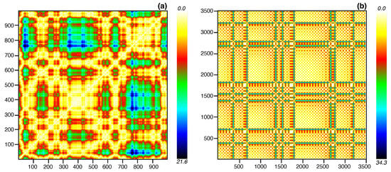
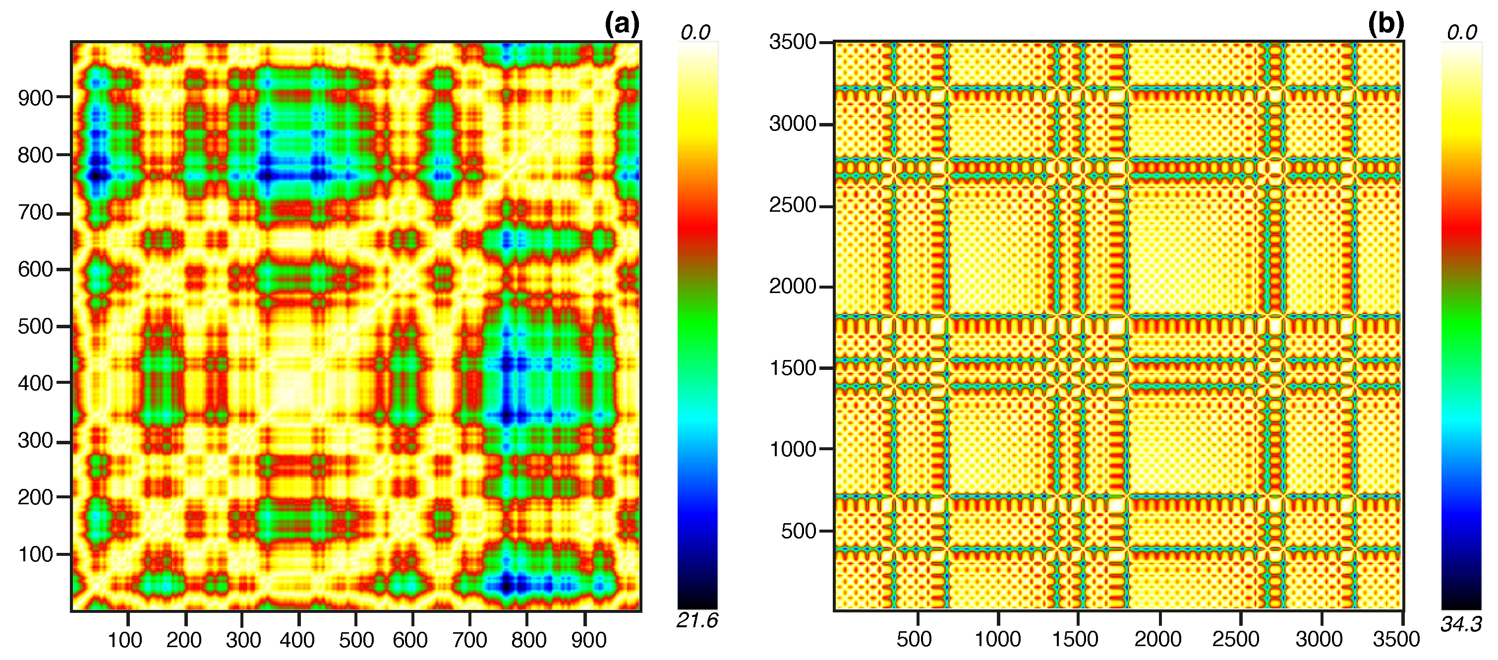
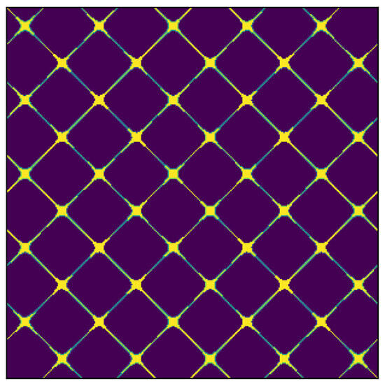
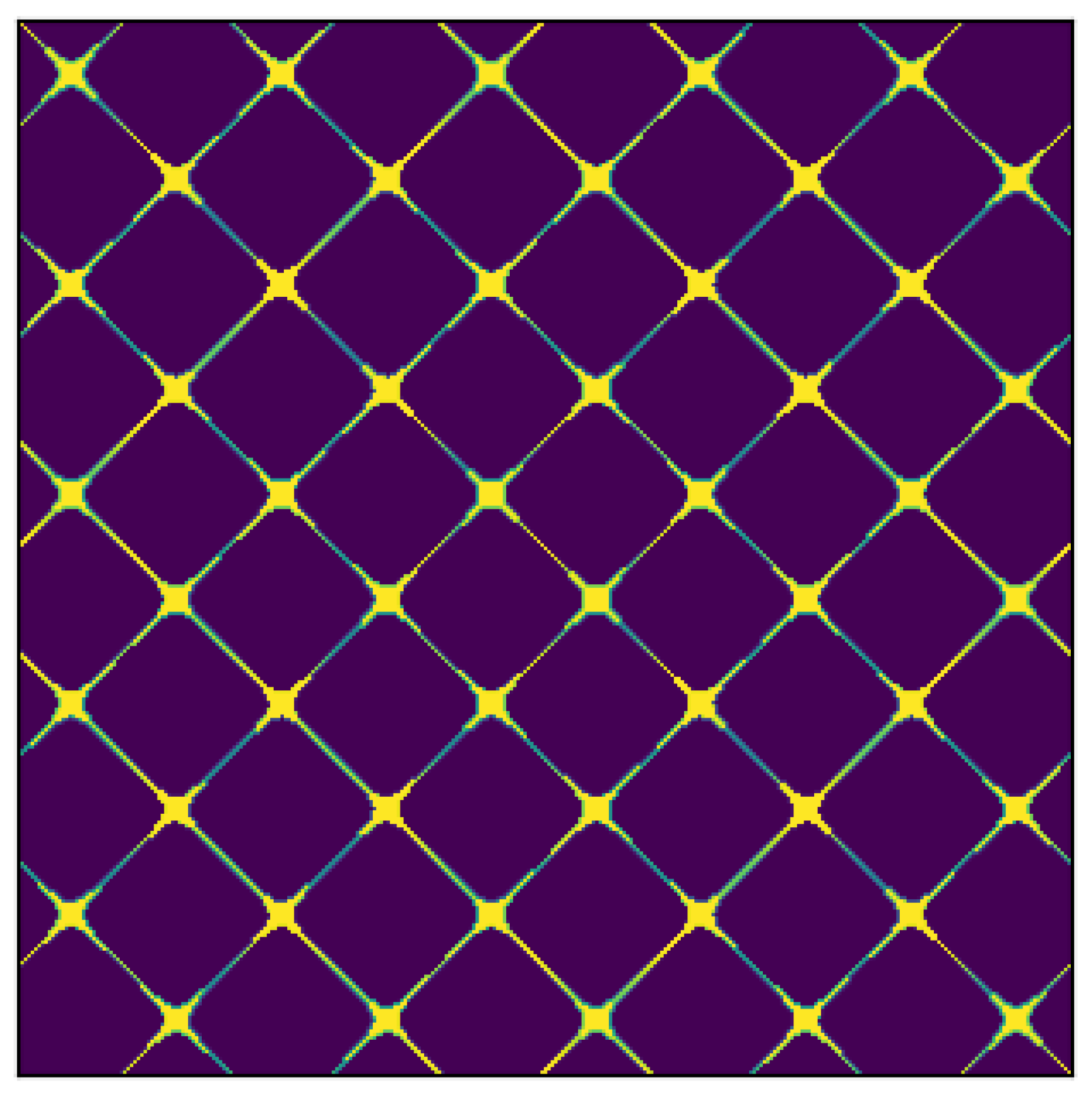
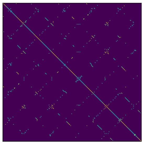
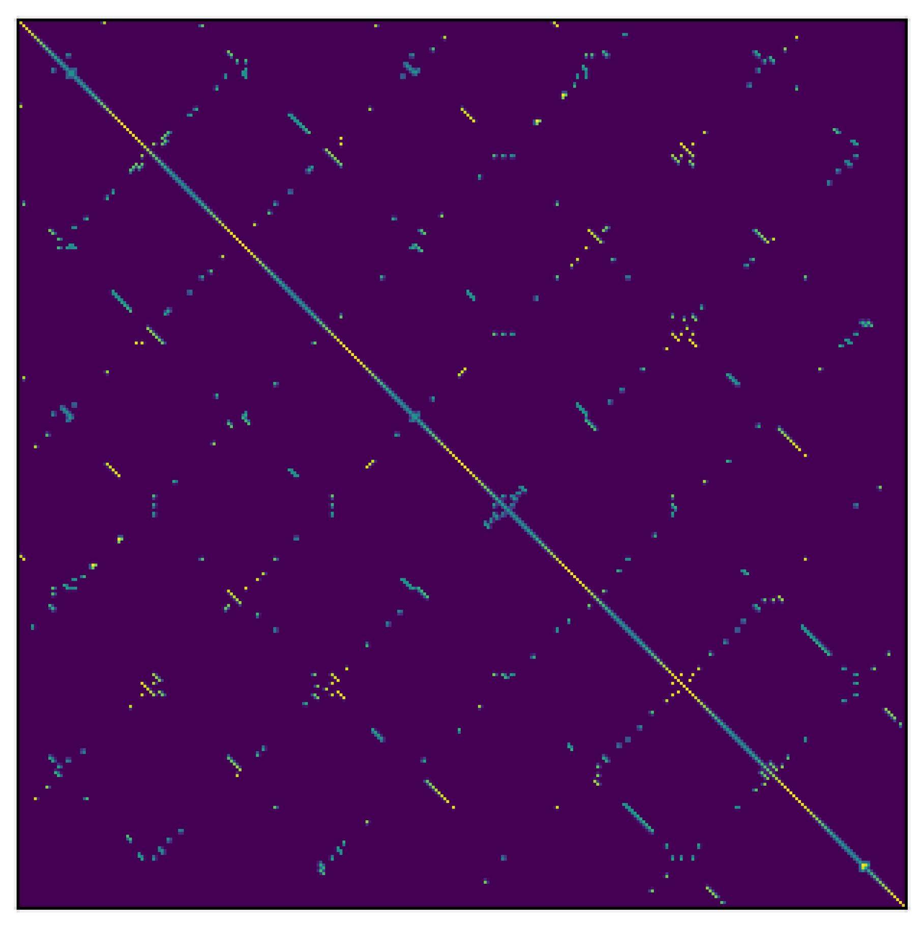

Disclaimer/Publisher’s Note: The statements, opinions and data contained in all publications are solely those of the individual author(s) and contributor(s) and not of MDPI and/or the editor(s). MDPI and/or the editor(s) disclaim responsibility for any injury to people or property resulting from any ideas, methods, instructions or products referred to in the content. |
© 2026 by the authors. Licensee MDPI, Basel, Switzerland. This article is an open access article distributed under the terms and conditions of the Creative Commons Attribution (CC BY) license.