A Stable Rolling Forecast for Renewable Energy Generation Based on a Neural Ordinary Differential Equation

Abstract

Accurate and long-horizon forecasting is essential for reliable planning of solar and wind power generation. Most existing models rely on high-resolution meteorological data, which are often unavailable in practical microgrid environments. This study proposes SNORF, a solar–wind neural ordinary differential equation model that uses only basic meteorological variables such as solar radiation, cloud cover, and wind speed together with lagged generation values. However, reliance on lagged generation inherently limits the effective forecasting horizon of conventional models. To address this limitation, SNORF extends the forecasting horizon while maintaining accuracy and stability through a rolling forecasting framework with a bounded input-dependent drift function and repeated Euler integration that promotes smooth hidden-state dynamics. SNORF supports both deterministic point forecasting and probabilistic forecasting through quantile-based loss functions. Experiments on solar and wind power datasets show that SNORF consistently outperforms representative time-series forecasting models. For solar forecasting, SNORF reduces RMSE and MAE by 15.35% and 16.93% on average compared with baseline models. For wind forecasting, the improvements reach 44.77% in RMSE and 52.85% in MAE on average. Furthermore, when evaluated under the official protocol of the 2024 IEEE Hybrid Energy Forecasting and Trading Competition, SNORF achieves a top 4% ranking using only the officially provided basic weather dataset, demonstrating its practical applicability to renewable energy forecasting in microgrids and virtual power plants.

1. Introduction

Microgrids coordinate distributed energy resources such as photovoltaic systems and wind turbines [1,2]. Because renewable generation is highly sensitive to weather conditions and seasonal variability [3,4], accurate long-horizon forecasting is essential for reliable microgrid operation [5]. To overcome this challenge, it is essential not only to ensure accurate predictions but also to extend the forecasting horizon [6]. Traditional statistical and machine learning approaches, including artificial neural networks (ANNs), support vector machines (SVMs), and random forests (RFs), have been applied to power generation forecasting but show limited ability to capture temporal dependencies and nonlinear dynamics [7,8].

More recently, deep learning architectures such as long short-term memory (LSTM) networks, gated recurrent units (GRUs), and Transformer models have achieved high short-term accuracy by leveraging high-resolution meteorological data and exogenous variables [9,10]. Related machine learning approaches have also been explored for modeling nonlinear physical systems and renewable energy processes [11,12]. However, such data are often unavailable in microgrid-scale environments, and these models still struggle with long-horizon prediction due to error accumulation and limited temporal generalization [13,14].

Therefore, we aim to move beyond this conventional paradigm by leveraging the intrinsic time-series nature of power generation data. In practice, lagged generation values, which represent previously observed power outputs reflecting the most recent state of the system, provide essential temporal context and are readily available in microgrid environments. Feature importance analysis based on the random forest model (Section 3.4) confirms that these lagged values are the most influential predictors for forecasting future solar and wind generation. Incorporating such historical information enables the model to capture short-term dependencies and recurring diurnal patterns [15,16], thereby improving short-horizon accuracy.

However, reliance on past generation inevitably limits the forecast horizon, since models that use lagged generation values can only predict effectively within the temporal range defined by those lags. To overcome this limitation, we adopt a rolling-forecast framework [17], in which the model’s prior predictions are recursively used as inputs for subsequent steps [18]. This recursive strategy enables continuous long-horizon forecasting by combining lagged generation values, which are most correlated with future outputs, and basic meteorological variables (e.g., solar radiation, cloud cover, wind speed, and wind direction), without relying on additional high-resolution numerical weather prediction (NWP) data or mesoscale ensemble prediction systems (MEPS). Through this approach, the model can extend forecasting beyond the observed window while maintaining consistency under data-constrained conditions.

A major drawback of this framework, however, is error accumulation: small prediction errors at each step can compound over time, leading to diverging outputs that become unstable or oscillatory [19,20]. Such instability not only degrades forecasting accuracy but also impairs operational decisions related to power dispatch and energy trading in microgrids, where sudden fluctuations in solar irradiance and wind speed are common [21]. Several studies have proposed post hoc smoothing or filtering techniques to mitigate this issue [16,22,23], but these methods only adjust the outputs rather than addressing the architectural source of instability. A key research question therefore arises: How can we design a forecasting model that intrinsically maintains temporal stability within a rolling forecast framework to achieve accurate long-term forecasting without relying on high-resolution meteorological data?

To address this challenge, we propose SNORF, a solar–wind neural ordinary differential equation (ODE) architecture designed to stabilize recursive time-series forecasting. While rolling forecasting enables long-horizon prediction, it inherently introduces error accumulation due to recursive feedback. SNORF addresses this challenge through architectural mechanisms that constrain hidden-state dynamics during recursive prediction. Unlike conventional neural ODE models that primarily focus on continuous-time representation learning and often rely on adaptive high-order solvers, SNORF introduces two structural modifications tailored for forecasting stability: an input-dependent bounded drift function and repeated Euler integration. These mechanisms constrain hidden-state transitions and induce smooth, low-pass-filter-like state evolution, which mitigates error amplification and suppresses oscillatory predictions under sparse and volatile conditions.

We evaluate SNORF against representative time-series forecasting models using a rolling prediction framework, focusing on both prediction accuracy and temporal stability. Despite relying only on the officially provided dataset, without additional meteorological inputs or external data sources, SNORF ranks within the top 4% on the 2024 IEEE Hybrid Energy Forecasting and Trading competition (HEFTcom24) benchmark, demonstrating its robustness and practical utility for renewable energy forecasting in microgrids and virtual power plants.

The key contributions of this study are summarized as follows:

• This study presents SNORF, a neural ODE-inspired forecasting architecture designed to stabilize recursive time-series prediction.
• An input-dependent bounded drift function that constrains hidden-state dynamics and mitigates instability during recursive forecasting.
• A repeated fixed-step Euler integration scheme that induces smooth hidden-state evolution and suppresses oscillatory predictions.
• Empirical evidence demonstrating that the proposed architectural mechanisms significantly reduce error accumulation in rolling forecasting scenarios.

The remainder of this paper is organized as follows: Section 2 outlines the problem formulation; Section 3 describes the methodology; Section 4 details the experimental setup; Section 5 presents the results; Section 6 discusses the findings; and Section 7 concludes with key insights and future directions.

2. Problem Formulation

We formulate the problem of renewable power generation forecasting within a rolling forecast framework. At each forecasting instant t, the objective is to predict the future generation value $y_{t+h}\in \mathbb{R}$ for horizons $h=1,\dots ,H$, using only information available up to time t. Formally, the information set available at time t is defined as

$${\mathcal{I}}_t=\{(y_{t-i},x_{t-i})\mid i=0,1,\dots ,w-1\},$$

(1)

where $y_{t-i}$ denotes historical generation observations and $x_{t-i}\in {\mathbb{R}}^d$ represents commonly available meteorological variables such as solar irradiance, temperature, wind speed, and cloud cover, which are used as basic input features for forecasting solar and wind power generation, as summarized in Appendix B. Accordingly, the input matrix $X_t\in {\mathbb{R}}^{w\times d}$ thus contains all feature vectors within the look-back window of length w. The goal of the forecasting model $f_{\theta }(\times )$ parameterized by $\theta$ is to generate an estimate ${\widehat{y}}_{t+h}$ conditioned on the observed information set ${\mathcal{I}}_t$:

$${\widehat{y}}_{t+h}=f_{\theta }\left({\mathcal{I}}_t\right),h=1,\dots ,H.$$

(2)

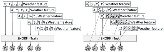
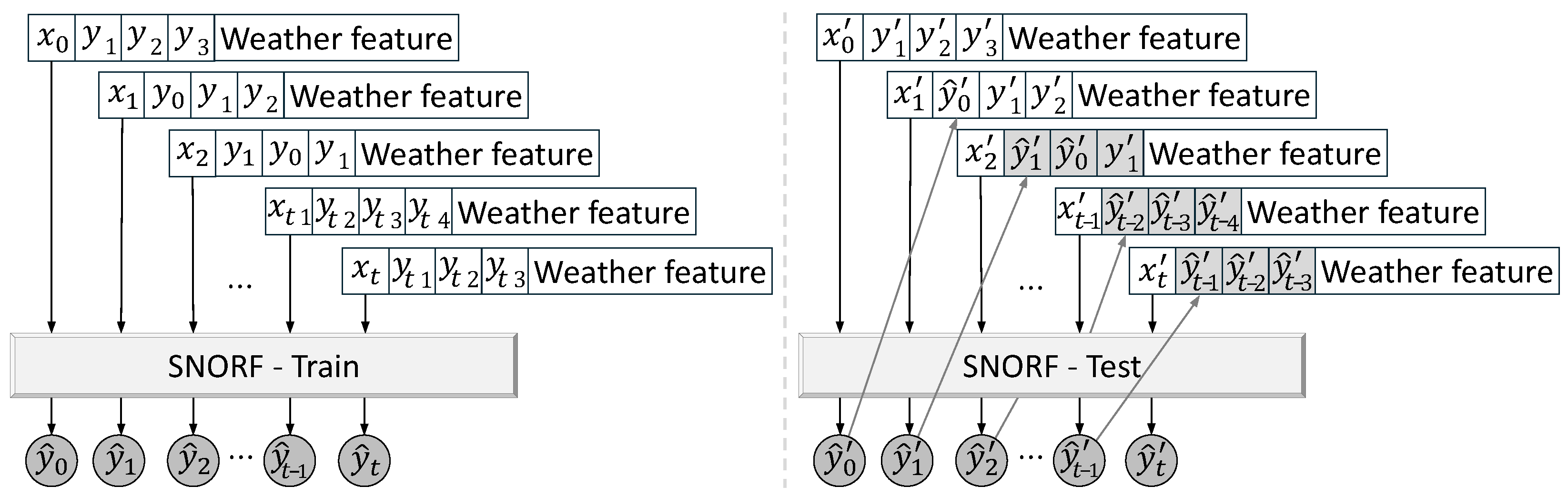
To address the absence of ground-truth values beyond the current time during inference, we employ a rolling forecast strategy, as illustrated in Figure 1. In this framework, the model recursively uses its own prior predictions as inputs to forecast subsequent steps. The recursive prediction at each horizon h is defined as:

$${\widehat{y}}_{t+h}=f_{\theta }({\widehat{y}}_{t+h-1},{\widehat{y}}_{t+h-2},\dots ,{\widehat{y}}_{t+h-k},x_{t+h}),h=1,\dots ,H,$$

(3)

where k denotes the number of lagged output terms used, and $x_{t+h}$ represents the available exogenous features at time $t+h$. If future exogenous features are unavailable (as in many practical microgrid settings), the model relies solely on its own past predictions.

Figure 1. Rolling forecast framework defined in this paper.

While rolling forecasts are widely used for online, data-constrained prediction, they are inherently prone to error accumulation. Let $e_t={\widehat{y}}_t-y_t$ denote the prediction error at time t. Assuming that the forecasting function f is Lipschitz continuous with respect to its inputs, the error propagation across steps can be approximately bounded as:

$$|e_{t+1}|\le L\times |e_t|,$$

(4)

where L is the Lipschitz constant of the model. Many neural network architectures satisfy this assumption under common activation functions such as ReLU or tanh, whose derivatives are bounded. For feedforward neural networks, the overall Lipschitz constant is determined by the product of the spectral norms of the weight matrices across layers, making the Lipschitz assumption reasonable for analyzing error propagation in recursive prediction.

Equation (4) provides an intuitive interpretation of error amplification in rolling forecasting. If the model slightly overestimates the generation at one time step, that prediction becomes part of the input for the next step. Consequently, the error may propagate and accumulate across recursive predictions. When $L>1$, the magnitude of the error can increase multiplicatively at each step, leading to exponential error growth and potentially unstable or oscillatory forecasts. In contrast, if $L<1$, the recursive prediction process becomes contractive, and the forecasting error gradually decays over time.

In practice, however, strictly constraining $L<1$ in nonlinear forecasting models is often infeasible, as it may reduce expressive capacity and optimization flexibility [24].

From this perspective, the forecasting model is trained by minimizing the prediction loss over the forecasting horizon:

$$\underset{\theta }{min}{\mathcal{L}}_{\mathrm{forecast}}({\widehat{y}}_{t:t+H},y_{t:t+H}),$$

(5)

where ${\mathcal{L}}_{\mathrm{forecast}}$ denotes the prediction loss (e.g., mean squared error).

Instead of explicitly enforcing a hard Lipschitz constraint during training, we use the Lipschitz condition as a theoretical perspective for understanding error amplification in recursive forecasting. The model architecture is designed to implicitly encourage bounded hidden-state dynamics. In particular, SNORF employs a bounded nonlinear drift function and repeated small-step Euler updates, which help limit abrupt hidden-state transitions and mitigate error amplification under recursive rolling prediction. This architectural design provides a practical mechanism for improving long-horizon forecasting robustness.

3. Methodology

This section outlines the structure of SNORF, as well as the dataset, preprocessing and postprocessing steps, and feature engineering techniques.

3.1. Structure of SNORF

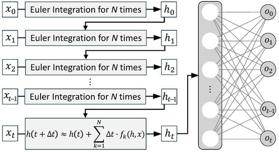
SNORF is a modified neural ODE model specifically designed for time-series forecasting. Its architecture, illustrated in Figure 2, introduces several innovations aimed at improving stability in recursive prediction tasks.

Figure 2. Structure of the proposed SNORF model.

The model features four key architectural components:

• Input-dependent, non-autonomous drift function: Dynamically adapts to varying inputs, capturing time-varying dynamics.
• Euler-based solver: Provides numerically simple and stable integration without relying on high-order ODE solvers.
• Flexible input configuration: Supports both sequential and pointwise inputs for rolling forecasts.
• Embedded structural inductive bias: Encourages smooth transitions and helps suppress oscillations in predictions.

In classical neural ODE formulations, higher-order solvers such as Runge–Kutta methods are commonly used to accurately approximate continuous-time dynamics. However, in recursive forecasting settings, solver accuracy is often less critical than numerical stability and computational efficiency. Higher-order solvers introduce additional function evaluations per step, which can significantly increase computational cost without necessarily improving predictive stability in long-horizon recursive prediction. In contrast, the fixed-step Euler integration used in SNORF provides a simple and stable update rule. When combined with bounded nonlinear activations, the Euler update behaves similarly to a low-pass filter on hidden-state dynamics, suppressing high-frequency oscillations that can otherwise amplify during recursive forecasting. This property makes Euler integration particularly suitable for stabilizing long-horizon predictions.

By addressing the practical requirements of adaptability and forecast stability, SNORF extends conventional neural ODEs for more effective use in recursive time-series forecasting. From a computational perspective, SNORF has complexity comparable to recurrent models such as LSTM. Each Euler update involves matrix multiplications between hidden states and weight matrices, resulting in approximately $O\left(TU{H}^2\right)$ complexity for a sequence of length T with U unfolding steps and hidden dimension H. Unlike Transformer models, which require $O\left(T^{2}H\right)$ operations due to self-attention, SNORF scales linearly with the sequence length and avoids the quadratic complexity introduced by self-attention mechanisms in Transformer models, making it well suited for real-time prediction and practical deployment in microgrid environments.

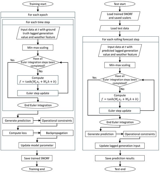
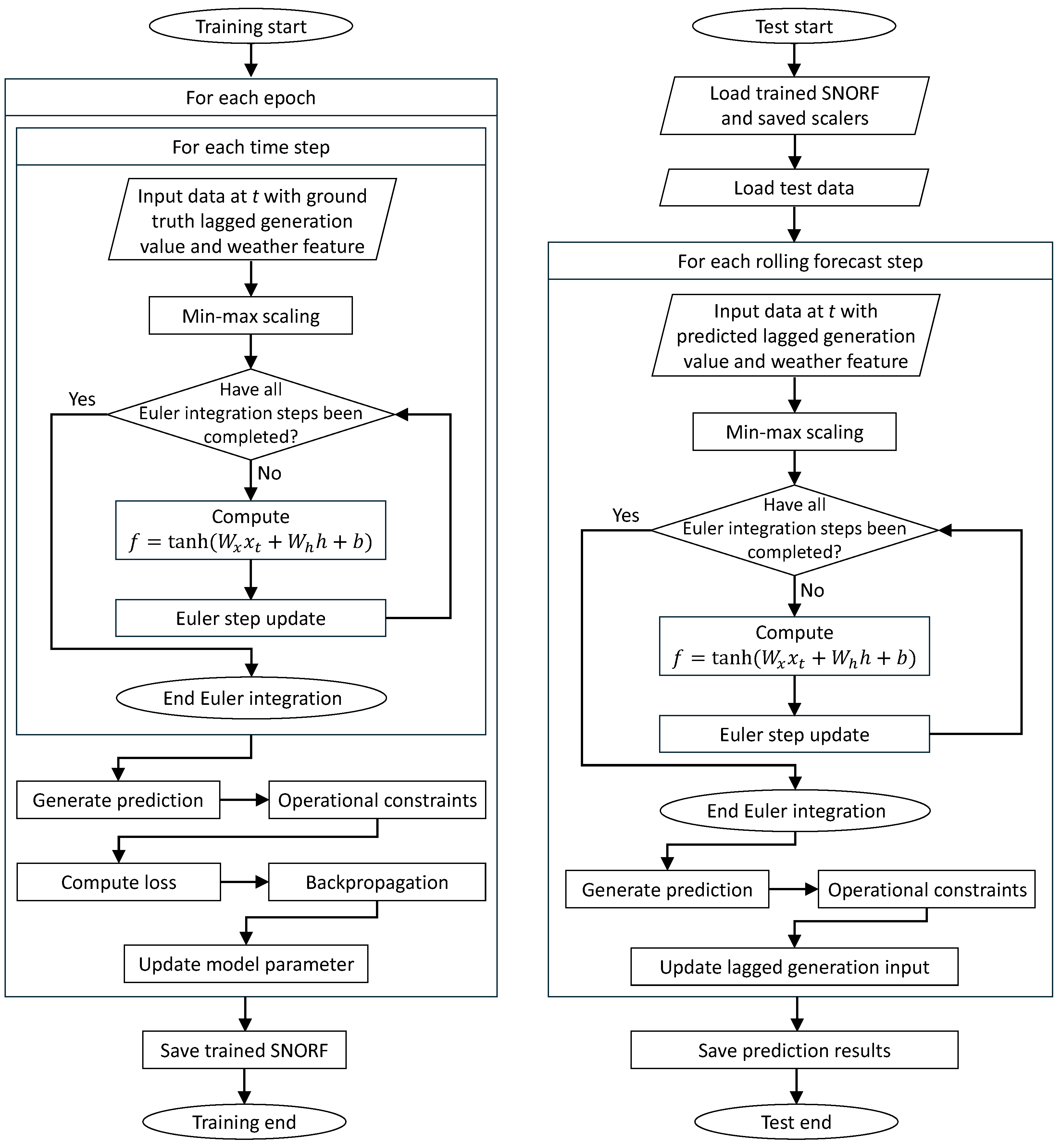
While the architectural design of SNORF focuses on the model structure, it is also necessary to clarify the overall training and inference procedure. To provide a clearer understanding of the overall procedure of the proposed method, Figure 3 illustrates the complete training and testing workflow of SNORF. The flowchart summarizes the recursive rolling forecasting mechanism, in which previously predicted values are fed back as lagged inputs, as well as the Euler-based hidden-state update governed by a bounded drift function. During training, the model parameters are optimized through loss computation and backpropagation, while during testing, the trained model generates predictions in an autoregressive manner with operational constraints applied to ensure physically feasible outputs.

Figure 3. Flowchart of the training and testing procedures of SNORF.

The overall computational procedure described above is formally summarized in Algorithm 1. In addition to architectural flexibility, SNORF supports both deterministic point forecasting and probabilistic forecasting depending on the requirements of the application. For point forecasting tasks, the model produces a single prediction and can be trained using a standard regression loss. For probabilistic forecasting, the model predicts multiple quantiles using quantile-specific output heads. In recursive rolling prediction, the median forecast is used as the feedback input for the next step. This design allows SNORF to flexibly adapt to different operational scenarios and user requirements, supporting both deterministic prediction tasks and uncertainty-aware forecasting applications.

Algorithm 1 Main algorithm of SNORF
Inputs: Feature sequence $X\in {\mathbb{R}}^{T\times d}$, number of ODE unfolding steps U
Outputs: Predicted target value $\widehat{y}\in \mathbb{R}$ (point forecast) or predicted quantile vector $\widehat{\mathbf{q}}\in {\mathbb{R}}^{N_q}$ (probabilistic forecast)
Definitions: Number of time steps T, feature dimension d, number of quantiles $N_q$
Initialize hidden state $h\leftarrow 0$
Set time resolution step $\Delta t\leftarrow 1/U$
for each time step $t=1$ to T do
$x_t\leftarrow X\left[t\right]$	// Extract input at time t
for $u=1$ to U do
$f\leftarrow tanh(W_x{x}_t+W_{h}h+b)$	// Drift function
$h\leftarrow h+\Delta t\times f$	// Euler step update
end for
end for
$z\leftarrow ReLU\left({Linear}_1\left(h\right)\right)$
$z\leftarrow Dropout\left(z\right)$
if point forecasting then
$\widehat{y}\leftarrow Linear\left(z\right)$
return $\widehat{y}$
else
Initialize $Q\leftarrow \left[\right]$
for $i=1$ to $N_q$ do
${\widehat{q}}_i\leftarrow {LinearQuantile}_i\left(z\right)$
Append ${\widehat{q}}_i$ to Q
end for
$\widehat{\mathbf{q}}\leftarrow Concatenate\left(Q\right)$
return $\widehat{\mathbf{q}}$
end if

To fully leverage this input flexibility while maintaining model efficiency, we employed hyperparameter optimization using the Optuna framework [25]. The search space included learning rate, batch size, hidden size, dropout rate, the $\rho$ value of the sharpness-aware minimization (SAM) optimizer [26], input sequence length, and the number of ODE unfolding steps. After the hyperparameter search, the final models were trained for up to 500 epochs with early stopping based on validation loss (patience = 10). The resulting optimized hyperparameters used for solar and wind forecasting are summarized in Table 1 and Table 2, respectively.

Table 1. Optimal hyperparameters of SNORF solar model.

Parameter	Value	Range	Method
Input type	Sequence	[Sequence, Pointwise]	Categorical
Timestep	3	[1, 10]	Discrete (step = 1)
Hidden size	20	[16, 64]	Uniform
Linear hidden size	401	[128, 512]	Uniform
ODE unfold	3	[1, 5]	Discrete (step = 1)
SAM $\rho$	0.0284	[0.01, 0.1]	Uniform
Dropout	0.1124	[0.0, 0.3]	Uniform
Learning rate	0.0030	[${10}^{-4}$, ${10}^{-2}$]	Log-uniform
Batch size	256	[64, 128, 256]	Categorical

Table 2. Optimal hyperparameters of SNORF wind model.

Parameter	Value	Range	Method
Input type	Pointwise	[Sequence, Pointwise]	Categorical
Hidden size	17	[16, 64]	Uniform
Linear hidden size	287	[128, 512]	Uniform
ODE unfold	8	[1, 10]	Discrete (step = 1)
SAM $\rho$	0.0105	[0.01, 0.1]	Uniform
Dropout	0.1333	[0.0, 0.3]	Uniform
Learning rate	0.0004	[${10}^{-4}$, ${10}^{-2}$]	Log-uniform
Batch size	128	[64, 128, 256]	Categorical

3.2. Dataset

The HEFTcom24, organized by the IEEE Power & Energy Society and sponsored by Ørsted (Fredericia, Denmark) and rebase.energy (Stockholm, Sweden), serves as a benchmark for state-of-the-art forecasting methods [27]. Held in real-time from February to May 2024, the competition focused on probabilistic forecasting of aggregated power output from the Hornsea 1 offshore wind farm and solar power facilities in eastern England, using quantile regression evaluated via Pinball Score. Participants were also tasked with formulating energy trading strategies based on these forecasts. We utilize the official HEFTcom24 dataset, which includes numerical weather forecasts from the Deutscher Wetterdienst (DWD) ICON-EU (Icosahedral Nonhydrostatic–European) model and corresponding power generation records.

In this study, only the basic meteorological variables provided by the DWD forecasts together with the corresponding generation data were used for model training and evaluation. Table 3 summarizes the basic statistics of the meteorological and generation variables used in this study, including their mean values, standard deviations, and missing data rates. The training set spans from 20 September 2020 to 19 February 2024, and was used to develop and optimize the model. The test set, covering 20 February to 19 May 2024, was held out for final evaluation. Additional details regarding the dataset and input features are provided in Appendix B.

Table 3. Basic statistics of the dataset variables.

Feature	Mean	Std.	Missing Rate (%)
Wind speed at 10 m (WindSpeed)	7.56	15.06	0.01
Wind speed at 100 m (WindSpeed_100)	9.43	23.05	0.01
Wind power generation (Wind_MW)	573.89	192,201.14	0.18
Solar radiation (Radiation)	100.02	23,755.89	0.01
Solar plant temperature (Temperature)	10.70	36.63	0.01
Cloud cover (CloudCover)	0.72	0.08	0.01
Solar power generation (Solar_MW)	229.62	142,139.99	0.12

3.3. Pre-Processing and Post-Processing

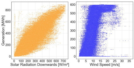
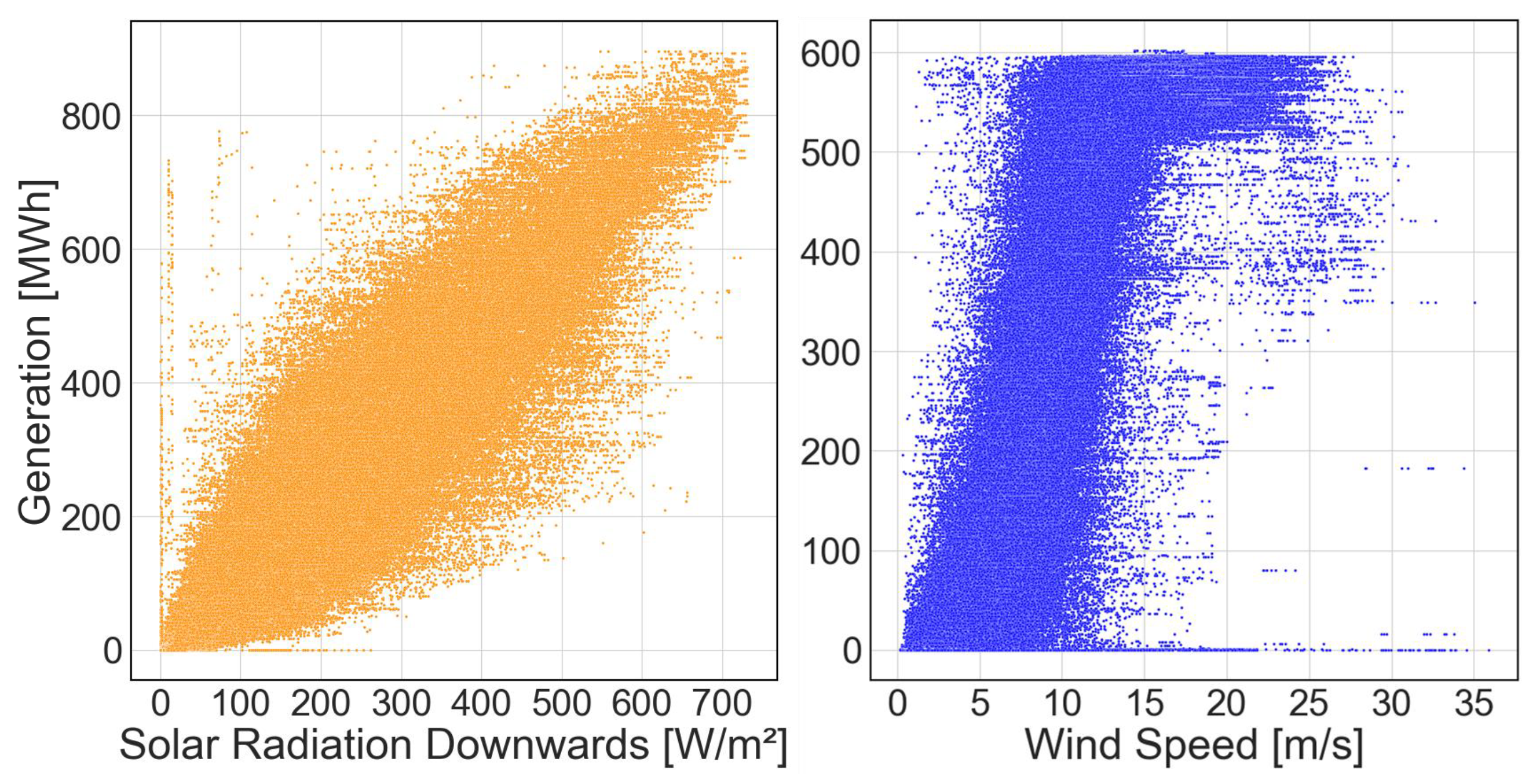
Figure 4 shows the irregular and non-stationary patterns of solar and wind power output, which generally correlate with solar irradiance and wind speed, respectively. These irregularities may result from curtailment, control constraints, or sudden changes in weather conditions. Although imputation techniques are commonly applied to handle missing values and outliers, they can distort the underlying data distribution or introduce unnecessary computational overhead. Moreover, artificially filling missing values can obscure potentially informative patterns inherent in the missingness itself.

Figure 4. Scatter plots of solar and wind power generation.

Before model training, continuous input variables were normalized using Min–Max scaling to improve numerical stability and training convergence. Specifically, each feature x was transformed as

$$x^{\prime }={\displaystyle \frac{x-x_{min}}{x_{max}-x_{min}}},$$

(6)

where $x_{min}$ and $x_{max}$ denote the minimum and maximum values estimated from the training data. The same scaling parameters were subsequently applied to the validation and test sets to avoid data leakage. The target variable was also scaled using the same Min–Max transformation during training and later rescaled to the original physical units for evaluation.

To preserve data integrity and allow the model to learn from natural variability, we chose not to apply any artificial imputation. In the post-processing stage, source-specific physical constraints were enforced. For solar power, predictions outside the feasible daylight window were set to zero. For wind power, predictions were capped at the installed capacity. In both cases, negative outputs were clipped to zero to reflect physical constraints.

3.4. Feature Engineering

To improve forecasting accuracy, we engineered features from the competition-provided meteorological dataset. Temporal features such as month and hour were encoded using trigonometric functions to better capture their inherent cyclicality [28]. Additionally, to represent time-series characteristics more effectively, we generated lag and difference features for each weather variable, including 30 min and 1 h lags, same-time values from the previous day, and daily averages. Prior research has shown that incorporating selected past values can significantly enhance both forecast stability and reliability [29].

To quantify the contribution of each feature, we performed a feature importance analysis using a Random Forest model, chosen for its robustness and interpretability [30]. Table 4 presents the top five features ranked by importance for both solar and wind power forecasting. As shown in Table 4, the most influential feature for both solar and wind forecasting was the power generation value from 30 min prior (Solar_MW_30m and Wind_MW_30m, respectively), highlighting the strong predictive value of recent historical data. The consistent importance of lagged features across domains suggests that temporal dependencies are more critical than complex additional variables in rolling forecasts. The selection of 30 min and 1 h lags was guided by domain knowledge, which reflects typical timescales of variation in solar irradiance and wind speed, and this choice was empirically supported by the feature importance analysis.

Table 4. Feature importance ranking for solar and wind power forecasting.

Solar			Wind
Rank	Feature	Importance	Feature	Importance
1	Solar_MW_30m	0.9588	Wind_MW_30m	0.9817
2	Radiation_diff	0.0156	Wind_MW_60m	0.0043
3	Radiation	0.0134	WindSpeed_100_diff	0.0021
4	Temperature_diff	0.0022	Wind_MW_90m	0.0012
5	time_sin	0.0017	WindSpeed_diff	0.0009

These findings confirm that lag features are not merely a workaround for missing data, but essential structural components of effective forecasting models. Moreover, eliminating redundant variables and focusing on informative features reduces model complexity and enhances forecasting stability. This underscores the effectiveness of the feature selection strategy employed in this study, particularly for sequential forecasting under data constraints.

4. Experimental Setup

This section describes the baseline models and the HEFTcom24 benchmark used to validate the proposed SNORF model.

4.1. Baseline Models and Evaluation Metrics

We compared SNORF with representative time-series forecasting models, which are listed in Table 5. For a fair comparison, all models were trained under identical experimental conditions. All models were evaluated using the same rolling forecast framework, where multi-step predictions were generated recursively by feeding each predicted output back as input for the subsequent forecasting step. Hyperparameters for all baseline models were tuned using a unified search strategy, and the final configurations are detailed in Appendix C. All deep learning models were trained on a system equipped with an NVIDIA GeForce RTX 3090 Ti GPU, Intel Core i9-12900K CPU, and Python 3.8, using PyCharm 2025.3.4 development environment.

Table 5. Benchmark time-series models and rationale.

Category	Model	Rationale for Selection
Basic Recurrent Model	RNN (Recurrent Neural Network)	The simplest neural architecture for processing time-series data; used as a baseline to evaluate the performance gap with the proposed model.
Extended Recurrent Model	LSTM	An extension of RNNs with strengths in handling long-term dependencies; a representative benchmark model for rolling forecasting.
Hybrid Model	CNN (Convolutional Neural Network)-LSTM	A hybrid architecture combining CNN’s local feature extraction capabilities with LSTM’s sequence learning ability.
Attention-based Model	Transformer	An attention-based architecture with strong performance in modeling long-term dependencies.
Conventional Neural ODE Model	Neural ODE	A representative continuous-time modeling framework; used as a baseline to assess the effectiveness of the proposed modified Neural ODE structure.

Since the HEFTcom24 benchmark requires probabilistic forecasting, a different set of hyperparameters was used compared with those adopted for the pointwise forecasting model described in Section 3.1. The resulting configurations are summarized in Table 6. Similar to the procedure used in Section 3.1, the hyperparameters were optimized using the Optuna framework [25] within the same search ranges.

Table 6. Hyperparameter configurations for HEFTcom24.

Model	Input Type	Timestep	ODE Unfolds	Learning Rate	Batch Size	Hidden Size	Linear Hidden Size	Dropout	SAM $\mathit{\rho }$
Solar	Sequence	4	3	0.0012	128	26	156	0.2914	0.0268
Wind	Sequence	10	3	0.0089	64	33	187	0.0408	0.0246

4.2. Overview of the HEFTcom24 Benchmark

The HEFTcom24 competition is an international event that provides a standardized benchmark for evaluating joint forecasting and trading strategies in hybrid renewable energy systems, balancing real-world relevance with academic rigor. The competition aims to identify robust forecasting methods under realistic operational constraints, making it particularly relevant for industrial applications. Participants are required to produce day-ahead quantile forecasts of wind and solar power generation and to develop corresponding market strategies. In total, more than 170 teams registered, with 66 teams actively submitting forecasts [31].

The competition comprises two tracks:

• Track 1: Hybrid Energy Forecasting—focusing on aggregated wind and solar power predictions.
• Track 2: Energy Trading—involving strategy design based on forecast outputs.

This study focuses on Track 1—hybrid energy forecasting. The primary evaluation metric is the Pinball Score, a standard loss function used for quantile regression.

The quantile loss function is defined as:

$${\mathcal{L}}_{\alpha }(y,{\widehat{q}}_{\alpha })=\left\{\begin{array}{cc}\alpha (y-{\widehat{q}}_{\alpha }),\hfill & \mathrm{if}y\ge {\widehat{q}}_{\alpha }\hfill \\ (1-\alpha )({\widehat{q}}_{\alpha }-y),\hfill & \mathrm{if}y<{\widehat{q}}_{\alpha }\hfill \end{array}\right.$$

(7)

where y is the true value and ${\widehat{q}}_{\alpha }$ is the predicted quantile at level $\alpha$.

The final Pinball Score (PS) is computed as:

$$\mathit{PS}={\displaystyle \frac{1}{N}}\sum _{i=1}^N{\mathcal{L}}_{\alpha }(y_i,{\widehat{y}}_i)$$

(8)

where N is the total number of forecast instances, and ${\mathcal{L}}_{\alpha }(y_i,{\widehat{y}}_i)$ is the quantile loss for instance i.

The final score is averaged across nine quantiles (from the 10th to 90th percentiles), in accordance with the official HEFTcom24 protocol. This evaluation framework enables comprehensive assessment by capturing both point accuracy and the distributional reliability of forecasts. The HEFTcom24 benchmark evaluates probabilistic forecasts using the Pinball Score. Accordingly, our implementation directly produces probabilistic forecasts by jointly predicting multiple quantiles within a single model, where each quantile is generated by a quantile-specific output head.

5. Experimental Results

5.1. Performance Comparison of Time-Series Models

To evaluate forecasting performance, we use two categories of metrics: (1) accuracy metrics for pointwise prediction errors; (2) a structural metric for temporal consistency.

Accuracy metrics. Root Mean Square Error (RMSE) and Mean Absolute Error (MAE) quantify the pointwise discrepancy between predicted and actual power generation, reflecting the magnitude of forecasting errors.

As a structural metric, the Pearson Correlation Coefficient (PCC) measures the directional alignment between predicted and actual sequences, capturing the similarity of their temporal patterns. It is defined as:

$$r={\displaystyle \frac{{\sum }_{i=1}^n(x_i-\overline{x})(y_i-\overline{y})}{\sqrt{{\sum }_{i=1}^n{(x_i-\overline{x})}^2}\sqrt{{\sum }_{i=1}^n{(y_i-\overline{y})}^2}}}$$

(9)

where $x_i$ and $y_i$ denote the predicted and actual values at time step i, and $\overline{x}$ and $\overline{y}$ are their respective means. The PCC ranges from $-1$ to 1, with higher values indicating stronger temporal correlation and thus greater structural consistency in the forecasted trajectory.

Table 7 and Table 8 present the forecasting performance of SNORF and the baseline models for solar and wind power generation. To ensure a fair comparison, each experiment was repeated 10 times for every model, and the reported values are presented as the mean and standard error (SE). SNORF achieves the lowest RMSE and MAE in both domains, indicating superior pointwise accuracy. It also records the highest PCC scores, reflecting strong alignment with the temporal patterns of actual generation. In addition, SNORF requires the shortest training time among all models, demonstrating its computational efficiency.

Table 7. Performance comparison of solar power forecasting models. Values are presented as mean ± SE. An asterisk (*) indicates SE values rounded to 0.00 due to their small magnitude.

Model	RMSE (%) ± SE	MAE (kWh) ± SE	PCC ± SE	Training Time (s) ± SE
RNN	6.27 ± 0.11	63.85 ± 1.12	0.96 ± 0.00 *	160.57 ± 18.45
LSTM	7.48 ± 0.55	75.38 ± 5.44	0.95 ± 0.01	242.00 ± 27.32
CNN-LSTM	6.87 ± 0.10	69.97 ± 1.10	0.96 ± 0.00 *	274.93 ± 35.41
Transformer	6.45 ± 0.08	66.30 ± 1.00	0.96 ± 0.00 *	467.50 ± 55.08
Neural ODE	9.09 ± 0.68	97.62 ± 8.24	0.96 ± 0.00 *	3144.43 ± 323.33
SNORF	6.12 ± 0.07	61.99 ± 0.69	0.97 ± 0.00 *	77.55 ± 6.38

Table 8. Performance comparison of wind power forecasting models. Values are presented as mean ± SE.

Model	RMSE (%) ± SE	MAE (kWh) ± SE	PCC ± SE	Training Time (s) ± SE
RNN	51.17 ± 3.00	330.18 ± 21.52	0.17 ± 0.06	819.23 ± 41.08
LSTM	49.60 ± 1.64	312.72 ± 12.63	0.15 ± 0.05	360.80 ± 49.75
CNN-LSTM	32.45 ± 4.07	197.25 ± 28.13	0.56 ± 0.10	1173.96 ± 194.34
Transformer	33.65 ± 1.84	204.37 ± 11.09	0.67 ± 0.03	286.90 ± 24.98
Neural ODE	23.98 ± 1.98	145.59 ± 14.43	0.86 ± 0.01	893.99 ± 108.85
SNORF	21.08 ± 0.76	112.59 ± 4.99	0.87 ± 0.01	159.60 ± 14.16

For solar forecasting, SNORF reduces RMSE by 2.39% and MAE by 2.91% compared with the best-performing baseline model, RNN. Compared with other deep learning baselines such as CNN-LSTM and Transformer, the improvements reach 10.92% and 5.12% in RMSE, and 11.40% and 6.50% in MAE, respectively. Relative to Neural ODE, the reductions are 32.67% in RMSE and 36.50% in MAE.

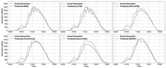
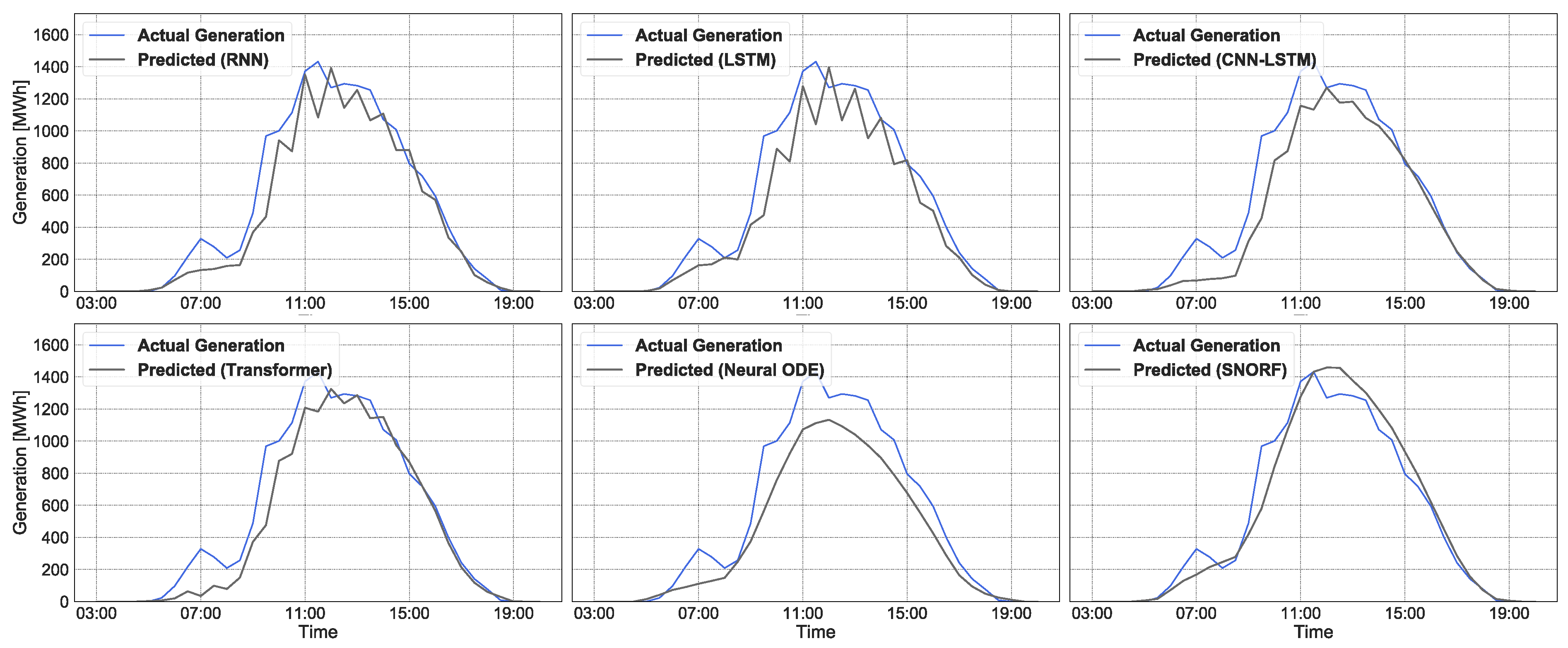
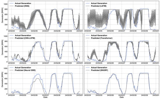
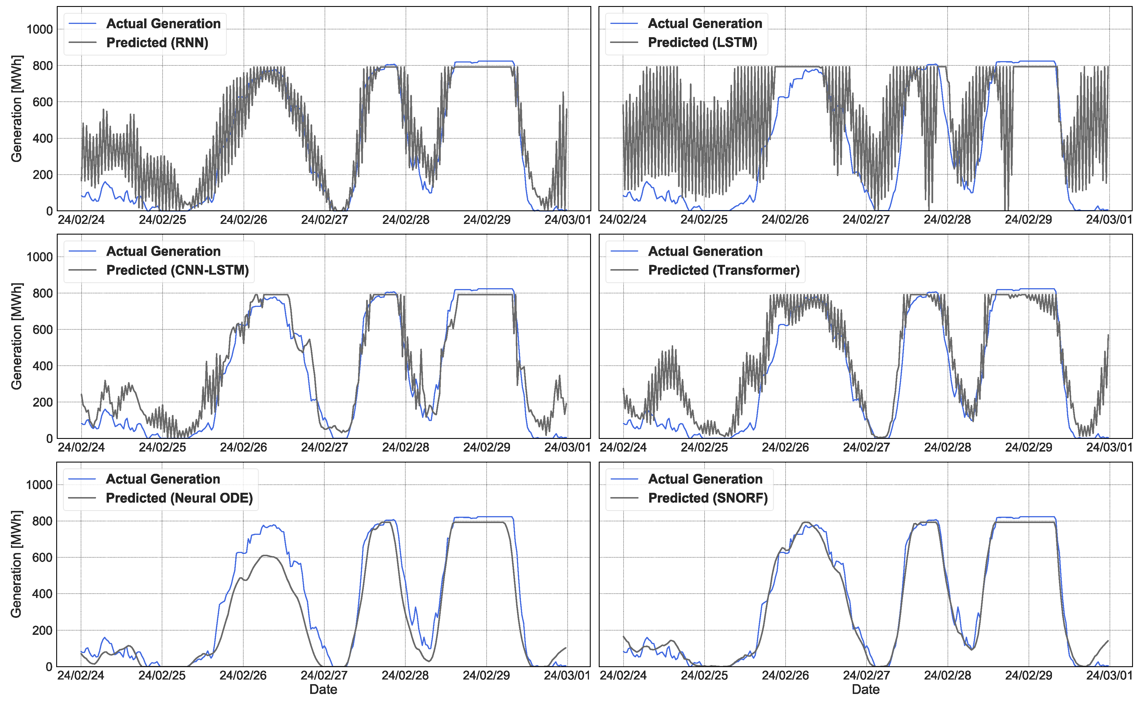
For wind forecasting, the performance gain is more pronounced. SNORF reduces RMSE by 12.09% and MAE by 22.67% relative to the strongest baseline, Neural ODE. Compared with CNN-LSTM and Transformer, the improvements reach 35.04% and 37.36% in RMSE, and 42.92% and 44.91% in MAE, respectively. Compared with RNN and LSTM, the improvements reach 58.80% and 57.50% in RMSE, and 65.90% and 64.00% in MAE, respectively. These results demonstrate SNORF’s ability to produce accurate, efficient, and temporally consistent forecasts under rolling conditions. Representative visual comparisons are shown in Figure 5 and Figure 6.

Figure 5. SNORF and baseline models in solar generation forecasting.

Figure 6. SNORF and baseline models in wind generation forecasting.

5.2. Long-Term Forecasting Performance

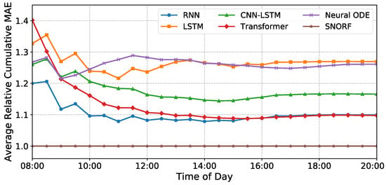
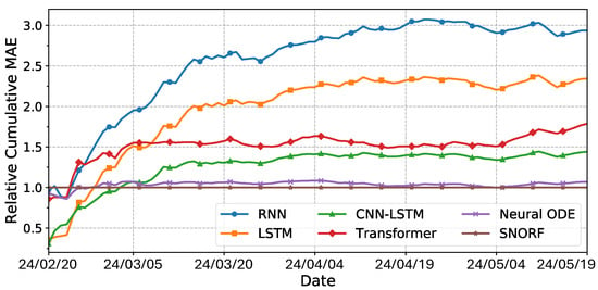
To examine how forecasting errors evolve over extended horizons, we present the relative cumulative MAE trajectories for each model. Rather than plotting absolute cumulative errors, the cumulative MAE of each model is normalized by that of SNORF at each time step, yielding a relative cumulative MAE curve with SNORF serving as the baseline (value = 1). This representation highlights how forecasting errors accumulate over time relative to the SNORF model.

For solar forecasting, since power generation drops to near zero during nighttime, the temporal continuity between consecutive days is weaker than that of wind power. Accordingly, we compute the MAE every 30 min within each day, construct the within-day cumulative error series, and then aggregate the cumulative values corresponding to each clock time across all test dates to obtain the average cumulative MAE profile. In addition, to ensure robustness, the cumulative MAE values are computed using the averaged generation outputs across multiple independent runs.

In contrast, wind generation exhibits more continuous temporal dependencies throughout the day, so we compute daily MAE values and accumulate them sequentially to capture long-term error growth across the evaluation period. Similarly, the cumulative error curves are based on the averaged results over multiple runs. The resulting curves therefore represent relative cumulative errors, enabling direct comparison of how rapidly each model’s forecasting errors accumulate relative to the SNORF baseline.

As shown in Figure 7 and Figure 8, SNORF serves as the reference baseline, while most competing models exhibit relative cumulative MAE values above 1 for substantial portions of the evaluation horizon, indicating faster cumulative error growth than SNORF. In some intervals, certain baseline models temporarily fall below the SNORF baseline, reflecting lower cumulative errors over those partial periods. However, across the full evaluation horizon, SNORF maintains the most favorable long-term error accumulation behavior.

Figure 7. Average relative cumulative MAE by time of day for solar forecasts.

Figure 8. Relative cumulative MAE over the evaluation period for wind forecasts.

This improved behavior can be attributed to the architectural design of SNORF. Specifically, the bounded drift function constrains the magnitude of hidden-state updates, preventing abrupt transitions that may amplify prediction errors. In addition, the repeated Euler-based integration enforces gradual and smooth hidden-state evolution, which acts as a low-pass filter on high-frequency variations. Together, these mechanisms limit the propagation and accumulation of errors during recursive forecasting, resulting in more stable long-horizon predictions. Overall, these results indicate that SNORF provides more robust long-horizon forecasting performance under recursive rolling prediction compared with conventional deep learning models for time-series forecasting.

5.3. Benchmarking Against HEFTcom24 Winners

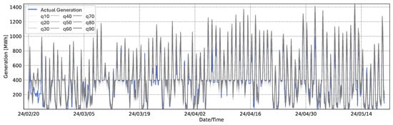
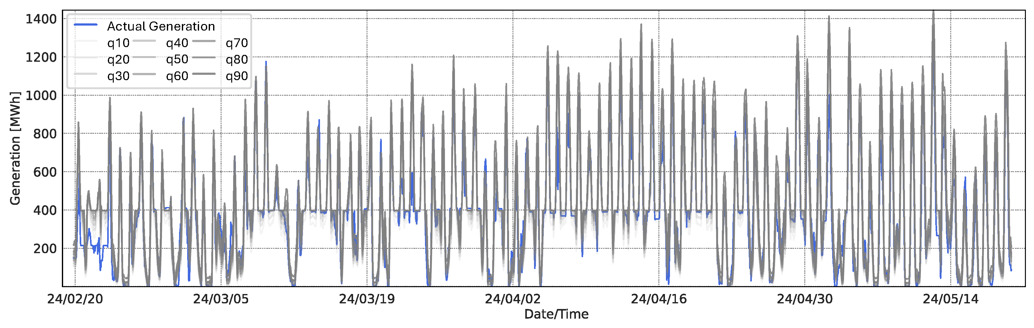
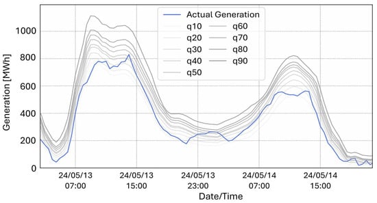
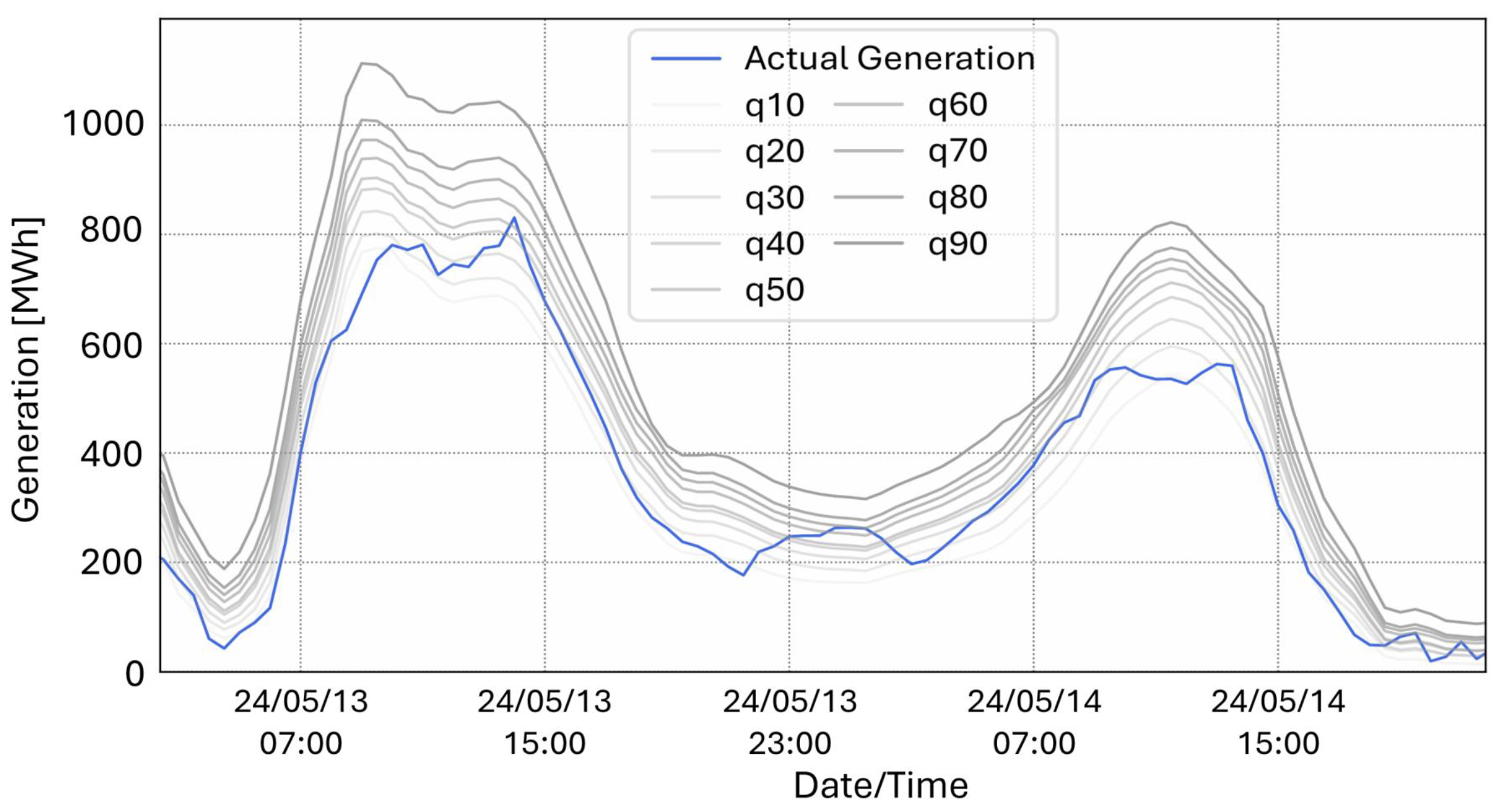
To align with the official HEFTcom24 evaluation protocol, we assessed SNORF using nine quantile levels. Figure 9 presents quantile predictions over the entire test period, while Figure 10 illustrates representative quantile predictions on selected test days. Based on the competition’s official evaluation, SNORF achieved a final Pinball Score of 23.85 MWh, ranking third overall and placing within the top 4% of all participating teams.

Figure 9. Quantile predictions over the entire HEFTcom24 test period.

Figure 10. Representative quantile predictions on the HEFTcom24 test set.

SNORF was evaluated under the official HEFTcom24 protocol and dataset for comparison purposes, although it was not an official competition submission. Table 9 summarizes the scores and methodologies of the top-performing participants in the HEFTcom24 competition [31]. Several high-ranking teams relied heavily on high-resolution meteorological data and sophisticated ensemble techniques to improve their forecasts. For instance, SVK leveraged CatBoost models with MEPS data, UI×BUD employed LightGBM ensembles with manual correction strategies, and Rnt used proprietary weather data in conjunction with Transformer-based architectures. In contrast, SNORF achieved top-tier forecasting performance without any additional datasets or post-processing techniques, using only the officially provided DWD dataset. This strong performance stems from two core factors. First, the rolling forecasting framework enabled effective future prediction even in data-limited environments by feeding the model’s own outputs back as inputs. Second, and more critically, SNORF’s architectural design, featuring an input-dependent bounded drift function and repeated Euler-based integration, successfully suppressed oscillatory behavior and stabilized predictions, addressing the inherent instability of rolling forecasts.

Table 9. Comparison of top-performing teams in HEFTcom24. N/A indicates that the method was not an official competition submission.

Rank	Team	PS	Used Method
1	SVK	22.18	CatBoost stacking, MEPS
2	UI·BUD	23.18	LightGBM per quantile, manual tuning
N/A	SNORF	23.85	Rolling forecast using SNORF
3	Rnt	24.64	Transformer, Reint AI weather model
4	GEB	25.16	LightGBM, numerical convolution

5.4. Ablation Study

To better understand the contribution of the key architectural components of SNORF, we conducted an ablation study isolating the effects of the bounded drift function and repeated Euler integration. Specifically, four model variants were evaluated: (1) the full SNORF model with both components enabled, (2) a model without bounded drift, (3) a model without repeated Euler integration, and (4) a model without both components. For fairness and to ensure robustness of the results, each experiment was repeated 10 times with different random initializations, and the mean and standard error were reported. The results for solar and wind forecasting are summarized in Table 10 and Table 11, respectively.

Table 10. Ablation study of the proposed solar SNORF model components. Values are presented as mean ± SE. An asterisk (*) indicates SE values rounded to 0.00 due to their small magnitude. A checkmark (✓) indicates that the corresponding component is included in the model.

Bounded Drift	Repeated Euler	RMSE (%) ± SE	MAE (kWh) ± SE	PCC ± SE
✓	✓	6.12 ± 0.07	61.99 ± 0.69	0.97 ± 0.00 *
	✓	7.87 ± 0.35	80.48 ± 3.75	0.96 ± 0.00 *
✓		7.69 ± 0.55	79.89 ± 5.78	0.96 ± 0.00 *
		11.65± 0.60	110.91± 5.71	0.92 ± 0.01

Table 11. Ablation study of the proposed wind SNORF model components. Values are presented as mean ± SE. A checkmark (✓) indicates that the corresponding component is included in the model.

Bounded Drift	Repeated Euler	RMSE (%) ± SE	MAE (kWh) ± SE	PCC ± SE
✓	✓	21.08 ± 0.76	112.59 ± 4.99	0.87 ± 0.01
	✓	22.83 ± 1.53	136.36 ± 12.20	0.87 ± 0.01
✓		24.45 ± 1.79	144.95 ± 11.31	0.83 ± 0.02
		32.29 ± 4.65	203.23 ± 33.44	0.73 ± 0.06

For solar forecasting, the full SNORF model achieves the best performance across all metrics. Removing either the bounded drift or the repeated Euler integration leads to a noticeable degradation in accuracy, with both variants showing similar performance drops. When both components are removed, the performance deteriorates substantially, indicating that these two mechanisms jointly play a critical role in stabilizing hidden-state dynamics and mitigating error accumulation during recursive forecasting. Overall, the results suggest that both bounded drift and repeated Euler integration contribute meaningfully and synergistically in the solar setting.

For wind forecasting, the same overall pattern is observed, with the full SNORF model achieving the best performance and the model without both components showing the largest degradation. However, compared to the solar case, the relative contributions of the two components differ. Removing the bounded drift function results in a performance degradation, although the extent of the degradation remains relatively limited. In contrast, removing the repeated Euler integration causes a more consistent degradation across all evaluation metrics. This suggests that, for wind forecasting, repeated Euler integration plays a more prominent role in improving predictive performance, whereas the contribution of bounded drift is comparatively smaller, although still beneficial overall.

The relatively smaller gains in the wind forecasting task can be attributed to both the intrinsic characteristics of wind power generation and the experimental configuration. Wind power exhibits higher variability and weaker temporal continuity compared to solar power, making it less dependent on smooth temporal evolution of hidden states. In addition, the wind model was trained with a timestep of 1, which reduces the extent of recursive dependency across time. As a result, the stabilizing mechanisms designed to control recursive error propagation have a diminished effect. Nevertheless, when both components are removed, the performance drops significantly, suggesting that they still play a complementary role in maintaining overall model robustness.

These observations are broadly consistent with the theoretical stability perspective discussed earlier. The bounded drift formulation constrains the magnitude of hidden-state updates, while repeated Euler integration encourages gradual temporal evolution. Although their individual contributions may vary depending on the dataset and temporal structure, their combination helps limit abrupt hidden-state transitions and suppress cumulative error growth during recursive forecasting. The empirical results in Table 10 and Table 11 support this interpretation, showing that SNORF achieves stable long-horizon predictions by structurally regularizing hidden-state dynamics.

6. Discussion

SNORF achieves stable and accurate rolling forecasts by structurally mitigating error amplification without relying on post hoc smoothing. This stability is primarily attributed to two key mechanisms: bounded hidden-state updates and gradual temporal evolution.

• Euler-based incremental updates: Hidden states evolve through small incremental steps, effectively acting as a low-pass filter on hidden dynamics. With bounded tanh activation and time step $\Delta t$, the update magnitude is constrained:

  $$|h_{t+1}-h_t|\le \Delta t\times C.$$

  (10)
  This suppresses high-frequency oscillations during recursive prediction.
• Bounded drift function: The drift function $f(h_t,x_t)$ is bounded, limiting hidden-state variation and reducing error amplification. Under the Lipschitz assumption, prediction error satisfies

  $$|e_{t+1}|\le L\times |e_t|.$$

  (11)
  Although $L<1$ is not explicitly enforced, bounded activations and small $\Delta t$ help prevent uncontrolled error growth (see Appendix A).

Together, these mechanisms enforce smooth hidden-state dynamics across recursive steps, making stability an intrinsic architectural property. The number of Euler unfolding steps provides a practical trade-off between smoothness and model flexibility. Empirically, SNORF consistently improves both predictive accuracy and temporal coherence across datasets, while maintaining strong performance under limited meteorological inputs. However, real-world renewable energy systems involve additional operational constraints (e.g., curtailment and grid limits) that are only partially considered in this study, suggesting an avenue for future work.

SNORF also has several limitations. Performance depends on the choice of $\Delta t$, which controls hidden-state update magnitude. Repeated Euler updates introduce modest computational overhead, although overall complexity remains comparable to recurrent models. Because the computational complexity scales linearly with the sequence length, the proposed framework is well-suited for higher-resolution datasets with finer temporal granularity. Future work will extend SNORF to more complex nonlinear energy systems and incorporate richer operational constraints.

7. Conclusions

This study proposed SNORF, a neural ODE-based forecasting architecture designed to improve stability and accuracy in rolling time-series prediction. By structurally constraining hidden-state dynamics, SNORF mitigates the error amplification commonly observed in recursive forecasting. Unlike many existing approaches that rely on high-resolution meteorological inputs or post-processing techniques, the proposed model achieves stable long-horizon forecasting using only basic meteorological variables and lagged generation data.

The main findings of this study can be summarized as follows:

• SNORF introduces a structurally stable rolling forecasting architecture by combining an input-dependent bounded drift function with repeated Euler-based integration.
• The proposed architecture suppresses oscillatory behavior and limits error accumulation during recursive prediction.
• Experimental results on solar and wind generation datasets demonstrate that SNORF consistently outperforms representative time-series forecasting models in terms of RMSE, MAE, and temporal consistency.
• When evaluated under the official HEFTcom24 protocol, SNORF achieves a top 4% ranking using only the basic weather dataset, highlighting its robustness in data-constrained forecasting environments.

Despite these promising results, several limitations remain. The forecasting performance is moderately influenced by the choice of the Euler time step $\Delta t$, which controls the magnitude of incremental hidden-state updates. In addition, although repeated Euler updates improve stability, they introduce a modest computational overhead compared with a single recurrent update. Furthermore, operational constraints such as curtailment policies or detailed turbine operating conditions were not explicitly modeled in this study.

Because SNORF uses fixed-step updates rather than adaptive ODE solvers, the computational complexity scales linearly with sequence length, making the framework suitable for higher-resolution datasets. Future work will further evaluate the model using higher-frequency renewable generation data. In addition, future research will investigate the applicability of SNORF to a broader range of nonlinear energy systems.

Appendix B.1. Information on the Solar Dataset

Table A1. Summary of the solar power forecasting dataset used in this study.

Parameters	Details
Provided by	Hybrid Energy Forecasting and Trading Competition
Organization	Deutscher Wetterdienst
Time Resolution	30 min
Location	England
Available Features	Solar radiation, relative humidity, cloud cover, Installed solar capacity
Used Features	Time, generation (30, 60, 90 min prior), Installed solar capacity, temperature diff, cloud cover, radiation
Dataset Splits	Training: 20 September 2020–19 February 2024; Test: 20 February 2024–19 May 2024

Table A1. Summary of the solar power forecasting dataset used in this study.

Parameters	Details
Provided by	Hybrid Energy Forecasting and Trading Competition
Organization	Deutscher Wetterdienst
Time Resolution	30 min
Location	England
Available Features	Solar radiation, relative humidity, cloud cover, Installed solar capacity
Used Features	Time, generation (30, 60, 90 min prior), Installed solar capacity, temperature diff, cloud cover, radiation
Dataset Splits	Training: 20 September 2020–19 February 2024; Test: 20 February 2024–19 May 2024

Appendix B.2. Information on the Wind Dataset

Table A2. Summary of the wind power forecasting dataset used in this study.

Parameters	Details
Provided by	Hybrid Energy Forecasting and Trading Competition
Organization	Deutscher Wetterdienst
Time Resolution	30 min
Location	England
Available Features	Wind speed (10 m, 100 m), wind direction (10 m, 100 m), relative humidity
Used Features	Time, temperature, generation (30, 60, 90 min prior), wind speed 100m (0, 30, 60 min prior), wind direction
Dataset Splits	Training: 20 September 2020–19 February 2024; Test: 20 February 2024–19 May 2024

Table A2. Summary of the wind power forecasting dataset used in this study.

Parameters	Details
Provided by	Hybrid Energy Forecasting and Trading Competition
Organization	Deutscher Wetterdienst
Time Resolution	30 min
Location	England
Available Features	Wind speed (10 m, 100 m), wind direction (10 m, 100 m), relative humidity
Used Features	Time, temperature, generation (30, 60, 90 min prior), wind speed 100m (0, 30, 60 min prior), wind direction
Dataset Splits	Training: 20 September 2020–19 February 2024; Test: 20 February 2024–19 May 2024

Appendix C.1. RNN Parameters for Solar Forecasting

Table A3. Hyperparameter configuration of the RNN model for solar forecasting.

Parameter	Value	Range	Method
Time Step	4	[1, 30]	Discrete (step = 1)
Hidden size	48	[32, 256]	Uniform
Linear hidden size	189	[32, 256]	Uniform
SAM $\rho$	0.0176	[0.01, 0.1]	Uniform
Dropout	0.0764	[0.0, 0.5]	Uniform
Learning Rate	0.0028	[${10}^{-4}$, ${10}^{-2}$]	Log-uniform
Batch Size	128	[64, 128, 256]	Categorical

Table A3. Hyperparameter configuration of the RNN model for solar forecasting.

Parameter	Value	Range	Method
Time Step	4	[1, 30]	Discrete (step = 1)
Hidden size	48	[32, 256]	Uniform
Linear hidden size	189	[32, 256]	Uniform
SAM $\rho$	0.0176	[0.01, 0.1]	Uniform
Dropout	0.0764	[0.0, 0.5]	Uniform
Learning Rate	0.0028	[${10}^{-4}$, ${10}^{-2}$]	Log-uniform
Batch Size	128	[64, 128, 256]	Categorical

Appendix C.2. RNN Parameters for Wind Forecasting

Table A4. Hyperparameter configuration of the RNN model for wind forecasting.

Parameter	Value	Range	Method
Time Step	27	[1, 30]	Discrete (step = 1)
Hidden size	89	[32, 256]	Uniform
Linear hidden size	241	[32, 256]	Uniform
SAM $\rho$	0.0263	[0.01, 0.1]	Uniform
Dropout	0.0668	[0.0, 0.5]	Uniform
Learning Rate	0.0015	[${10}^{-4}$, ${10}^{-2}$]	Log-uniform
Batch Size	64	[64, 128, 256]	Categorical

Table A4. Hyperparameter configuration of the RNN model for wind forecasting.

Parameter	Value	Range	Method
Time Step	27	[1, 30]	Discrete (step = 1)
Hidden size	89	[32, 256]	Uniform
Linear hidden size	241	[32, 256]	Uniform
SAM $\rho$	0.0263	[0.01, 0.1]	Uniform
Dropout	0.0668	[0.0, 0.5]	Uniform
Learning Rate	0.0015	[${10}^{-4}$, ${10}^{-2}$]	Log-uniform
Batch Size	64	[64, 128, 256]	Categorical

Appendix C.3. LSTM Parameters for Solar Forecasting

Table A5. Hyperparameter configuration of the LSTM model for solar forecasting.

Parameter	Value	Range	Method
Time Step	21	[1, 30]	Discrete (step = 1)
Hidden size	210	[32, 256]	Uniform
Linear hidden size	206	[32, 256]	Uniform
SAM $\rho$	0.0178	[0.01, 0.1]	Uniform
Dropout	0.1959	[0.0, 0.5]	Uniform
Learning Rate	0.0060	[${10}^{-4}$, ${10}^{-2}$]	Log-uniform
Batch Size	64	[64, 128, 256]	Categorical

Table A5. Hyperparameter configuration of the LSTM model for solar forecasting.

Parameter	Value	Range	Method
Time Step	21	[1, 30]	Discrete (step = 1)
Hidden size	210	[32, 256]	Uniform
Linear hidden size	206	[32, 256]	Uniform
SAM $\rho$	0.0178	[0.01, 0.1]	Uniform
Dropout	0.1959	[0.0, 0.5]	Uniform
Learning Rate	0.0060	[${10}^{-4}$, ${10}^{-2}$]	Log-uniform
Batch Size	64	[64, 128, 256]	Categorical

Appendix C.4. LSTM Parameters for Wind Forecasting

Table A6. Hyperparameter configuration of the LSTM model for wind forecasting.

Parameter	Value	Range	Method
Time Step	29	[1, 30]	Discrete (step = 1)
Hidden size	152	[32, 256]	Uniform
Linear hidden size	228	[32, 256]	Uniform
SAM $\rho$	0.0253	[0.01, 0.1]	Uniform
Dropout	0.1081	[0.0, 0.5]	Uniform
Learning Rate	0.0027	[${10}^{-4}$, ${10}^{-2}$]	Log-uniform
Batch Size	64	[64, 128, 256]	Categorical

Table A6. Hyperparameter configuration of the LSTM model for wind forecasting.

Parameter	Value	Range	Method
Time Step	29	[1, 30]	Discrete (step = 1)
Hidden size	152	[32, 256]	Uniform
Linear hidden size	228	[32, 256]	Uniform
SAM $\rho$	0.0253	[0.01, 0.1]	Uniform
Dropout	0.1081	[0.0, 0.5]	Uniform
Learning Rate	0.0027	[${10}^{-4}$, ${10}^{-2}$]	Log-uniform
Batch Size	64	[64, 128, 256]	Categorical

Appendix C.5. CNN-LSTM Parameters for Solar Forecasting

Table A7. Hyperparameter configuration of the CNN-LSTM model for solar forecasting.

Parameter	Value	Range	Method
Time Step	21	[1, 30]	Discrete (step = 1)
CNN Filters	64	[16, 128]	Discrete (step = 16)
CNN Kernel	3	[1, time step]	Uniform
Hidden size	210	[32, 256]	Uniform
Linear hidden size	206	[32, 256]	Uniform
SAM $\rho$	0.0178	[0.01, 0.1]	Uniform
Dropout	0.1959	[0.0, 0.5]	Uniform
Learning Rate	0.0060	[${10}^{-4}$, ${10}^{-2}$]	Log-uniform
Batch Size	64	[64, 128, 256]	Categorical

Table A7. Hyperparameter configuration of the CNN-LSTM model for solar forecasting.

Parameter	Value	Range	Method
Time Step	21	[1, 30]	Discrete (step = 1)
CNN Filters	64	[16, 128]	Discrete (step = 16)
CNN Kernel	3	[1, time step]	Uniform
Hidden size	210	[32, 256]	Uniform
Linear hidden size	206	[32, 256]	Uniform
SAM $\rho$	0.0178	[0.01, 0.1]	Uniform
Dropout	0.1959	[0.0, 0.5]	Uniform
Learning Rate	0.0060	[${10}^{-4}$, ${10}^{-2}$]	Log-uniform
Batch Size	64	[64, 128, 256]	Categorical

Appendix C.6. CNN-LSTM Parameters for Wind Forecasting

Table A8. Hyperparameter configuration of the CNN-LSTM model for wind forecasting.

Parameter	Value	Range	Method
Time Step	27	[1, 30]	Discrete (step = 1)
CNN Filters	96	[16, 128]	Discrete (step = 16)
CNN Kernel	2	[1, time step]	Uniform
Hidden size	185	[32, 256]	Uniform
Linear hidden size	158	[32, 256]	Uniform
SAM $\rho$	0.0178	[0.01, 0.1]	Uniform
Dropout	0.1747	[0.0, 0.5]	Uniform
Learning Rate	0.0009	[${10}^{-4}$, ${10}^{-2}$]	Log-uniform
Batch Size	64	[64, 128, 256]	Categorical

Table A8. Hyperparameter configuration of the CNN-LSTM model for wind forecasting.

Parameter	Value	Range	Method
Time Step	27	[1, 30]	Discrete (step = 1)
CNN Filters	96	[16, 128]	Discrete (step = 16)
CNN Kernel	2	[1, time step]	Uniform
Hidden size	185	[32, 256]	Uniform
Linear hidden size	158	[32, 256]	Uniform
SAM $\rho$	0.0178	[0.01, 0.1]	Uniform
Dropout	0.1747	[0.0, 0.5]	Uniform
Learning Rate	0.0009	[${10}^{-4}$, ${10}^{-2}$]	Log-uniform
Batch Size	64	[64, 128, 256]	Categorical

Appendix C.7. Transformer Parameters for Solar Forecasting

Table A9. Hyperparameter configuration of the Transformer model for solar forecasting.

Parameter	Value	Range	Method
Time Step	3	[1, 30]	Discrete (step = 1)
d_model (d_m)	32	[16, 128]	Discrete (step = 16)
ff_dim	32	[d_m, 4*d_m]	Discrete (step = d_m)
n_heads	2	[1, 2, 4, 8]	Categorical
SAM $\rho$	0.0204	[0.01, 0.1]	Uniform
Dropout	0.4151	[0.0, 0.5]	Uniform
Learning Rate	0.0035	[${10}^{-4}$, ${10}^{-2}$]	Log-uniform
Batch Size	64	[64, 128, 256]	Categorical

Table A9. Hyperparameter configuration of the Transformer model for solar forecasting.

Parameter	Value	Range	Method
Time Step	3	[1, 30]	Discrete (step = 1)
d_model (d_m)	32	[16, 128]	Discrete (step = 16)
ff_dim	32	[d_m, 4*d_m]	Discrete (step = d_m)
n_heads	2	[1, 2, 4, 8]	Categorical
SAM $\rho$	0.0204	[0.01, 0.1]	Uniform
Dropout	0.4151	[0.0, 0.5]	Uniform
Learning Rate	0.0035	[${10}^{-4}$, ${10}^{-2}$]	Log-uniform
Batch Size	64	[64, 128, 256]	Categorical

Appendix C.8. Transformer Parameters for Wind Forecasting

Table A10. Hyperparameter configuration of the Transformer model for wind forecasting.

Parameter	Value	Range	Method
Time Step	11	[1, 30]	Discrete (step = 1)
d_model (d_m)	96	[16, 128]	Discrete (step = 16)
ff_dim	192	[d_m, 4*d_m]	Discrete (step = d_m)
n_heads	4	[1, 2, 4, 8]	Categorical
SAM $\rho$	0.0178	[0.01, 0.1]	Uniform
Dropout	0.4658	[0.0, 0.5]	Uniform
Learning Rate	0.0053	[${10}^{-4}$, ${10}^{-2}$]	Log-uniform
Batch Size	128	[64, 128, 256]	Categorical

Table A10. Hyperparameter configuration of the Transformer model for wind forecasting.

Parameter	Value	Range	Method
Time Step	11	[1, 30]	Discrete (step = 1)
d_model (d_m)	96	[16, 128]	Discrete (step = 16)
ff_dim	192	[d_m, 4*d_m]	Discrete (step = d_m)
n_heads	4	[1, 2, 4, 8]	Categorical
SAM $\rho$	0.0178	[0.01, 0.1]	Uniform
Dropout	0.4658	[0.0, 0.5]	Uniform
Learning Rate	0.0053	[${10}^{-4}$, ${10}^{-2}$]	Log-uniform
Batch Size	128	[64, 128, 256]	Categorical

Appendix C.9. Neural ODE Parameters for Solar Forecasting

Table A11. Hyperparameter configuration of the Neural ODE model for solar forecasting.

Parameter	Value	Range	Method
Input type	Pointwise	–	–
Hidden size	249	[32, 256]	Uniform
Linear hidden size	267	[32, 256]	Uniform
SAM $\rho$	0.0398	[0.01, 0.1]	Uniform
Dropout	0.3689	[0.0, 0.5]	Uniform
ODE solver	Odeint	–	–
Learning Rate	0.0040	[${10}^{-4}$, ${10}^{-2}$]	Log-uniform
Batch Size	256	[64, 128, 256]	Categorical

Table A11. Hyperparameter configuration of the Neural ODE model for solar forecasting.

Parameter	Value	Range	Method
Input type	Pointwise	–	–
Hidden size	249	[32, 256]	Uniform
Linear hidden size	267	[32, 256]	Uniform
SAM $\rho$	0.0398	[0.01, 0.1]	Uniform
Dropout	0.3689	[0.0, 0.5]	Uniform
ODE solver	Odeint	–	–
Learning Rate	0.0040	[${10}^{-4}$, ${10}^{-2}$]	Log-uniform
Batch Size	256	[64, 128, 256]	Categorical

Appendix C.10. Neural ODE Parameters for Wind Forecasting

Table A12. Hyperparameter configuration of the Neural ODE model for wind forecasting.

Parameter	Value	Range	Method
Input type	Pointwise	–	–
Hidden size	68	[32, 256]	Uniform
Linear hidden size	392	[32, 256]	Uniform
SAM $\rho$	0.0068	[0.01, 0.1]	Uniform
Dropout	0.3488	[0.0, 0.5]	Uniform
ODE solver	Odeint	–	–
Learning Rate	0.0052	[${10}^{-4}$, ${10}^{-2}$]	Log-uniform
Batch Size	256	[64, 128, 256]	Categorical

Table A12. Hyperparameter configuration of the Neural ODE model for wind forecasting.

Parameter	Value	Range	Method
Input type	Pointwise	–	–
Hidden size	68	[32, 256]	Uniform
Linear hidden size	392	[32, 256]	Uniform
SAM $\rho$	0.0068	[0.01, 0.1]	Uniform
Dropout	0.3488	[0.0, 0.5]	Uniform
ODE solver	Odeint	–	–
Learning Rate	0.0052	[${10}^{-4}$, ${10}^{-2}$]	Log-uniform
Batch Size	256	[64, 128, 256]	Categorical

References

- Zhao, C.; Li, X. A novel real-time energy management strategy for gird-friendly microgrid: Harnessing internal fluctuation internally. In Proceedings of the 2020 52nd North American Power Symposium (NAPS), Tempe, AZ, USA, 11–13 April 2021; IEEE: Piscataway, NJ, USA, 2021; pp. 1–6. [Google Scholar]
- Peng, D.; Lee, S.; Choi, S. Renewable-Integrated agent-based microgrid model with grid-forming support for improved frequency regulation. Mathematics 2025, 13, 3142. [Google Scholar] [CrossRef] [Scilit]
- Sheng, L.; Fu, N.; Mou, J.; Zhu, L.; Zhou, J. Data-Driven Probabilistic Wind Power Forecasting and Dispatch with Alternating Direction Method of Multipliers over Complex Networks. Mathematics 2025, 14, 112. [Google Scholar] [CrossRef] [Scilit]
- Diesing, P.; Bogdanov, D.; Keiner, D.; Satymov, R.; Toke, D.; Breyer, C. Exploring the demand for inter-annual storage for balancing wind energy variability in 100% renewable energy systems. Energy 2024, 312, 133572. [Google Scholar] [CrossRef] [Scilit]
- Yoo, Y.; Jung, S. Modeling forecast errors for microgrid operation using Gaussian process regression. Sci. Rep. 2024, 14, 2166. [Google Scholar] [CrossRef] [Scilit]
- Fan, C.; Zhang, Y.; Pan, Y.; Li, X.; Zhang, C.; Yuan, R.; Wu, D.; Wang, W.; Pei, J.; Huang, H. Multi-horizon time series forecasting with temporal attention learning. In Proceedings of the 25th ACM SIGKDD International Conference on Knowledge Discovery & Data Mining, Anchorage, AK, USA, 4–8 August 2019; pp. 2527–2535. [Google Scholar]
- Sun, Y.; Li, S.; Lin, B.; Fu, X.; Ramezani, M.; Jaithwa, I. Artificial neural network for control and grid integration of residential solar photovoltaic systems. IEEE Trans. Sustain. Energy 2017, 8, 1484–1495. [Google Scholar] [CrossRef] [Scilit]
- Saxena, N.; Kumar, R.; Rao, Y.K.; Mondloe, D.S.; Dhapekar, N.K.; Sharma, A.; Yadav, A.S. Hybrid KNN-SVM machine learning approach for solar power forecasting. Environ. Challenges 2024, 14, 100838. [Google Scholar] [CrossRef] [Scilit]
- Park, M.K.; Lee, J.M.; Kang, W.H.; Choi, J.M.; Lee, K.H. Predictive model for PV power generation using RNN (LSTM). J. Mech. Sci. Technol. 2021, 35, 795–803. [Google Scholar] [CrossRef] [Scilit]
- Xia, M.; Shao, H.; Ma, X.; De Silva, C.W. A stacked GRU-RNN-based approach for predicting renewable energy and electricity load for smart grid operation. IEEE Trans. Ind. Inform. 2021, 17, 7050–7059. [Google Scholar] [CrossRef] [Scilit]
- Ayman-Mursaleen, M.; Saeed, S.T.; Almohammadi, S.M.; Arif, K.; Imran, M. A deep neural network model for heat transfer in darcy–forchheimer hybrid nanofluid flow with activation energy. Sci. Rep. 2026, 16, 8339. [Google Scholar] [CrossRef] [Scilit]
- Krishnamurthy, N.K.; Pandey, A.K.; Rao, S.S. Machine learning based annual solar energy forecasting for enhanced grid integration of photovoltaic systems. Bull. Electr. Eng. Inform. 2025, 14, 4267–4278. [Google Scholar] [CrossRef] [Scilit]
- Rajasundrapandiyanleebanon, T.; Kumaresan, K.; Murugan, S.; Subathra, M.; Sivakumar, M. Solar energy forecasting using machine learning and deep learning techniques. Arch. Comput. Methods Eng. 2023, 30, 3059–3079. [Google Scholar] [CrossRef] [Scilit]
- Fu, K.; Guo, Y.; Qiu, W. Optimization of Microgrid Scheduling Based on Adaptive Collaborative Secretary Bird Optimization Algorithm. Mathematics 2026, 14, 622. [Google Scholar] [CrossRef] [Scilit]
- Yang, H.; Wang, H.; Gao, Y.; Liu, X.; Xu, M. A significant wave height forecast framework with end-to-end dynamic modeling and lag features length optimization. Ocean Eng. 2022, 266, 113037. [Google Scholar] [CrossRef] [Scilit]
- Caljon, D.; Vercauteren, J.; De Vos, S.; Verbeke, W.; Van Belle, J. Using dynamic loss weighting to boost improvements in forecast stability. arXiv 2024, arXiv:2409.18267. [Google Scholar] [CrossRef] [Scilit]
- Sun, Y.; Zhao, X.; Dai, H.; Wang, F.; Feng, G. A Medium-term Daily Electricity Consumption Rolling Multi-step Forecasting Method Considering Meteorologically Similar Days. In Proceedings of the 2025 IEEE Industry Applications Society Annual Meeting (IAS), Taipei, Taiwan, 5–20 June 2025; IEEE: Piscataway, NJ, USA, 2025; pp. 1–8. [Google Scholar]
- Yu, L.; Ma, Y.; Ma, M. An effective rolling decomposition-ensemble model for gasoline consumption forecasting. Energy 2021, 222, 119869. [Google Scholar] [CrossRef] [Scilit]
- Yang, S.; Vinuesa, R.; Kang, N. Towards Robust Spatio-Temporal Auto-Regressive Prediction: Adams-Bashforth Time Integration with Adaptive Multi-Step Rollout. arXiv 2024, arXiv:2412.05657. [Google Scholar]
- Jauregui-Correa, J.C. Forecasting the dynamic response of rotating machinery under sudden load changes. Machines 2023, 11, 857. [Google Scholar] [CrossRef] [Scilit]
- Pu, W.; Xie, Y.; Zhao, Z.; Hong, C.; Shi, H.; Fan, Y.; Lu, Y.; Han, D.; Ye, J.; Yan, X.; et al. Research on high proportion of clean energy grid-connected oscillation risk prediction technology based on CNN and trend feature analysis. Sci. Rep. 2023, 13, 22149. [Google Scholar] [CrossRef] [Scilit]
- Dejonckheere, J.; Disney, S.M.; Lambrecht, M.R.; Towill, D.R. Transfer function analysis of forecasting induced bullwhip in supply chains. Int. J. Prod. Econ. 2002, 78, 133–144. [Google Scholar] [CrossRef] [Scilit]
- Godahewa, R.; Bergmeir, C.; Webb, G.I.; Hyndman, R.J.; Montero-Manso, P. Monash time series forecasting archive. arXiv 2021, arXiv:2105.06643. [Google Scholar] [CrossRef] [Scilit]
- Zhang, J.; Hua, Y.; Xue, Z.; Song, T.; Zheng, C.; Ma, R.; Guan, H. Robust Bayesian neural networks by spectral expectation bound regularization. In Proceedings of the the IEEE/CVF Conference on Computer Vision and Pattern Recognition, Virtual Event, 19–25 June 2021; pp. 3815–3824. [Google Scholar]
- Akiba, T.; Sano, S.; Yanase, T.; Ohta, T.; Koyama, M. Optuna: A next-generation hyperparameter optimization framework. In Proceedings of the 25th ACM SIGKDD International Conference on Knowledge Discovery & Data Mining, Anchorage, AK, USA, 4–8 August 2019; pp. 2623–2631. [Google Scholar]
- Foret, P.; Kleiner, A.; Mobahi, H.; Neyshabur, B. Sharpness-aware minimization for efficiently improving generalization. arXiv 2020, arXiv:2010.01412. [Google Scholar]
- Browell, J.; Haglund, S.; Kälvegren, H.; Simioni, E.; Bessa, R.; Wang, Y.; van der Meer, D. Hybrid Energy Forecasting and Trading Competition. IEEE DataPort 2023. [Google Scholar] [CrossRef]
- Mudiyanselage, M.W.; Wu, H.; Mehrabidavoodabadi, A. Multivariant Short-Term Residential Load Forecasting with Dual Path Trigonometric Encoding LSTM and Attention Mechanism. In Proceedings of the 2024 International Symposium on Electrical, Electronics and Information Engineering (ISEEIE), Leicester, UK, 28–30 August 2024; IEEE: Piscataway, NJ, USA, 2024; pp. 450–456. [Google Scholar]
- Imani, M.; Ghassemian, H. Lagged load wavelet decomposition and LSTM networks for short-term load forecasting. In Proceedings of the 2019 4th International Conference on Pattern Recognition and Image Analysis (IPRIA), Tehran, Iran, 6–7 March 2019; IEEE: Piscataway, NJ, USA, 2019; pp. 6–12. [Google Scholar]
- Menze, B.H.; Kelm, B.M.; Masuch, R.; Himmelreich, U.; Bachert, P.; Petrich, W.; Hamprecht, F.A. A comparison of random forest and its Gini importance with standard chemometric methods for the feature selection and classification of spectral data. BMC Bioinform. 2009, 10, 213. [Google Scholar] [CrossRef] [Scilit] [PubMed]
- Browell, J. HEFTcom Leaderboard Announcement. In Proceedings of the IEEE Power and Energy Society, Seattle, WA, USA, 21–25 July 2024. [Google Scholar]
Disclaimer/Publisher’s Note: The statements, opinions and data contained in all publications are solely those of the individual author(s) and contributor(s) and not of MDPI and/or the editor(s). MDPI and/or the editor(s) disclaim responsibility for any injury to people or property resulting from any ideas, methods, instructions or products referred to in the content. |
© 2026 by the authors. Licensee MDPI, Basel, Switzerland. This article is an open access article distributed under the terms and conditions of the Creative Commons Attribution (CC BY) license.