


Abstract
It has been shown in several works that a population dispersing in a heterogeneous habitat can reach a higher density than it would get if dispersal was not allowed or if space was homogeneous. Those previous works have extended and completed the study of this phenomenon and the conditions under which it occurs, but mainly using very specific models. In the present paper, we propose a more general extension based on a very large class of models, among which the previous ones belong. Furthermore, we propose a framework based on a time scale separation method to illustrate that the previous class of models may also include more complex ones. We illustrate this framework on two examples based on mass balanced equations, a resource–consumer system in a two patch habitat and a resource–consumer–predator system in a two patch habitat. In each case, we show how our general approach allows us to determine explicit conditions under which the above mentioned phenomenon is occurring. It is note worthy that our conditions extend the well-known conditions discovered in the previous works. We think that this robust result may be of strong interest for environmental management for fragmented habitats.
MSC:
92D25; 92D40
1. Introduction
Space is known as a crucial ingredient to explain population variability as described in very abundant literature. In this paper, we focus on a particular phenomenon that has been highlighted in [1]. In that work, the authors show that under specific assumptions, a population living in a two patch habitat having each a given carrying capacity when taken in isolation, can reach a total abundance larger that the sum of the local carrying capacities. This total abundance reached on the whole multi-patch habitat is now referred to the TRAPA (Total Reached Asymptotic Population Abundance) after [2]. From those works, we know that dispersal in a heterogeneous habitat may lead the population to a higher abundance than what it would get in the absence of dispersal or in a homogenous environment. Since we will often mention this phenomenon in this paper, we call it DIG (for Dispersal Induced Growth) as suggested in [3] who found a similar phenomenon in time-periodic systems. DIG occurring in heterogeneous space (as done in this work) could cover many applications, because it implies that habitat fragmentation may reduce the population productivity. The assumptions made in [1] are that the local growth on each patch is governed by a logistic growth model and that the dispersion is symmetrical, meaning that the dispersion rates from one patch to the other one are equal. The authors also assumed that the dispersion is much faster than the local growth. They provide an explicit relationship between the total population abundance at equilibrium and the sum of local carrying capacities. This allows us to understand explicitly the conditions under which the DIG phenomenon occurs.
Since that work, many papers have extended and generalized the results. In [4], the author considers a population in a heterogeneous environment represented with an arbitrary number of patches and the local growth rate is not explicitly given. He shows that dispersal has a stabilizing effect but does not consider the DIG phenomenon. In [5], the author provides a graphical approach to generalize the result of [1] to a broad class of models where the per capita growth rate on each patch is not specified but still in the case of symmetrical dispersal. The case where it is a logistic growth model is just dealt with as an example. Furthermore, the author provides what is called the rule because it provides the condition on the parameters and on each patch under which the DIG phenomenon takes place. Note that refs. [1,5] discuss their results in the context of the evolutionary role of dispersal, this process having been shown selected against in [6]. In [7], the authors consider the asymmetrical case and extend the results. Asymmetry allows for the consideration of a more general situation because symmetry is a very specific hypothesis. Ref. [7] provides an explicit relationship between the local carrying capacities and the TRAPA assuming fast dispersal and shows that the TRAPA can be larger than the sum of local carrying capacities even when noise is included, which ensures some robustness of this phenomenon. An application of this work to the study of a predator-prey system in a patchy environment is given in [8]. Many other extensions have been proposed among which the case with more patches in [9], with continuous space and PDEs in [10], models with discrete time in [11], models of harvested populations in [12,13,14] and so on.
Concerning the specific logistic growth model on two patches, ref. [15] (see Proposition 1 and Proposition 2) provides a complete mathematical analysis of the dynamics and the conditions under which the TRAPA is higher than the sum of the local carrying capacities in the case of symmetrical dispersal. These conditions extend the rule. Ref. [16] extends further the results to the asymmetric dispersal case with a geometrical description of the dynamics in the phase space which is very enlightening. That last paper shows that the model has a unique globally asymptotically stable equilibrium and adds accurate conditions under which the rule also extends. In [17], the authors extend the results of [16] providing more information on the conditions under which the DIG occurs for the logistic model on two patches. In [18] the authors analyse in details the impact of asymmetrical dispersal rates on the TRAPA using a local logistic growth model. It must also be noted that a more mechanistic model has been proposed in [19], where the author proposes a specific resource–consumer system and shows that the DIG phenomenon can also happen in this case. Another interesting case concerns density dependent dispersal rates. In [20], the author studies the DIG phenomenon in a multi-patch system with local logistic growth and density dependent dispersal. Interestingly, all these theoretical works have found some experimental supports as can be seen in [2], where the authors designed an experiment to test the DIG phenomenon and the conditions under which it can be observed. Note that ref. [15] shows that their result is also valid for a system where the population growth is not given by a logistic model, but includes an explicit resource. This more mechanistic approach is very important because the concept of carrying capacity has been the subject of several debates ([21] for instance). However, it must be noticed that the mechanistic model given in [15] is strictly equivalent to the standard logistic growth model from a mathematical point of view. Recent works extend the analysis of the role of the dispersal intensity on the TRAPA, but focusing on the shape of the relationship between dispersal intensity and TRAPA, with no explicit mention to the DIG phenomenon, see for instance [22] for some specific time discrete models, or [23] for a more general formulation of the local growth rate (still time discrete model) or [24] for a model including Allee effect. We also refer to [25] for a study with a continuous time model, where the authors either use a local logistic growth model, or a more mechanistic resource–consumer model, and dispersal between two patches. They use a graphical approach to analyse the interplay between dispersal and spatial heterogeneity.
In the present work, we focus on the DIG phenomenon. We show that this phenomenon can occur for a very general class of growth models. It follows that our results generalize those presented in [16] by extending and adapting the same approach. It must be noted that a more important generalization to any number of patches has been the object of the paper [26]. This paper contains several interesting results among which the existence and unicity of a globally stable positive equilibrium of a generalized growth model in a multi-patch environment (see Theorem 6, p. 917 in [26]), obtained by using the theory of cooperative systems. The paper also considers the TRAPA and provides conditions under which the TRAPA is lower (Proposition 13, p. 922) or higher (Proposition 14, p. 923) than the sum of local carrying capacities (DIG phenomenon). However, we think that there are some problems with the statement and the proof of Proposition 14 in [26], as we discuss later. Thus, this is still an open problem to know under which conditions the DIG phenomenon occurs in a multi-patch system. This is the main objective of this work. A second important aim is to illustrate how this result can be used to study more mechanistic mass balanced models and to understand why and when the spatial heterogeneity and dispersal induce enhanced biomass production. Mechanistic models presented in this work take explicit resource into account. They explain the intra-specific competition underlying the logistic growth model. As it has been discussed in many works (see [27] for a review), this mechanistic approach provides interesting enlightenment on the processes involved in competition and mainly when considering evolutionary consequences of growth in competitive conditions. We want to highlight that dispersal can also decrease the TRAPA (see [28], for example), but it is a somehow more intuitive result than the DIG phenomenon. We also provide some conditions on the dispersal rates under which this TRAPA reduction is obtained in the present work.
First, in Section 2, we consider a population model living in a heterogeneous habitat composed of two different patches. The local growth model is not specified, we only make general assumptions. Dispersal can be asymmetric. No assumption on characteristic time scales is made. We remind the reader that there is a globally asymptotically stable equilibrium and we provide general conditions under which the DIG phenomenon occurs. In the case where the local growth is governed by a logistic growth, our conditions reduce to the previous rule; thus, they are actually a generalization of the conditions given in [16]. In Section 3, we consider a consumer population on a two patch habitat, on which resources are explicitly represented. We assume that the consumer can disperse between the patches and that the resource dynamics are much faster than the consumer dynamics. This establishes a general framework based on Quasi-Steady State Assumption (QSSA) that can be used to build a simpler model of a population growing in a heterogeneous habitat, but the obtained formulation is not the usual logistic growth model. Using the results of the first part, we can provide conditions under which the DIG phenomenon takes place. The approach can be used to study other types of models based on the same general assumptions. Finally, in Section 4, a more complete resource–consumer–predator model is proposed and the same general framework based on QSSA allows us to get conditions under which the DIG phenomenon can be observed. Our work shows that the phenomenon discovered by [1] is very general and can be found in more mechanistic models. We think that it is important because we can interpret the generalization of the rule on the basis of more realistic parameters, having a clear biological or ecological interpretation which can be measured explicitly. The paper ends with a discussion of our results and some perspectives.
2. Growth in a Patchy Environment
We consider here a very general growth model in a patchy environment. The model reads as follows:
where is the population density in patch i, , at time t, (resp. ) is the displacement rate from patch 1 to patch 2 (resp. from patch 2 to patch 1). is the per capita growth rate of the population in patch i and we make now some general assumptions on the functions :
H1:
is a strictly decreasing function on for ,
H2:
there exists such that for ,
H3:
(this assumption is done without loss of generality).
is called the carrying capacity of patch i, that is the maximal density of the population below which the per capita growth rate is positive and above which the growth rate becomes negative when the patch i is isolated (without displacement).
With these notations, we know that if we impede the displacements, then the total number of individuals in the whole domain will be . Note that if we work with densities, we have to take into account patch areas. In order to simplify the text, we assume here that both patches have the same area.
In this section, we will first show that under a given condition on the carrying capacities, there exists movement rates that induce the DIG phenomenon. It, thus, proves that this phenomenon can be observed in a large class of models, but it does not specify the movement rates and it does not provide a relationship between the carrying capacities and the movement rates that lead to the DIG phenomenon. Adding another assumption on the function , we then provide a result that gives an explicit relationship between the movement rates and the carrying capacities so that when this relation is fulfilled, the DIG phenomenon occurs. First of all, we ensure that speaking about TRAPA in our case is meaningful.
Let us consider the positive domain ; we can state our first result, which is a special case of Theorem 6 in [26].
Proposition 1.
System (1) leaves the positive domain invariant. Moreover, it has a unique positive equilibrium, which is globally asymptotically stable.
The proof in [26] uses the theory of monotone systems. In Appendix A, we provide proof for two patches, which may be helpful for a deep understanding of the reason why this result is true. Indeed, in this special case, we can plot the phase space and see explicitly how the vector field is.
Since we know that system (1) has a unique, positive, global and asymptomatic stable equilibrium, we analyze the condition under which the TRAPA encompasses the sum of the local carrying capacities. We denote the equilibrium by and the TRAPA by . Our first result in this direction is the following:
Proposition 2.
Under the same assumptions as before, if , then there exists a range of values for the parameters and of system (1) such that the equilibrium of this system satisfies .
This result claims that the DIG phenomenon can be observed in any model satisfying assumptions and , because assumption is not restrictive. In order to prove this result, we first show the lemma:
Lemma 1.
If then .
Proof of Lemma 1.
We assume that . We use proof by contradiction, and thus, we also assume that:
Since at equilibrium, one has then and one also has ; thus, . Consequently, one would get , which is in contradiction with . We can, thus, conclude that the inequality (2) is wrong. Accordingly, we proved that and then and , which involves and . The lemma follows. □
We can now prove Proposition 2.
Proof of Proposition 2.
Let us denote F the function defined on by:
As done in [16] for instance, by adding the equations of system (1), we conclude that the equilibria of this system are on the set . Note that is on this set. At this point, the derivative does not vanish. Thus, we can apply the Implicit Function Theorem on an open vicinity U of . There exists a neigborhood V of and a function on U such that for all :
In other words, locally around , the set of equilibria is the graph of . The slope of this graph at is:
where we used . First, this means that is decreasing at this point. Furthermore, using the proposition assumption leads to the conclusion that . We can, thus, conclude that the set of equilibria crosses the straight line (which has a slope equal to ) and enters in the domain when in U. Let us denote by this part of the graph of .
Now, consider the straight line . The equilibrium is located on somewhere between the set and according to Lemma 1. Thus, and are chosen in such a way that the straight line crosses ; we know that and, thus, . This ends the proof. □
Thus, assumptions and ensure that there exists dispersal rates producing the DIG phenomenon. Now we are interested to find a lower bound for the ratio such that if this ratio is larger than this bound, the DIG phenomenon takes place. If possible, we would like to get a bound that is easy to calculate in applications, as done in the next section. However, to get this result we added another assumption:
H4:
for all .
It is easy to check that this assumption is fulfilled by the logistic growth model. Moreover, it is satisfied by the examples dealt with in this work (see next section).
Proposition 3.
With the same notations and assumptions as above, if the following condition is fulfilled:
then .
Before proving this proposition, we need the following lemma. Note that the proof of this lemma is inspired by the proof of Proposition 1 in [15]. Namely, we use a Taylor expansion at the order 2. In [15], there is no remainder because the logistic model is a polynomial of degree 2. Here, we have a remainder in the Taylor expansion and assumption is used to fix the sign of this remainder (we use the Lagrange remainder).
In the proof of Proposition 14 in [26], the author does not make any assumption on and uses a Peano remainder in the Taylor expansion. The remainder is written by using a Landau notation, . However, we do not know that (the equilibrium value of ) is close to and this can even be wrong as we see here. Thus, we can not neglect it and we do not know its sign while the author does not consider this. It is one of the problems of the proof of that proposition. Another issue concerns the use of a notation , which is well defined when the two ratios and are equal. However, the author continues to use this notation when the ratios are not equal, while in this case is not defined. It follows that the statement of Proposition 14 in [26] is not clear and we could not find a way to clarify it. It is the reason why we propose here only the case with two patches instead of n ones.
Lemma 2.
If the condition is fulfilled:
then .
Proof of Lemma 2.
Since, for , is a function, there exists some such that (Taylor–Lagrange formula):
It turns then out that:
and this last equality holds for . Summing these equalities gives:
Now, at equilibrium, one has:
Replacing these expressions in Formula (7) gives:
Since we assumed that , then condition (4) associated to the result of Lemma 1 involves that the first term of the right hand side is strictly positive and the second term is always positive, thus, . □
Proof of Proposition 3.
Finally, we propose a more complete result, but this one requires another assumption. We, thus, consider the assumption:
H5:
for all for .
Which allows us to give a geometrical interpretation of the result and to extend the proof given in [16]. Note also that in the case of the logistic growth model, , thus, . The extra-assumption is satisfied in the case of the logistic model. We can now state our last main result:
Theorem 1.
With the assumptions and notations set above, two cases can be distinguished.
- 1.
- If then .
- 2.
- If then .
Note that the case is not dealt with in Theorem 1. In order to prove this theorem, we introduce some notations and prove two lemmas.
Notations: the set can be divided in four regions denoted by , for and defined as follows:
Let us again (see proof of Proposition 2) consider the map F defined in by . By adding the equations of the model (1), we can conclude that the equilibria of this model are on the set defined by . To understand when the TRAPA is larger than , it is useful to introduce the straight line . Using this set, we can say that the total abundance at equilibrium is larger than if, and only if, the point is located above the straight line in the plane . Since we know that the equilibrium must be located on the set , we will now provide some results that allow us to describe when the set is above or below the line in .
Lemma 3.
With the notations set previously and assuming that in model (1), follows and , then we can conclude that:
- (a)
- contains the points , , , and ;
- (b)
- there exists a function defined on such that and on , is the graph of ;
- (c)
- the graph of is included in ;
- (d)
- there exists a function defined on such that and on , is the graph of .
- (e)
- the graph of is included in ;
- (f)
- .
- (g)
- is a curve which is made of the union .
Proof of Lemma 3.
The proof of item (a) is obvious. Let us prove item (b). First, . Indeed, if , then and, thus, on . This means that , thus, is an empty set.
Let us now consider a point on with and . We have either and then , or and then again , or and then .
Since , then . Thus, for each such , there exists an open neighborhood of , an open neighborhood of and a function such that for each and with then using the Implicit Function Theorem. We consider as many points like this as required to cover the set , which is compact. Thus, there exists a finite number of neighborhoods that recover . Considering the function such that for all and all p in the finite number set mentioned just above, we obtain the required function of item (b). As we have seen, each point of the graph of is in if we restrict to and and , completing the graph with and . This proves item (c). By symmetry of F with respect to and , we can use the same arguments to prove items (d) and (e). Finally, in the set , it is obvious to see that from which item (f) results. By construction, item (g) then follows. □
With this lemma, we can now state the following one.
Lemma 4.
With the same notations and assumptions as in Lemma 1, and still denoting by the graph of for , we have:
- (a)
- The set is convex.
- (b)
- if then is always below in ;
- (c)
- if then is always below in .
Proof of Lemma 4.
Let us start with item [a]. In order to prove it, we will show that for all and that for all and since the curve is (last item of Lemma 3), the result follows. We know from Lemma 3 that:
It follows that:
and consequently:
from which we get:
The numerator of the fraction is strictly negative from assumption (). Since for all , we have . With , we can conclude that the denominator is also strictly negative (using assumption ()). Thus, the ratio is positive and then for all . We can show in the same way that and since the curve is , we can conclude that the domain is convex.
Now, let us prove [b]. From (9), it follows that:
It follows that which is strictly larger than −1 from the assumption of [b]. In other words, the curve (seen as a graph of a function of ) has a slope larger than the slope of at . As a consequence, in a vicinity of , the straight line is above the curve is and below in the other case. Finally, the slope of the tangent of is strictly decreasing for , thus, it is always larger than −1. It follows that the curve is always below the straight line for . Finally, we proceed in the same way to prove item [c]. □
Proof of Theorem 1.
Let us consider the point which is at the intersection of the straight line defined by with the straight line defined by . A straightforward calculation gives:
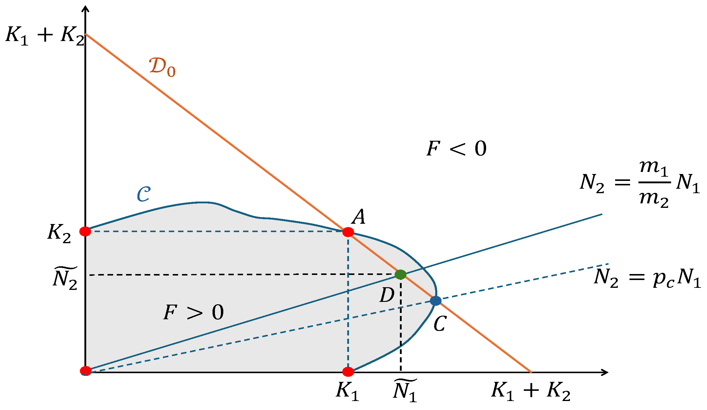
We first prove that condition 1 in Theorem 1 induces that . Consequently, the intersection between the straight line defined by and the curve is in the domain (see Figure 1). Since the equilibrium point is above , it is then also on the part of in the domain (see Figure 1). This proves the result. Then, let us show that . Note that we assume here that , or equivalently . One has:
Figure 1.
This figure illustrates the conditions that allow the DIG phenomenon to occur. It shows how the set of equilibria in the phase space intersects the area where . The orange straight line corresponds to . If the blue continuous straight line is above the blue dashed straight line, then the DIG phenomenon is observed (since we consider , the blue continuous straight line is always below point A.
To prove the second item, first note that is equivalent to say that the slope of the set of equilibria (considered locally at as the graph of ) is lower than , thus, the curve enters the region when becomes larger than because of the convexity of the domain . Since the equilibrium must be in this part of the phase space when from Lemma 4, we get the result. □
In the next section, a mechanistic mass balanced model in which each parameter has a clear biological interpretation is considered. In each patch, we introduce a resource which is consumed by a population that can disperse between the patches. We use the results presented above to understand the fate of the system and to understand if and when the TRAPA can be larger than the total population size that would be reached if the patches were isolated.
3. A Resource–Consumer Model in a Heterogeneous Environment with Different Time Scales
In this section, we present a resource–consumer model in a two patch environment. The aim is to extend the previous results to a mechanistic model in order to analyze the results under the light of parameters that are easier to measure and interpret than the carrying capacity. The model contains four coupled differential equations that represents the dynamics of the resource and consumer on each patch. We use a mathematical result to simplify the model which, at the end, has the same form as system (1). Then we use the previous results to show that the DIG phenomenon is still true here and we provide the conditions under which it occurs. In the first step, we illustrate how a consumer resource model on a homogeneous environment can be simplified into a simpler growth model for the consumer population. In a second step, the resource–consumer is embedded in a two patches environment.
3.1. A Resource–Consumer Model in a Homogeneous Environment
We denote by (resp. ) the resource density (resp. the consumer density) at time . The model reads:
where I is the resource input rate, k is the output rate per unit of mass of resource, a is the consumption rate per unit of mass of resource and consumer, is the conversion efficiency and is the mortality rate of the consumer. is a dimensionless parameter, and we assume that it is a small positive real number meaning that the growth and death of the consumer are much slower than the resource dynamics. We, thus, assume that the resource dynamics are much faster than the consumer dynamics, for instance a characteristic time scale of hours for the resource and days for the consumer. We can, thus, use the so-called quasi steady state assumption, as follows.
Since is small, we consider in a first step that it can be replaced by 0. In this case, C is constant in time. Equation (10a) allows us to conclude that tends to an equilibrium value given by:
when the time increases. Now, is not exactly equal to 0 and, thus, C is not constant, it moves slowly. For each value taken by C, the fast dynamics of R moves this variable to a value close to . Thus, Equation (10b) can be approximated by:
where , and . We, thus, find here the Schoener model [29]. The mathematical proof of this result is very similar to that we do for system (A6) in Appendix B.
Under this form, the Schoener model looks like a logistic growth model, but it has a very different interpretation for the “intrinsic growth rate” . Indeed, since depends on the consumer density, it cannot be considered as an intrinsic growth rate, that is the growth rate that the consumer population should have in absence of density dependence effect. However, the parameter K can be compared to the carrying capacity, that is the maximal population density that the environment can carry when isolated. Note that under the mechanism discussed here, the parameter K is positive only if the input rate is higher than the critical value , the ratio between the product of the system output rates and the consumer production rate. We will not consider the case where here, this would lead to extinction of the consumer population and the resource would reach the value . We always assume in this work that .
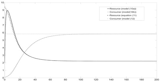
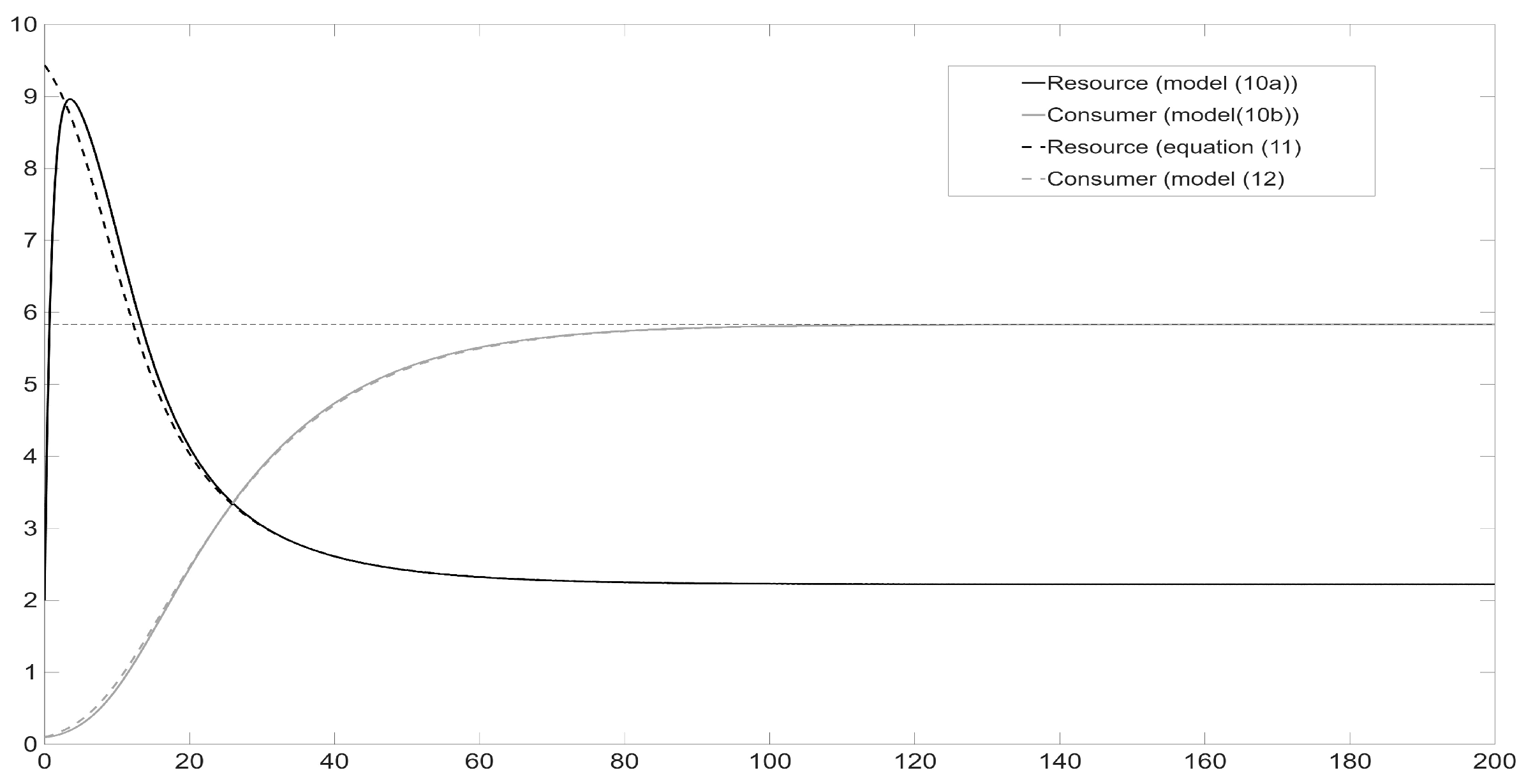
The dynamic is a logistic-like one and the approximation made on the basis of the time scale separation is efficient, as can be seen in Figure 2. Moreover, our simplification also allows us to determine the amount of resource in the environment by using the formula giving .
Figure 2.
This figure compares the dynamics of model (10) versus model (12) for a small value of . The grey curves represent the consumer dynamics and the black curves correspond to the resource dynamics. Continuous curves are obtained with model (10), while dashed curves result from model (12) and Formula (11). The parameters used are , , , , and .
In the next subsection, we extend the method to the study of the resource–consumer system in a patchy environment. For this, it is convenient to introduce the following notation: let f the function defined by . With this notation, model (12) can be written as: . Note also that f is on and strictly decreasing. Furthermore, . Thus, f fulfills the conditions required by functions and in the previous section.
3.2. A Resource–Consumer Model in a Patchy Environment
We can now consider a mechanistic model that accounts explicitly for the resource dynamics in a patchy environment to include spatial heterogeneity and dispersal. The resource represents an abiotic resource in an open environment. Let us make the following assumptions:
- the consumer can move between the patches;
- the dynamics of the resource is faster than the consumer dynamics.
With these assumptions, the model reads:
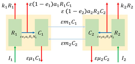
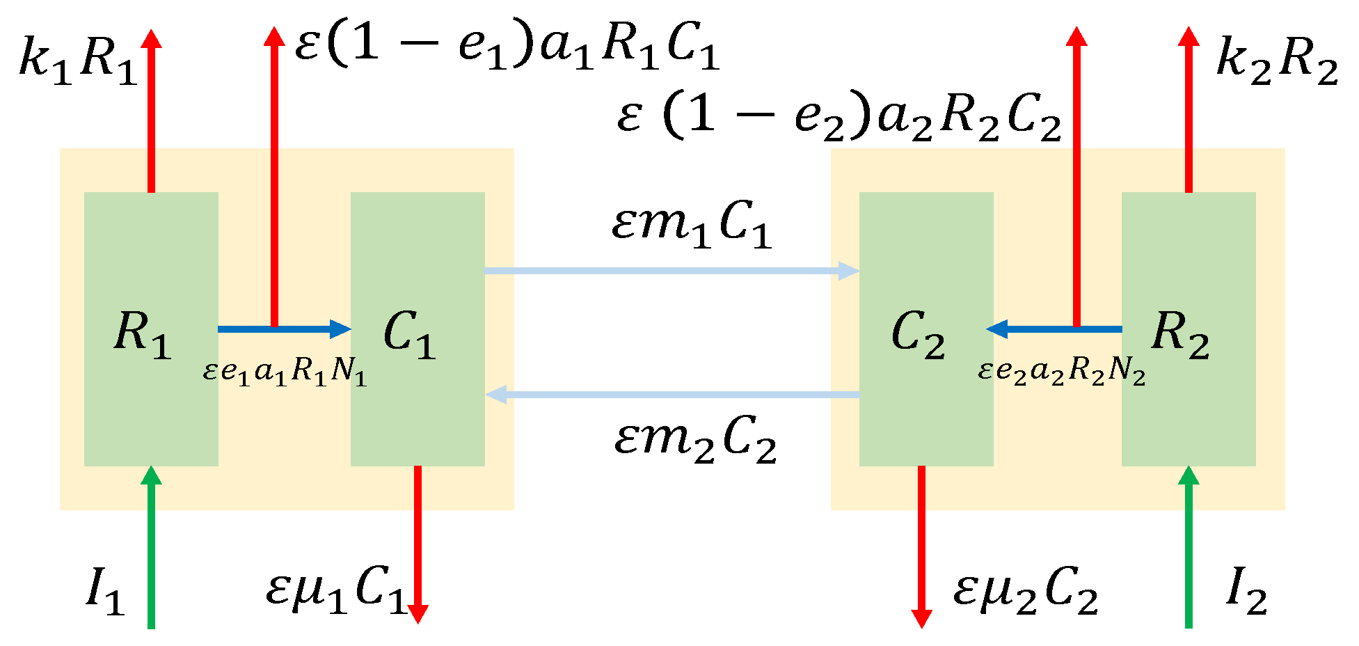
where is the time scale dimensionless parameter, is the input rate of resource , is the output rate of resource per unit of concentration, is the consumption rate of resource by consumer , is the conversion efficiency between resource and consumer , is the mortality rate of consumer , for . (resp. ) is the displacement rate of consumer from patch 1 to patch 2 (resp. from patch 2 to patch 1). Figure 3 summarizes the model and illustrates the flows between the state variables.
Figure 3.
This scheme illustrates the links between the state variables in model (13).
As previously mentioned, using the time scale separation with the QSSA allows us to simplify the model. The mathematical justification used to perform this simplification is based on the Geometrical Singular Perturbation theory introduced by Fenichel ([30,31], see Appendix B). Model (13) can be reduced to the following one:
where for and . We denote by the local carrying capacities (assumed to be positive here), that are the asymtoptic values that subpopulation sizes would reach when the time increases if the patches where isolated by vanishing dispersal rates ( is defined by ). Model (14) can be analyzed by using the previous section and the results allow us to understand model (13). In order to perform this analysis, the condition (3) together with the assumption () must be translated for the resource–consumer case. One gets here , and thus, . With these results, the conditions in (3) read:
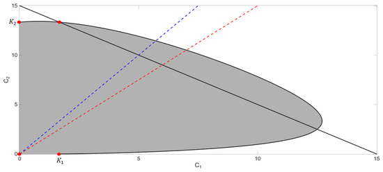
It must be noted, however, that the previous conditions (15) are sufficient conditions to get , but they are not necessary. Not only it is possible to have when the condition is not satisfied, but even more, the larger value of can be reached for parameter values that do not satisfy condition (15). We will see this further in the next section on a more complex model but we can already illustrate this point here with Figure 4 where the phase space is represented with different colors. Note again that the method used here is inspired by [16]. The gray area corresponds to the case where and the white area corresponds to the case where . Thus, the curve between these areas corresponds to , where the equilibria of the model are located. We can see that the points , , and are on this curve (red points). The black straight line corresponds to . The region above this line is, thus, characterized by . The figure shows that the curve crosses the region . If the positive equilibrium point of the model is in this region, the DIG phenomenon is observed.
Figure 4.
This figure illustrates the curve (see main text for details), the boundary of the gray area. The black straight line is defined by , the blue dashed line is defined by and the red dashed line is defined by . The equilibrium point is on the curve and between the blue dashed line and the point . The parameters used for this simulations are , , , , , , and . With these values, and .
We now give a hint to locate the equilibrium point . As is shown in the Appendix A and Appendix B, assuming induces that . This means that the equilibrium point is located between the straight line (blue dashed line on the figure) and the point . We have also seen in the proof of Theorem 1 that if then the intersection between the line and the curve is the region . In other words, means that the straight line is above the straight line (red dashed line on the figure) . Since the gray area is convex, this ensures that the equilibrium point is in the region . However, as can be seen on the figure, even if the blue dashed line is below the black dashed line, it can still cross the curve in the region where , ensuring again that the DIG phenomenon occurs.
In the next section, we consider a more complex model, with a resource–consumer–predator system in a heterogeneous environment and we show that using our framework still allows to get a mathematically tractable model and we can, thus, use the results of the previous section to understand when the DIG phenomenon takes place.
4. A Resource–Consumer–Predator Model in a Heterogeneous Environment with Different Time Scales
In this section, we consider a predator species living on a two patches habitat, and we assume that on each patch, this species feeds on a prey. Thus, on each patch, there is an abiotic resource which is absorbed by a consumer population on which the focal predator population feeds. The predator population can move between patches and we assume that its dynamics is much slower than the resource–consumer dynamics. It can represent a plant–herbivore system for instance, where the plant dynamics are much faster than the herbivore dynamics. The herbivore population can move between the patches. The model reads as follows:
where is the resource concentration on patch i at time , is the consumer density on patch i at time and is the predator density on patch i at time , . and are the resource input rate and the output rate of resource on patch i, I assume that space is heterogeneous, thus, these rates depend on the patch. The parameters a, e, , , and are respectively the absorption rate of resource by the consumer, the growth yield of the consumer, the mortality rate of the consumer, the predation rate, the conversion efficiency and the predator death rate. All of these are biological parameters that are assumed to depend only on the species and, thus, not on the patch. Note that this assumption is not necessary for our results but it has biological explanations and it simplifies the description of the model and results.
Again, is a small positive real number that allows us to represent the time scale separation between resource–consumer dynamics on the one hand and predator dynamics on the other hand. The mathematical treatment of this system is very similar to what is done on the model presented in the previous section. Again, we only give here the heuristic based on the QSSA to understand the dynamics of this six-dimensional system.
At a short time scale (), the predator densities are almost constant and we can focus on only the resource–consumer dynamics. It is straightforward to prove that the system has a unique positive equilibrium which is globally asymptotically stable when it is feasible. This equilibrium reads:
for . This equilibrium is feasible as soon as is lower than the threshold value and we, thus, assume that initially, the predator densities fulfill these conditions for .
At a longer time scale (), the dynamics of the predator are obtained by replacing and by the above equilibrium values and , the model then reads:
where again is the long time scale.
This model has the same form as the general model presented in the first section, where the function can be written as follows:
It is straightforward to show that these functions satisfy the required assumptions of the first section and, thus, the results can be applied. The local carrying capacities are:
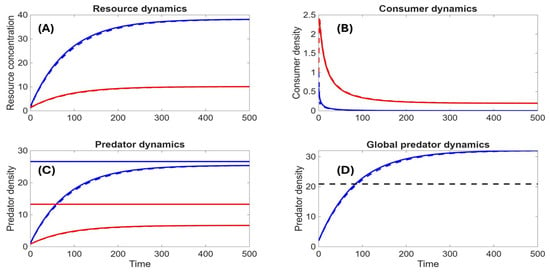
and the required conditions to get these quantities non negative are that for , which is assumed to be true here. Note that , thus, if the patches are isolated, since the predator densities are limited by , the feasibility condition () is satisfied and the reduction of the six-dimensional model (16) to the two-dimensional one (17) is mathematically justified. However, when dispersal is possible, then the predator population can be larger than on a patch which does not guarantee that the reduction is valid. Thus, it must be checked that the reduction is valid if we use the reduced model (17) to understand the complete one (16), as illustrated in Figure 5. This figure shows that both models provide very similar dynamics and then the reduced model can be used to understand the complete one and gives explicit conditions as discussed hereafter. Moreover, on Panel (C) of Figure 5, we can see that indeed, the predator population densities remain below for .
Figure 5.
This figure compares models (16) (continuous lines) to (17) (dashed lines) and shows that the reduced model allows for the understanding of the complete one. Panel (A–C) show respectively the resource, consumer and predator dynamics on each patch (blue = patch 1, red = patch 2). On Panel (C), the horizontal lines show (in blue) and (in red). Panel (D) shows the total number of predators (the blue continuous line is obtained from the complete model while the dashed blue line results from the reduced model), the black dashed horizontal line illustrates the value of . The parameters used for this simulations are , , , , , , , , , , , and .
Now, we can write the conditions (3) for model (16):
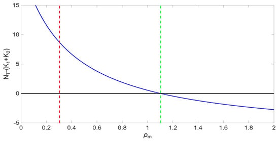
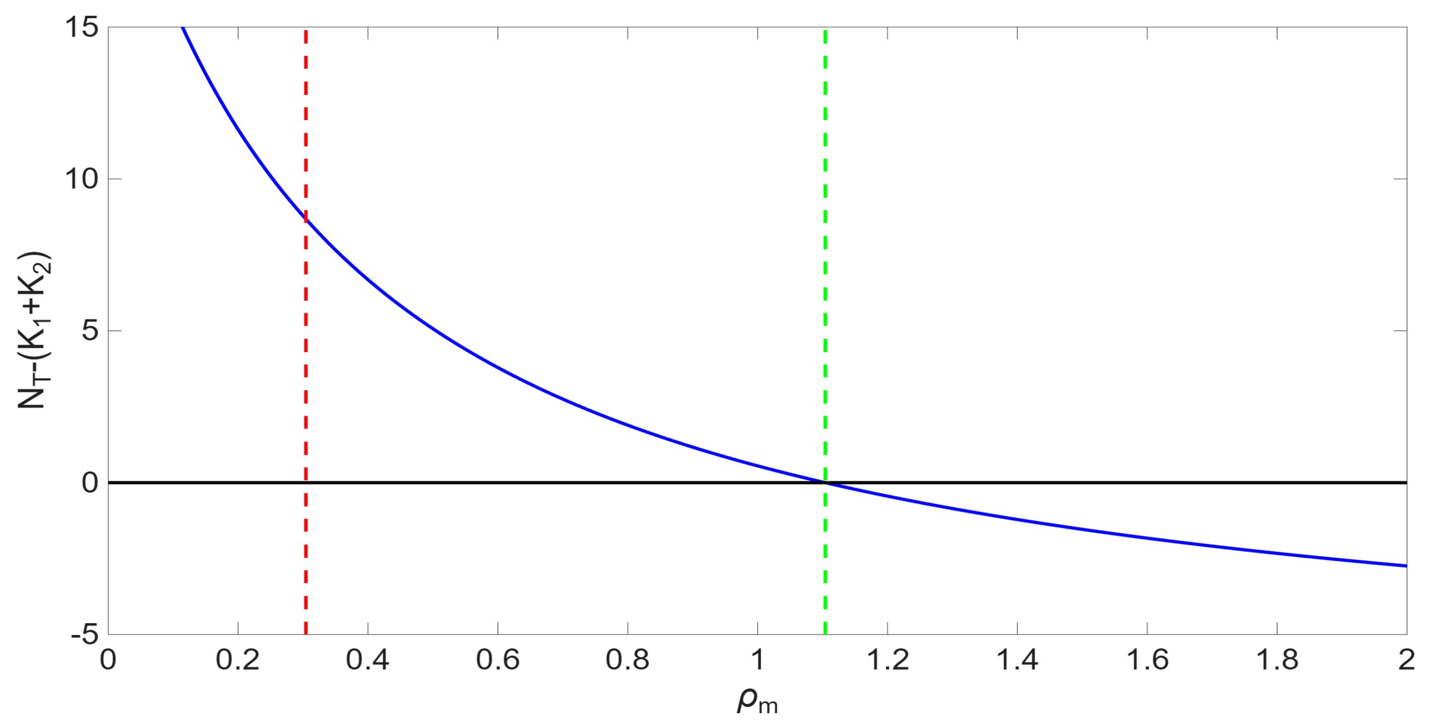
The first section of the paper shows that if these conditions (18) are fulfilled, then the total amount of predators is larger than it would be without dispersal. Again, the left inequality in (18) is a sufficient condition, but even if it is not satisfied, the DIG phenomenon can occur as it can be seen on Figure 6. Indeed, this figure represents the difference between the total number of predators at equilibrium and the sum , as a function of the ratio . The vertical dashed lines of the figure represent the threshold values of given by Formula (18). As we proved in this paper, the DIG phenomenon is always observed between these vertical dashed lines. However, as we can see, it can also be observed for outside of this range, when .
Figure 6.
This figure shows the difference between the Total Realized Asymptotic Population Abundance for system (17) and , for different values of . When the curve is above the horizontal axis , the population reaches a total abundance larger than what it would get in absence of dispersal (DIG phenomenon). The vertical dashed lines represent the threshold of provided by Formula (18). The left vertical red dashed line corresponds to while the right green dashed line illustrates . As shown in the paper, the curve is always above 0 between these thresholds. The parameters used for this simulation are , , , , , , , , , and .
5. Discussion and Conclusions
The aim of this work is two-fold. First, we extend the results of several previous works exhibiting the DIG phenomenon with a logistic equation to a more general model which can cover many particular cases. Second, we use this general result and the framework of Geometrical Singular Perturbation Theory to analyze the DIG phenomenon in details for more realistic but more complex models. Namely, the rule given in the initial work [1] is generalized. We show that the method used in [16] can be extended for a more general formulation. Our results illustrate that the DIG phenomenon is robust and not restricted to a particular model, which can be of interest in the context of structural sensitivity and model uncertainties; see [32] for more details.
Furthermore, we consider mechanistic models in which the population growth results from an explicit resource. We considered two examples to illustrate our approach, but other type of models could also be considered. In each example, using a time scale separation technique, we reduce our complex detailed models with four equations for the resource–consumer model and six equations for the resource–consumer–predator model to a two-dimensional model which has the general form analyzed in the first step. Accordingly, we exhibit conditions under which the DIG phenomenon occurs and these conditions involve meaningful parameters. We, thus, can see the role of each of them. Note that our mechanically based models are mathematically equivalent to a chemostat model. The multi-patch logistic model has been used in previous studies [1,5,7,15] and the form used has been criticised (see [21] for more details). In order to avoid the paradox induced by the logistic growth, ref. [15] proposes a mechanistic approach of the logistic model. Among the solutions, the authors propose a simple resource–consumer model that is mathematically equivalent to the logistic model (Equation (7) in [15]). Thus, the models presented in the present paper are more general, and we could see that they do not lead exactly to a logistic model. Note also that in [15], the authors also considered two mechanistic models. However, the first one is strictly equivalent to the logistic growth equation and the second one includes a logistic equation for the resource and in this sense already contains the weakness that we want to avoid. Moreover, the second example reduces again to the logistic equation, which is again a very particular situation.
Of course, time-scale separation used here needs some assumptions. For instance, it requires that the fast dynamics have a hyperbolically stable equilibrium. This has been checked here and must be checked systematically. Using this method allows us to consider more complex mechanistic models and we only focused on particular situations. For instance, in our models, the local carrying capacities depend explicitly on parameters such as the input rate of nutrient, which controls the nutrient richness of the environment. If this parameter is too low, the values of may become negative. We did not consider this situation here because the paper is focused on the DIG phenomenon. However, in some real situations, this may occur and lead to population extinctions if the input rates are maintained too low during a long period of time. This could not occur with the logistic growth model.
Note that, in order to keep the calculations and explanations as clear and simple as possible, we used linear functional responses for trophic interactions modelling. We checked numerically that the results remain true for Holling type II functional responses and that it was still possible to do our calculations. However, the mathematical expressions were more complex (the fast equilibria for instance are solutions of a second order algebraic equation) and this is why we only show the results for the Holling type I functional responses. Again, however, regarding the robustness of the DIG phenomenon, it is interesting to note that we can generalize this to other types of functional responses.
Finally, we focused in our paper on population dynamics in a patchy environment. It remains a topic of interest if we consider that movement between different patches in a fragmented habitat can have complex and still unknown consequences on population extinction or persistence (see [33] for instance). Moreover, based on previous works like [6] and others, we consider that our results may be analysed in the context of dispersal evolution. We expect to go further in this direction in a future work. As discussed in [27], using mechanistic models for studying the effect of evolution in competing populations is enlightening. We expect that our approach will be helpful when including the evolution of dispersal in mechanistic models.
Author Contributions
Conceptualization, J.-C.P.; Methodology, J.-C.P.; Formal analysis, J.-C.P. and M.G.; Investigation, J.-C.P. and M.G.; Writing—original draft, J.-C.P. and M.G.; Writing—review and editing, J.-C.P. and M.G. All authors have read and agreed to the published version of the manuscript.
Funding
This research received no external funding.
Data Availability Statement
The original contributions presented in this study are included in the article. Further inquiries can be directed to the corresponding author.
Acknowledgments
This work has been inspired by a talk given by Donald L. DeAngelis in Leicester; we want to thank him for this talk and the mail exchanges we get about this problem. The first author wants also to acknowledge Alan Hastings and Vincent Jansen for their comments that led to providing new ideas to go further with our results. The authors also want to acknowledge two anonymous reviewers who made strongly helpful comments on a previous version of this work.
Conflicts of Interest
The authors declare no conflicts of interest.
Appendix A
In this appendix, we give a proof of Proposition 1. We remind the reader that this proposition has more general proof in [26]. The proof here allows us to explicitly take advantage of the two-dimensional system to draw the dynamics in the phase space and see how the dynamics are organized.
Proof of Proposition 1.
As when , it follows that is invariant under the flow of system (1).
We now prove the existence of a positive equilibrium by showing that the isoclines intersect exactly once in the interior of . An equilibrium is a solution of the system:
We now give some notations to define the isoclines. We denote by the function defined by for all and in the same way, for all . The isoclines are, thus, the curves of equations and . Four cases can be distinguished according to the position of with respect to , for . We prove in detail one case and show that all other cases lead to similar situations.
- Case 1: and
From , we get that for all because is decreasing and, thus, for all . Furthermore, since
we can conclude that is strictly increasing on the set . Now, let us consider the straight line . The curve of the function crosses at exactly two points: and . This is straightforward by solving the equation . Additionally, since , it follows that between 0 and , is below while it is above when .
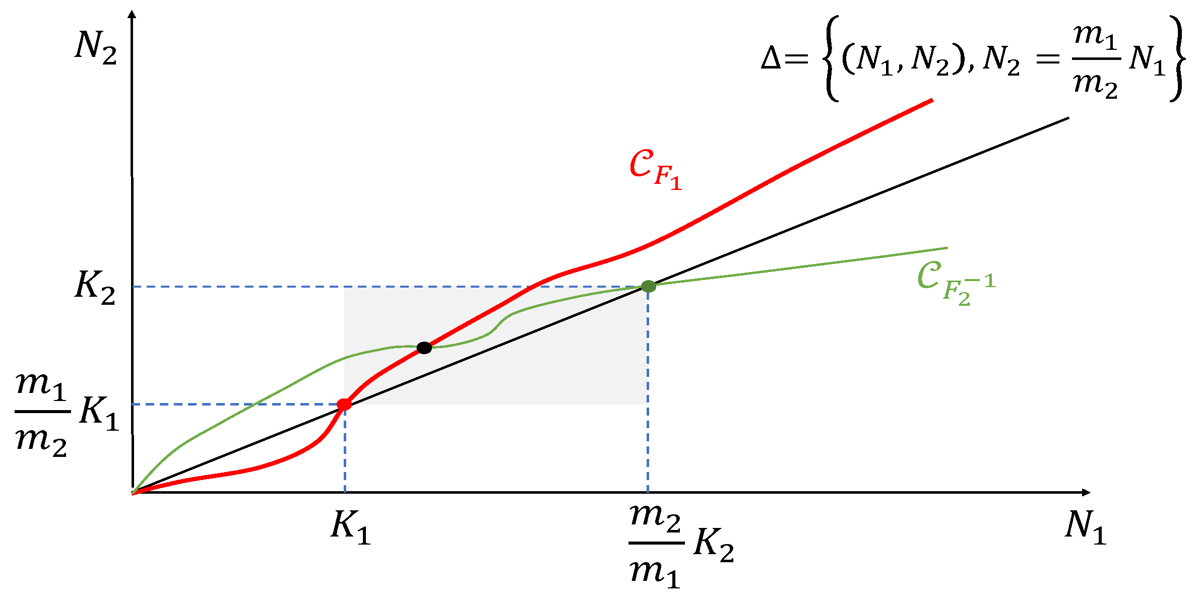
In the same way, we can prove that is a strictly increasing function for . Thus, there exists a function , which is also strictly increasing. The curve is the symmetrical image of the curve of with respect to the diagonal . Note also that crosses at exactly two points: and . With the same arguments used for , we can conclude that the curve is above for all between 0 and while it is below once . Using the third assumption of our statement, we conclude that and of course . All these results are summarized in Figure A1. It follows that the curve is always above the curve for and below for all . Since they are continuous, they cross each other at least once. Thus, at least one positive equilibrium exists for our system. Let us denote by the coordinates of such a positive equilibrium. We know that .
Figure A1.
This figure illustrates the isoclines of system (1). It is shown in the text that at least one equilibrium (black dot) takes place in the grey rectangle and that all positive equilibria must belong to this rectangle.
- Case 2: and
In this case, the isocline starts in the region when is positive and small. We have and . Since is strictly decreasing, there exists a unique such that , meaning that . Moreover, when , ; thus, the curve enters the positive domain at and everywhere increases in this domain, as in the previous case. The proof of this case is now exactly based on the same arguments as in case 1.
- Case 3: and –Case 4: and
We can use the same arguments as in cases 1 and 2 to show that at least a positive equilibrium exists and that its coordinate must belong to .
- Unicity of the positive equilibrium
In order to prove the unicity, we first note that if several positive equilibria exist, their number is odd because of the relative position of the curves at and at . We order the equilibria according to the order of their coordinate (the first one is the one at left in the phase space). At the first one, the isocline crosses and the slope of the isocline is higher than the slope of the isocline. The opposite situation occurs at the second equilibrium and so on. Let us calculate the slopes of the isoclines at equilibrium. We consider any positive equilibrium . We have:
In the same way:
and, thus:
Putting the first and last inequalities together yields:
This last inequality means that at each equilibrium, the slope of the isocline is lower than the slope of the isocline, which is not possible and leads to a contradiction when considering several equilibria. Thus, only one positive equilibrium exists.
- Stability of the positive equilibrium
It is straightforward to show that the Jacobian matrix of the system at its positive equilibrium has a strictly positive determinant and a strictly negative trace. Thus, the positive equilibrium is hyperbolic and locally asymptotically stable. Considering the negative Dulac criterion with the function allows to conclude that the divergence is everywhere strictly negative in the positive domain (interior of ), which, thus, does not contain any limit cycle. We, thus, shall show now that the only possible -limit for each point in the strictly positive domain (interior of ) is the positive equilibrium.
Let us consider the sets defined below:
and
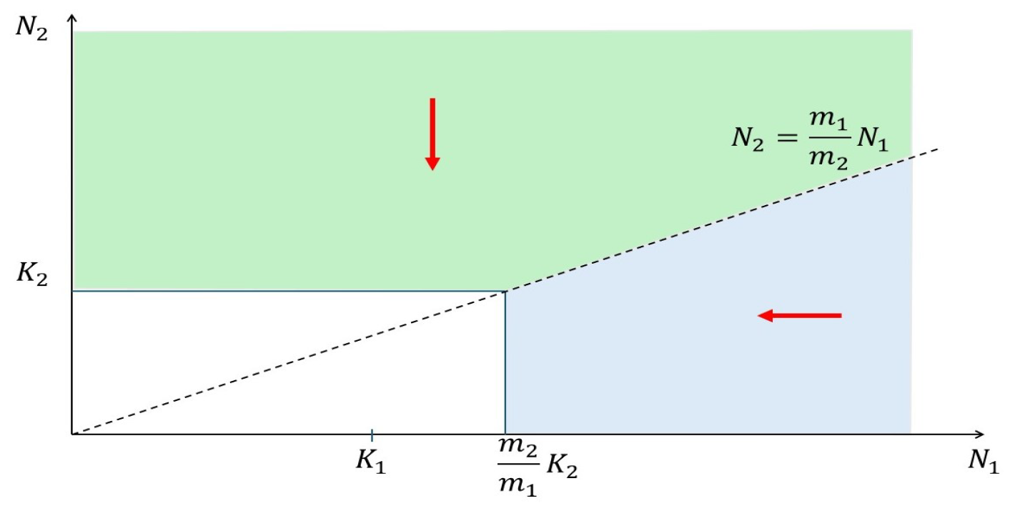
The Figure A2 illustrates these sets and how the dynamics is outside them. For each point outside the set , the vertical component of the vector field is strictly negative, thus, the vector field is pointing downward. It follows that the -limits of these points are in . In the same way, for each point outside the set , the horizontal component of the vector field is strictly negative, thus, the vector field is pointing leftward. As a consequence, the -limits of these points are in . It, thus, turns out that all the -limit sets are in the intersection . This set contains two equilibria: and . Since is a hyperbolically unstable node, it can not belong to the -limit set of any point in the strictly positive domain.
Figure A2.
This figure illustrates the sets (outside the green area) and (outside the blue area). The vector field in the green area points downward and it points leftward in the blue area. Thus, any points in the strictly positive domain have their -limit set in the white rectangle.
Finally, the Poincaré–Bendixon theorem allows us to conclude that the positive equilibrium is the only possible -limit set of any trajectory starting in the strictly positive domain and is, thus, globally asymptotically stable. □
Appendix B
In this appendix, we aim to detail the mathematical material that we used in Section 3 and Section 4 to prove that the reduced models provide the dynamics of the complete models. We do this using a resource–consumer system on two spatial patches as an example. We assume that the consumer can move between patches. Assuming also that the dynamics of a resource are much faster than the dynamics of the consumer, we prove that the system can be reduced to a simpler model satisfying the assumptions of system (1). We, thus, can use the results of Section 2 to understand how the TRAPA can be higher than the sum of local “carrying capacities” in this more mechanistic model.
The resource–consumer model reads:
where is a small parameter meaning that we assume the resource dynamics faster than the consumer dynamics. This model is called a slow–fast system because there are state variables that are much faster than other state variables (see [34] for instance, where the interested readers can get much more details). Several mathematical tools exist to study such systems, like Tychonov theorem [35] or Geometrical Singular Perturbation Theory (GSP theory, [30,31]). As we did in previous works like [7] or [36], we use here the GSP theory. For this, we add the equation to system (A6), which leads to a vector field on . Now, setting , we see that where for and for all , is an equilibrium. More precisely, let us define the vector and the vector , we can say that the vector is an equilibrium. Let us define the set . It is a submanifold of . We shall check that for each y, the linearization of the vector field at has exactly two strictly negative eigenvalues and three null eigenvalues. We say that is normally hyperbolic. Under these conditions, we can apply the Theorem A1 which allows us to conclude that the model (A6) can be reduced to the following one when is small enough (again, we refer to [34] or [36] for more details).
where are defined as follows:
are decreasing functions. Let the solution of , which leads to:
As said previously, we use the following theorem [31].
Theorem A1.
Let us consider a vector field X on such that for all , the point is an equilibrium and let the linear vector field associated to X at any equilibrium . We assume that admits vanishing eigenvalues and n strictly negative eigenvalues. Then for all compact set , there exists a real number and a map h defined on such that:
- for all ,
- the graph of h is tangent to the central space of at any ,
- the graph of h is invariant under the flow of X.
In the coordinates , the linearization of the vector field at the equilibrium reads:
where the * represent undetailed expressions. It is clear that the eigenvalues of this matrix are , , and 0 with multiplicity three. The two first eigenvalues are strictly negative for all . We can, thus, apply Theorem A1 and our results follow. To be more precise on this point, we can add that since the non-vanishing eigenvalues of J are strictly negative, the invariant manifold is normally attracting. Thus, solutions starting outside this manifold are attracted and the -limit sets of these trajectories are on this manifold. The reduced model (A7) is an -perturbation of the restriction of system (A6) to the invariant manifold . Since the vector field associated to system (A7) is structurally stable, we can conclude that the dynamics of this reduced system provides the asymptotic dynamics of the full system (A6).
References
- Freedman, H.I.; Waltman, P. Mathematical models of population interactions with dispersal. I: Stability of two habitats with and without a predator. SIAM J. Appl. Math. 1977, 32, 631–648. [Google Scholar] [CrossRef] [Scilit]
- Zhang, B.; Kula, A.; Mack, K.M.L.; Zhai, L.; Ryce, A.L.; Ni, W.M.; DeAngelis, D.L.; Van Dyken, J.D. Carrying capacity in a heterogeneous environment with habitat connectivity. Ecol. Lett. 2017, 20, 1118–1128. [Google Scholar] [CrossRef] [Scilit]
- Katriel, G. Dispersal induced growth in a time-periodic environment. J. Math. Biol. 2022, 85, 24. [Google Scholar] [CrossRef] [Scilit]
- Hastings, A. Dynamics of a Single Species in a Spatially Varying Environment: The Stabilizing Role of High Dispersal Rates. J. Math. Biol. 1982, 16, 49–55. [Google Scholar] [CrossRef] [Scilit]
- Holt, R.D. Population dynamics in a Two-Patch Environments: Some anomaoous consequences of an optimal habitat distribution. Theor. Popul. Biol. 1985, 28, 181–208. [Google Scholar] [CrossRef] [Scilit]
- Hastings, A. Can spatial variation alone lead to selection for dispersal? Theor. Popul. Biol. 1983, 24, 244–251. [Google Scholar] [CrossRef] [Scilit]
- Poggiale, J.-C.; Auger, P.; Nérini, D.; Manté, C.; Gilbert, F. Global production increased by spatial heterogeneity in a population dynamics model. Acta Biotheor. 2005, 53, 359–370. [Google Scholar] [CrossRef] [Scilit]
- Poggiale, J.-C.; Gauduchon, M.; Auger, P. Enrichment Paradox Induced by Spatial Heterogeneity in a Phytoplankton-Zooplankton System. Math. Model. Nat. Phenom. 2008, 3, 87–102. [Google Scholar] [CrossRef] [Scilit]
- DeAngelis, D.L.; Zhang, R. Effects of dispersal in a non-uniform environment on population dynamics and competition: A patch model approach. Discret. Contin. Dyn. Syst. B 2014, 19, 3087–3104. [Google Scholar] [CrossRef] [Scilit]
- DeAngelis, D.L.; Ni, W.-M.; Zhang, B. Dispersal and spatial heterogeneity: Single species. J. Math. Biol. 2016, 72, 239–254. [Google Scholar] [CrossRef] [Scilit]
- Segura, J.; Franco, D. One way or another: Combined effect of dispersal and asymmetry on total realized asymptotic population abundance. Math. Biosci. 2024, 373, 109206. [Google Scholar] [CrossRef] [Scilit]
- Reurik, F.M.; Segura, R.; Hilker, F. Connectivity, conservation and catch: Understanding the effects of dispersal between harvested and protected patches. Theor. Popul. Biol. 2025, 163, 91–105. [Google Scholar] [CrossRef] [Scilit]
- de la Parra, R.B.; Poggiale, J.C.; Auger, P. The Effect of Connecting Sites in the Environment of a Harvested Population. Math. Model. Nat. Phenom. 2023, 18, 4. [Google Scholar] [CrossRef] [Scilit]
- Moussaoui, A.; Auger, P.; Elbetch, B. Enhancing maximum sustainable yield in a multi-patch Rosenzweig-Macarthur model with symmetrical prey and asymmetrical predator migration. Math. Model. Nat. Phenom. 2025, 20, 13. [Google Scholar] [CrossRef] [Scilit]
- Arditi, R.; Lobry, C.; Sari, T. Is dispersal always beneficial to carrying capacity? New insigths from the multi-patch logistic equation. Theor. Popul. Biol. 2015, 106, 45–59. [Google Scholar] [CrossRef] [Scilit]
- Arditi, R.; Lobry, C.; Sari, T. Asymmetric dispersal in the multi-patch logistic equation. Theor. Popul. Biol. 2018, 120, 11–15. [Google Scholar] [CrossRef] [Scilit] [PubMed]
- Gao, D.; Lou, Y. Total biomass of a single population in two-patch environments. Theor. Popul. Biol. 2022, 46, 1–14. [Google Scholar] [CrossRef] [Scilit] [PubMed]
- Wu, H.; Wang, Y.; Li, Y.; DeAngelis, D.L. Dispersal asymmetry in a two-patch system with source–sink populations. Theor. Popul. Biol. 2020, 131, 54–65. [Google Scholar] [CrossRef] [Scilit]
- Wang, Y. Asymmetric diffusion in a two-patch consumer-resource system. Appl. Math. Comput. 2019, 361, 258–273. [Google Scholar] [CrossRef] [Scilit]
- Elbetch, B. On the effect of density-dependent dispersal on the global dynamics of population. Ann. Math. Sci. Appl. 2024, 9, 341–364. [Google Scholar] [CrossRef] [Scilit]
- Arditi, R.; Bersier, L.F.; Rohr, R.P. The perfect mixing paradox and the logisic equation: Verhulst vs. Lotka. Ecosphere 2016, 7, e01599. [Google Scholar] [CrossRef] [Scilit]
- Grumbach, C.; Reurik, F.N.; Segura, J.; Franco, D.; Hilker, F.M. The effect of dispersal on asymptotic total population size in discrete- and continuous-time two-patch models. J. Math. Biol. 2023, 87, 60. [Google Scholar] [CrossRef] [Scilit] [PubMed]
- Franco, D.; Perán, J.; Segura, J. New insights into the combined effect of dispersal and local dynamics in a two-patch population model. J. Theor. Biol. 2024, 595, 11942. [Google Scholar] [CrossRef] [Scilit] [PubMed]
- Grumbach, C.; Hilker, F.M. Allee pits in metapopulations: Critical dispersal rates for connectivity to be beneficial. Theor. Ecol. 2025, 18, 5. [Google Scholar] [CrossRef] [Scilit]
- Wu, D.; Yu, Y.; Luo, M.; Meng, B.; Wang, S. Spatial heterogeneity modulates dispersal effects on metapopulation abundance: Insights from a graphical approach. Oikos 2026, 2026, e12099. [Google Scholar] [CrossRef] [Scilit]
- Elbetch, B. Generalized logistic equation on Networks. C. R. Math. 2023, 361, 911–934. [Google Scholar] [CrossRef] [Scilit]
- Fronhofer, E.A.; Govaert, A.; O’Connor, M.I.; Schreiber, S.; Altermatt, F. The shape of density dependance and the relationship between population growth, intraspecific competition and equilibrium population density. Oikos 2024, 2, e09824. [Google Scholar] [CrossRef] [Scilit]
- Vortkamp, I.; Kost, C.; Hermann, M.; Hilker, F.M. Dispersal between interconnected patches can reduce the total 2 population size. bioRxiv 2022. [Google Scholar] [CrossRef] [Scilit]
- Schoener, T.W. Effects of density-restricted food encounter on some single-level competition models. Theor. Popul. Biol. 1978, 13, 365–381. [Google Scholar] [CrossRef] [Scilit]
- Fenichel, N. Persistence and smoothness of invariant manifolds for flows. Indiana Univ. Math. J. 1971, 21, 193–226. [Google Scholar] [CrossRef]
- Fenichel, N. Geometric singular perturbation theory for ordinary differential equation. J. Differ. Equ. 1979, 31, 53–98. [Google Scholar] [CrossRef] [Scilit]
- Cordoleani, F.; Nérini, D.; Gauduchon, M.; Morozov, A.; Poggiale, J.-C. Structural sensitivity of biological models revisited. J. Theor. Biol. 2011, 283, 82–91. [Google Scholar] [CrossRef] [Scilit] [PubMed]
- Althagafi, H.; Petrovskii, S. Metapopulation Persistence and Extinction in a Fragmented Random Habitat: A Simulation Study. Mathematics 2021, 9, 2202. [Google Scholar] [CrossRef] [Scilit]
- Kuehn, C. Applied Mathematical Sciences 191. In Multiple Time Scale Dynamics; Springer: Cham, Switzerland, 2015. [Google Scholar]
- Tikhonov, A.N. Systems of differential equations containing small parameters in the derivatives. Mat. Sb. 1952, 31, 575–586. [Google Scholar]
- Auger, P.; de La Parra, R.B.; Poggiale, J.-C.; Sanchez, E.; Sanz, L. Aggregation methods in dynamical systems and applications in population and community dynamics. Phys. Life Rev. 2008, 5, 79–105. [Google Scholar] [CrossRef] [Scilit]
Disclaimer/Publisher’s Note: The statements, opinions and data contained in all publications are solely those of the individual author(s) and contributor(s) and not of MDPI and/or the editor(s). MDPI and/or the editor(s) disclaim responsibility for any injury to people or property resulting from any ideas, methods, instructions or products referred to in the content. |
© 2026 by the authors. Licensee MDPI, Basel, Switzerland. This article is an open access article distributed under the terms and conditions of the Creative Commons Attribution (CC BY) license.