Lower Bounds for the Asymptotic Relative Efficiency of Huber Regression

Abstract

Huber regression serves as a prominent robust alternative to ordinary least squares (OLS), particularly in the presence of heavy-tailed error distributions. While the asymptotic relative efficiency (ARE) of Huber regression is well documented for the standard normal distribution, its worst-case efficiency across the class of all continuous and symmetric error distributions remains an important theoretical question. In this paper, we establish positive lower bounds for the ARE of Huber regression relative to OLS. By strategically selecting the robustification parameter based on the moments or quantiles of the error distribution, we first prove that the ARE is uniformly bounded away from zero across all continuous and symmetric error distributions. This result guarantees a baseline level of efficiency for Huber regression, sharing a similar theoretical spirit with the celebrated lower bound of the Wilcoxon rank estimator. Utilizing the empirical process theory, we further establish that the relative efficiency of Huber regression remains unchanged if the theoretical tuning parameter is replaced by an estimator with a suitable convergence rate. Simulation studies are conducted to examine the performance of Huber regression under the proposed tuning strategies.

1. Introduction

Robust statistics aim to provide methods that maintain high efficiency with heavy-tailed data, which is frequently encountered in fields such as medical science, genomics, public health and finance [1,2,3]. In the context of linear regression, the ordinary least squares (OLS) estimator is statistically optimal under the assumption of independent and identically distributed (i.i.d.) Gaussian errors. However, it is well-known that OLS suffers from severe inefficiency and numerical instability when the error distribution deviates from normality, particularly in the presence of heavy-tailed distributions where the variance does not exist. In the past century, a rich collection of robust techniques has emerged, including Huber regression [1], Wilcoxon rank regression [4], Tukey’s bisquare [5], quantile regression [6], composite quantile regression [7], and so on. Among them, Huber regression has established itself as a popular and influential tool in robust statistics. Huber regression replaces the standard squared error loss with a hybrid loss function that is quadratic for small residuals and linear for large ones, thereby bounding the influence of large errors [1,8]. Over the past decades, the method and its extentions have been developed under various contexts [9,10,11,12,13]. An advantage of the theory of Huber estimator is that it only requires the error to have a continuous distribution [1], therefore allowing extremely heavy-tailed error distributions. In contrast, standard theory for OLS-based methods typically require the error distribution to have sub-Gaussian tail, meaning the probability of generating large values is smaller than that of Gaussian distributions.

A fundamental metric for evaluating the performance of robust estimators is their asymptotic relative efficiency (ARE) compared to the classical OLS estimator. The ARE is defined as the ratio of the asymptotic variance of OLS to that of the robust estimator. For Huber regression, setting its robustification parameter to be 1.345 achieves a high efficiency of 95% under the standard Gaussian error [2]. This guarantees that Huber regression does not lose too much efficiency compared to the OLS when the error distribution is a normal distribution. However, the worst-case relative efficiency of the Huber estimator remains less investigated. Historically, the guarantee of a positive worst-case relative efficiency has been recognized as a hallmark of desirable robust methods [14]. For example, ref. [15] established the famous result that the ARE of the Wilcoxon signed-rank estimator [4] compared to the OLS estimator is bounded below by $108/125$ for any continuous symmetric distribution. Such a bound quantifies the worst-case performance of the method, ensuring that the compromise in statistical efficiency for handling potential outliers lies within a predictable range. In contrast, for quantile regression [6], it is well known that the lower bound of its asymptotic relative efficiency equals zero. It means that the practitioners are at the risk of losing an arbitrarily large proportion of efficiency in the face of an unknown error distribution. This also motivates the development of composite quantile regression later [7,16], which is designed so that a positive lower bound of ARE holds for general continuous and symmetric error distributions. For the celebrated Huber regression, it is natural to ask if there exists a positive lower bound for the ARE of the Huber estimator compared to the OLS estimator, which holds uniformly across the general family of symmetric continuous distributions.

Motivated by the fundamental research topic concerning relative efficiency in robust statistics, this paper investigates whether the Huber estimator admits a strictly positive lower bound for its ARE when benchmarked against OLS. We first consider several strategies for choosing the robustification parameter, a user-specified tuning parameter in Huber regression that is used to distinguish between “large” and “small” errors. With the proposed tuning strategies, we prove that the ARE of Huber regression indeed possesses strictly positive lower bounds that hold for arbitrary continuous and symmetric error distributions. These theoretical results verify that Huber regression not only protects against unbounded variance, but also preserves a theortically guaranteed fraction of the efficiency of OLS.

The proposed choices for tuning parameters are concerned with some population quantities that depend on the unknown data distribution. In practice, these theoretical tuning parameters need to be estimated using the sample. To validate that such estimation does not harm the relative efficiency, we further establish a theorem which shows that as long as the estimated tuning parameter converges at a mild rate to the true parameter, the asymptotic relative efficiency of the resulting Huber estimator remains unaffected. The proof utilizes the empirical processes theory. To the best of our knowledge, similar theoretical results to those in this paper have not appeared elsewhere in the literature. We also conduct numerical experiments to verify the established lower bounds of ARE and demonstrate the performances of the Huber estimator with the proposed choices of robustification parameters.

The remainder of this article is organized as follows. In Section 2, we introduce the Huber regression and OLS and give the formula for their asymptotic relative efficiency. In Section 3, we present a number of proposals for choosing the robustification parameter in Huber regression, and establish a positive lower bound for each case. In Section 4, we present a theorem which demonstrates that plugging in an estimated tuning parameter does not affect the ARE of Huber regression, provided the estimate converges at a suitable rate. In Section 5, we present simulation results to confirm the message from our theory.

Notation: Let us introduce some notation used repeatedly in the following sections. For any matrix $\mathbf{G}$, let ${\lambda }_{max}\left(\mathbf{G}\right)$ and ${\lambda }_{min}\left(\mathbf{G}\right)$ be its maximum and minimum eigenvalue, and let $\parallel \mathbf{G}\parallel =\sqrt{{\lambda }_{max}\left({\mathbf{G}}^{\mathrm{T}}\mathbf{G}\right)}$ be its spectral norm. For two sequences $\left\{a_n\right\}$ and $\left\{b_n\right\}$, we write $a_n=O\left(b_n\right)$ if there exists a constant $c>0$ such that $|a_n| \le c{b}_n$ for all $n\ge 1$. For two nonnegative sequences $\left\{a_n\right\}$ and $\left\{b_n\right\}$, we write $a_n=o\left(b_n\right)$ if ${lim}_{n\to \infty }{\displaystyle \frac{a_n}{b_n}}=0$. Let $(\Omega ,\mathcal{G},\mathrm{P})$ be a probability space on which all the random variables that appear in this paper are defined. Let $\mathbb{E}[·]$ be the expectation corresponding to the probability measure $\mathrm{P}$. For a sequence of random variables $\left\{Z_n\right\}$, we write $Z_n=O_p\left(1\right)$ if ${lim}_{M\to \infty }{lim\; sup}_{n\to \infty }\mathrm{P}\left(\right|Z_n| >M)=0$, and we write $Z_n=o_p\left(1\right)$ if ${lim}_{n\to \infty }\mathrm{P}\left(\right|Z_n| >t)=0,\forall t>0$. For two sequences of random variables $Z_n$ and $Z_n^{\prime }$, we write $Z_n=O_p\left(Z_n^{\prime }\right)$ if ${\displaystyle \frac{Z_n}{Z_n^{\prime }}}=O_p\left(1\right)$, and we write $Z_n=o_p\left(Z_n^{\prime }\right)$ if ${\displaystyle \frac{Z_n}{Z_n^{\prime }}}=o_p\left(1\right)$. $1_{\{·\}}$ denotes the indicator function.

2. Huber Regression, OLS and ARE

Huber regression was first proposed in [1]. It serves as an alternative tool to the traditional ordinary least squares, which can be sensitive to outliers and inefficient under heavy-tailed error distributions. The Huber loss is defined as

$${\rho }_k\left(x\right)=\left(k\left|x\right|-{\displaystyle \frac{k^2}{2}}\right)1_{\left\{\right|x|>k\}}+{\displaystyle \frac{x^2}{2}}{1}_{\left\{\right|x|\le k\}},$$

where $1_{\{·\}}$ is the indicator function that takes one if the event happens and zero otherwise, and $k>0$ is a user-specified tuning parameter that controls the degree of robustification [1,8]. The corresponding influence function (i.e., the derivative) of Huber loss is

$${\psi }_k\left(x\right)=\left\{\begin{array}{cc}k\hfill & \mathrm{if}x>k,\hfill \\ x\hfill & \mathrm{if}\left|x\right|\le k,\hfill \\ -k\hfill & \mathrm{if}x<-k.\hfill \end{array}\right.$$

Consider the classical linear regression model

$$y={\mathbf{x}}^{\mathrm{T}}{\beta }^{*}+ϵ,$$

(1)

where y is the response variable, $\mathbf{x}\in {\mathbb{R}}^p$ is the column vector containing the covariates, $ϵ$ is the independent random error satisfying $\mathbb{E}\left[{\psi }_k\left(ϵ\right)\right]=0$. Denote ${\Sigma }_x=\mathbb{E}\left[\mathbf{x}{\mathbf{x}}^{\mathrm{T}}\right]$. Let our random sample contain n observations ${\left\{(y_i,{\mathbf{x}}_i)\right\}}_{i=1}^n$ that are i.i.d. from model (1). Given the sample, the target of regression is to estimate the unknown parameter ${\beta }^{*}\in {\mathbb{R}}^p$. To align the context of Huber regression and OLS, it is typical to require that $\mathbb{E}\left[ϵ\right]=0$ and $\mathbb{E}\left[{\psi }_k\left(ϵ\right)\right]=0$ hold simultaneously. Thus, to facilitate our subsequent discussion about relative efficiency, we assume that the error distribution is symmetric about zero throughout this work, so that $\mathbb{E}\left[ϵ\right]=0$ when it exists and $\mathbb{E}\left[{\psi }_k\left(ϵ\right)\right]=0$ is automatically satisfied for any robustification parameter k. The symmetric condition has been widely adopted in the literature on robust statistics [14,17].

Under the above model setting, the ordinary least squares (OLS) estimator ${\widehat{\beta }}_{\mathrm{OLS}}$ minimizes the sum of squared residuals, i.e.,

$${\widehat{\beta }}_{\mathrm{OLS}}=arg\underset{\beta \in {\mathbb{R}}^p}{min}\sum _{i=1}^n{(y_i-{\mathbf{x}}_i^{\mathrm{T}}\beta )}^2.$$

Under standard regularity conditions [18], it is well known that ${\widehat{\beta }}_{\mathrm{OLS}}$ has an asymptotic normal distribution:

$$\sqrt{n}({\widehat{\beta }}_{\mathrm{OLS}}-{\beta }^{*})\stackrel{d}{\to }\mathcal{N}\left(0,{\sigma }^2{\Sigma }_x^{-1}\right),$$

where ${\sigma }^2=\mathbb{E}\left[{ϵ}^2\right]$ is the variance of the error term.

Huber regression estimates ${\beta }^{*}$ through

$$\underset{\beta \in {\mathbb{R}}^p}{min}\sum _{i=1}^n{\rho }_k(y_i-{\mathbf{x}}_i^{\mathrm{T}}\beta ).$$

Let the resulting minimizer be ${\widehat{\beta }}_{\mathrm{H}}^{\left(k\right)}$. Note that we use the superscript to emphasize that the estimator depends on the parameter k. Standard M-estimation theory [2,18] establishes that the Huber estimator also enjoys the asymptotic normality:

$$\sqrt{n}({\widehat{\beta }}_{\mathrm{H}}^{\left(k\right)}-{\beta }^{*})\stackrel{d}{\to }\mathcal{N}\left(0,V_{\mathrm{H}}^{\left(k\right)}{\Sigma }^{-1}\right),$$

where the asymptotic scalar variance $V_{\mathrm{H}}^{\left(k\right)}$ is given by the sandwich formula:

$$V_{\mathrm{H}}^{\left(k\right)}={\displaystyle \frac{\mathbb{E}\left[{\psi }_k^2\left(ϵ\right)\right]}{{\left(\mathbb{E}\left[{\psi }_k^{\prime }\left(ϵ\right)\right]\right)}^2}}$$

and ${\psi }_k^{\prime }(·)$ is the a.e. derivative of ${\psi }_k(·)$.

The Asymptotic Relative Efficiency (ARE) of the Huber estimator ${\widehat{\beta }}_{\mathrm{H}}^{\left(k\right)}$ with respect to the OLS estimator ${\widehat{\beta }}_{\mathrm{OLS}}$ is formally defined as the inverse ratio of their asymptotic variances. Since the design matrix component ${\Sigma }_x^{-1}$ cancels out, the ARE is determined entirely by the scalar variance terms:

$$\mathrm{ARE}({\widehat{\beta }}_{\mathrm{H}}^{\left(k\right)},{\widehat{\beta }}_{\mathrm{OLS}})={\displaystyle \frac{{\sigma }^2}{V_{\mathrm{H}}^{\left(k\right)}}}={\displaystyle \frac{\mathbb{E}\left[{ϵ}^2\right]·{\left(\mathbb{E}\left[{\psi }_k^{\prime }\left(ϵ\right)\right]\right)}^2}{\mathbb{E}\left[{\psi }_k^2\left(ϵ\right)\right]}}.$$

(2)

The larger ARE is, the smaller the variance of the Huber estimator is compared to that of OLS, indicating better performance of the Huber estimator compared to OLS. Noting the piecewise definition of ${\psi }_k\left(x\right)$, the expectation of its derivative $\mathbb{E}\left[{\psi }_k^{\prime }\left(ϵ\right)\right]$ can be simplified to $\mathrm{P}\left(\right|ϵ|\le k)$, and the denominator on the right hand side of (2) can be simplified to $k^2\mathrm{P}\left(\right|ϵ|>k)+\mathbb{E}\left[{ϵ}^2{1}_{\left\{\right|ϵ|\le k\}}\right]$. Consequently, the ARE can be rewritten as:

$$\mathrm{ARE}={\displaystyle \frac{\mathbb{E}\left[{ϵ}^2\right]·\mathrm{P}{\left(\right|ϵ|\le k)}^2}{k^2\mathrm{P}\left(\right|ϵ|>k)+\mathbb{E}\left[{ϵ}^2{1}_{\left\{\right|ϵ|\le k\}}\right]}}$$

(3)

Equation (3) serves as the foundation for our theoretical analysis.

As seen in (3), for Huber estimator, the tuning parameter k is closely related to its statistical efficiency. In fact, according to the expression of Huber loss, when $k\to \infty$, the performance of the Huber estimator becomes arbitrarily close to that of OLS; when $k\to 0$, the performance of the Huber estimator becomes arbitrarily close to that of median regression, which takes the absolute value as its loss function [6]. Huber showed that when the error follows a standard normal distribution, $k=1.345$ produces $95\%$ efficiency relative to OLS [2], i.e., ARE = 0.95. For general distribution, a rule of thumb is to choose $k=1.345{\displaystyle \frac{\mathrm{MAD}}{0.6745}}$, where $\mathrm{MAD}=\mathrm{median}\left\{\right|y_i-{\mathbf{x}}_i^{\mathrm{T}}\widehat{\beta }|,i=1,\dots ,n\}$ and $\widehat{\beta }$ is the estimator by median regression. We will compare this rule of thumb with the proposed rules for the tuning parameter in our numerical experiments.

3. Theoretical Results

In this section, we present the theortical lower bounds for the ARE under different specifications of the tuning parameter k.

3.1. Tuning via the Quantile of Absolute Error

Our first result investigates the case where k is set as a specific quantile of the absolute errors.

Theorem 1. 

If the tuning parameter is chosen as $k=q_{\alpha }\left(\right|ϵ\left|\right)$, where $q_{\alpha }\left(\right|ϵ\left|\right)$ is the α-quantile of $\left|ϵ\right|$ (i.e., $P\left(\right|ϵ|\le k)=\alpha$) for some $0<\alpha <1$, then the asymptotic relative efficiency (ARE) of the Huber estimator with respect to the OLS estimator is bounded below by ${\alpha }^2$.

Proof. 

Note that $\mathrm{P}\left(\right|ϵ|\le k)=\alpha$ due to $k=q_{\alpha }\left(\right|ϵ\left|\right)$. Substituting this into (3), the ARE is lower bounded as follows:

$$\begin{array}{cc}\hfill \mathrm{ARE}& ={\displaystyle \frac{{\alpha }^2\mathbb{E}\left[{ϵ}^2\right]}{(1-\alpha )k^2+\mathbb{E}\left[{ϵ}^2{1}_{\left\{\right|ϵ|\le k\}}\right]}}\hfill \\ \hfill & ={\displaystyle \frac{{\alpha }^2\mathbb{E}\left[{ϵ}^2{1}_{\left\{\right|ϵ|\le k\}}\right]+{\alpha }^2\mathbb{E}\left[{ϵ}^2{1}_{\left\{\right|ϵ|>k\}}\right]}{(1-\alpha )k^2+\mathbb{E}\left[{ϵ}^2{1}_{\left\{\right|ϵ|\le k\}}\right]}}\hfill \\ \hfill & \ge {\displaystyle \frac{{\alpha }^2\mathbb{E}\left[{ϵ}^2{1}_{\left\{\right|ϵ|\le k\}}\right]+k^2{\alpha }^2\mathrm{P}\left(\right|ϵ|>k)}{(1-\alpha )k^2+\mathbb{E}\left[{ϵ}^2{1}_{\left\{\right|ϵ|\le k\}}\right]}}\hfill \\ \hfill & ={\displaystyle \frac{{\alpha }^2\mathbb{E}\left[{ϵ}^2{1}_{\left\{\right|ϵ|\le k\}}\right]+k^2{\alpha }^2(1-\alpha )}{(1-\alpha )k^2+\mathbb{E}\left[{ϵ}^2{1}_{\left\{\right|ϵ|\le k\}}\right]}}\hfill \\ \hfill & ={\alpha }^2.\hfill \end{array}$$

This completes the proof. □

Here, we provide the following example to demonstrate that the lower bound ${\alpha }^2$ is sharp.

Example 1. 

Consider a distribution with density

$$f_{ϵ}\left(x\right)=\left\{\begin{array}{cc}{\displaystyle \frac{\alpha }{2k}},\hfill & \mathit{if}\left|x\right|\le k,\hfill \\ {\displaystyle \frac{1-\alpha }{2\eta }},\hfill & \mathit{if}k\le \left|x\right|\le k+\eta ,\hfill \\ 0,\hfill & \mathit{otherwise},\hfill \end{array}\right.$$

where $k>0$ is the tuning parameter and $\eta >0$ is a small constant. In this case, ARE = ${\displaystyle \frac{{\alpha }^2·\left[\frac{\alpha k^2}{3}+(1-\alpha )(k^2+k\eta +\frac{{\eta }^2}{3})\right]}{\frac{\alpha k^2}{3}+(1-\alpha )k^2}}$. For a fixed k, as $\eta \to 0$, the corresponding asymptotic relative efficiency of the Huber estimator approaches the lower bound ${\alpha }^2$, which means this lower bound cannot be further improved.

3.2. Tuning via the Mean Absolute Error

Next, we consider scaling k proportionally to the first absolute moment of the error.

Theorem 2. 

If the tuning parameter is chosen as $k=c_0\mathbb{E}\left[\right|ϵ\left|\right]$ for a constant $c_0>1$, the ARE is bounded below by ${\displaystyle \frac{{(c_0-1)}^2}{c_0^2(c_0+1)}}$. This lower bound reaches its maximum value of approximately $11.34\%$ when $c_0={\displaystyle \frac{3+\sqrt{17}}{2}}$.

Proof. 

Setting $k=c_0\mathbb{E}\left[\right|ϵ\left|\right]$, we apply Markov’s inequality to obtain $\mathrm{P}\left(\right|ϵ|>k)\le {\displaystyle \frac{1}{c_0}}$. Consequently, $\mathrm{P}\left(\right|ϵ|\le k)\ge 1-{\displaystyle \frac{1}{c_0}}$. Furthermore, the Cauchy–Schwarz inequality dictates that $\mathbb{E}\left[\right|ϵ\left|\right]\le \sqrt{\mathbb{E}\left[{ϵ}^2\right]}$, leading to $k\le c_0\sqrt{\mathbb{E}\left[{ϵ}^2\right]}$.

Substituting these bounds into the ARE formulation gives:

$$\begin{array}{cc}\hfill \mathrm{ARE}& \ge {\displaystyle \frac{\mathbb{E}\left[{ϵ}^2\right]{(1-\frac{1}{c_0})}^2}{\frac{1}{c_0}{k}^2+\mathbb{E}\left[{ϵ}^2{1}_{\left\{\right|ϵ|\le k\}}\right]}}\hfill \\ \hfill & \ge {\displaystyle \frac{\mathbb{E}\left[{ϵ}^2\right]{(1-\frac{1}{c_0})}^2}{\frac{1}{c_0}{k}^2+\mathbb{E}\left[{ϵ}^2\right]}}\hfill \\ \hfill & \ge {\displaystyle \frac{\mathbb{E}\left[{ϵ}^2\right]{(1-\frac{1}{c_0})}^2}{c_0\mathbb{E}\left[{ϵ}^2\right]+\mathbb{E}\left[{ϵ}^2\right]}}\hfill \\ \hfill & ={\displaystyle \frac{{(c_0-1)}^2}{c_0^2(c_0+1)}}.\hfill \end{array}$$

Optimizing this lower bound with respect to $c_0$ in the domain $(1,\infty )$, we find that the maximum occurs at $c_0={\displaystyle \frac{3+\sqrt{17}}{2}}$, which corresponds to a lower bound of ARE that is approximately $11.34\%$. □

Remark 1. 

It should be noted that Theorem 1 is valid for the arbitrary continuous error distribution that is symmetric about zero, while Theorem 2 works for continuous and symmetric error distributions that have a finite first moment. Both families of error distributions involve a wide range of heavy-tailed distributions. If one deals with the extreme error distributions, such as the Cauchy distribution, where the first moment does not exist, then the quantile of absolute error is recommended for the robustification parameter.

Remark 2. 

It is noteworthy that the lower bounds established in Theorems 1 and 2 are strictly greater than zero. These bounds, however, characterize the worst-case performance of the Huber estimator and should be distinguished from its typical performance under well-known distributions. In Section 5, we present simulation results demonstrating that the proposed tuning choices achieve acceptable performance under the common distributions when compared with other established robust estimators.

4. Asymptotic Equivalence with Estimated Tuning Parameters

In practical applications of Huber regression, the error distribution is often unknown, thus the proposed choices of tuning parameter k is usually estimated from the data. We denote the estimated tuning parameter as $\widehat{k}$. Typically, $\widehat{k}$ can be constructed by using the empirical counterpart of the population quantity k. For example, if $k=\mathrm{median}\left(\right|ϵ\left|\right)$, $\widehat{k}$ can be taken as the sample median of the absolute residuals from the median regression. A critical theoretical question is whether estimating the tuning parameter k inflates the asymptotic variance of the Huber estimator, thereby invalidating the theoretical ARE bounds derived in the previous section.

In this section, we rigorously prove that as long as the estimated tuning parameter $\widehat{k}$ converges to k at a rate faster than $n^{-1/4}$, the resulting Huber estimator ${\widehat{\beta }}_{\mathrm{H}}^{\left(\widehat{k}\right)}$ is asymptotically equivalent to the oracle estimator ${\widehat{\beta }}_{\mathrm{H}}^{\left(k\right)}$, which uses the true deterministic tuning parameter k. Consequently, their asymptotic variances, and thus their AREs, are identical.

Theorem 3. 

(Asymptotic Equivalence). Assume the errors ${ϵ}_i$ have a symmetric distribution around zero, and $\mathbb{E}[\parallel \mathbf{x}{\parallel }^3]<\infty$ and $\parallel \mathbb{E}{\left[{\psi }_k^{\prime }\left(ϵ\right)\mathbf{x}{\mathbf{x}}^{\mathrm{T}}\right]}^{-1}\parallel <\infty$. Let $\widehat{k}$ be a data-dependent tuning parameter such that $\widehat{k}-k=o_p(n^{-\frac{1}{4}})$. Then we have

$$\sqrt{n}({\widehat{\beta }}_{\mathrm{H}}^{\left(\widehat{k}\right)}-{\widehat{\beta }}_{\mathrm{H}}^{\left(k\right)})=o_p\left(1\right).$$

(4)

Consequently, ${\widehat{\beta }}_{\mathrm{H}}^{\left(\widehat{k}\right)}$ and ${\widehat{\beta }}_{\mathrm{H}}^{\left(k\right)}$ share the same asymptotic normal distribution and the same ARE.

Proof. 

For notational convenience, we use ${\widehat{\beta }}_{\widehat{k}}$ and ${\widehat{\beta }}_k$ to represent ${\widehat{\beta }}_{\mathrm{H}}^{\left(\widehat{k}\right)}$ and ${\widehat{\beta }}_{\mathrm{H}}^{\left(k\right)}$ throughout this proof. By definitions and KKT conditions, the Huber estimators ${\widehat{\beta }}_{\widehat{k}}$ and ${\widehat{\beta }}_k$ are the roots of the empirical estimating equations $P_n{\psi }_{\widehat{k}}(y-{\mathbf{x}}^{\top }\beta )\mathbf{x}=0$ and $P_n{\psi }_k(y-{\mathbf{x}}^{\top }\beta )\mathbf{x}=0$, respectively, where $P_n$ denotes the empirical measure. We denote $Qf=\int f(\mathbf{x},y)\mathrm{d}Q$ for any function $f(\mathbf{x},y)$ and any signed measure Q. In particular, $P_{n}f={\displaystyle \frac{1}{n}}{\sum }_{i=1}^{n}f({\mathbf{x}}_i,y_i)$.

Let ${\mathbb{G}}_n=\sqrt{n}(P_n-P)$ be the empirical process, where P is the true population probability measure. We can rewrite the estimating equation for ${\widehat{\beta }}_{\widehat{k}}$ as:

$$\sqrt{n}P{\psi }_{\widehat{k}}(y-{\mathbf{x}}^{\top }{\widehat{\beta }}_{\widehat{k}})\mathbf{x}=-{\mathbb{G}}_n{\psi }_{\widehat{k}}(y-{\mathbf{x}}^{\top }{\widehat{\beta }}_{\widehat{k}})\mathbf{x}.$$

(5)

Given the expression of ${\psi }_k$, we have $|{\psi }_{k_1}\left(x\right)-{\psi }_{k_2}\left(x\right)|\le |k_1-k_2|$ for any $k_1,k_2,x\in \mathbb{R}$, and $|{\psi }_k\left(x\right)-{\psi }_k\left(y\right)|\le |x-y|$ for any $k,x,y\in \mathbb{R}$. Thus, by triangle inequality and Cauchy–Schwarz inequality, for any $k_1,k_2\in \mathbb{R}$ and any $\beta ,{\beta }^{\prime }\in {\mathbb{R}}^p$,

$$\begin{array}{cc}\hfill & |{\psi }_{k_1}(y-{\mathbf{x}}^{\mathrm{T}}\beta )-{\psi }_{k_2}(y-{\mathbf{x}}^{\mathrm{T}}{\beta }^{\prime })|\hfill \\ \hfill & \le |{\psi }_{k_1}(y-{\mathbf{x}}^{\mathrm{T}}\beta )-{\psi }_{k_2}(y-{\mathbf{x}}^{\mathrm{T}}\beta )|+|{\psi }_{k_2}(y-{\mathbf{x}}^{\mathrm{T}}\beta )-{\psi }_{k_2}(y-{\mathbf{x}}^{\mathrm{T}}{\beta }^{\prime })|\hfill \\ \hfill & \le |k_1-k_2|+|{\mathbf{x}}^{\mathrm{T}}(\beta -{\beta }^{\prime })|\hfill \\ \hfill & \le |k_1-k_2|+\parallel \mathbf{x}\parallel ·\parallel \beta -{\beta }^{\prime }\parallel \hfill \\ \hfill & \le max(1,\parallel \mathbf{x}\parallel )·|k_1-k_2|+max(1,\parallel \mathbf{x}\parallel )·\parallel \beta -{\beta }^{\prime }\parallel \hfill \\ \hfill & =max(1,\parallel \mathbf{x}\parallel )\left(\right|k_1-k_2|+\parallel \beta -{\beta }^{\prime }\parallel )\hfill \end{array}$$

where $\parallel ·\parallel$ means the operator norm of the matrix. By our condition, we know

$$\begin{array}{cc}\hfill & {\mathbb{E}[max(1,\parallel \mathbf{x}\parallel )}^2{] \le \mathbb{E}[1+\parallel \mathbf{x}\parallel }^2{] =1+\mathbb{E}[\parallel \mathbf{x}\parallel }^2]\stackrel{\left(\mathrm{i}\right)}{\le }1+{\mathbb{E}[\parallel \mathbf{x}\parallel }^3{]}^{\frac{2}{3}}<\infty ,\hfill \end{array}$$

(6)

where (i) is because of Holder’s inequality. Then by Section 2.5.2 and Theorem 2.7.11 of [19], it follows that the class of functions $\mathcal{F}=\{(x,y)\mapsto {\psi }_{\kappa }(y-x^{\top }\beta )x:\kappa \in \mathcal{K},\beta \in \mathcal{B}\}$ is a Donsker class, where $\mathcal{K}=\{k^{\prime }\in \mathbb{R}:|k^{\prime }-k|\le c_1\}$ and $\mathcal{B}=\{\beta :\parallel \beta -{\beta }^{*}\parallel \le c_2\}$ with any positive constants $c_1,c_2$.

Since $|\widehat{k}-k|=o_p(n^{-\frac{1}{4}})$, there exists a ${\alpha }_n=o(n^{-\frac{1}{4}})$ such that $|\widehat{k}-k|\le {\alpha }_n$ with probability going to 1. Without loss of generality, we can assume $\sqrt{n}{\alpha }_n\to \infty$. For any $\beta \in B_0\{\mathbf{v}\in {\mathbb{R}}^p:\parallel \mathbf{v}-{\beta }^{*}\parallel \le 2r_0{\alpha }_n\}$, consider the map $f\left(\beta \right)=\beta +{\left(\mathbb{E}\left[{\psi }_k^{\prime }\left(ϵ\right)\mathbf{x}{\mathbf{x}}^{\mathrm{T}}\right]\right)}^{-1}{P}_n{\psi }_{\widehat{k}}(y-{\mathbf{x}}^{\mathrm{T}}\beta )\mathbf{x}$, where $r_0:= \parallel \mathbb{E}{\left[{\psi }_k^{\prime }\left(ϵ\right)\mathbf{x}{\mathbf{x}}^{\mathrm{T}}\right]}^{-1}\parallel ·max\{1,\mathbb{E}[\parallel \mathbf{x}\parallel \left]\right\}$. We have, by triangle inequality, for any $\beta \in B_0$,

$$\begin{array}{c}\parallel f\left(\beta \right)- {\beta }^{*}\parallel \hfill \\ = \parallel \beta - {\beta }^{*}+\mathbb{E}{\left[{\psi }_k^{\prime }\left(ϵ\right)\mathbf{x}{\mathbf{x}}^{\mathrm{T}}\right]}^{-1}P{\psi }_k(y-{\mathbf{x}}^{\mathrm{T}}\beta )\mathbf{x}+\mathbb{E}{\left[{\psi }_k^{\prime }\left(ϵ\right)\mathbf{x}{\mathbf{x}}^{\mathrm{T}}\right]}^{-1}(P_n-P){\psi }_k(y-{\mathbf{x}}^{\mathrm{T}}\beta )\mathbf{x}\hfill \\ - \mathbb{E}{\left[{\psi }_k^{\prime }\left(ϵ\right)\mathbf{x}{\mathbf{x}}^{\mathrm{T}}\right]}^{-1}{P}_n\left({\psi }_k(y-{\mathbf{x}}^{\mathrm{T}}\beta )-{\psi }_{\widehat{k}}(y-{\mathbf{x}}^{\mathrm{T}}\beta )\right)\mathbf{x}\parallel \hfill \\ \le \parallel \beta - {\beta }^{*}+\mathbb{E}{\left[{\psi }_k^{\prime }\left(ϵ\right)\mathbf{x}{\mathbf{x}}^{\mathrm{T}}\right]}^{-1}P{\psi }_k(y-{\mathbf{x}}^{\mathrm{T}}\beta )\mathbf{x}\parallel +\parallel \mathbb{E}{\left[{\psi }_k^{\prime }\left(ϵ\right)\mathbf{x}{\mathbf{x}}^{\mathrm{T}}\right]}^{-1}(P_n-P){\psi }_k(y-{\mathbf{x}}^{\mathrm{T}}\beta )\mathbf{x}\parallel \hfill \\ +\parallel \mathbb{E}{\left[{\psi }_k^{\prime }\left(ϵ\right)\mathbf{x}{\mathbf{x}}^{\mathrm{T}}\right]}^{-1}{P}_n\left({\psi }_k(y-{\mathbf{x}}^{\mathrm{T}}\beta )-{\psi }_{\widehat{k}}(y-{\mathbf{x}}^{\mathrm{T}}\beta )\right)\mathbf{x}\parallel .\hfill \end{array}$$

(7)

Note that $P{\psi }_k(y-{\mathbf{x}}^{\mathrm{T}}{\beta }^{*})\mathbf{x}=0$, so by Taylor expansion,

$$\begin{array}{c}\hfill \mathbb{E}{\left[{\psi }_k^{\prime }\left(ϵ\right)\mathbf{x}{\mathbf{x}}^{\mathrm{T}}\right]}^{-1}P{\psi }_k(y-{\mathbf{x}}^{\mathrm{T}}\beta )\mathbf{x}=-\mathbb{E}{\left[{\psi }_k^{\prime }\left(ϵ\right)\mathbf{x}{\mathbf{x}}^{\mathrm{T}}\right]}^{-1}\mathbb{E}\left[{\psi }_k^{\prime }\left(ϵ\right)\mathbf{x}{\mathbf{x}}^{\mathrm{T}}\right](\beta -{\beta }^{*})+R,\end{array}$$

(8)

where R is some remainder term satisfying $\parallel R\parallel \le r_0{\mathbb{E}[\parallel \mathbf{x}\parallel }^3]\parallel \beta -{\beta }^{*}{\parallel }^2 \triangleq r_1{\parallel \beta -{\beta }^{*}\parallel }^2$ with $r_1=r_0{\mathbb{E}[\parallel \mathbf{x}\parallel }^3]$ being a positive constant.

Meanwhile, since $\mathcal{F}$ is Donsker class, by the asymptotic equicontinuity (see for example, Theorem 1.5.7 in [19]),

$$\begin{array}{c}\hfill \parallel \underset{k^{\prime },{\beta }^{\prime }:|k^{\prime }-k|\le {\alpha }_n,\parallel {\beta }^{\prime }-{\beta }^{*}\parallel \le 2r_0{\alpha }_n}{sup}\sqrt{n}(P_n-P)({\psi }_{k^{\prime }}(y-{\mathbf{x}}^{\mathrm{T}}{\beta }^{\prime })-{\psi }_k(y-{\mathbf{x}}^{\mathrm{T}}{\beta }^{*}))\mathbf{x}\parallel \stackrel{p}{\to }0.\end{array}$$

(9)

Combining (9) and the central limit theorem, we know for any $\beta \in B_0$,

$$\begin{array}{c}\hfill \parallel \mathbb{E}{\left[{\psi }_k^{\prime }\left(ϵ\right)\mathbf{x}{\mathbf{x}}^{\mathrm{T}}\right]}^{-1}(P_n-P){\psi }_k(y-{\mathbf{x}}^{\mathrm{T}}\beta )\mathbf{x}\parallel \le r_0·O_p\left({\displaystyle \frac{1}{\sqrt{n}}}\right)=O_p\left({\displaystyle \frac{1}{\sqrt{n}}}\right).\end{array}$$

(10)

Furthermore, by the inequality $|{\psi }_{k_1}\left(x\right)-{\psi }_{k_2}\left(x\right)|\le |k_1-k_2|$, we have

$$\begin{array}{c}\parallel \mathbb{E}{\left[{\psi }_k^{\prime }\left(ϵ\right)\mathbf{x}{\mathbf{x}}^{\mathrm{T}}\right]}^{-1}{P}_n\left({\psi }_k(y-{\mathbf{x}}^{\mathrm{T}}\beta )-{\psi }_{\widehat{k}}(y-{\mathbf{x}}^{\mathrm{T}}\beta )\right)\mathbf{x}\parallel \hfill \\ \le \parallel \mathbb{E}{\left[{\psi }_k^{\prime }\left(ϵ\right)\mathbf{x}{\mathbf{x}}^{\mathrm{T}}\right]}^{-1}\parallel ·|k-\widehat{k}|·P_n\parallel \mathbf{x}\parallel \hfill \\ \le \parallel \mathbb{E}{\left[{\psi }_k^{\prime }\left(ϵ\right)\mathbf{x}{\mathbf{x}}^{\mathrm{T}}\right]}^{-1}\parallel ·|k-\widehat{k}|·|P_n\parallel \mathbf{x}\parallel -\mathbb{E}[\parallel \mathbf{x}\parallel ]|\hfill \\ +\parallel \mathbb{E}{\left[{\psi }_k^{\prime }\left(ϵ\right)\mathbf{x}{\mathbf{x}}^{\mathrm{T}}\right]}^{-1}\parallel ·|k-\widehat{k}|·\mathbb{E}[\parallel \mathbf{x}\parallel ]\hfill \\ \le r_0|\widehat{k}-k|·o_p\left(1\right)+r_0·|\widehat{k}-k|,\hfill \end{array}$$

(11)

where the last inequality is due to the definition of $r_0$ and the law of large numbers (since $\mathbb{E}[\parallel \mathbf{x}\parallel ]\le {\mathbb{E}[\parallel \mathbf{x}\parallel }^3{]}^{\frac{1}{3}}<\infty$, so we have $P_n\parallel \mathbf{x}\parallel =\mathbb{E}[\parallel \mathbf{x}\parallel ]+o_p\left(1\right)$). Combining (7), (8), (10), (11), we get that for large enough n, with probability going to 1,

$$\begin{array}{cc}\hfill & \parallel f\left(\beta \right)-{\beta }^{*}\parallel \le r_1\parallel \beta - {\beta }^{*}{\parallel }^2+O_p\left({\displaystyle \frac{1}{\sqrt{n}}}\right)+r_0|k-\widehat{k}|·(1+o_p\left(1\right))\hfill \\ \hfill & \le 4r_1{r}_0^2{\alpha }_n^2+O_p\left({\displaystyle \frac{1}{\sqrt{n}}}\right)+r_0{\alpha }_n·(1+o_p\left(1\right))\le 2r_0{\alpha }_n\hfill \end{array}$$

for any $\beta \in B_0$. This inequality implies that $f\left(\beta \right)\in B_0$. Therefore, by Brouwer fixed-point theorem, this implies that with probability going to 1, $f\left(\beta \right)=\beta$ for some $\beta \in B_0$, which means $P_n{\psi }_{\widehat{k}}(y-{\mathbf{x}}^{\mathrm{T}}\beta )\mathbf{x}=0$ for some $\beta \in B_0$. By convexity of Huber loss, this means

$$\begin{array}{c}\hfill P(\parallel {\widehat{\beta }}_{\widehat{k}}-{\beta }^{*}\parallel \le 2r_0{\alpha }_n)\stackrel{n\to \infty }{\to }1.\end{array}$$

(12)

Now, denoting $M(k^{\prime },{\beta }^{\prime })=\mathbb{E}\left[{\psi }_{k^{\prime }}(y-{\mathbf{x}}^{\mathrm{T}}{\beta }^{\prime })\mathbf{x}\right]$ for any $k^{\prime }$ and ${\beta }^{\prime }$, we have

$$\begin{array}{cc}\hfill 0& =P_n{\psi }_{\widehat{k}}(y-{\mathbf{x}}^{\mathrm{T}}{\widehat{\beta }}_{\widehat{k}})\mathbf{x}\hfill \\ \hfill & =M(\widehat{k},{\widehat{\beta }}_{\widehat{k}})-M(k,{\beta }^{*})+(P_n-P)({\psi }_{\widehat{k}}(y-{\mathbf{x}}^{\mathrm{T}}{\widehat{\beta }}_{\widehat{k}})-{\psi }_k(y-{\mathbf{x}}^{\mathrm{T}}{\beta }^{*}))\mathbf{x}\hfill \\ \hfill & +(P_n-P){\psi }_k(y-{\mathbf{x}}^{\mathrm{T}}{\beta }^{*})\mathbf{x}.\hfill \end{array}$$

(13)

It is straightforward to verify ${\displaystyle \frac{\partial }{\partial \beta }}M(k,{\beta }^{*})=-\mathbb{E}\left[{\psi }_k^{\prime }(y-{\mathbf{x}}^{\mathrm{T}}{\beta }^{*})\mathbf{x}{\mathbf{x}}^{\mathrm{T}}\right]=-\mathbb{E}\left[{\psi }_k^{\prime }\left(ϵ\right)\mathbf{x}{\mathbf{x}}^{\mathrm{T}}\right]$. Meanwhile, we have $M(k^{\prime },{\beta }^{*})=\mathbb{E}\left[{\psi }_{k^{\prime }}(y-{\mathbf{x}}^{\mathrm{T}}{\beta }^{*})\mathbf{x}\right]=\mathbb{E}\left[{\psi }_{k^{\prime }}\left(ϵ\right)\mathbf{x}\right]=\mathbb{E}\left[{\psi }_{k^{\prime }}\left(ϵ\right)\right]\mathbb{E}\left[\mathbf{x}\right]=0$ for any $k^{\prime }$, where the last step is due to the condition that the error distribution is symmetric about zero. Therefore, we have ${\displaystyle \frac{\partial }{\partial k}}M(k,{\beta }^{*})=0$. Similarly, it can be verified that

$$max\left\{|{\displaystyle \frac{{\partial }^2}{\partial k^2}}M(k^{\prime },{\beta }^{\prime })|,\parallel {\displaystyle \frac{{\partial }^2}{\partial k\partial \beta }}M(k^{\prime },{\beta }^{\prime })\parallel ,\parallel {\displaystyle \frac{{\partial }^2}{\partial {\beta }^2}}M(k^{\prime },{\beta }^{\prime })\parallel \right\}\le r_2$$

for any $k^{\prime }\in \mathbb{R}$ and ${\beta }^{\prime }\in {\mathbb{R}}^p$, where $r_2>0$ is some constant. So by Taylor’s Theorem and combining (9), (12) and (13), we have

$$\begin{array}{cc}\hfill 0& =-\mathbb{E}\left[{\psi }_k^{\prime }\left(ϵ\right)\mathbf{x}{\mathbf{x}}^{\mathrm{T}}\right]\sqrt{n}({\widehat{\beta }}_{\widehat{k}}-{\beta }^{*})+\sqrt{n}(P_n-P){\psi }_k(y-{\mathbf{x}}^{\mathrm{T}}{\beta }^{*})\mathbf{x}\hfill \\ \hfill & + O_p\left(\sqrt{n}\left({(\widehat{k}-k)}^2+{\parallel {\widehat{\beta }}_{\widehat{k}}-{\beta }^{*}\parallel }^2\right)\right)+o_p\left(1\right)\hfill \\ \hfill & =-\mathbb{E}\left[{\psi }_k^{\prime }\left(ϵ\right)\mathbf{x}{\mathbf{x}}^{\mathrm{T}}\right]\sqrt{n}({\widehat{\beta }}_{\widehat{k}}-{\beta }^{*})+\sqrt{n}(P_n-P){\psi }_k(y-{\mathbf{x}}^{\mathrm{T}}{\beta }^{*})\mathbf{x}+o_p\left(1\right).\hfill \end{array}$$

By the central limit theorem, this implies

$$\begin{array}{c}\hfill \sqrt{n}({\widehat{\beta }}_{\widehat{k}}-{\beta }^{*})=\mathbb{E}{\left[{\psi }_k^{\prime }\left(ϵ\right)\mathbf{x}{\mathbf{x}}^{\mathrm{T}}\right]}^{-1}\sqrt{n}(P_n-P){\psi }_k(y-{\mathbf{x}}^{\mathrm{T}}{\beta }^{*})\mathbf{x}+o_p\left(1\right)\hfill \\ \hfill \stackrel{d}{\to }N\left(\mathbf{0},{\displaystyle \frac{\mathbb{E}\left[{\psi }^2\left(ϵ\right)\right]}{{\left(\mathbb{E}\left[{\psi }^{\prime }\left(ϵ\right)\right]\right)}^2}}{\Sigma }_x^{-1}\right).\hfill \end{array}$$

(14)

The asymptotic expansion in the first equation of (14) is also that of the ${\widehat{\beta }}_k$ from standard M-estimation theory. So the proof is completed. □

Remark 3. 

Theorem 3 carries profound practical and theoretical implications for robust statistics. We give some discussions below.

• Conditions: For our theoretical results to hold, we require the error distribution to be symmetric around zero and continuous. This is the standard assumption in the literature on robust statistics [2,8,14,17]. We also require $\mathbb{E}[\parallel \mathbf{x}{\parallel }^3]<\infty$, which is a mild moment condition on the covariates and is satisfied if each coordinate of $\mathbf{x}$ has a finite third moment. The condition $\parallel \mathbb{E}{\left[{\psi }_k^{\prime }\left(ϵ\right)\mathbf{x}{\mathbf{x}}^{\mathrm{T}}\right]}^{-1}\parallel <\infty$ is also mild. Note that $\parallel \mathbb{E}{\left[{\psi }_k^{\prime }\left(ϵ\right)\mathbf{x}{\mathbf{x}}^{\mathrm{T}}\right]}^{-1}\parallel =\left(P\right(\left|ϵ\right|\le k){\lambda }_{min}\left(\mathbb{E}\left[\mathbf{x}{\mathbf{x}}^{\mathrm{T}}\right]\right){)}^{-1}$, so this condition is satisfied provided that $P\left(\right|ϵ|\le k)>0$ and $\mathbb{E}\left[\mathbf{x}{\mathbf{x}}^{\mathrm{T}}\right]$ is non-singular. For both our two choices $k=q_{\alpha }\left(\right|ϵ\left|\right)$ and $k=c_0\mathbb{E}\left[\right|ϵ\left|\right]$, we indeed have $P\left(\right|ϵ|\le k)>0$. The convergence rate requirement for $\widehat{k}$, $o_p(n^{-\frac{1}{4}})$, is not strong at all, and this is usually satisfied by the empirical counterparts for the population quantity k. For example, if $k=\mathit{median}\left(\right|ϵ\left|\right)$, we may take $\widehat{k}$ to be the sample median of the LAD residuals. In fact, by standard M-estimation theory [18], this type of empirical quantities usually enjoys a convergence rate of $O_p(n^{-\frac{1}{2}})$, which is much stronger than our requirement $o_p(n^{-\frac{1}{4}})$.
• The Oracle Property: The theorem establishes an “oracle property” for the adaptive Huber estimator. It guarantees that estimating the robustification parameter from the data does not induce any loss for the asymptotic relative efficiency. In large samples, the Huber regression with an estimated tuning parameter behaves as though an omniscient oracle had provided the true k in advance.
• The Role of Symmetry: The proof highlights the elegant role of error symmetry. Because the derivative of the population estimating equation with respect to k at the true parameter is zero under symmetry, the variance of $\widehat{k}$ is asymptotically decoupled from the variance of $\widehat{\beta }$. If the errors were severely asymmetric, estimating k would introduce an additional source of variation, underscoring why symmetric error distributions are a standard assumption in the classical robust M-estimation literature.

5. Simulation Studies

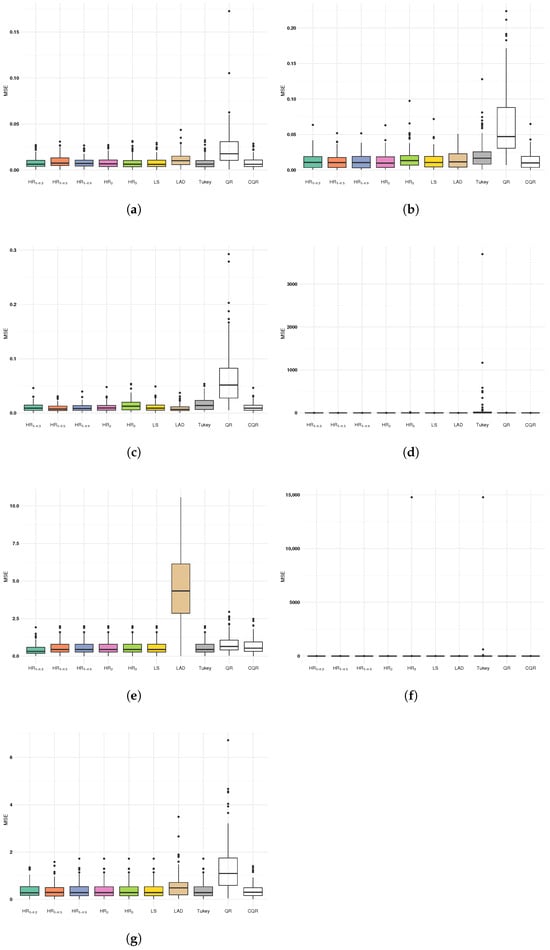
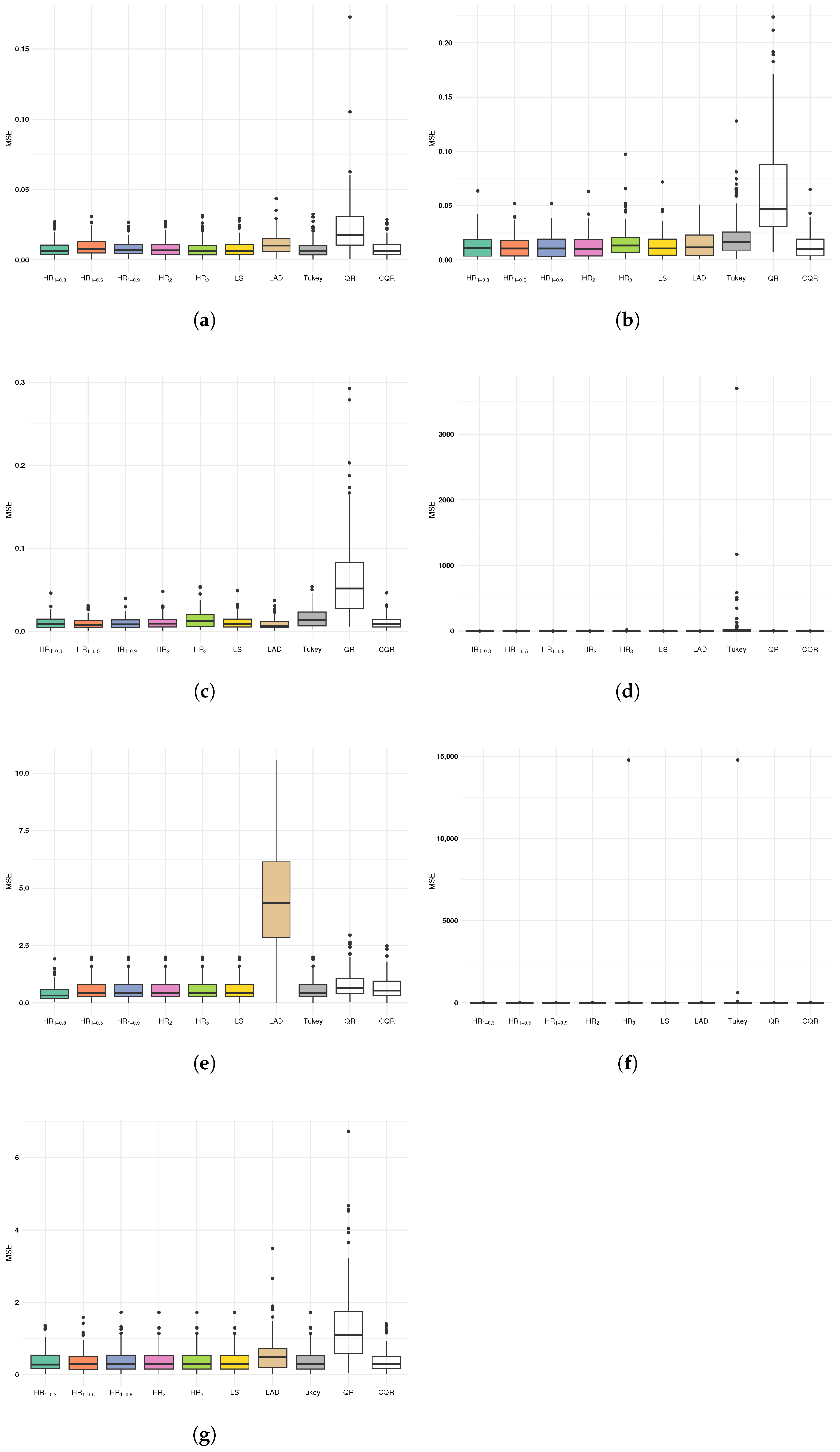
In this section, we first present simulation results to verify the lower bounds of ARE established in Theorems 1 and 2. We then present the mean squared estimation error (MSE) of the Huber estimator with the proposed choices of tuning parameters, along with the MSE of various other robust methods. Specifically, let HR₁$\left(\alpha \right)$ denotes the Huber estimator with $k=q_{\alpha }\left(\right|ϵ\left|\right)$ as described in Section 3.1. For demonstration, the parameter $\alpha$ is taken as $0.3,0.5,0.7$. Let HR₂ denote the method with k chosen as described in Section 3.2. Let HR₃ denote the Huber estimator with the rule of thumb choice for tuning parameter, $k=1.345{\displaystyle \frac{\mathrm{MAD}}{0.6745}}$. We also consider the least square (LS) estimator, least absolute deviation (LAD) estimator [6], Tukey’s bisquare (Tukey) estimator [5], quantile estimator (QR) at $\tau =0.9$ [6], and the composite quantile estimator (CQR) based on the quantile set $\tau =\{1/20,\dots ,19/20\}$ in [7].

We consider the following simulation settings:

$$\begin{array}{c}\hfill y_i=5+{\mathbf{x}}_i^{\mathrm{T}}{\beta }^{*}+{ϵ}_i,i=1,\dots ,n,\end{array}$$

(15)

where ${\mathbf{x}}_i,{\beta }^{*}\in {\mathbb{R}}^p$. The predictor $\mathbf{x}$ was generated from a multivariate normal distribution with mean $\mathbf{0}$ and covariance matrix ${\Sigma }_x$ with ${\Sigma }_x={(0.8^{|k-\ell |})}_{k,\ell =1}^p$. Besides, all elements in ${\beta }^{*}$ are 1. A wide range of commonly used error distributions were considered:

(I)

The standard normal distribution $N(0,1)$;

(II)

Student’s t-distribution with 3 degrees of freedom $t_3$;

(III)

The standard Laplace distribution $Laplace$$(0,1)$;

(IV)

The standard Cauchy distribution $Cauchy(0,1)$;

(V)

A symmetric Gamma distribution $sGamma(4,2)$, which is the distribution of a random variable $ZV$ where Z equals 1 and $-1$ each with probability $\frac{1}{2}$, V is independent of Z and follows $Gamma(4,2)$ with shape parameter 4 and scale parameter 2;

(VI)

A mixture distribution $0.9N(0,1)+0.1Cauchy(0,1)$;

(VII)

A Gamma distribution $Gamma(10,2)$, with shape parameter 10 and scale parameter 2.

The distributions in (I)–(V) are symmetric and heavy-tailed to different extents, while the distribution in (V) is bimodal. The distribution in (VI) is a setting where a portion of data is severely contaminated by outliers, and the distribution in (VII) is asymmetric. We set $n=250,500$ and $p=5,10,20,50$. All the simulation results are obtained based on 100 replications. To save space, the results corresponding to $n=250$ are placed in Appendix A.

Table 1, Table 2, Table 3, Table 4 and Table 5 present our simulation results. We use “$Mix$” in these tables to denote the distribution in (VI). Table 1 compares the empirical ARE obtained by the ratio of MSE with the theoretical lower bound (T.L.B.) of ARE established in Theorems 1 and 2, for the Huber estimators HR₁$(\alpha =0.3)$, HR₁$(\alpha =0.5)$, HR₁$(\alpha =0.7)$ and HR₂. It can be seen that the empirical ARE is indeed larger than the T.L.B across different error distributions, which confirms the correctness of our theory. Table 2, Table 3, Table 4 and Table 5 present the MSE (with standard errors in parentheses) by varying $p=5,10,20$ and 50, with the best-performing method highlighted in bold. For graphical illustration, we also provide the corresponding boxplots of the MSE for all the considered estimators in Figure 1. We reach a unified conclusion across all different choices of dimensions. Under the normal distribution, the LS estimator performs well, and most robust estimators HR₁, HR₂, HR₃, Tukey, CQR achieve comparable or slightly larger MSE. LAD and QR perform worse than other robust methods, which is not surprising given that the worst-case ARE of these methods equals zero. Under heavy-tailed distributions such as $t_3$, $Laplace(0,1)$, and $Cauchy(0,1)$, the LS estimator deteriorates sharply, especially under $Cauchy(0,1)$, where its MSE reaches 8129.35 for $p=5$ and even worse for larger p. In contrast, HR₁ estimators (particularly with $\alpha =0.3$) maintain much lower MSE, demonstrating strong robustness. HR₂ and QR also perform poorly under $Cauchy(0,1)$, while LAD and Tukey remain relatively stable. Under the symmetric Gamma distribution, $sGamma(4,2)$, all methods except LAD and QR yield similar MSE, while LAD and QR exhibit much higher MSE. Under the contaminated Mix distribution, LS and HR₂ break down completely, with extremely large MSE values. HR₁ (especially $\alpha =0.7$) and Tukey perform best, maintaining low MSE. Under the asymmetric $Gamma(10,2)$ distribution, LS and most robust methods produce similar MSE around 38.68, while LAD and QR show notably higher MSE. Overall, these results demonstrate that the Huber estimator with the proposed tuning strategies delivers acceptable performance compared with other robust methods. Across all scenarios, we see robust performance of the proposed method, while the performances of other methods may deteriorate in certain cases.

Table 1. Comparison of empirical ARE and theoretical lower bound (T.L.B.) when $n=500$.

Method	N(0, 1)	${\mathit{t}}_3$	$\mathit{Laplace}$	$\mathit{Cauchy}$ (0, 1)	$\mathit{sGamma}$ (4, 2)	$\mathit{Mix}$	$\mathit{Gamma}$ (10, 2)	T.L.B.
$p=5$
HR1 ($\alpha =0.3$)	1.083	3.460	2.480	3448.13	1.000	13,091.37	1.093	0.090
HR1 ($\alpha =0.5$)	1.070	3.120	2.079	2794.17	1.000	14,234.17	1.008	0.250
HR1 ($\alpha =0.7$)	1.016	2.658	1.865	2106.47	1.000	14,370.35	1.000	0.490
HR2	1.007	1.492	1.157	99.31	1.000	136.13	1.000	0.113
$p=10$
HR1 ($\alpha =0.3$)	0.860	2.558	1.986	26,123.48	1.000	345.47	1.044	0.045
HR1 ($\alpha =0.5$)	0.907	2.551	1.786	22,103.34	1.000	358.24	1.006	0.125
HR1 ($\alpha =0.7$)	0.949	2.264	1.522	9947.86	1.000	376.96	1.000	0.245
HR2	1.001	1.517	1.093	51.31	1.000	122.11	1.000	0.113
$p=20$
HR1 ($\alpha =0.3$)	0.769	2.075	1.710	163,51.09	1.000	44.35	1.046	0.090
HR1 ($\alpha =0.5$)	0.823	2.171	1.613	14,498.26	1.000	48.30	1.002	0.250
HR1 ($\alpha =0.7$)	0.890	2.068	1.447	10,167.50	1.000	51.24	1.000	0.490
HR2	0.998	1.469	1.069	43.00	1.000	33.65	1.000	0.113
$p=50$
HR1 ($\alpha =0.3$)	0.748	1.829	1.451	21,478.13	1.000	7908.33	1.025	0.090
HR1 ($\alpha =0.5$)	0.813	1.962	1.465	14,742.17	1.000	9342.46	1.003	0.250
HR1 ($\alpha =0.7$)	0.898	1.930	1.365	9381.29	1.000	10,638.49	1.000	0.490
HR2	1.000	1.453	1.063	11.68	1.000	92.36	1.000	0.113

Note: The maximum empirical ARE among all methods is indicated in bold face.

Table 2. Comparison of estimation MSE ($\times {10}^{-2}$) and corresponding standard errors ($\times {10}^{-2}$ in parentheses) for simulation models with $(n,p)=(500,5)$.

Method	N(0, 1)	${\mathit{t}}_3$	$\mathit{Laplace}$	$\mathit{Cauchy}$ (0, 1)	$\mathit{sGamma}$ (4, 2)	$\mathit{Mix}$	$\mathit{Gamma}$ (10, 2)
HR1 ($\alpha =0.3$)	0.955	1.239	0.925	1.806	58.814	1.135	37.480
	(0.065)	(0.105)	(0.068)	(0.139)	(4.444)	(0.080)	(3.031)
HR1 ($\alpha =0.5$)	0.864	1.211	0.985	2.236	58.814	0.990	38.598
	(0.059)	(0.104)	(0.071)	(0.166)	(4.444)	(0.066)	(3.121)
HR1 ($\alpha =0.7$)	0.823	1.264	1.069	3.603	58.814	0.899	38.674
	(0.059)	(0.110)	(0.079)	(0.279)	(4.444)	(0.062)	(3.119)
HR2	0.801	1.705	1.467	71.194	58.814	14,774.76	38.680
	(0.063)	(0.152)	(0.109)	(21.070)	(4.444)	(14,773.6)	(3.119)
HR3	0.810	1.325	1.113	3.600	58.814	0.852	38.680
	(0.060)	(0.117)	(0.081)	(0.271)	(4.444)	(0.061)	(3.119)
LS	0.805	2.218	1.624	8129.35	58.814	15,594.94	38.680
	(0.064)	(0.210)	(0.117)	(3946.8)	(4.444)	(14,778.4)	(3.119)
LAD	1.150	1.425	0.903	1.753	460.852	1.392	58.903
	(0.078)	(0.115)	(0.072)	(0.135)	(25.204)	(0.104)	(5.549)
Tukey	0.796	1.266	1.100	2.136	68.296	0.816	37.712
	(0.060)	(0.114)	(0.080)	(0.153)	(5.139)	(0.056)	(3.065)
QR	2.372	6.599	6.729	67.661	83.126	2.494	139.111
	(0.224)	(0.513)	(0.550)	(5.436)	(6.373)	(0.162)	(11.804)
CQR	0.796	1.286	1.061	2.458	43.676	0.854	37.893
	(0.059)	(0.111)	(0.078)	(0.177)	(3.520)	(0.060)	(3.138)

Note: The minimum MSE among all methods is indicated in bold face.

Table 3. Comparison of estimation MSE ($\times {10}^{-2}$) and corresponding standard errors ($\times {10}^{-2}$ in parentheses) for simulation models with $(n,p)=(500,10)$.

Method	N(0, 1)	${\mathit{t}}_3$	$\mathit{Laplace}$	$\mathit{Cauchy}$ (0, 1)	$\mathit{sGamma}$ (4, 2)	$\mathit{Mix}$	$\mathit{Gamma}$ (10, 2)
HR1 ($\alpha =0.3$)	1.113	1.339	1.045	2.191	62.849	1.283	31.567
	(0.055)	(0.066)	(0.064)	(0.115)	(3.125)	(0.075)	(1.718)
HR1 ($\alpha =0.5$)	0.995	1.277	1.127	2.796	62.849	1.174	32.585
	(0.050)	(0.064)	(0.069)	(0.161)	(3.125)	(0.071)	(1.751)
HR1 ($\alpha =0.7$)	0.902	1.337	1.272	4.417	62.849	1.066	32.723
	(0.044)	(0.067)	(0.074)	(0.272)	(3.125)	(0.062)	(1.751)
HR2	0.825	1.828	1.631	25,653.51	62.849	1.361	32.723
	(0.041)	(0.108)	(0.086)	(19,617.4)	(3.125)	(0.093)	(1.751)
HR3	0.859	1.383	1.322	4.466	62.849	1.030	32.723
	(0.041)	(0.071)	(0.076)	(0.274)	(3.125)	(0.057)	(1.751)
LS	0.825	2.563	1.749	34,083.18	62.849	277.488	32.723
	(0.041)	(0.175)	(0.088)	(19,988.7)	(3.125)	(103.86)	(1.751)
LAD	1.330	1.537	1.123	2.301	360.833	1.443	46.731
	(0.069)	(0.073)	(0.066)	(0.132)	(14.747)	(0.085)	(2.504)
Tukey	0.860	1.393	1.322	2.604	71.739	0.999	31.674
	(0.041)	(0.074)	(0.077)	(0.148)	(3.695)	(0.058)	(1.727)
QR	2.363	6.734	7.528	68.109	99.183	3.202	158.389
	(0.124)	(0.400)	(0.372)	(4.213)	(4.842)	(0.180)	(9.249)
CQR	0.862	1.342	1.238	3.078	47.511	1.052	31.434
	(0.042)	(0.069)	(0.072)	(0.161)	(2.606)	(0.059)	(1.691)

Note: The minimum MSE among all methods is indicated in bold face.

Table 4. Comparison of estimation MSE ($\times {10}^{-2}$) and corresponding standard errors ($\times {10}^{-2}$ in parentheses) for simulation models with $(n,p)=(500,20)$.

Method	N(0, 1)	${\mathit{t}}_3$	$\mathit{Laplace}$	$\mathit{Cauchy}$ (0, 1)	$\mathit{sGamma}$ (4, 2)	$\mathit{Mix}$	$\mathit{Gamma}$ (10, 2)
HR1 ($\alpha =0.3$)	1.303	1.420	1.148	2.529	72.061	1.329	36.509
	(0.050)	(0.050)	(0.045)	(0.107)	(2.931)	(0.058)	(1.314)
HR1 ($\alpha =0.5$)	1.196	1.358	1.191	3.109	72.061	1.216	37.962
	(0.046)	(0.051)	(0.046)	(0.132)	(2.931)	(0.053)	(1.363)
HR1 ($\alpha =0.7$)	1.085	1.404	1.312	4.922	72.061	1.139	38.057
	(0.041)	(0.056)	(0.050)	(0.219)	(2.931)	(0.049)	(1.372)
HR2	0.946	1.978	1.736	35,803.35	72.061	1.330	38.057
	(0.032)	(0.083)	(0.067)	(23,704.0)	(2.931)	(0.067)	(1.372)
HR3	1.033	1.455	1.351	5.004	72.061	1.112	38.057
	(0.038)	(0.059)	(0.051)	(0.224)	(2.931)	(0.049)	(1.372)
LS	0.945	2.829	1.851	43,671.25	72.061	46.230	38.057
	(0.033)	(0.153)	(0.073)	(23,700.3)	(2.931)	(11.117)	(1.372)
LAD	1.503	1.631	1.224	2.604	303.140	1.539	56.350
	(0.058)	(0.061)	(0.049)	(0.104)	(8.671)	(0.067)	(2.194)
Tukey	1.023	1.412	1.356	2.908	82.182	1.094	37.253
	(0.038)	(0.053)	(0.052)	(0.111)	(3.357)	(0.048)	(1.372)
QR	2.480	7.613	7.066	65.740	99.466	3.682	162.589
	(0.100)	(0.326)	(0.296)	(3.259)	(4.106)	(0.175)	(5.643)
CQR	1.024	1.428	1.307	3.456	59.595	1.121	37.277
	(0.038)	(0.057)	(0.050)	(0.147)	(2.739)	(0.049)	(1.378)

Note: The minimum MSE among all methods is indicated in bold face.

Table 5. Comparison of estimation MSE ($\times {10}^{-2}$) and corresponding standard errors ($\times {10}^{-2}$ in parentheses) for simulation models with $(n,p)=(500,50)$.

Method	N(0, 1)	${\mathit{t}}_3$	$\mathit{Laplace}$	$\mathit{Cauchy}$ (0, 1)	$\mathit{sGamma}$ (4, 2)	$\mathit{Mix}$	$\mathit{Gamma}$ (10, 2)
HR1 ($\alpha =0.3$)	1.365	1.759	1.442	3.022	84.065	1.542	40.510
	(0.036)	(0.046)	(0.043)	(0.106)	(1.849)	(0.042)	(0.935)
HR1 ($\alpha =0.5$)	1.244	1.644	1.415	3.539	84.076	1.402	41.404
	(0.032)	(0.042)	(0.041)	(0.128)	(1.851)	(0.037)	(1.024)
HR1 ($\alpha =0.7$)	1.120	1.654	1.499	5.614	84.076	1.272	41.530
	(0.029)	(0.043)	(0.042)	(0.202)	(1.851)	(0.033)	(1.028)
HR2	0.998	2.150	1.906	38,743.42	84.076	23,533.04	41.529
	(0.026)	(0.059)	(0.054)	(25,373.1)	(1.851)	(23,531.5)	(1.029)
HR3	1.079	1.679	1.531	5.624	84.076	1.238	41.529
	(0.028)	(0.044)	(0.042)	(0.205)	(1.851)	(0.031)	(1.029)
LS	0.998	3.068	2.020	41,371.52	84.076	23,745.08	41.529
	(0.026)	(0.167)	(0.056)	(25,345.2)	(1.851)	(23,529.4)	(1.029)
LAD	1.530	1.977	1.603	3.296	236.177	1.741	60.313
	(0.042)	(0.049)	(0.046)	(0.118)	(4.096)	(0.047)	(1.296)
Tukey	1.063	1.691	1.617	3.249	95.169	1.203	41.539
	(0.028)	(0.048)	(0.043)	(0.112)	(2.131)	(0.032)	(0.962)
QR	2.853	7.955	7.282	67.656	124.341	3.944	174.686
	(0.071)	(0.260)	(0.222)	(2.841)	(3.551)	(0.109)	(4.551)
CQR	1.055	1.661	1.505	91.122	84.795	2.775	40.620
	(0.028)	(0.044)	(0.043)	(87.019)	(2.222)	(1.548)	(0.957)

Note: The minimum MSE among all methods is indicated in bold face.

Figure 1. Boxplots for MSE across different error distributions when $(n,p)=(500,5)$. (a) $N(0,1)$. (b) $t_3$. (c) $Laplace(0,1)$. (d) $Cauchy(0,1)$. (e) $sGamma(4,2)$. (f) $Mix$. (g) $Gamma(10,2)$.

6. Conclusions

Our theoretical analysis formally establishes that Huber regression enjoys a strictly positive lower bound for its asymptotic relative efficiency compared to ordinary least squares. We give two types of choices of the robustification parameter k and establish the lower bound for each case, with the first being valid for arbitrary continuous and symmetric error distributions and the second being valid for any continuous and symmetric error with a finite first moment. We further prove that the efficiency of Huber regression is not affected by the estimation of the nuisance tuning parameter, under mild conditions. These mathematical guarantees strengthen the rationale for employing Huber regression as a safe and flexible methodology in modern statistical practice.

References

- Huber, P.J. Robust Estimation of A Location Parameter. Ann. Math. Stat. 1964, 35, 73–101. [Google Scholar] [CrossRef] [Scilit]
- Huber, P.J. Robust Statistics; John Wiley & Sons: Hoboken, NJ, USA, 2004; Volume 523. [Google Scholar]
- Fan, J.; Wang, W.; Zhu, Z. A shrinkage principle for heavy-tailed data: High-dimensional robust low-rank matrix recovery. Ann. Stat. 2021, 49, 1239. [Google Scholar] [CrossRef] [Scilit] [PubMed]
- Jaeckel, L.A. Estimating regression coefficients by minimizing the dispersion of the residuals. Ann. Math. Stat. 1972, 43, 1449–1458. [Google Scholar] [CrossRef] [Scilit]
- Beaton, A.E.; Tukey, J.W. The Fitting of Power Series, Meaning Polynomials, Illustrated on Band-Spectroscopic Data. Technometrics 1974, 16, 147–185. [Google Scholar] [CrossRef]
- Koenker, R. Quantile regression. In Econometric Society Monographs; Cambridge University Press: Cambridge, UK, 2005. [Google Scholar]
- Zou, H.; Yuan, M. Composite quantile regression and the oracle model selection theory. Ann. Stat. 2008, 36, 1108–1126. [Google Scholar] [CrossRef] [Scilit]
- Hampel, F.R. Robust statistics: A brief introduction and overview. In Seminar für Statistik; ETH Zürich: Zürich, Switzerland, 2001. [Google Scholar]
- Sun, Q.; Zhou, W.X.; Fan, J. Adaptive huber regression. J. Am. Stat. Assoc. 2020, 115, 254–265. [Google Scholar] [CrossRef] [Scilit] [PubMed]
- Wang, L.; Zheng, C.; Zhou, W.; Zhou, W.X. A new principle for tuning-free Huber regression. J. Am. Stat. Assoc. 2021, 115, 254–265. [Google Scholar] [CrossRef] [Scilit]
- Zhou, L.; Cook, R.D.; Zou, H. Enveloped huber regression. J. Am. Stat. Assoc. 2024, 119, 2722–2732. [Google Scholar] [CrossRef] [Scilit]
- Wang, Y.; Wang, B.; Peng, C.; Li, X.; Yin, H. Huber regression analysis with a semi-supervised method. Mathematics 2022, 10, 3734. [Google Scholar] [CrossRef] [Scilit]
- Tsakonas, E.; Jaldén, J.; Sidiropoulos, N.D. Convergence of the huber regression m-estimate in the presence of dense outliers. IEEE Signal Process. Lett. 2014, 21, 1211–1214. [Google Scholar] [CrossRef] [Scilit]
- Hettmansperger, T.P.; McKean, J.W. Robust Nonparametric Statistical Methods, 2nd ed.; CRC Press: Boca Raton, FL, USA, 2010. [Google Scholar]
- Hodges, J.L., Jr.; Lehmann, E.L. The efficiency of some nonparametric competitors of the t-test. Ann. Math. Stat. 1956, 27, 324–335. [Google Scholar] [CrossRef] [Scilit]
- Gu, Y.; Zou, H. Sparse composite quantile regression in ultrahigh dimensions with tuning parameter calibration. IEEE Trans. Inf. Theory 2020, 66, 7132–7154. [Google Scholar] [CrossRef] [Scilit]
- Ronchetti, E.M.; Huber, P.J. Robust Statistics, 2nd ed.; John Wiley & Sons: Hoboken, NJ, USA, 2009. [Google Scholar]
- Van der Vaart, A.W. Asymptotic Statistics; Cambridge University Press: Cambridge, UK, 2000; Volume 3. [Google Scholar]
- Van der Vaart, A.W.; Wellner, J.A. Weak Convergence and Empirical Processes: With Applications to Statistics; Springer: Cham, Switzerland, 2023. [Google Scholar]
Disclaimer/Publisher’s Note: The statements, opinions and data contained in all publications are solely those of the individual author(s) and contributor(s) and not of MDPI and/or the editor(s). MDPI and/or the editor(s) disclaim responsibility for any injury to people or property resulting from any ideas, methods, instructions or products referred to in the content. |
© 2026 by the authors. Licensee MDPI, Basel, Switzerland. This article is an open access article distributed under the terms and conditions of the Creative Commons Attribution (CC BY) license.