The Legendre Spectral Method for Solving the Nonlinear Time-Fractional Convection-Diffusion Equations

Abstract

In this paper, the nonlinear time-fractional convection-diffusion equations are solved by the Legendre spectral method. The Caputo time-fractional derivative is discretized by the $L2$–$1_{\sigma }$ scheme. A priori estimates of the fully discrete scheme are derived, and the existence and uniqueness of the numerical solution are analyzed. It is rigorously proved that the fully discrete scheme is unconditionally stable, and the convergence order of the numerical scheme is $O(N^{1-m}+{\tau }^2)$. Finally, numerical results are presented to verify the theoretical analysis.

1. Introduction

In recent years, with the applications of fractional derivatives in various fields [1,2,3,4,5,6], nonlinear fractional convection-diffusion equations have garnered growing attention. Computational simulations, including reservoir simulation, substance and energy transport, and global climate generation, are often carried out with the utilization of such equations [7].

Numerical methods for solving fractional partial differential equations mainly include finite difference methods [8,9,10,11], finite element methods [12,13,14,15,16], finite volume methods [17,18,19,20], spectral methods [21,22,23,24], etc.

In this paper, we consider the following nonlinear time-fractional convection-diffusion equation [25]:

$$\left\{\begin{array}{cc}{}_0{}^{C}D_t^{\alpha }u(x,t)-\mu {\mathsf{\partial }}_x^{2}u(x,t)+{\mathsf{\partial }}_{x}u(x,t)+g\left(u(x,t)\right)=f(x,t),\hfill & (x,t)\in \Lambda \times (0,T],\hfill \\ u(-1,t)=0,u(1,t)=0,\hfill & t\in [0,T],\hfill \\ u(x,0)=u_0\left(x\right),\hfill & x\in \Lambda ,\hfill \end{array}\right.$$

(1)

where $0<\alpha <1$, $\Lambda =(-1,1)$, and $\mu >0$. The nonlinear term $g\left(u\right)$ satisfies $g^{\prime }\left(u\right)>{\displaystyle \frac{1+\mu }{4\mu }}$, and $g^{\prime }\left(u\right)$ is bounded. Without loss of generality, we assume $g\left(0\right)=0$ throughout the work. ${}_0{}^{C}D_t^{\alpha }u(x,t)$ represents the Caputo time-fractional derivative, defined as

$${}_0{}^{C}D_t^{\alpha }u(x,t)={\displaystyle \frac{1}{\Gamma (1-\alpha )}}{\int }_0^t{\displaystyle \frac{\mathsf{\partial }u(x,\tau )}{\mathsf{\partial }\tau }}{\displaystyle \frac{d\tau }{{(t-\tau )}^{\alpha }}},0<\alpha <1$$

where $\Gamma (·)$ is the gamma function.

Priyanka and Sahani et al. [26] used the $L1$ scheme and the Hermite collocation method in time and space, respectively, to solve the two-dimensional time-fractional sub-diffusion equation. This method had $2-\alpha$ order convergence in time and fourth-order convergence in space. Mohammadi et al. [27] constructed a fully discrete scheme based upon the fourth-order exponential time-differencing Runge–Kutta method and Fourier spectral method, where the convergence order was $O(N^{\mu -m}+{\tau }^{3-\alpha })$. Londoño et al. [28] proposed an effective numerical method for the two-dimensional time-fractional advection–dispersion equation, using the $L1$–2–3 scheme and Radial basis function (RBF) method in time and space, respectively. Singh and Kumar [29] applied $L2$–$1_{\sigma }$ with nonuniform time mesh for the time-fractional derivative. The spatial direction was discretized using the high-order compact alternating-direction implicit (ADI) scheme, with convergence orders of $O\left(N_t^{-min\{3-\alpha ,\theta ,\alpha ,1+2\alpha ,2+\alpha \}}+h_x^4+h_y^4\right)$. In [30], two numerical schemes were proposed for solving convection-diffusion delay differential equations. The first scheme employs the $L1$–2 scheme to the discrete Caputo fractional derivative and triangular spline technique to discretize the spatial variable. This method had $3-\alpha$ convergence in time and second-order convergence in space, respectively. The second scheme combines the novel MABC operator with the triangular spline method and achieves second-order accuracy in both temporal and spatial directions. Both schemes are unconditionally stable and convergent.

In this paper, a nonlinear fully discrete scheme is constructed for the nonlinear time-fractional convection-diffusion equation. The $L2$–$1_{\sigma }$ scheme is utilized for time discretization, while the Legendre spectral method is applied for spatial approximation. Compared to the Chebyshev/Jacobi methods, the Legendre spectral method offers better numerical stability by avoiding endpoint singularity-induced oscillations and using a diagonal mass matrix for higher efficiency. A priori error estimates of the numerical solution for the fully discrete scheme are presented. The existence and uniqueness of the solution to the fully discrete scheme are proved using the Brouwer fixed-point theorem. This work provides a rigorous error analysis for the nonlinear case, a key contribution that distinguishes it from existing linear-focused studies. It is demonstrated that this scheme is unconditionally stable and the convergence rate is of the order $O(N^{1-m}+{\tau }^2)$.

The rest of this paper is organized as follows: Some preliminaries and notations will be introduced in the next section. In Section 3, we construct a fully discrete scheme, where the $L2$–$1_{\sigma }$ scheme is applied for temporal discretization and the Legendre spectral method is used for spatial discretization, and a priori estimates are provided. In Section 4, the existence and uniqueness of solutions for the fully discrete scheme are analyzed. We prove the unconditional stability and convergence of the fully discrete scheme in Section 5. In Section 6, numerical examples are provided to verify the theoretical results. The conclusion is presented in Section 7.

2. Preliminaries and Notations

Denote $\Lambda =(-1,1)$. The inner product of $L^2(\Lambda )$ is denoted by $(·,·)$. Let $L^2(\Lambda )$, $L^{\infty }(\Lambda )$, and $H^m(\Lambda )=\{u:u\in L^2(\Lambda ),{\mathsf{\partial }}^{i}u\in L^2(\Lambda ),0\le i\le m\}$ be the usual Sobolev spaces equipped with norms $\parallel ·\parallel$, ${\parallel ·\parallel }_{\infty }$ and ${\parallel ·\parallel }_m$, respectively. $H_0^1(\Lambda )=\{u:u\in H^1(\Lambda ),u(\pm 1)=0\}$.

Define the space-time Sobolev space $L^{\infty }(0,T;H^m(\Lambda )):(0,T)\to H^m(\Lambda )$, endowed with the norm

$${\parallel u\parallel }_{L^{\infty }\left(H^m(\Lambda )\right)}=\underset{0\le t\le T}{\mathrm{ess}\sup }{\parallel u\left(t\right)\parallel }_m.$$

The definitions of other space-time Sobolev spaces are similar to those given above. Throughout this paper, c denotes a generic positive constant.

Let N be a non-negative integer and ${\varphi }_i\left(x\right)=L_i\left(x\right)-L_{i+2}\left(x\right)$, $i=0,1,\cdots ,N-2$ be the basis functions [31], where $L_i\left(x\right)$ is an i-degree Legendre polynomial. The basis function space is $S_N=\mathrm{span}\{{\varphi }_i\left(x\right),i=0,1,\cdots ,N-2\}$.

Let ${\Pi }_N^{1,0}:H_0^1(\Lambda )\to S_N$ represent the orthogonal projection operator and satisfy

$$({(u-{\Pi }_N^{1,0}u)}^{\prime },{\varphi }^{\prime })=0,\forall \varphi \in S_N.$$

For convenience, we denote ${\mathsf{\partial }}_x^{k}u\left(x\right)={\displaystyle \frac{d^k}{d{x}^k}}u\left(x\right)$. For this projection operator, we have the following approximation results.

Lemma 1 

([32]). Assume $u\in H^m(\Lambda )\cap H_0^1(\Lambda )$; then

$$\parallel u-{\Pi }_N^{1,0}{u\parallel }_s\le c{N}^{s-m}{\parallel u\parallel }_m,s=0,1,$$

where c is independent of N and u.

3. The Fully Discrete Scheme

In this section, we construct the fully discrete scheme for the equation. The time step is $\tau ={\displaystyle \frac{T}{M}}$, $t_k=k\tau$, $u^k=u(x,t_k)$, $k=0,1,...,M$. Let $t_{k+\sigma }=(k+\sigma )\tau$, $\sigma =1-{\displaystyle \frac{\alpha }{2}}$, $u^k=u(x,t_k)$ and $u^{k+\sigma }=u(x,t_{k+\sigma })$. We also denote $u^{k,\sigma }=\sigma u^{k+1}+(1-\sigma )u^k$. The discretization of the Caputo time-fractional derivative using the $L2$–$1_{\sigma }$ scheme is defined as [33]

$$A_{\tau }^{\alpha }{u}^{k+\sigma }=\sum _{j=0}^k{a}_j^{k+1}(u^{j+1}-u^j),$$

where $a_j^{k+1}={\displaystyle \frac{{\tau }^{-\alpha }{c}_{k-j}}{\Gamma (2-\alpha )}}$, $k\ge 1$,

$$c_j=\left\{\begin{array}{cc}{d}_0+b_1,\hfill & j=0,\hfill \\ d_j+b_{j+1}-b_j,\hfill & 1\le j\le k-1,\hfill \\ d_k+b_k,\hfill & j=k.\hfill \end{array}\right.$$

$$d_0={\sigma }^{1-\alpha },d_j={(j+\sigma )}^{1-\alpha }-{(j+\sigma -1)}^{1-\alpha },j\ge 1,$$

$$b_j={\displaystyle \frac{1}{2-\alpha }}[{(j+\sigma )}^{2-\alpha }-{(j+\sigma -1)}^{2-\alpha }]-{\displaystyle \frac{1}{2}}[{(j+\sigma )}^{1-\alpha }+{(j+\sigma -1)}^{1-\alpha }].$$

The $L2$–$1_{\sigma }$ scheme’s coefficient ${\left\{c_j\right\}}_{j=0}^k$ (with $k\ge 1$) and truncation error have the following properties.

Lemma 2 

([34]). For any coefficient ${\left\{c_j\right\}}_{j=0}^k$, $k\ge 1$ and any $0<\alpha <1$, it holds that

$${\displaystyle \frac{1-\alpha }{2{(k+\sigma )}^{\alpha }}}<c_k,{\displaystyle \frac{\sigma }{2\sigma -1}}{c}_1<c_0,c_k<c_{k-1}<\cdots <c_1<c_0.$$

Lemma 3 

([34]). For any $0<\alpha <1$ and $u\left(t\right)\in C^3[0,t_{k+1}]$, the following inequality holds:

$$|{}_0{}^{C}D_t^{\alpha }{u}^{k+\sigma }-A_{\tau }^{\alpha }{u}^{k+\sigma }|\le c{\tau }^{3-\alpha }.$$

Lemma 4 

([33]). For any $u\in S_N^0$, we have

$$\left(u^{k,\sigma },A_{\tau }^{\alpha }{u}^{k+\sigma }\right)\ge {\displaystyle \frac{1}{2}}{A}_{\tau }^{\alpha }{\parallel u^{k+\sigma }\parallel }^2,0\le k\le M-1.$$

For spatial discretization, we use the Legendre spectral method and $g\left(u^{k,\sigma }\right)$ to approximate the nonlinear term $g\left(u^{k+\sigma }\right)$. The fully discrete scheme of Equation (1) is as follows: find $u_N^{k+1}\in S_N$, for $\forall \phi \in S_N$, such that

$$\left\{\begin{array}{c}(A_{\tau }^{\alpha }{u}_N^{k+\sigma },\phi )+\mu ({\mathsf{\partial }}_x{u}_N^{k,\sigma },{\mathsf{\partial }}_x\phi )+({\mathsf{\partial }}_x{u}_N^{k,\sigma },\phi )+(g\left(u_N^{k,\sigma }\right),\phi )=(f^{k+\sigma },\phi ),\hfill \\ u_0={\Pi }_N^{1,0}{u}_0.\hfill \end{array}\right.$$

(2)

Next, we present a priori estimates.

Lemma 5. 

For the solution $u_N^{k+1}\in S_N$ of Equation (2), the following inequality holds:

$$\begin{array}{c}\hfill {\parallel u_N^{k+1}\parallel }^2\le \parallel u_N^0{\parallel }^2+4\Gamma (1-\alpha )T^{\alpha }\underset{0\le k\le M-1}{max}{\parallel f^{k+\sigma }\parallel }^2,0\le k\le M-1.\end{array}$$

(3)

Proof. 

Taking $\phi =u_N^{k,\sigma }$ in (2), it holds that

$$\left(A_{\tau }^{\alpha }{u}_N^{k+\sigma },u_N^{k,\sigma }\right)+\mu {∥{\mathsf{\partial }}_x{u}_N^{k,\sigma }∥}^2+\left({\mathsf{\partial }}_x{u}_N^{k,\sigma },u_N^{k,\sigma }\right)+\left(g\left(u_N^{k,\sigma }\right),u_N^{k,\sigma }\right)=\left(f^{k+\sigma },u_N^{k,\sigma }\right).$$

(4)

Applying Lemma 4, we derive that

$$\left(A_{\tau }^{\alpha }{u}_N^{k+\sigma },u_N^{k,\sigma }\right)\ge {\displaystyle \frac{1}{2}}{A}_{\tau }^{\alpha }{\parallel u_N^{k+\sigma }\parallel }^2.$$

(5)

For the third term on the left-hand side of Equation (4), by applying Hölder’s inequality and Young’s inequality, we infer that

$$\left({\mathsf{\partial }}_x{u}_N^{k,\sigma },u_N^{k,\sigma }\right)\le \mu {\parallel {\mathsf{\partial }}_x{u}_N^{k,\sigma }\parallel }^2+{\displaystyle \frac{1}{4\mu }}{\parallel u_N^{k,\sigma }\parallel }^2.$$

(6)

Applying the differentiation mean-value theorem to the fourth term on the left-hand side of (4), we deduce that

$$\left(g\left(u_N^{k,\sigma }\right),u_N^{k,\sigma }\right)=g^{\prime }\left({\xi }_1\right){\parallel u_N^{k,\sigma }\parallel }^2.$$

(7)

Substituting (5)–(7) into (4), and using Hölder’s inequality and Young’s inequality, we arrive at

$$\begin{array}{cc}\hfill {\displaystyle \frac{1}{2}}{A}_{\tau }^{\alpha }{\parallel u_N^{k+\sigma }\parallel }^2+\mu {\parallel {\mathsf{\partial }}_x{u}_N^{k,\sigma }\parallel }^2+g^{\prime }\left({\xi }_1\right){\parallel u_N^{k,\sigma }\parallel }^2\le & \left|-\left(\mu {\parallel {\mathsf{\partial }}_x{u}_N^{k,\sigma }\parallel }^2+{\displaystyle \frac{1}{4\mu }}{\parallel u_N^{k,\sigma }\parallel }^2\right)\right|\hfill \\ & +{\parallel f^{k+\sigma }\parallel }^2+{\displaystyle \frac{1}{4}}{\parallel u_N^{k,\sigma }\parallel }^2.\hfill \end{array}$$

(8)

By $g^{\prime }\left({\xi }_1\right)>{\displaystyle \frac{1+\mu }{4\mu }}$, we infer that

$$A_{\tau }^{\alpha }\parallel u_N^{k+\sigma }{\parallel }^2\le 2{\parallel f^{k+\sigma }\parallel }^2.$$

(9)

Applying the definition of operator $A_{\tau }^{\alpha }$ for (9), we derive that

$$a_k^{k+1}\parallel u_N^{k+1}{\parallel }^2\le \sum _{j=1}^k\left(a_j^{k+1}-a_{j-1}^{k+1}\right){\parallel u_N^j\parallel }^2+a_0^{k+1}\left(\parallel u_N^0{\parallel }^2+{\displaystyle \frac{2}{a_0^{k+1}}}{\parallel f^{k+\sigma }\parallel }^2\right).$$

(10)

By Lemma 2, we have ${\displaystyle \frac{1}{a_0^{k+1}}}\le 2\Gamma (1-\alpha )T^{\alpha }$. Then we deduce that

$$a_k^{k+1}\parallel u_N^{k+1}{\parallel }^2\le \sum _{j=1}^k\left(a_j^{k+1}-a_{j-1}^{k+1}\right){\parallel u_N^j\parallel }^2+a_0^{k+1}F,$$

(11)

where $F=\parallel u_N^0{\parallel }^2+4\Gamma (1-\alpha )T^{\alpha }{max}_{0\le k\le M-1}{\parallel f^{k+\sigma }\parallel }^2$.

Next, we use mathematical induction to prove inequlity (3).

Taking $k=0$ in (11), we find that $a_0^1{\parallel u_N^1\parallel }^2\le a_0^{1}F$; i.e., (3) is true for $k=0$. Next, assuming (3) holds for $j=1,2,\cdots ,k$, we get

$$\begin{array}{cc}\hfill a_k^{k+1}{\parallel u_N^{k+1}\parallel }^2& \le \sum _{j=1}^k\left(a_j^{k+1}-a_{j-1}^{k+1}\right){\parallel u_N^j\parallel }^2+a_0^{k+1}F\hfill \\ \hfill & \le \sum _{j=1}^k\left(a_j^{k+1}-a_{j-1}^{k+1}\right)F+a_0^{k+1}F=a_k^{k+1}F.\hfill \end{array}$$

(12)

Hence, (3) holds for $j=k+1$, where $k=0,1,\cdots ,M$. □

4. Existence and Uniqueness of Numerical Solution

The following Brouwer fixed-point theorem is crucial for proving the existence of the numerical solution.

Lemma 6 

([32]). Let W be a finite-dimensional Hilbert space with scalar product $(·,·)$ and norm $\parallel ·\parallel$, and let $Z:W\to W$ be a continuous map satisfying $\left(Z\right(\phi ),\phi )>0$ for $\parallel \phi \parallel =G>0$. Then there exists ${\phi }^{*}\in W$, $\parallel \phi \parallel \le G$, such that

$$Z\left({\phi }^{*}\right)=0.$$

Theorem 1. 

Given ${\left\{u_N^j\right\}}_{j=0}^k$, there exists $u_N^{k+1}$ satisfying scheme (2).

Proof. 

According to the definition of operator $A_{\tau }^{\alpha }$ and $u_N^{k,\sigma }=\sigma u_N^{k+1}+(1-\sigma )u_N^k$, (2) can be rewritten into the form

$$\begin{array}{cc}\hfill & {\displaystyle \frac{a_k^{k+1}}{\sigma }}\left(u_N^{k,\sigma },\phi \right)-{\displaystyle \frac{a_k^{k+1}(1-\sigma )}{\sigma }}\left(u_N^k,\phi \right)-\sum _{j=1}^k\left(a_j^{k+1}-a_{j-1}^{k+1}\right)\left(u_N^j,\phi \right)+\mu \left({\mathsf{\partial }}_x{u}_N^{k,\sigma },{\mathsf{\partial }}_x\phi \right)\hfill \\ \hfill & +\left({\mathsf{\partial }}_x{u}_N^{k,\sigma },\phi \right)+\left(g\left(u_N^{k,\sigma }\right),\phi \right)=\left(f^{k+\sigma },\phi \right).\hfill \end{array}$$

(13)

The mapping $Z:S_N^0(\Lambda )\to S_N^0(\Lambda )$ is defined as

$$\begin{array}{cc}\hfill & (Z\left(u_N^{k,\sigma }\right),\phi )\hfill \\ \hfill =& {\displaystyle \frac{a_k^{k+1}}{\sigma }}(u_N^{k,\sigma },\phi )+\mu ({\mathsf{\partial }}_x{u}_N^{k,\sigma },{\mathsf{\partial }}_x\phi )+({\mathsf{\partial }}_x{u}_N^{k,\sigma },\phi )+(g\left(u_N^{k,\sigma }\right),\phi )-{\displaystyle \frac{a_k^{k+1}(1-\sigma )}{\sigma }}(u_N^k,\phi )\hfill \\ \hfill & -\sum _{j=1}^k(a_j^{k+1}-a_{j-1}^{k+1})(u_N^j,\phi )-a_0^{k+1}(u_N^0,\phi )-(f^{k+\sigma },\phi ).\hfill \end{array}$$

(14)

Using $\phi =u_N^{k,\sigma }$ in (14), we have

$$\begin{array}{cc}\hfill & (Z\left(u_N^{k,\sigma }\right),u_N^{k,\sigma })\hfill \\ \hfill =& {\displaystyle \frac{a_k^{k+1}}{\sigma }}\parallel u_N^{k,\sigma }{\parallel }^2+\mu {\parallel {\mathsf{\partial }}_x{u}_N^{k,\sigma }\parallel }^2+\left(g\left(u_N^{k,\sigma }\right),u_N^{k,\sigma }\right)-\left(u_N^{k,\sigma },{\mathsf{\partial }}_x{u}_N^{k,\sigma }\right)-{\displaystyle \frac{a_k^{k+1}(1-\sigma )}{\sigma }}\left(u_N^k,u_N^{k,\sigma }\right)\hfill \\ \hfill & -\sum _{j=1}^k\left(a_j^{k+1}-a_{j-1}^{k+1}\right)\left(u_N^j,u_N^{k,\sigma }\right)-a_0^{k+1}\left(u_N^0,u_N^{k,\sigma }\right)-\left(f^{k+\sigma },u_N^{k,\sigma }\right).\hfill \end{array}$$

(15)

For the third term on the right-hand side of (14), by applying the differentiation mean-value theorem, we get

$$\left(g\left(u_N^{k,\sigma }\right),u_N^{k,\sigma }\right)=g^{\prime }\left({\xi }_2\right){\parallel u_N^{k,\sigma }\parallel }^2.$$

(16)

Applying Hölder’s inequality and Young’s inequality, it holds that

$$\left(u_N^{k,\sigma },{\mathsf{\partial }}_x{u}_N^{k,\sigma }\right)\le {\displaystyle \frac{1}{4\mu }}\parallel u_N^{k,\sigma }{\parallel }^2+\mu {\parallel {\mathsf{\partial }}_x{u}_N^{k,\sigma }\parallel }^2.$$

(17)

$$\begin{array}{cc}\hfill {\displaystyle \frac{a_k^{k+1}(1-\sigma )}{\sigma }}\left(u_N^k,u_N^{k,\sigma }\right)& \le {\displaystyle \frac{a_k^{k+1}}{2}}\parallel u_N^k{\parallel }^2+{\displaystyle \frac{a_k^{k+1}{(1-\sigma )}^2}{2{\sigma }^2}}{\parallel u_N^{k,\sigma }\parallel }^2\hfill \\ \hfill & \le {\displaystyle \frac{a_k^{k+1}}{2}}\parallel u_N^k{\parallel }^2+{\displaystyle \frac{a_k^{k+1}}{2}}{\parallel u_N^{k,\sigma }\parallel }^2,\hfill \end{array}$$

(18)

$$\begin{array}{cc}\hfill \sum _{j=1}^k\left(a_j^{k+1}-a_{j-1}^{k+1}\right)\left(u_N^j,u_N^{k,\sigma }\right)& \le \sum _{j=1}^k{\displaystyle \frac{\left(a_j^{k+1}-a_{j-1}^{k+1}\right)}{2}}\parallel u_N^j{\parallel }^2+{\displaystyle \frac{\left(a_k^{k+1}-a_0^{k+1}\right)}{2}}{\parallel u_N^{k,\sigma }\parallel }^2,\hfill \end{array}$$

(19)

$$a_0^{k+1}\left(u_N^0,u_N^{k,\sigma }\right)\le {\displaystyle \frac{a_0^{k+1}}{2}}\parallel u_N^0{\parallel }^2+{\displaystyle \frac{a_0^{k+1}}{2}}{\parallel u_N^{k,\sigma }\parallel }^2,$$

(20)

$$\left(f^{k+\sigma },u_N^{k,\sigma }\right)\le \parallel f^{k+\sigma }{\parallel }^2+{\displaystyle \frac{1}{4}}{\parallel u_N^{k,\sigma }\parallel }^2.$$

(21)

Substituting (16)–(21) into (15), it holds that

$$\begin{array}{cc}\hfill (Z\left(u_N^{k,\sigma }\right),u_N^{k,\sigma })\ge & \left({\displaystyle \frac{a_k^{k+1}}{\sigma }}+g^{\prime }\left({\xi }_2\right)-{\displaystyle \frac{1+\mu }{4\mu }}\right){\parallel u_N^{k,\sigma }\parallel }^2-\left({\displaystyle \frac{a_k^{k+1}}{2}}\parallel u_N^k{\parallel }^2+\sum _{j=1}^k{\displaystyle \frac{a_j^{k+1}-a_{j-1}^{k+1}}{2}}{\parallel u_N^j\parallel }^2\right.\hfill \\ \hfill & \left.+{\displaystyle \frac{a_0^{k+1}}{2}}\parallel u_N^0{\parallel }^2+a_k^{k+1}\parallel u_N^{k,\sigma }{\parallel }^2+{\parallel f^{k+\sigma }\parallel }^2\right).\hfill \end{array}$$

(22)

Using $g^{\prime }\left({\xi }_2\right)>{\displaystyle \frac{1+\mu }{4\mu }}$ and Lemma 5 yields

$$\begin{array}{cc}\hfill & {\displaystyle \frac{a_k^{k+1}}{2}}\parallel u_N^k{\parallel }^2+\sum _{j=1}^k{\displaystyle \frac{a_j^{k+1}-a_{j-1}^{k+1}}{2}}\parallel u_N^j{\parallel }^2+{\displaystyle \frac{a_0^{k+1}}{2}}{\parallel u_N^0\parallel }^2\hfill \\ \hfill & \le a_k^{k+1}\underset{0\le j\le k}{max}{\parallel u_N^j\parallel }^2\hfill \\ \hfill & \le a_k^{k+1}(\parallel u_N^0{\parallel }^2+4\Gamma (1-\alpha )T^{\alpha }\underset{0\le k\le M-1}{max}\parallel f^{k+\sigma }{\parallel }^2).\hfill \end{array}$$

(23)

Substituting (23) into (22), we can conclude that

$$\begin{array}{cc}\hfill (Z\left(u_N^{k,\sigma }\right),u_N^{k,\sigma })\ge & {\displaystyle \frac{a_k^{k+1}(1-\sigma )}{\sigma }}{\parallel u_N^{k,\sigma }\parallel }^2\hfill \\ \hfill & -a_k^{k+1}\left(\parallel u_N^0{\parallel }^2+4\Gamma (1-\alpha )T^{\alpha }\underset{0\le k\le M-1}{max}\parallel f^{k+\sigma }{\parallel }^2+{\displaystyle \frac{1}{a_k^{k+1}}}{\parallel f^{k+\sigma }\parallel }^2\right).\hfill \end{array}$$

(24)

Applying ${\displaystyle \frac{1}{a_k^{k+1}}}\le 2\Gamma (1-\alpha )T^{\alpha }$, we derive that

$$\begin{array}{cc}\hfill (Z\left(u_N^{k,\sigma }\right),u_N^{k,\sigma })& \ge {\displaystyle \frac{a_k^{k+1}(1-\sigma )}{\sigma }}{\parallel u_N^{k,\sigma }\parallel }^2\hfill \\ \hfill & -a_k^{k+1}(\parallel u_N^0{\parallel }^2+6\Gamma (1-\alpha )T^{\alpha }\underset{0\le k\le M-1}{max}\parallel f^{k+\sigma }{\parallel }^2).\hfill \end{array}$$

(25)

Then we have $(Z\left(u_N^{k,\sigma }\right),u_N^{k,\sigma })\ge 0$ for $\parallel u_N^{k,\sigma }\parallel =G$, where $G\ge \sqrt{{\displaystyle \frac{\sigma }{1-\sigma }}}(\parallel u_N^0{\parallel }^2+6\Gamma (1-\alpha )T^{\alpha }\underset{0\le k\le M-1}{max}\parallel f^{k+\sigma }{{\parallel }^2)}^{{\displaystyle \frac{1}{2}}}$. By Lemma 6, we know that there exists $u_N^{k,\sigma }\in S_N^0(\Lambda )$ such that $Z\left(u_N^{k,\sigma }\right)=0$. Since $u_N^{k,\sigma }=\sigma u_N^{k+1}+(1-\sigma )u_N^k$, it follows that the solution $u_N^{k+1}$ of scheme (2) exists. □

Theorem 2. 

The solution $u_N^{k+1}$ of scheme (2) is unique.

Proof. 

Suppose that ${\left\{u_N^{k+1}\right\}}_{k=0}^{M-1}$ and ${\left\{v_N^{k+1}\right\}}_{k=0}^{M-1}$ are both solutions of scheme (2) with the same initial condition. ${\Phi }_N^{k+1}=u_N^{k+1}-v_N^{k+1}$; then ${\Phi }_N^{k+1}$ satisfies the following equation:

$$(A_{\tau }^{\alpha }{\Phi }_N^{k+\sigma },\phi )+\mu ({\mathsf{\partial }}_x{\Phi }_N^{k,\sigma },{\mathsf{\partial }}_x\phi )+({\mathsf{\partial }}_x{\Phi }_N^{k,\sigma },\phi )+(g\left(u_N^{k,\sigma }\right)-g\left(v_N^{k,\sigma }\right),\phi )=0,$$

(26)

where ${\Phi }_N^0=0$. Taking $\phi ={\Phi }_N^{k,\sigma }$, and using Lemma 4, we find that

$$\begin{array}{cc}\hfill {\displaystyle \frac{1}{2}}{A}_{\tau }^{\alpha }\parallel {\Phi }_N^{k+\sigma }{\parallel }^2+\mu {\parallel {\mathsf{\partial }}_x{\Phi }_N^{k,\sigma }\parallel }^2+\left(g\left(u_N^{k,\sigma }\right)-g\left(v_N^{k,\sigma }\right),{\Phi }_N^{k,\sigma }\right)& \le \left|-({\mathsf{\partial }}_x{\Phi }_N^{k,\sigma },{\Phi }_N^{k,\sigma })\right|.\hfill \end{array}$$

(27)

By the differentiation mean-value theorem and Hölder’s inequality and Young’s inequality for (27), we can get

$$\begin{array}{cc}\hfill {\displaystyle \frac{1}{2}}{A}_{\tau }^{\alpha }\parallel {\Phi }_N^{k+\sigma }{\parallel }^2+\mu \parallel {\mathsf{\partial }}_x{\Phi }_N^{k,\sigma }{\parallel }^2+g^{\prime }\left({\xi }_3\right){\parallel {\Phi }_N^{k,\sigma }\parallel }^2& \le \mu \parallel {\mathsf{\partial }}_x{\Phi }_N^{k,\sigma }{\parallel }^2+{\displaystyle \frac{1}{4\mu }}{\parallel {\Phi }_N^{k,\sigma }\parallel }^2.\hfill \end{array}$$

(28)

Due to $g^{\prime }\left({\xi }_3\right)>{\displaystyle \frac{1+\mu }{4\mu }}$, (27) can be rewritten as

$$A_{\tau }^{\alpha }{\parallel {\Phi }_N^{k+\sigma }\parallel }^2\le 0.$$

(29)

According to the definition of operator $A_{\tau }^{\alpha }$, we can derive that

$$a_k^{k+1}\parallel {\Phi }_N^{k+1}{\parallel }^2\le \sum _{j=1}^k(a_j^{k+1}-a_{j-1}^{k+1})\parallel {\Phi }_N^j{\parallel }^2+a_0^{k+1}{\parallel {\Phi }_N^0\parallel }^2.$$

(30)

We use mathematical induction to prove the following inequality:

$$a_k^{k+1}\parallel {\Phi }_N^{k+1}{\parallel }^2\le a_0^{k+1}{\parallel {\Phi }_N^0\parallel }^2.$$

(31)

For $k=0$, substituting into (30) yields $a_0^1\parallel {\Phi }_N^1{\parallel }^2\le a_0^1{\parallel {\Phi }_N^0\parallel }^2$, so (31) holds. Assume that (31) holds for $j=1,2,\dots ,k$. Then, by (30), we have

$$a_k^{k+1}\parallel {\Phi }_N^{k+1}{\parallel }^2\le \sum _{j=1}^k(a_j^{k+1}-a_{j-1}^{k+1})\parallel {\Phi }_N^0{\parallel }^2+a_0^{k+1}\parallel {\Phi }_N^0{\parallel }^2=a_k^{k+1}{\parallel {\Phi }_N^0\parallel }^2.$$

(32)

Thus, (31) holds for all k. Since ${\Phi }_N^0=0$, we conclude that ${\Phi }_N^{k+1}=u_N^{k+1}-v_N^{k+1}=0$; hence the solution of scheme (2) is unique. □

5. Stability and Convergence Analysis

In this section, we prove the stability and convergence of the proposed numerical scheme. We analyze the stability of the numerical scheme. Let ${\left\{{\tilde{u}}_N^{k+1}\right\}}_{k=0}^{M-1}\in S_N$ be the solution of the following equation:

$$\left\{\begin{array}{c}(A_{\tau }^{\alpha }{\tilde{u}}_N^{k+\sigma },\phi )+\mu ({\mathsf{\partial }}_x{\tilde{u}}_N^{k,\sigma },{\mathsf{\partial }}_x\phi )+({\mathsf{\partial }}_x{\tilde{u}}_N^{k,\sigma },\phi )+\left(g\left({\tilde{u}}_N^{k,\sigma }\right),\phi \right)=({\tilde{f}}^{k+\sigma },\phi ),\hfill \\ {\tilde{u}}_0={\Pi }_N^{1,0}{\tilde{u}}_0.\hfill \end{array}\right.$$

(33)

We have the following conclusion.

Theorem 3. 

Let ${\left\{u_N^{k+1}\right\}}_{k=0}^{M-1}$ be the solution of Equation (2) and ${\left\{{\tilde{u}}_N^{k+1}\right\}}_{k=0}^{M-1}$ be the solution of Equation (33), $0\le k\le M-1$; then

$$\parallel u_N^{k+1}-{\tilde{u}}_N^{k+1}\parallel \le \parallel u_N^0-{\tilde{u}}_N^0\parallel +4\Gamma (1-\alpha )T^{\alpha }\underset{0\le k\le M-1}{max}\parallel f^{k+\sigma }-{\tilde{f}}^{k+\sigma }\parallel .$$

Proof. 

It is trivial to obtain the stability result by following the proofs of Lemma 5 and Theorem 2. □

Next, we provide the convergence analysis of the fully discrete schemes.

Theorem 4. 

Let ${\left\{u^k\right\}}_{k=0}^M$ be the solution of Equation (1) and ${\left\{u_N^k\right\}}_{k=0}^M$ be the solution of the fully discrete scheme (2), $0\le k\le M$. Assuming $u\in C^3(0,T)\cap L^{\infty }(0,T;H^m(\Lambda ))$ and ${}_0{}^{C}D_t^{\alpha }u\in L^{\infty }(0,T;H^m(\Lambda ))$,

$$\parallel u^k-u_N^k\parallel \le C({\tau }^2+N^{1-m}),0\le k\le M,$$

where C is a positive constant, which is independent of N and τ.

Proof. 

Denote ${\rho }^k=u^k-u_N^k=(u^k-{\Pi }_N^{1,0}{u}^k)+({\Pi }_N^{1,0}{u}^k-u_N^k)\stackrel{\Delta }{=}{\eta }^k+e_N^k$. Let $\phi =e_N^k\in S_N$. From (1) and (27), we obtain the following error equation:

$$\begin{array}{cc}\hfill & (A_{\tau }^{\alpha }{e}_N^{k+\sigma },e_N^{k,\sigma })+\mu ({\mathsf{\partial }}_x{e}_N^{k,\sigma },{\mathsf{\partial }}_x{e}_N^{k,\sigma })+\left(g\left(u^{k+\sigma }\right)-g\left(u_N^{k,\sigma }\right),e_N^{k,\sigma }\right)\hfill \\ \hfill & =\left(A_{\tau }^{\alpha }{\Pi }_N^{1,0}{u}^{k+\sigma }-{}_0{}^{C}D_t^{\alpha }{u}^{k+\sigma },e_N^{k,\sigma }\right)+\mu \left({\mathsf{\partial }}_x{\Pi }_N^{1,0}{u}^{k,\sigma }-{\mathsf{\partial }}_x{u}^{k+\sigma },{\mathsf{\partial }}_x{e}_N^{k,\sigma }\right)\hfill \\ \hfill & +\left({\mathsf{\partial }}_x{\Pi }_N^{1,0}{u}^{k,\sigma }-{\mathsf{\partial }}_x{u}^{k+\sigma },e_N^{k,\sigma }\right)-\left({\mathsf{\partial }}_x{e}_N^{k,\sigma },e_N^{k,\sigma }\right)\hfill \\ \hfill & \triangleq R_1+R_2+R_3+R_4,\hfill \end{array}$$

(34)

where $R_1=\left(A_{\tau }^{\alpha }{\Pi }_N^{1,0}{u}^{k+\sigma }-{}_0{}^{C}D_t^{\alpha }{u}^{k+\sigma },e_N^{k,\sigma }\right)$, $R_2=\mu ({\mathsf{\partial }}_x{\Pi }_N^{1,0}{u}^{k,\sigma }-{\mathsf{\partial }}_x{u}^{k+\sigma },{\mathsf{\partial }}_x{e}_N^{k,\sigma })$, $R_3=({\mathsf{\partial }}_x{\Pi }_N^{1,0}{u}^{k,\sigma }-{\mathsf{\partial }}_x{u}^{k+\sigma },e_N^{k,\sigma })$, and $R_4=-({\mathsf{\partial }}_x{e}_N^{k,\sigma },e_N^{k,\sigma })$. For the first term on the right-hand side of (34), by Hölder’s inequality, we obtain

$$R_1\le ∥A_{\tau }^{\alpha }{\Pi }_N^{1,0}{u}^{k+\sigma }-{}_0{}^{C}D_t^{\alpha }{u}^{k+\sigma }∥\parallel e_N^{k,\sigma }\parallel .$$

(35)

Using the triangle inequality, we infer that

$$\begin{array}{cc}\hfill & ∥A_{\tau }^{\alpha }{\Pi }_N^{1,0}{u}^{k+\sigma }-{}_0{}^{C}D_t^{\alpha }{u}^{k+\sigma }∥\hfill \\ \hfill \le & ∥A_{\tau }^{\alpha }{u}^{k+\sigma }-{}_0{}^{C}D_t^{\alpha }{u}^{k+\sigma }∥+∥{\Pi }_N^{1,0}\left(A_{\tau }^{\alpha }{u}^{k+\sigma }-{}_0{}^{C}D_t^{\alpha }{u}^{k+\sigma }\right)-\left(A_{\tau }^{\alpha }{u}^{k+\sigma }-{}_0{}^{C}D_t^{\alpha }{u}^{k+\sigma }\right)∥\hfill \\ \hfill & +∥{\Pi }_N^{1,0}{}_0{}^{C}D_t^{\alpha }{u}^{k+\sigma }-{}_0{}^{C}D_t^{\alpha }{u}^{k+\sigma }∥.\hfill \end{array}$$

(36)

Substituting (36) into (35), applying Lemma 1 and Young’s inequality, we have

$$R_1\le c{\tau }^4+c{N}^{-2m}\parallel {}_0{}^{C}D_t^{\alpha }{u\parallel }_{L^{\infty }(0,T;H^m(\Lambda ))}^2+{\displaystyle \frac{3}{28}}{\parallel e_N^{k,\sigma }\parallel }^2.$$

(37)

For $R_2$, by using the Taylor expansion, Hölder’s inequality and Young’s inequality, we arrive at

$$R_2\le c{\tau }^4+\mu {\parallel {\mathsf{\partial }}_x{e}_N^{k,\sigma }\parallel }^2$$

(38)

For the third term of inequality (34), using the Taylor expansion, Lemma 1, Hölder’s inequality and Young’s inequality, we obtain

$$\begin{array}{cc}\hfill R_3& =({\mathsf{\partial }}_x{\Pi }_N^{1,0}{u}^{k,\sigma }-{\mathsf{\partial }}_x{u}^{k,\sigma }+{\mathsf{\partial }}_x{u}^{k,\sigma }-{\mathsf{\partial }}_x{u}^{k+\sigma },e_N^{k,\sigma })\hfill \\ \hfill & \le c\parallel {\mathsf{\partial }}_x{\eta }^{k,\sigma }{\parallel }^2+c{\tau }^4+{\displaystyle \frac{1}{14}}{\parallel e_N^{k,\sigma }\parallel }^2\hfill \\ \hfill & \le c{N}^{2-2m}{\parallel u\parallel }_{L^{\infty }(0,T;H^m(\Lambda ))}^2+c{\tau }^4+{\displaystyle \frac{1}{14}}{\parallel e_N^{k,\sigma }\parallel }^2.\hfill \end{array}$$

(39)

Using the formula of integration by parts, we infer that

$$R_4=-({\mathsf{\partial }}_x{e}_N^{k,\sigma },e_N^{k,\sigma })=0.$$

(40)

Substituting (37)–(40) into (34) and using Lemma 4, we can conclude that

$$\begin{array}{cc}\hfill & {\displaystyle \frac{1}{2}}{A}_{\tau }^{\alpha }{\parallel e_N^{k+\sigma }\parallel }^2+\left(g\left(u^{k+\sigma }\right)-g\left(u_N^{k,\sigma }\right),e_N^{k,\sigma }\right)\hfill \\ \hfill \le & c{\tau }^4+c{N}^{-2m}{∥{}_0{}^{C}D_t^{\alpha }u∥}_{L^{\infty }(0,T;H^m(\Lambda ))}^2+c{N}^{2-2m}{\parallel u\parallel }_{L^{\infty }(0,T;H^m(\Lambda ))}^2+{\displaystyle \frac{5}{28}}{\parallel e_N^{k,\sigma }\parallel }^2.\hfill \end{array}$$

(41)

Now, estimating the nonlinear term, we arrive at

$$\begin{array}{cc}\hfill & (g\left(u^{k+\sigma }\right)-g\left(u_N^{k,\sigma }\right),e_N^{k,\sigma })\hfill \\ \hfill =& (g\left(u^{k,\sigma }\right)-g\left({\Pi }_N^{1,0}{u}^{k,\sigma }\right),e_N^{k,\sigma })+(g\left({\Pi }_N^{1,0}{u}^{k,\sigma }\right)-g\left(u_N^{k,\sigma }\right),e_N^{k,\sigma })+(g\left(u^{k+\sigma }\right)-g\left(u^{k,\sigma }\right),e_N^{k,\sigma })\hfill \\ \hfill =& g^{\prime }\left({\xi }_4\right)({\eta }^{k,\sigma },e_N^{k,\sigma })+g^{\prime }\left({\xi }_5\right){\parallel e_N^{k,\sigma }\parallel }^2+(g\left(u^{k+\sigma }\right)-g\left(u^{k,\sigma }\right),e_N^{k,\sigma })\hfill \\ \hfill =& g^{\prime }\left({\xi }_5\right){\parallel e_N^{k,\sigma }\parallel }^2+R_5+R_6,\hfill \end{array}$$

(42)

where $R_5=g^{\prime }\left({\xi }_4\right)({\eta }^{k,\sigma },e_N^{k,\sigma })$, $R_6=\left(g\left(u^{k+\sigma }\right)-g\left(u^{k,\sigma }\right),e_N^{k,\sigma }\right)$. Substituting (42) into (41), we have

$$\begin{array}{cc}\hfill & {\displaystyle \frac{1}{2}}{A}_{\tau }^{\alpha }\parallel e_N^{k+\sigma }{\parallel }^2+g^{\prime }\left({\xi }_5\right){\parallel e_N^{k,\sigma }\parallel }^2\hfill \\ \hfill & \le c{\tau }^2+c{N}^{-2m}\parallel {}_0{}^{C}D_t^{\alpha }{u\parallel }_{L^{\infty }(0,T;H^m(\Lambda ))}^2+c{N}^{2-2m}{\parallel u\parallel }_{L^{\infty }(0,T;H^m(\Lambda ))}^2\hfill \\ \hfill & +{\displaystyle \frac{5}{28}}\parallel e_N^{k,\sigma }{\parallel }^2+{\displaystyle \frac{1}{2\mu }}{\parallel e_N^{k,\sigma }\parallel }^2+R_5+R_6.\hfill \end{array}$$

(43)

By Lemma 1, Hölder’s inequality and Young’s inequality, it holds that

$$\left|R_5\right|\le c{N}^{-2m}{∥u∥}_{L^{\infty }(0,T;H^m(\Lambda ))}^2+{\displaystyle \frac{1}{28}}{∥e_N^{k,\sigma }∥}^2.$$

(44)

For $R_6$, applying the Taylor expansion, Hölder’s inequality and Young’s inequality, we arrive at

$$\left|R_6\right|\le c{\tau }^4+{\displaystyle \frac{1}{28}}{\parallel e_N^{k,\sigma }\parallel }^2.$$

(45)

Substituting (44) and (45) into (43), it follows that

$$\begin{array}{cc}\hfill & {\displaystyle \frac{1}{2}}{A}_{\tau }^{\alpha }\parallel e_N^{k+\sigma }{\parallel }^2+(g^{\prime }\left({\xi }_5\right)-{\displaystyle \frac{1}{4}}){\parallel e_N^{k,\sigma }\parallel }^2\hfill \\ \hfill & \le c{\tau }^2+c{N}^{-2m}\parallel {}_0{}^{C}D_t^{\alpha }{u\parallel }_{L^{\infty }(0,T;H^m(\Lambda ))}^2+c{N}^{2-2m}{\parallel u\parallel }_{L^{\infty }(0,T;H^m(\Lambda ))}^2.\hfill \end{array}$$

(46)

By $g^{\prime }\left({\xi }_5\right)>{\displaystyle \frac{1}{4}}$, we have

$$A_{\tau }^{\alpha }{\parallel e_N^{k+\sigma }\parallel }^2\le 2E,$$

where

$$\begin{array}{cc}\hfill E& =c({\tau }^4+N^{-2m}{\parallel {}_0{}^{C}D_t^{\alpha }u\parallel }_{L^{\infty }(0,T;H^m(\Lambda ))}^2\hfill \\ \hfill & +N^{2-2m}{\parallel u\parallel }_{L^{\infty }(0,T;H^m(\Lambda ))}^2+N^{-2m}{\parallel u\parallel }_{L^{\infty }(0,T;H^m(\Lambda ))}^2).\hfill \end{array}$$

According to the definition of operator $A_{\tau }^{\alpha }$, we can infer that

$$a_k^{k+1}\parallel e_N^{k+1}{\parallel }^2\le \sum _{j=1}^k\left(a_j^{k+1}-a_{j-1}^{k+1}\right){\parallel e_N^j\parallel }^2+a_0^{k+1}\left(\parallel e_0^{k+1}{\parallel }^2+{\displaystyle \frac{2}{a_0^{k+1}}}E\right).$$

Similar to the proof of Lemma 5, we can obtain

$$\parallel e_N^{k+1}{\parallel }^2\le 4\Gamma (1-\alpha )T^{\alpha }E.$$

Finally, using the triangle inequality, namely $\parallel u^{k+1}-u_N^{k+1}\parallel =\parallel {\eta }^{k+1}+e_N^{k+1}\parallel \le \parallel {\eta }^{k+1}\parallel +\parallel e_N^{k+1}\parallel$, the result follows. □

6. Numerical Experiment

In this section, we present some numerical examples to support theoretical analysis. The $L^2$ norm error between the exact solution and the numerical solution, as well as the convergence rates in time and space, are calculated by the following formulas: $\mathrm{Error}:=\parallel u\left(t_k\right)-u_N^k\parallel ,\mathrm{Rate}:={log}_{{\displaystyle \frac{M_2}{M_1}}}{\displaystyle \frac{\mathrm{Error}\left(M_1\right)}{\mathrm{Error}\left(M_2\right)}},\mathrm{Rate}:={log}_{{\displaystyle \frac{N_2}{N_1}}}{\displaystyle \frac{\mathrm{Error}\left(N_1\right)}{\mathrm{Error}\left(N_2\right)}}$

Example 1. 

Consider the following nonlinear time-fractional convection-diffusion equation:

$$\left\{\begin{array}{cc}{}_0{}^{C}D_t^{\alpha }u(x,t)-\mu {\mathsf{\partial }}_x^{2}u(x,t)+{\mathsf{\partial }}_{x}u(x,t)+u{(x,t)}^2=f(x,t),\hfill & (x,t)\in \Omega \times (0,T],\hfill \\ u(-1,t)=0,u(1,t)=0,\hfill & \\ u(x,0)=0,\hfill \end{array}\right.$$

where

$$\begin{array}{c}\hfill f(x,t)={\displaystyle \frac{\Gamma (4+\alpha )t^3}{6}}sin\left(2\pi x\right)+4\mu {\pi }^{2}sin\left(2\pi x\right)t^{3+\alpha }+2\pi cos\left(2\pi x\right)t^{3+\alpha }+{\left(t^{3+\alpha }sin\left(2\pi x\right)\right)}^2.\end{array}$$

The exact solution is $u(x,t)=t^{3+\alpha }sin\left(2\pi x\right)$, $\mu =1$. We propose the time convergence rate by selecting a sufficiently large N to eliminate spatial errors. Fixing $T=1$ and $N=64$, Table 1 shows the $L^2$ errors calculated by the $L2$–$1_{\sigma }$ scheme when $\alpha$ takes different values. It can be seen that the second-order accuracy is achieved in the $L^2$ error.

Table 1. Errors and temporal convergence rates for Example 1.

$\mathit{\tau }$	$\mathit{\alpha }=0.1$			$\mathit{\alpha }=0.5$			$\mathit{\alpha }=0.9$
	Error	Rate	CPU Time (s)	Error	Rate	CPU Time (s)	Error	Rate	CPU Time (s)
$1/8$	2.2612 × 10−3	–	0.0094	1.2059 × 10−2	–	0.0061	2.0940 × 10−2	–	0.0058
$1/16$	5.7706 × 10−4	1.9703	0.0134	3.0622 × 10−3	1.9774	0.0097	5.2639 × 10−3	1.9921	0.0076
$1/32$	1.4572 × 10−4	1.9855	0.0249	7.7112 × 10−4	1.9895	0.0176	1.3184 × 10−3	1.9973	0.0127
$1/64$	3.6610 × 10−5	1.9929	0.0494	1.9342 × 10−4	1.9952	0.0341	3.2976 × 10−4	1.9994	0.0299
$1/128$	9.1747 × 10−6	1.9965	0.1058	4.8427 × 10−5	1.9979	0.0684	8.2428 × 10−5	2.0002	0.0504
$1/256$	2.2964 × 10−6	1.9983	0.2297	1.2114 × 10−5	1.9991	0.1525	2.0599 × 10−5	2.0006	0.1287

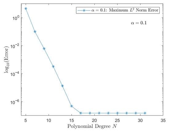
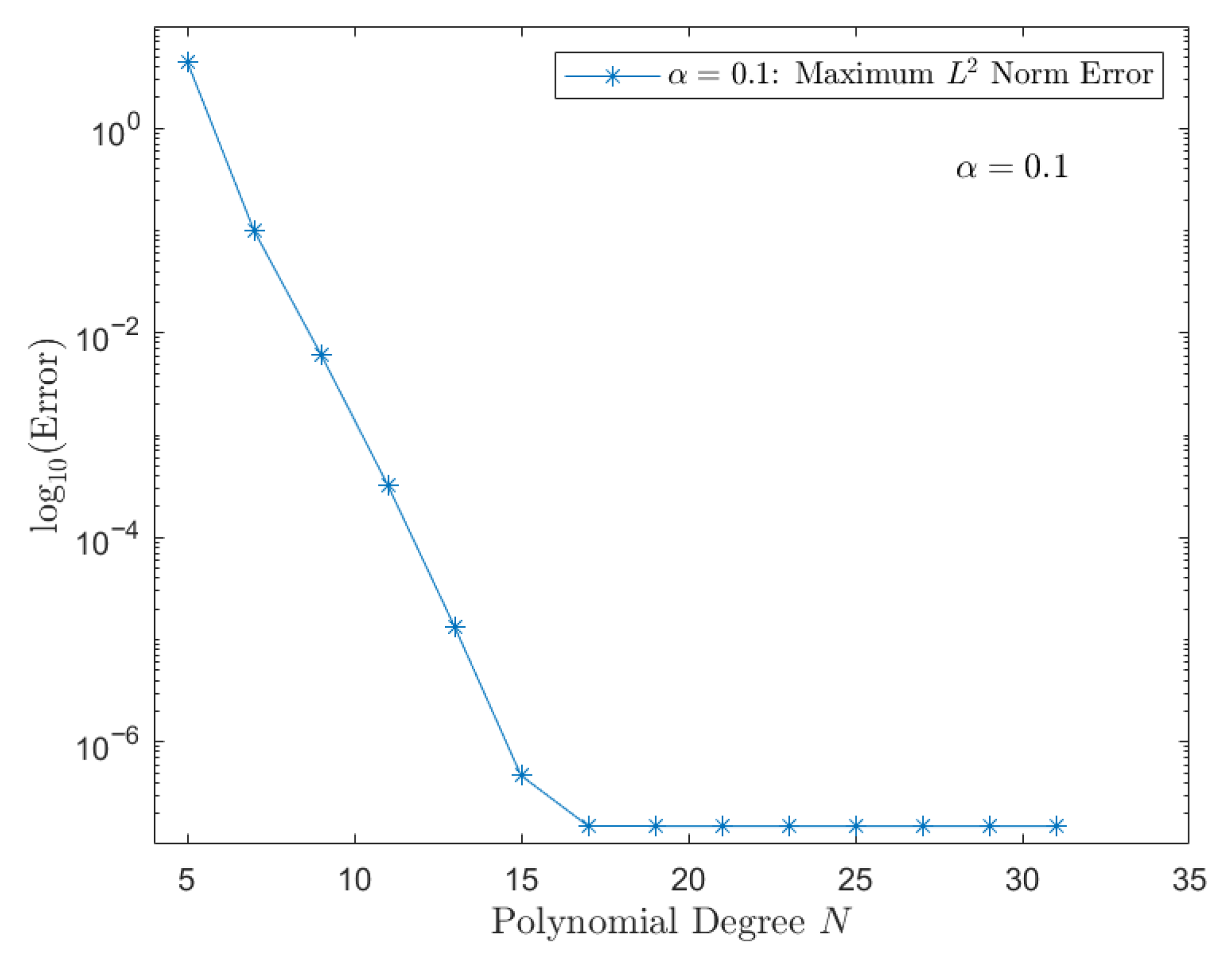
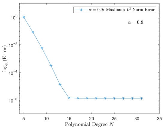
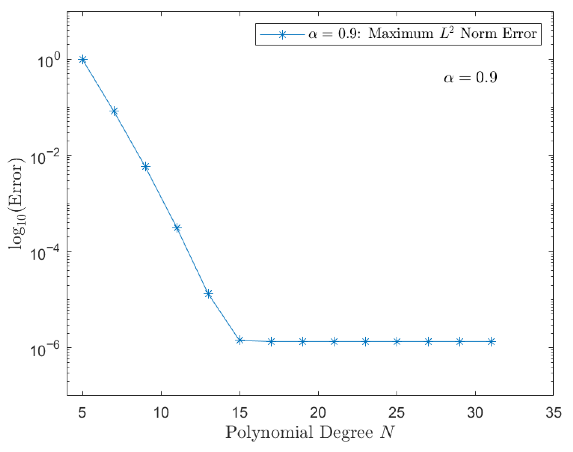
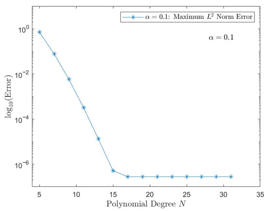
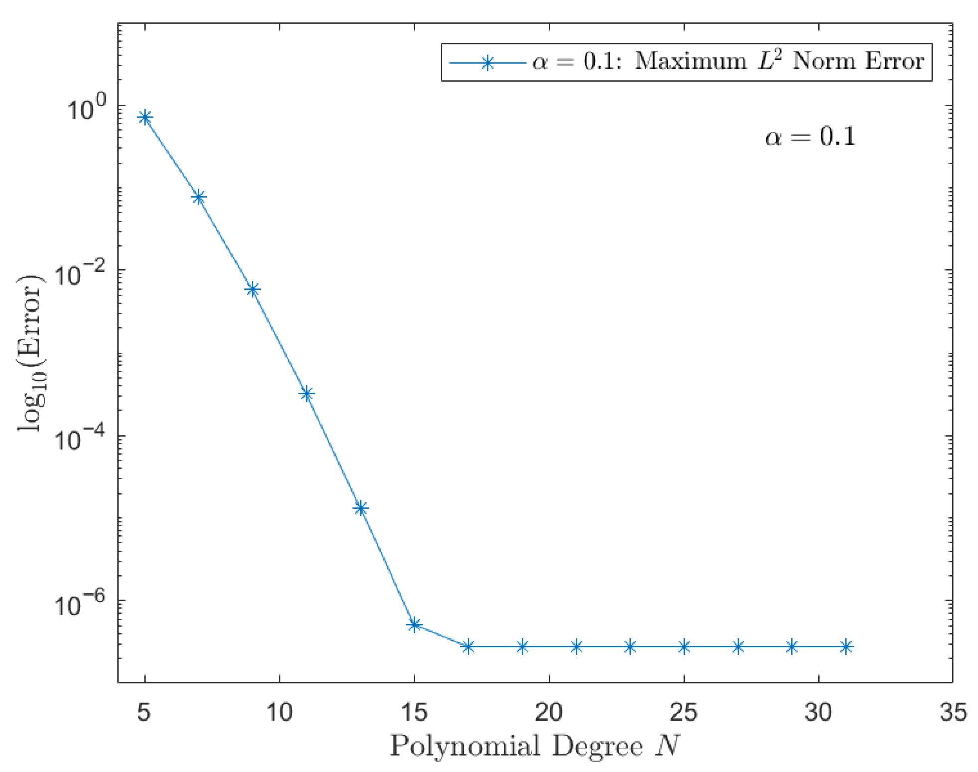
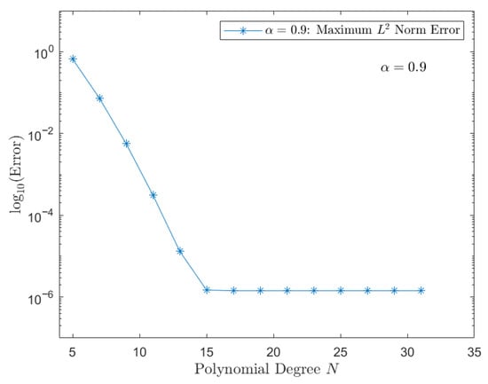
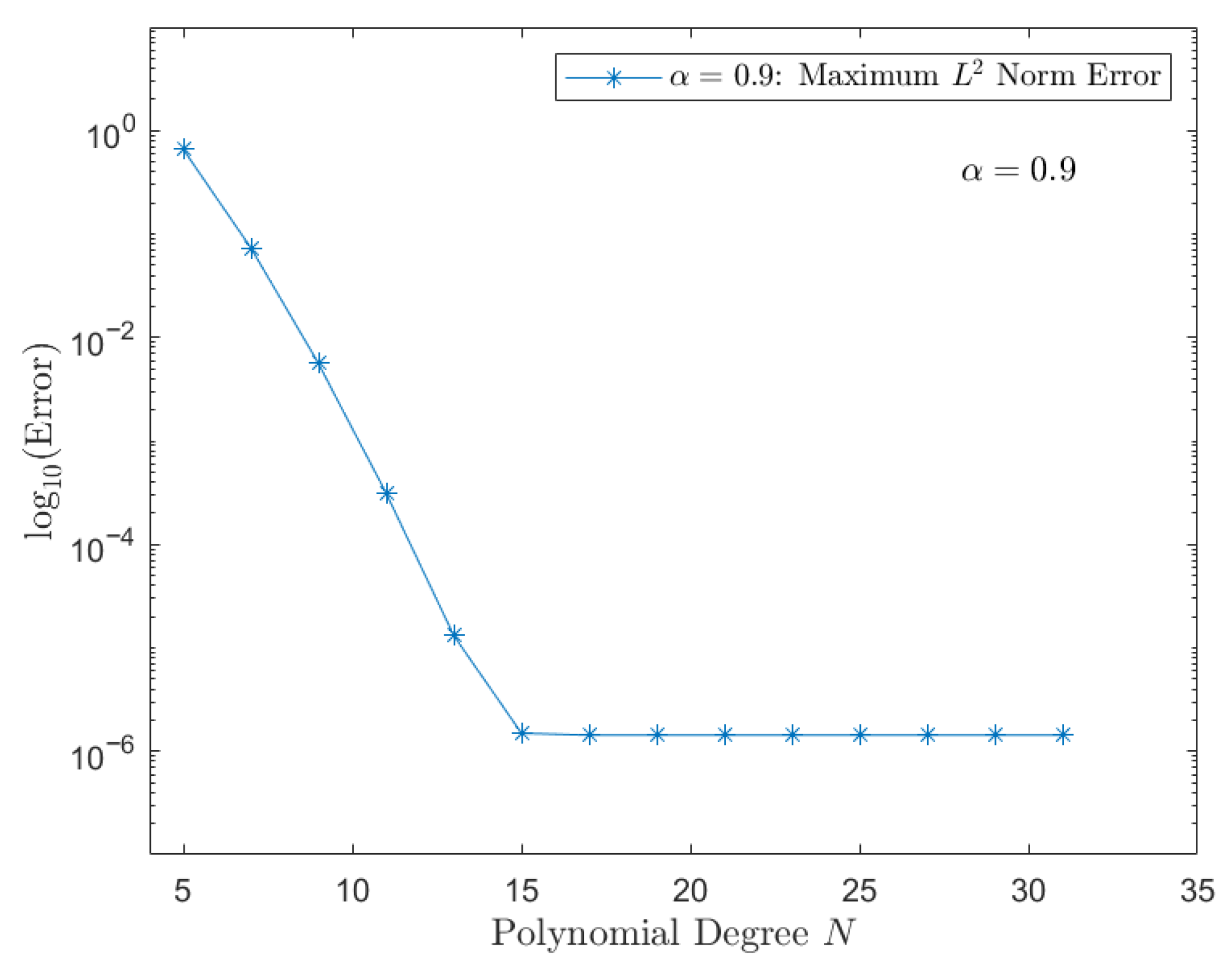
Next, we verify the spatial convergence rates by selecting $\tau$ small enough to avoid contamination of the temporal error. We take $\tau$ = 0.001. Figure 1 and Figure 2 describe the $L^2$ errors with respect to the polynomial degree N on a semi-log scale for different $\alpha$. The results demonstrate that the error decays exponentially, indicating that the method achieves spectral accuracy in space.

Figure 1. Errors versus the polynomial degree N for Example 1 ($\alpha =0.1$).

Figure 2. Errors versus the polynomial degree N for Example 1 ($\alpha =0.9$).

Example 2. 

Consider the following nonlinear time-fractional convection-diffusion equation:

$$\left\{\begin{array}{cc}{}_0{}^{C}D_t^{\alpha }u(x,t)-\mu {\mathsf{\partial }}_x^{2}u(x,t)+{\mathsf{\partial }}_{x}u(x,t)+u{(x,t)}^3=f(x,t),\hfill & (x,t)\in \Omega \times (0,T],\hfill \\ u(-1,t)=0,u(1,t)=0,\hfill & \\ u(x,0)=0,\hfill \end{array}\right.$$

where

$$f(x,t)={\displaystyle \frac{24t^{4-\alpha }}{\Gamma (5-\alpha )}}sin\left(2\pi x\right)+4\mu {\pi }^{2}sin\left(2\pi x\right)t^4+2\pi cos\left(2\pi x\right)t^4+{\left(t^{4}sin\left(2\pi x\right)\right)}^3.$$

The exact solution is $u(x,t)=t^{4}sin\left(2\pi x\right)$, $\mu =1$. To eliminate the influence of spatial errors, we choose a sufficiently large N and set $T=1$ and $N=64$. Table 2 displays the $L^2$ errors computed by the $L2$–$1_{\sigma }$ scheme for different values of $\alpha$. Evidently, the $L^2$ error achieves second-order temporal accuracy.

Table 2. Errors and temporal convergence rates for Example 2.

$\mathit{\tau }$	$\mathit{\alpha }=0.1$			$\mathit{\alpha }=0.5$			$\mathit{\alpha }=0.9$
	Error	Rate	CPU Time (s)	Error	Rate	CPU Time (s)	Error	Rate	CPU Time (s)
$1/8$	4.0319 × 10−3	–	0.0247	1.6317 × 10−2	–	0.0166	2.2200 × 10−2	–	0.0222
$1/16$	1.0467 × 10−3	1.9455	0.0366	4.1699 × 10−3	1.9683	0.0289	5.5845 × 10−3	1.9910	0.0258
$1/32$	2.6656 × 10−4	1.9733	0.0732	1.0530 × 10−3	1.9855	0.0526	1.3991 × 10−3	1.9970	0.0370
$1/64$	6.7255 × 10−5	1.9868	0.1377	2.6446 × 10−4	1.9934	0.0851	3.4995 × 10−4	1.9992	0.0619
$1/128$	1.6898 × 10−5	1.9928	0.2445	6.6250 × 10−5	1.9971	0.1560	8.7479 × 10−5	2.0001	0.1137
$1/256$	4.2487 × 10−6	1.9917	0.4745	1.6577 × 10−5	1.9988	0.2987	2.1862 × 10−5	2.0005	0.2660

We chose $\tau$ = 0.001. Figure 3 and Figure 4 describe the $L^2$ errors with respect to the polynomial degree N on a semi-log scale for different $\alpha$. The figures demonstrate that the errors decay exponentially; namely, we obtain spectral accuracy in space. All numerical results are consistent with our theoretical analysis.

Figure 3. Errors versus the polynomial degree N for Example 2 ($\alpha =0.1$).

Figure 4. Errors versus the polynomial degree N for Example 2 ($\alpha =0.9$).

7. Conclusions

We have constructed a spectral scheme for nonlinear time-fractional convection-diffusion equations. Theoretical analysis confirms that the scheme is unconditionally stable, meaning the numerical solution remains bounded for any spatial grid size N and temporal step $\tau$, which greatly enhances its practical applicability. The scheme also achieves a convergence rate of $O(N^{1-m}+{\tau }^2)$. The main contributions of this paper are: (i) the $L2$–$1_{\sigma }$ scheme, which significantly improves the temporal accuracy, and (ii) rigorous analysis of the existence and uniqueness of solutions to the fully discrete scheme. The methods we proposed can be applied to other equations as well as two-dimensional, three-dimensional, or even higher-dimensional equations. In future work, we aim to extend this framework to variable-order fractional derivative equations and coupled multi-physics systems, further broadening its scope of application.

References

- Sabatier, J.; Agrawal, O.P.; Machado, J.A.T. Advances in Fractional Calculus; Springer: Dordrecht, The Netherlands, 2007. [Google Scholar]
- Moaddy, K.; Momani, S.; Hashim, I. The non-standard finite difference scheme for linear fractional PDEs in fluid mechanics. Comput. Math. Appl. 2011, 61, 1209–1216. [Google Scholar] [CrossRef] [Scilit]
- Mainardi, F. Fractional Calculus: Some Basic Problems in Continuum and Statistical Mechanics. In Fractals and Fractional Calculus in Continuum Mechanics; Carpinteri, A., Mainardi, F., Eds.; Springer: Vienna, Austria, 1997; pp. 291–348. [Google Scholar]
- Grigorenko, I.; Grigorenko, E. Chaotic dynamics of the fractional Lorenz system. Phys. Rev. Lett. 2003, 91, 034101. [Google Scholar] [CrossRef] [Scilit] [PubMed]
- Rossikhin, Y.A.; Shitikova, M.V. Applications of fractional calculus to dynamic problems of linear and nonlinear hereditary mechanics of solids. Appl. Mech. Rev. 1997, 50, 15–64. [Google Scholar] [CrossRef] [Scilit]
- Metzler, R.; Klafter, J. The restaurant at the end of the random walk: Recent developments in the description of anomalous transport by fractional dynamics. J. Phys. A Math. Gen. 2004, 37, R161–R208. [Google Scholar] [CrossRef] [Scilit]
- Chen, C.; Jiang, Y.L. Lie group analysis and invariant solutions for nonlinear time-fractional diffusion-convection equations. Commun. Theor. Phys. 2017, 68, 295–300. [Google Scholar] [CrossRef] [Scilit]
- Li, C.; N’Gbo, N.G.; Su, F. Finite difference methods for nonlinear fractional differential equation with ψ-Caputo derivative. Phys. D Nonlinear Phenom. 2024, 460, 134103. [Google Scholar] [CrossRef] [Scilit]
- Abdulla, S.O.; Abdulazeez, S.T.; Modanli, M. Comparison of third-order fractional partial differential equation based on the fractional operators using the explicit finite difference method. Alex. Eng. J. 2023, 70, 37–44. [Google Scholar] [CrossRef] [Scilit]
- García, A.; Negreanu, M.; Ureña, F.; Vargas, A.M. On the numerical solution to space fractional differential equations using meshless finite differences. J. Comput. Appl. Math. 2025, 457, 116322. [Google Scholar] [CrossRef] [Scilit]
- Zhang, T.; Yin, Z.; Zhu, A. Block-Centered Finite-Difference Methods for Time-Fractional Fourth-Order Parabolic Equations. Fractal Fract. 2023, 7, 471. [Google Scholar] [CrossRef] [Scilit]
- Adel, E.; El-Kalla, I.L.; Elsaid, A.; Sameeh, M. An Adaptive Finite Element Scheme for Solving Space-time Riesz-Caputo Fractional Partial Differential Equations. Iran. J. Sci. 2025, 49, 1061–1073. [Google Scholar] [CrossRef] [Scilit]
- Qiu, W.; Fairweather, G.; Yang, X.; Zhang, H. ADI finite element Galerkin methods for two-dimensional tempered fractional integro-differential equations. Calcolo 2023, 60, 41. [Google Scholar] [CrossRef] [Scilit]
- Wang, Y.; Yin, B.; Liu, Y.; Li, H. Modified L1 Crank-Nicolson finite element methods with unconditional convergence for nonlinear time-fractional Schrödinger equations. Commun. Nonlinear Sci. Numer. Simul. 2025, 143, 108623. [Google Scholar] [CrossRef] [Scilit]
- Huang, C.; An, N.; Chen, H. Optimal pointwise-in-time error analysis of a mixed finite element method for a multi-term time-fractional fourth-order equation. Comput. Math. Appl. 2023, 135, 149–156. [Google Scholar] [CrossRef] [Scilit]
- Fouladi, S.; Mohammadi-Firouzjaei, H. Local discontinuous Galerkin method for the Riesz space distributed-order Sobolev equation. Eng. Anal. Bound. Elem. 2023, 155, 38–47. [Google Scholar] [CrossRef] [Scilit]
- Wang, J.; Yuan, S.; Liu, X. Finite Difference Scheme and Finite Volume Scheme for Fractional Laplacian Operator and Some Applications. Fractal Fract. 2023, 7, 868. [Google Scholar] [CrossRef] [Scilit]
- Yu, H.; Liu, F.; Li, M.; Anh, V.V. The non-uniform L1-type scheme coupling the finite volume method for the time–space fractional diffusion equation with variable coefficients. J. Comput. Appl. Math. 2023, 429, 115179. [Google Scholar] [CrossRef] [Scilit]
- Li, C.; Yuan, Y.; Yang, Q.; Sun, T. A Finite Volume Element Scheme Modified With Second-Order Upwind Fractional Step of Three-Dimensional Semiconductor Device Transient Behavior and Its Convergence Analysis. Numer. Methods Partial. Differ. Equ. 2025, 41, e23157. [Google Scholar] [CrossRef] [Scilit]
- Li, J.; Li, B.; Hu, Y. Solving a generalized fractional diffusion equation with variable fractional order and moving boundary by two numerical methods: FDM vs FVM. Phys. Scr. 2023, 98, 035204. [Google Scholar] [CrossRef] [Scilit]
- Wu, Z.; Zhang, X.; Wang, J.; Zeng, X. Applications of fractional differentiation matrices in solving Caputo fractional differential equations. Fractal Fract. 2023, 7, 374. [Google Scholar] [CrossRef] [Scilit]
- Adel, M.; Khader, K.; Algelany, S.; Aldwoah, K. An accurate approach to simulate the fractional delay differential equations. Fractal Fract. 2023, 7, 671. [Google Scholar] [CrossRef] [Scilit]
- Hu, H.; Cattani, P.; Mei, S. Hermite-Shannon-Cosine spectral method for fractional partial differential equations. Expert Syst. 2025, 42, e13370. [Google Scholar] [CrossRef] [Scilit]
- Abdelkawy, M.A.; Menaem, A.A.; Matoog, R.T.; Tedjani, A.H. Romanovski-Jacobi spectral collocation schemes for distributed order differential problems. Alex. Eng. J. 2024, 101, 98–107. [Google Scholar] [CrossRef] [Scilit]
- Behroozifar, M.; Sazmand, A. An approximate solution based on Jacobi polynomials for time-fractional convection-diffusion equation. Appl. Math. Comput. 2017, 296, 1–17. [Google Scholar] [CrossRef] [Scilit]
- Priyanka; Sahani, S.; Arora, S. An efficient fourth order Hermite spline collocation method for time fractional diffusion equation describing anomalous diffusion in two space variables. Comput. Appl. Math. 2024, 43, 193. [Google Scholar] [CrossRef] [Scilit]
- Mohammadi, S.; Ghasemi, M.; Fardi, M. A fast Fourier spectral exponential time-differencing method for solving the time-fractional mobile-immobile advection-dispersion equation. Comput. Appl. Math. 2022, 41, 264. [Google Scholar] [CrossRef] [Scilit]
- Londoño, M.A.; Giraldo, R.; Rodríguez-Cortés, F.J. An RBF-FD method for the time-fractional advection–dispersion equation with nonlinear source term. Eng. Anal. Bound. Elem. 2023, 151, 565–574. [Google Scholar] [CrossRef] [Scilit]
- Singh, A.; Kumar, S. Error analysis of a high-order fully discrete method for two-dimensional time-fractional convection-diffusion equations exhibiting weak initial singularity. Numer. Algorithms 2024, 99, 251–284. [Google Scholar] [CrossRef] [Scilit]
- Chawla, R.; Kumar, D.; Baleanu, D. Numerical investigation of two fractional operators for time fractional delay differential equation. J. Math. Chem. 2024, 62, 1912–1934. [Google Scholar] [CrossRef] [Scilit]
- Zeng, F.; Liu, F.; Li, C.; Burrage, K.; Turner, I.; Anh, V.V. A Crank-Nicolson ADI spectral method for a two-dimensional Riesz space fractional nonlinear reaction-diffusion equation. SIAM J. Numer. Anal. 2014, 52, 2599–2622. [Google Scholar] [CrossRef] [Scilit]
- Liu, H.; Lü, S. A high-order numerical scheme for solving nonlinear time fractional reaction-diffusion equations with initial singularity. Appl. Numer. Math. 2021, 169, 32–43. [Google Scholar] [CrossRef] [Scilit]
- Liu, H.; Lü, S. Numerical approximations for the nonlinear time fractional reaction-diffusion equation. Numer. Methods Partial. Differ. Equ. 2023, 39, 1355–1375. [Google Scholar] [CrossRef] [Scilit]
- Alikhanov, A.A. A new difference scheme for the time fractional diffusion equation. J. Comput. Phys. 2015, 280, 424–438. [Google Scholar] [CrossRef] [Scilit]
Disclaimer/Publisher’s Note: The statements, opinions and data contained in all publications are solely those of the individual author(s) and contributor(s) and not of MDPI and/or the editor(s). MDPI and/or the editor(s) disclaim responsibility for any injury to people or property resulting from any ideas, methods, instructions or products referred to in the content. |
© 2026 by the authors. Licensee MDPI, Basel, Switzerland. This article is an open access article distributed under the terms and conditions of the Creative Commons Attribution (CC BY) license.