


Abstract
Modern reliability experiments frequently face operational constraints that require balancing test duration, precision, and removal strategies, rendering classical censoring schemes inadequate for contemporary multidisciplinary applications. This study introduces a novel multi-progressive generalized Type-II censoring (MP-GC-T2) framework that unifies and extends existing progressive and generalized censoring structures through the integration of staged failure-proportion controls, dual temporal termination thresholds, and adaptive withdrawal of surviving units. The proposed mechanism provides enhanced flexibility in experiment design while retaining analytical tractability for statistical inference. Assuming Weibull lifetimes, we develop a complete inferential framework including maximum likelihood estimation, asymptotic interval construction, and Bayesian estimation via hybrid Metropolis–Hastings–Gibbs sampling with informative gamma priors, together with multiple interval estimation strategies for reliability characteristics. Extensive Monte Carlo investigations assess estimator bias, precision, coverage behaviour, and interval efficiency across diverse censoring configurations, demonstrating robustness and inferential gains relative to conventional schemes. Furthermore, optimal progressive-removal planning criteria are explored to guide practitioners in selecting censoring patterns that maximize inferential accuracy under practical constraints. The versatility and practical relevance of the MP-GC-T2 design are illustrated through applications to heterogeneous real datasets arising from clinical, chemical, geological, physical, and petroleum sciences, confirming its adaptability to distinct reliability structures and data-generation mechanisms. Collectively, the proposed methodology contributes a unified experimental and inferential platform that advances censoring design, reliability estimation, and cross-disciplinary statistical modelling.
Keywords:
multi-progressive generalized type-II; Weibull; progressive with failure proportion; optimum; reliability; failure rate; Bayesian; hybrid Markovian-based; optimization; multidisciplinary data analysis MSC:
62F10; 62F15; 62N01; 62N02; 62N05
1. Introduction
A generalized Type-II censoring (GC-T2), proposed recently by Long and Jiang [1], is a mixing of three independent traditional Type-II censoring (C-T2) designs that modifies the total number of observed failures to be adaptively adjusted according to the test duration and associated costs. Remember that the C-T2 test stops once a preassigned size of failures (say, m) has occurred out of a total of n tested units. Reliability examiners recognize that traditional C-T2 can lead to short test durations and reduced parameter estimation precision and data analysis accuracy due to early reaching the desired failures. Increasing the required number of failures can mitigate this issue, although it may increase the total duration of the experiment. Accordingly, in many actual life-testing scenarios, the proportions (for ) reflect low, medium, and high precision requirements for the acceptable and efficient inference, whereas (for ) represent lower and upper bounds on test duration that the experimenter can endure. Suppose that the experimenter first assigned the total value of n units, which are independent and identically distributed units.
The levels of time points and failure proportions must be specified in advance according to the experimenter’s expertise in such a way that and , where (for ) represent the length of failures recorded up to (for ). Let where denotes the biggest integer that is less than or equal to x.
Ultimately, by awaiting reaching the lifetime of the minimum size of failures from the total tested units n, the experimenter will collect one of the following ordered statistic patterns, namely:
- Set-1: when ;
- Set-2: when ;
- Set-3: when .
It is worth mentioning here that the GC-T2 can be used as a combined version of three classic C-T2 designs as follows:
- Data collection in Set-1 indicates that the test will stop at the highest failure size m when recording the lowest failure size k earlier, before the first threshold to reach the optimal number of failures m;
- Data collection in Set-2 indicates that the test will stop at the moderate failure size r when recording the lowest failure size k within the smaller and larger test time limits to balance costs and time expenditure;
- Data collection in Set-3 indicates that the test will stop at the lowest failure size k when recording the lowest failure size k later than the largest time period to complete the test to preserve the overall cost allocated to the test, particularly when there is one or more units under test with extreme ages.
Progressive Type-II censoring (PC-T2) has become an essential tool in modern lifetime and reliability analysis, offering a flexible experimental structure that overcomes many limitations of conventional censoring designs. Unlike classical censoring designs, and following the philosophy of progressive removal theory, in which, after a specified number of failures, the experiment is ended, progressive plans allow the experimenter to strategically withdraw surviving units at predetermined failure times. Several versions of such schemes have been suggested; see, for example, Balakrishnan and Cramer [2]. Accordingly, PC-T2 provides richer inferential information than conventional C-T2 by preserving both the ordering and timing of failures while maintaining control over the removal of surviving units. These characteristics make it particularly valuable in engineering reliability assessment, accelerated life testing, biomedical studies, and industrial quality control, where experimental precision must be balanced against operational cost.
Over the past two decades, PC-T2 schemes have undergone several refinements aimed at improving experimental efficiency, regulating test duration, and enhancing statistical precision. Notably, the hybrid PC-T2 (H-PC-T2) introduced by Kundu and Joarder [3], the adaptive PC-T2 (A-PC-T2) proposed by Ng et al. [4], and the improved A-PC-T2 (IA-PC-T2) developed by Yan et al. The work in [5] represents three major advancements in this direction. Each of these censoring mechanisms was designed to address specific limitations related to time constraints, removal strategies, and estimation accuracy, thereby broadening the practical applicability of progressive censoring in reliability and lifetime studies, specifically:
- An H-PC-T2 imposes a strict upper limit on the test duration by terminating the experiment at the time or when is reached, whichever occurs first. This design guarantees time control but often results in observing fewer failures than desired.
- An A-PC-T2 allows the test to proceed beyond the fixed inspection time , ensuring that all pre-specified failures m are eventually observed. Although this flexibility increases the amount of available failure information, it may also cause the test to extend for an excessively long duration when the items under study are highly reliable.
- An IA-PC-T2 introduces two finite time thresholds, and , creating a controlled adaptive window for test continuation. This design generalizes both H-PC-T2 and A-PC-T2, providing better control over test duration and efficiency.
Although the IA-PC-T2 design offers substantial flexibility, it often yields a relatively small observed sample size (say, m) when the maximum experimental duration (say, ) is constrained by practical or economic considerations. This reduction in observed failures may lead to less efficient statistical inference. Motivated by these considerations, we extend the GC-T2 (by Long and Jiang [1]) to allow the experimenter to withdraw one or more surviving units during testing. This added allowance enhances the flexibility of IA-PC-T2 by enabling it to accommodate three levels of observed failure sizes, k, r, and m, determined by their respective proportions . The proposed modification of the GC-T2 mechanism offers several benefits, including reduced testing time, suitability for high-cost or destructive experiments, and efficient use of limited testing resources. A notable advantage is that the new censoring plan can be viewed as a general plan of C-T2, GC-T2, and PC-T2, among other related schemes. Henceforth, we refer to this censoring plan as a multi-progressive GC-T2 (MP-GC-T2) scheme, which will be detailed in the next section.
In contemporary lifetime and reliability testing, researchers face increasing pressure to balance statistical accuracy with practical constraints, such as limited test duration, high experimental costs, and the need to control the number of observed failures. Classical C-T2 and PC-T2 designs, while foundational, often prove inadequate in modern engineering and biomedical contexts where early failures occur unpredictably, or test units are expensive and destructively tested. Although recent advancements, such as H-PC-T2, A-PC-T2, and IA-PC-T2 plans, provide partial time control and enhanced flexibility, they still suffer from limitations such as small effective sample sizes, restricted removal strategies, and insufficient adaptability to multiple precision levels. At the same time, GC-T2 introduces multiple failure-proportion stages but lacks the ability to remove surviving units progressively. Motivated by the need for a unifying censoring structure that flexibly regulates time, adapts failure proportions, and permits progressive withdrawals, this study develops a new MP-GC-T2 strategy. This system enables transitions among three effective sampling sizes and two temporal thresholds, contingent upon the experimenter’s available funding and the maximum duration they are able to tolerate. It also integrates the strengths of GC-T2 and PC-T2 families, offering an experimentally practical and statistically efficient design that enhances data richness while maintaining strict control over duration, cost, and precision level. However, the main contributions can be summarized sevenfold, as follows:
- Proposes a novel MP-GC-T2 censoring scheme that integrates multi-stage failure proportions, progressive removals, and dual test-time thresholds. The proposed design unifies and generalizes several well-known censoring plans, including C-T2, GC-T2, PC-T2, H-PC-T2, A-PC-T2, and IA-PC-T2, as special cases.
- Derives the maximum likelihood estimator (MLE) of (for fixed ) and the profile likelihood estimator of , together with two types of asymptotic confidence intervals (ACIs) based on the normal approximation and its log-transformed version for both model parameters and reliability measures.
- Develops a Metropolis–Hastings-within-Gibbs sampling algorithm to implement Bayesian inference under independent gamma priors.
- Constructs two asymptotic confidence intervals (normal and log-transformed) as well as two Bayesian credible intervals, namely the equal-tailed Bayesian credible interval (BCI) and the highest posterior density (HPD) interval.
- Conducts extensive Monte Carlo simulations to evaluate bias, mean squared error, average interval length, and coverage probability of the proposed methods under various censoring schemes and design configurations.
- Develops a comprehensive optimum-plan framework that determines progressive removal patterns and failure-proportion settings that minimize estimator variability and improve interval performance, thereby facilitating the selection of an efficient censoring configuration under practical time and cost constraints.
- Analyzes five real datasets arising from clinical, chemical, geological, physical, and petroleum applications to demonstrate the flexibility of the proposed method across diverse hazard structures, censoring levels, and experimental conditions. These applications illustrate that the MP-GC-T2 plan is broadly applicable and not confined to a specific scientific domain.
The remaining sections of the paper are organized as follows. Section 2 presents the MP-GC-T2 model together with its likelihood formulation. Section 3 and Section 4 develop the classical and Bayesian estimation frameworks, respectively. Numerical comparisons are provided in Section 5. Section 6 discusses two physically relevant applications. Optimal assessments and associated criteria are examined in Section 7. Finally, Section 8 offers concluding remarks, potential research, and recommendations.
2. The MP-GC-T2 Scheme
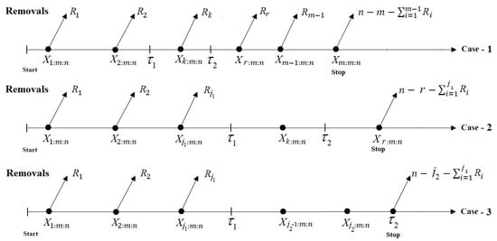
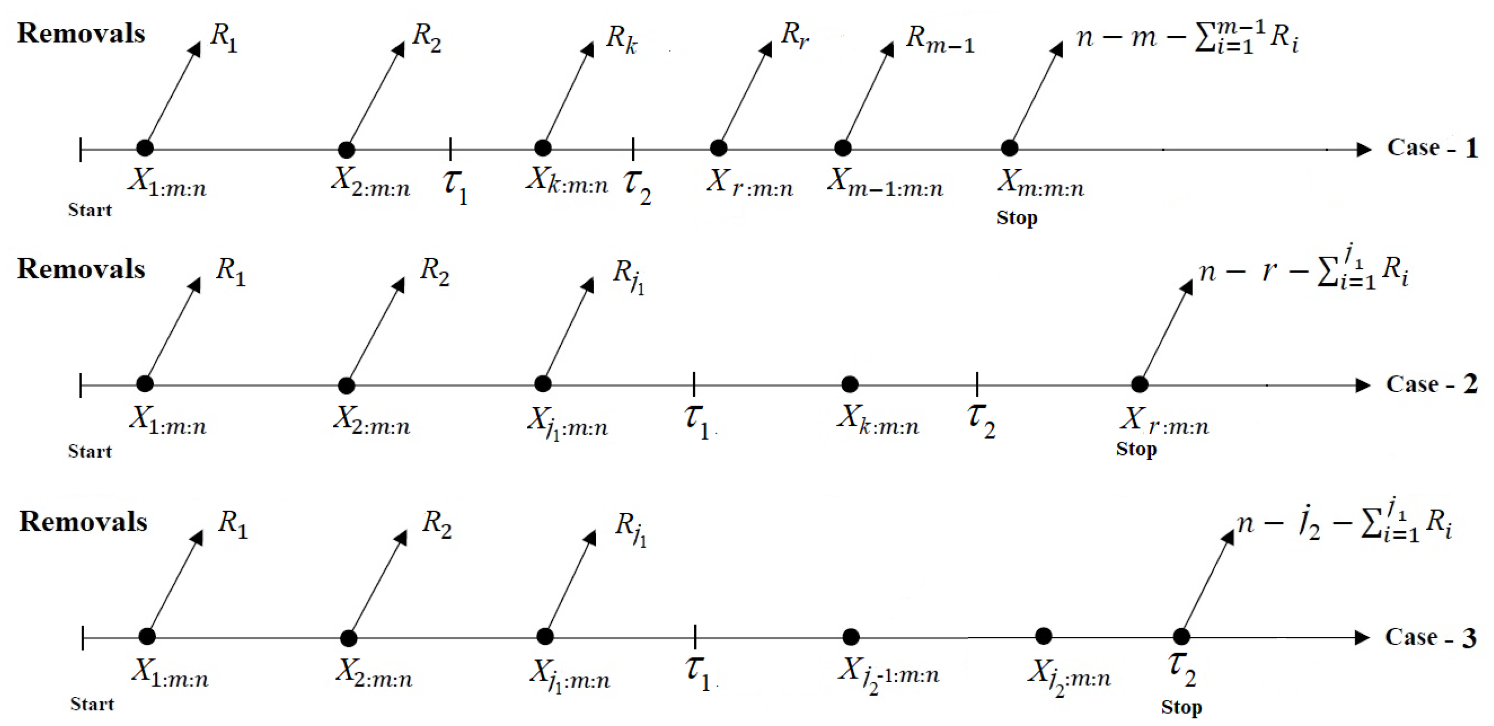
Let denote the number of observed failures, and let represent a preassigned progressive pattern satisfying . The number of units withdrawn at each stage, , is fixed in advance, whereas the specific units removed are chosen uniformly at random from the surviving units still under observation. Given the observed failure history up to that point, the withdrawal mechanism is assumed to be independent of the remaining lifetimes. This plan depends on three failure proportions changed according to two finite time thresholds where , to provide better control over the overall test duration. At , the experimenter randomly removes units from the remaining surviving units. Following the second failure, , units are randomly withdrawn from the remaining units, and this procedure continues for all planned removals. At three different stopping conditions (say, ), all remaining units (say, ) and associated data collections (say, ) are removed (see Table 1). In this table and elsewhere, we shall use instead of for simplicity. For further clarification, the procedures for MP-GC-T2 cases are shown in Figure 1.
Table 1.
Stopping points and data collections of MP-GC-T2 plan.
Figure 1.
Schematic diagram of the MP-GC-T2 scheme.
The joint likelihood function (LF), , of a sample of size , denoted by , obtained by MP-GC-T2 from a population characterized by PDF and CDF can be formulated as follows:
where
It is important to emphasize that the MP-GC-T2 scheme produces three possible censoring scenarios, corresponding to early, intermediate, and late realizations of the minimum required failure size of k. The observed data consist of the failure times together with associated removals, symbolized by where , depending on the realized value of relative to . The proposed test operates by controlling the time of the observed minimum number of failures. If the maximum threshold is reached before at least k failures occur, the experiment is terminated immediately. Otherwise, depending on , an adaptation stage is triggered to collect additional failure information by extending the observation period to obtain a moderate-sized failure r or a larger-sized failure m. It should be noted here that, to ensure the ideal test time , which represents the longest test time that can be tolerated to continue, beside multiple choices for the number of failures, each ensuring that the inference remains valid and accurate, we stopped the experiment when the test time exceeded up to without reaching the minimum failure time . This censoring plan balances the trade-off between inferential accuracy and testing duration to improve estimation precision while controlling overall experimental time and cost. This formulation also unifies staged failure-proportion control, dual time constraints, and progressive withdrawals within a single stopping-time–based censoring framework. Recall that the MP-GC-T2 design can be regarded as a generalization of several well-known censoring mechanisms. Specifically, from (1), it can be seen that the proposed design encompasses, as special cases, a number of existing censoring strategies; see Table 2.
Table 2.
Special censoring schemes from the MP-GC-T2 plan.
Corollary 1.
The likelihood function of the MP-GC-T2 plan expressed in Equation (1) is obtained by conditioning on the realized terminal failure size A and the predetermined progressive removal scheme , where the removal horizon B depends on the realized censoring case. Under this conditioning, the likelihood admits a factorization into three components:
- (i)
- The joint density of the observed failure times,
- (ii)
- The survival contributions corresponding to progressive removals up to stage B, and
- (iii)
- The final right-censoring term evaluated at the termination time .
The combinatorial factor arising from the risk set sizes depends only on and is free of the model parameter vector θ; hence, it can be absorbed into a normalizing constant. Consequently, the resulting likelihood kernel provides a unified analytical representation for all three censoring cases of the MP-GC-T2 scheme; see Appendix A for details.
3. Likelihood Estimation
The Weibull distribution stands out as a versatile and powerful tool in reliability analysis, survival studies, and engineering, offering unprecedented flexibility through its shape parameter and scale parameter . By tuning , the distribution can seamlessly capture increasing, decreasing, or constant hazard behaviors, while governs the characteristic life, allowing precise modeling of systems with widely varying lifetimes. Its elegant mathematical structure enables efficient estimation, inference, and predictive analytics, making it an indispensable tool for both theoretical development and practical applications. As such, the Weibull distribution continues to drive innovation in reliability modeling, offering a rigorous yet flexible framework for understanding and predicting lifetime behaviors of diverse systems.
A lifespan random variable X is assumed to have a Weibull, where , if its respective probability density function (PDF), , cumulative distribution function (CDF), , and hazard rate function (HRF), , are:
and
where the corresponding reliability function (RF), , and hazard rate function (HRF), , of X at a mission time t are given, respectively, by:
When a dataset is collected upon the MP-GC-T2 plan, this section focuses on deriving the ML estimation and corresponding two types of asymptotic interval bounds of the Weibull parameters and , and associated reliability time functions and .
3.1. The ML Estimators
This part is devoted to the analytical derivations for the MLEs of and , denoted by and , respectively. From (2) and (3), the LF (1) and log-LF can be written as:
and
respectively, where .
Using (6), beyond equating the first derivative result of to zero, the MLE can be expressed (for fixed ) as follows:
To derive the MLE , by substituting (7) into (6), the profile log-LF (say, ) of can be easily derived as follows:
Accordingly, by maximizing (8) with respect to , the MLE can be developed as a function of as follows:
where .
After solving (9) for using any numerical optimization routine, the corresponding MLE of can be computed immediately by substituting into the expression given in (8).
Corollary 2.
The MLE of λ can be obtained in closed form once the MLE of β is available. Therefore, the existence and uniqueness of are guaranteed if and only if exists and is unique.
Proof.
Differentiate (8) with respect to , get the likelihood equation , as
It is clear that is strictly decreasing in . For , the Cauchy–Schwarz inequality shows that
which implies that is strictly increasing in , where
Moreover, possesses a finite upper bound; specifically, by taking , we get
Ultimately, combining the fact that possesses a finite upper limit with the fact that decreases monotonically to zero whereas increases monotonically, we conclude that the likelihood Equation (8) has a unique solution. Hence, the MLE of exists and is unique, and so is the corresponding estimator . □
Corollary 3.
The MLEs and of two reliability metrics of life, and , respectively, for are obtained directly from the invariance property by replacing β and λ with their estimates and , respectively.
3.2. The ACI Estimators
This subsection focuses on introducing two kinds of ACIs of , , , and ; the first using the normality approximation of MLE (referred to as NA-ACI) and the other based on the normality approximation for the logarithm of MLE (referred to as NL-ACI). First, to derive the NA-ACI of , , , or , the asymptotic variance–covariance matrix (VCM), which is computed as the inverse of the Fisher information matrix (FIM), should be derived first. Accordingly, from (6), we begin by evaluating the second-order partial derivatives of the log-LF (say, for ) with respect to and as follows: , , and Subsequently, from for , the VCM (say, ) of and becomes
We require estimates of the variances of and (denoted by and , respectively) in turn to find their NA-ACI estimates. These variances are approximated using the delta method, which provides large-sample variance estimates for nonlinear functions of parameter estimators by employing a first-order Taylor series expansion. This approach yields tractable approximations for standard errors of complex reliability measures; see Greene [7] and Oehlert [8].
We first obtain the gradient terms of and from and , namely:
and
Hence, the quantities and are given directly by
respectively. Accordingly, using the normal approximation of the MLEs for , the two–sided NA-ACI estimators of are given by
where and denotes the upper -quantile of the standard normal distribution.
Meeker and Escobar [9] introduced an alternative procedure for constructing ACI in which the MLE is first transformed using its natural logarithm before constructing the associated interval estimate. This approach, known as the NL-ACI, ensures that all resulting bounds are strictly positive for parameter(s) that have values in the positive domain. They also stated that this method provides more stable and practically interpretable intervals, especially in moderate and small samples. The improvement stems from the log transformation’s ability to mitigate the skewness often observed in the sampling distribution of the MLEs. Hence, the two-sided NL-ACI estimators of (for ) are given by
or equivalent,
Corollary 4.
Recall that the lifetimes observed under the proposed MP-GC-T2 plan are assumed to follow a Weibull lifespan model. Accordingly, statistical inference is performed conditionally on the realized terminal failure size A and the progressive removal configuration . To clarify the behavior of the likelihood function and its derivatives under this complex censoring structure, we summarize below several analytical considerations:
- (i)
- Identifiability: For the Weibull parameter vector , identifiability requires that the score equations admit a unique solution. This condition is satisfied whenever at least two distinct failure times are observed, that is, and for some . However, as A decreases, the likelihood surface becomes increasingly flat in the β-direction, leading to a loss of practical identifiability in finite samples, despite theoretical identifiability.
- (ii)
- Information loss under heavy censoring: The conditional Fisher information element associated with the shape parameter β decreases as the number of observed failures A decreases and as the censoring weight concentrates at the terminal failure time . In the extreme case and , indicating that the shape parameter becomes weakly identifiable and numerically unstable.
- (iii)
- Implications for inference: These analytical observations explain the increased estimator variability and occasional instability observed in the simulation study under high censoring levels. They further justify the use of Bayesian regularization and prior information to stabilize inference in heavily censored regimes.
4. Bayesian Estimation
This section derives the Bayesian point and Bayesian credible intervals (BCIs) and greatest posterior density (HPD) intervals for , , , and . The derivations are based on the assumption that the Weibull() parameters are stochastically independent and include previous information via the associated prior models. Among several prior options, the gamma conjugation prior is extensively used due to its flexibility (see Kundu [10]). Owing to its mathematical convenience and its ability to reflect diverse prior beliefs for positive parameters, the gamma density works as an superior priori law. Suppose and are assumed a priori independent and distributed with and , respectively.
Consequently, the prior PDF of , denoted by , is given by
In Bayes’ theorem, the joint posterior PDF of (say, ) is given by
where From (6) and (11), the posterior PDF (12) of becomes
The squared-error loss (SEL) function is one of the most widely used symmetric losses. According to it, the Bayes estimator of , , , or , say for instance, denoted by , is defined as the posterior expectation of as follows:
However, due to the nonlinear and complex structure of the posterior distribution in (14), closed-form Bayes estimators for or corresponding BCI/HPD estimators cannot be derived. Accordingly, the MCMC sampling scheme is adopted to obtain the Bayes estimator and the associated credible intervals for each unknown subject. Implementing this procedure requires the derivation of their conditional posteriors as follows:
and
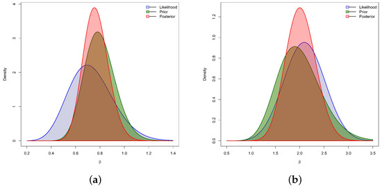
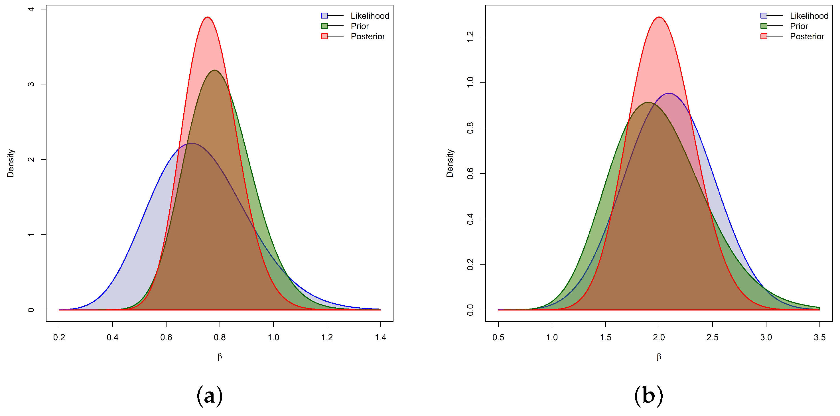
respectively. It is evident, from (16), that the samples of gathered from the posterior PDF are feasible and can be gathered directly from the gamma iterative sampler. In contrast, the posterior PDF (15) of does not correspond to any standard statistical model. To illustrate this, a single MP-GC-T2 dataset is generated from Weibull (with and ) and Weibull (with and ) under , , , and . Figure 2 reveals that the fitted PDF for and —considering likelihood (gray), prior (green), and posterior (red)—approximately follows a normal distribution.
Figure 2.
The likelihood, prior, and posterior density shapes of . (a) Weibull . (b) Weibull.
The posterior distribution (15) is considerably more concentrated than the corresponding informative gamma prior and closely tracks the likelihood functions, indicating that the observed data provide substantial information to update prior beliefs for across different configurations provided. Consequently, we use the Metropolis–Hastings (MH) algorithm (to update the shape parameter ) along with Gibbs sampling (to update the scale parameter ) as a procedure listed in Algorithm 1.
| Algorithm 1 The MH-Gibbs Sampling |
|
5. Monte Carlo Simulations
This part evaluates the effects of the previously obtained theoretical conclusions, including both the classical and Bayesian methods of estimation, as well as their related asymptotic and credible intervals, using comprehensive Monte Carlo computer simulation investigations.
5.1. Simulation Designs
We replicate the MP–GC–T2 scheme 1000 times by the generating steps depicted in Algorithm 2 from the and models under multiple configurations of the failure ratios , thresholds , total sample sizes n, and objective failure sizes . To assess the sensitivity of inference to the failure-proportion controls embedded in the MP-GC-T2 scheme, we consider multiple combinations of satisfying . Varying these thresholds systematically alters the probability of early, intermediate, and late termination, thereby impacting the effective number of observed failures. Specifically, we consider:
| Algorithm 2 The MP–GC–T2 Sampling |
|
For each value of n, the failure sizes and PC-T2 are determined based on the specified failure ratios, as summarized in Table 3. The censoring configurations (listed in Table 3) are designed to represent distinct censoring regimes rather than arbitrary settings. Specifically, the selected configurations correspond to low, moderate, and heavy censoring levels, as quantified by the realized terminal failure size A relative to the full sample size n. This stratification ensures that estimator performance is evaluated across a broad spectrum of practical testing scenarios. To further illustrate estimator performance, we evaluate the RF and HRF at . The true values of at are for the model and for the model, respectively. To investigate the impact of gamma prior specifications on Bayesian inference for the Weibull parameters , , , and , we consider two distinct informative sets of hyperparameters, for , for each given Weibull model. Notably, the proposed priors 1 and 2 for or follow the approach of prior mean and prior variance described by Kundu [10]. This methodology allows the selection of prior parameters such that the prior expectation of each informative set coincides with the corresponding predetermined true value of the parameter. The considered sets of hyperparameters , namely:
Table 3.
Censoring designs in numerical comparisons.
- : Prior-1: ; Prior-2: ;
- : Prior-1: ; Prior-2: .
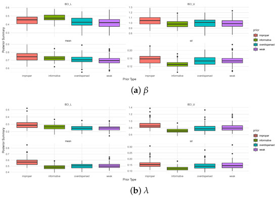
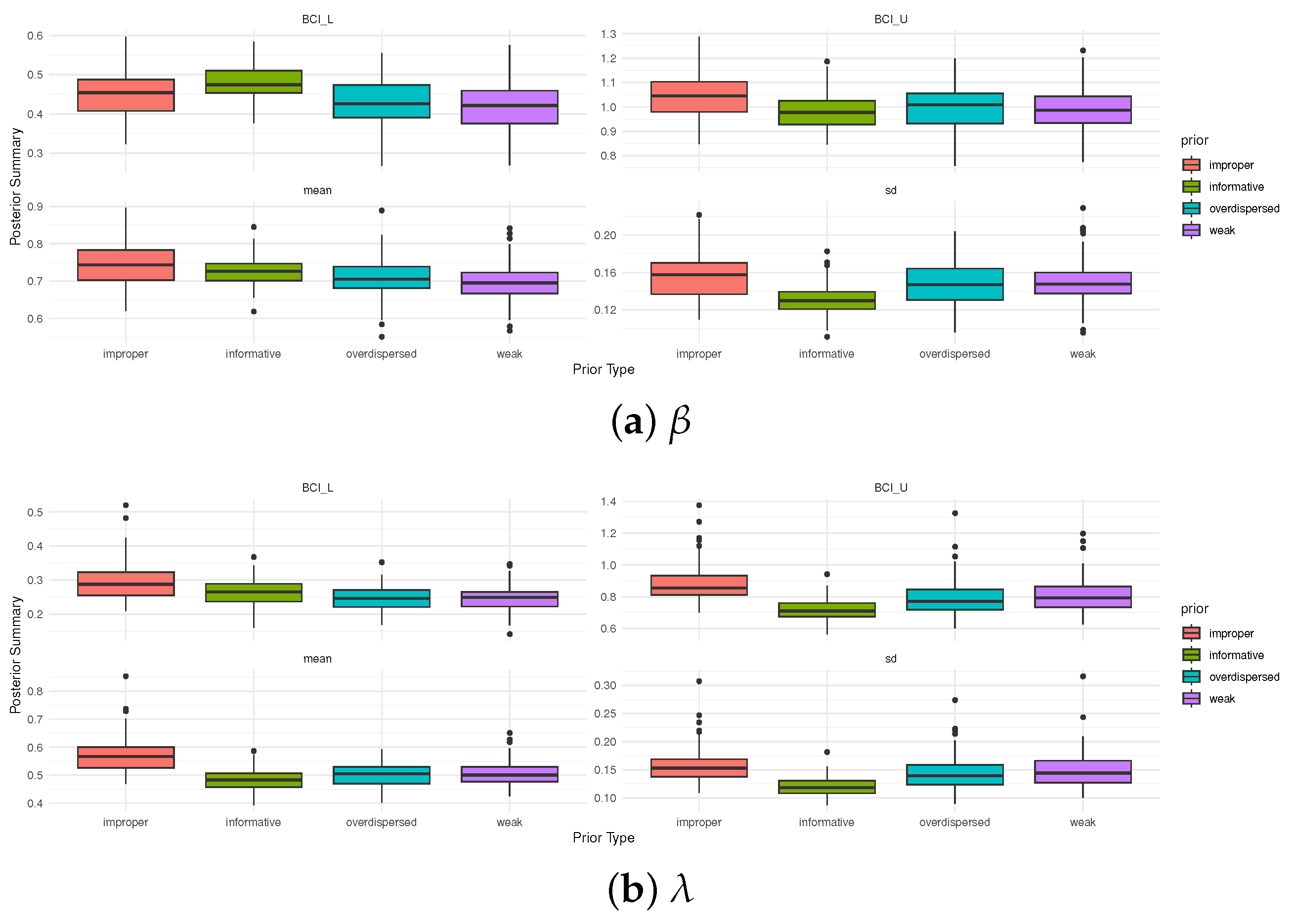
A sensitivity analysis of the posterior distributions is performed to assess the robustness of the Bayesian results, namely the posterior means, standard deviations, and credible intervals, under alternative prior choices. Such an investigation is particularly relevant in the presence of censoring and model complexity, where prior assumptions may exert a non-negligible influence on inference. To this end, 1000 T2-GPHC-BRR samples are simulated from a distribution with and the T1[R1] scheme, and posterior behavior is examined under four prior formulations: an informative prior (Prior-1), an improper prior (e.g., for both and ), an overdispersed prior (e.g., and for and , respectively), and a weakly informative prior (e.g., for both parameters). The results displayed in Figure 3 suggest that the posterior summaries demonstrate only moderate sensitivity to the choice of prior. The informative prior produces the shortest BCIs and the smallest posterior dispersion, indicating improved estimation accuracy. By comparison, the improper and weakly informative priors yield slightly broader intervals and larger posterior variability, whereas the overdispersed prior generates the most diffuse posterior distributions. Overall, these findings indicate that the proposed informative prior provides an effective compromise between robustness and efficiency within the considered censoring framework.
Figure 3.
Sensitivity analysis for the simulated posterior estimates of and from .
All numerical analyses were carried out in R (version 4.2.2) using two dedicated packages. The MLEs and their 95% ACIs, obtained under both NA and NL transformations, were computed with the maxLik package (Henningsen and Toomet [11]). Taking and , the Bayesian point estimates, together with BCI/HPD, were produced using the coda package (Plummer et al. [12]). Computational efficiency is assessed by recording the average runtime per simulation replication for each censoring configuration. Mostly, the average runtime ranged within 30 and 60 s per replication, reflecting the larger effective sample size and increased numerical optimization cost.
To assess the estimators of , , , and (say, ), we consider the following measures:
- Root Mean Squared Error
- Average Relative Absolute Bias
- Average Interval Length
- Coverage Probability:where is an indicator.
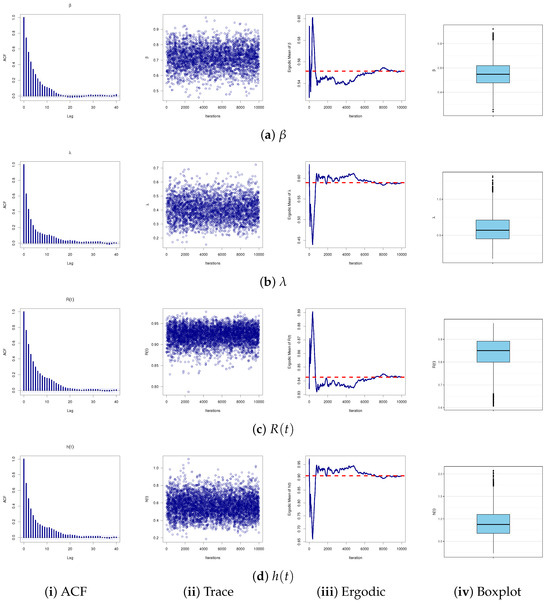
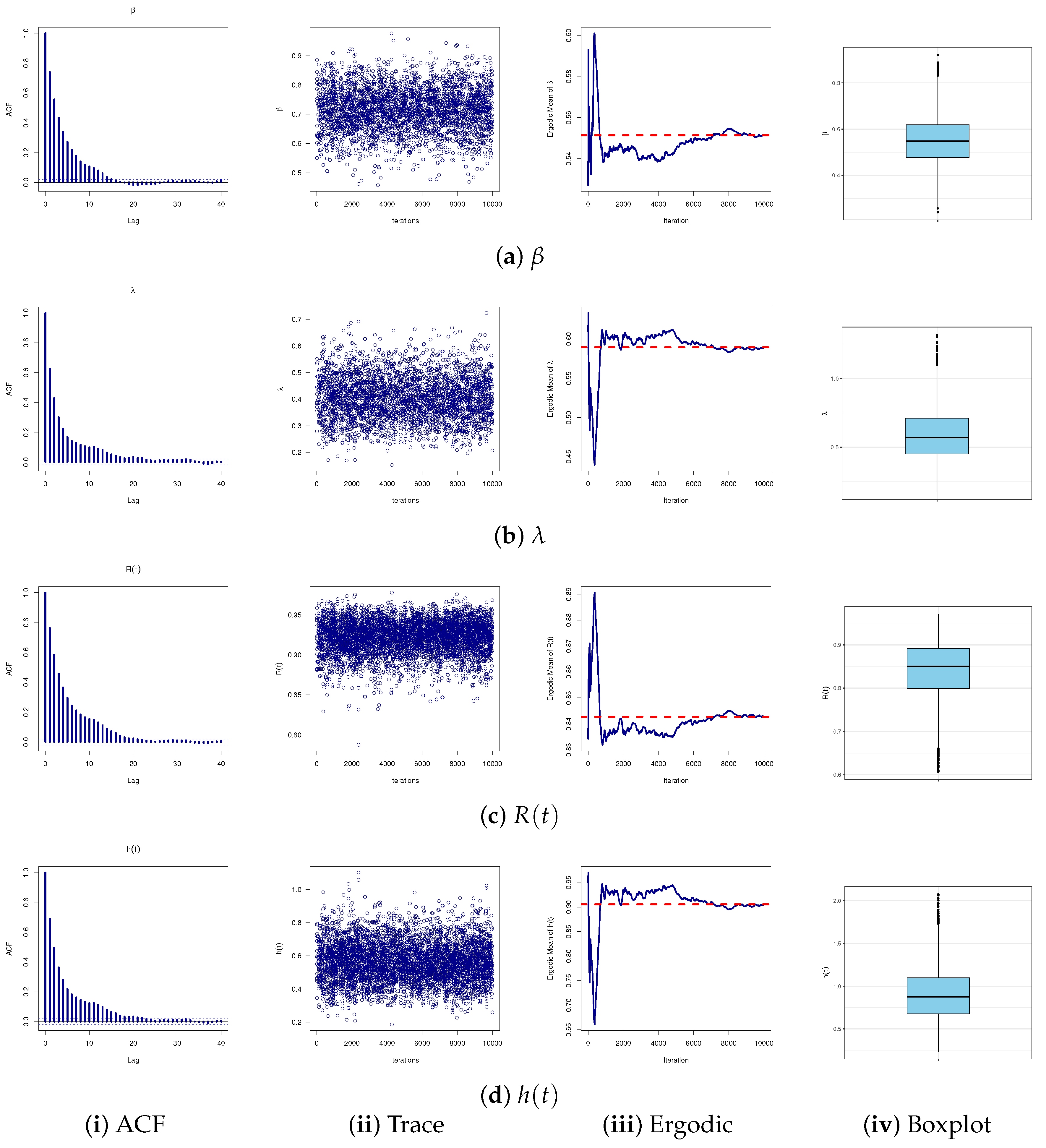
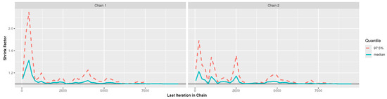
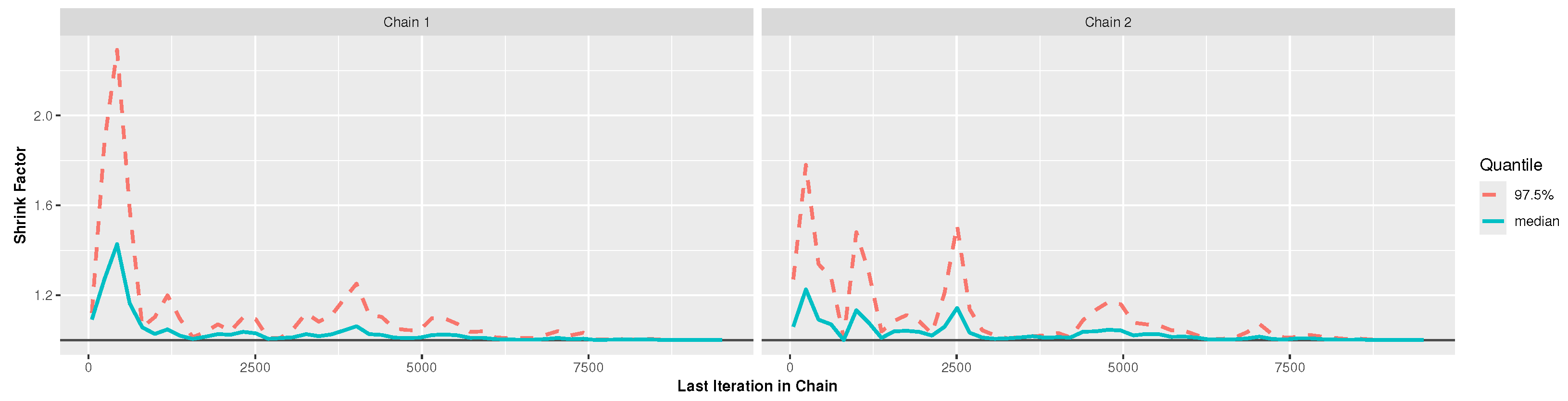
To assess the performance and convergence behavior of the MH–Gibbs algorithm used to estimate the parameters , , , and of the Weibull model, a comprehensive set of MCMC diagnostics is produced. For each parameter, four complementary diagnostics are examined (see Figure 4), namely: (i) autocorrelation function (ACF), (ii) trace, (iii) ergodic (cumulative mean), and (iv) boxplot of the post–burn-in samples. Together, these diagnostics allow for a rigorous evaluation of chain stability, mixing efficiency, and convergence to the stationary posterior distribution. The ACF plot highlights the dependence structure within the chain; the trace plot illustrates mixing and potential drift; the ergodic mean plot demonstrates asymptotic stabilization toward the posterior expectation; and the boxplot summarizes the empirical posterior distribution. A consistent pattern of rapid autocorrelation decay, stable traces, and quickly flattening ergodic averages across all parameters indicates satisfactory convergence of the MCMC sampler. All subplots in Figure 4 indicate that the MCMC diagnostics for , , , and provide robust convergence, with the ACF showing rapid decay, the trace plot exhibiting stable stationarity, and the ergodic mean stabilizing early, all reflecting efficient mixing. Additionally, the compact posterior in the boxplot confirms the strong, stable, and accuracy of the MCMC estimates for each unknown quantity. In contrast, the Brooks–Gelman–Rubin (BGR) diagnostic (shown in Figure 5) reveals that there is no statistically significant difference in the variances within and between the generated Markov chains.
Figure 4.
Four MCMC diagnostics of , , , and a simulated MP–GC–T2 dataset from .
Figure 5.
The BGR diagnostic using a simulated MP–GC–T2 dataset from .
5.2. Simulation Results
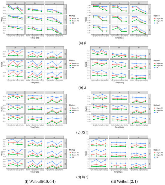
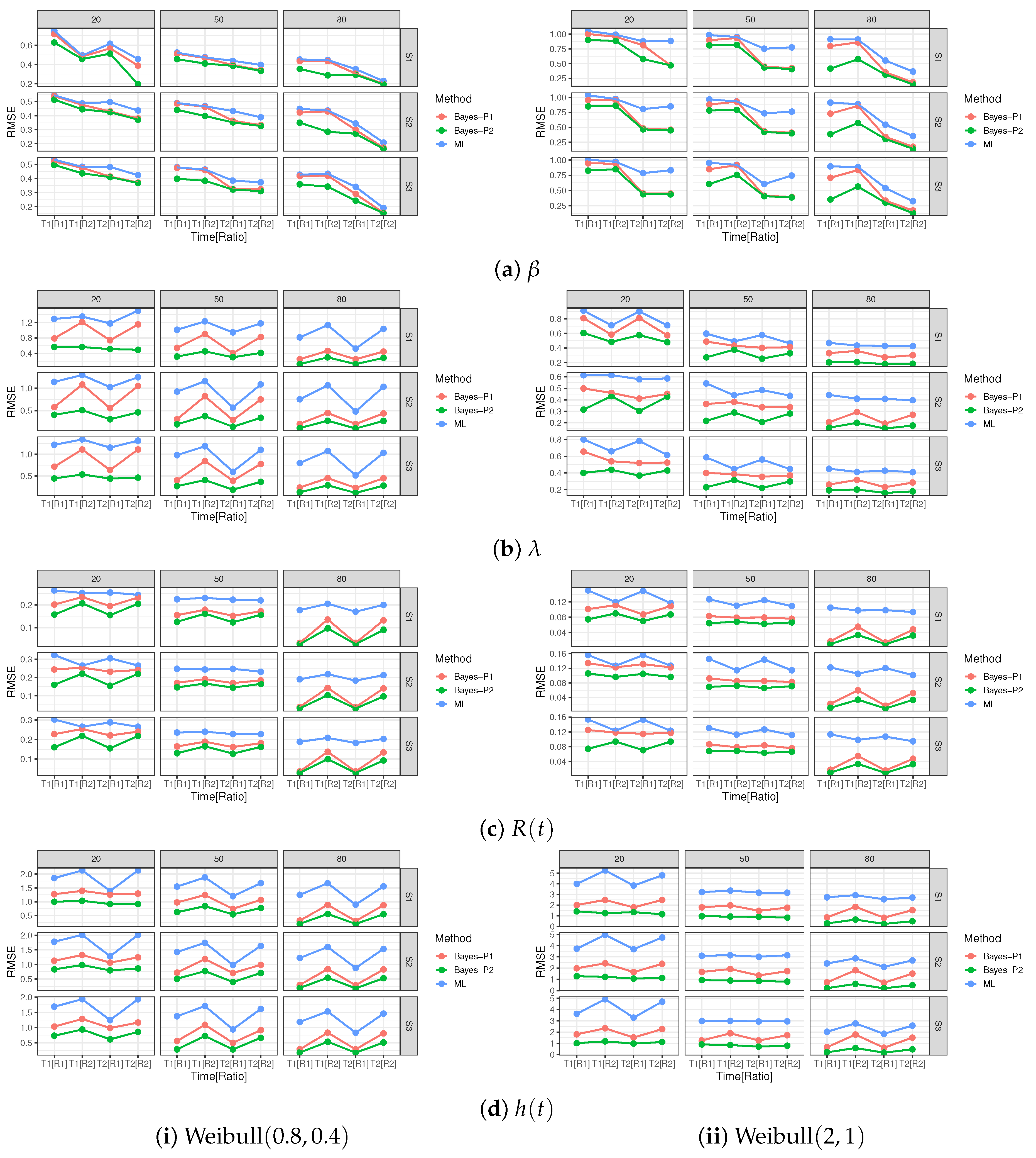
A simple representation of the simulation results for , , , and is depicted in Figure 6. In Table 4, Table 5, Table 6, Table 7, Table 8, Table 9, Table 10 and Table 11, we list the corresponding simulation findings of , , , and . To distinguish, in these tables, we referred to the specified threshold (for ) as Time-1[T1]:(0.5,1) and Time-2[T2]:(1,1.5) as well as the specified failure proportions () as Ratio-1[R1]:(0.4,0.5,0.6) and Ratio-2[R2]:(0.5,0.7,0.9). The following key findings can be presented, highlighting configurations that yield the lowest RMSEs, ARABs, and AILs, as well as the highest CPs:
Figure 6.
Plots illustrating the simulated RMSE results for , , , and .
Table 4.
The RMSE (1st Col.) and ARAB (2nd Col.) results of .
Table 5.
The RMSE (1st Col.) and ARAB (2nd Col.) results of .
Table 6.
The RMSE (1st Col.) and ARAB (2nd Col.) results of .
Table 7.
The RMSE (1st Col.) and ARAB (2nd Col.) results of .
Table 8.
The AIL (1st Col.) and CP (2nd Col.) results of .
Table 9.
The AIL (1st Col.) and CP (2nd Col.) results of .
Table 10.
The AIL (1st Col.) and CP (2nd Col.) results of .
Table 11.
The AIL (1st Col.) and CP (2nd Col.) results of .
- Both frequentist and Bayesian estimates of , , , and perform satisfactorily with low RMSEs, ARABs, and AILs, as well as high CPs.
- Increasing the complete size (n) or the effective sample sizes () improves the accuracy of all calculated estimates.
- For fixed n, reducing the total number of () significantly decreases RMSEs, ARABs, and AILs, as well as increases CPs.
- Higher threshold values ( for ) generally lead to more accurate and stable results.
- As (for ) grows, for both Weibull populations analyzed, it is noted that:
- –
- The RMSEs and ARABs of decreased, while those of , , and increased;
- –
- The AILs of and decreased, while those of and increased;
- –
- The CPs of and decreased, while those of and increased.
- Smaller values of tend to increase censoring severity and estimator variability, while larger values of yield behavior closer to C-T2 plan. These findings highlight the role of failure-proportion thresholds as tuning parameters controlling the balance between information retention and testing cost.
- As Weibull increases, it is noted that:
- –
- The RMSEs and ARABs of and decreased, while those of and increased;
- –
- The AILs of , , and increased, while those of decreased;
- –
- The CPs of increased while those of , , and decreased.
- As (for ) grows, the total of censoring items narrows down; thus, the calculated estimates become efficient. This is due to the number of the higher effective sample size (m) increasing.
- Bayesian estimates of , , , and using the MH–Gibbs algorithm outperform classical estimates.
- Comparing the proposed interval approaches, we noted that:
- –
- Comparing the credible intervals, the estimated bounds of , , , and from the HPD method behaved more satisfactorily than those developed from the BCI method.
- –
- Comparing the asymptotic intervals, the estimated bounds of , , , and from the NA-ACI method behaved more satisfactorily than NL-ACI for and , while the opposite was true for and .
- –
- The HPD intervals outperform all proposed intervals, including NA-ACI, NL-ACI, and BCI estimates, providing shorter AILs and higher CPs.
- –
- Across most given setups, the calculated CPs of all interval results for , , , or closely align with the nominal 95% confidence level.
- Comparing the proposed censoring designs Dß for listed in Table 3, we noted that:
- –
- The results developed by D3 (right censoring) are more accurate for and ;
- –
- The results developed by D2 (middle censoring) are more accurate for ;
- –
- The results developed by D1 (left censoring) are more accurate for ;
- Prior-1 denotes a diffuse prior with a higher variance, showing little prior knowledge, whereas Prior-2 corresponds to a focused prior.
- Posterior mean estimates are comparable under both Prior-1 and Prior-2; however, Prior-2 results in reduced posterior variability, tighter HPD intervals, and higher CPs.
- In conclusion, for analyzing component lifetimes from the Weibull population as a representative case, the proposed censoring mechanism, which incorporates failure proportions across all censoring stages, performs accurately and efficiently.
6. Multidisciplinary Data Analysis
To highlight the practical utility of the introduced censoring plan and the associated estimation procedures, and to highlight their adaptability across diverse real-world analytical contexts, this section presents five empirical applications from clinical, physics, chemistry, geology, and petroleum engineering (see Table S1). Below, we provide a concise overview of all datasets investigated, focusing on their scientific background, as follows:
- Clinical Application: Hypertension is a major public health concern because it progresses silently yet significantly increases the risk of serious cardiovascular conditions such as stroke, heart attack, and kidney disease, and its prevention and control are essential. The proposed censoring is illustrated using a clinical dataset (denoted as S[1]) containing observed survival times, recorded in years as the duration until the development of hypertension, for 119 patients treated at Bolgatanga Regional Hospital in Ghana’s Upper East Region (see Zamanah et al. [13]).
- Physics Application: Fracture toughness, measured in MPa·m1/2, is a physical property that characterizes a material’s resistance to crack initiation and propagation under stress. In the case of alumina (Al2O3), a widely used advanced ceramic, understanding its fracture toughness is pivotal for exploring the material’s intrinsic mechanical behavior, including atomic bonding strength, microstructural effects, and energy dissipation mechanisms at crack tips. This application analyzes a physical dataset (say, S[2]) that represents 119 observations on the fracture toughness from Alumina; see Ramadan et al. [14].
- Chemistry Application: Vinyl chloride, a synthetic organochloride gas first identified by Justus von Liebig and Henri Victor Regnault in 1835. As a colorless, highly flammable chemical with a distinctive sweet odor and a well-established classification as a human carcinogen, its presence in environmental systems warrants meticulous quantitative assessment. This application analyzes a chemical dataset (say, S[3]) that provides 34 observations collected from clean up-gradient monitoring wells; see Elshahhat et al. [15].
- Geology Application: The U.S. Geological Survey (USGS) stream-gaging network follows uniform protocols; the resulting time series are unbiased and comparable across years and across sites. It provides a robust baseline against which natural variability, extreme events (e.g., droughts or floods), and long-term changes in hydrologic regime can be assessed. This application analyzes a geological dataset (say, S[4]) that provides stream flow records during a 35-year series (1936–1970) of 1 April–31 August flow volumes (in 1000 acre-feet) at USGS gaging station no. 9-3425, which constitute a foundational resource for hydrologic research; see Nawaz et al. [16].
- Petroleum Application: Global oil reserves constitute a key determinant of economic resilience, geopolitical strategy, and long-term energy planning. This study analyzes a global oil dataset (say, S[5]) containing the largest oil reserves (in thousand million barrels) in 2020 for the top 20 countries, providing a rich empirical basis for modeling heterogeneity in resource distribution across diverse geographical and political contexts; see Alotaibi et al. [17].
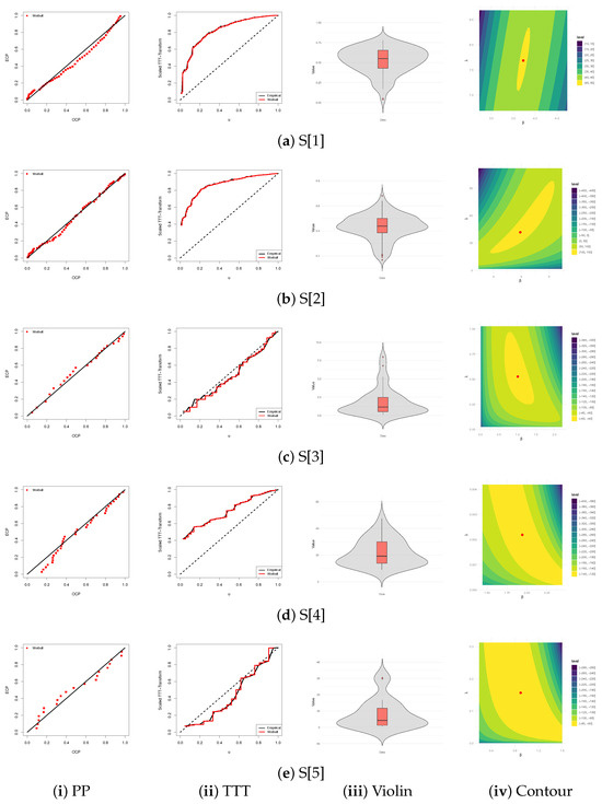
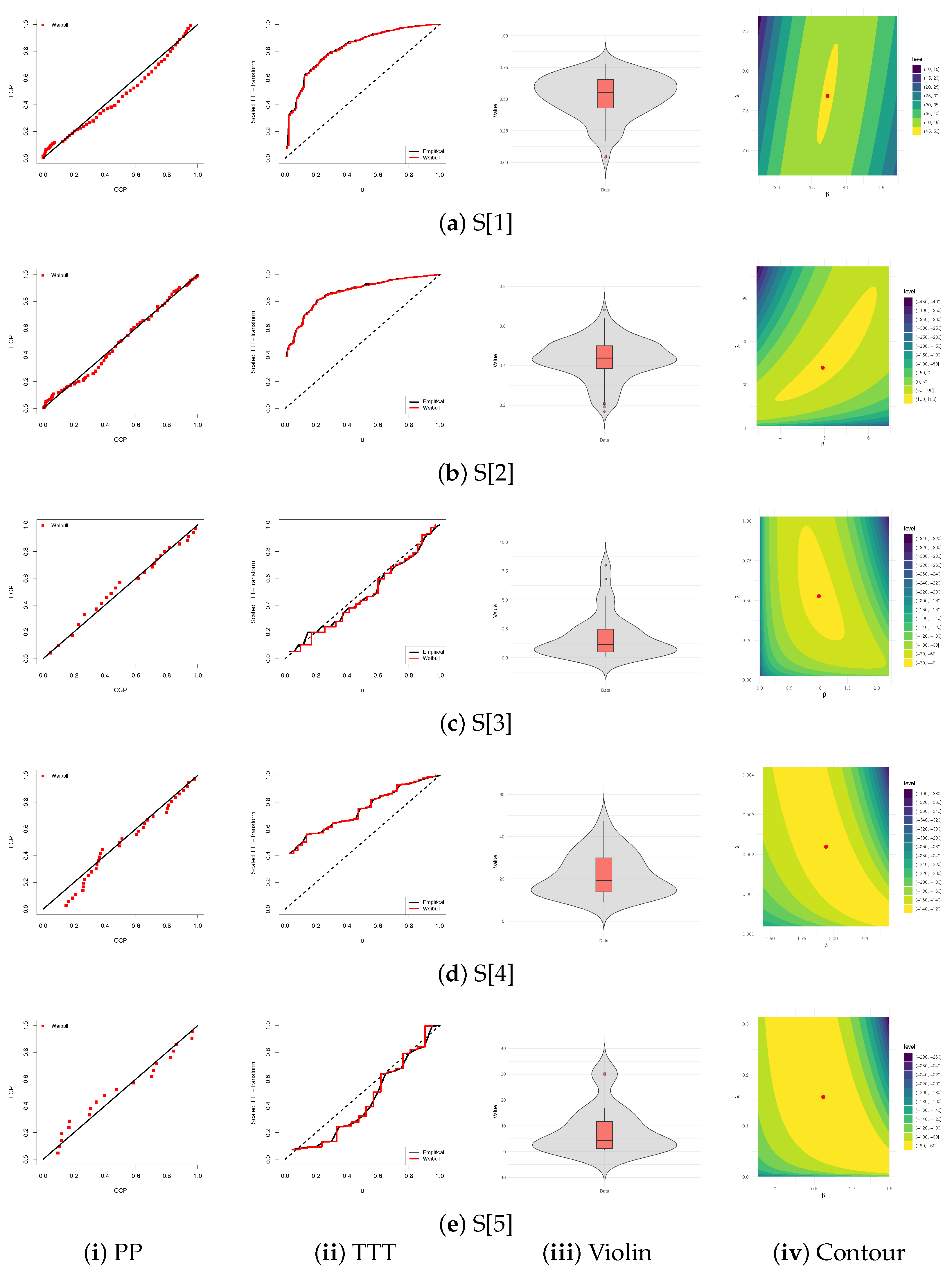
Datasets S[i] (), summarized in Table S1, are employed to assess the adequacy of the Weibull model under each scientific setting considered. For this purpose, the MLEs and their standard-errors (Std.Es) are used to compute the Kolmogorov–Smirnov () statistic and the associated p-value, see Table 12. The same table also presents the interval widths (IWs) of the 95% NA-ACI and NL-ACI for and . All analyses are conducted in R (version 4.4.2) using the AdequacyModel package by Marinho et al. [18]. As a result, since all estimated p-values are exceed 5%, we conclude that the Weibull model fits satisfactorily all multidisciplinary datasets S[i] (for ) listed in Table 12. To visually validate the numerical fitting performance of the Weibull model relative to its competitors, Figure 7 presents several diagnostic plots, including: (i) probability–probability (PP) plots, (ii) scaled total time on test (TTT) transform plots, (iii) log-LF contours, and (iv) boxplot-overlaid violin plots. From Figure 7, it is evident that:
Table 12.
Fitting summary of the Weibull model from multidisciplinary datasets.
Figure 7.
Fitting diagrams of the Weibull model from multidisciplinary datasets.
- The subplots in Figure 7 (i) show a good fit from S[i] (for ), with S[1] closely following the theoretical line, whereas S[i] (for ) show mild to moderate tail deviations, exhibiting an adequate fit;
- The subplots in Figure 7 (ii) reveal that the given datasets S[i] (for ) provide increasing failure rates, while those of S[i] (for ) provide decreasing failure rates. All estimated TTT curves support and follow the theoretical Weibull failure rates;
- The subplots in Figure 7 (iii) reveal a clear transition from low variability to pronounced dispersion and heavy-tailed behavior across the samples. The violins corresponding to for exhibit tightly to moderately concentrated distributions around their medians, with only mild skewness and a limited number of lower-end outliers, indicating generally stable behavior. In contrast, the violins of S for display evident right skewness accompanied by noticeable upper-end outliers, reflecting increasing upper-tail variability and dispersion. Finally, the violin plot for S[5] shows the highest degree of heterogeneity, characterized by a very wide spread and extremely large values, emphasizing the presence of substantial dispersion and heavy-tailed behavior;
- The subplots in Figure 7 (iv) indicate that the surface is relatively flat around the optimum; consequently, the fitted estimates of and developed from S[i] (for ) exist and are unique. It reflects a good curvature of the likelihood and stable parameter precision.
Again, using S[i] (for ) reported in Table S1, based on several configurations (listed in Table 13) of the failure ratios , thresholds , total sample sizes n, objective failure sizes , and PC-T2 styles, different MP–GC–T2 samples are collected and reported in Table S2.
Table 13.
Censoring designs in multidisciplinary data analysis.
For each dataset gathered by S[i,A], S[i,B], and S[i,C] (for ) designs, the likelihood point estimates (along with 95% NA-ACI/NL-ACI bounds) and MCMC estimates (along with 95% BCI/HPD bounds) of , , , and , are calculated. Specifically, to develop the estimation findings of R(t) and h(t), we assign t = 0.25 for S[i] (for i = 1, 2, 3), and 10 and 1 for S[i] (for i = 4, 5), respectively. By setting ℧ = 40,000, = 10,000, and = 30,000 in Algorithm 1, based on gamma impropers by equating to zero, the Bayes point and interval frameworks of , , , and are evaluated. In Table 14, Table 15, Table 16 and Table 17, the point and interval results along with their Std.E and IW values of , , , and are provided, respectively. Overall, the results in these tables demonstrate a consistent agreement between the classical (MLE-based ACI-NA and ACI-NL) and Bayesian (MCMC-based BCI and HPD) inferential frameworks of , , , and across all samples obtained by Table 13. While the MLEs of , , , and exhibit relatively small precision in comparison with the Bayesian estimates, they show noticeably higher posterior precision, reflected in much narrower BCI and HPD interval limits. This pattern highlights the stabilizing effect of the Bayesian approach, particularly under moderate sample sizes or higher parameter variability. Reliability and hazard estimates (, ) remain remarkably stable across samples, with Bayesian intervals consistently shorter and more concentrated. Overall, the comparative evidence indicates that Bayesian MCMC yields more precise inference. In contrast, the estimated ACI bounds—especially under NL transformations—tend to be more conservative and sensitive to sample-to-sample fluctuations. As a summary, the results of , , , and reveal that the MCMC MH-based setup performs better than the others based on minimum Std.E and IW values.
Table 14.
Estimates of from five real scenarios.
Table 15.
Estimates of from five real scenarios.
Table 16.
Estimates of from five real scenarios.
Table 17.
Estimates of from five real scenarios.
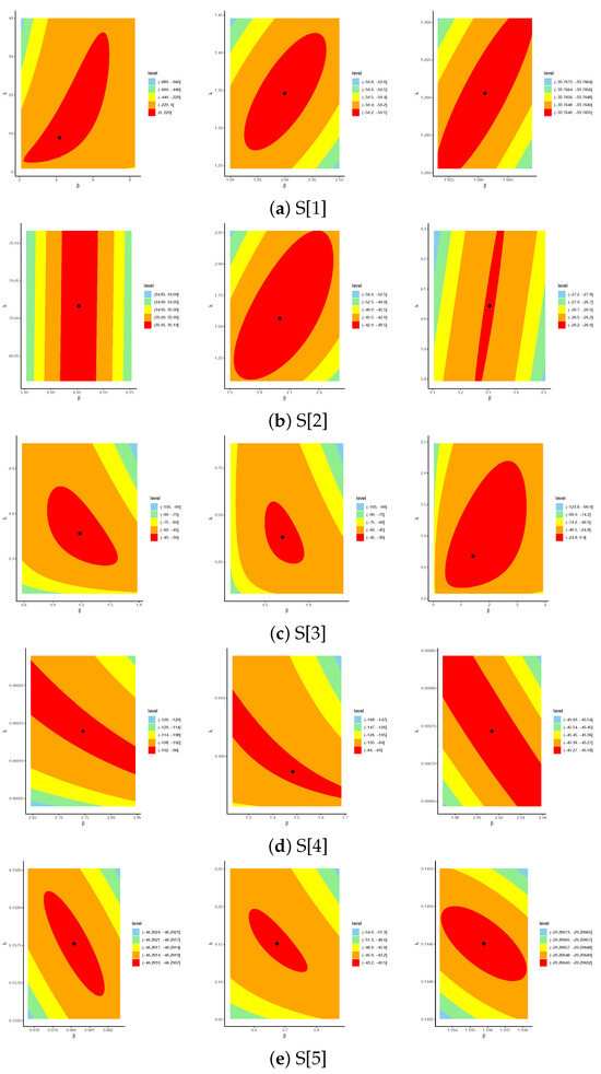
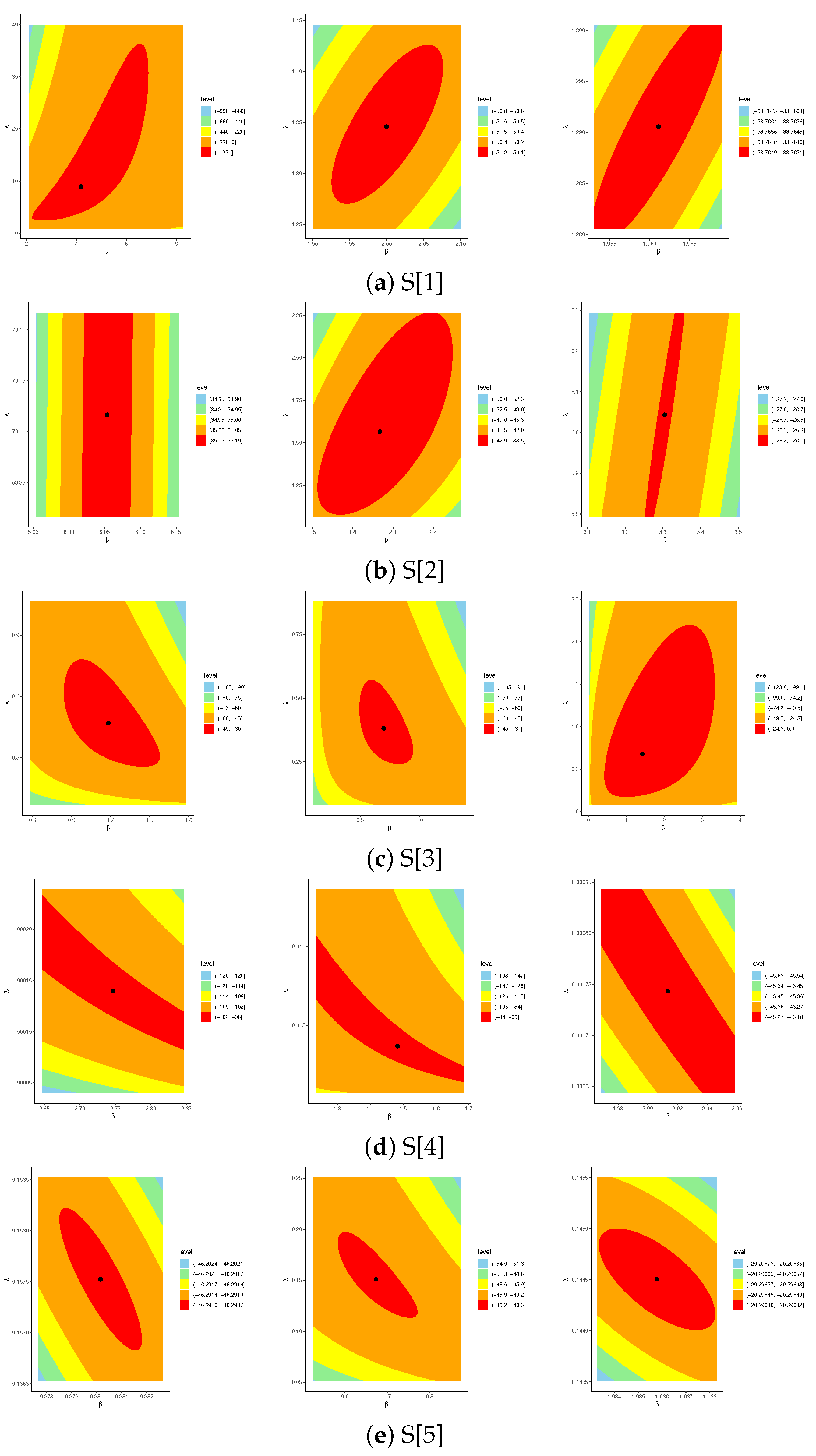
Figure 8 presents the log-LF contour diagrams for the Weibull() model, obtained using datasets gathered by S[i,A], S[i,B], and S[i,C] (for ). The contour patterns correspond well with the estimates reported in Table 14, Table 15, Table 16 and Table 17 and also verify the existence and uniqueness of the nonlinear likelihood solutions for , , , and . This offers strong empirical support for the stability of the proposed frequentist estimation approach. As a result, all facts displayed by the deep contours in Figure 8 show that the MLEs and existed and are unique, as well as support their theoretical findings developed in Corollary 2.
Figure 8.
Contours of Weibull parameters using S[i,A] (left), S[i,B] (middle), and S[i,C] (right) (for ) from five real scenarios.
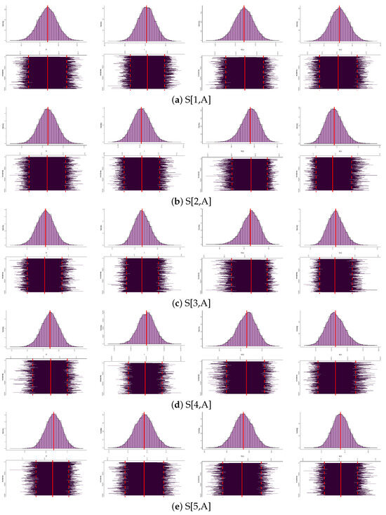
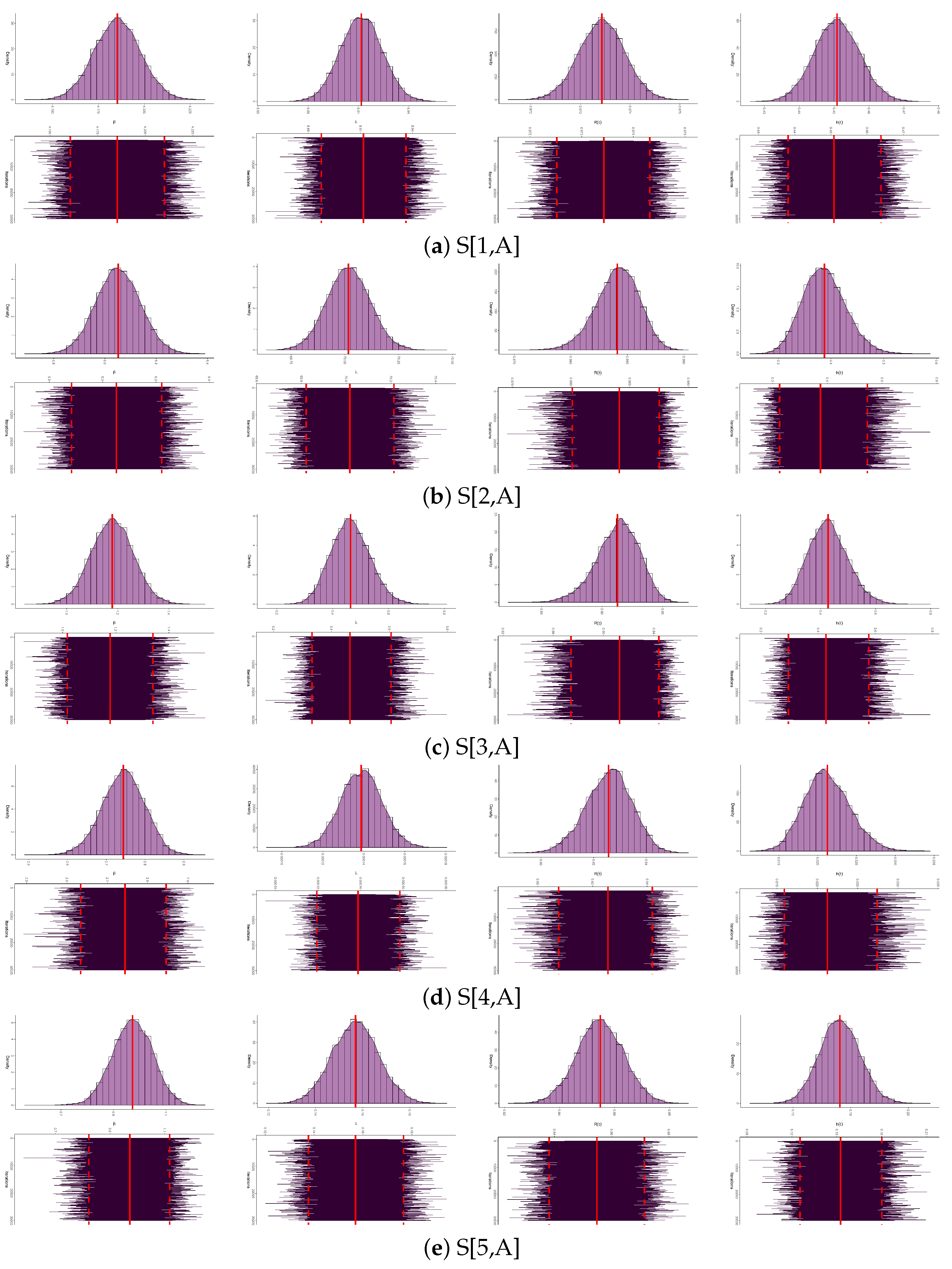
Trace plots and kernel density estimates are created for , , , and by employing S[i,A] (for ) to serve as representative cases to examine the distribution and convergence of 30,000 Markovian iterations of , , , and . The diagnostic findings in Figure 9 demonstrate good mixing and evident convergence of the MCMC chains. Furthermore, the marginal posterior distributions of the , , , and seem to be slightly symmetric.
Figure 9.
Convergence diagnostics of , , , and from five real scenarios.
7. Optimality Censoring Plans
In designing an experiment under the proposed framework, the experimenter must specify in advance the failure ratios , thresholds , total sample sizes n, objective failure sizes , and the PC-T2 . Since many censoring schemes can be constructed from these quantities, an important practical question is how to identify the censoring scheme that yields the most information about the model parameters. The search for an ‘optimal’ PC-T2 plan has gained considerable attention in the recent literature; see, for example, Lin et al. [19] and Mohammed et al. [20], and references cited therein.
For single-parameter models, variance-based measures are commonly used to assess optimality. However, for models involving multiple parameters, criteria based on the determinant or trace of the FIM (or its inverse) are generally preferred. Below, for evaluating PC-T2 designs beyond assigning the values of the failure ratios , thresholds , total sample sizes n, and objective failure sizes , we provide several roles:
- Role[1]:
- Role[2]:
- Role[3]:
- Role[4]:
Where denotes the log-(uth) quantile such as:
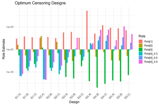
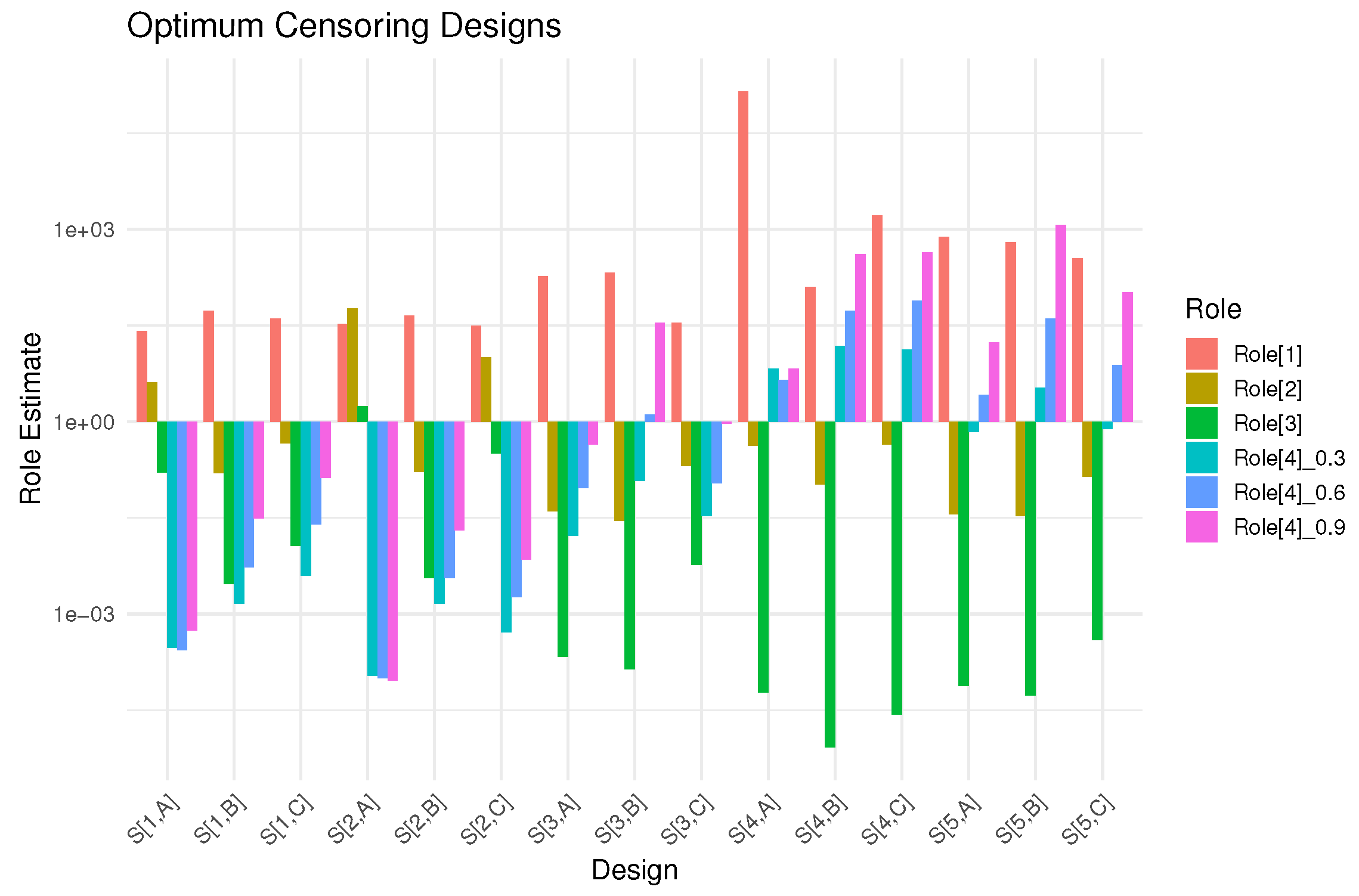
To clarify, the goal of Role[1] is to maximize the observed FIM data, while Role[i] (for ) aims to minimize both the determinant and trace of the VCM associated with the MLEs and . In contrast, Role[4] focuses on minimizing the variance of the log-(uth) quantile. From the five real-world scenarios proposed and in turn to examine the process of choosing an optimal PC-T2 technique, we estimate the proposed Role[i] (for ) based on S[i,A], S[i,B], and S[i,C] (for ) reported in Table S2; see Table 18. Subsequently, the optimal PC-T2 plan corresponds to achieving the lowest values for Role[i] (for ) and the highest value for R[1]. A simple visual representation of the fitted results mentioned in Table 2 is shown in Figure 10. The results, as shown in Table 18, demonstrate that:
Table 18.
Estimates of optimum roles from five real scenarios.
Figure 10.
Optimum estimates from five real scenarios.
- Using Role[4], the left-censoring (in S[1,A]), right-censoring (in S[i,C] for ), and middle-censoring (in S[4,A]) are the optimum;
- Using Role[i] for , the middle-censoring (in S[i,B] (for )) is the optimum;
- Using Role[1], the left-censoring (in S[i,A] (for )) is the optimum censoring compared to others.
Additionally, one of the most significant findings reported in Table 18 is that the proposed optimal censoring strategies, analyzed across five different real-world scenarios, support our recommended censoring strategies outlined in Section 5. This framework offers a systematic approach for comparing competing censoring designs and identifying the plan that yields the most informative and efficient inferential outcomes.
8. Conclusions and Future Research
The present study makes several significant methodological, computational, and practical contributions to the statistical examination of lifetime data under censoring constraints. First, it introduces the MP–GC–T2 scheme, a unified censoring structure that simultaneously incorporates multi-stage failure proportion regulation, progressive removals of surviving units, and two flexible temporal thresholds. This combination provides a level of adaptability not available in existing censoring plans. It also embeds, as special or limiting cases, numerous classical and modern censoring mechanisms—including C-T2, GC-T2, PC-T2, H-PC-T2, A-PC-T2, and IA-PC-T2—thus, offering a general framework within which all of these schemes can be compared, optimized, and operationalized. Second, the full MP–GC–T2’s likelihood is derived in a tractable analytic form for all possible stopping scenarios, enabling researchers to perform rigorous LF-based inference. Using this foundation, explicit MLEs for the scale parameter and profile-LF estimation for the shape parameter of the Weibull model are developed. Two asymptotic interval procedures (NA-based and NL-based) are further established for all parameters and reliability metrics, providing multiple practical tools for uncertainty quantification. Third, a Bayesian estimation framework is constructed using independent gamma priors, leading to closed-form conditional posterior distributions for the scale parameter and a non-standard posterior for the shape parameter. A hybrid MH–G sampling algorithm is proposed to efficiently sample from these posterior distributions. This algorithm is demonstrated to be computationally stable and capable of producing accurate MCMC, BCI, and HPD bounds for all quantities of interest. The HPD intervals, in particular, show strong performance in terms of coverage and precision. Fourth, the paper develops an extensive Monte Carlo simulation that comprehensively evaluates estimator bias, mean squared error, relative error, interval length, and coverage probability across a wide range of censoring configurations, thresholds, failure proportions, priors, and total sample sizes. These experiments confirm the strong inferential properties of the proposed estimators, the superiority of Bayesian methods in most scenarios, and the robustness of the MP–GC–T2 scheme even under heavy censoring. Fifth, the study introduces a comprehensive framework for optimal plan selection, enabling experimenters to identify progressive removal patterns and failure-proportion settings that minimize estimator variability and maximize interval performance under specified time and cost constraints. This contribution offers a practical decision-making tool for reliability engineers and applied statisticians responsible for designing efficient life-testing experiments. Finally, the utility and flexibility of the MP–GC–T2 design are demonstrated through five real-data applications drawn from diverse scientific domains—including clinical, chemical, geological, physical, and petroleum engineering. These examples show that the proposed scheme successfully adapts to various hazard behaviors, censoring severities and experimental constraints, reinforcing its broad applicability and practical relevance beyond a single discipline.
Although the present study provides a comprehensive methodological foundation, several promising directions remain open for future research:
- Extending the MP–GC–T2 framework to other lifetime distributions—such as the generalized gamma, log-logistic, inverse Gaussian, or exponentiated models—would increase applicability in biomedical, industrial, and environmental settings.
- Embedding the proposed censoring plan within accelerated life testing, proportional hazards, or frailty models would allow inference under complex covariate effects.
- Decision-theoretic, Bayesian, or utility-based optimization of , , and the progressive removal vector may yield more efficient experimental strategies, particularly for high-cost or destructive testing.
- Future work may develop robust estimators based on empirical likelihood, minimum divergence, or semi-parametric hazards to address model misspecification and heavy-tailed lifetime behavior.
- Expanding the interval analyses proposed by incorporating resampling-based processes into the suggested censoring setup. Utilizing bootstrap confidence intervals, including percentile and bias-corrected methods, can enhance finite-sample accuracy and offer an alternative estimate of inferential uncertainty.
- Incorporating Hamiltonian Monte Carlo, slice sampling, or variational Bayesian methods may improve convergence under heavy censoring. Diagnostic tools quantifying information contribution at each censoring stage could guide better removal patterns.
- Applying MP–GC–T2 to series, parallel, and mixed systems would enable inference at the subsystem or system level, supporting applications in aerospace, energy systems, and industrial engineering.
- Machine-learning or reinforcement-learning techniques may be used to determine optimal temporal thresholds and failure proportions based on real-time failure information.
Overall, the MP–GC–T2 scheme offers a unified and versatile censoring structure that effectively balances test duration, cost, and precision. Its flexibility, strong inferential properties, and broad applicability make it a valuable platform for further methodological development and interdisciplinary reliability research.
Supplementary Materials
The following supporting information can be downloaded at: https://www.mdpi.com/article/10.3390/math14050862/s1, Table S1: Failure times of multidisciplinary datasets; Table S2: Different MP–GC–T2 samples from multidisciplinary datasets.
Author Contributions
Methodology, H.S.M. and A.E.; Funding acquisition, H.S.M.; Software, A.E.; Resources, H.S.M.; Supervision, A.E.; Writing—original draft, H.S.M. and A.E.; Writing—review and editing, H.S.M. and A.E. All authors have read and agreed to the published version of the manuscript.
Funding
The authors extend their appreciation to the Deanship of Scientific Research and Libraries in Princess Nourah bint Abdulrahman University for funding this research work through the Supporting Publication in Top-Impact Journals Initiative (SPTIF-2026).
Data Availability Statement
The authors confirm that the data supporting the findings of this study are available within the article.
Conflicts of Interest
The authors declare no conflicts of interest.
Appendix A. Derivation of the Likelihood Function
This appendix derives the likelihood function in Equation (1) conditional on the realized censoring configuration. Specifically, the derivation is carried out given the terminal number of observed failures , corresponding to Case–i (), and the predetermined progressive removal vector .
Proof.
Define
as the final stage at which progressive removals are implemented. The associated removal scheme is , where each is fixed in advance.
At time zero, all n units are placed on test. For , let denote the number of units at risk immediately prior to the ith observed failure. Then
which reflects the removal of failed units together with the cumulative progressive withdrawals up to stage . In particular, no removals occur after stage B.
Given , the conditional density contribution of observing a failure at time is
The product depends only on and is therefore free of ; it may be absorbed into a normalizing constant.
Progressive withdrawals occur only for . Immediately after the ith failure, exactly surviving units are removed. Each such unit must have survived beyond , contributing a factor . Hence, the joint contribution of all progressive removalsis
The experiment terminates at . At that time, the remaining
units are right-censored and contribute
Combining (A1)–(A3), the conditional likelihood function takes the form
where
is a combinatorial factor independent of .
Eliminating this constant yields the likelihood kernel reported in Equation (1). □
References
- Long, Q.; Jiang, D. Parameter estimation and reliability analysis of Burr XII distribution under generalized type-II censoring. Phys. Scr. 2025, 100, 095240. [Google Scholar] [CrossRef] [Scilit]
- Balakrishnan, N.; Cramer, E. The Art of Progressive Censoring. Statistics for Industry and Technology; Springer: New York, NY, USA; Birkhäuser: New York, NY, USA, 2014. [Google Scholar]
- Kundu, D.; Joarder, A. Analysis of Type-II progressively hybrid censored data. Comput. Stat. Data Anal. 2006, 50, 2509–2528. [Google Scholar] [CrossRef] [Scilit]
- Ng, H.K.T.; Kundu, D.; Chan, P.S. Statistical analysis of exponential lifetimes under an adaptive Type-II progressive censoring scheme. Nav. Res. Logist. 2009, 56, 687–698. [Google Scholar] [CrossRef] [Scilit]
- Yan, W.; Li, P.; Yu, Y. Statistical inference for the reliability of Burr-XII distribution under improved adaptive Type-II progressive censoring. Appl. Math. Model. 2021, 95, 38–52. [Google Scholar] [CrossRef] [Scilit]
- Bain, L.J.; Engelhardt, M. Statistical Analysis of Reliability and Life-Testing Models, 2nd ed.; Marcel Dekker: New York, NY, USA, 1991. [Google Scholar]
- Greene, W.H. Econometric Analysis, 4th ed.; Prentice-Hall: New York, NY, USA, 2000. [Google Scholar]
- Oehlert, G.W. A note on the delta method. Am. Stat. 1992, 46, 27–29. [Google Scholar] [CrossRef] [Scilit]
- Meeker, W.Q.; Escobar, L.A. Statistical Methods for Reliability Data; John Wiley and Sons: New York, NY, USA, 1998. [Google Scholar]
- Kundu, D. Bayesian inference and life testing plan for the Weibull distribution in presence of progressive censoring. Technometrics 2008, 50, 144–154. [Google Scholar] [CrossRef] [Scilit]
- Henningsen, A.; Toomet, O. maxLik: A package for maximum likelihood estimation in R. Comput. Stat. 2011, 26, 443–458. [Google Scholar] [CrossRef] [Scilit]
- Plummer, M.; Best, N.; Cowles, K.; Vines, K. coda: Convergence diagnosis and output analysis for MCMC. R News 2006, 6, 7–11. [Google Scholar]
- Zamanah, E.; Nasiru, S.; Luguterah, A. Harmonic Mixture Weibull-G Family of Distributions: Properties, Regression and Applications to Medical Data. Comput. Math. Methods 2022, 2022, 2836545. [Google Scholar] [CrossRef] [Scilit]
- Ramadan, D.A.; Tashkandy, Y.A.; Bakr, M.E.; Balogun, O.S.; Hasaballah, M.M. Analysis of Marshall–Olkin extended Gumbel type-II distribution under progressive type-II censoring with applications. AIP Adv. 2024, 14, 055137. [Google Scholar] [CrossRef] [Scilit]
- Elshahhat, A.; Abo-Kasem, O.E.; Mohammed, H.S. Statistical analysis of Type-II generalized progressively hybrid alpha-PIE censored data and applications in electronic tubes and vinyl chloride. Axioms 2023, 12, 601. [Google Scholar] [CrossRef] [Scilit]
- Nawaz, T.; Hussain, S.; Ahmad, T.; Naz, F.; Abid, M. Kumaraswamy generalized Kappa distribution with application to stream flow data. J. King Saud Univ.-Sci. 2020, 32, 172–182. [Google Scholar] [CrossRef] [Scilit]
- Alotaibi, R.; Rezk, H.; Elshahhat, A. Efficient Analysis of the Gompertz–Makeham Theory in Unitary Mode and Its Applications in Petroleum and Mechanical Engineering. Axioms 2025, 14, 775. [Google Scholar] [CrossRef] [Scilit]
- Marinho, P.R.D.; Silva, R.B.; Bourguignon, M.; Cordeiro, G.M.; Nadarajah, S. AdequacyModel: An R package for probability distributions and general purpose optimization. PLoS ONE 2019, 14, e0221487. [Google Scholar] [CrossRef] [Scilit] [PubMed]
- Lin, C.T.; Chen, Y.C.; Yeh, T.C.; Ng, H.K.T. Statistical inference and optimum life-testing plans with joint progressively type-II censoring scheme. Qual. Technol. Quant. Manag. 2023, 20, 279–306. [Google Scholar] [CrossRef] [Scilit]
- Mohammed, H.S.; Abo-Kasem, O.E.; Elshahhat, A. Analysis and optimum removals of unit-Weibull data from progressive first-failure censoring and its modeling in chemistry and physics. J. Stat. Comput. Simul. 2025, 95, 3970–4002. [Google Scholar] [CrossRef] [Scilit]

Disclaimer/Publisher’s Note: The statements, opinions and data contained in all publications are solely those of the individual author(s) and contributor(s) and not of MDPI and/or the editor(s). MDPI and/or the editor(s) disclaim responsibility for any injury to people or property resulting from any ideas, methods, instructions or products referred to in the content. |
© 2026 by the authors. Licensee MDPI, Basel, Switzerland. This article is an open access article distributed under the terms and conditions of the Creative Commons Attribution (CC BY) license.