Recursive Least-Squares Algorithm Based on a Fourth-Order Tensor Decomposition for Acoustic Echo Cancellation

Abstract

Adaptive filtering algorithms based on tensor decomposition represent appealing choices for system identification problems, especially when dealing with the estimation of long-length impulse responses, like in acoustic echo cancellation. The topic has recently been addressed in the literature, showing that the gain (compared to the conventional approach) is twofold in terms of both better performance and lower complexity. The main idea is that a system identification problem with a large parameter space (i.e., a long-length filter) is reformulated based on a group of shorter filters, while their coefficients are combined using the Kronecker product. Nevertheless, one of the main challenges is related to handling the tensor rank, which is particularly addressed for each specific decomposition order. Previous solutions have been designed for second-order (matrix case) and third-order tensorial decompositions. In this paper, we develop a recursive least-squares adaptive filtering algorithm that exploits a fourth-order tensor decomposition, aiming for further performance improvements compared to the existing solutions. In this framework, the influence of the decomposition setup is investigated, which is also related to the main parameters of the algorithm, i.e., the forgetting factors. Simulations performed in the context of acoustic echo cancellation support the theoretical findings and indicate the good performance of the proposed algorithm.

1. Introduction

Adaptive filters represent popular and powerful signal processing tools, being involved in a wide range of applications, especially in those requiring real-time capabilities and nonstationary operating conditions [1,2,3]. The control unit for such a filter is the adaptive algorithm, which implements an optimization process by minimizing a cost function that depends on the so-called error signal. This error is defined as the difference between a reference (or desired) signal and the output of the adaptive filter. As a result, following the optimization criterion, the coefficients of the adaptive filter are iteratively updated for this purpose. Nevertheless, while the functionality principle can be straightforwardly formulated, there are inherent challenges related to real-world applications in which adaptive filters are involved [4].

There are several performance criteria used to assess the overall behavior of an adaptive filter. First, the convergence rate is a major asset since it indicates how “fast” (in terms of number of iterations) the adaptive algorithm reaches a steady-state solution. On the other hand, the accuracy (or misadjustment) of this result is also important, showing how “close” to the optimal solution it is. Unfortunately, these two performance criteria are conflicting requirements, leading to the well-known compromise between “fast” and “accurate” [1,2,3]. Moreover, because adaptive filters are designed to operate in time-varying conditions, the tracking capabilities are extremely important since the algorithm should recover after any changes related to the environment. Finally, the computational complexity of the adaptive algorithm (i.e., the number of arithmetic operations per iteration) represents a mandatory practical issue to be considered, especially when real-time features are required. All these performance criteria are highly influenced by the length of the adaptive filter (or its parameter space), which is basically related to the number of filter coefficients to be updated. In addition to higher computational complexity, a long-length adaptive filter is characterized by a slower convergence rate and tracking capabilities, while the accuracy of its solution is also reduced. Detailed theoretical proofs regarding the influence of filter length on these performance criteria of adaptive algorithms can be found in fundamental works [1,2,3].

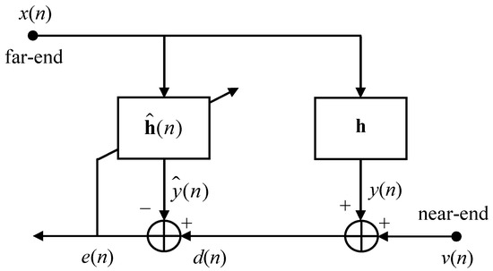
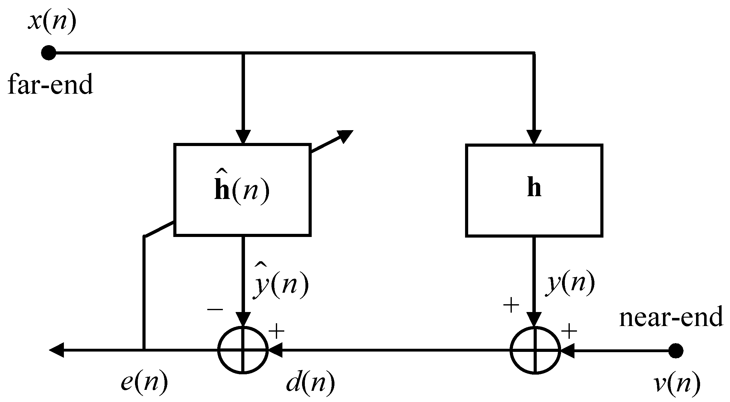
Long-length adaptive filters are frequently involved in many important applications, acoustic echo cancellation (AEC) being among the most popular ones [5]. This application can be formulated as an interesting combination between two adaptive filtering configurations [1,2,3]. First, it can be interpreted as a system identification problem since the main goal of the adaptive filter is to model/estimate the echo path, which inherently results due to the acoustic coupling between the loudspeaker and the microphone of the communication device, especially when operating in “hands-free” mode. Second, the AEC application also represents an interference cancellation problem, where the main goal is to remove the unwanted acoustic echo that corrupts the microphone signal. Figure 1 shows the basic scheme of the AEC configuration, where $x\left(n\right)$ denotes the input signal (also known as the far-end) at the discrete-time index n, while $d\left(n\right)$ is the microphone signal (i.e., the reference/desired signal), which consists of the acoustic echo, $y\left(n\right)$, and the near-end signal, $v\left(n\right)$. The impulse response of the acoustic echo path is denoted by $\mathbf{h}$, which is a column vector with L coefficients. The adaptive filter is characterized by the impulse response $\widehat{\mathbf{h}}\left(n\right)$, aiming to provide an estimate of $\mathbf{h}$ under the control of the error signal, $e\left(n\right)$; as a result, $\widehat{y}\left(n\right)$ represents a replica of the echo, which is subtracted from the microphone signal. It is assumed that the length of $\widehat{\mathbf{h}}\left(n\right)$ is also L, so the accuracy of the solution can be evaluated based on the so-called misalignment (or system mismatch) [5], which is defined as $∥\mathbf{h}-\widehat{\mathbf{h}}\left(n\right)∥$, where $∥·∥$ denotes the Euclidean norm.

Figure 1. Basic scheme for acoustic echo cancellation (as a system identification problem).

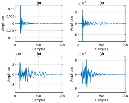
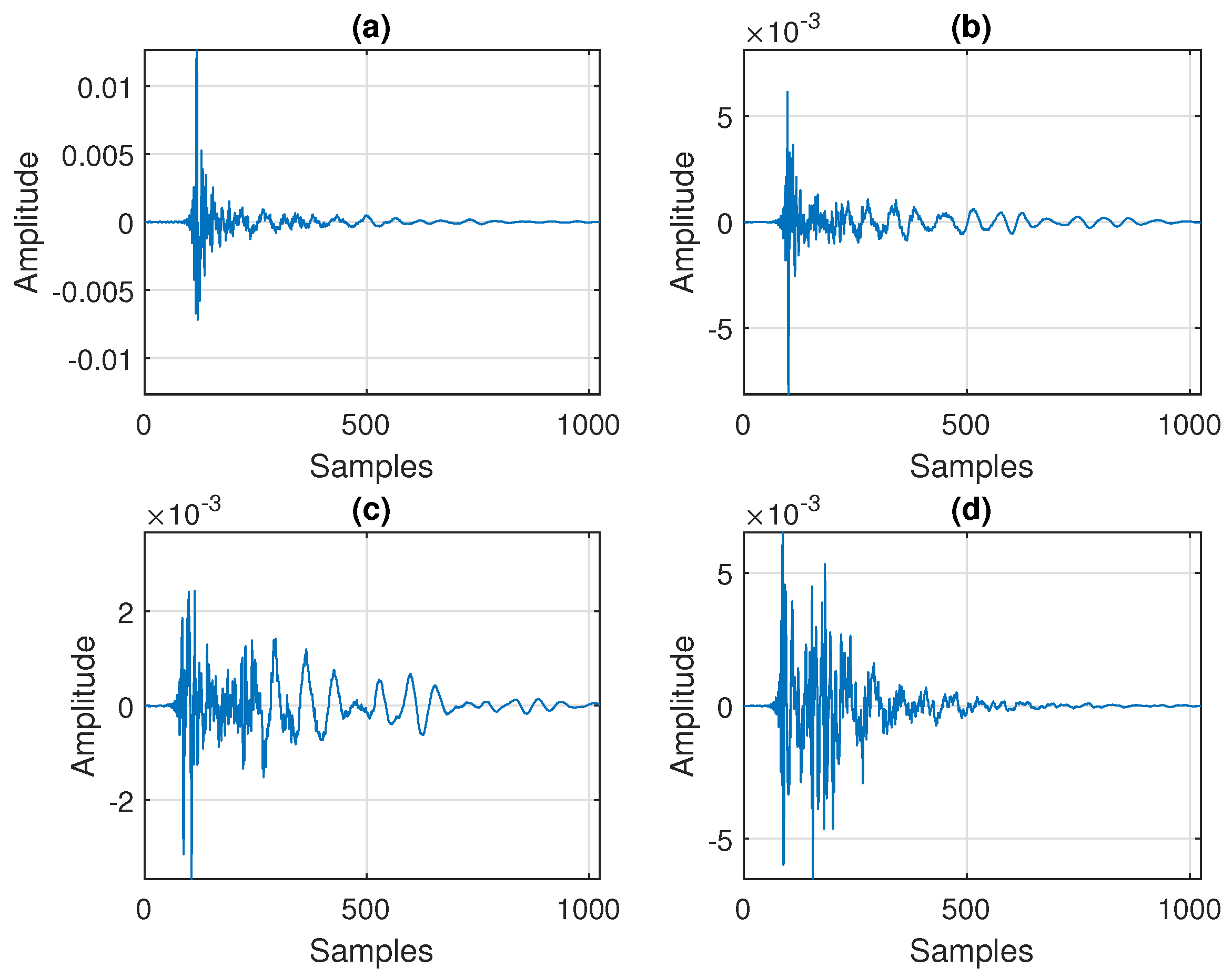
The acoustic echo paths are characterized by very long impulse responses, which can be of the order of thousands of coefficients [5]. Figure 2 shows four typical acoustic impulse responses (AIRs) with different reverberation times ($T_{60}$), each one of length $L=1024$, which are measured using a sampling rate of 8 kHz. Depending on the dimensions of the room and the reflecting surfaces, the AIR length can be even longer. Consequently, long-length adaptive filters should also be used to cope with such large values of L, thus facing inherent challenges related to convergence rate, tracking, accuracy, and the computational complexity of the algorithm.

Figure 2. Typical acoustic impulse responses ($\mathbf{h}$) of length $L=1024$ (using a sampling rate of 8 kHz), with different reverberation times: (a) $T_{60}=0.241$ s, (b) $T_{60}=0.212$ s, (c) $T_{60}=0.180$ s, and (d) $T_{60}=0.145$ s.

Targeting a high convergence rate, the recursive least-squares (RLS) adaptive filtering algorithm [1,2,3] represents an appealing choice. This algorithm relies on the least-squares optimization criterion and is recognized as one of the most useful solutions. However, the computational complexity of the conventional RLS algorithm is proportional to the square of the filter length, which poses significant implementation challenges for large values of L. Several computationally efficient versions are available in the literature, which are usually referred to as “fast” RLS algorithms [6,7,8,9,10,11]. Nevertheless, these algorithms still handle a long-length adaptive filter, thus raising important challenges related to the tracking capabilities and accuracy of the resulting estimate.

The solution presented in this paper relies on a different approach for large system identification problems, which considers a “decomposition” of the impulse response such that the final (global) estimate is obtained via a combination of shorter adaptive filters via the Kronecker product [12]. The main idea can be formulated using tensor-based signal processing techniques, which can be found in many important frameworks and applications [13,14,15,16,17,18,19,20,21,22,23,24,25]. In other words, the vector $\mathbf{h}$ corresponding to the impulse response of the system is reshaped into the form of a tensor such that the parameter space can be reduced by manipulating the tensor’s components and exploiting its low-rank features [26,27,28,29]. For example, the RLS-type algorithm developed in [27] considers the second-order case, where the impulse response of length $L=L_1{L}_2$ (with $L_1\ge L_2$) is reshaped as a matrix of size $L_1\times L_2$ with the (approximated) rank $R<L_2$ [30,31]. As consequence, the resulting algorithm combines the solutions provided by two shorter adaptive filters of lengths $R{L}_1$ and $R{L}_2$. Since the low-rank features of the impulse responses fit very well for echo cancellation scenarios [26], the gain is twofold in terms of both performance and complexity. In [29], an RLS-based solution was designed in a third-order tensor decomposition framework, considering the factorization $L=L_{11}^{\prime }{L}_{12}^{\prime }{L}_2^{\prime }$, with $L_{11}^{\prime }\ge L_{12}^{\prime }$ and $L_{11}^{\prime }{L}_{12}^{\prime }\gg L_2^{\prime }$. By efficiently manipulating the third-order tensor decomposition, in order to avoid the sensitive approximation of the tensor rank [32,33], the global estimate of the impulse response is obtained by combining the solutions provided by three shorter adaptive filters of lengths ${L_2^{\prime }}^2$, $M{L}_{11}^{\prime }{L}_2^{\prime }$, and $M{L}_{12}^{\prime }{L}_2^{\prime }$, with $M<L_{12}^{\prime }$, outperforming the algorithm from [27]. Here, M represents the rank of a matrix that emerges during the specific decomposition [28,29], which is more advantageous instead of directly manipulating the tensor rank.

These decomposition-based techniques lead to appealing performance in different frameworks [34,35,36,37,38,39,40,41,42,43,44,45], including several applications related to the acoustic environment. Nevertheless, the RLS-type algorithms from [27,29] fit very well for network echo cancellation scenarios [46] when using small values of R and M, respectively, while these values should be increased for AEC applications. In this context, targeting a more efficient solution, the decomposition order could be increased while still aiming to avoid the direct approximation of the tensor rank, as outlined before. To this purpose, we follow a fourth-order decomposition, which was recently developed in the framework of the Wiener filter [47]. However, despite the Wiener filter being a reliable theoretical benchmark, it is not suitable for time-varying environments and nonstationary conditions, as is the case in AEC. Consequently, in this paper, we propose an RLS algorithm based on a fourth-order tensor (FOT) decomposition of the impulse response.

Summarizing, the general framework of our development is a system identification problem associated with the AEC application, targeting the estimation of the AIR corresponding to the echo path, as explained previously (Figure 1). In this context, since AIRs are usually modeled as long-length adaptive filters (as shown in Figure 2), the tensor-based decomposition technique represents an efficient approach. The existing solutions that exploit second-order and third-order decompositions fit very well for very sparse systems (like in network echo cancellation), while the values of their specific decomposition parameters should be increased for AEC, which could further raise computational complexity issues. Therefore, we aim to develop an RLS algorithm based on FOT decomposition (namely RLS-FOT) that is more suitable for AEC. Thus, the main contributions of the paper are

• the theoretical development of the RLS-FOT algorithm;
• the analysis of its decomposition parameters from a practical perspective;
• the analysis of the computational complexity of the proposed algorithm;
• the motivated choice of its convergence parameters, i.e., the forgetting factors.

The remainder of this paper is organized as follows. Next, Section 2 presents the background of the FOT-based decomposition. Then, the proposed RLS-type algorithm based on FOT is designed in Section 3. Its performance is assessed in the experimental framework of AEC based on a set of simulation results presented in Section 4. Finally, the conclusions and perspectives are discussed in Section 5.

2. Fourth-Order Tensor Decomposition

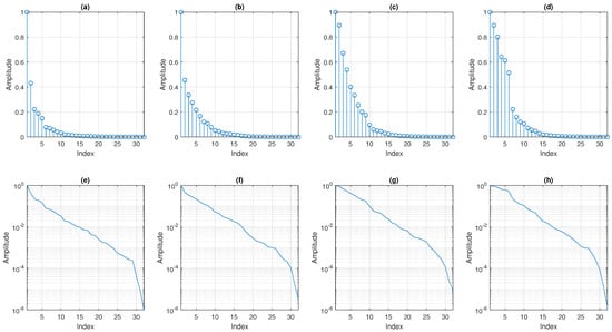
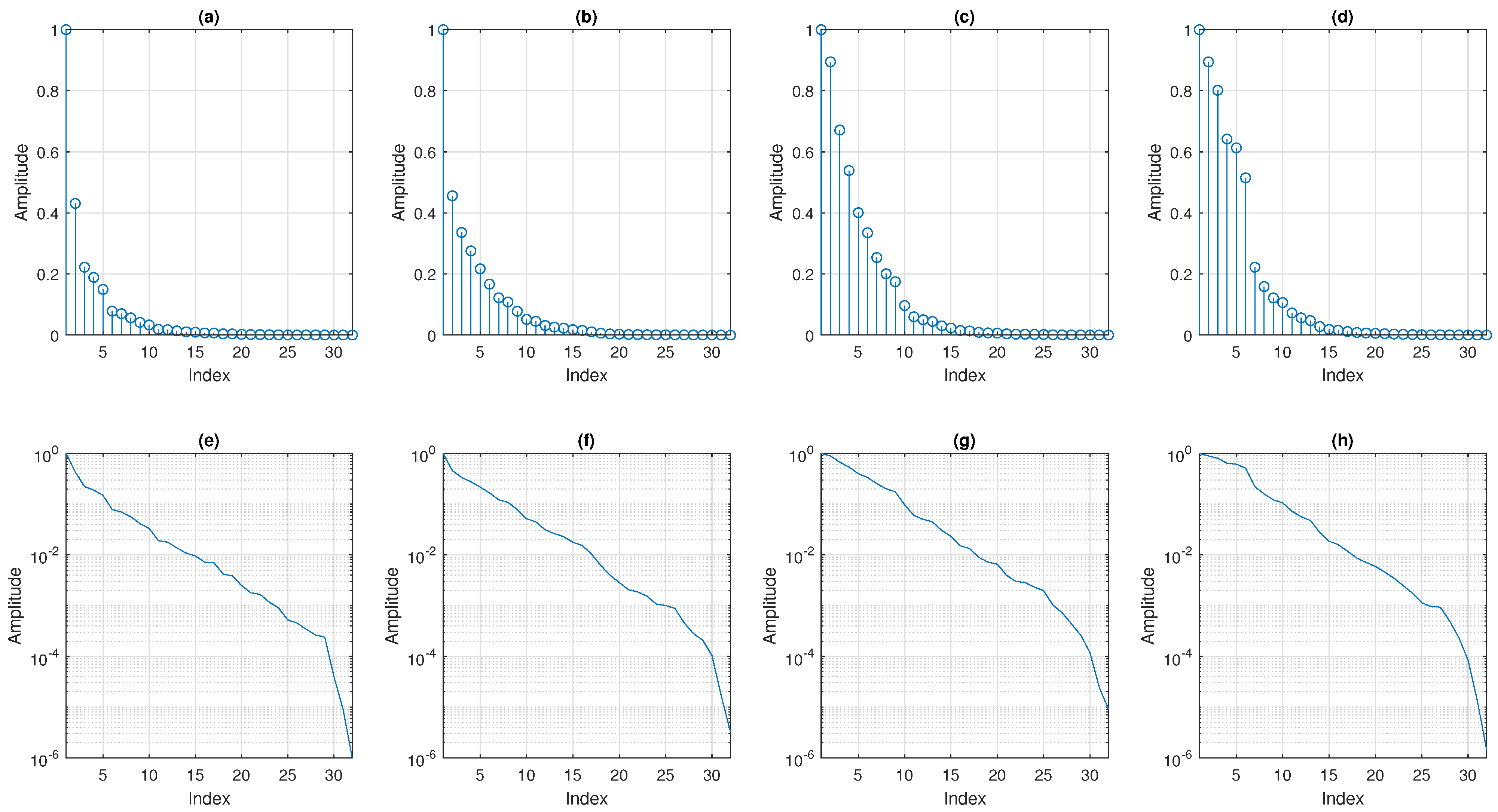
The basic scheme of AEC depicted in Figure 1 can be generally related to a linear system identification problem, in the framework of a single-input single-output (SISO) scenario. The unknown impulse response, $\mathbf{h}$, should be estimated using an adaptive filter. However, the AIR of the echo path has some specific features that can be exploited for a more efficient identification. As illustrated in Figure 2, the AIRs are sparse in nature, having many coefficients with small values (or even zero) [48]. More recently, this sparseness feature was also related to the low-rank property of such impulse responses [26]. This can be assessed by reshaping the impulse response ($\mathbf{h}$) of length $L=L_1{L}_2$ (with $L_1\ge L_2$) as an $L_1\times L_2$ matrix, $\mathbf{H}$, whose rank is $R<L_2$ [30,31]. For example, in the case of the AIRs from Figure 2, the factorization of $L=1024$ can be performed using $L_1=L_2=32$. Under these circumstances, the singular values of the resulting matrices $\mathbf{H}$ are depicted in Figure 3 using both linear and logarithmic scales. For each case, these values are normalized with respect to the maximum one for a proper comparison. As a visual indicator, it can be noticed that these values decrease to zero fast enough such that a reliable approximation of the rank of $\mathbf{H}$ could be around $L_2/2$. This can also be supported using appropriate thresholds, e.g., $0.01$ at linear scale or ${10}^{-2}$ at logarithmic scale.

Figure 3. Singular values (normalized with respect to the maximum one) of the matrices $\mathbf{H}$ (of size $32\times 32$) for the corresponding AIRs $\mathbf{h}$ (of length $L=1024$) from Figure 2. (a–d) Linear representations and (e–h) log-scale representations.

The identification of the AIRs using the decomposition-based approach relies on the low-rank property of these impulse responses. This is the main idea behind this technique, as outlined in one of the initial works on this subject [26]. As shown in [26], the impulse responses associated with the echo paths are never full-rank due to the redundancies in the corresponding matrix $\mathbf{H}$, caused by the reflections and/or sparseness in the system. The same low-rank framework has been exploited for the development of the decomposition-based RLS-type algorithms from [27,29]. In this context, the choice of $R=L_2/2$ represents a practical and safe setup, as also supported in these previous works, but also in many other papers that followed the low-rank approach and the decomposition technique, in the context of different applications; e.g., see [34,35,36,37,38,39,40,41,42,43,44,45] and the references therein. Clearly, the value of R could be increased toward its limit ($L_2$). However, the performance gain would not be notable, while the computational complexity would increase.

In this context, using the nearest Kronecker product representation [12], the global impulse response of length $L=L_1{L}_2$ can be expressed as

$$\begin{array}{cc}\hfill \mathbf{h}& =\sum _{r=1}^R{\mathbf{h}}_2^r\otimes {\mathbf{h}}_1^r,\hfill \end{array}$$

(1)

where R represents the (approximated) rank of $\mathbf{H}$, the vectors ${\mathbf{h}}_1^r$ and ${\mathbf{h}}_2^r$ correspond to two shorter impulse responses, having the lengths $L_1$ and $L_2$, respectively, while the notation ⊗ stands for the Kronecker product. As shown in [26], this problem formulation fits very well for echo cancellation scenarios due to the low-rank features of the echo paths.

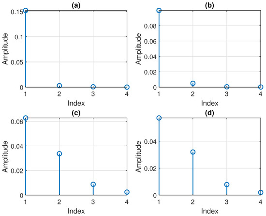
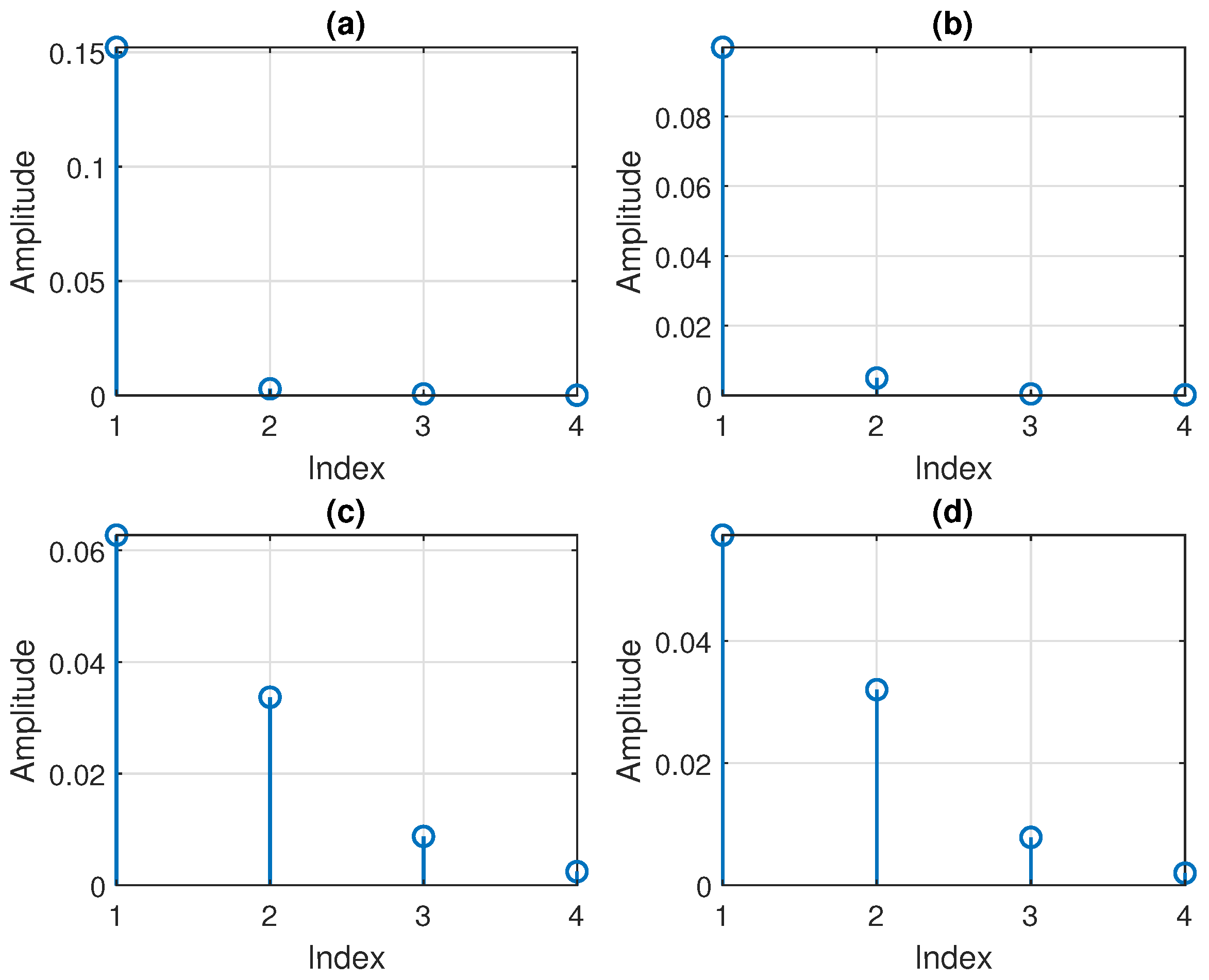
At this point, the lengths of the component impulse responses can also be factorized as $L_1=L_{11}{L}_{12}$ and $L_2=L_{21}{L}_{22}$, with $L_{11}\ge L_{12}$ and $L_{21}\ge L_{22}$. For example, using the AIR from Figure 2a, with $L_1=L_2=32$, the factorization could be performed with $L_{11}=8$, $L_{12}=4$, $L_{21}=8$, and $L_{22}=4$. The component impulse responses from (1), i.e., ${\mathbf{h}}_2^r$ and ${\mathbf{h}}_1^r$ (with $r=1,2,\dots ,R$), also possess the low-rank property. In other words, their corresponding matrices, denoted by ${\mathbf{H}}_2^r$ and ${\mathbf{H}}_1^r$ (of sizes $L_{21}\times L_{22}$ and $L_{11}\times L_{12}$, respectively), are not full-rank. This is supported in Figure 4, where the singular values of the matrix ${\mathbf{H}}_2^r$ (of size $8\times 4$) are depicted for $r=1,2,3$ and 4. Again, these values decrease to zero, so the approximated rank of ${\mathbf{H}}_2^r$ could be around $L_{22}/2$.

Figure 4. Singular values of the matrix ${\mathbf{H}}_2^r$ (of size $8\times 4$) for the corresponding impulse response ${\mathbf{h}}_2^r$ (of length $L_2=32$), with (a) $r=1$, (b) $r=2$, (c) $r=3$, and (d) $r=4$.

As a result, based on the same low-rank considerations, a similar decomposition as in (1) can be applied to ${\mathbf{h}}_1^r$ and ${\mathbf{h}}_2^r$, with $r=1,2,\dots ,R$, such that

$$\begin{array}{cc}\hfill {\mathbf{h}}_1^r& =\sum _{p=1}^P{\mathbf{h}}_{12}^{rp}\otimes {\mathbf{h}}_{11}^{rp},\hfill \end{array}$$

(2)

$$\begin{array}{cc}\hfill {\mathbf{h}}_2^r& =\sum _{q=1}^Q{\mathbf{h}}_{22}^{rq}\otimes {\mathbf{h}}_{21}^{rq},\hfill \end{array}$$

(3)

where $P<L_{12}$ and $Q<L_{22}$ represent the (approximated) ranks of the corresponding matrices associated with ${\mathbf{h}}_1^r$ and ${\mathbf{h}}_2^r$ (i.e., ${\mathbf{H}}_1^r$ and ${\mathbf{H}}_2^r$, respectively); here, the vectors ${\mathbf{h}}_{11}^{rp}$, ${\mathbf{h}}_{12}^{rp}$, ${\mathbf{h}}_{21}^{rq}$, and ${\mathbf{h}}_{22}^{rq}$ correspond to four impulse responses of lengths $L_{11}$, $L_{12}$, $L_{21}$, and $L_{22}$, respectively. Thus, the current factorization of the global length is $L=L_{11}{L}_{12}{L}_{21}{L}_{22}$. As a result, substituting (2) and (3) into (1), then rearranging the terms within the sums, the global impulse response results in

$$\begin{array}{cc}\hfill \mathbf{h}& =\sum _{r=1}^R\sum _{p=1}^P\sum _{q=1}^Q{\mathbf{h}}_{22}^{rq}\otimes {\mathbf{h}}_{21}^{rq}\otimes {\mathbf{h}}_{12}^{rp}\otimes {\mathbf{h}}_{11}^{rp}.\hfill \end{array}$$

(4)

An equivalent representation of (4) in a fourth-order tensor form is

$$\begin{array}{cc}\hfill \mathcal{H}& =\sum _{p=1}^P\sum _{q=1}^Q\left(\sum _{r=1}^R{\mathbf{h}}_{11}^{rp}\circ {\mathbf{h}}_{12}^{rp}\circ {\mathbf{h}}_{21}^{rq}\circ {\mathbf{h}}_{22}^{rq}\right),\hfill \end{array}$$

(5)

where ∘ denotes the outer product, and the term within the brackets represents a fourth-order tensor of rank R. In fact, this corresponds to the canonical polyadic (CP) decomposition [32], where a fourth-order tensor of rank R is factorized into a sum of R fourth-order tensors of rank-1, i.e., ${\mathbf{h}}_{11}^{rp}\circ {\mathbf{h}}_{12}^{rp}\circ {\mathbf{h}}_{21}^{rq}\circ {\mathbf{h}}_{22}^{rq}\in {\mathbb{R}}^{L_{11}\times L_{12}\times L_{21}\times L_{22}}$, with $r=1,2,\dots ,R$. Therefore, the tensor $\mathcal{H}$ from (5) is obtained as a double-sum of $PQ$ fourth-order tensors, each one of rank R. It can be noticed that the rank of $\mathcal{H}$ is known and can be controlled by setting the value of R in the first step of the decomposition from (1). The decomposition related to (4) or (5) is similar to the one introduced in [47]. However, in the current development, the low-rank framework is used from the beginning in (1). On the other hand, the decomposition from [47] considers the full-rank representation of $\mathbf{h}$ using $L_2$ instead of R in the sum from (1), thus leading to a higher complexity order.

3. RLS-FOT Algorithm

Following the AEC scheme from Figure 1, let us consider that $\widehat{\mathbf{h}}\left(n\right)$ is an estimate of $\mathbf{h}$ at time index n, i.e., an adaptive filter of length L, with real-valued coefficients. In order to exploit (4) for this system identification problem, the impulse response of the adaptive filter can be similarly expressed as

$$\begin{array}{cc}\hfill \widehat{\mathbf{h}}\left(n\right)& =\sum _{r=1}^R\sum _{p=1}^P\sum _{q=1}^Q{\widehat{\mathbf{h}}}_{22}^{rq}\left(n\right)\otimes {\widehat{\mathbf{h}}}_{21}^{rq}\left(n\right)\otimes {\widehat{\mathbf{h}}}_{12}^{rp}\left(n\right)\otimes {\widehat{\mathbf{h}}}_{11}^{rp}\left(n\right),\hfill \end{array}$$

(6)

where ${\widehat{\mathbf{h}}}_{22}^{rq}\left(n\right)$, ${\widehat{\mathbf{h}}}_{21}^{rq}\left(n\right)$, ${\widehat{\mathbf{h}}}_{12}^{rp}\left(n\right)$, and ${\widehat{\mathbf{h}}}_{11}^{rp}\left(n\right)$ represent the estimates of ${\mathbf{h}}_{22}^{rq}$, ${\mathbf{h}}_{21}^{rq}$, ${\mathbf{h}}_{12}^{rp}$, and ${\mathbf{h}}_{11}^{rp}$, respectively. In this context, we should note that this decomposition is not unique since

$$\begin{array}{cc}\hfill {\mathbf{h}}_{22}^{rq}\otimes {\mathbf{h}}_{21}^{rq}\otimes {\mathbf{h}}_{12}^{rp}\otimes {\mathbf{h}}_{11}^{rp}& =a{\mathbf{h}}_{22}^{rq}\otimes b{\mathbf{h}}_{21}^{rq}\otimes c{\mathbf{h}}_{12}^{rp}\otimes d{\mathbf{h}}_{11}^{rp},\hfill \end{array}$$

(7)

with $a,b,c,d\in \mathbb{R}$ and $abcd=1$. However, the main goal is to estimate the global impulse response, $\mathbf{h}$, which is identified without any scaling ambiguity.

Next, for an efficient system identification approach under the decomposition framework, the term from the right-hand side of (6) can be expressed in four alternative ways (using the Kronecker product properties); i.e.,

$$\begin{array}{cc}\hfill {\widehat{\mathbf{h}}}_{22}^{rq}\left(n\right)\otimes {\widehat{\mathbf{h}}}_{21}^{rq}\left(n\right)\otimes {\widehat{\mathbf{h}}}_{12}^{rp}\left(n\right)\otimes {\widehat{\mathbf{h}}}_{11}^{rp}\left(n\right)& =\left[{\mathbf{I}}_{L_{22}}\otimes {\widehat{\mathbf{h}}}_{21}^{rq}\left(n\right)\otimes {\widehat{\mathbf{h}}}_{12}^{rp}\left(n\right)\otimes {\widehat{\mathbf{h}}}_{11}^{rp}\left(n\right)\right]{\widehat{\mathbf{h}}}_{22}^{rq}\left(n\right)\hfill \end{array}$$

(8)

$$\begin{array}{cc}\hfill & =\left[{\widehat{\mathbf{h}}}_{22}^{rq}\left(n\right)\otimes {\mathbf{I}}_{L_{21}}\otimes {\widehat{\mathbf{h}}}_{12}^{rp}\left(n\right)\otimes {\widehat{\mathbf{h}}}_{11}^{rp}\left(n\right)\right]{\widehat{\mathbf{h}}}_{21}^{rq}\left(n\right)\hfill \end{array}$$

(9)

$$\begin{array}{cc}\hfill & =\left[{\widehat{\mathbf{h}}}_{22}^{rq}\left(n\right)\otimes {\widehat{\mathbf{h}}}_{21}^{rq}\left(n\right)\otimes {\mathbf{I}}_{L_{12}}\otimes {\widehat{\mathbf{h}}}_{11}^{rp}\left(n\right)\right]{\widehat{\mathbf{h}}}_{12}^{rp}\left(n\right)\hfill \end{array}$$

(10)

$$\begin{array}{cc}\hfill & =\left[{\widehat{\mathbf{h}}}_{22}^{rq}\left(n\right)\otimes {\widehat{\mathbf{h}}}_{21}^{rq}\left(n\right)\otimes {\widehat{\mathbf{h}}}_{12}^{rp}\left(n\right)\otimes {\mathbf{I}}_{L_{11}}\right]{\widehat{\mathbf{h}}}_{11}^{rp}\left(n\right),\hfill \end{array}$$

(11)

where ${\mathbf{I}}_{L_{\star }}$ generally denotes the identity matrix of size $L_{\star }\times L_{\star }$, with $\star \in \left\{22,21,12,11\right\}$. The expressions (8)–(11) suggest a separation of the individual components for the purpose of extracting each block (of short impulse responses) under a multilinear optimization strategy [49]. In the following, this process is illustrated for the first component filter, while the other three (and their specific notations) are provided in Appendix A.

Let us consider the first set of impulse responses, ${\widehat{\mathbf{h}}}_{22}^{rq}\left(n\right)$, with $r=1,2,\dots ,R$ and $q=1,2,\dots ,Q$. Thus, processing (6) based on (8), the global estimate provided by the adaptive filter can be expressed as

$$\begin{array}{cc}\hfill \widehat{\mathbf{h}}\left(n\right)& =\sum _{r=1}^R\sum _{p=1}^P\sum _{q=1}^Q{\mathbf{H}}_{-22}^{rpq}\left(n\right){\widehat{\mathbf{h}}}_{22}^{rq}\left(n\right)\hfill \\ \hfill & =\sum _{q=1}^Q\sum _{p=1}^P{\mathbf{H}}_{-22}^{:pq}\left(n\right){\widehat{\mathbf{h}}}_{22}^{:q}\left(n\right)\hfill \\ \hfill & =\sum _{q=1}^Q{\mathbf{H}}_{-22}^{:+:q}\left(n\right){\widehat{\mathbf{h}}}_{22}^{:q}\left(n\right)\hfill \\ \hfill & ={\underline{\mathbf{H}}}_{-22}\left(n\right){\widehat{\underline{\mathbf{h}}}}_{22}\left(n\right),\hfill \end{array}$$

(12)

where

$$\begin{array}{cc}\hfill {\mathbf{H}}_{-22}^{rpq}\left(n\right)& ={\mathbf{I}}_{L_{22}}\otimes {\widehat{\mathbf{h}}}_{21}^{rq}\left(n\right)\otimes {\widehat{\mathbf{h}}}_{12}^{rp}\left(n\right)\otimes {\widehat{\mathbf{h}}}_{11}^{rp}\left(n\right)\hfill \end{array}$$

(13)

is a matrix of size $L\times L_{22}$. The matrix

$$\begin{array}{cc}\hfill {\mathbf{H}}_{-22}^{:pq}\left(n\right)& =\left[\begin{array}{cccc}{\mathbf{H}}_{-22}^{1pq}\left(n\right)& {\mathbf{H}}_{-22}^{2pq}\left(n\right)& \dots & {\mathbf{H}}_{-22}^{Rpq}\left(n\right)\end{array}\right]\hfill \end{array}$$

(14)

has the size $L\times R{L}_{22}$. The vector

$$\begin{array}{cc}\hfill {\widehat{\mathbf{h}}}_{22}^{:q}\left(n\right)& =\left[\begin{array}{c}{\widehat{\mathbf{h}}}_{22}^{1q}\left(n\right)\hfill \\ {\widehat{\mathbf{h}}}_{22}^{2q}\left(n\right)\hfill \\ ⋮\hfill \\ {\widehat{\mathbf{h}}}_{22}^{Rq}\left(n\right)\hfill \end{array}\right]\hfill \end{array}$$

(15)

has the length $R{L}_{22}$. The matrix

$$\begin{array}{cc}\hfill {\mathbf{H}}_{-22}^{:+:q}\left(n\right)& =\sum _{p=1}^P{\mathbf{H}}_{-22}^{:pq}\left(n\right)\hfill \end{array}$$

(16)

has the size $L\times R{L}_{22}$,

$$\begin{array}{cc}\hfill {\underline{\mathbf{H}}}_{-22}\left(n\right)& =\left[\begin{array}{cccc}{\mathbf{H}}_{-22}^{:+:1}\left(n\right)& {\mathbf{H}}_{-22}^{:+:2}\left(n\right)& \dots & {\mathbf{H}}_{-22}^{:+:Q}\left(n\right)\end{array}\right]\hfill \end{array}$$

(17)

a matrix of size $L\times QR{L}_{22}$. The vector

$$\begin{array}{cc}\hfill {\widehat{\underline{\mathbf{h}}}}_{22}\left(n\right)& =\left[\begin{array}{c}{\mathbf{h}}_{22}^{:1}\left(n\right)\hfill \\ {\mathbf{h}}_{22}^{:2}\left(n\right)\hfill \\ ⋮\hfill \\ {\mathbf{h}}_{22}^{:Q}\left(n\right)\hfill \end{array}\right]\hfill \end{array}$$

(18)

has $QR{L}_{22}$ coefficients. Similarly, using the notation from Appendix A, (12) can be alternatively expressed as

$$\begin{array}{cc}\hfill \widehat{\mathbf{h}}\left(n\right)& ={\underline{\mathbf{H}}}_{-21}\left(n\right){\widehat{\underline{\mathbf{h}}}}_{21}\left(n\right)\hfill \\ \hfill & ={\underline{\mathbf{H}}}_{-12}\left(n\right){\widehat{\underline{\mathbf{h}}}}_{12}\left(n\right)\hfill \\ \hfill & ={\underline{\mathbf{H}}}_{-11}\left(n\right){\widehat{\underline{\mathbf{h}}}}_{11}\left(n\right).\hfill \end{array}$$

(19)

At this point, according to Figure 1, the a priori error signal, $e\left(n\right)$, results as the difference between the reference/desired signal, $d\left(n\right)$, and the estimated output, $\widehat{y}\left(n\right)={\widehat{\mathbf{h}}}^{\top }(n-1)\mathbf{x}\left(n\right)$, where the superscript ^⊤ denotes transposition. Also, at the discrete-time index n, the signal $d\left(n\right)$ is given by the convolution between the samples of the input signal, $x\left(n\right)$, and the coefficients of the unknown system impulse response ($\mathbf{h}$), corrupted by the near-end signal, $v\left(n\right)$, which is uncorrelated to the input (far-end) signal. Consequently, considering that $x\left(n\right)$ and $v\left(n\right)$ are real-valued sequences, the error signal results in

$$\begin{array}{cc}\hfill e\left(n\right)& =d\left(n\right)-{\mathbf{x}}^{\top }\left(n\right)\widehat{\mathbf{h}}(n-1),\hfill \end{array}$$

(20)

where

$$\begin{array}{cc}\hfill d\left(n\right)& ={\mathbf{x}}^{\top }\left(n\right)\mathbf{h}+v\left(n\right)\hfill \end{array}$$

(21)

and

$$\begin{array}{cc}\hfill \mathbf{x}\left(n\right)& =\left[\begin{array}{c}x\left(n\right)\hfill \\ x(n-1)\hfill \\ ⋮\hfill \\ x(n-L+1)\hfill \end{array}\right].\hfill \end{array}$$

(22)

Then, based on (12) and (19), the error signal from (20) can be further rewritten in four alternative manners:

$$\begin{array}{cc}\hfill e\left(n\right)& =d\left(n\right)-{\mathbf{x}}_{22}^{\top }\left(n\right){\widehat{\underline{\mathbf{h}}}}_{22}(n-1)\hfill \end{array}$$

(23)

$$\begin{array}{cc}\hfill & =d\left(n\right)-{\mathbf{x}}_{21}^{\top }\left(n\right){\widehat{\underline{\mathbf{h}}}}_{21}(n-1)\hfill \end{array}$$

(24)

$$\begin{array}{cc}\hfill & =d\left(n\right)-{\mathbf{x}}_{12}^{\top }\left(n\right){\widehat{\underline{\mathbf{h}}}}_{12}(n-1)\hfill \end{array}$$

(25)

$$\begin{array}{cc}\hfill & =d\left(n\right)-{\mathbf{x}}_{11}^{\top }\left(n\right){\widehat{\underline{\mathbf{h}}}}_{11}(n-1),\hfill \end{array}$$

(26)

where

$$\begin{array}{cc}\hfill {\mathbf{x}}_{22}\left(n\right)& ={\underline{\mathbf{H}}}_{-22}^{\top }(n-1)\mathbf{x}\left(n\right),\hfill \end{array}$$

(27)

$$\begin{array}{cc}\hfill {\mathbf{x}}_{21}\left(n\right)& ={\underline{\mathbf{H}}}_{-21}^{\top }(n-1)\mathbf{x}\left(n\right),\hfill \end{array}$$

(28)

$$\begin{array}{cc}\hfill {\mathbf{x}}_{12}\left(n\right)& ={\underline{\mathbf{H}}}_{-12}^{\top }(n-1)\mathbf{x}\left(n\right),\hfill \end{array}$$

(29)

$$\begin{array}{cc}\hfill {\mathbf{x}}_{11}\left(n\right)& ={\underline{\mathbf{H}}}_{-11}^{\top }(n-1)\mathbf{x}\left(n\right)\hfill \end{array}$$

(30)

represent the “inputs” of the four component filters. In the following, the previous expressions can be used to derive a fourth-order decomposition-based RLS algorithm, with improved performance compared to the conventional RLS filter.

First, from (23) and considering that ${\widehat{\underline{\mathbf{h}}}}_{21}\left(n\right)$, ${\widehat{\underline{\mathbf{h}}}}_{12}\left(n\right)$, and ${\widehat{\underline{\mathbf{h}}}}_{11}\left(n\right)$ are fixed, following the least-squares (LS) optimization criterion, the cost function for the first component filter can be expressed as

$$\begin{array}{cc}\hfill \mathcal{J}\left[{\widehat{\underline{\mathbf{h}}}}_{22}\left(n\right)|{\widehat{\underline{\mathbf{h}}}}_{21},{\widehat{\underline{\mathbf{h}}}}_{12},{\widehat{\underline{\mathbf{h}}}}_{11}\right]& =\sum _{k=1}^n{\lambda }_{22}^{n-k}{\left[d\left(k\right)-{\mathbf{x}}_{22}^{\top }\left(k\right){\widehat{\underline{\mathbf{h}}}}_{22}\left(n\right)\right]}^2\hfill \\ \hfill & =\sum _{k=1}^n{\lambda }_{22}^{n-k}{d}^2\left(k\right)-2{\widehat{\underline{\mathbf{h}}}}_{22}^{\top }\left(n\right){\mathbf{r}}_{22}\left(n\right)+{\widehat{\underline{\mathbf{h}}}}_{22}^{\top }\left(n\right){\mathbf{R}}_{22}\left(n\right){\widehat{\underline{\mathbf{h}}}}_{22}\left(n\right),\hfill \end{array}$$

(31)

where $0<{\lambda }_{22}\le 1$ is a forgetting factor and

$$\begin{array}{cc}\hfill {\mathbf{r}}_{22}\left(n\right)& =\sum _{k=1}^n{\lambda }_{22}^{n-k}{\mathbf{x}}_{22}\left(k\right)d\left(k\right)={\lambda }_{22}{\mathbf{r}}_{22}(n-1)+{\mathbf{x}}_{22}\left(n\right)d\left(n\right),\hfill \end{array}$$

(32)

$$\begin{array}{cc}\hfill {\mathbf{R}}_{22}\left(n\right)& =\sum _{k=1}^n{\lambda }_{22}^{n-k}{\mathbf{x}}_{22}\left(k\right){\mathbf{x}}_{22}^{\top }\left(k\right)={\lambda }_{22}{\mathbf{R}}_{22}(n-1)+{\mathbf{x}}_{22}\left(n\right){\mathbf{x}}_{22}^{\top }\left(n\right).\hfill \end{array}$$

(33)

In a similar manner, following (24) and considering that ${\widehat{\underline{\mathbf{h}}}}_{22}\left(n\right)$, ${\widehat{\underline{\mathbf{h}}}}_{12}\left(n\right)$, and ${\widehat{\underline{\mathbf{h}}}}_{11}\left(n\right)$ are fixed, the second LS cost function can be written as

$$\begin{array}{cc}\hfill \mathcal{J}\left[{\widehat{\underline{\mathbf{h}}}}_{21}\left(n\right)|{\widehat{\underline{\mathbf{h}}}}_{22},{\widehat{\underline{\mathbf{h}}}}_{12},{\widehat{\underline{\mathbf{h}}}}_{11}\right]& =\sum _{k=1}^n{\lambda }_{21}^{n-k}{\left[d\left(k\right)-{\mathbf{x}}_{21}^{\top }\left(k\right){\widehat{\underline{\mathbf{h}}}}_{21}\left(n\right)\right]}^2\hfill \\ \hfill & =\sum _{k=1}^n{\lambda }_{21}^{n-k}{d}^2\left(k\right)-2{\widehat{\underline{\mathbf{h}}}}_{21}^{\top }\left(n\right){\mathbf{r}}_{21}\left(n\right)+{\widehat{\underline{\mathbf{h}}}}_{21}^{\top }\left(n\right){\mathbf{R}}_{21}\left(n\right){\widehat{\underline{\mathbf{h}}}}_{21}\left(n\right),\hfill \end{array}$$

(34)

with $0<{\lambda }_{21}\le 1$ and

$$\begin{array}{cc}\hfill {\mathbf{r}}_{21}\left(n\right)& =\sum _{k=1}^n{\lambda }_{21}^{n-k}{\mathbf{x}}_{21}\left(k\right)d\left(k\right)={\lambda }_{21}{\mathbf{r}}_{21}(n-1)+{\mathbf{x}}_{21}\left(n\right)d\left(n\right),\hfill \end{array}$$

(35)

$$\begin{array}{cc}\hfill {\mathbf{R}}_{21}\left(n\right)& =\sum _{k=1}^n{\lambda }_{21}^{n-k}{\mathbf{x}}_{21}\left(k\right){\mathbf{x}}_{21}^{\top }\left(k\right)={\lambda }_{21}{\mathbf{R}}_{21}(n-1)+{\mathbf{x}}_{21}\left(n\right){\mathbf{x}}_{21}^{\top }\left(n\right).\hfill \end{array}$$

(36)

Next, based on (25) and considering that ${\widehat{\underline{\mathbf{h}}}}_{22}\left(n\right)$, ${\widehat{\underline{\mathbf{h}}}}_{21}\left(n\right)$, and ${\widehat{\underline{\mathbf{h}}}}_{11}\left(n\right)$ are fixed, the third LS cost function becomes

$$\begin{array}{cc}\hfill \mathcal{J}\left[{\widehat{\underline{\mathbf{h}}}}_{12}\left(n\right)|{\widehat{\underline{\mathbf{h}}}}_{22},{\widehat{\underline{\mathbf{h}}}}_{21},{\widehat{\underline{\mathbf{h}}}}_{11}\right]& =\sum _{k=1}^n{\lambda }_{12}^{n-k}{\left[d\left(k\right)-{\mathbf{x}}_{12}^{\top }\left(k\right){\widehat{\underline{\mathbf{h}}}}_{12}\left(n\right)\right]}^2\hfill \\ \hfill & =\sum _{k=1}^n{\lambda }_{12}^{n-k}{d}^2\left(k\right)-2{\widehat{\underline{\mathbf{h}}}}_{12}^{\top }\left(n\right){\mathbf{r}}_{12}\left(n\right)+{\widehat{\underline{\mathbf{h}}}}_{12}^{\top }\left(n\right){\mathbf{R}}_{12}\left(n\right){\widehat{\underline{\mathbf{h}}}}_{12}\left(n\right),\hfill \end{array}$$

(37)

where $0<{\lambda }_{12}\le 1$ and

$$\begin{array}{cc}\hfill {\mathbf{r}}_{12}\left(n\right)& =\sum _{k=1}^n{\lambda }_{12}^{n-k}{\mathbf{x}}_{12}\left(k\right)d\left(k\right)={\lambda }_{12}{\mathbf{r}}_{12}(n-1)+{\mathbf{x}}_{12}\left(n\right)d\left(n\right),\hfill \end{array}$$

(38)

$$\begin{array}{cc}\hfill {\mathbf{R}}_{12}\left(n\right)& =\sum _{k=1}^n{\lambda }_{12}^{n-k}{\mathbf{x}}_{12}\left(k\right){\mathbf{x}}_{12}^{\top }\left(k\right)={\lambda }_{12}{\mathbf{R}}_{12}(n-1)+{\mathbf{x}}_{12}\left(n\right){\mathbf{x}}_{12}^{\top }\left(n\right).\hfill \end{array}$$

(39)

Finally, from (26) and considering that ${\widehat{\underline{\mathbf{h}}}}_{22}\left(n\right)$, ${\widehat{\underline{\mathbf{h}}}}_{21}\left(n\right)$, and ${\widehat{\underline{\mathbf{h}}}}_{12}\left(n\right)$ are fixed, the fourth LS cost function is

$$\begin{array}{cc}\hfill \mathcal{J}\left[{\widehat{\underline{\mathbf{h}}}}_{11}\left(n\right)|{\widehat{\underline{\mathbf{h}}}}_{22},{\widehat{\underline{\mathbf{h}}}}_{21},{\widehat{\underline{\mathbf{h}}}}_{12}\right]& =\sum _{k=1}^n{\lambda }_{11}^{n-k}{\left[d\left(k\right)-{\mathbf{x}}_{11}^{\top }\left(k\right){\widehat{\underline{\mathbf{h}}}}_{11}\left(n\right)\right]}^2\hfill \\ \hfill & =\sum _{k=1}^n{\lambda }_{11}^{n-k}{d}^2\left(k\right)-2{\widehat{\underline{\mathbf{h}}}}_{11}^{\top }\left(n\right){\mathbf{r}}_{11}\left(n\right)+{\widehat{\underline{\mathbf{h}}}}_{11}^{\top }\left(n\right){\mathbf{R}}_{11}\left(n\right){\widehat{\underline{\mathbf{h}}}}_{11}\left(n\right),\hfill \end{array}$$

(40)

with $0<{\lambda }_{11}\le 1$ and

$$\begin{array}{cc}\hfill {\mathbf{r}}_{11}\left(n\right)& =\sum _{k=1}^n{\lambda }_{11}^{n-k}{\mathbf{x}}_{11}\left(k\right)d\left(k\right)={\lambda }_{11}{\mathbf{r}}_{11}(n-1)+{\mathbf{x}}_{11}\left(n\right)d\left(n\right),\hfill \end{array}$$

(41)

$$\begin{array}{cc}\hfill {\mathbf{R}}_{11}\left(n\right)& =\sum _{k=1}^n{\lambda }_{11}^{n-k}{\mathbf{x}}_{11}\left(k\right){\mathbf{x}}_{11}^{\top }\left(k\right)={\lambda }_{11}{\mathbf{R}}_{11}(n-1)+{\mathbf{x}}_{11}\left(n\right){\mathbf{x}}_{11}^{\top }\left(n\right).\hfill \end{array}$$

(42)

The minimization of (31), (34), (37), and (40) with respect to ${\widehat{\underline{\mathbf{h}}}}_{22}\left(n\right)$, ${\widehat{\underline{\mathbf{h}}}}_{21}\left(n\right)$, ${\widehat{\underline{\mathbf{h}}}}_{12}\left(n\right)$, and ${\widehat{\underline{\mathbf{h}}}}_{11}\left(n\right)$, respectively, leads to the associated sets of normal equations:

$$\begin{array}{cc}\hfill {\mathbf{R}}_{22}\left(n\right){\widehat{\underline{\mathbf{h}}}}_{22}\left(n\right)& ={\mathbf{r}}_{22}\left(n\right),\hfill \end{array}$$

(43)

$$\begin{array}{cc}\hfill {\mathbf{R}}_{21}\left(n\right){\widehat{\underline{\mathbf{h}}}}_{21}\left(n\right)& ={\mathbf{r}}_{21}\left(n\right),\hfill \end{array}$$

(44)

$$\begin{array}{cc}\hfill {\mathbf{R}}_{12}\left(n\right){\widehat{\underline{\mathbf{h}}}}_{12}\left(n\right)& ={\mathbf{r}}_{12}\left(n\right),\hfill \end{array}$$

(45)

$$\begin{array}{cc}\hfill {\mathbf{R}}_{11}\left(n\right){\widehat{\underline{\mathbf{h}}}}_{11}\left(n\right)& ={\mathbf{r}}_{11}\left(n\right).\hfill \end{array}$$

(46)

These can be recursively solved following the line of the RLS algorithm [1,2,3]. In this context, the matrix inversion lemma [2] is used in (33), (36), (39), and (42) to recursively update the inverse of ${\mathbf{R}}_{\star }\left(n\right)$, with $\star \in \left\{22,21,12,11\right\}$. As a result, denoting by ${\mathbf{P}}_{\star }\left(n\right)$ the (recursive) inverse of the associated matrix ${\mathbf{R}}_{\star }\left(n\right)$, this can be evaluated as

$$\begin{array}{cc}\hfill {\mathbf{P}}_{\star }\left(n\right)& ={\displaystyle \frac{1}{{\lambda }_{\star }}}\left[{\mathbf{P}}_{\star }(n-1)-{\mathbf{k}}_{\star }\left(n\right){\mathbf{x}}_{\star }^{\top }\left(n\right){\mathbf{P}}_{\star }(n-1)\right],\hfill \end{array}$$

(47)

where ${\mathbf{k}}_{\star }\left(n\right)$ is the so-called Kalman gain vector [1,2,3], which is defined as

$$\begin{array}{cc}\hfill {\mathbf{k}}_{\star }\left(n\right)& ={\displaystyle \frac{{\mathbf{P}}_{\star }(n-1){\mathbf{x}}_{\star }\left(n\right)}{{\lambda }_{\star }+{\mathbf{x}}_{\star }^{\top }\left(n\right){\mathbf{P}}_{\star }(n-1){\mathbf{x}}_{\star }\left(n\right)}}.\hfill \end{array}$$

(48)

Based on (47) and (48), the update of each component filter can be obtained by developing the solution of the corresponding normal equations from (43)–(46). To this purpose, the recursive relations for the associated cross-correlation vectors ${\mathbf{r}}_{\star }\left(n\right)$ are used, i.e., (32), (35), (38), and (41), together with the solutions of the normal equations from the previous time-index, i.e., ${\widehat{\underline{\mathbf{h}}}}_{\star }(n-1)={\mathbf{P}}_{\star }(n-1){\mathbf{r}}_{\star }(n-1)$. As a result, we can develop

$$\begin{array}{cc}\hfill {\widehat{\underline{\mathbf{h}}}}_{\star }\left(n\right)& ={\mathbf{P}}_{\star }\left(n\right){\mathbf{r}}_{\star }\left(n\right)\hfill \\ \hfill & ={\displaystyle \frac{1}{{\lambda }_{\star }}}\left[{\mathbf{P}}_{\star }(n-1)-{\mathbf{k}}_{\star }\left(n\right){\mathbf{x}}_{\star }^{\top }\left(n\right){\mathbf{P}}_{\star }(n-1)\right]\left[{\lambda }_{\star }{\mathbf{r}}_{\star }(n-1)+{\mathbf{x}}_{\star }\left(n\right)d\left(n\right)\right]\hfill \\ \hfill & ={\widehat{\underline{\mathbf{h}}}}_{\star }(n-1)+{\mathbf{k}}_{\star }\left(n\right)\left[d\left(n\right)-{\mathbf{x}}_{\star }^{\top }\left(n\right){\widehat{\underline{\mathbf{h}}}}_{\star }(n-1)\right]\hfill \\ \hfill & ={\widehat{\underline{\mathbf{h}}}}_{\star }(n-1)+{\mathbf{k}}_{\star }\left(n\right)e\left(n\right),\hfill \end{array}$$

(49)

where the error signal is defined in (23)–(26). Finally, the components of ${\widehat{\underline{\mathbf{h}}}}_{\star }\left(n\right)$ can be extracted regarding the global estimate $\widehat{\underline{\mathbf{h}}}\left(n\right)$ results based on (6). The resulting RLS algorithm based on FOT decomposition, namely RLS-FOT, is summarized in Algorithm 1.

Algorithm 1: RLS-FOT Algorithm

1: Data: input signal $x\left(n\right)$, reference/desired signal $d\left(n\right)$ 2: Decomposition: $L=L_{11}{L}_{12}{L}_{21}{L}_{22},R<L_{21}{L}_{22},P<L_{12},Q<L_{22}$ 3: Forgetting factors: $0<{\lambda }_{\star }\le 1$, with $\star \in \left\{22,21,12,11\right\}$ Initialization: 4: ${\mathbf{P}}_{22}\left(0\right)={ϵ}^{-1}{\mathbf{I}}_{RQ{L}_{22}},{\mathbf{P}}_{21}\left(0\right)={ϵ}^{-1}{\mathbf{I}}_{RQ{L}_{21}},{\mathbf{P}}_{12}\left(0\right)={ϵ}^{-1}{\mathbf{I}}_{RP{L}_{12}},{\mathbf{P}}_{11}\left(0\right)={ϵ}^{-1}{\mathbf{I}}_{RP{L}_{11}},ϵ>0$ 5: ${\widehat{\mathbf{h}}}_{22}^{rq}\left(0\right)=\left[\begin{array}{c}\epsilon \\ {\mathbf{0}}_{L_{22}-1}\end{array}\right],{\widehat{\mathbf{h}}}_{21}^{rq}\left(0\right)=\left[\begin{array}{c}\epsilon \\ {\mathbf{0}}_{L_{21}-1}\end{array}\right],{\widehat{\mathbf{h}}}_{12}^{rp}\left(0\right)=\left[\begin{array}{c}\epsilon \\ {\mathbf{0}}_{L_{12}-1}\end{array}\right],{\widehat{\mathbf{h}}}_{11}^{rp}\left(0\right)=\left[\begin{array}{c}\epsilon \\ {\mathbf{0}}_{L_{11}-1}\end{array}\right],$ with $r=1,2,\dots ,R,p=1,2,\dots ,P,q=1,2,\dots ,Q,\epsilon >0$ 6: Construct: ${\widehat{\underline{\mathbf{h}}}}_{\star }\left(0\right)$ and ${\underline{\mathbf{H}}}_{-\star }\left(0\right)$, with $\star \in \left\{22,21,12,11\right\}$, as shown in (12)–(18) and Appendix A $\underline{\mathrm{Iterations}}:$ 7: for $n=1,2,\dots$ and $\star \in \left\{22,21,12,11\right\}$ 8: $\mathbf{x}\left(n\right)={\left[\begin{array}{cccc}x\left(n\right)& x(n-1)& \dots & x(n-L+1)\end{array}\right]}^{\top }$ 9: ${\mathbf{x}}_{\star }\left(n\right)={\underline{\mathbf{H}}}_{-\star }^{\top }(n-1)\mathbf{x}\left(n\right)$ 10: $e\left(n\right)=d\left(n\right)-{\mathbf{x}}_{\star }^{\top }\left(n\right){\widehat{\underline{\mathbf{h}}}}_{\star }(n-1)$ 11: ${\mathbf{k}}_{\star }\left(n\right)={\displaystyle \frac{{\mathbf{P}}_{\star }(n-1){\mathbf{x}}_{\star }\left(n\right)}{{\lambda }_{\star }+{\mathbf{x}}_{\star }^{\top }\left(n\right){\mathbf{P}}_{\star }(n-1){\mathbf{x}}_{\star }\left(n\right)}}$ 12: ${\mathbf{P}}_{\star }\left(n\right)={\displaystyle \frac{1}{{\lambda }_{\star }}}\left[{\mathbf{P}}_{\star }(n-1)-{\mathbf{k}}_{\star }\left(n\right){\mathbf{x}}_{\star }^{\top }\left(n\right){\mathbf{P}}_{\star }(n-1)\right]$ 13: ${\widehat{\underline{\mathbf{h}}}}_{\star }\left(n\right)={\widehat{\underline{\mathbf{h}}}}_{\star }(n-1)+{\mathbf{k}}_{\star }\left(n\right)e\left(n\right)$ 14: Construct ${\underline{\mathbf{H}}}_{-\star }\left(n\right)$ and extract ${\widehat{\mathbf{h}}}_{22}^{rq}\left(n\right),{\widehat{\mathbf{h}}}_{21}^{rq}\left(n\right),{\widehat{\mathbf{h}}}_{12}^{rp}\left(n\right),{\widehat{\mathbf{h}}}_{11}^{rp}\left(n\right),$ $\mathrm{with}r=1,2,\dots ,R,p=1,2,\dots ,P,q=1,2,\dots ,Q$ 15: $\widehat{\mathbf{h}}\left(n\right)={\displaystyle \sum _{r=1}^R\sum _{p=1}^P\sum _{q=1}^Q}{\widehat{\mathbf{h}}}_{22}^{rq}\left(n\right)\otimes {\widehat{\mathbf{h}}}_{21}^{rq}\left(n\right)\otimes {\widehat{\mathbf{h}}}_{12}^{rp}\left(n\right)\otimes {\widehat{\mathbf{h}}}_{11}^{rp}\left(n\right)$

It can be noticed that the update of each component filter can be alternatively expressed as

$$\begin{array}{cc}\hfill {\widehat{\underline{\mathbf{h}}}}_{\star }\left(n\right)& ={\widehat{\underline{\mathbf{h}}}}_{\star }(n-1)+{\mathbf{P}}_{\star }\left(n\right){\mathbf{x}}_{\star }\left(n\right)e\left(n\right),\hfill \end{array}$$

(50)

with $\star \in \left\{22,21,12,11\right\}$ since ${\mathbf{k}}_{\star }\left(n\right)={\mathbf{P}}_{\star }\left(n\right){\mathbf{x}}_{\star }\left(n\right)$. This can be further formulated in terms of the misalignment vector, which is defined as ${\mathbf{m}}_{\star }\left(n\right)={\underline{\mathbf{h}}}_{\star }-{\widehat{\underline{\mathbf{h}}}}_{\star }\left(n\right)$, where ${\underline{\mathbf{h}}}_{\star }$ represents the “true” component impulse response. Thus, (50) becomes

$$\begin{array}{cc}\hfill {\mathbf{m}}_{\star }\left(n\right)& ={\mathbf{m}}_{\star }(n-1)-{\mathbf{P}}_{\star }\left(n\right){\mathbf{x}}_{\star }\left(n\right)e\left(n\right).\hfill \end{array}$$

(51)

According to (23)–(26), $e\left(n\right)=d\left(n\right)-{\mathbf{x}}_{\star }^{\top }\left(n\right){\widehat{\underline{\mathbf{h}}}}_{\star }(n-1)$. Also, the reference signal from (21) can be alternatively written as $d\left(n\right)={\mathbf{x}}_{\star }^{\top }\left(n\right){\underline{\mathbf{h}}}_{\star }+v\left(n\right)$, assuming time-invariant systems to be identified. Consequently, the update from (51) results in

$$\begin{array}{cc}\hfill {\mathbf{m}}_{\star }\left(n\right)& ={\mathbf{m}}_{\star }(n-1)-{\mathbf{P}}_{\star }\left(n\right){\mathbf{x}}_{\star }\left(n\right){\mathbf{x}}_{\star }^{\top }\left(n\right){\mathbf{m}}_{\star }(n-1)-{\mathbf{P}}_{\star }\left(n\right){\mathbf{x}}_{\star }\left(n\right)v\left(n\right).\hfill \end{array}$$

(52)

The next goal is to take the mathematical expectation, denoted by $E\left[·\right]$, on both sides of (52), then find a recursive relation for $E\left[{\mathbf{m}}_{\star }\left(n\right)\right]$, which should decay to zero in order to validate the convergence in the mean value of the algorithm. To this purpose, let us consider several supporting assumptions, which facilitate the processing. First, using the recursive relations from (33), (36), (39), and (42), for large enough n, one can approximate

$$\begin{array}{cc}\hfill {\mathbf{R}}_{\star }\left(n\right)& \approx {\displaystyle \frac{E\left[{\mathbf{x}}_{\star }\left(n\right){\mathbf{x}}_{\star }^{\top }\left(n\right)\right]}{1-{\lambda }_{\star }}}.\hfill \end{array}$$

(53)

Also, let us assume that the covariance matrix associated with the input ${\mathbf{x}}_{\star }\left(n\right)$, i.e., $E\left[{\mathbf{x}}_{\star }\left(n\right){\mathbf{x}}_{\star }^{\top }\left(n\right)\right]$, is dominated by its main diagonal, which contains the elements ${\sigma }_{{\mathbf{x}}_{\star }}^2$, i.e., the variance of ${\mathbf{x}}_{\star }\left(n\right)$. This supposition holds especially for white Gaussian inputs and considering nearly statistically independent components in (1). While the assumption on the character of the input signal could look restrictive, it is only used to simplify the processing of (52) in terms of expectation. Therefore, under these circumstances and knowing that ${\mathbf{P}}_{\star }\left(n\right)={\mathbf{R}}_{\star }^{-1}\left(n\right)$, we obtain

$$\begin{array}{cc}\hfill E\left[{\mathbf{m}}_{\star }\left(n\right)\right]& ={\lambda }_{\star }E\left[{\mathbf{m}}_{\star }(n-1)\right]={\lambda }_{\star }^{n}E\left[{\mathbf{m}}_{\star }\left(0\right)\right],\hfill \end{array}$$

(54)

where it is also considered that the input signal and the additive noise are uncorrelated, thus cancelling the last expectation term that results from (52). Since $0<{\lambda }_{\star }\le 1$, the term from the left-hand side of (54) is not increasing with n. In other words, it decays to zero for $n\to \infty$ and subunitary ${\lambda }_{\star }$ so that the algorithm is convergent to the mean value. Note that a rigorous convergence analysis (without supporting assumptions) represents a challenging task due to the connection between the component filters and the specific structures of the “input” signals, ${\mathbf{x}}_{\star }\left(n\right)$, which also incorporate the filter coefficients.

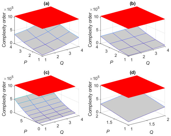
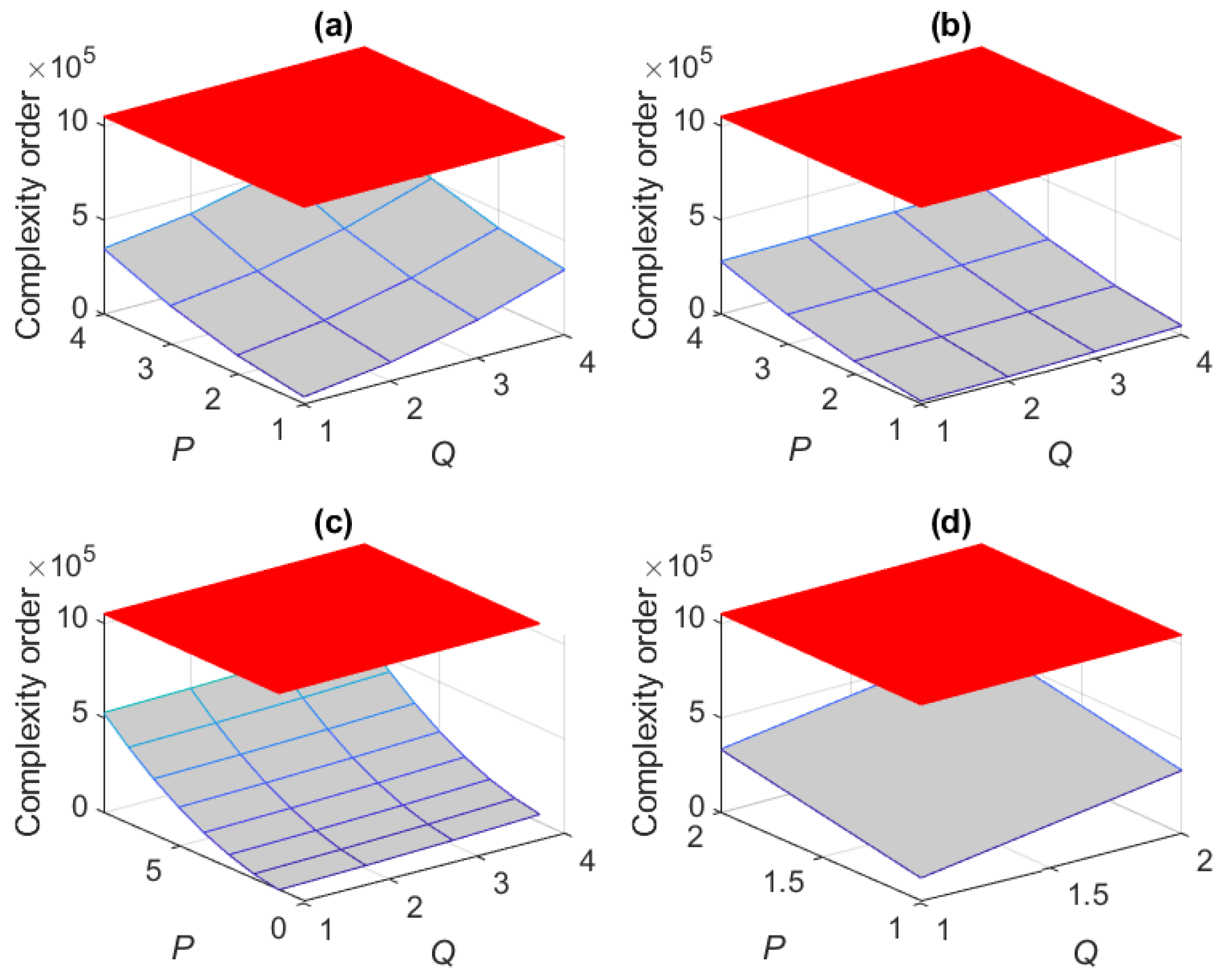
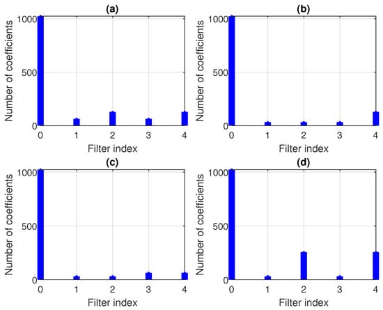
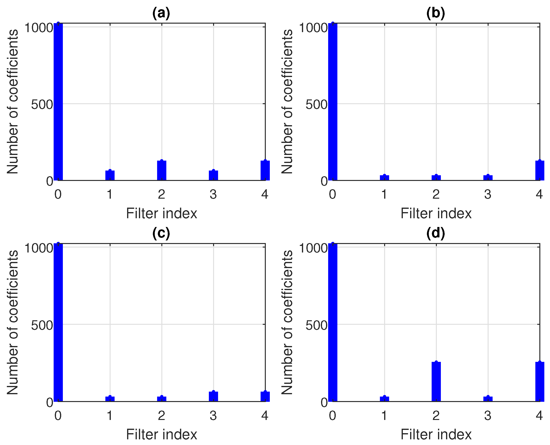
The proposed RLS-FOT combines (in parallel) four RLS-type adaptive filters, which are defined by the impulse responses ${\widehat{\underline{\mathbf{h}}}}_{22}\left(n\right)$, ${\widehat{\underline{\mathbf{h}}}}_{21}\left(n\right)$, ${\widehat{\underline{\mathbf{h}}}}_{12}\left(n\right)$, and ${\widehat{\underline{\mathbf{h}}}}_{11}\left(n\right)$ of lengths $RQ{L}_{22}$, $RQ{L}_{21}$, $RP{L}_{12}$, and $RP{L}_{11}$, respectively, with $R<L_{21}{L}_{22}$, $P<L_{12}$, and $Q<L_{22}$, where $L=L_{11}{L}_{12}{L}_{21}{L}_{22}$. The computational complexity of the conventional RLS algorithm is proportional to the square of the filter length, i.e., $\mathcal{O}\left(L^2\right)$. Therefore, the RLS-FOT has a complexity order of $\mathcal{O}\left[{\left(RQ{L}_{22}\right)}^2+{\left(RQ{L}_{21}\right)}^2+{\left(RP{L}_{12}\right)}^2+{\left(RP{L}_{11}\right)}^2\right]$. For example, let us consider the length of the impulse responses from Figure 2, i.e., $L=1024$. Theoretically, this can be factorized in different ways, e.g., (i) $L_{11}=8$, $L_{12}=4$, $L_{21}=8$, $L_{22}=4$, (ii) $L_{11}=16$, $L_{12}=4$, $L_{21}=4$, $L_{22}=4$, (iii) $L_{11}=8$, $L_{12}=8$, $L_{21}=4$, $L_{22}=4$, and (iv) $L_{11}=16$, $L_{12}=2$, $L_{21}=16$, $L_{22}=2$. Following the discussion related to Figure 3, the value of R could be set as $L_{21}{L}_{22}/2$. In this case, the computational complexity order of the RLS-FOT is depicted in Figure 5, with respect to P and Q, considering the previous four decomposition scenarios, i.e., (i)–(iv). The red surface indicates the complexity order of the conventional RLS algorithm. It can be noticed that the RLS-FOT could be much more advantageous in terms of computational complexity. Furthermore, Figure 6 plots the parameter space of the conventional RLS and RLS-FOT using the same decomposition setups (i)–(iv) with $R=L_{21}{L}_{22}/2$ and $P=Q=1$ in terms of the number of coefficients (of the component filters). The filter index “0” corresponds to the conventional RLS algorithm, which updates a single (long-length) adaptive filter, while the filters “1”–“4” are associated with the four components of the RLS-FOT, i.e., ${\widehat{\underline{\mathbf{h}}}}_{\star }\left(n\right)$, with $\star \in \left\{22,21,12,11\right\}$. Clearly, the parameter space of the RLS-FOT could be significantly smaller compared to the RLS counterpart, and some decomposition setups seem more advantageous than others.

Figure 5. Computational complexity order of the conventional RLS algorithm with $L=1024$ (red surface) and the RLS-FOT using $R=L_{21}{L}_{22}/2$, (a) $L_{11}=8$, $L_{12}=4$, $L_{21}=8$, $L_{22}=4$, (b) $L_{11}=16$, $L_{12}=4$, $L_{21}=4$, $L_{22}=4$, (c) $L_{11}=8$, $L_{12}=8$, $L_{21}=4$, $L_{22}=4$, and (d) $L_{11}=16$, $L_{12}=2$, $L_{21}=16$, $L_{22}=2$.

Figure 6. Parameter space of the conventional RLS algorithm (filter index “0” of length $L=1024$) and the RLS-FOT (filter index “1”–“4”) using $R=L_{21}{L}_{22}/2$, $P=Q=1$, (a) $L_{11}=8$, $L_{12}=4$, $L_{21}=8$, $L_{22}=4$, (b) $L_{11}=16$, $L_{12}=4$, $L_{21}=4$, $L_{22}=4$, (c) $L_{11}=8$, $L_{12}=8$, $L_{21}=4$, $L_{22}=4$, and (d) $L_{11}=16$, $L_{12}=2$, $L_{21}=16$, $L_{22}=2$.

Considering the same example with $L=L_{11}{L}_{12}{L}_{21}{L}_{22}=1024$ and $R=L_{21}{L}_{22}/2$ using the first scenario with $L_{11}=8$, $L_{12}=4$, $L_{21}=8$, $L_{22}=4$, and $P=Q=1$, it results in a parallel combination of four adaptive filters of lengths 64, 128, 64, and 128. In other words, the parameter space is reduced from 1024 coefficients (of the conventional RLS) to a total of 384 coefficients required by the RLS-FOT. Nevertheless, since $L_2=L_{21}{L}_{22}$ is the term that influences the computational complexity of all the component filters, via the parameter R, we can target a lower value for this factor. For example, using the second decomposition scenario with $L_{11}=16$, $L_{12}=4$, $L_{21}=4$, and $L_{22}=4$, under the same circumstances (i.e., $R=L_{21}{L}_{22}/2$ and $P=Q=1$), the parameter space of the RLS-FOT contains $32+32+32+128=244$ coefficients. Following the same reasoning, the third scenario seems even more appealing, i.e., $L_{11}=8$, $L_{12}=8$, $L_{21}=4$, and $L_{22}=4$, with $R=L_{21}{L}_{22}/2$ and $P=Q=1$. In this case, the RLS-FOT updates only $32+32+64+64=192$ coefficients. The fourth decomposition scenario (i.e., $L_{11}=16$, $L_{12}=2$, $L_{21}=16$, and $L_{22}=2$) leads to a larger parameter space (with 576 coefficients) compared to scenarios (i)–(iii). However, it is still significantly below the conventional RLS algorithm. In this context, we should note that using $P=Q=1$ is not a trivial choice taking into account the rank representation from Figure 4. By increasing the values of these decomposition parameters, we obtain a better approximation of the corresponding ranks while paying with increased computational complexity. Nevertheless, since the RLS-FOT combines shorter adaptive filters, its convergence/tracking behavior should be better compared to the conventional RLS algorithm, as will be supported in Section 4.

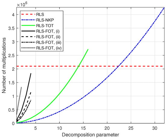
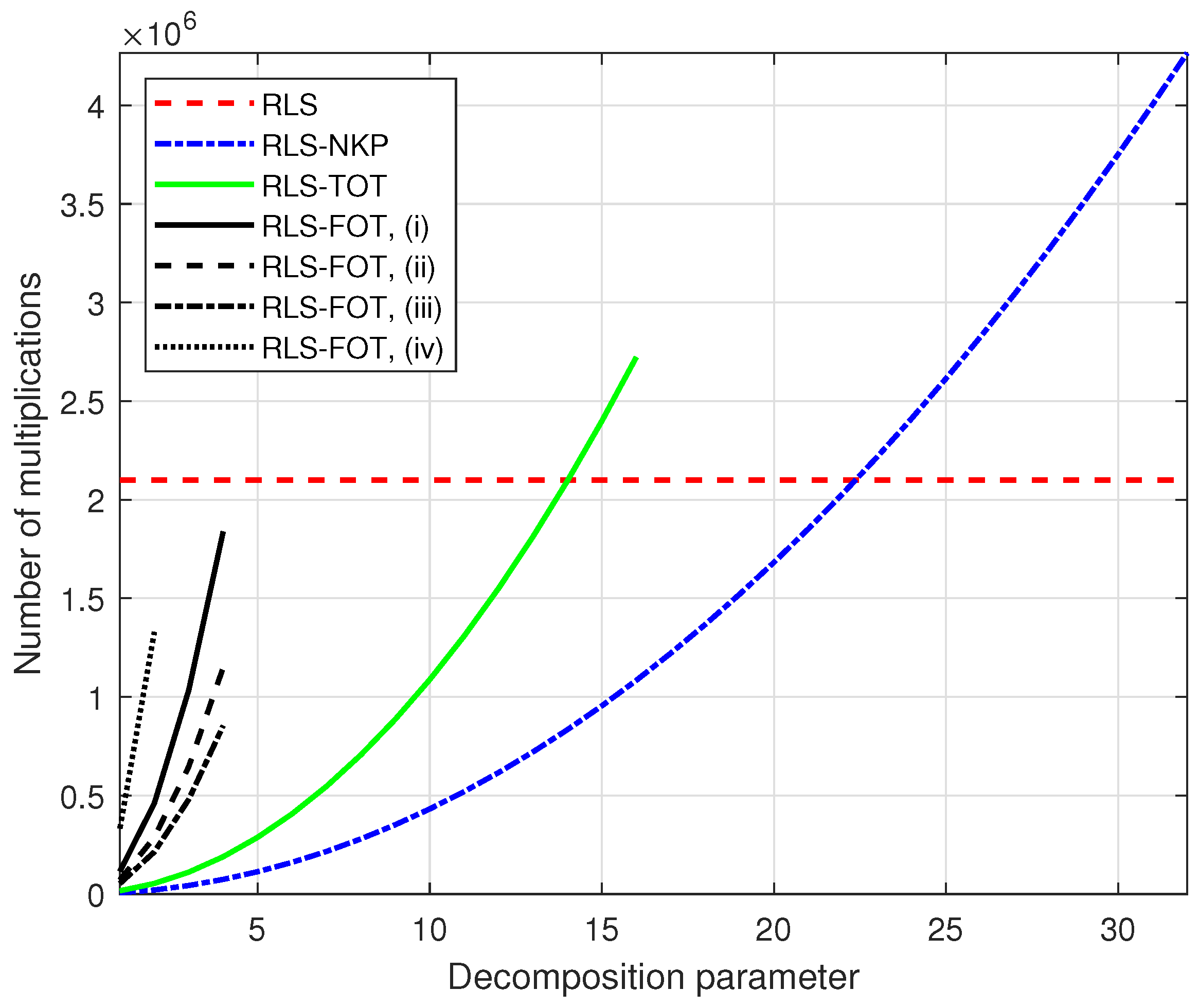
It is interesting to compare the computational complexity of the proposed RLS-FOT with its previously developed counterparts based on the second-order and third-order decompositions. They are referred to as the RLS algorithm based on the nearest Kronecker product (RLS-NKP) [27] and the RLS algorithm based on a third-order tensor decomposition (RLS-TOT) [29], respectively. The RLS-NKP is based on (1) using the factorization $L=L_1{L}_2$ (with $L_1\ge L_2$) and combines two adaptive filters of lengths $R{L}_2$ and $R{L}_1$, with $R\le L_2$ (hence, R plays a similar role as in the RLS-FOT, thus keeping the same notation). As a result, its computational complexity order is $\mathcal{O}\left[{\left(R{L}_2\right)}^2+{\left(R{L}_1\right)}^2\right]$. The RLS-TOT expresses the length of the global filter as $L=L_1^{\prime }{L}_2^{\prime }$, with $L_1^{\prime }\gg L_2^{\prime }$, while the first dimension is also factorized as $L_1^{\prime }=L_{11}^{\prime }{L}_{12}^{\prime }$ (with $L_{11}^{\prime }\ge L_{12}^{\prime }$). It combines three adaptive filters of lengths ${L_2^{\prime }}^2$, $M{L}_{12}^{\prime }{L}_2^{\prime }$, and $M{L}_{11}^{\prime }{L}_2^{\prime }$, with $M\le L_{12}^{\prime }$, thus having the computational complexity order $\mathcal{O}\left[{\left(L_2^{\prime }\right)}^4+{\left(M{L}_{12}^{\prime }{L}_2^{\prime }\right)}^2+{\left(M{L}_{11}^{\prime }{L}_2^{\prime }\right)}^2\right]$. In order to compare the computational complexities of these decomposition-based algorithms on the same (2D) representation, using their corresponding decomposition parameters on the x-axis, we set $P=Q$ for the RLS-FOT, with $Q\le L_{22}$; the decomposition parameters for the RLS-NKP [27] and RLS-TOT [29] are R and M, respectively (as explained before). Following the previous example with $L=1024$, the factorization for the RLS-NKP is $L_1=L_2=32$, while the RLS-TOT uses $L_{11}^{\prime }=32$, $L_{12}^{\prime }=16$, and $L_2^{\prime }=2$. For the RLS-FOT, we consider the same four scenarios (i)–(iv) that have been previously analyzed, with $R=L_{21}{L}_{22}/2$. The results of such a comparison are depicted in Figure 7 in terms of the number of multiplications (per iteration), as detailed in Table 1. As we can notice, for large values of R and M, the computational amounts of RLS-NKP and RLS-TOT could exceed the computational complexity of the conventional RLS algorithm, which is expected. However, they do not operate in that zone since their decomposition parameters are usually selected as $R<L_2/2$ [27] and $M<L_{12}/2$ [29]. On the other hand, the computational complexity of the RLS-FOT is always below the conventional RLS benchmark for all the values of P and Q.

Figure 7. Computational complexity in terms of the number of multiplications (per iteration) of the conventional RLS algorithm ($L=1024$), RLS-NKP [27] (with $L_1=L_2=32$ and $R\le L_2$), RLS-TOT [29] (with $L_{11}^{\prime }=32$, $L_{12}^{\prime }=16$, $L_2^{\prime }=2$, and $M\le L_{12}^{\prime }$), and RLS-FOT using $R=L_{21}{L}_{22}/2$, $P=Q$, with $Q\le L_{22}$, in different decomposition scenarios, i.e., (i) $L_{11}=8$, $L_{12}=4$, $L_{21}=8$, $L_{22}=4$, (ii) $L_{11}=16$, $L_{12}=4$, $L_{21}=4$, $L_{22}=4$, (iii) $L_{11}=8$, $L_{12}=8$, $L_{21}=4$, $L_{22}=4$, and (iv) $L_{11}=16$, $L_{12}=2$, $L_{21}=16$, $L_{22}=2$.

Table 1. Computational complexity in terms of the number of multiplications (per iteration) of the conventional RLS algorithm, RLS-NKP [27], RLS-TOT [29], and RLS-FOT.

Algorithms	Number of Multiplications
RLS	$2L^2+2L$
RLS-NKP [27]	$2{\left(R{L}_2\right)}^2+2{\left(R{L}_1\right)}^2+3R{L}_2+2R{L}_1+2RL$
RLS-TOT [29]	$2{\left(L_2^{\prime }\right)}^4+2{\left(M{L}_{12}^{\prime }{L}_2^{\prime }\right)}^2+2{\left(M{L}_{11}^{\prime }{L}_2^{\prime }\right)}^2+3{\left(L_2^{\prime }\right)}^2+2\left(M{L}_{12}^{\prime }{L}_2^{\prime }\right)+2\left(M{L}_{11}^{\prime }{L}_2^{\prime }\right)+3M{L}_2^{\prime }L$
RLS-FOT	$2{\left(RQ{L}_{22}\right)}^2+2{\left(RQ{L}_{21}\right)}^2+2{\left(RP{L}_{12}\right)}^2+2{\left(RP{L}_{11}\right)}^2+2\left(RQ{L}_{22}\right)+2\left(RQ{L}_{21}\right)+2\left(RP{L}_{12}\right)+2\left(RP{L}_{11}\right)+\max \left[RQ{L}_{22},RQ{L}_{21},RP{L}_{12},RP{L}_{11}\right]+4RQPL$

The computational complexity of the RLS-FOT reported in Table 1 has been evaluated based on the main lines of the algorithm summarized in Algorithm 1. The most “expensive” operations are those involving matrix multiplications. For example, the terms ${\mathbf{P}}_{\star }(n-1){\mathbf{x}}_{\star }\left(n\right)$, with $\star \in \left\{22,21,12,11\right\}$, require ${\left(RQ{L}_{22}\right)}^2+{\left(RQ{L}_{21}\right)}^2+{\left(RP{L}_{12}\right)}^2+{\left(RP{L}_{11}\right)}^2$ multiplications. These terms appear within the Kalman gain vectors, ${\mathbf{k}}_{\star }\left(n\right)$, and also in the update of the matrices ${\mathbf{P}}_{\star }\left(n\right)$, in the transpose forms ${\mathbf{x}}_{\star }^{\top }\left(n\right){\mathbf{P}}_{\star }(n-1)$. The multiplications of the Kalman gain vectors ${\mathbf{k}}_{\star }\left(n\right)$ with these transpose terms are further required within the updates of the matrices ${\mathbf{P}}_{\star }\left(n\right)$, thus needing an extra ${\left(RQ{L}_{22}\right)}^2+{\left(RQ{L}_{21}\right)}^2+{\left(RP{L}_{12}\right)}^2+{\left(RP{L}_{11}\right)}^2$ multiplications. These computational amounts proportional to the squares of the filters’ lengths represent the dominant factors in terms of computational complexity, as indicated in the last line of Table 1, related to the first four terms. They also give the complexity order of the RLS-FOT, which is proportional to the sum of the squares of the filters’ lengths, as indicated before (related to Figure 5). Moreover, there are other operations that require a computational amount proportional to the filters’ lengths. For example, the multiplication between the Kalman gain vectors and the error signal, i.e., ${\mathbf{k}}_{\star }\left(n\right)e\left(n\right)$, which are required within the filters’ updates, need $RQ{L}_{22}+RQ{L}_{21}+RP{L}_{12}+RP{L}_{11}$ multiplications. The same computational amount is needed for the multiplications between ${\mathbf{x}}_{\star }^{\top }\left(n\right)$ and the vectors ${\mathbf{P}}_{\star }(n-1){\mathbf{x}}_{\star }\left(n\right)$ (that are already available), which appear at the denominator of the Kalman gain vectors. Since $e\left(n\right)$ can be expressed in four alternative forms, as indicated in (23)–(26), the product ${\mathbf{x}}_{\star }^{\top }\left(n\right){\widehat{\underline{\mathbf{h}}}}_{\star }(n-1)$ can be evaluated for the shortest component filter, thus requiring $\max \left[RQ{L}_{22},RQ{L}_{21},RP{L}_{12},RP{L}_{11}\right]$ multiplications. Finally, the evaluation of the “input” signals ${\mathbf{x}}_{\star }\left(n\right)$, with $\star \in \left\{22,21,12,11\right\}$, involves a total of $4RQPL$ multiplications due to the specific structures of the matrices ${\underline{\mathbf{H}}}_{-\star }(n-1)$.

The main convergence parameters of the RLS-FOT are the four forgetting factors, ${\lambda }_{\star }$, with $\star \in \left\{22,21,12,11\right\}$. These are positive subunitary constants, which are related to the “memory” of the algorithm, as indicated by the cost functions (31), (34), (37), and (40). In other words, they are used to gradually “forget” the past errors in order to properly operate in time-varying environments. The conventional RLS algorithm uses a similar forgetting factor [1,2,3], denoted by $\lambda$, which is usually set as

$$\begin{array}{cc}\hfill \lambda & =1-{\displaystyle \frac{1}{\kappa L}},\hfill \end{array}$$

(55)

with $\kappa \ge 1$ being a positive integer. Naturally, the forgetting factor is set depending on the filter length since it is a memory-related parameter. Consequently, in the case of RLS-FOT, its four forgetting factors can be set following the same rule, i.e.,

$$\begin{array}{cc}\hfill {\lambda }_{22}& =1-{\displaystyle \frac{1}{\kappa RQ{L}_{22}}},\hfill \end{array}$$

(56)

$$\begin{array}{cc}\hfill {\lambda }_{21}& =1-{\displaystyle \frac{1}{\kappa RQ{L}_{21}}},\hfill \end{array}$$

(57)

$$\begin{array}{cc}\hfill {\lambda }_{12}& =1-{\displaystyle \frac{1}{\kappa RP{L}_{12}}},\hfill \end{array}$$

(58)

$$\begin{array}{cc}\hfill {\lambda }_{11}& =1-{\displaystyle \frac{1}{\kappa RP{L}_{11}}}.\hfill \end{array}$$

(59)

Similar approaches have also been used for setting the forgetting factors of other decomposition-based algorithms, e.g., RLS-NKP [27] and RLS-TOT [29], which use two and three such parameters, respectively.

Using these forms of the forgetting factors, the stability of the algorithm can be evaluated based on the so-called conversion factors [1,2,3], which are defined as the ratios between the a posteriori and a priori error signals. The former are defined as ${\tilde{e}}_{\star }\left(n\right)=d\left(n\right)-{\mathbf{x}}_{\star }^{\top }\left(n\right){\widehat{\underline{\mathbf{h}}}}_{\star }\left(n\right)$, with $\star \in \left\{22,21,12,11\right\}$, while the equivalent forms of the a priori error are given in (23)–(26). Based on the updates (50), the relation between these two types of errors becomes

$$\begin{array}{cc}\hfill {\tilde{e}}_{\star }\left(n\right)& =\left[1-{\mathbf{x}}_{\star }^{\top }\left(n\right){\mathbf{P}}_{\star }\left(n\right){\mathbf{x}}_{\star }\left(n\right)\right]e\left(n\right).\hfill \end{array}$$

(60)

Therefore, considering the same simplified assumptions that led to (53) and (54), together with the expressions from (56)–(59), the conversion factors related to the component filters result in

$$\begin{array}{cc}\hfill {\gamma }_{\star }\left(n\right)& ={\displaystyle \frac{{\tilde{e}}_{\star }\left(n\right)}{e\left(n\right)}}\hfill \\ \hfill & =1-\left(L_{•}{\sigma }_{{\mathbf{x}}_{\star }}^2\right){\displaystyle \frac{1-{\lambda }_{\star }}{{\sigma }_{{\mathbf{x}}_{\star }}^2}}\hfill \\ \hfill & =1-L_{•}(1-{\lambda }_{\star })=1-{\displaystyle \frac{1}{\kappa }},\hfill \end{array}$$

(61)

where $L_{•}$ generally denotes the length of the corresponding filter, i.e., $RQ{L}_{22}$, $RQ{L}_{21}$, $RP{L}_{12}$, and $RP{L}_{11}$. Hence, the factors from (61) are always positive and smaller than one, thus validating the stability of the algorithm.

As we can notice in (56)–(59), the terms that influence the memory of the algorithm through its forgetting factors are $\kappa L_{•}$. These terms contain both the constant $\kappa$ and the length of the associated filter. In the general case, the corresponding lengths of the filters are not equal. The choice of the same value of $\kappa$ for all four filters represents a practical setup, especially when these filters have comparable lengths (i.e., $RQ{L}_{22}$, $RQ{L}_{21}$, $RP{L}_{12}$, and $RP{L}_{11}$). Nevertheless, if one of the filters is much shorter compared to the other counterparts, its corresponding value of $\kappa$ could be increased, targeting a better accuracy of the estimate, while slightly sacrificing the tracking capability. This approach has been previously investigated in [29], in the context of the third-order decomposition of the RLS-TOT, where one of the filters is much shorter compared to the other two due to the decomposition setup $L_2^{\prime }\ll L_{11}^{\prime }{L}_{12}^{\prime }$ (as explained related to Figure 7). In this case, the forgetting factor associated with the shortest filter of length $L_2^{\prime 2}$ can be set to its maximum value, which is equal to one. In general, this is not the case in FOT-based decomposition, where the lengths of the resulting filters have the same order. However, for particular setups that lead to very short filters, using larger values of $\kappa$ for these component impulse responses could represent a potential choice.

The ranks’ selection represents an important aspect of the decomposition-based algorithms, including the previously developed RLS-NKP [27] and RLS-TOT [29]. Such adaptive filtering algorithms are designed to operate in real-time applications, with limited information about the system to be identified, which could also be time-variant. However, in echo cancellation applications, which is one of the main applications of the decomposition-based algorithms, the impulse responses (i.e., the echo paths) have some intrinsic properties that can be exploited. These systems possess low-rank characteristics due to sparsity and/or reflections [5]. As a result, in the case of RLS-FOT, the values of R, P, and Q are usually significantly smaller compared to their maximum bounds, i.e., $L_2$, $L_{12}$, and $L_{22}$, respectively. Similar conclusions have emerged from the previous works on RLS-NKP [27] and RLS-TOT [29]. For example, as indicated in [26] and also supported in Figure 3 (in Section 2), the parameter R, corresponding to the rank approximation of matrix $\mathbf{H}$, is usually limited by $L_2/2$, which represents a proper and practical choice. The other two parameters, P and Q, are also reasonably well approximated by $L_{12}/2$ and $L_{22}/2$, respectively, as indicated in Figure 4 and further in simulations (in Section 4). Moreover, these parameters could be set to smaller values while slightly sacrificing in terms of accuracy but gaining in terms of reducing the computational complexity (as previously indicated in Figure 7). For the sake of simplicity, it is recommended to use $P=Q$ in practice, even if different values for these parameters could also be set.

4. Simulation Results

The performance of the proposed RLS-FOT is assessed in the framework of AEC based on the configuration depicted in Figure 1. The input (far-end) signal is a noisy speech sequence obtained from a recorded female voice. In the first set of experiments, the acoustic echo path is characterized by the AIR $\mathbf{h}$, which is shown in Figure 2a, of length $L=1024$. It has the highest reverberation time ($T_{60}=0.241$ s) amongst those depicted in Figure 2. In the second set of experiments, a longer AIR is used, with $L=4096$ (using a sampling rate of 16 kHz) and $T_{60}=0.148$ s, as shown later in this section. In both scenarios, the echo signal, $y\left(n\right)$, is corrupted by a background noise, $v\left(n\right)$, which is considered white and Gaussian. The signal-to-noise ratio (SNR) is defined as ${\sigma }_y^2/{\sigma }_v^2$, i.e., the ratio between the variances of $y\left(n\right)$ and $v\left(n\right)$; its value is set to $\mathrm{SNR}=20$ dB, which represents a common communication scenario.

The double-talk scenario is an important issue in echo cancellation [5]. In this case, the near-end speech acts like a large level of disturbance for the adaptive filter, which can significantly bias its behavior and the accuracy of the estimate. In general, this problem is dealt with by using a double-talk detector (DTD), which slows down or completely halts the adaptation during that period. Nevertheless, the design of a DTD is a self-containing issue, which could pose significant challenges, especially related to false alarms and/or missed detections [5]. In this context, the adaptive algorithm itself could be designed to handle a certain amount of double-talk on its own so that the inherent delays related to the DTD decision would be controllable. Such an approach usually involves a different path when designing the cost function of an RLS-type algorithm, which should include appropriate regularization terms to improve its robustness. Several potential solutions can be found in [50,51,52,53,54,55,56,57]. However, the design of a regularized version of the RLS-FOT and the behavior during double-talk periods are beyond the scope of this paper, which mainly focuses on the decomposition-based technique for efficiently handling the (long-length) system identification problem. This is the reason for considering only the single-talk scenario for the current experimental framework. Nevertheless, the design of a robust regularized version of the RLS-FOT will be considered for future research.

In the following, the overall performance is evaluated based on the normalized misalignment [5], which is a well-known measure used in system identification scenarios, including AEC. It is defined (in dB) as $20{\log }_{10}∥\mathbf{h}-\widehat{\mathbf{h}}\left(n\right)∥/∥\mathbf{h}∥$. This performance measure indicates (for each time index n) how “close” the estimate provided by the adaptive filter, $\widehat{\mathbf{h}}\left(n\right)$, is to the true AIR, $\mathbf{h}$. A steeper misalignment curve is related to faster convergence/tracking of the algorithm, while a lower level of misalignment indicates better accuracy of the estimate. In order to evaluate the tracking capability of the algorithms, an echo path change scenario is simulated in the experiments by shifting the AIR to the right by 16 samples.

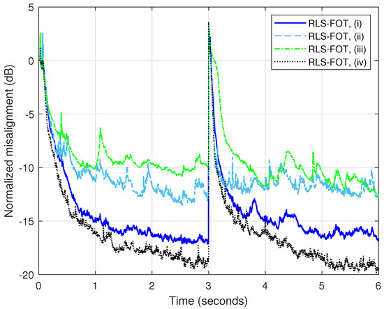
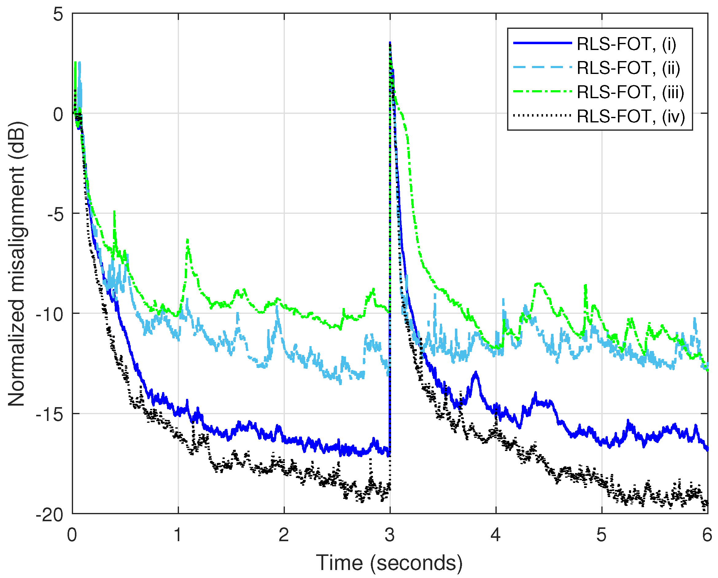
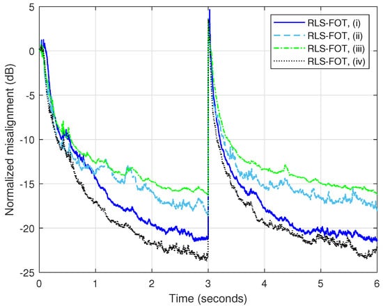
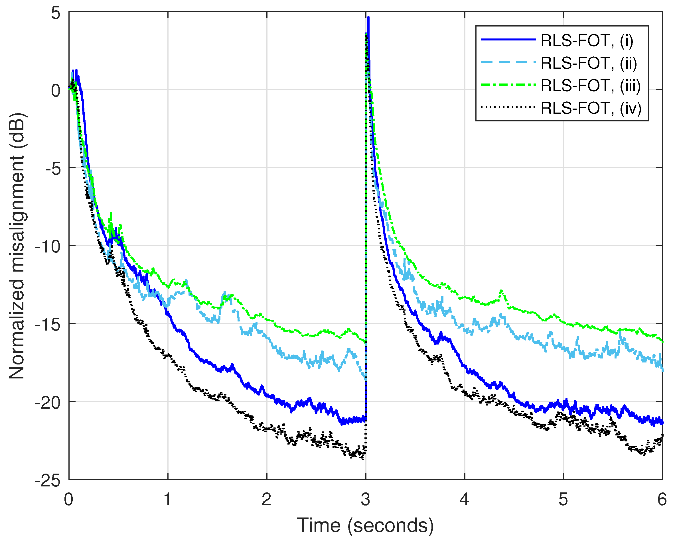
Using $P=Q=1$ within the RLS-FOT leads to a smaller parameter space and lower computational complexity, as outlined in Section 3, related to Figure 5, Figure 6 and Figure 7. In the first experiment, we evaluate this setup, considering the four decomposition scenarios mentioned in Section 3, i.e., (i)–(iv), and $R=L_{21}{L}_{22}/2$. The forgetting factors from (56)–(59) are computed using $\kappa =10$. The results are presented in Figure 8. Evidently, even when using $P=Q=1$, the RLS-FOT can lead to reasonable attenuation of misalignment (around $-15$ to $-20$ dB) for some decomposition scenarios, e.g., (i) and (iv). These two scenarios consider $L_1=L_2$ in the first step of the decomposition from (1), which is also the recommended choice in [26,27], where it is justified that these factors should be chosen as close as possible. Nevertheless, even low-complexity scenarios (ii) and (iii) reach below $-10$ dB in terms of misalignment.

Figure 8. Normalized misalignment of the RLS-FOT with $P=Q=1$ and $R=L_{21}{L}_{22}/2$ using $\kappa =10$ for computing the forgetting factors from (56)–(59) and different decomposition scenarios: (i) $L_{11}=8$, $L_{12}=4$, $L_{21}=8$, $L_{22}=4$, (ii) $L_{11}=16$, $L_{12}=4$, $L_{21}=4$, $L_{22}=4$, (iii) $L_{11}=8$, $L_{12}=8$, $L_{21}=4$, $L_{22}=4$, and (iv) $L_{11}=16$, $L_{12}=2$, $L_{21}=16$, $L_{22}=2$. The input signal is a speech sequence, $\mathrm{SNR}=20$ dB, and the AIR from Figure 2a changes after 3 s.

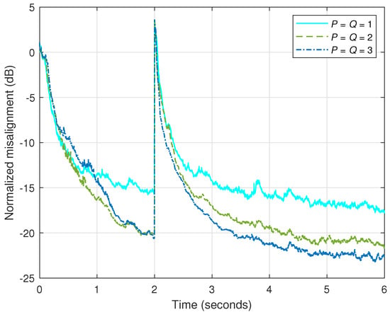
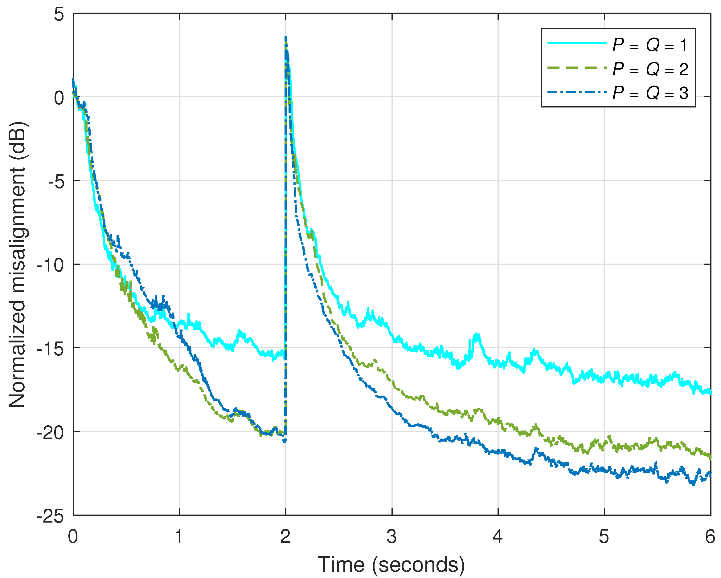
As expected, the performance can be improved by increasing the values of P and Q. This is justified in Figure 9, where $P=Q=2$, while the other conditions remain the same as in the previous experiment. It can be noticed that the misalignment level is lower (compared to Figure 8) for all the decomposition scenarios. This is further supported in Figure 10, where decomposition scenario (i) is considered, with different values of P and Q. In this context, it should also be noticed that the performance improvement is not significant after a certain threshold related to the values of P and Q, which is associated with the rank of the corresponding matrices, as explained in Section 2, related to Figure 4. Therefore, the setup $P=Q=2$ represents a proper compromise in terms of the main performance criteria. Naturally, the computational amount of the RLS-FOT is also larger when P and Q increase, as shown in Figure 7. However, this amount is below the complexity order of the conventional RLS algorithm.

Figure 9. Normalized misalignment of the RLS-FOT with $P=Q=2$ and $R=L_{21}{L}_{22}/2$ using $\kappa =10$ for computing the forgetting factors from (56)–(59) and different decomposition scenarios: (i) $L_{11}=8$, $L_{12}=4$, $L_{21}=8$, $L_{22}=4$, (ii) $L_{11}=16$, $L_{12}=4$, $L_{21}=4$, $L_{22}=4$, (iii) $L_{11}=8$, $L_{12}=8$, $L_{21}=4$, $L_{22}=4$, and (iv) $L_{11}=16$, $L_{12}=2$, $L_{21}=16$, $L_{22}=2$. The input signal is a speech sequence, $\mathrm{SNR}=20$ dB, and the AIR from Figure 2a changes after 3 s.

Figure 10. Normalized misalignment of the RLS-FOT (with $R=L_{21}{L}_{22}/2$) for different values of $P=Q$ using $\kappa =10$ for computing the forgetting factors from (56)–(59) and decomposition scenario (i): $L_{11}=8$, $L_{12}=4$, $L_{21}=8$, $L_{22}=4$. The input signal is a speech sequence, $\mathrm{SNR}=20$ dB, and the AIR from Figure 2a changes after 2 s.

Following the experiments from Figure 8, Figure 9 and Figure 10, the runtime of the RLS-FOT (expressed in milliseconds per iteration) is shown in Table 2, the values being obtained by averaging over 10 independent runs. These simulations were performed using MATLAB R2025b for programming, running on a GIGABYTE AORUS 15G XC device (Windows 11 OS), which has an Intel Core i7-10870H CPU with eight cores, 16 logical processors (@2.21 GHz base speed), and 32 GB of RAM. The same four decomposition scenarios are considered, i.e., (i)–(iv), together with different settings for the parameters P and Q (which have equal values). As expected, the runtime increases for larger values of P and Q, as also indicated in Figure 7 and Table 1 (in terms of computational complexity). Moreover, the runtime corresponding to the four analyzed scenarios follows the same hierarchy from Figure 7.

Table 2. Runtime of the RLS-FOT (in milliseconds per iteration) using different settings of the parameters $P=Q$ and $R=L_{21}{L}_{22}/2$ for decomposition scenarios (i)–(iv) from Figure 8, Figure 9 and Figure 10.

Settings	Scenario (i)	Scenario (ii)	Scenario (iii)	Scenario (iv)
$P=Q=1$	$5.394$	$2.795$	$2.218$	$7.365$
$P=Q=2$	$17.168$	$9.299$	$7.916$	$26.985$
$P=Q=3$	$38.003$	$18.602$	$15.672$	not applicable

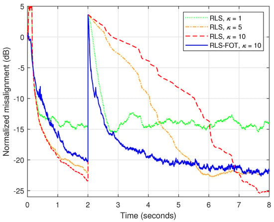
The forgetting factor is the main parameter of the conventional RLS algorithm, which controls its overall performance in terms of convergence/tracking and accuracy [1,2,3]. While the initial convergence rate is not relevant [10], the tracking capability of the algorithm is highly influenced by the forgetting factor. A larger value of $\lambda$ (or $\kappa$) from (55) leads to improved accuracy, i.e., lower misalignment. On the other hand, the tracking capability is affected due to the “heavier” memory of the algorithm, i.e., $\lambda$ being closer to one. Reducing the value of the forgetting factor (or the related parameter $\kappa$) acts in the opposite way, improving the tracking and sacrificing in terms of accuracy. Since the conventional RLS algorithm operates with a single (long-length) adaptive filter, this behavior is more apparent. Contrarily, the RLS-FOT combines four shorter adaptive filters (with individual forgetting factors), thus being more robust to this performance compromise. This aspect is supported in Figure 11, where the conventional RLS algorithm using different values of $\lambda$ from (55), which are tuned via the parameter $\kappa$, is compared with the RLS-FOT using $\kappa =10$ in (56)–(59) under the first decomposition scenario (i), with $P=Q=2$. As we can notice, the tracking capability of the RLS-FOT is similar to the conventional RLS algorithm using the lowest forgetting factor (with $\kappa =1$), but it achieves a lower misalignment level. Using a larger value of the forgetting factor (e.g., with $\kappa =10$) improves the accuracy of the conventional RLS algorithm but with a significantly slower tracking reaction. Nevertheless, the RLS-FOT also achieves reasonable attenuation of misalignment while demonstrating fast tracking behavior, thus leading to a better compromise in terms of these performance criteria. Moreover, the computational complexity of the RLS-FOT is lower compared to the conventional RLS benchmark, as shown in Figure 7 (in Section 3).

Figure 11. Normalized misalignment of the conventional RLS algorithm (with $L=1024$) using different values of $\kappa$ for computing the forgetting factor from (55) and the RLS-FOT (with $R=L_{21}{L}_{22}/2$ and $P=Q=2$) using $\kappa =10$ for computing the forgetting factors from (56)–(59), with decomposition scenario (i): $L_{11}=8$, $L_{12}=4$, $L_{21}=8$, $L_{22}=4$. The input signal is a speech sequence, $\mathrm{SNR}=20$ dB, and the AIR from Figure 2a changes after 2 s.

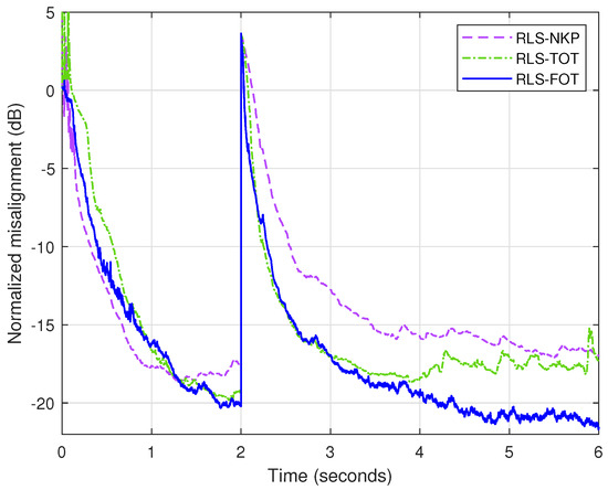
Next, the proposed RLS-FOT is compared to the previously developed tensor-based counterparts, i.e., RLS-NKP [27] and RLS-TOT [29], which exploit the second-order and third-order decompositions, respectively. The factorization of the RLS-NKP (i.e., $L=L_1{L}_2$) is performed using $L_1=L_2=32$, while the RLS-TOT uses $L_{11}^{\prime }=32$, $L_{12}^{\prime }=16$, and $L_2^{\prime }=2$ (i.e., $L=L_{11}^{\prime }{L}_{12}^{\prime }{L}_2^{\prime }$). The associated forgetting factors of these algorithms are evaluated based on (55) using the appropriate filters’ lengths and $\kappa =10$. Consequently, the RLS-NKP uses ${\lambda }_1=1-1/\left(\kappa R{L}_1\right)$ and ${\lambda }_2=1-1/\left(\kappa R{L}_2\right)$, with $R<L_2$. Also, the RLS-TOT involves ${\lambda }_{11}^{\prime }=1-1/\left(\kappa M{L}_{11}^{\prime }{L}_2^{\prime }\right)$, ${\lambda }_{12}^{\prime }=1-1/\left(\kappa M{L}_{12}^{\prime }{L}_2^{\prime }\right)$, and ${\lambda }_2^{\prime }=1$, with $M<L_{12}^{\prime }$. As shown in [29], the parameter ${\lambda }_2^{\prime }$ is associated with the shortest filter of RLS-TOT, with length $L_2^{\prime 2}=4$ coefficients; consequently, its forgetting factor can be set to its maximum value (one). In the experiment reported in Figure 12, the proposed RLS-FOT uses decomposition scenario (i), with $L_{11}=8$, $L_{12}=4$, $L_{21}=8$, $L_{22}=4$, together with $R=L_{21}{L}_{22}/2$ and $P=Q=2$. Based on the complexity order of the algorithms from Figure 7, the computational amount corresponding to the RLS-FOT (i) with $P=Q=2$ is slightly higher than the RLS-NKP using $R=8$ and RLS-TOT using $M=6$ (the two benchmarks have similar computational complexity under this setup). Consequently, these settings are also used in the comparison from Figure 12. As we can notice, the RLS-FOT outperforms both its decomposition-based counterparts, reaching a lower misalignment level, which reflects in better accuracy of the estimate.

Figure 12. Normalized misalignment of the RLS-NKP [27] (with $L_1=L_2=32$ and $R=8$), RLS-TOT (with $L_{11}^{\prime }=32$, $L_{12}^{\prime }=16$, $L_2^{\prime }=2$, and $M=6$), and RLS-FOT (with $L_{11}=8$, $L_{12}=4$, $L_{21}=8$, $L_{22}=4$, $R=L_{21}{L}_{22}/2$, and $P=Q=2$) using $\kappa =10$ for computing the forgetting factors based on (55). The input signal is a speech sequence, $\mathrm{SNR}=20$ dB, and the AIR from Figure 2a changes after 2 s.

Following the experiments from Figure 11 and Figure 12, the runtimes of the compared algorithms (expressed in milliseconds per iteration) are shown in Table 3, the values being obtained by averaging over 10 independent runs. These results validate the computational complexity hierarchy from Figure 7. As we can notice, the runtime corresponding to the conventional RLS algorithm is almost four times higher than the decomposition-based algorithms, as also indicated in Figure 7. Since the computational complexity of the RLS-FOT using $P=Q=2$ is slightly higher than its counterparts, i.e., RLS-NKP with $R=8$ and RLS-TOT with $M=6$ (as explained related to Figure 12), the runtime of the proposed algorithm is also slightly higher. In our simulations, we used MATLAB R2025b for programming. Clearly, the runtime depends on the simulation/implementation platform and the potential optimization procedures. For example, the operations related to the Kronecker product could be optimized [58,59], an approach that can be considered for further practical implementations of the decomposition-based algorithms.

Table 3. Runtime (in milliseconds per iteration) of the conventional RLS algorithm, RLS-NKP [27] (with $R=8$), RLS-TOT [29] (with $M=6$), and RLS-FOT (with $P=Q=2$ and $R=L_{21}{L}_{22}/2$) for the experimental scenarios from Figure 11 and Figure 12.

Algorithm	Runtime (Milliseconds/Iteration)
RLS	$61.668$
RLS-NKP [27]	$15.275$
RLS-TOT [29]	$15.524$
RLS-FOT	$16.946$

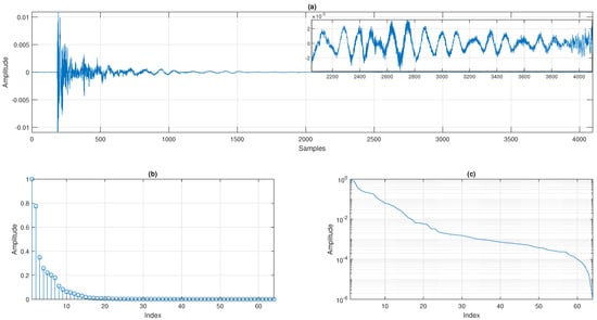
In the last experiment, a longer AIR is considered, as shown in Figure 13a. Its length is $L=4096$, with a sampling rate of 16 kHz. As explained in Section 2, this length can be factorized using $L_1=L_2=64$. The singular values of the corresponding matrix, $\mathbf{H}$, of size $64\times 64$ (obtained by reshaping this AIR) are depicted in Figure 13b,c using linear- and log-scale representations, respectively. It can be noticed that this AIR also has low-rank properties, while the approximated rank (R) is also lower than $L_2/2$, e.g., choosing the decision threshold in the range 0.001 to 0.01 at linear scale and ${10}^{-3}$ to ${10}^{-2}$ at log scale.

Figure 13. (a) Acoustic impulse response ($\mathbf{h}$) with $L=4096$ coefficients (using a sampling rate of 16 kHz) and $T_{60}=0.148$ s, where the top-right subplot shows a zoomed portion of its last $L/2$ coefficients. Singular values (normalized with respect to the maximum one) of the corresponding matrix, $\mathbf{H}$, of size $64\times 64$ using (b) linear representation and (c) log-scale representation.

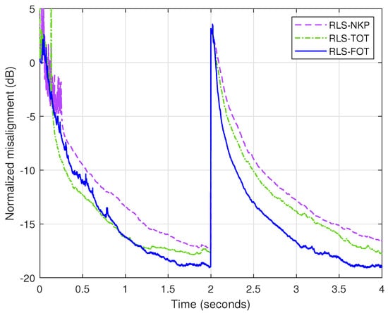
In Figure 14, the RLS-NKP [27], RLS-TOT, and RLS-FOT are compared, similar to the scenario from Figure 12. Nevertheless, the decomposition setup is different due to the higher length of the AIR. In this case, the RLS-NKP uses the factorization $L_1=L_2=64$, while the setup of the RLS-TOT involves $L_{11}^{\prime }=64$, $L_{12}^{\prime }=32$, $L_2^{\prime }=2$. The most natural factorization for the proposed RLS-FOT is $L_{11}=L_{12}=L_{21}=L_{22}=8$ while using $R=L_{21}{L}_{22}/2$ (as in the previous experiments). The other decomposition parameters are the same from Figure 12. As we can notice, the proposed RLS-FOT outperforms the other decomposition-based algorithms in terms of both convergence/tracking and accuracy of the estimate (i.e., misalignment level).

Figure 14. Normalized misalignment of the RLS-NKP [27] (with $L_1=L_2=64$ and $R=8$), RLS-TOT (with $L_{11}^{\prime }=64$, $L_{12}^{\prime }=32$, $L_2^{\prime }=2$, and $M=6$), and RLS-FOT (with $L_{11}=L_{12}=L_{21}=L_{22}=8$, $R=L_{21}{L}_{22}/2$, and $P=Q=2$) using $\kappa =10$ for computing the forgetting factors based on (55). The input signal is a speech sequence, the impulse response (of length $L=4096$) is the AIR from Figure 13a, $\mathrm{SNR}=20$ dB, and the AIR from Figure 13a changes after 2 s.

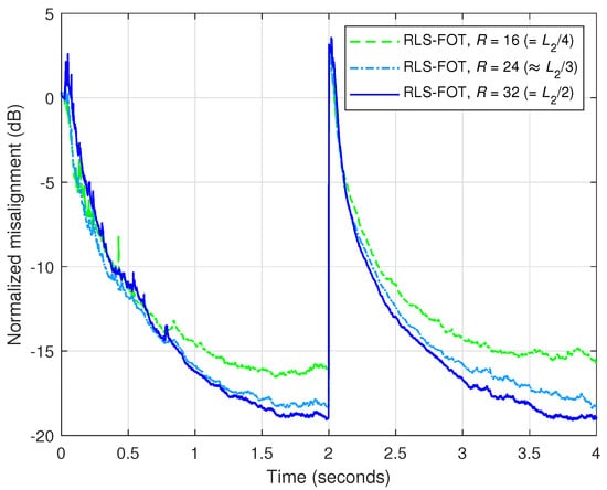
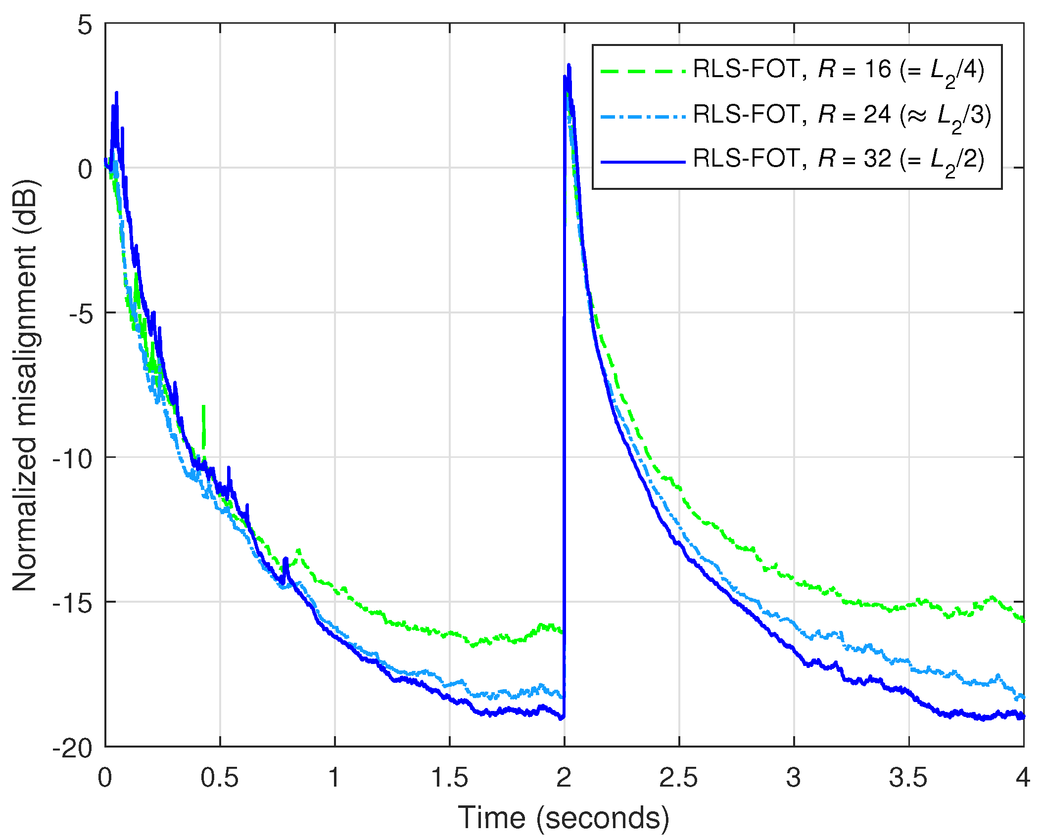
For such long-length AIRs, like in Figure 13a, the low-rank properties can be further exploited by using a lower value of R. As is evident from the singular value representation from Figure 13c, using a threshold between ${10}^{-2}$ and ${10}^{-3}$, the parameter R could be set in the range $L_2/4$ to $L_2/2$. Thus, in Figure 15, the performance of RLS-FOT is evaluated for different values of R within this interval. As expected, the misalignment increases for smaller values of R; however, it reaches below $-15$ dB even for $R=L_2/4$. While $R=L_2/2$ represents a practical choice when no a priori information about the AIR is available, as outlined before in Section 3, the value of this decomposition parameter could be set even lower in some scenarios (e.g., with known room characteristics), also saving in terms of computational complexity, as indicated in Table 1.

Figure 15. Normalized misalignment of the RLS-FOT using different values of R (in the range $L_2/4$ to $L_2/2$), $P=Q=2$, and $\kappa =10$ for computing the forgetting factors from (56)–(59), for the identification of the AIR from Figure 13a, with $L=4096$ and the factorization setup $L_{11}=L_{12}=L_{21}=L_{22}=8$ (i.e., $L_1=L_2=64$). The input signal is a speech sequence, $\mathrm{SNR}=20$ dB, and the AIR from Figure 13a changes after 2 s.

5. Conclusions and Perspectives

The decomposition of the impulse response is an appealing technique in system identification problems, especially when dealing with long-length AIRs, which possess low-rank characteristics. Such an approach fits very well in the context of AEC, where the length of the adaptive filter can reach hundreds/thousands of coefficients. In this paper, we have developed an RLS-type algorithm that exploits a fourth-order tensor decomposition. As a result, the proposed RLS-FOT combines the coefficients of four shorter adaptive filters (using the Kronecker product) compared to the conventional RLS solution, which relies on a single long-length filter. The advantage is twofold in terms of both performance and complexity. The RLS-FOT achieves a better performance compromise in terms of the main criteria (i.e., tracking versus accuracy) compared to the conventional RLS algorithm. Also, the proposed algorithm has lower computational complexity, which can be adjusted by using a proper factorization of the impulse response. Moreover, for the same complexity order, the RLS-FOT outperforms its previously developed counterparts that rely on second-order and third-order decompositions, i.e., the RLS-NKP [27] and RLS-TOT [29]. The simulation results obtained in the framework of AEC indicate the good performance features of the RLS-FOT, which could be a potential choice for real-world AEC scenarios. The experimental evaluation presented in this paper involves measured AIRs and recorded speech signals, with the main goal of outlining the potential gains of the proposed algorithm. An important objective for future work is to test the RLS-FOT in a real-world application scenario.

There are several pending challenges related to the proposed RLS-FOT. First, rank selection (i.e., the setup for parameters R, P, and Q) remains an open issue. Even if their values can be set in practice based on some recommended choices (as explained at the end of Section 3), it would be highly useful to find a more rigorous way to determine these parameters. Nevertheless, this is not a straightforward task since the system to be identified is not available in real-time applications, while only some intrinsic characteristics (e.g., sparsity, reflections, etc.) could be exploited. A potential solution would be to set these parameters based on an estimate of the filter impulse response, which could be available after the initial convergence phase. In other words, a conventional adaptive filter could be used for the initial convergence, followed by switching to the decomposition-based algorithm, with the rank-related parameters set based on the available estimate of the impulse response. On the other hand, the system could change in practice since, in echo cancellation, we deal with time-varying echo paths, so the impulse response characteristics (and the associated parameters) should also be reassessed. Moreover, in noisy environments, the initial convergence of the algorithm and its steady-state estimate are more problematic, which further influences the accuracy of the solution. Second, regarding the robustness of the algorithm in noisy conditions, a regularized version of the RLS-FOT would be of interest, as briefly explained at the end of this section.

In perspective, a higher order of the decomposition will be analyzed, taking into account that the tensor rank should be controlled and limited to a known value. In addition, more computationally efficient techniques for solving the normal equations of the algorithm will be analyzed, like those that exploit line search methods [7,10]. These would further facilitate the practical implementation of the algorithm on DSP and/or FPGA platforms. In order to improve the performance balance between tracking and accuracy, a version of the RLS-FOT with variable forgetting factors can be further developed, aiming for better control of these convergence parameters. Finally, the cost functions of the algorithm can be equipped with specific regularization terms, which could improve overall robustness in noisy environments. Naturally, the overall performance of any adaptive filtering algorithm is affected in noisy conditions, which especially reflects in reducing the accuracy of the estimate. In the case of RLS-type algorithms, using only the forgetting factors as the control parameters leads to inherent performance limitations. Therefore, the cost functions should include (besides the error-based terms) additional regularization components that contain appropriate parameters related to background noise and model uncertainties.

References

- Sayed, A.H. Adaptive Filters; Wiley: New York, NY, USA, 2008. [Google Scholar]
- Haykin, S. Adaptive Filter Theory, 4th ed.; Pearson: Upper Saddle River, NJ, USA, 2014. [Google Scholar]
- Diniz, P.S.R. Adaptive Filtering: Algorithms and Practical Implementation, 5th ed.; Springer Nature: Cham, Switzerland, 2020. [Google Scholar]
- Benesty, J.; Huang, Y. (Eds.) Adaptive Signal Processing–Applications to Real-World Problems; Springer: Berlin, Germany, 2003. [Google Scholar]
- Hänsler, E.; Schmidt, G. Acoustic Echo and Noise Control–A Practical Approach; Wiley: Hoboken, NJ, USA, 2004. [Google Scholar]
- Zakharov, Y.V.; Tozer, T.C. Multiplication-free iterative algorithm for LS problem. IEE Electron. Lett. 2004, 40, 567–569. [Google Scholar] [CrossRef] [Scilit]
- Zakharov, Y.V.; White, G.P.; Liu, J. Low-complexity RLS algorithms using dichotomous coordinate descent iterations. IEEE Trans. Signal Process. 2008, 56, 3150–3161. [Google Scholar] [CrossRef] [Scilit]
- Apolinário, J.A., Jr. (Ed.) QRD-RLS Adaptive Filtering; Springer: New York, NY, USA, 2009. [Google Scholar]
- Liu, J.; Zakharov, Y.V.; Weaver, B. Architecture and FPGA design of dichotomous coordinate descent algorithms. IEEE Trans. Circuits Syst. I Regul. Pap. 2009, 56, 2425–2438. [Google Scholar]
- Zakharov, Y.V.; Nascimento, V.H. DCD-RLS adaptive filters with penalties for sparse identification. IEEE Trans. Signal Process. 2013, 61, 3198–3213. [Google Scholar] [CrossRef] [Scilit]
- Yu, Y.; Lu, L.; Zheng, Z.; Wang, W.; Zakharov, Y.; de Lamare, R.C. DCD-based recursive adaptive algorithms robust against impulsive noise. IEEE Trans. Circuits Syst. II Express Briefs 2020, 67, 1359–1363. [Google Scholar] [CrossRef] [Scilit]
- Van Loan, C.F. The ubiquitous Kronecker product. J. Comput. Appl. Math. 2000, 123, 85–100. [Google Scholar] [CrossRef] [Scilit]
- Salmi, J.; Richter, A.; Koivunen, V. Sequential unfolding SVD for tensors with applications in array signal processing. IEEE Trans. Signal Process. 2009, 57, 4719–4733. [Google Scholar] [CrossRef] [Scilit]
- Vervliet, N.; Debals, O.; Sorber, L.; De Lathauwer, L. Breaking the curse of dimensionality using decompositions of incomplete tensors: Tensor-based scientific computing in big data analysis. IEEE Signal Process. Mag. 2014, 31, 71–79. [Google Scholar] [CrossRef] [Scilit]
- Rupp, M.; Schwarz, S. A tensor LMS algorithm. In Proceedings IEEE International Conference on Acoustics, Speech, and Signal Processing (ICASSP); IEEE: New York, NY, USA, 2015; pp. 3347–3351. [Google Scholar]
- Rupp, M.; Schwarz, S. Gradient-based approaches to learn tensor products. In Proceedings European Signal Processing Conference (EUSIPCO); IEEE: New York, NY, USA, 2015; pp. 2486–2490. [Google Scholar]
- Ribeiro, L.N.; de Almeida, A.L.F.; Mota, J.C.M. Identification of separable systems using trilinear filtering. In Proceedings IEEE International Workshop on Computational Advances in Multi-Sensor Adaptive Processing (CAMSAP); IEEE: New York, NY, USA, 2015; pp. 189–192. [Google Scholar]
- Friedland, S.; Tammali, V. Low-rank approximation of tensors. In Numerical Algebra, Matrix Theory, Differential-Algebraic Equations and Control Theory; Benner, P., Bollhöfer, M., Kressner, D., Mehl, C., Stykel, T., Eds.; Springer: Cham, Switzerland, 2015; pp. 377–411. [Google Scholar]
- Cichocki, A.; Mandic, D.P.; Phan, A.; Caiafa, C.F.; Zhou, G.; Zhao, Q.; De Lathauwer, L. Tensor decompositions for signal processing applications: From two-way to multiway component analysis. IEEE Signal Process. Mag. 2015, 32, 145–163. [Google Scholar] [CrossRef] [Scilit]
- Becker, H.; Albera, L.; Comon, P.; Gribonval, R.; Wendling, F.; Merlet, I. Brain-source imaging: From sparse to tensor models. IEEE Signal Process. Mag. 2015, 32, 100–112. [Google Scholar] [CrossRef] [Scilit]
- Bousse, M.; Debals, O.; Lathauwer, L.D. A tensor-based method for large-scale blind source separation using segmentation. IEEE Trans. Signal Process. 2017, 65, 346–358. [Google Scholar] [CrossRef] [Scilit]
- Sidiropoulos, N.; Lathauwer, L.D.; Fu, X.; Huang, K.; Papalexakis, E.; Faloutsos, C. Tensor decomposition for signal processing and machine learning. IEEE Trans. Signal Process. 2017, 65, 3551–3582. [Google Scholar] [CrossRef] [Scilit]
- Ribeiro, L.N.; Schwarz, S.; Rupp, M.; de Almeida, A.L.F.; Mota, J.C.M. A low-complexity equalizer for massive MIMO systems based on array separability. In Proceedings European Signal Processing Conference (EUSIPCO); IEEE: New York, NY, USA, 2017; pp. 2522–2526. [Google Scholar]
- da Costa, M.N.; Favier, G.; Romano, J.M.T. Tensor modelling of MIMO communication systems with performance analysis and Kronecker receivers. Signal Process. 2018, 145, 304–316. [Google Scholar] [CrossRef] [Scilit]
- Ribeiro, L.N.; de Almeida, A.L.F.; Mota, J.C.M. Separable linearly constrained minimum variance beamformers. Signal Process. 2019, 158, 15–25. [Google Scholar] [CrossRef] [Scilit]
- Paleologu, C.; Benesty, J.; Ciochină, S. Linear system identification based on a Kronecker product decomposition. IEEE/ACM Trans. Audio Speech Lang. Process. 2018, 26, 1793–1808. [Google Scholar] [CrossRef] [Scilit]
- Elisei-Iliescu, C.; Paleologu, C.; Benesty, J.; Stanciu, C.; Anghel, C.; Ciochină, S. Recursive least-squares algorithms for the identification of low-rank systems. IEEE/ACM Trans. Audio Speech Lang. Process. 2019, 27, 903–918. [Google Scholar] [CrossRef] [Scilit]
- Benesty, J.; Paleologu, C.; Ciochină, S. Linear system identification based on a third-order tensor decomposition. IEEE Signal Process. Lett. 2023, 30, 503–507. [Google Scholar] [CrossRef] [Scilit]
- Paleologu, C.; Benesty, J.; Stanciu, C.L.; Jensen, J.R.; Christensen, M.G.; Ciochină, S. Recursive least-squares algorithm based on a third-order tensor decomposition for low-rank system identification. Signal Process. 2023, 213, 109216. [Google Scholar] [CrossRef] [Scilit]
- Golub, G.H.; Van Loan, C.F. Matrix Computations, 3rd ed.; The John Hopkins University Press: Baltimore, MD, USA, 1996. [Google Scholar]
- Hansen, P.C. Rank-Deficient and Discrete Ill-Posed Problems: Numerical Aspects of Linear Inversion; SIAM: Philadelphia, PA, USA, 1998. [Google Scholar]
- Kolda, T.G.; Bader, B.W. Tensor decompositions and applications. SIAM Rev. 2009, 51, 455–500. [Google Scholar] [CrossRef] [Scilit]
- Comon, P. Tensors: A brief introduction. IEEE Signal Processing Mag. 2014, 31, 44–53. [Google Scholar] [CrossRef] [Scilit]
- Bhattacharjee, S.S.; George, N.V. Nearest Kronecker product decomposition based normalized least mean square algorithm. In Proceedings IEEE International Conference on Acoustics, Speech, and Signal Processing (ICASSP); IEEE: New York, NY, USA, 2020; pp. 476–480. [Google Scholar]
- Bhattacharjee, S.S.; George, N.V. Fast and efficient acoustic feedback cancellation based on low rank approximation. Signal Process. 2021, 182, 107984. [Google Scholar] [CrossRef] [Scilit]
- Bhattacharjee, S.S.; George, N.V. Nearest Kronecker product decomposition based linear-in-the-parameters nonlinear filters. IEEE/ACM Trans. Audio Speech Lang. Process. 2021, 29, 2111–2122. [Google Scholar] [CrossRef] [Scilit]
- Bhattacharjee, S.S.; Patel, V.; George, N.V. Nonlinear spline adaptive filters based on a low rank approximation. Signal Process. 2022, 201, 108726. [Google Scholar] [CrossRef] [Scilit]
- Vadhvana, S.; Yadav, S.K.; Bhattacharjee, S.S.; George, N.V. An improved constrained LMS algorithm for fast adaptive beamforming based on a low rank approximation. IEEE Trans. Circuits Syst. II Express Briefs 2022, 69, 3605–3609. [Google Scholar] [CrossRef] [Scilit]
- Dehghan, M.; de M. Goulart, J.H.; de Almeida, A.L.F. Low-rank multilinear filtering. Digit. Signal Process. 2024, 153, 104646. [Google Scholar] [CrossRef] [Scilit]
- Wang, Z.; Zhu, Z.; Zeng, X.; He, H.; Yu, Y.; Yang, T. A third-order tensor decomposition approach for adaptive speech dereverberation. In INTER-NOISE and NOISE-CON Congress and Conference Proceedings; Institute of Noise Control Engineering: Wakefield, MA, USA, 2025; pp. 1402–1412. [Google Scholar]
- Ye, J.; Zhao, H. Nearest Kronecker product decomposition based subband adaptive filter: Algorithms and applications. IEEE Trans. Audio Speech Lang. Process. 2026, 34, 691–706. [Google Scholar] [CrossRef] [Scilit]
- Zhu, Y.; Huang, G.; Jin, J.; Chen, J.; Benesty, J. A third-order tensor decomposition based algorithm for speech dereverberation. Signal Process. 2026, 239, 110210. [Google Scholar] [CrossRef] [Scilit]
- Frank, J.S.A.; Cohen, I.; George, N.V. Generalized sidelobe canceller for time-domain region-of-interest beamforming. IEEE Trans. Audio Speech Lang. Process. 2026, 34, 878–894. [Google Scholar]
- Zhao, K.; Jin, J.; Luo, X.; Huang, G.; Chen, J.; Benesty, J. Design of low-rank differential beamformers with constrained directivity or robustness. Signal Process. 2026, 243, 110487. [Google Scholar] [CrossRef] [Scilit]
- Ghosh, S.; Meena, T.; George, N.V. Low-rank enhanced Hammerstein-spline adaptive filter for sparsity-aware nonlinear feedback cancellation in hearing aids. Signal Process. 2026, 244, 110518. [Google Scholar] [CrossRef] [Scilit]
- International Telecommunication Union. Digital Network Echo Cancellers; ITU-T Recommendation G.168; International Telecommunication Union (ITU): Geneva, Switzerland, 2015.
- Benesty, J.; Paleologu, C.; Dogariu, L.M. An iterative Wiener filter based on a fourth-order tensor decomposition. Symmetry 2023, 15, 1560. [Google Scholar] [CrossRef] [Scilit]
- Duttweiler, D.L. Proportionate normalized least-mean-squares adaptation in echo cancelers. IEEE Trans. Speech Audio Process. 2000, 8, 508–518. [Google Scholar] [CrossRef] [Scilit]
- Bertsekas, D.P. Nonlinear Programming, 2nd ed.; Athena Scientific: Belmont, MA, USA, 1999. [Google Scholar]
- Zhou, N.; Trudnowski, D.J.; Pierre, J.W.; Mittelstadt, W.A. Electromechanical mode online estimation using regularized robust RLS methods. IEEE Trans. Power Syst. 2008, 23, 1670–1680. [Google Scholar] [CrossRef] [Scilit]
- Eksioglu, E.M.; Tanc, A.K. RLS algorithm with convex regularization. IEEE Signal Process. Lett. 2011, 18, 470–473. [Google Scholar] [CrossRef] [Scilit]
- Iqbal, N.; Zerguine, A. AFD-DFE using constraint-based RLS and phase noise compensation for uplink SC-FDMA. IEEE Trans. Veh. Technol. 2017, 66, 4435–4443. [Google Scholar] [CrossRef]
- Yang, F.; Yang, J.; Albu, F. An alternative solution to the dynamically regularized RLS algorithm. In 2019 Asia-Pacific Signal and Information Processing Association Annual Summit and Conference (APSIPA ASC); IEEE: New York, NY, USA, 2019; pp. 1072–1075. [Google Scholar]
- Lawal, A.; Abed-Meraim, K.; Mayyala, Q.; Iqbal, N.; Zerguine, A. Blind adaptive channel estimation using structure subspace tracking. In 2021 55th Asilomar Conference on Signals, Systems, and Computers; IEEE: New York, NY, USA, 2021; pp. 1372–1376. [Google Scholar]
- Li, B.; Wu, S.; Tripp, E.E.; Pezeshki, A.; Tarokh, V. Recursive least squares with minimax concave penalty regularization for adaptive system identification. IEEE Access 2024, 12, 66993–67004. [Google Scholar] [CrossRef] [Scilit]
- Zhong, Y.; Yu, C.; Xiang, X.; Lian, L. Proximal policy-optimized regularized least squares algorithm for noise-resilient motion prediction of UMVs. IEEE J. Ocean. Eng. 2024, 49, 1397–1410. [Google Scholar] [CrossRef] [Scilit]
- Otopeleanu, R.A.; Benesty, J.; Paleologu, C.; Stanciu, C.L.; Dogariu, L.M.; Ciochină, S. A practical regularized recursive least-squares algorithm for robust system identification. In 2025 33rd European Signal Processing Conference (EUSIPCO); IEEE: New York, NY, USA, 2025; pp. 1417–1421. [Google Scholar]
- Tadonki, C. Large scale Kronecker product on supercomputers. In Proceedings Workshop on Architecture and Multi-Core Applications (WAMCA); IEEE: New York, NY, USA, 2011; pp. 1–4. [Google Scholar]
- Azevedo, A.; Bentes, C.; Castro, M.C.; Tadonki, C. Performance analysis and optimization of the vector-Kronecker product multiplication. In Proceedings IEEE International Symposium on Computer Architecture and High Performance Computing (SBAC-PAD); IEEE: New York, NY, USA, 2020; pp. 265–272. [Google Scholar]
Disclaimer/Publisher’s Note: The statements, opinions and data contained in all publications are solely those of the individual author(s) and contributor(s) and not of MDPI and/or the editor(s). MDPI and/or the editor(s) disclaim responsibility for any injury to people or property resulting from any ideas, methods, instructions or products referred to in the content. |
© 2026 by the authors. Licensee MDPI, Basel, Switzerland. This article is an open access article distributed under the terms and conditions of the Creative Commons Attribution (CC BY) license.