Frequency-Based Deep Occlusion Awareness Instance Segmentation

Abstract

One major challenge faced by deep learning-based methods that detect target objects in the form of bounding boxes is object occlusion. High degrees of occlusion significantly diminish the accuracy of instance segmentation. Nonetheless, complex-valued Fourier descriptors can robustly represent object boundaries using minimal information. In this study, the impact of integrating Fourier descriptors—renowned for their strong representational capacity—with deep network models (UNet) that exhibit high generalization performance on instance segmentation accuracy was investigated. Within the scope of the research, nine network models were designed based on different strategies for utilizing frequency components. These variants fall into four strategy families: (i) UNet-style spectrum regression on fixed low-frequency windows (FUNet), (ii) magnitude-guided frequency selection/ROI construction (FUNet–Thr, FUNet–BBox), (iii) sequence models over tokenized FFT coefficients (BiLSTM Patch/Sorted), and (iv) encoder-only spectrum predictors with different depth/capacity (EncoderFFT1/2). To fairly evaluate the models’ performance in segmenting objects subjected to disruptive factors (e.g., occlusion, blurring, noise), a specialized synthetic dataset was prepared. The task is formulated as single-target (single-instance), single-class segmentation. This dataset, automatically generated according to initial parameter values, contains images of objects moving at various speeds within a single frame. Among these models, the one termed FUNet, which relies on partial matching of central frequency components, achieved the highest segmentation accuracy despite the disruptive effects. Under the challenging Dataset 8 setting, the proposed FUNet achieved the highest overlap-based performance (Dice = 0.9329, IoU = 0.8842) among Attention U-Net, U-Net, and FourierNet, with statistically significant gains confirmed by paired per-image tests.

1. Introduction

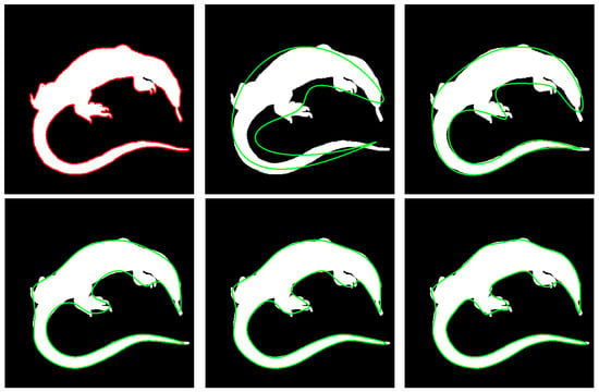
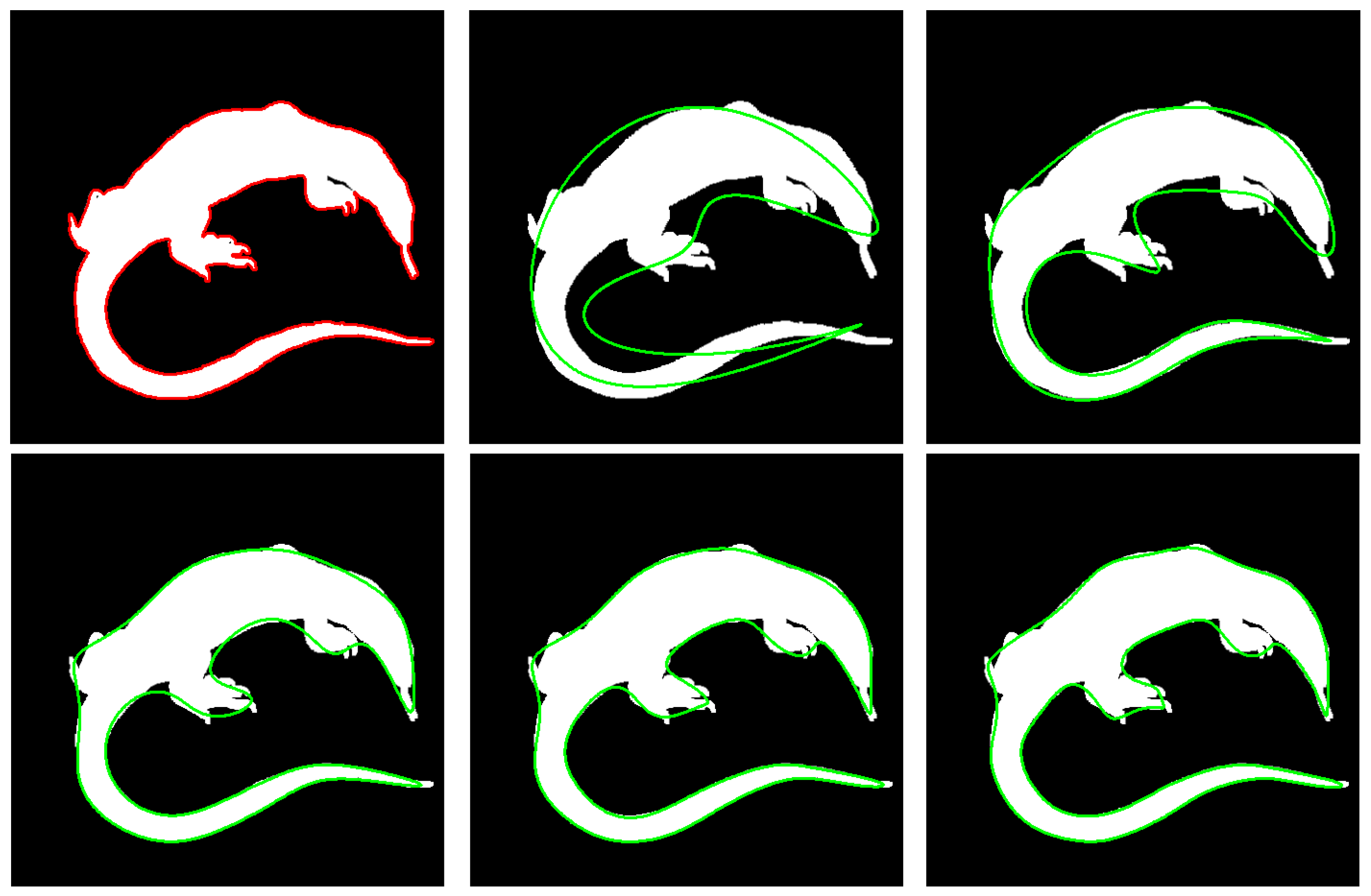
It is well established that object geometries can be robustly represented with minimal information using General Fourier Descriptors (GFD) [1]. In contrast to conventional contour- and region-based approaches in the spatial domain, GFD’s ability to effectively capture high-dimensional edge information with a limited number of complex Fourier components—and to flexibly adjust the number of these components—has made it an attractive method for researchers. To better illustrate this representational power, Figure 1 presents an example image of a lizard alongside its red-colored edges and the reconstruction results (in green) using varying numbers of frequency components. The spatial-domain edge information for this $446\times 446$ image measures $2090\times 2$. After performing the spatial-frequency transformation, reconstruction using only the first 10, 20, 30, 40, and 50 frequency components, respectively, produces the green edge representations shown. As the results indicate, around 30 complex frequency components suffice to capture the lizard’s complex geometry at an adequate level.

Figure 1. Representation of an object’s geometric shape using General Fourier Descriptors. The first image displays the original lizard object, with its boundary shown in red. The subsequent images illustrate the reconstructed boundaries (in green), obtained by applying inverse transformations using 10, 20, 30, 40, and 50 GFD coefficients, respectively.

Segmentation is the process of dividing an image into meaningful segments by assigning each pixel to its corresponding object or region [2]. This procedure is critical for identifying object boundaries and distinguishing different regions within the image [3]. It plays a fundamental role in numerous fields, including medical image analysis, autonomous vehicles, face recognition, satellite imaging, and industrial quality control [4]. By reducing image complexity and highlighting relevant information, segmentation enables more efficient and accurate analysis [5]. In particular, deep learning-based methods enhance both the speed and accuracy of this process, catering to a wide range of applications [6].

Single-stage and two-stage instance segmentation are two fundamental approaches commonly utilized for object detection and segmentation [7]. In the single-stage approach, detection and segmentation are carried out simultaneously within a single network, offering a rapid and efficient process [5,8]. In contrast, the two-stage approach first identifies object candidates, followed by a more precise segmentation of those candidates [9]. Although it generally requires slower inference speeds, increased computational complexity, and additional training steps, this approach often yields higher accuracy and finer detail [10]. Mask R-CNN is one of the most prominent examples of two-stage segmentation, delivering high accuracy by producing pixel-level, refined masks for detected objects [11].

Classical image segmentation methods provide effective and straightforward solutions in scenarios with limited data and computational resources [12]. Techniques such as thresholding and clustering (e.g., K-means) group pixels based on intensity, color, or texture, while region growing and edge-based techniques (e.g., Canny or Sobel) delineate object boundaries [4]. Graph cut separates foreground and background by leveraging energy minimization principles, whereas the watershed method confines regions using a water-basin analogy [13,14]. Owing to their simplicity and low computational cost, these methods remain in use; however, they exhibit limited performance in complex and dynamic scenes when compared to modern deep learning techniques [12].

Deep learning-based segmentation methods leverage powerful neural networks to classify pixels, thereby delivering revolutionary contributions to modern image processing [6]. Convolutional Neural Networks (CNNs) and architectures such as UNet offer detailed and precise segmentation, while methods like Mask R-CNN and DeepLab stand out for their object detection and learning capabilities [11,15,16]. These approaches provide high accuracy and efficiency in various domains, including medical imaging, autonomous vehicles, and satellite analysis, surpassing traditional techniques. The limited generalization performance of classical segmentation approaches, contrasted with the robust generalization exhibited by deep learning models trained on large datasets, has rapidly positioned deep learning solutions as the dominant approach in the field of segmentation [12].

CNN-based networks commonly employ an encoder-decoder architecture that filters spatial information from images [12]. In this framework, the encoder extracts features by encoding the image into low-dimensional representations, while the decoder utilizes these features to reconstruct a high-resolution output, generating the segmentation mask in the process [15]. Because objects’ distinguishing characteristics may occur in any part of the image, convolutional filters are applied across all image regions during model training. In high-resolution images or when working with large-scale datasets, the computational cost of sliding these filters increases considerably [12]. Consequently, researchers have been motivated to develop more cost-effective models and to explore methods that require reduced computational resources.

As illustrated in Equation (1), the convolution operation in the spatial domain is equivalent to pointwise multiplication in the frequency domain.

$$\mathcal{F}\left\{f\right(r,c)\ast g(r,c\left)\right\}(u,v)=F(u,v)·G(u,v)$$

(1)

Here, $\mathcal{F}\{·\}$ denotes the 2-D discrete Fourier transform (DFT), $f(r,c)$ is the input image at spatial coordinates $(r,c)$, $g(r,c)$ is the convolution kernel, and ∗ denotes 2-D convolution. $F(u,v)=\mathcal{F}\left\{f\right\}(u,v)$ and $G(u,v)=\mathcal{F}\left\{g\right\}(u,v)$ are the corresponding frequency-domain representations, where $(u,v)$ denote frequency indices and “·” denotes pointwise multiplication.

A small example can be provided to better illustrate the computational costs of convolution in the spatial domain versus multiplication in the frequency domain. Let the input image be of size $N\times N$ and the convolution kernel be of size $K\times K$.

$$C_{\mathrm{spatial}}\approx N^2{K}^2,C_{\mathrm{spatial}}\in O\left(N^2{K}^2\right).$$

(2)

For $N=1000$ and $K=9$, the operation count is approximately

$C_{\mathrm{spatial}}\approx {1000}^2·9^2=81\times {10}^6$.

$$C_{\mathrm{freq}}\approx 2N^2{log}_{2}N+N^2,C_{\mathrm{freq}}\in O\left(N^{2}logN\right).$$

(3)

The factor 2 accounts for the forward 2-D FFT and the inverse 2-D FFT, and the $N^2$ term corresponds to pointwise multiplication in the frequency domain. For $N=1000$, ${log}_2\left(1000\right)\approx 9.97$, hence

$$C_{\mathrm{freq}}\approx 2·{10}^6·9.97+{10}^6\approx 2.093\times {10}^7\approx 21\times {10}^6$$

Even though the frequency-domain cost encompasses the sum of transformation (spatial-to-frequency and frequency-to-spatial) and multiplication, it is still approximately four times lower than the spatial convolution cost. Moreover, for higher-dimensional masks, this discrepancy becomes even more pronounced. This advantage constitutes one of the primary reasons researchers opt for frequency-domain approaches.

When an image is transformed from the spatial domain to the frequency domain (see Equation (4)), its content can be expressed as a sum of sinusoids with varying amplitude and phase information [2]. Each sinusoid in the frequency domain (corresponding to one pixel in that domain) maps back to an image in the spatial domain. Low-frequency sinusoids capture the overall patterns and geometric structure of the image, whereas high-frequency sinusoids encapsulate fine details and rapid variations [17]. Decomposing image content into these distinct sinusoidal components is particularly advantageous for isolating objects with different patterns and textures.

$$F(u,v)={\displaystyle \frac{1}{RC}}\sum _{r=0}^{R-1}\sum _{c=0}^{C-1}f(r,c)e^{-i2\pi \left({\displaystyle \frac{ur}{R}}+{\displaystyle \frac{vc}{C}}\right)}$$

(4)

where $f(r,c)$ denotes the spatial-domain image with R rows and C columns. Spatial indices satisfy $r\in \{0,\dots ,R-1\}$ and $c\in \{0,\dots ,C-1\}$, while $(u,v)$ denote frequency indices with $u\in \{0,\dots ,R-1\}$ and $v\in \{0,\dots ,C-1\}$. The DFT coefficients $F(u,v)$ are complex-valued, and $i=\sqrt{-1}$ denotes the imaginary unit. The normalization factor $1/\left(RC\right)$ follows the adopted DFT convention.

A second major advantage of leveraging frequency-domain information is its relative independence from spatial manipulations such as scaling (enlargement or reduction), translation, and rotation of an object [2]. This characteristic arises from the frequency domain’s capacity to represent global properties. For example, altering an object’s size merely compresses or stretches the frequencies in the frequency spectrum. Similarly, shifting an object’s spatial position does not affect the amplitude spectrum; instead, it introduces a phase shift. Rotations, meanwhile, rotate the frequency spectrum but preserve the amplitude distribution. These properties enable easier detection of objects exhibiting different scales, positions, and orientations in the frequency domain [17].

Frequency-domain analysis can demonstrate greater robustness against occlusion— situations in which one object is partially or completely covered by another—[18]. Occlusion represents a significant challenge in segmentation, particularly in the spatial domain where overlapping objects complicate accurate boundary delineation [19]. Because the overall pattern of an object shares the same characteristics as a small portion of its pattern, the sinusoids corresponding to a partially occluded object can still be detected through frequency transformation. In this regard, using frequency-domain information for object detection offers a substantial advantage.

Despite the strong performance of spatial-domain encoder–decoder segmentation models, their pixel-wise decoding can degrade notably under severe occlusion and common image degradations (e.g., noise and blur), where only partial visual evidence of the target object is available. In contrast, frequency-domain representations provide a global and compact characterization of image structure, and low-frequency components can preserve coarse shape information even when local details are corrupted. Motivated by these observations, an investigation is conducted into whether learning a direct mapping from the complex FFT representation of an input image to the complex FFT representation of its target mask can yield more robust instance segmentation in occlusion-heavy settings. To address this gap, a frequency-domain instance segmentation framework is proposed, and its robustness is benchmarked under controlled occlusion and degradations.

The main contributions of this work are: (1) A fully frequency-domain instance segmentation pipeline is proposed that predicts the target mask’s FFT coefficients and performs spatial reconstruction only once via inverse FFT at inference time, enabling direct learning over frequency components. (2) A systematic comparison of nine frequency-domain model variants is conducted, including partial matching and frequency-selection strategies, to identify design choices that most improve robustness. (3) An evaluation protocol is introduced on a newly generated single-target synthetic benchmark with controllable occlusion, noise, and blur, and results are reported against strong baselines (UNet and FourierNet) to assess robustness in challenging settings.

2. Related Work

This section reviews segmentation studies that leverage frequency-domain information. A first line of work uses Fourier series or Fourier descriptors to obtain compact, shape-aware mask representations. Riaz et al. [7] proposed FourierNet, a low-parameter and fast method that estimates Fourier coefficients along with classification scores, centerness, and a bounding box to construct object masks. By employing a differentiable shape decoder, the method refines masks and exploits the high information content of low-frequency components, supporting both polar and Cartesian coordinate systems. Cansiz et al. [20] introduced a model based on Fourier descriptors for segmenting the Henle Fiber Layer (HFL) in standard OCT images; the approach learns shape priors and predicts both Fourier-descriptor maps and the corresponding segmentation map. Similarly, Jeon et al. [21] introduced FCSN, which estimates Fourier coefficients to generate segmentation masks while preserving global context, improving shape topology, and maintaining robustness against local distortions with lower computational cost than conventional encoder–decoder designs.

A second line of work incorporates frequency-domain transforms into the segmentation pipeline to improve efficiency or preserve fine details. Khan et al. [22] integrated the Fast Fourier Transform (FFT) into active contour models, enabling faster and more accurate salient-object detection (particularly in medical and synthetic images) without requiring contour re-initialization. For remote sensing, Liu et al. [23] proposed AFCNet, which combines a UNet backbone with a Fourier Neural Encoder to capture both fine road details and long-range road continuity. Xu et al. [24] explored training segmentation models directly on frequency components obtained via the Discrete Cosine Transform (DCT) instead of spatial-domain down-sampling; by selecting the most informative frequency channels, redundant components are removed while using mask images as outputs.

Recent studies have continued to exploit frequency-domain representations to improve robustness and shape faithfulness in segmentation. Pham et al. [25] proposed FFTMed, a lightweight U-shaped architecture operating directly in the Fourier domain for medical image segmentation. Erden et al. [26] introduced FourierLoss, a shape-aware loss that penalizes discrepancies between Fourier-descriptor-based shape characterizations of the ground truth and predicted segmentation maps. Le et al. [27] proposed CamoFA, a learnable Fourier-based augmentation strategy that mixes low- and high-frequency components to boost camouflage detection and instance segmentation performance. Fourier-guided instance segmentation in weakly supervised settings has also been investigated (FrGNet) [28], and frequency-aware encoder–decoder designs integrating spectral modeling and frequency-informed objectives have been reported (FreqU-FNet) [29].

Prior frequency-aware segmentation studies typically (i) use Fourier descriptors as auxiliary shape priors or additional losses while still predicting masks in the spatial domain, or (ii) parameterize object boundaries with a small set of Fourier coefficients coupled with detection components (e.g., bounding boxes/centerness) as in FourierNet-like designs. In contrast, this work formulates segmentation as a direct frequency-to-frequency learning problem: the network regresses the complex FFT coefficients of the target mask (within a controlled low-frequency window) from the FFT representation of the input image, and the final mask is obtained via inverse FFT. Beyond proposing this formulation, the study provides a structured comparison of nine frequency-domain strategies (frequency-window selection, magnitude-guided token/ROI selection, partial matching of central components, and sequence/encoder backbones) under controlled occlusion and degradations on a single-target synthetic benchmark. This systematic taxonomy and robustness-focused evaluation constitute the main novelty relative to prior Fourier-prior and Fourier-descriptor segmentation approaches.

3. Generation of the Synthetic Segmentation Dataset

In order to evaluate the performance of the segmentation methods developed in this study and to provide a versatile resource for future research, a specialized synthetic dataset was created. The dataset was generated in a simulation environment where ten distinct objects independently move, rotate, and scale on a two-dimensional surface. Each image has a resolution of $512\times 512$ pixels. To introduce varying levels of complexity, the dataset was organized into 16 distinct difficulty levels, each comprising 1000 images.

The simulation process is structured into two main stages based on object interaction behaviors. Collision Stage: In this stage, objects change their direction upon collision. As a result, significant occlusion between objects is minimized, leading to clearer object boundaries. This setup simulates environments where object interactions prevent substantial overlapping, and it is particularly suitable for studies focusing on relatively occlusion-free segmentation tasks. Collision-Free Stage: In contrast, during this stage, objects continue their movement trajectories without altering their paths even when overlaps occur. Consequently, objects frequently occlude one another, creating complex visual scenes with significant object overlaps. During ground-truth generation for this stage, complete object masks are preserved, ensuring that each object’s full geometric structure is annotated, regardless of its visibility in the rendered image. The inclusion of both stages was intentional to enhance the dataset’s applicability to a broad range of segmentation challenges. While the Collision Stage provides cleaner scenarios with minimal occlusion, the Collision-Free Stage offers complex occlusion cases that mirror real-world conditions more accurately.

Furthermore, each main stage is subdivided into eight sub-stages, incorporating various image processing techniques and background manipulations to simulate different environmental complexities:

1.

Stage 1 (Basic Level): In this stage, objects move randomly on a black background without introducing any additional complexity.

2.

Stage 2 (Colored Background): In this stage, the background colors of the images vary. These colors are generated using different characteristic values defined in the HSV color space.

3.

Stage 3 (Noise Addition): In this stage, while the background remains black, Gaussian noise is applied to each image, thereby distorting the appearance of the objects. The Gaussian noise is defined with a mean value of 0 and a variance of 0.05.

4.

Stage 4 (Blur Addition): The background remains black; however, in this stage, the entire image is blurred. The blurring process is performed using a kernel size of 9 × 9 with a standard deviation of 0.

5.

Stage 5 (Colored Background and Noise Addition): In this stage, the background colors vary according to the HSV color space as in Stage 2, and Gaussian noise is additionally applied to each image.

6.

Stage 6 (Colored Background and Blur Addition): In this stage, the background colors vary and a blurring effect is applied to the images.

7.

Stage 7 (Noise and Blur Addition): In this stage, with the background remaining black, both Gaussian noise and a blurring effect are applied to the images.

8.

Stage 8 (Colored Background, Noise, and Blur Addition): In this most complex stage, the background color varies and each image is subjected to both noise and blur effects. This stage represents the highest difficulty level in the synthetic dataset.

Synthetic corruption model: Let $x\in {\mathbb{R}}^{H\times W\times C}$ denote a clean image and y the synthetically corrupted image. Additive Gaussian noise is modeled as

$$y=x+n,n_{i,j,k}\sim \mathcal{N}(0,{\sigma }_n^2),$$

(5)

where ${\sigma }_n$ denotes the noise standard deviation. Gaussian blur is modeled by convolution with a Gaussian kernel

$$y=x\ast g,g(u,v)={\displaystyle \frac{1}{2\pi {\sigma }_b^2}}exp\left(-{\displaystyle \frac{u^2+v^2}{2{\sigma }_b^2}}\right),$$

(6)

where ∗ denotes discrete convolution and g is a normalized 2-D Gaussian blur kernel parameterized by the blur standard deviation ${\sigma }_b$, i.e., ${\sum }_{u,v}g(u,v)=1$ (in practice, g is truncated to a finite kernel size). The combined corruption used in the synthetic dataset (Gaussian blur followed by additive Gaussian noise) is

$$y=(x\ast g)+n.$$

(7)

The values (or ranges) of ${\sigma }_n$ and ${\sigma }_b$ are set according to the experimental settings reported in this study.

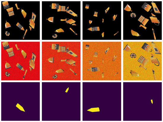
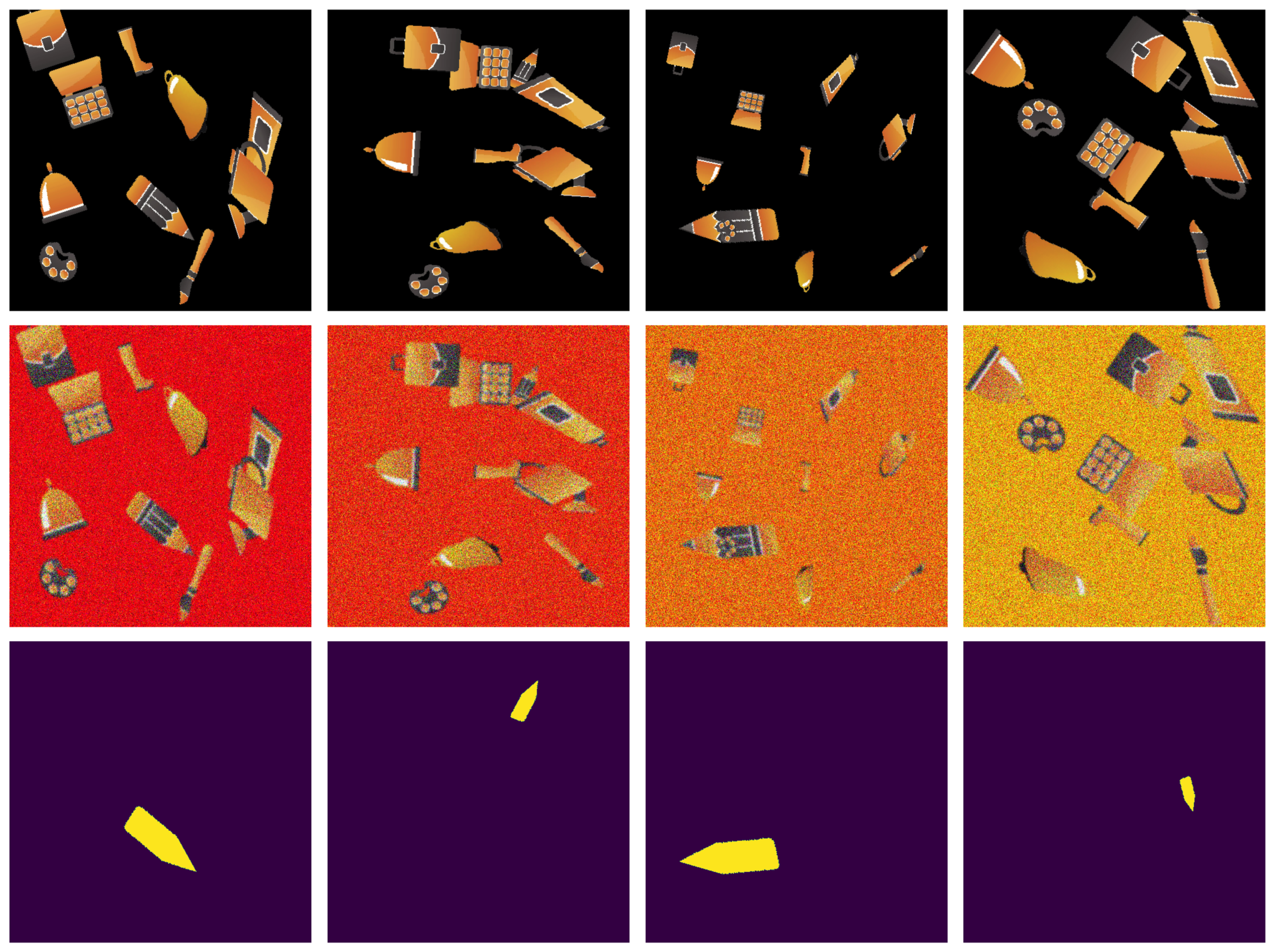
Dataset protocol: In this work, to comprehensively address the occlusion problem and assess the resilience of the frequency domain under noisy conditions, we utilized the collision-free dataset, specifically selecting images from Stage 1 and Stage 8 (see Figure 2). Stage 1 and Stage 8 form paired samples derived from the same underlying simulation frames. First, a base set of clean frames is rendered (Stage 1). Stage 8 is then generated by applying synthetic corruptions (Gaussian blur and additive Gaussian noise) to the same frames, while keeping the ground-truth target mask unchanged. Accordingly, Stage 1 and Stage 8 share identical sample identifiers (file names) and the same target mask; only the input image differs due to corruption. For learning and evaluation, the dataset is split into train/validation/test subsets with a ratio of 70/15/15 (i.e., 700/150/150 samples, based on unique file identifiers). Crucially, splitting is performed once over these identifiers and the same partition is applied to both stages, ensuring that a given sample (clean/corrupted pair) appears in exactly one of train/validation/test (no cross-split leakage). Since each identifier corresponds to a unique simulation frame (and its underlying motion parameters), the trajectories associated with the samples are disjoint across train/validation/test. All stochastic components are controlled via fixed random seeds for reproducibility: Python (ver. 3.10) random and NumPy (ver. 1.26) are both set to 42 for generation/corruption, and the split is also generated using seed 42. Training is carried out separately for Stage 1 and Stage 8: a model is trained using the training split of the corresponding stage and tuned on its validation split, and performance is reported on the associated test split.

Figure 2. Synthetic dataset samples: (1st row)—noise-free images from Stage 1, (2nd row)—noisy images from Stage 8, (3rd row)—masks of the pencil object.

4. Proposed Frequency-Based Model and Approaches

In this section, the proposed models and methodologies are detailed. Two alternative target representations are considered: (a) predicting the mask in the frequency domain by regressing its complex spectrum $\mathcal{F}\left(m\right)$, and (b) predicting the binary mask directly in the spatial domain. For the frequency-domain formulation, both the input image x and the target mask m are transformed into the frequency domain using the Fast Fourier Transform (FFT). In this domain, the models are trained to predict the mask spectrum, i.e., $\widehat{\mathcal{F}\left(m\right)}$, and the training loss is computed directly between $\widehat{\mathcal{F}\left(m\right)}$ and the ground-truth $\mathcal{F}\left(m\right)$. During inference, test images—unseen during training—are likewise projected into the frequency domain, and the trained models predict $\widehat{\mathcal{F}\left(m\right)}$. The predicted spectrum is then reconstructed in the spatial domain by applying the Inverse Fast Fourier Transform (IFFT). For evaluation, the reconstructed output is binarized using a fixed threshold ($T=122$ on the $[0,255]$ scale) to produce the final segmentation mask. For the spatial-domain baseline (UNet), the model predicts the mask directly with a sigmoid output and is binarized at 0.5. Since Fourier reconstruction approximates sharp boundaries with a finite set of frequency components, partial-frequency settings can lead to mild Gibbs-like ringing near edges; thus, binarization can affect boundary crispness, and a fixed threshold is used consistently across FFT-based evaluations.

The model architecture utilized standard convolutional layers with default kernel sizes (typically 3 × 3), and the Adam optimizer was employed for training. The learning rate was set to its default value of 0.001, and the batch size was chosen as 4 based on memory constraints and empirical stability during training. All models were trained and evaluated using the same fixed train/validation/test split. Training was run for up to 200 epochs with early stopping (patience = 20) based on the validation performance. Alternative strategies aimed at improving training dynamics and convergence have also been explored in the literature (e.g., Lv et al. [30]).

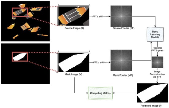
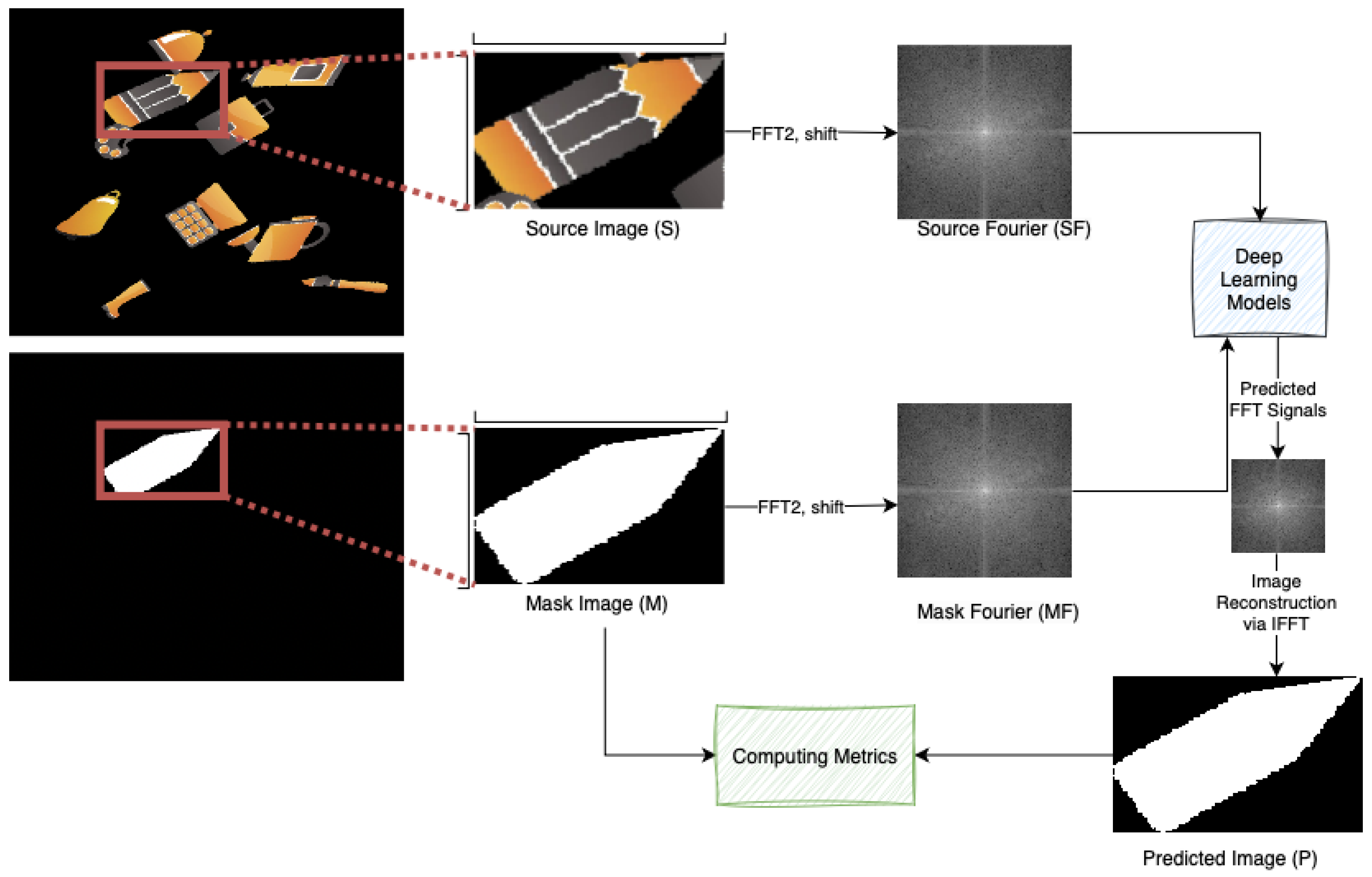
Performance evaluation was conducted by comparing the reconstructed masks with the ground truth annotations using standard metrics, including Precision, Recall [31], Dice Coefficient [32], and Intersection over Union (IoU) [33]. An overview of the entire pipeline is illustrated in Figure 3, providing a visual representation of the key processing steps, including frequency domain transformation, model inference, reconstruction, and evaluation.

Figure 3. Workflow of the proposed frequency-domain segmentation approach.

4.1. FUNet

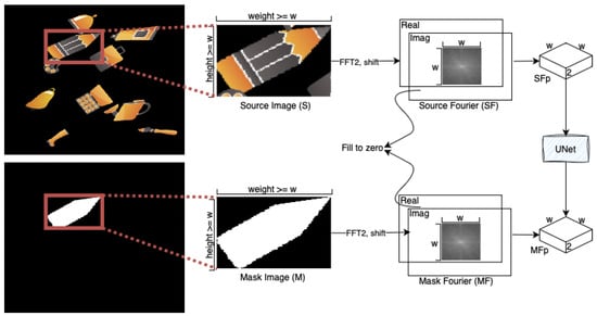
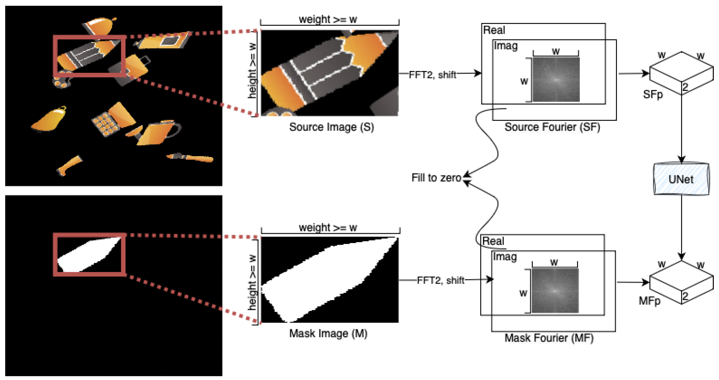
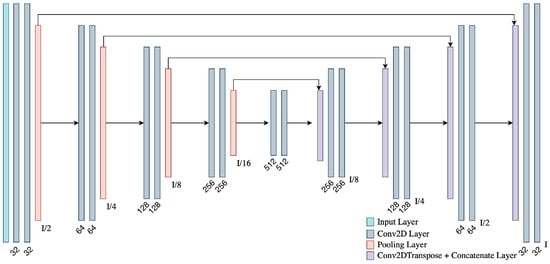
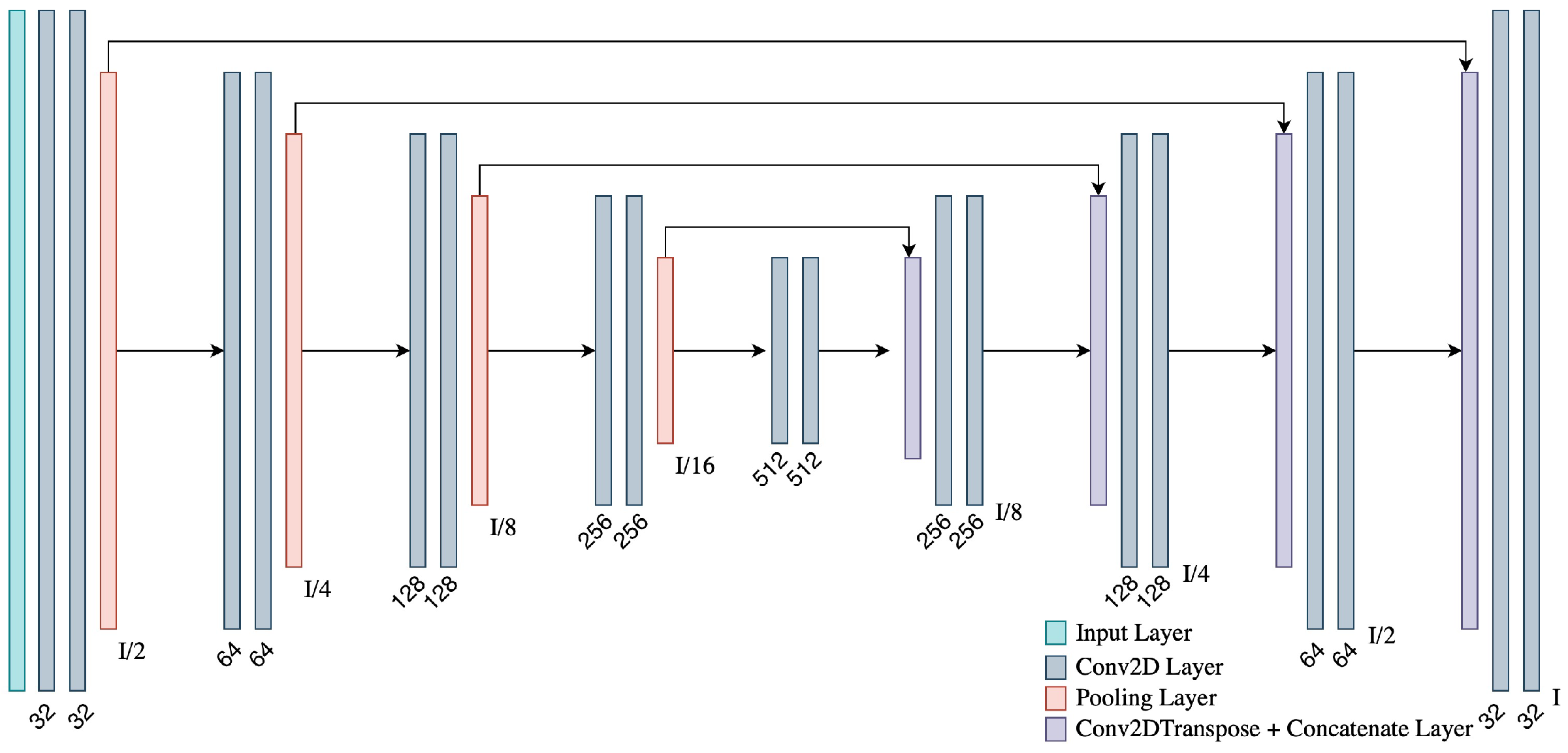
In this model, each image and its corresponding label from the dataset is first read. The images are then transformed into the frequency domain using the FFT2 command, and the low frequencies are repositioned to the center by applying the FFTShift command. Subsequently, small patches of dimensions $w\times w\times 2$ are extracted from the centers of the images (see Figure 4). A standard UNet [15] architecture illustrated in Figure 5 is trained using this dataset, which is prepared without any vectorization. To determine the optimal window size $\left(w\right)$ that maximizes segmentation performance, training and testing were repeated using window sizes of 16, 32, and 64.

Figure 4. Overall System Architecture.

Figure 5. The Architecture of UNet.

4.2. FUNet–Thr

The primary difference between this model and the FUNet model is the additional processing step applied after the images are transformed into the frequency domain via the Fast Fourier Transform (FFT). Following the transformation, the frequency-domain representation is denoted by the complex-valued matrix $F(u,v)$. Its real and imaginary parts are written as $\Re \left\{F\right(u,v\left)\right\}$ and $\Im \left\{F\right(u,v\left)\right\}$, respectively, with $i=\sqrt{-1}$. A magnitude matrix $M(u,v)$ is computed to represent the amplitude of each frequency component:

$$M(u,v)=\left|F(u,v)\right|=\sqrt{\Re {\left\{F(u,v)\right\}}^2+\Im {\left\{F(u,v)\right\}}^2}.$$

(8)

Subsequently, positions corresponding to frequency components whose magnitudes exceed a certain threshold are selected. Around each selected position, central tensors of size $w\times w\times 2$ are extracted to form the inputs for training the UNet model. These tensors contain both the real and imaginary parts of the original frequency domain representation. During training, the model receives the thresholded tensors as input and predicts the corresponding unthresholded tensors of the same dimensions. The threshold value for magnitude selection was treated as a hyperparameter, optimized through experiments with values of 0.01, 0.02, and 0.03.

4.3. FUNet-BBox

In this model, the input images are first transformed into the frequency domain using the Fast Fourier Transform (FFT), and the magnitude matrix $M(u,v)$ is computed as defined in Equation (8). A threshold is then applied to the magnitude matrix to retain significant frequency components. Unlike previous approaches, instead of selecting localized patches around thresholded points, a fixed window of size $160\times 160\times 2$ is chosen to encompass all the retained frequency signals within each image. This tensor, containing both real and imaginary components, serves as both the input and output during training. The threshold value for magnitude selection was treated as a hyperparameter and optimized by testing values of 0.01, 0.02, and 0.03.

4.4. LSTM-Based Models

LSTM models are primarily designed to operate on sequential data, as they can leverage backward contextual information to generate more accurate subsequent predictions. In segmentation tasks, however, spatial dependencies are crucial; that is, understanding the relationships between adjacent regions of an image can enhance performance. Consequently, this study investigates the impact of partitioning input images into segments, enabling the LSTM model to learn inter-segment dependencies on segmentation performance.

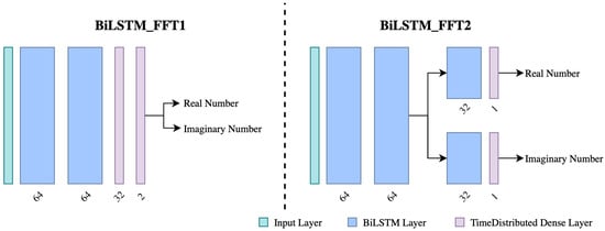
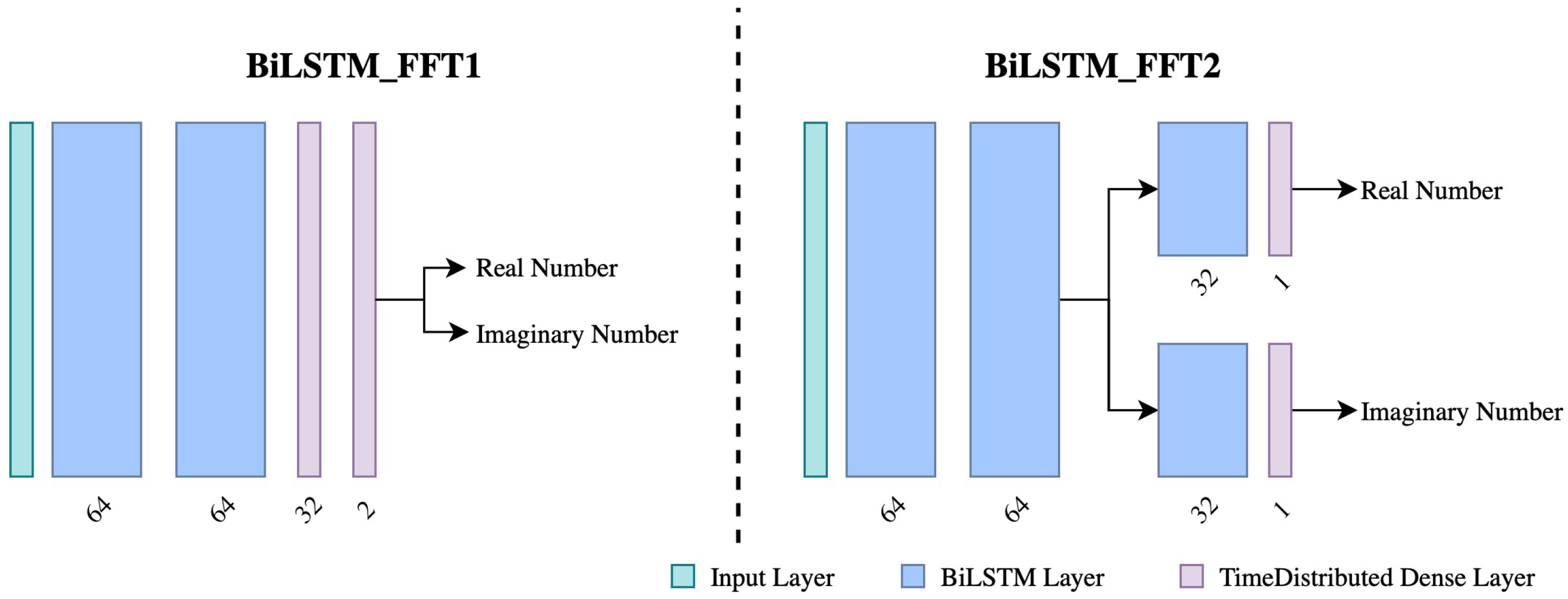
In both models, the input is a token sequence derived from the FFT coefficients (see LSTM-Patch and LSTM-Sorted below). The sequence is processed by stacked BiLSTM layers to produce a per-token prediction of the target mask spectrum (real and imaginary components). In Figure 6, the teal bar at the far left denotes the input sequence. The two large blue blocks labeled “64” represent two stacked BiLSTM layers with 64 units each. The purple blocks denote time-distributed dense layers applied to each token.

Figure 6. Architectures of LSTM-based models.

In this section, two distinct LSTM models are introduced, with their architectures depicted in Figure 6: BiLSTM_FFT1 (left) and BiLSTM_FFT2 (right).

BiLSTM_FFT1 after the two shared BiLSTM(64) layers, the model uses a time-distributed dense layer with 32 units (purple block labeled “32”), followed by a final time-distributed dense layer with 2 units (purple block labeled “2”) to jointly output the real and imaginary parts for each token.

BiLSTM_FFT2 after the same two shared BiLSTM(64) layers, the network splits into two parallel branches (upper: real, lower: imaginary). Each branch contains an additional BiLSTM layer with 32 units (blue block labeled “32”) and a final time-distributed dense layer with 1 unit (purple block labeled “1”) to predict the real or imaginary component separately.

4.4.1. LSTM-Patch

In this approach, after applying FFT to the input images and masks, the central $w\times w\times 2$ region is extracted (real/imag channels) and reshaped into a sequence of length $w^2$ with 2 features per token, i.e., an input of size $(w^2,2)$. The corresponding mask spectrum coefficients are used as the target sequence with the same shape. This sequence pair is used to train BiLSTM_FFT1 and BiLSTM_FFT2.

4.4.2. LSTM-Sorted

In this approach, each FFT coefficient is represented as a token with five attributes: row index, column index, real part, imaginary part, and magnitude, forming an input matrix of size $(w^2,5)$ after selecting the top $w^2$ coefficients sorted by magnitude. Using the selected $(u,v)$ locations, the corresponding mask-spectrum coefficients (real/imag) are gathered to form the target matrix of size $(w^2,2)$. These input–target sequences are then used to train BiLSTM_FFT1 and BiLSTM_FFT2.

4.5. Encoder Based Models

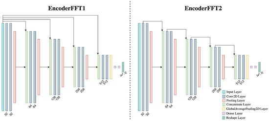
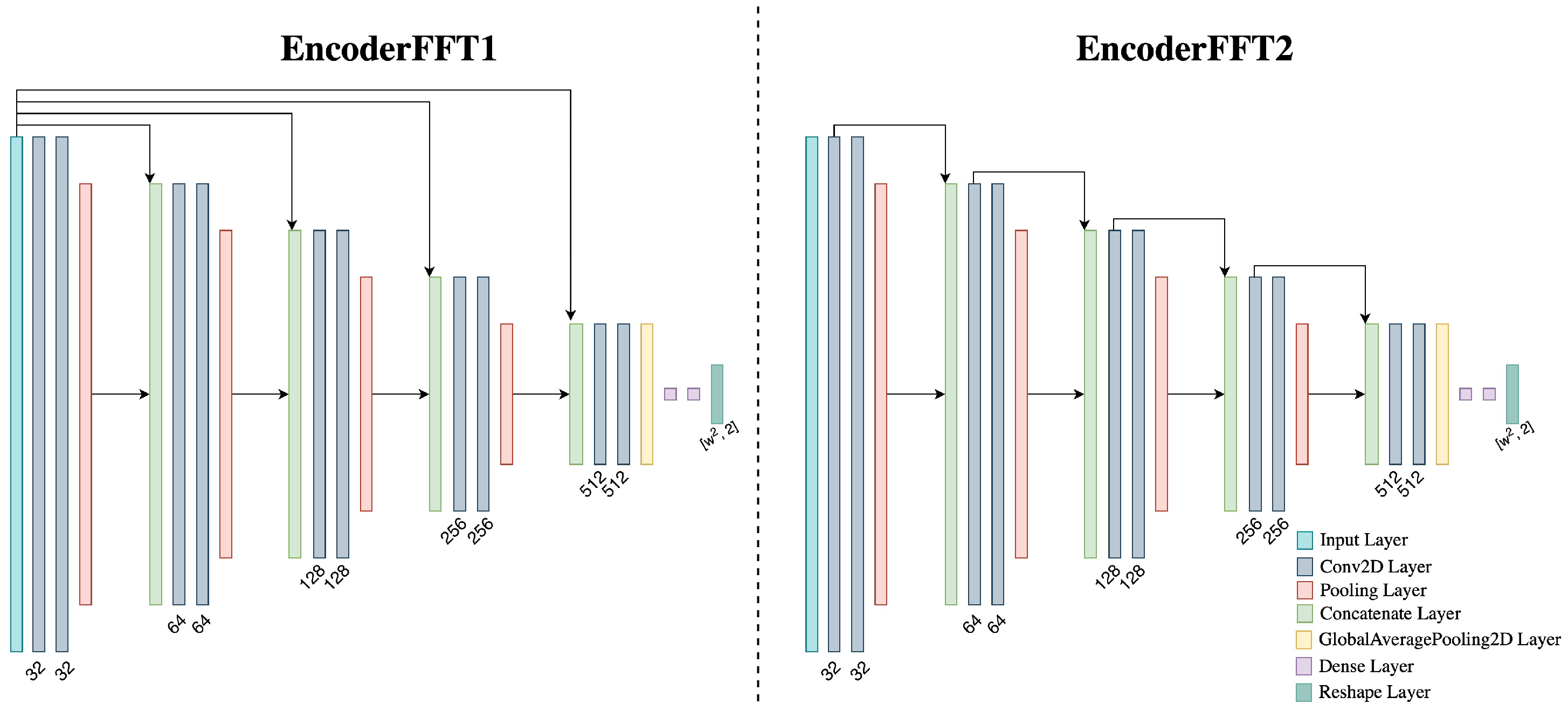
In this section, we present the EncoderFFT models depicted in Figure 7, which adopt an encoder-based architecture inspired by the encoder component of UNet. Unlike conventional segmentation models, the bottleneck of our approach is designed to predict frequency-domain representations of the target data. Specifically, after computing the FFT transformations of both the input images and the corresponding segmentation masks, the central $w\times w\times 2$ region of the resulting tensors is extracted. The FFT-transformed mask is then reshaped into a $w^2\times 2$ matrix, which serves as the target output during training. Simultaneously, the $w\times w\times 2$ FFT feature from the input image is provided to the encoder network. The key idea is that, by training the encoder to reconstruct the frequency domain of the mask, we can later apply an inverse FFT (IFFT) operation on the predicted output to obtain the final segmentation map, effectively delegating the decoding step to the IFFT process.

Figure 7. Architectures of Encoder-based models.

4.5.1. EncoderFFT1

Figure 7(left) shows EncoderFFT1, an encoder-only CNN that regresses the target mask spectrum from the input image spectrum. After FFT, the central $w\times w\times 2$ window (real/imag channels) is fed to stacked Conv2D blocks with pooling (increasing widths 32→64→128→256→512). Multi-scale features are fused via long skip connections and concatenation. The final representation is global-average pooled and mapped by Dense layers to $w^2\times 2$ outputs, which are reshaped to form $\widehat{\mathcal{F}\left(m\right)}$.

4.5.2. EncoderFFT2

Figure 7(right) shows EncoderFFT2, which uses the same input/output interface and encoder backbone, but changes the fusion topology: instead of long-range multi-scale skips, it applies stage-wise (block-aligned) concatenation between adjacent levels. The pooled encoder features are again projected with Dense layers and reshaped to obtain the predicted spectrum $\widehat{\mathcal{F}\left(m\right)}$.

5. Results

The performance of the developed models on Dataset 1 and Dataset 8 is presented in Table 1. The results indicate a significant decline in the performance of all models on Dataset 8, which is a substantially more challenging version of Dataset 1. For the best UNet-style frequency model, FUNet ($w=32$), Dice decreases from 0.9583 to 0.9329 (absolute drop 0.0254, ≈2.7% relative), while IoU decreases from 0.9237 to 0.8842 (drop 0.0395). In contrast, the drop is larger for FUNet-BBox (Dice: 0.9490→0.9110, drop 0.0380) and for the BiLSTM-Sorted variants (e.g., BiLSTM_FFT1_Sorted Dice: 0.8327→0.7599, drop 0.0728), indicating higher sensitivity to corruption in sequence-based tokenization.

Table 1. Evaluation results of the developed models.

	Dataset 1				Dataset 8
Model Name	Prec.	Recall	DiceC	IoU	Prec.	Recall	DiceC	IoU
FUNet ($w=32$)	0.9706	0.9472	0.9583	0.9237	0.9511	0.9170	0.9329	0.8842
FUNet-Thr ($w=32$, $T=0.01$)	0.9695	0.9417	0.9547	0.9171	0.9510	0.9108	0.9297	0.8797
FUNet-BBox ($w=160$, $T=0.01$)	0.9692	0.9309	0.9490	0.9055	0.9440	0.8833	0.9110	0.8483
BiLSTM_FFT1_Patch ($w=16$)	0.0460	0.0002	0.0003	0.0002	0.0448	0.0002	0.0004	0.0002
BiLSTM_FFT2_Patch ($w=16$)	0.0455	0.0002	0.0004	0.0002	0.0450	0.0002	0.0004	0.0002
BiLSTM_FFT1_Sorted ($w=64$)	0.8660	0.8107	0.8327	0.7208	0.7377	0.8045	0.7599	0.6244
BiLSTM_FFT2_Sorted ($w=16$)	0.8470	0.8394	0.8389	0.7286	0.7498	0.7826	0.7542	0.6184
EncoderFFT1 ($w=32$)	0.9592	0.9139	0.9347	0.8826	0.9425	0.8810	0.9083	0.8453
EncoderFFT2 ($w=32$)	0.9665	0.9211	0.9420	0.8938	0.9363	0.8921	0.9128	0.8508

Abbreviations: Prec.—Precision, DiceC—Dice Coefficient, IoU—Intersection Over Union. Note: Underlined values indicate the best score for each metric.

Among the nine developed variants, the UNet-based models achieve the highest overlap-based scores (Dice/IoU) on both datasets. In particular, FUNet ($w=32$) attains the best Dice and IoU on Dataset 1 (Dice = 0.9583, IoU = 0.9237) and remains the top-performing model on Dataset 8 (Dice = 0.9329, IoU = 0.8842). FUNet-Thr shows slightly lower Dice/IoU than FUNet on both datasets, while FUNet-BBox yields the largest drop within the FUNet variants on Dataset 8 (Dice = 0.9110, IoU = 0.8483).

The LSTM-based models exhibit substantially lower performance than the convolutional frequency-domain variants. The Patch-based BiLSTM models (BiLSTM_FFT1_Patch and BiLSTM_FFT2_Patch) produce near-zero overlap scores on both datasets, whereas the Sorted variants yield moderate performance (e.g., BiLSTM_FFT1_Sorted Dice = 0.8327 on Dataset 1 and 0.7599 on Dataset 8). Encoder-based variants (EncoderFFT1/2) are consistently stronger than the LSTM variants but remain below the FUNet family on Dataset 8 (EncoderFFT2 Dice = 0.9128, IoU = 0.8508).

Table 2 summarizes the performance of FUNet and the comparison other deep learning models on Dataset 1 and Dataset 8. Overall, FUNet ($w=32$) achieves the best overlap-based performance on both datasets. On Dataset 1, FUNet attains the highest precision (0.9706), Dice coefficient (0.9583), and IoU (0.9237), while Attention U-Net yields the highest recall (0.9664). In this cleaner setting, Attention U-Net and UNet also perform competitively (Dice: 0.9581 and 0.9564, respectively), whereas FourierNet shows noticeably lower overlap scores (Dice: 0.9250, IoU: 0.8653). Under the more challenging conditions of Dataset 8, performance decreases for all models, but FUNet remains the most robust, preserving the highest precision (0.9511), Dice coefficient (0.9329), and IoU (0.8842). Attention U-Net slightly outperforms UNet on Dataset 8 (Dice: 0.9232 vs. 0.9218; IoU: 0.8613 vs. 0.8596) and maintains strong recall (0.9248). By contrast, FourierNet retains high recall (0.9483) but suffers a substantial drop in precision (0.7796), resulting in markedly lower Dice (0.8504) and IoU (0.7481), which suggests a tendency toward over-segmentation under corruption.

Table 2. Comparison results of the proposed model with other models.

	Dataset 1				Dataset 8
Model Name	Prec.	Recall	DiceC	IoU	Prec.	Recall	DiceC	IoU
UNet ($w=64$)	0.9652	0.9492	$0.9564\pm 0.037$	$0.9187\pm 0.062$	0.9239	0.9230	$0.9218\pm 0.056$	$0.8596\pm 0.090$
Attention UNet ($w=64$)	0.9518	0.9664	$0.9581\pm 0.041$	$0.9223\pm 0.067$	0.9250	0.9248	$0.9232\pm 0.051$	$0.8613\pm 0.083$
FourierNet ($w=128$)	0.9045	0.9508	$0.9250\pm 0.057$	$0.8653\pm 0.090$	0.7796	0.9483	$0.8504\pm 0.083$	$0.7481\pm 0.119$
FUNet ($w=32$)	0.9706	0.9472	$0.9583\pm 0.052$	$0.9237\pm 0.075$	0.9511	0.9170	$0.9329\pm 0.089$	$0.8842\pm 0.119$

Abbreviations: Prec.—Precision, DiceC—Dice Coefficient, IoU—Intersection Over Union. Note: Underlined values indicate the best score for each metric.

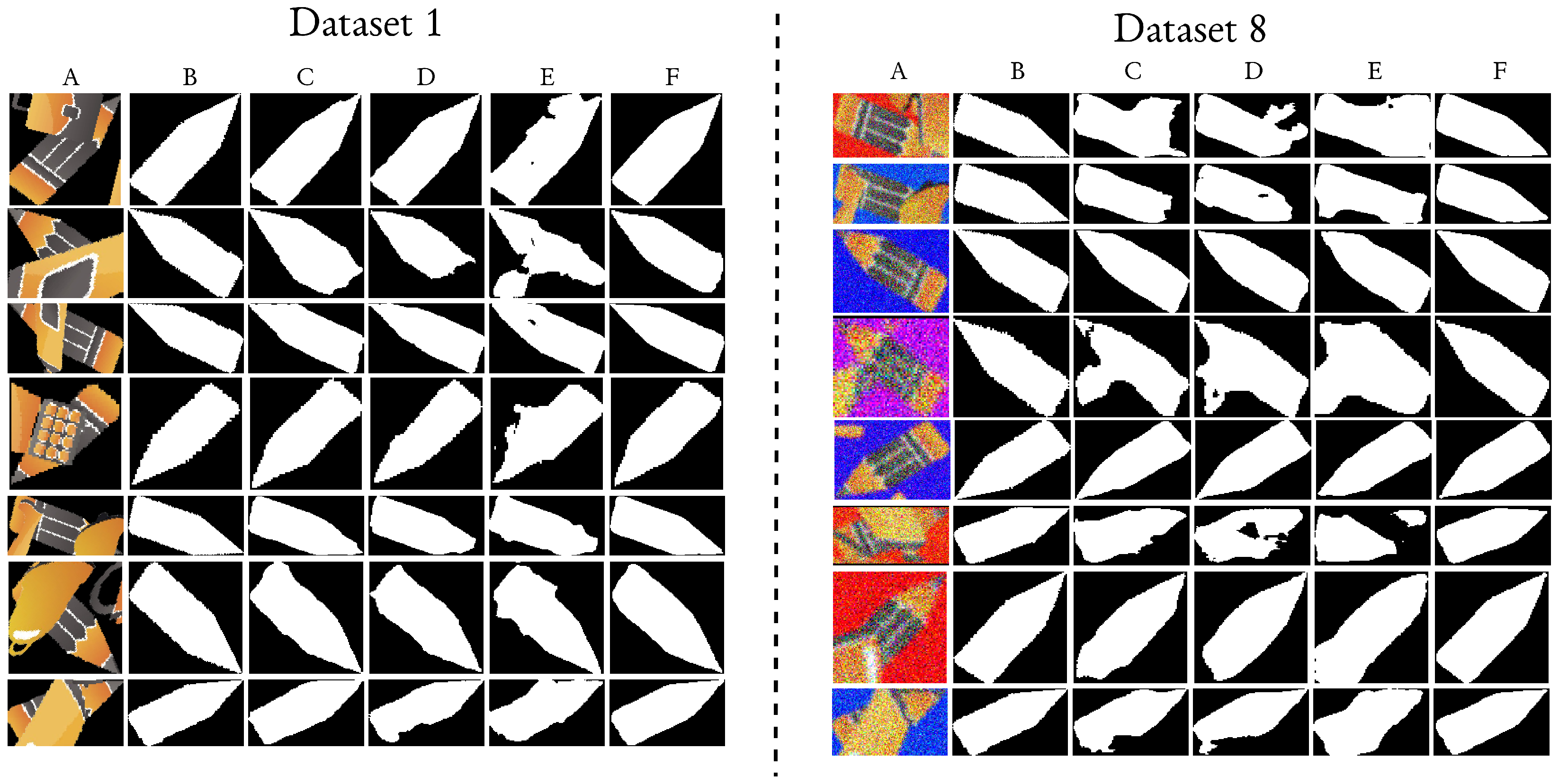
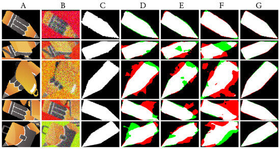
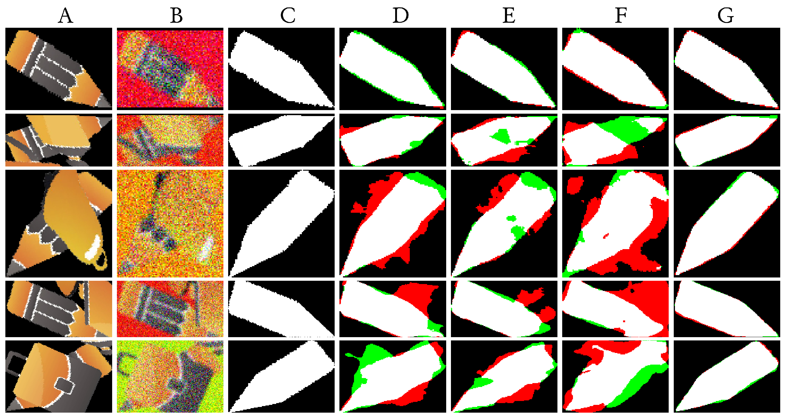
Sample prediction images are shown in Figure 8 and Figure 9. In Figure 9, to illustrate the models’ sensitivity to noise, prediction images corresponding to the input images of Dataset 1 and Dataset 8 are combined. The predictions for Dataset 1 are obtained from the merging of green and white regions, whereas those for Dataset 8 are derived from the merging of red and white regions. As observed in the selected examples, the proposed model successfully predicts the pencil object in both datasets, even under challenging conditions such as occlusion, noise, and blur.

Figure 8. Qualitative comparison of model predictions on Dataset 1 and Dataset 8. The (left panel) corresponds to Dataset 1, and the (right panel) corresponds to Dataset 8. (A) Input image, (B) ground-truth mask, (C) prediction by Attention U-Net, (D) prediction by U-Net, (E) prediction by FourierNet, and (F) prediction by FUNet.

Figure 9. Qualitative comparison of segmentation performance under noise/corruption. (A) Input image from Dataset 1. (B) Input image from Dataset 8. (C) Ground-truth mask. (D) Prediction by Attention U-Net. (E) Prediction by U-Net. (F) Prediction by FourierNet. (G) Prediction by FUNet.

To assess robustness against stochastic effects, the experiments were repeated three times with different random seeds while keeping all hyperparameters fixed, and the results are reported as mean ± standard deviation (SD). The performance on Dataset 1 was IoU = $0.9199\pm 0.0030$ and Dice = $0.9568\pm 0.0013$, while on Dataset 8 it was IoU = $0.8796\pm 0.0032$ and Dice = $0.9307\pm 0.0016$.

To support the observed gaps on Dataset 8 beyond aggregate averages, paired per-image differences in Dice between FUNet and each comparison model (FourierNet, UNet, and Attention U-Net) were analyzed across the 150 test samples. For all three comparisons, the paired differences deviated from normality (Shapiro–Wilk p values ranging from $1.308\times {10}^{-15}$ to $1.892\times {10}^{-14}$; D’Agostino $K^2$p values ranging from $7.904\times {10}^{-24}$ to $8.546\times {10}^{-24}$); therefore, two-sided Wilcoxon signed-rank tests are reported. FUNet significantly outperforms FourierNet ($p=3.72\times {10}^{-19}$, rank-biserial $r=0.842$; $\Delta$Dice mean/median $=0.0825/0.0757$) and shows a smaller but still significant advantage over UNet ($p=1.09\times {10}^{-5}$, $r=0.414$; $\Delta$Dice mean/median $=0.0111/0.0124$). FUNet also significantly outperforms Attention U-Net (Wilcoxon $W=3367$, $p=1.656\times {10}^{-5}$, rank-biserial $r=0.405$; $\Delta$Dice mean/median $=0.0097/0.0113$, $\mathrm{SD}=0.0727$), with a per-image win rate of $66.0\%$ ($\Delta >0$). These paired analyses confirm that the observed gains are not driven by aggregate averaging alone.

6. Discussion

In this study, frequency-domain-based deep learning methods were proposed as a solution to the image segmentation problem, and comparisons were made with existing spatial-domain models. The quantitative and qualitative results show that UNet-based encoder–decoder variants operating on low-frequency spectra provide the most reliable performance, particularly on the challenging Dataset 8. The paired statistical analyses on Dataset 8 further support that the proposed FUNet model provides a large and consistent improvement over FourierNet across test samples, while the improvements over UNet and Attention U-Net are smaller in magnitude but remain statistically significant.

A key observation is that the proposed formulation emphasizes global shape cues through low- and mid-frequency components. In the synthetic benchmark, blur and noise primarily corrupt fine-scale details, and heavy occlusion reduces the amount of local spatial evidence; however, the coarse geometry of the target object remains partially preserved in the stable central frequency region. By learning a direct mapping from the input spectrum to the mask spectrum within a compact window, FUNet can exploit these stable components while avoiding reliance on fragile high-frequency details that are more sensitive to degradations. This behavior is reflected by the relatively small performance drop from Dataset 1 to Dataset 8 for FUNet compared to other model families.

More broadly, operating on spectral components provides a complementary perspective to pixel-space processing and can be less sensitive to certain spatial variations (e.g., shifts and mild geometric changes), which can be beneficial under degradations such as blur and noise. In addition, frequency-domain representations can offer a compact way to emphasize the most informative components for a given task, which is particularly useful in controlled settings such as the proposed synthetic benchmark.

The FUNet-Thr and FUNet-BBox variants highlight the importance of how frequency components are selected. Magnitude-thresholding can discard informative coefficients when corruption alters magnitudes, and may introduce instability when the retained set varies across samples. Similarly, enlarging the effective window (as in FUNet-BBox) can include higher-frequency components that are less reliable under blur/noise, which can reduce overlap-based metrics on Dataset 8. Overall, these results suggest that a compact low-frequency core provides a robust representation for the target shape in the presence of challenging corruptions.

The observed degradation of the LSTM-based models is largely attributable to the mismatch between recurrent inductive bias and the structure of FFT features. FFT coefficients do not have a natural temporal order; thus, the chosen serialization strategy can strongly affect recurrent models. In LSTM-Patch, flattening the $w\times w$ frequency patch into a row-major sequence imposes an arbitrary ordering that does not necessarily preserve meaningful neighborhood relations in the frequency plane. In LSTM-Sorted, sorting tokens by magnitude produces a sample-dependent permutation, where the same sequence index may correspond to different $(u,v)$ locations across images, weakening consistent “adjacent token” dependencies. Moreover, FFT coefficients can exhibit a wide dynamic range; without appropriate normalization of the real/imaginary parts (and magnitude when used as input), recurrent units may saturate and optimization may become unstable.

As limitations of this study, the experiments are conducted on a single-target, single-class synthetic benchmark, which enables controlled evaluation under occlusion, noise, and blur, but still requires validation on real-world datasets and extension to multi-class and multi-instance settings. In addition, the current synthetic corruption model includes Gaussian noise and Gaussian blur, but does not cover impulse noise (salt-and-pepper) or non-uniform illumination. Future work will expand the corruption model with more realistic degradations, including spatially varying illumination (e.g., gradients, vignetting, and shadow-like bias), and will report robustness results after repeating training and hyperparameter selection under these expanded conditions. In addition, future studies may compare Fourier-based representations with alternative spectral decompositions, such as wavelet transforms, to better understand their relative robustness and suitability under different corruption types. Finally, frequency-domain representations can be combined with stronger attention-based backbones (e.g., Transformer encoders) to better capture long-range dependencies and to reduce sensitivity to token ordering [34].

7. Conclusions

This work proposed a frequency-domain instance segmentation framework that predicts the FFT coefficients of the target mask and reconstructs the binary mask via inverse FFT. Experiments on a controlled synthetic benchmark with occlusion, blur, and noise show that the proposed FUNet model achieves the best Dice/IoU on both the clean (Dataset 1) and corrupted (Dataset 8) settings, and significantly outperforms FourierNet on the challenging Dataset 8. Overall, the results indicate that focusing on stable low-frequency components can improve robustness under severe degradations. Future work will extend the evaluation to real-world datasets and to multi-class/multi-instance scenarios, and explore attention-based backbones for frequency-token representations.

References

- Zhang, D.; Lu, G. Shape-based image retrieval using generic Fourier descriptor. Signal Process. Image Commun. 2002, 17, 825–848. [Google Scholar] [CrossRef] [Scilit]
- Gonzalez, R.; Woods, R. Digital Image Processing; Addison-Wesley World Student Series; Addison-Wesley: Boston, MA, USA, 1992. [Google Scholar]
- Pal, N.R.; Pal, S.K. A review on image segmentation techniques. Pattern Recognit. 1993, 26, 1277–1294. [Google Scholar] [CrossRef] [Scilit]
- Bali, A.; Singh, S.N. A Review on the Strategies and Techniques of Image Segmentation. In 2015 Fifth International Conference on Advanced Computing & Communication Technologies; IEEE: New York, NY, USA, 2015; pp. 113–120. [Google Scholar]
- Bolya, D.; Zhou, C.; Xiao, F.; Lee, Y.J. Yolact: Real-time instance segmentation. In IEEE/CVF International Conference on Computer Vision; IEEE: New York, NY, USA, 2019; pp. 9157–9166. [Google Scholar]
- Minaee, S.; Boykov, Y.; Porikli, F.; Plaza, A.; Kehtarnavaz, N.; Terzopoulos, D. Image Segmentation Using Deep Learning: A Survey. IEEE Trans. Pattern Anal. Mach. Intell. 2022, 44, 3523–3542. [Google Scholar] [CrossRef] [Scilit] [PubMed]
- Riaz, H.U.M.; Benbarka, N.; Zell, A. FourierNet: Compact Mask Representation for Instance Segmentation Using Differentiable Shape Decoders. In 2020 25th International Conference on Pattern Recognition (ICPR); IEEE: New York, NY, USA, 2021; pp. 7833–7840. [Google Scholar]
- Lee, Y.; Park, J. Centermask: Real-time anchor-free instance segmentation. In IEEE/CVF Conference on Computer Vision and Pattern Recognition; IEEE: New York, NY, USA, 2020; pp. 13906–13915. [Google Scholar]
- Liu, S.; Qi, L.; Qin, H.; Shi, J.; Jia, J. Path aggregation network for instance segmentation. In IEEE Conference on Computer Vision and Pattern Recognition; IEEE: New York, NY, USA, 2018; pp. 8759–8768. [Google Scholar]
- Varghese, R.; Sambath, M. A Comprehensive Review On Two-Stage Object Detection Algorithms. In 2023 International Conference on Quantum Technologies, Communications, Computing, Hardware and Embedded Systems Security (iQ-CCHESS); IEEE: New York, NY, USA, 2023; pp. 1–7. [Google Scholar]
- He, K.; Gkioxari, G.; Dollár, P.; Girshick, R. Mask r-cnn. In IEEE International Conference on Computer Vision; IEEE: New York, NY, USA, 2017; pp. 2961–2969. [Google Scholar]
- Yu, Y.; Wang, C.; Fu, Q.; Kou, R.; Huang, F.; Yang, B.; Yang, T.; Gao, M. Techniques and Challenges of Image Segmentation: A Review. Electronics 2023, 12, 1199. [Google Scholar] [CrossRef] [Scilit]
- Hou, Y.; Guo, B.l.; Pan, J.S. The Application and Study of Graph Cut in Motion Segmentation. In 2009 Fifth International Conference on Information Assurance and Security; IEEE: New York, NY, USA, 2009; Volume 1, pp. 265–268. [Google Scholar]
- Rao, A.N.; Kumar, V.V.; Nagaraju, C. A New Segmentation Method using Watersheds on Grey Level Images. In 2006 International Conference on Advanced Computing and Communications; IEEE: New York, NY, USA, 2006; pp. 275–278. [Google Scholar]
- Ronneberger, O.; Fischer, P.; Brox, T. U-Net: Convolutional Networks for Biomedical Image Segmentation. In Medical Image Computing and Computer-Assisted Intervention—MICCAI 2015; Navab, N., Hornegger, J., Wells, W.M., Frangi, A.F., Eds.; Springer: Cham, Switzerland, 2015; pp. 234–241. [Google Scholar]
- Weber, M.; Wang, H.; Qiao, S.; Xie, J.; Collins, M.D.; Zhu, Y.; Yuan, L.; Kim, D.; Yu, Q.; Cremers, D.; et al. Deeplab2: A tensorflow library for deep labeling. arXiv 2021, arXiv:2106.09748. [Google Scholar]
- Jenkin, R. Digital image processing in the frequency domain. In The Manual of Photography; Routledge: Oxfordshire, UK, 2012; pp. 521–534. [Google Scholar]
- Beauchemin, S.S.; Barron, J.L. The frequency structure of one-dimensional occluding image signals. IEEE Trans. Pattern Anal. Mach. Intell. 2000, 22, 200–206. [Google Scholar] [CrossRef] [Scilit]
- Yilmaz, A.; Javed, O.; Shah, M. Object tracking: A survey. ACM Comput. Surv. (CSUR) 2006, 38, 13. [Google Scholar] [CrossRef] [Scilit]
- Cansiz, S.; Kesim, C.; Bektas, S.N.; Kulali, Z.; Hasanreisoglu, M.; Gunduz-Demir, C. FourierNet: Shape-Preserving Network for Henle’s Fiber Layer Segmentation in Optical Coherence Tomography Images. IEEE J. Biomed. Health Inform. 2023, 27, 1036–1047. [Google Scholar] [CrossRef] [Scilit] [PubMed]
- Jeon, Y.S.; Yang, H.; Feng, M. FCSN: Global Context Aware Segmentation by Learning the Fourier Coefficients of Objects in Medical Images. IEEE J. Biomed. Health Inform. 2024, 28, 1195–1206. [Google Scholar] [CrossRef] [Scilit] [PubMed]
- Khan, U.S.; Zhang, X.; Su, Y. Active Contour Model Using Fast Fourier Transformation for Salient Object Detection. Electronics 2021, 10, 192. [Google Scholar] [CrossRef] [Scilit]
- Liu, H.; Wang, C.; Zhao, J.; Chen, S.; Kong, H. Adaptive Fourier Convolution Network for Road Segmentation in Remote Sensing Images. IEEE Trans. Geosci. Remote Sens. 2024, 62, 5617214. [Google Scholar] [CrossRef] [Scilit]
- Xu, K.; Qin, M.; Sun, F.; Wang, Y.; Chen, Y.K.; Ren, F. Learning in the Frequency Domain. In 2020 IEEE/CVF Conference on Computer Vision and Pattern Recognition (CVPR); IEEE: New York, NY, USA, 2020; pp. 1737–1746. [Google Scholar]
- Pham, V.T.; Ha, M.H.; Bui, B.V.Q.; Hy, T.S. FFTMed: Leveraging Fast-Fourier Transform for a Lightweight and Adversarial-Resilient Medical Image Segmentation Framework. Sci. Rep. 2025, 15, 37879. [Google Scholar] [CrossRef] [Scilit] [PubMed]
- Erden, M.B.; Cansiz, S.; Caki, O.; Khattak, H.; Etiz, D.; Yakar, M.C.; Duruer, K.; Barut, B.; Gunduz-Demir, C. FourierLoss: Shape-aware loss function with Fourier descriptors. Neurocomputing 2025, 638, 130155. [Google Scholar] [CrossRef] [Scilit]
- Le, M.Q.; Tran, M.T.; Le, T.N.; Nguyen, T.V.; Do, T.T. CamoFA: A Learnable Fourier-Based Augmentation for Camouflage Segmentation. In 2025 IEEE Winter Conference on Applications of Computer Vision, WACV 2025; Qiu, Q., Setlur, S., Eds.; IEEE: New York, NY, USA, 2025; pp. 3427–3436. [Google Scholar]
- Ling, P.; Xiong, W. FrGNet: A fourier-guided weakly-supervised framework for nuclear instance segmentation. arXiv 2025, arXiv:2502.09874. [Google Scholar]
- Xing, R. FreqU-FNet: Frequency-Aware U-Net for Imbalanced Medical Image Segmentation. arXiv 2025, arXiv:2505.17544. [Google Scholar]
- Lv, C.; Lv, X.-L.; Wang, Z.; Zhao, T.; Tian, W.; Zhou, Q.; Zeng, L.; Wan, M.; Liu, C. A focal quotient gradient system method for deep neural network training. Appl. Soft Comput. 2025, 184, 113704. [Google Scholar] [CrossRef] [Scilit]
- Ting, K.M. Precision and Recall. In Encyclopedia of Machine Learning; Sammut, C., Webb, G.I., Eds.; Springer: Boston, MA, USA, 2010; p. 781. [Google Scholar]
- Zou, K.H.; Warfield, S.K.; Bharatha, A.; Tempany, C.M.; Kaus, M.R.; Haker, S.J.; Wells, W.M.; Jolesz, F.A.; Kikinis, R. Statistical validation of image segmentation quality based on a spatial overlap index1: Scientific reports. Acad. Radiol. 2004, 11, 178–189. [Google Scholar] [CrossRef] [Scilit] [PubMed]
- Jaccard, P. The Distribution Of The Flora in The Alpine Zone. New Phytol. 1912, 11, 37–50. [Google Scholar] [CrossRef] [Scilit]
- Shen, Q.; Zhang, J. MFTFormer: Meteorological-Frequency-Temporal Transformer with Block-Aligned Fusion for Traffic Flow Prediction. Res. Sq. 2026. preprint. [Google Scholar] [CrossRef] [Scilit]
Disclaimer/Publisher’s Note: The statements, opinions and data contained in all publications are solely those of the individual author(s) and contributor(s) and not of MDPI and/or the editor(s). MDPI and/or the editor(s) disclaim responsibility for any injury to people or property resulting from any ideas, methods, instructions or products referred to in the content. |
© 2026 by the authors. Licensee MDPI, Basel, Switzerland. This article is an open access article distributed under the terms and conditions of the Creative Commons Attribution (CC BY) license.