


Abstract
This paper addresses the challenge of estimating language minority populations for compliance with the U.S. Voting Rights Act (VRA). Current methodologies, which rely on frequentist and Bayesian models developed by the U.S. Census Bureau, are benchmarked against a novel machine learning approach. We use a random forest (RF) model that significantly improves population size estimates for language minority groups. Our key contribution is the development of a modified RF objective function, a beta–binomial distribution, which is specifically tailored to the unique structure of the VRA data. This approach leverages the flexibility of the RF framework to accommodate the VRA data in a statistically principled manner. The resulting RF method demonstrates superior performance on several language minority groups compared to the established 2021 Census Bureau models.
MSC:
62A99
1. Introduction
1.1. A Motivating Example
Section 203(b) of the Voting Rights Act (VRA) mandates that certain U.S. states and their political subdivisions (such as counties and townships) provide election materials in languages other than English. The U.S. Census Bureau determines which jurisdictions are subject to these requirements. This determination is based on the population counts and the proportions of limited English proficiency (LEP) and illiteracy within specific population subgroups, referred to as language minority groups (LMGs). For VRA compliance, the Census Bureau is required to estimate the weighted number of voting-aged (18 or older) individuals (VOT), voting-aged citizens (CIT), voting-aged citizens with limited English proficiency (LEP), and voting-aged citizens with limited English proficiency who are illiterate (ILL) within each relevant geographic area.
For jurisdiction i, let be the proportion of voting-aged persons who are citizens (CIT/VOT), be the proportion of voting-aged persons who are citizens with Limited English proficiency (LEP/VOT), and be the proportion of voting-aged persons who are illiterate citizens (ILL/VOT). CIT is estimated as the product of the direct (survey-weighted) estimate of VOT in jurisdiction i and an estimate of . A similar approach is used to estimate LEP and ILL. However, because the direct estimates of and are often zero for smaller areas, we model these proportions using Small Area Estimation (SAE) methods [1,2,3].
1.2. Previous Model for the 2021 Determinations
In 2021, the SAE modeled estimates of , , and were derived from the “multinomial logit normal” model [3]. We summarize this model for the CIT case below, noting that the models for LEP conditional on CIT and ILL conditional on LEP are similar. Let and be the VOT and CIT counts for some language minority group in jurisdiction i, respectively. is modeled as a draw from a binomial distribution with success probability and independent trials. The following logistic link function associates the feature vector with the outcomes of and :
For county i, this results in the following probability model for :
where is a Gaussian probability density function, with a random effects variable that is typical to small area estimation. The model is fit using the in-sample values for counts, and estimates as the product of these counts and the ratio of the survey-weighted estimates of and .
This parametric model was used in the 2021 VRA determinations [3] and had to make two critical assumptions: (1) an intrinsically linear relationship between the covariates and the values (i.e., is a linear combination of the ) and (2) no interactions among the features. In addition, features for the statistical models were selected prior to fitting based on a manual variable selection procedure. Any departure from these assumptions and/or incorrect variable selection can result in biased estimates of . One way to address this problem is to adopt machine learning (ML) methods. In this paper, we adopt a random forest model to improve the estimation of for the VRA determinations.
2. Random Forest Model for the VRA Determination
2.1. Understanding the Random Forest Method
This section briefly reviews the random forest method, emphasizing the role of an objective function used to split data when growing decision trees. In classical random forests, measures the discrepancy between observations and their average (e.g., mean squared error). Let denote the value of for the full dataset. When the data are partitioned into two complementary subsets, and represent the corresponding values on each subset, and each tree seeks splits that optimize . When is the mean squared error, this optimization involves minimizing ; however, in our application, is a probability function, and optimal splits are obtained by maximizing to identify the subgroup division with the highest probability. This process systematically searches over features and cut-off points to produce the most effective partition, after which the resulting subgroups are treated as homogeneous, and no additional features are required to compute , reflecting a fundamental principle of tree-based methods.
To explain this further, consider an outcome vector , for example, in our application, regressed on a feature matrix X. To associate these variables, we can fit a single regression tree model for . Let denote a constant probability value for county for , at a subgroup s that is a final node of a single tree. Then, the following equation can be considered:
where does not depend on X and can be used as a metric to grow a tree. Previous research efforts have grown trees with this concept [4,5,6].
In contrast to classical statistical approaches, which use the mean squared error for regression, we utilized a beta–binomial posterior probability as the objective function to build our trees, as explained in the next section. At each step of the random forest tree-building procedure, the algorithm selects one feature variable in combination with one split point that maximizes the probability function, with the parameter estimates directly derived from the tree nodes. This approach is computationally efficient, as the optimization of the probability function does not require an iterative procedure but is simply based on the estimates of the mean and the variance in the nodes. The idea of using the probability as a splitting criterion for growing a tree has been used in the context of the beta distribution [7] and other maximum likelihood functions [8].
Specifically in our application, we used the beta distribution to form the random forest trees. Namely, for county i, B random forest trees produce estimates of , , …, , where indicates that county i is in subgroup s of the random forest tree. The resulting ensemble estimate is simply .
2.2. Small Area Estimation with a Single Tree
In this section, we introduce a probability model that estimates , the model-based estimate of CIT/VOT for county i, in the context of the small area estimation [9]. When the number of voting-aged persons in a county is small, e.g., less than 1000, the direct estimate of this proportion is unreliable. Small area estimation assumes that the unobserved true proportions may have generated . Because our target parameter is rather than , we seek to model the posterior distribution of for county i:
which contains all the necessary information about . Recall that is just the ratio of to . Consider for a moment without considering . Then, for county i in subgroup s of a tree, Equation (1) can be expressed as a beta–binomial distribution, which results from combining a binomial likelihood with a beta prior distribution:
where is a constant parameter for all counties within subgroup S, i.e., for any two counties . Similarly, let and so that these sums are constant for any counties in S. denotes the probability density function of the beta prior distribution with shape parameters a and b for . Specifically, this function is , where . The hyperparameters a and b were chosen to be a small number () to ensure that the influence of the data dominates in the splitting procedure.
Due to the conjugacy of the beta–binomial distribution, the conditional posterior is
This posterior distribution can be extended for other outcome categories by replacing by or . The beta distribution has been applied successfully as an objective function to grow random forest trees in a different context [7]. Note that the random effects in this beta–binomial model are incorporated through the beta prior on .
2.3. The Tree Method for Estimating Parameters
Recall that all counties i within the subgroup S share the same constant probability , and that these counties are homogeneous with respect to X. In a single tree subgroup s, the following equality holds:
The data are to be split based on , which is . and are the total and counts for the subgroup S. Define as the data point that maximizes the following objective function:
where denotes a subgroup, for example, in Section 2.1, where a splitting covariate is less than while denotes the other subgroup where the covariate is larger or equal to . denotes the posterior mean of , which is . Thus, denotes the following:
which is calculated within the subgroup S. The following Algorithm 1 shows the algorithm for fitting a random forest tree method.
| Algorithm 1: Random forest algorithm for beta–binomial posterior |
|
The posterior mean of at a point is , where and are the total LEP and VOT counts for the subgroup S specified by of the random forest tree . The posterior means for were calculated in three models for , , and with the constraint that . There are 100 bootstrap samples for the jurisdictions and Alaskan Native Regional Corporations and 200 bootstrap samples for the American Indian areas. The tuning parameter values were from our empirical study that analyzed a large number of subpopulations, including 76 language minority groups across jurisdiction types and 51 within American Indian Areas/Alaska Native Regional Corporations, each with varying sample sizes.
2.4. Random Forest Issues with Unbalanced Data
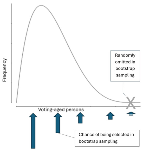
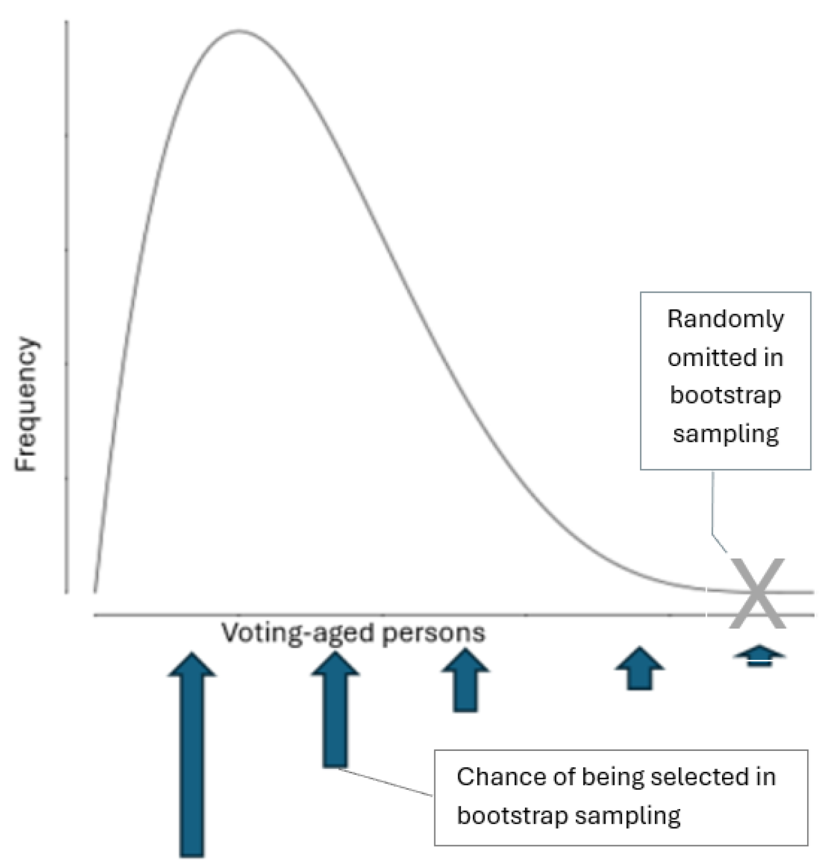
Figure 1 highlights the challenge of unbalanced data, specifically an extremely right-skewed distribution of voting-aged persons per jurisdiction for a generic language minority group. In this scenario, most jurisdictions have only one or two voting-aged persons, while the largest jurisdiction has 400. This disparity means that small jurisdictions have a significantly higher chance of being included in bootstrap resamples than larger jurisdictions.
Figure 1.
Hypothetical right-skewed distribution, with values on the horizontal axis and frequency on the vertical axis. The smallest arrow on the far right indicates the highest chance of omission in the classical bootstrap sample.
The over-representation of the smaller jurisdictions during sampling, indicated by the smallest arrow shown in Figure 1, leads to a substantial bias in random forest predictions for the larger jurisdictions, as the model will disproportionately learn from and be influenced by the characteristics of smaller jurisdictions.
3. Amplified Bootstrap Method
3.1. Colville Indian Language Minority Group Example
Table 1 presents a comparison of the values from an unbalanced dataset for the Colville Indian group with 112 jurisdictions, before and after the application of the amplified bootstrap method. The amplified bootstrap method extends the traditional bootstrap by allowing certain units in a dataset of n units to be ‘amplified’, meaning unit i appears an additional times, where is a non-negative integer. The metric indicates the difference between model-based estimates and estimates without a model (referred to as “direct estimates”), standardized by the standard error derived from these direct estimates [3]. This paper adopts the methodology of Slud et al. [2] to compare various models, utilizing the values across empirically determined sample size ranges.
Table 1.
Comparison of values before and after improvement.
Initially, in the “without amplification”, a notable imbalance was observed in the (200, 1 ] interval, where the value was . This significant value suggests a substantial discrepancy between the direct and modeled estimates in this range, driven by the insufficient representation of a large jurisdiction within that interval.
Following the application of the amplified bootstrap method, as shown in the “with amplification” row of Table 1, the values across all intervals demonstrate a remarkable change. The extreme value previously seen in the interval (200, 1 ] was significantly reduced, dropping from to . This drastic improvement indicates that the amplified bootstrap method effectively mitigated the bias caused by the unbalanced data, bringing the model-based estimates much closer to the direct estimates for this critical interval. The amplified bootstrap was also applied to the interval , resulting in an improvement of . The NA values for the interval indicate the absence of jurisdictions in the interval.
3.2. Basic Concept
Suppose, for example, jurisdiction i is the largest one. The following Table 2 sets to eight for jurisdiction i. Note that the first row represents the largest jurisdiction with 400 voting-aged persons. The third row shows copies after amplification. The last row displays each amplified sub-jurisdiction weighted with .
Table 2.
Arrows indicating amplification and weighting between row groups.
This process results in a total amplified sample size of . The core idea behind this amplification is to increase the representation of specific observations within the bootstrap sample, which can be particularly beneficial for highlighting rare or extreme data points.
In the standard bootstrap, the probability of selecting any given unit is . When considering the probability that a randomly selected unit from the amplified sample satisfies , we can express this as . Conventionally, this is approximated by . With amplification, the representation of each unit changes. After amplification, the probability of selecting any given unit (including its amplified copies) becomes , ensuring that all units within the amplified sample have an equal chance of being selected.
To maintain unbiased estimation, the contribution of each unit must be adjusted to account for its amplification with a modified weight for each i in the optimization procedure. This weighting scheme ensures that, despite being present multiple times, the overall influence of an amplified observation is appropriately normalized, preserving the statistical properties of the original sample.
3.3. Mathematical Understanding
The probability of a randomly selected unit being less than a certain value a can be expressed as its expected value, , where is the indicator function. This probability can be approximated by a summation over the sample, as shown in the sequence of equations below:
Equation (4) represents the standard bootstrap method. In this approach, each unit, which could represent a jurisdiction, is assigned a bootstrap weight of , meaning each unit has an equal probability of being selected from the original sample of size n.
Moving to Equation (5), this step introduces an amplification factor, denoted by . This factor allows for unit i to be amplified or replicated times in the resampled dataset. The term effectively shows how the equal weight is maintained conceptually before considering the total amplified size.
Equation (6) further elaborates on the amplification by incorporating the amplified sample size, . By multiplying and dividing by , this equation sets the stage to explicitly show the role of the amplified sample size in the probability calculation.
Finally, Equation (7) provides a comprehensive understanding of the amplified bootstrap. This equation reveals that after amplification, each unit i is effectively amplified times. When resampling from this amplified dataset, each of these instances of unit i has a chance of of being selected. Consequently, each unit i is assigned a weight of . This weighting ensures that the original proportional contribution of each unit is preserved, even though some units appear more frequently in the amplified sample.
Since remains the same throughout the entire splitting process, each unit i is assigned a weight of . With this weight, the counts in Equations (2) and (3) will be weighted as = instead of . This weighting is also applied to the other counts, including , , and . This type of weighting procedure is generally used in a standard classification and regression tree [10].
The mathematical derivation in Equations (4)–(7) demonstrates the theoretical equivalence between the classical and amplified bootstrap methods. Consequently, the bootstrap procedure is expected to yield equivalent results regardless of whether amplification is employed. Nevertheless, the omission of even a single critical data point in the classical sample can produce misleading estimates in finite bootstrap samples. As evidenced by the simulation study and real-world data in Section 3.1, this issue can be effectively attenuated through the amplification procedure.
3.4. Algorithm to Choose the Amplification Number
3.4.1. Example
The amplification number is determined based on the sample size intervals presented in a diagnostic table. To illustrate, recall Table 1, which contained an extreme value associated with the largest jurisdiction.
As highlighted in Table 3, a value of 10.59 is observed in the (200, 1 ] interval. This indicates an extreme deviation of the model-based estimate from the design-based estimate within this interval, primarily attributed to the largest jurisdiction of about 400 voting-aged persons. To improve this deviation, the largest jurisdiction is conceptually divided into eight smaller sub-jurisdictions, each comprising 50 voting-aged persons.
Table 3.
values before improvement.
The algorithm then sets the number 50 as a key value, which corresponds to the upper bound of the second-largest window of the diagnostic table, specifically the interval. Because the amplification number must be an integer, it is calculated as the integer part of , resulting in . This indicates that the original large jurisdiction is effectively amplified by a factor of eight to balance the data. Consequently, for each of these eight conceptual sub-jurisdictions, we assign 50 voting-aged persons, ensuring a more distributed representation within the dataset.
3.4.2. Generalized Algorithm
The process of determining the amplification number for given units, such as a jurisdiction, is based on identifying extreme deviations observed in a diagnostic table. This table categorizes units by their sample size intervals and reports diagnostic metrics, such as , which quantifies the bias or imbalance within each interval.
Let be the set of M (=6) predefined sample size intervals in the diagnostic table, where each interval has a lower bound and an upper bound . For each interval , a diagnostic metric value, , is observed.
The algorithm proceeds as follows:
- Identify Extreme Interval: Locate the interval for which the diagnostic metric exhibits an extreme value. This extreme value typically signifies a significant imbalance or bias concentrated within units falling into this sample size range. For instance, if represents , an extremely high positive value might indicate substantial bias for units in this interval.
- Identify Influential Unit: Within the identified extreme interval , pinpoint the specific unit i (e.g., a jurisdiction) that is primarily responsible for the observed extreme value. Let denote the number of persons (or sample size) associated with this influential unit i.
- Determine Target Sub-Unit Size: Select a target sample size, , for the conceptual sub-units. This is typically chosen to align with an upper bound of a “well-behaved” or less extreme interval in the diagnostic table. This is an interval that represents a more desirable distribution of sample sizes, such as the upper bound of the second-largest window, , where for k is typically (=6).
- Calculate Amplification Number : The amplification number for the influential unit i is calculated as the integer part of the ratio of its original sample size to the target sub-unit size:Since represents the number of additional times unit i will appear conceptually (or how many sub-units it will be divided into), it must be a non-negative integer.
- Distribute Unit’s Sample Size: Conceptually divide the influential unit i into sub-units. Each of these sub-units will then be assigned a sample size of (if is perfectly divisible by ), or more generally, the units are treated as if they were independent units, each contributing to the overall sample in a way that respects the new target size. If the division is not exact, the remainder might be handled by adjusting one of the sub-units or by distributing it across them. This process effectively redistributes the influence of the large unit across multiple, smaller conceptual units that fit better into more desirable intervals of the diagnostic table.This algorithm aims to ensure that an extreme diagnostic value caused by the largest jurisdiction is mitigated by conceptually dividing the jurisdiction and amplifying its representation to improve the prediction accuracy for the largest jurisdiction. Note that can be increased further because the weights adjust back, as explained in Section 3.3. The amplification is applied to all outcomes: VOT, CIT, LEP, and ILL.
4. Simulation Study
To evaluate the performance of our proposed method, a simulation study was conducted. The study was designed to mimic real-world conditions for our voting sample, using 100 random samples, each of size . The simulated data were generated with an imbalanced, right-skewed distribution, which frequently occurs in our voting data.
4.1. Data Generation Process
The voting population sizes for each jurisdiction were simulated as non-zero positive integers drawn from a Gamma distribution, specifically , with the addition of one to ensure all values are positive. The Gamma distribution was chosen for its ability to model skewed, non-negative data, which is characteristic of jurisdiction sizes, as shown in Figure 1. Specifically, we imposed two conditions. The largest value in each sample must fall within the interval , and all other values in the sample must be less than 200 so that the density of simulated data may possess a distribution highly skewed towards smaller values, with a long tail extending towards larger numbers.
The probability of an event (LEP/VOT) was simulated using a beta distribution, which is ideal for modeling probabilities, as its values are confined to the interval . Random values were generated for specific sample size intervals to serve diagnostic purposes. The beta parameters were chosen to align the mean probability of an event within each interval, as shown in Table 4.
Table 4.
and values for sample size intervals.
Three primary covariates were also generated for each of the six intervals, for : a normal distribution , a Poisson distribution , and a binomial distribution . These distributions were selected to represent different types of covariate data commonly found in statistical studies. These covariates were used to create nine decile dummy variables based on the Mahalanobis distance of the three variables. The Mahalanobis distance measures the distance between a point and a distribution, accounting for correlations between variables. This process introduced a set of independent variables that could influence the outcome, adding a layer of complexity and realism to the simulation.
4.2. Results
A key metric for evaluation was the standardized delta () value, a normalized measure of the difference between the true and estimated LEP counts. This metric provides a standardized way to compare model performance across different intervals and samples, with a lower value indicating a better model fit.
Table 5 shows the results for a single representative sample () with and without amplification.
Table 5.
Simulated data results with and without amplification.
The metrics used in the two tables above are defined as follows: #Juris refers to the number of jurisdictions in each sample size interval. , or standardized delta, is a measure of the difference between the true number of LEP individuals and the estimated number, divided by the variance of the true LEP count.
As shown in the tables, the value for the largest jurisdiction (in the interval) improved from 2.668 without amplification to 0.678 with amplification. This result is significant because the largest jurisdictions are often the most challenging to estimate due to their size and complexity.
Across all 100 simulated samples, amplification led to a reduction in the value for the largest jurisdiction in 97% of the samples. This high improvement rate indicates the robustness and reliability of the method. Three of the 100 random samples did not require or benefit from amplification, as their initial values were already low, at 0.049, 0.063, and 1.484, respectively.
5. Data Description and Analysis Results
5.1. Data Description
This paper uses five-year data from the American Community Survey (ACS) 2019–2023. ACS releases one- and five-year data products. The five-year products collected data over five years, allowing increased statistical precision of population estimates. The five-year data are particularly useful for estimating characteristics of small geographic areas or small domains in which one-year estimates are too imprecise for release under Census Bureau statistical quality guidelines. Some of the most important feature variables used to build covariates for each jurisdiction are as follows:
- Logit-transformed proportion of citizens among VOT persons
- Logit-transformed proportion of limited English-proficient among CIT
- Proportion of non-Hispanic White among VOT persons in a county
- Proportion of VOT persons with no college education in a county
- Average person count per housing unit among VOT persons in a county
- Average age among VOT persons in any AIAN LMG in a county
- Proportion of VOT persons in poverty in a county
- Proportion of speaking other languages at home among VOT persons in a county
- Proportion of foreign-born persons among VOT persons in a county
- Average years in the U.S. (as of 2019) among VOT foreign-born persons in a county.
The full list of covariates is included in Slud et al. [2].
5.2. Improvement Results by the Random Forest Method
This section presents the overall improvement of random forest with amplified bootstrap over the Bayesian multinomial random-effects model with random intercepts [11] for 2023 data, measured by , which quantifies the departure of model predictions from the actual data. The improvement is specifically highlighted for the cases where . The analysis is broken down by two types: jurisdictions and American Indian areas, with different ranges of observations presented in columns. “Imp%if>1.96” represents the percentage of random forest’s improvement rates among LMGs that have . “sum(>1.96)” indicates the number of LMGS that satisfy this condition.
5.2.1. Jurisdictions
Table 6 below summarizes random forest’s performance in jurisdictions across various sample size ranges:
Table 6.
Random forest’s performance across jurisdictions.
For jurisdictions with sample sizes in the ranges of (0, 4], (12, 25], and (25, 50], random forest demonstrated an improvement rate of 100% where . In the (4, 12] range, the improvement rate was 75.0%. In particular, there were no instances where for the (50, 200] and (200, 1 ] ranges, resulting in “NaN” for the improvement percentage and a count of zero. The highest number of LMGs that showed significant improvement was 10 in the (0, 4] observation range.
5.2.2. American Indian Areas
Table 7 details the improvement of random forest in American Indian areas:
Table 7.
Random forest’s improvement in American Indian areas.
In American Indian areas, random forest consistently showed a 100% improvement rate for observation ranges up to (50, 200]. For the largest observation range, (200, 1 ], the improvement rate was 50%. The number of LMGS with significant improvement ranged from one to two across these categories.
Random forest generally exhibits improvement over Bayes, particularly in smaller observation ranges for both jurisdictions and American Indian Areas. The absence of significant deviations in larger observation ranges for jurisdictions suggests that the models’ predictions might be more aligned with the data in those scenarios, or that the criteria for improvement are not met. In contrast, American Indian Areas show improvement across all presented observation ranges, albeit with a reduced rate in the highest range.
6. Variance Estimation for Random Forest Predictions via Successive Difference Replication
Let U denote a finite population of size N, and be the set of all possible samples under a complex design with selection probability for . For a realized sample s, equipped with design weights , let denote the fitted random forest parameters, defined by its ensemble of trees, node splits, and terminal predictions obtained via bootstrap resampling and feature subsampling of the weighted data. The prediction functional at covariate value x is
where maps a fitted forest to its prediction.
In a design-based framework, randomness in arises from the sampling design. In writing , the design-based variance is
where S is random under . Conceptually, can be regarded as a mixture of two effects: (i) sampling fluctuation, reflecting the difference between the model trained on the realized sample and the model that would have been trained on the full population, and (ii) parameter-estimation fluctuation, reflecting the randomness inherent in model fitting. Formally, let denote the population-fitted forest, i.e., the random forest one would obtain if the fitting procedure were applied to the entire finite population U. Then, we can idealize
where indicates the prediction using the replicate sample () with its fitted random forest parameter (), and indicates the prediction using the base full sample () with its fitted random forest parameter ().
Note that in practice, these two components are inseparable. This decomposition is useful only for intuition. Each replicate recomputes on a pseudo-sample, so replicate variation already reflects both sources jointly.
Successive Difference Replication (SDR) provides a design-consistent variance estimator for . Given replicate weight vectors , let denote the full-sample prediction and the prediction under replicate r. The replicate fluctuation is , and the SDR variance estimator is
where c is the SDR scaling constant (with in the standard construction, reflecting the successive-difference pairing). For our example, with replicates, .
Specifically, the SDR variance estimation process begins with the calculation of a point estimate, , which is the count of CIT, LEP, or ILL, by training a random forest model across the entire dataset using the full sample weights. This estimate is given by
where are the weighted counts of the entire sample for unit j, and is the predicted probability from the trained random forest, which is for CIT, LEP, or ILL.
The SDR method then repeats the entire modeling process for each of the sets of replicate weights. For each replicate, a new random forest model is trained. This new model is used to generate a replicate estimate, , for :
The key here is that both the replicate weights () and the model predictions () vary across replicates, ensuring that both sampling and model uncertainty are captured.
The final variance is calculated using the dispersion of the replicate estimates around the full-sample estimate. For the SDR method, the formula is as follows:
7. Discussion
This work applies the random forests (RF) method to refine the estimation of voting-aged persons within U.S. jurisdictions. A key challenge in the Small Area Estimation (SAE) framework is the absence of observed outcomes for validation. Unlike typical machine learning development, which relies on cross-validation to compare predicted and observed outcomes, the unique constraints of SAE, where even the simplest models like beta–binomial do not have observed outcomes, necessitated custom diagnostic measures, based on established research by Slud et al. [2] and Hall et al. [11].
Our RF method demonstrated significant improvements in prediction accuracy over the Bayesian multinomial random-effects model with random intercepts [11], which outperformed models for the 2021 determinations. The 2021 determination used various models ranging from the simplest beta–binomial model to multinomial random-effects models with random intercepts. A principal difference between our RF method and all others is that our RF uses the beta–binomial model as the objective function to split data and to build trees because the random forest model’s objective functions are typically simple, e.g., least squares or entropy-related measures.
A potential pitfall associated with RF, particularly when based on bootstrap resampling, is the risk of bias if jurisdiction units with extremely large sample sizes are not adequately represented or are inadvertently excluded from the bootstrap samples. To enhance the robustness of our predictions, we implemented the amplification bootstrap technique. This approach aims to mitigate bias by increasing the probability of including the largest jurisdictions within the bootstrap sample. The amplification bootstrap method is theoretically equivalent to the ordinary bootstrap method, ensuring that while it addresses specific bias concerns, it maintains the fundamental statistical properties of traditional bootstrapping.
Our model employs the classical random forest framework, which optimizes a beta–binomial posterior density using small hyperpriors. It is important to note that our approach does not specify a complete Bayesian posterior distribution for the entire model fitting process.
Estimating the variance of a prediction from our random forest model is consistent with a replication-based SDR approach, as outlined by Slud et al. [2]. Through the variability of replicate estimates, the SDR method implicitly captures the sampling variance attributable to the survey design (e.g., unequal probabilities of selection) as well as the model variance resulting from the random processes inherent in the model-building algorithm (e.g., bootstrapping and random feature selection in a random forest). The diagnostic measures and sample size ranges employed in this paper are sourced from Slud et al. [2], while that study focuses on point estimation, applying these methods to variance represents a promising direction for subsequent investigation.
Author Contributions
Conceptualization, J.K. and A.C.H.; Data curation, A.C.H.; Formal analysis, J.K. and A.C.H.; Methodology, J.K. and A.C.H.; Project administration, J.K.; Software, J.K., A.C.H., and G.L.; Supervision, J.K.; Validation, J.K.; Visualization, J.K. and A.C.H.; Writing—original draft preparation, J.K.; Writing—Review and Editing, A.C.H. All authors have read and agreed to the published version of the manuscript.
Funding
The research of Geunseop Lee was supported by the Hankuk University of Foreign Studies Research Fund.
Institutional Review Board Statement
Not applicable.
Informed Consent Statement
Not applicable.
Data Availability Statement
The datasets presented in this article are not readily available because they are protected by Title 13, U.S.C. in the interests of respondent privacy.
Conflicts of Interest
The authors declare no conflicts of interest.
References
- Joyce, P.M.; Malec, D.; Little, R.J.; Gilary, A.; Navarro, A.; Asiala, M.E. Statistical Modeling Methodology for the Voting Rights Act Section 203 Language Assistance Determinations. J. Am. Stat. Assoc. 2014, 109, 36–47. [Google Scholar] [CrossRef] [Scilit]
- Slud, E.V.; Ashmead, R.; Joyce, P.; Wright, T. Statistical Methodology (2016) for Voting Rights Act, Section 203 Determinations. 2018. Available online: https://www.census.gov/content/dam/Census/library/working-papers/2018/adrm/RRS2018-12.pdf (accessed on 20 February 2026).
- Slud, E.V.; Franco, C.; Hall, A.; Kang, J. Statistical Methodology (2021) for Voting Rights Act, Section 203 Determinations. 2022. Available online: https://www.census.gov/content/dam/Census/library/working-papers/2022/adrm/RRS2022-06.pdf (accessed on 20 February 2026).
- Kang, J.; Su, X.; Hitsman, B.; Liu, K.; Lloyd-Jones, D. Tree-structured analysis of treatment effects with large observational data. J. Appl. Stat. 2012, 39, 513–529. [Google Scholar] [CrossRef] [Scilit]
- Kang, J.; Su, X.; Liu, K. Tree-structured assessment of causal odds ratio with large observational study data sets. J. Data Sci. 2012, 10, 757–776. [Google Scholar] [CrossRef] [Scilit]
- Kang, J.; Su, X.; Liu, L.; Daviglus, M.L. Causal inference of interaction effects with inverse propensity weighting, G-computation and tree-based standardization. Stat. Anal. Data Min. ASA Data Sci. J. 2014, 7, 323–336. [Google Scholar] [CrossRef] [Scilit]
- Weinhold, L.; Schmid, M.; Mitchell, R.; Maloney, K.O.; Wright, M.N.; Berger, M. A Random Forest Approach for Bounded Outcome Variables. J. Comput. Graph. Stat. 2020, 29, 639–658. [Google Scholar] [CrossRef] [Scilit] [PubMed]
- Su, X.; Wang, M.; Fan, J. Maximum Likelihood Regression Trees. J. Comput. Graph. Stat. 2012, 13, 586–598. [Google Scholar] [CrossRef] [Scilit]
- Rao, J.N.K.; Molina, I. Small Area Estimation; John Wiley & Sons: Hoboken, NJ, USA, 2015. [Google Scholar] [CrossRef] [Scilit]
- Therneau, T.; Atkinson, B.; Ripley, B. rpart: Recursive Partitioning, R package version 4.1.24.; R Foundation for Statistical Computing: Vienna, Austria, 2025.
- Hall, A.C.; Kang, J. Inference with Pólya-Gamma Augmentation for US Election Law. Mathematics 2025, 13, 945. [Google Scholar] [CrossRef] [Scilit]

Disclaimer/Publisher’s Note: The statements, opinions and data contained in all publications are solely those of the individual author(s) and contributor(s) and not of MDPI and/or the editor(s). MDPI and/or the editor(s) disclaim responsibility for any injury to people or property resulting from any ideas, methods, instructions or products referred to in the content. |
© 2026 by the authors. Licensee MDPI, Basel, Switzerland. This article is an open access article distributed under the terms and conditions of the Creative Commons Attribution (CC BY) license.