Bivariate Generalized Split-BREAK Process with Application in Modeling Crime Dynamics

Abstract

The manuscript proposes a new non-linear and non-stationary bivariate stochastic model, termed the two-dimensional Gaussian (generalized) Split-BREAK (2D-GSB) process, as a multivariate extension of the univariate GSB framework. The generalization consists in introducing a common threshold mechanism based on the norm of a bivariate innovation vector and a single synchronized Bernoulli indicator which jointly governs regime activation in both components. This structure induces cross-dependent regime shifts and yields a binomial–Gaussian mixture representation of the joint distribution, explicitly linking contemporaneous dependence with a common latent regime mechanism. The fundamental properties of the proposed model are established, with particular emphasis on its asymptotic behavior. Parameter estimation procedure is developed using both the method of moments (MoM) and the empirical characteristic function (ECF) approach, and their performance is evaluated through Monte Carlo simulations. An empirical application to daily crime data illustrates how the proposed framework captures synchronized structural shocks and heavy-tailed features in related crime categories. In comparison with a standard VAR(1) benchmark, the 2D-GSB specification provides a parsimonious yet substantially improved likelihood-based fit, thus offering a theoretically sound framework for analyzing multivariate time series characterized by synchronized regime shifts and heavy-tailed behavior.

1. Introduction

The stochastic permanent break (STOPBREAK) process was first proposed by Engle and Smith [1] as a framework for modeling time series with permanent breaks and large fluctuations. Subsequently, many authors have considered models that rely, to a greater or lesser extent, on the concepts underlying the STOPBREAK process, primarily in the field of econometrics [2,3,4,5,6,7,8,9,10]. One generalization of this process, termed the Split-BREAK process, was proposed by Stojanović et al. [11] and Jovanović et al. [12]. Building on this framework, the Gaussian (or generalized) Split-BREAK (GSB) process is developed, extending the original model by introducing Gaussian innovations and latent dynamics with a Bernoulli noise indicator. Note that in the existing literature, the term “generalized” refers to the latent-mixture construction introduced in [11], which generalizes the basic STOPBREAK model introduced in [1]. Accordingly, in the present paper the innovation distribution is explicitly assumed to be Gaussian. In the aforementioned works, the distributive and asymptotic properties of the GSB process were established, along with various parameter estimation methods. In addition, the main distributional characteristics and empirical characteristic function (ECF)-based estimation procedures are discussed in detail in Stojanović et al. [13], while modifications involving Laplace and Cauchy innovations are presented in Stojanović et al. [14] and Ljajko et al. [15], respectively.

From a practical perspective, the GSB process has been applied to various empirical contexts, including stock market capitalization on the Belgrade Stock Exchange and the dynamics of infected and vaccinated individuals during the COVID-19 pandemic. These applications highlight the broader practical potential of the GSB model in economic and social dynamics. On the other hand, many real-world phenomena are manifested through several interrelated time series that evolve jointly. For instance, in a criminological context, time series representing ordinary robberies and aggravated robberies (organized or violent) are often correlated. In addition, common social factors (economic crisis, change in police strategies, or seasonal effects) may simultaneously generate spikes in both series, while each retains its own dynamics and internal structural properties.

While the univariate GSB model accounts for threshold-driven regime behavior within a single series, it cannot explicitly describe synchronized correlation structures across multiple time series. A key structural feature of the proposed 2D-GSB framework is the use of a single synchronized Bernoulli indicator $q_t\left(c\right)$, determined by the magnitude of the common innovation vector, whose formal definition is provided in Section 2. This structural modification represents the essential extension from the univariate GSB model and enables both components of the process to enter or exit a regime simultaneously, reflecting situations in which related time series (e.g., different but related crime types) are jointly affected by a common external shock (e.g., policy change, economic crisis). By linking regime activation directly to the innovation norm, the model captures coordinated abrupt changes in a transparent and analytically tractable manner, thereby extending the previous univariate GSB structure to the multivariate setting.

In particular, conventional VAR and multivariate GARCH frameworks may struggle to capture synchronized regime shifts driven by common shocks, since regime activation is not explicitly linked to innovation magnitudes. Instead of relying solely on linear dependence or volatility-based dynamics, typical of the aforementioned conventional multivariate specifications, the proposed 2D-GSB model includes a common threshold-driven regime indicator, determined by the magnitude of multivariate innovations. In this way, it allows for the capture of synchronized structural shocks and persistent regime effects within a single latent framework. More broadly, the proposed 2D-GSB framework is related to multivariate regime-switching and latent-state models, where structural changes are governed by unobserved mechanisms (for some recent ones, see, e.g., [16,17]). Unlike classical Markov-switching approaches, where regime transitions are driven by latent state dynamics, the regime activation in the 2D-GSB model is directly determined by the magnitude of innovations through a threshold mechanism. This places the proposed framework within the broader class of regime-dependent multivariate models while preserving analytical tractability through its binomial–Gaussian mixture representation.

In the following Section 2, the definition and basic stochastic structure of the 2D-GSB process are presented. Thereafter, Section 3 discusses additional stochastic properties of the 2D-GSB model, focusing on the distribution of its components and their asymptotic behavior. For this purpose, as in the one-dimensional GSB case, the characteristic function (CF) method is employed. Section 4 describes estimation procedures for the unknown parameters of the 2D-GSB process and establishes the asymptotic properties of the resulting estimators. In Section 5, Monte Carlo simulations of the proposed estimators are carried out, as well as an empirical application of the 2D-GSB process in the analysis of the dynamics of certain criminal offenses. Finally, Section 6 provides concluding remarks.

2. Definition and Structure of the 2D-GSB Process

As mentioned above, the two-dimensional generalized (or Gaussian) Split-BREAK (2D-GSB) process extends the univariate GSB framework by allowing two interrelated time series to evolve under regime-switching dynamics driven by large innovations. When the regime indicators are synchronized across both series, the resulting correlation structure and joint dynamics become particularly rich and suitable for modeling real-world systems characterized by parallel disturbances or transitions. The basic definitions of the 2D-GSB series can be given as follows.

Let ${\mathit{Y}}_{\mathit{t}}={(Y_t^{\left(1\right)},Y_t^{\left(2\right)})}^{\mathrm{\top }}$ be a bivariate time series defined on discrete time $t\in {\mathbb{N}}_0$. The process $\left({\mathit{Y}}_{\mathit{t}}\right)$ evolves according to the 2D-GSB structure if the following equality holds:

$${\mathit{Y}}_{\mathit{t}}=\left[\begin{array}{c}{Y}_t^{\left(1\right)}\\ Y_t^{\left(2\right)}\end{array}\right]={\mathit{\mu }}_{\mathit{t}}+{\mathit{\epsilon }}_{\mathit{t}}.$$

(1)

Here, ${\mathit{\epsilon }}_{\mathit{t}}={({\epsilon }_t^{\left(1\right)},{\epsilon }_t^{\left(2\right)})}^{\mathrm{\top }}~\mathcal{N}({\mathbf{0}}_{\mathbf{2}\times \mathbf{1}},\Sigma )$ are the independent identically distributed (IID) innovations with bivariate Gaussian distribution and the variance–covariance matrix

$$\Sigma =\left[\begin{array}{cc}{\sigma }_1^2& \rho {\sigma }_1{\sigma }_2\\ \rho {\sigma }_1{\sigma }_2& {\sigma }_2^2\end{array}\right],$$

where ${\sigma }_1,{\sigma }_2>0$ are the standard deviations of univariate series $\left({\epsilon }_{\mathrm{t}}^{\left(1\right)}\right),\left({\epsilon }_{\mathrm{t}}^{\left(2\right)}\right)$, respectively, and $\left|\rho \right|<1$ is their correlation. We also suppose that innovations $\left({\mathit{\epsilon }}_{\mathit{t}}\right)$ are defined based on the same probability space $\left(\Omega ,\mathcal{F},P\right)$, expanded by some filtration $F=\left({\mathcal{F}}_t\right).$ Thus, the conditional mean and variance of $\left({\mathit{\epsilon }}_{\mathit{t}}\right)$ are, respectively,

$$E\left({\mathit{\epsilon }}_{\mathit{t}}|{\mathcal{F}}_{t-1}\right)={\left(\mathrm{0,0}\right)}^{\mathrm{\top }}={\mathbf{0}}_{\mathbf{2}\times \mathbf{1}}, \mathrm{V}\mathrm{a}\mathrm{r}\left({\mathit{\epsilon }}_{\mathit{t}}|{\mathcal{F}}_{t-1}\right)=\mathbb{E}\left({\mathit{\epsilon }}_{\mathit{t}}^2|{\mathcal{F}}_{t-1}\right)=\Sigma .$$

(2)

Additionally, ${\mathit{\mu }}_{\mathit{t}}={({\mu }_t^{\left(1\right)},{\mu }_t^{\left(2\right)})}^{\mathrm{\top }}$ is a regime-sensitive latent mean vector process, termed the martingale mean process, defined by the recurrence relation:

$${\mu }_t^{\left(i\right)}={\mu }_{t-1}^{\left(i\right)}+q_{t-1}{\epsilon }_{t-1}^{\left(i\right)}={\mu }_0^{\left(i\right)}+\sum _{j=0}^{t-1}{q}_j{\epsilon }_j^{\left(i\right)}, i=\mathrm{1,2}.$$

(3)

Here, the equalities ${\mu }_0^{\left(i\right)}\stackrel{as}{=}{m}_i (const.)$, $i=\mathrm{1,2}$ hold almost surely (a.s.), while $\left(q_t\right)$ is the noise indicator, i.e., the Bernoulli process defined by the equalities

$$q_t(\mathrm{c})=I\left\{{‖{\mathit{\epsilon }}_{\mathit{t}-\mathbf{1}}‖}^2>c\right\}=\left\{\begin{array}{c}1, {\left({\epsilon }_{t-1}^{\left(1\right)}\right)}^2+{\left({\epsilon }_{t-1}^{\left(2\right)}\right)}^2>c\\ 0, {\left({\epsilon }_{t-1}^{\left(1\right)}\right)}^2+{\left({\epsilon }_{t-1}^{\left(2\right)}\right)}^2\le c\end{array}\right., t=\mathrm{1,2},\dots$$

(4)

where $‖·‖$ is the usual Euclidean norm in ${\mathbb{R}}^2$ and $q_0\left(c\right)\equiv 1$. The value $c>0$ represents the critical value of reaction, i.e., the magnitude of past innovations $\left({\mathit{\epsilon }}_{\mathbf{t}}\right)$ determines whether the current innovation is incorporated into the latent process (${\mathit{\mu }}_{\mathit{t}}),$ as defined in Equation (3). More precisely, when $q_{t-1}=0$, there is no change in the martingale means ${\mu }_t^{\left(i\right)}, i=\mathrm{1,2},$ relative to their previous values ${\mu }_{t-1}^{\left(i\right)}$, implying that $Y_t^{\left(i\right)}$ exhibits only a “small” fluctuation driven solely by ${\epsilon }_t^{\left(i\right)}$. Conversely, when $q_{t-1}=1,$ the process undergoes a pronounced (permanent) shift, resulting in a more substantial fluctuation of $Y_t^{\left(i\right)}$.

Thus, the regime switch in the 2D-GSB process is driven by an innovation threshold; that is, realized values of $\left({\mathit{\epsilon }}_{\mathit{t}}\right)$ determine the intensity of fluctuations in the underlying series $\left({\mathit{Y}}_{\mathbf{t}}\right)$. Moreover, the synchronized indicator $q_t\left(c\right)$, defined in Equation (4), enables joint regime detection across both components of $\left({\mathit{\epsilon }}_{\mathit{t}}\right)$, capturing structurally linked shocks in correlated innovation processes $\left({\epsilon }_t^{\left(i\right)}\right), i=\mathrm{1,2}$. This feature is particularly important when modeling interdependent time series, such as different but related categories of crime, which are discussed below. It also facilitates a coherent interpretation of latent dynamics and common external shocks.

Now, similar to the one-dimensional case (see, e.g., Jovanović et al. [12]), the following properties of the above-mentioned time series can be proven.

Theorem 1.

Let $\left({\mathit{\mu }}_{\mathit{t}}\right)$ and $\left({\mathit{Y}}_{\mathit{t}}\right)$ be the two-dimensional stochastic processes defined by Equations (1)–(4). Then, both of these series have a constant and equal mean values

$$\mathbb{E}\left({\mathit{\mu }}_{\mathit{t}}\right)=\mathbb{E}\left({\mathit{Y}}_{\mathit{t}}\right)={\left(m_1,m_2\right)}^{\top },$$

while their covariance matrices are, respectively,

$${\Gamma }_{\mu }\left(s,t\right)=Cov \left({\mathit{\mu }}_{\mathit{s}},{\mathit{\mu }}_{\mathit{t}}\right)=\left\{\begin{array}{cc}{p}_c·t·\Sigma ,& s=t\\ p_c·\mathit{min}\left(s,t\right)·\Sigma ,& s\ne t\end{array}\right.,$$

(5)

$${\Gamma }_Y\left(s,t\right)=Cov \left({\mathit{Y}}_{\mathit{s}},{\mathit{Y}}_{\mathit{t}}\right)=\left\{\begin{array}{cc}\left(1+p_{c}t\right)·\Sigma ,& s=t\\ p_c·\left(1+\mathit{min}\left(s,t\right)\right)·\Sigma ,& s\ne t.\end{array}\right.$$

(6)

where $p_c=E\left(q_t\right)=P\left\{{‖{\mathit{\epsilon }}_{\mathit{t}-\mathbf{1}}‖}^2>c\right\}$.

Proof. 

First, note that ($q_t{\epsilon }_t^{\left(i\right)})$, $i=\mathrm{1,2}$ are the uncorrelated random variables (RVs), with:

$$\mathbb{E}\left(q_t{\epsilon }_t^{\left(i\right)}\right)=\mathbb{E}\left(q_t\right)E\left({\epsilon }_t^{\left(i\right)}\right)=0, \mathrm{V}\mathrm{a}\mathrm{r} \left(q_t{\epsilon }_t^{\left(i\right)}\right)=\mathbb{E}\left(q_t^2{\left({\epsilon }_t^{\left(i\right)}\right)}^2\right)=\mathbb{E}\left(q_t\right)\mathrm{V}\mathrm{a}\mathrm{r} \left({\epsilon }_t^{\left(i\right)}\right)=p_c{\sigma }_i^2.$$

Thus, according to Equality (3), it immediately follows that

$$\mathbb{E}\left({\mu }_t^{\left(i\right)}\right)=\mathbb{E}\left({\mu }_0^{\left(i\right)}\right)+\sum _{j=0}^{t-1}\mathbb{E}\left(q_j{\epsilon }_j^{\left(i\right)}\right)=m_i, i=\mathrm{1,2},$$

while for the variance of the series $\left({\mu }_t^{\left(i\right)}\right)$ one obtains:

$$\mathrm{V}\mathrm{a}\mathrm{r}\left({\mu }_t^{\left(i\right)}\right)=\mathrm{V}\mathrm{a}\mathrm{r}\left({\mu }_0^{\left(i\right)}\right)+\sum _{j=0}^{t-1}\mathrm{V}\mathrm{a}\mathrm{r}\left(q_{t-1}^{\left(i\right)}{\epsilon }_{t-1}^{\left(i\right)}\right)=p_{c}t{\sigma }_i^2, t\ge 0.$$

(7)

Similarly, the cross-covariance between $\left({\mu }_t^{\left(1\right)}\right)$ and $\left({\mu }_t^{\left(2\right)}\right)$ can be calculated as follows

$$\mathrm{C}\mathrm{o}\mathrm{v}\left({\mu }_t^{\left(1\right)},{\mu }_t^{\left(2\right)}\right)=\mathbb{E}\left(m_1+\sum _{j=0}^{t-1}{q}_j{\epsilon }_j^{\left(1\right)}\right)\left(m_2+\sum _{k=0}^{t-1}{q}_k{\epsilon }_k^{\left(2\right)}\right)-m_1{m}_2=\sum _{j=0}^{t-1}\mathbb{E}\left(q_j^2{\epsilon }_j^{\left(1\right)}{\epsilon }_j^{\left(2\right)}\right)=p_{c}t\rho {\sigma }_1{\sigma }_2,$$

(8)

so Equations (7) and (8) confirm the first one in Equation (5). The covariance of the vectors ${\mathit{\mu }}_{\mathit{s}},{\mathit{\mu }}_{\mathit{t}}$ when $s\ne t$ can be obtained in a similar way. First, using Equations (3) and (7), for each $t>s\ge 0$ one obtains

$$\mathrm{C}\mathrm{o}\mathrm{v}\left({\mu }_s^{\left(i\right)},{\mu }_t^{\left(i\right)}\right)=\mathbb{E}\left({\mu }_s^{\left(i\right)}{\mu }_t^{\left(i\right)}\right)-m_i^2=\mathbb{E}\left[{\mu }_s^{\left(i\right)}\left({\mu }_s^{\left(i\right)}+\sum _{k=s}^{t-1}{q}_k{\epsilon }_k^{\left(i\right)}\right)\right]-m_i^2=\mathrm{V}\mathrm{a}\mathrm{r}\left({\mu }_s^{\left(i\right)}\right)=p_{c}s{\sigma }_i^2, i=\mathrm{1,2},$$

and when $i\ne j,$ it follows:

$$\mathrm{C}\mathrm{o}\mathrm{v}\left({\mu }_s^{\left(i\right)},{\mu }_t^{\left(j\right)}\right)=\mathbb{E}\left({\mu }_s^{\left(i\right)}{\mu }_t^{\left(j\right)}\right)-m_1{m}_2=\mathbb{E}\left[{\mu }_s^{\left(i\right)}\left({\mu }_s^{\left(j\right)}+\sum _{k=s}^{t-1}{q}_k{\epsilon }_k^{\left(j\right)}\right)\right]-m_1{m}_2=\mathrm{C}\mathrm{o}\mathrm{v}\left({\mu }_s^{\left(i\right)},{\mu }_s^{\left(j\right)}\right)=p_{c}s\rho {\sigma }_1{\sigma }_2.$$

Obviously, the last two equalities confirm the second one in Equation (5).

The appropriate equalities for the basic GSB-series $\left(Y_t^{\left(i\right)}\right), i=\mathrm{1,2},$ can be obtained in a similar way. Namely, according to Equation (1) one obtains

$$\mathbb{E}\left(Y_t^{\left(i\right)}\right)=\mathbb{E}\left({\mu }_t^{\left(i\right)}\right)+\mathbb{E}\left({\epsilon }_t^{\left(i\right)}\right)=m_i, i=\mathrm{1,2},$$

while for the variance of $\left(Y_t^{\left(i\right)}\right)$ we get

$$\mathrm{V}\mathrm{a}\mathrm{r}\left(Y_t^{\left(i\right)}\right)=\mathrm{V}\mathrm{a}\mathrm{r}\left({\mu }_t^{\left(i\right)}\right)+\mathrm{V}\mathrm{a}\mathrm{r}\left({\epsilon }_t^{\left(i\right)}\right)=(1+p_{c}t){\sigma }_i^2, t\ge 0.$$

(9)

In addition, the cross-covariance between $\left(Y_t^{\left(1\right)}\right)$ and $\left(Y_t^{\left(2\right)}\right)$ reads as

$$\mathrm{C}\mathrm{o}\mathrm{v}\left(Y_t^{\left(1\right)},Y_t^{\left(2\right)}\right)=\mathrm{C}\mathrm{o}\mathrm{v}\left({\mu }_t^{\left(1\right)},{\mu }_t^{\left(2\right)}\right)+\mathrm{C}\mathrm{o}\mathrm{v}\left({\epsilon }_t^{\left(1\right)},{\epsilon }_t^{\left(2\right)}\right)=\left(1+p_{c}t\right)\rho {\sigma }_1{\sigma }_2,$$

(10)

thus confirming the first part of Equation (6). Finally, using the previous results and Equation (1), for the vectors ${\mathit{Y}}_{\mathit{s}},{\mathit{Y}}_{\mathit{t}}$ and any $t>s\ge 0$ one obtains:

$$\begin{gathered} \mathrm{C}\mathrm{o}\mathrm{v}\left(Y_s^{\left(i\right)},Y_t^{\left(i\right)}\right)=\mathbb{E}\left(Y_s^{\left(i\right)}{Y}_t^{\left(i\right)}\right)-m_i^2=\mathbb{E}\left({\mu }_s^{\left(i\right)}{\mu }_t^{\left(i\right)}\right)+\mathbb{E}\left({\epsilon }_s^{\left(i\right)}{\mu }_t^{\left(i\right)}\right)-m_i^2=\mathrm{C}\mathrm{o}\mathrm{v}\left({\mu }_s^{\left(i\right)},{\mu }_t^{\left(i\right)}\right)+p_c\mathrm{V}\mathrm{a}\mathrm{r}\left({\epsilon }_s^{\left(i\right)}\right) \\ =p_c{\sigma }_i^2\left(s+1\right), \\ \mathrm{C}\mathrm{o}\mathrm{v}\left(Y_s^{\left(i\right)},Y_t^{\left(j\right)}\right)=\mathbb{E}\left(Y_s^{\left(i\right)}{Y}_t^{\left(j\right)}\right)-m_1{m}_2=\mathrm{C}\mathrm{o}\mathrm{v}\left({\mu }_s^{\left(i\right)}{\mu }_t^{\left(j\right)}\right)+\mathbb{E}\left({\epsilon }_s^{\left(i\right)}{\mu }_t^{\left(j\right)}\right)=p_c\rho {\sigma }_1{\sigma }_1\left(s+1\right), i\ne j. \end{gathered}$$

From here, the second equality in (6) is easily obtained. □

Remark 1.

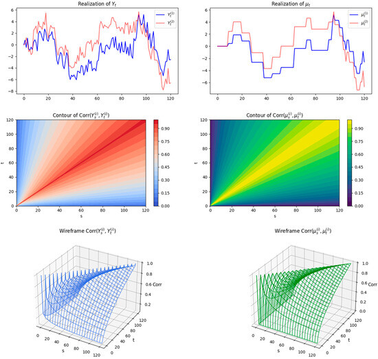
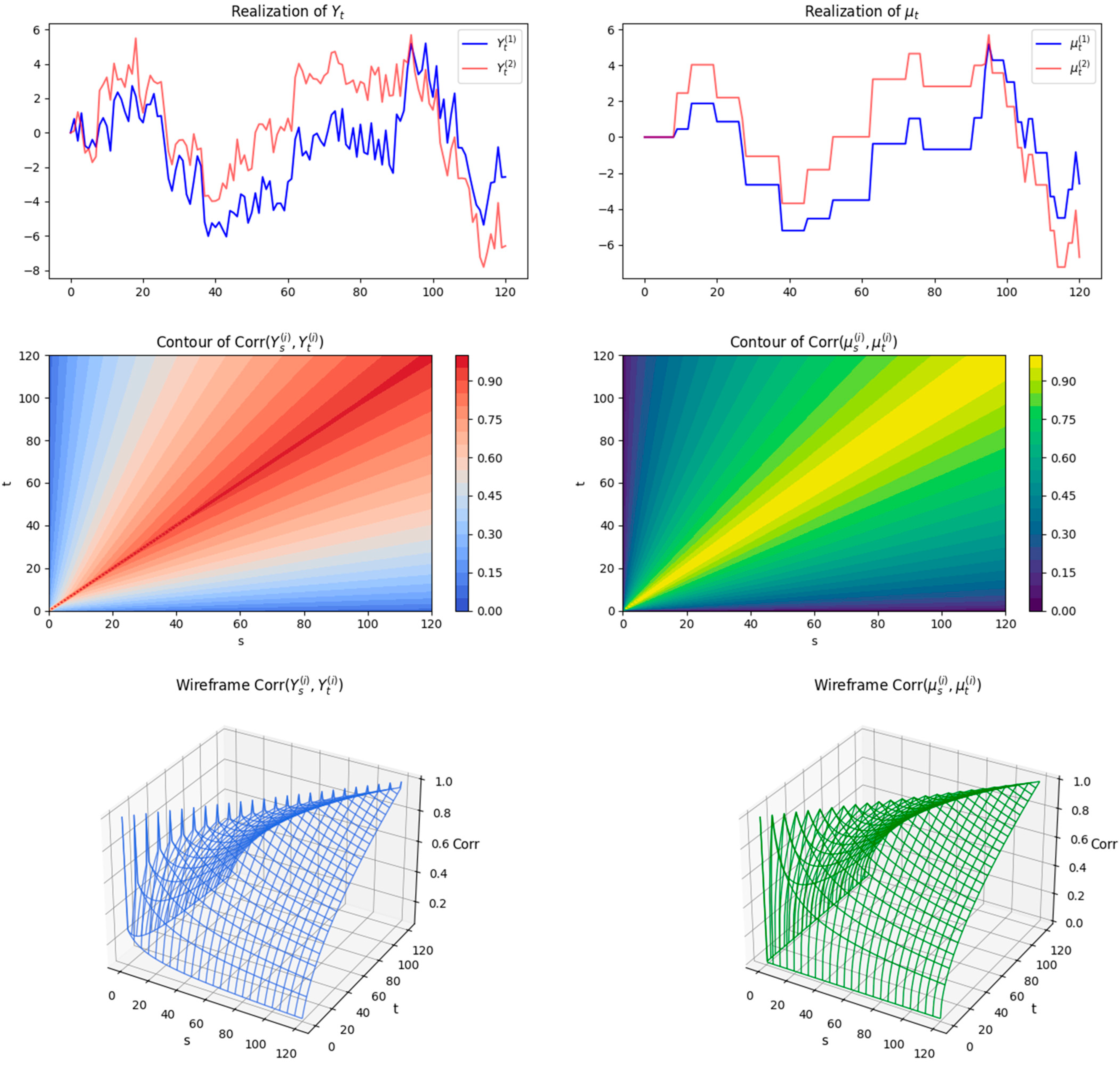
The previous theorem provides some additional insight about the stochastic structure of the 2D-GSB process. Unlike the primary GSB vector series $\left({\mathit{Y}}_{\mathit{t}}\right)$, which may exhibit sudden and pronounced fluctuations, the series $\left({\mathit{\mu }}_{\mathit{t}}\right)$ is ${\mathcal{F}}_{t-1}$ measurable and thus represents the predictable, stable component of the process, as illustrated in the upper panels of Figure 1. In contrast, the innovations $\left({\mathit{\epsilon }}_{\mathit{t}}\right)$ constitute the noise component of $\left({\mathit{Y}}_{\mathit{t}}\right)$ and represent the main source of abrupt fluctuations in the 2D-GSB framework. Moreover, according to Equations (5) and (6), the covariance matrices of both vector series $\left({\mathit{Y}}_{\mathit{t}}\right)$ and $\left({\mathit{\mu }}_{\mathit{t}}\right)$ are time-dependent and vary with $s,t\ge 0$, indicating the non-stationarity of both of these series.

Figure 1. Panels above: Dynamics of non-stationary components of the 2D-GSB process. Other panels: Autocorrelation functions of the non-stationary components (Parameter values are: $\mu =0, {\sigma }_1^2={\sigma }_1^2=1, \rho =0.6$ and $c\approx 3.8$.).

Finally, using Equations (5)–(10), the autocorrelation functions of the components of these two vector series are easily obtained as follows:

$$\begin{gathered} \mathrm{C}\mathrm{o}\mathrm{r}\mathrm{r}\left({\mu }_s^{\left(i\right)},{\mu }_t^{\left(i\right)}\right)={\displaystyle \frac{\mathrm{C}\mathrm{o}\mathrm{v}\left({\mu }_s^{\left(i\right)},{\mu }_t^{\left(i\right)}\right)}{\sqrt{\mathrm{V}\mathrm{a}\mathrm{r}\left({\mu }_s^{\left(i\right)}\right)}·\sqrt{\mathrm{V}\mathrm{a}\mathrm{r}\left({\mu }_t^{\left(i\right)}\right)}}}=\left\{\begin{array}{cc}{\displaystyle \frac{\min \left(s,t\right)}{\sqrt{s·t}}},& s\ne t\\ 1,\hfill & s=t.\end{array}\right.. \\ \mathrm{C}\mathrm{o}\mathrm{r}\mathrm{r}\left(Y_s^{\left(i\right)},Y_t^{\left(i\right)}\right)={\displaystyle \frac{\mathrm{C}\mathrm{o}\mathrm{v}\left(Y_s^{\left(i\right)},Y_t^{\left(i\right)}\right)}{\sqrt{\mathrm{V}\mathrm{a}\mathrm{r}\left(Y_s^{\left(i\right)}\right)}·\sqrt{\mathrm{V}\mathrm{a}\mathrm{r}\left(Y_t^{\left(i\right)}\right)}}}=\left\{\begin{array}{cc}{\displaystyle \frac{p_c\left(1+\min \left(s,t\right)\right)}{\sqrt{\left(1+p_{c}s\right)·\left(1+p_{c}t\right)}}},& s\ne t\\ 1,\hfill & s=t.\end{array}\right. \end{gathered}$$

It should be noted that these results are completely analogous to the results of the one-dimensional GSB process (see, e.g., Stojanović et al. [11]). Hence, the autocorrelations of the martingale mean values are L²-continuous, because

$$\underset{s\to t}{\lim } \mathrm{C}\mathrm{o}\mathrm{r}\mathrm{r}\left({\mu }_s^{\left(i\right)},{\mu }_t^{\left(i\right)}\right)={\displaystyle \frac{t}{\sqrt{t^2}}}=1,$$

while the autocorrelations of $\left({\mathit{Y}}_{\mathit{t}}\right)$ clearly do not satisfy the L²-continuity condition.

Additionally, note that autocorrelations, as well as variances, are more pronounced with series $\left({\mathit{Y}}_{\mathit{t}}\right)$, in relation to $\left({\mathit{\mu }}_{\mathit{t}}\right)$, which is a consequence of the inclusion of an additional noise term and can be seen in the lower graphs of Figure 1. Finally, using Equations (7)–(10), for the intercorrelation between the components of the above processes, one easily obtains:

$$\mathrm{C}\mathrm{o}\mathrm{r}\mathrm{r}\left({\mu }_t^{\left(1\right)},{\mu }_t^{\left(2\right)}\right)=\mathrm{C}\mathrm{o}\mathrm{r}\mathrm{r}\left(Y_t^{\left(1\right)},Y_t^{\left(2\right)}\right)=\rho .$$

Thus, both intercorrelations are constant and equal to the intercorrelations of the components of the innovations $\left({\mathit{\epsilon }}_{\mathit{t}}\right)$, regardless of time $t$. This means that all observed processes develop in the same way, i.e., they have the same intercorrelation as between the components of the innovation series.

In the following, we define another component of the 2D-GSB process, the so-called increments, as the vector series ${\mathit{X}}_{\mathit{t}}={(X_t^{\left(1\right)},X_t^{\left(2\right)})}^{\mathrm{\top }}$ which satisfies the following equalities:

$$X_t^{\left(i\right)}=Y_t^{\left(i\right)}-Y_{t-1}^{\left(i\right)}=\left({\mu }_t^{\left(i\right)}-{\mu }_{t-1}^{\left(i\right)}\right)+\left({\epsilon }_t^{\left(i\right)}-{\epsilon }_{t-1}^{\left(i\right)}\right), i=\mathrm{1,2}, t=\mathrm{1,2},\dots$$

(11)

According to Equations (3), (4) and (11), it is easy to see that the components of the vector series $\left({\mathit{X}}_{\mathit{t}}\right)$ can be presented as follows:

$$X_t^{\left(i\right)}={\epsilon }_t^{\left(i\right)}-r_{t-1}{\epsilon }_{t-1}^{\left(i\right)}, i=\mathrm{1,2}, t=\mathrm{1,2},\dots ,$$

(12)

where $r_t=1-q_t=I\left({‖{\mathit{\epsilon }}_{\mathit{t}-\mathbf{1}}‖}^2\le c\right)$. Thus, the vector series $\left({\mathit{X}}_{\mathit{t}}\right)$ is a non-linear stochastic process with random coefficient $r_t$, which is “close” to the standard moving average (MA) processes (of order 1). More precisely, the series $\left({\mathit{X}}_{\mathit{t}}\right)$ operates in two regimes:

(a)

Emphasized fluctuations of innovations $\left({\mathit{\epsilon }}_{\mathit{t}}\right)$ in the previous time moment $t-1$ imply $r_{t-1}=0$, so Equation (12) becomes $X_t^{\left(i\right)}={\epsilon }_t^{\left(i\right)}$.

(b)

Fluctuations of ${\mathit{\epsilon }}_{\mathit{t}-\mathbf{1}}$ which do not exceed the critical value $c$ imply $r_{t-1}=1$. Then, $X_t^{\left(i\right)}$ is in the form of a standard, linear MA(1) process, i.e., $X_t^{\left(i\right)}={\epsilon }_t^{\left(i\right)}-{\epsilon }_{t-1}^{\left(i\right)}$.

According to this, the vector series $\left({\mathit{X}}_{\mathit{t}}\right)$ has similar properties to the vector MA(1) models, and its stochastic properties (mean, covariance matrix, and autocorrelation function) can be obtained as given below.

Theorem 2.

Let $\left({\mathit{X}}_{\mathit{t}}\right)$ be the vector series defined by Equations (11) and (12). Then, $\left({\mathit{X}}_{\mathit{t}}\right)$ is the zero-mean vector series with the covariance matrix:

$${\Gamma }_X\left(h\right)=Cov \left({\mathit{X}}_{\mathit{t}},{\mathit{X}}_{\mathit{t}+\mathit{h}}\right)=\left\{\begin{array}{cc}\begin{array}{c}\left(2-p_c\right)·\Sigma ,\\ \left(p_c-1\right)·\Sigma ,\\ {\mathbf{0}}_{\mathbf{2}\times \mathbf{2}},\end{array}& \begin{array}{c}h=0\\ h=\pm 1\\ \left|h\right|\ge 2.\end{array}\end{array}\right.$$

(13)

In addition, the autocorrelation of the components $X_t^{\left(i\right)},$ $i=\mathrm{1,2},$ reads as follows:

$${\rho }_X\left(h\right)≔{\displaystyle \frac{Cov\left(X_t^{\left(i\right)},X_{t+h}^{\left(i\right)}\right)}{Var\left(X_t^{\left(i\right)}\right)}}=\left\{\begin{array}{cc}(\begin{array}{c}1,\\ p_c-1)/(2-p_c),\\ 0, \end{array}& \begin{array}{c}h=0\\ h=\pm 1\\ \left|h\right|\ge 2.\end{array}\end{array}\right.$$

(14)

Proof. 

According to definitions of the vector series $\left({\mathit{X}}_{\mathit{t}}\right),$ given by Equations (11) and (12), it immediately follows:

$$\mathbb{E}\left({\mathit{X}}_{\mathit{t}}\right)=\mathbb{E}\left({\mathit{\epsilon }}_{\mathit{t}}\right)-\mathbb{E}\left({r_{t-1}\mathit{\epsilon }}_{\mathit{t}-1}\right)={\mathbf{0}}_{\mathbf{2}\times \mathbf{1}}.$$

Further, similarly to the proof of the previous theorem, Equation (13) is obtained from the equalities:

$$\mathrm{C}\mathrm{o}\mathrm{v}\left(X_t^{\left(i\right)},X_{t+h}^{\left(i\right)}\right)=\mathbb{E}\left(X_t^{\left(i\right)}{X}_{t+h}^{\left(i\right)}\right)=\mathbb{E}\left[\left({\epsilon }_t^{\left(i\right)}-r_{t-1}{\epsilon }_{t-1}^{\left(i\right)}\right)\left({\epsilon }_{t+h}^{\left(i\right)}-r_{t+h-1}{\epsilon }_{t+h-1}^{\left(i\right)}\right)\right]=\left\{\begin{array}{cc}\begin{array}{c}\left(2-p_c\right){\sigma }_i^2,\\ \left(p_c-1\right){\sigma }_i^2,\\ 0,\end{array}& \begin{array}{c}h=0\\ h=\pm 1\\ \left|h\right|\ge 2\end{array}\end{array}\right.,$$

(15)

$$\mathrm{C}\mathrm{o}\mathrm{v}\left(X_t^{\left(i\right)},X_{t+h}^{\left(j\right)}\right)=\mathbb{E}\left(X_t^{\left(i\right)}{X}_{t+h}^{\left(j\right)}\right)=\mathbb{E}\left[\left({\epsilon }_t^{\left(i\right)}-r_{t-1}{\epsilon }_{t-1}^{\left(i\right)}\right)\left({\epsilon }_{t+h}^{\left(j\right)}-r_{t+h-1}{\epsilon }_{t+h-1}^{\left(j\right)}\right)\right]=\left\{\begin{array}{cc}\begin{array}{c}\left(2-p_c\right)\rho {\sigma }_1{\sigma }_2,\\ \left(p_c-1\right)\rho {\sigma }_1{\sigma }_2,\\ 0,\end{array}& \begin{array}{c}h=0\\ h=\pm 1\\ \left|h\right|\ge 2\end{array}\end{array}\right.,$$

where $i,j=\mathrm{1,2}$ and $i\ne j.$ Finally, Equations (13) and (15) directly imply Equation (14). □

Remark 2.

According to the previous theorem, it is obvious that the vector series $\left({\mathit{X}}_{\mathit{t}}\right)$ is stationary, with a structure similar to the standard MA(1) vector series. In addition, from Equations (11) and (12), it follows that

$$Y_t^{\left(i\right)}-Y_{t-1}^{\left(i\right)}={\epsilon }_t^{\left(i\right)}-r_{t-1}{\epsilon }_{t-1}^{\left(i\right)}, i=\mathrm{1,2}, t=\mathrm{1,2},\dots$$

which is a non-linear integrated auto-regressive moving average (ARIMA) model with “temporary” components $\left(r_{t-1}{\epsilon }_{t-1}^{\left(i\right)}\right)$. It implies a specific structure and distributional properties of the (stationary) series $\left({\mathit{X}}_{\mathit{t}}\right)$, as well as other (non-stationary) components of the 2D-GSB process, which is discussed in more detail below.

3. Distributional Properties

In this section, we examine selected stochastic properties of the main components of the 2D-GSB process, focusing on their distributional and asymptotic behavior. To this end, as mentioned earlier, the vector series of increments $\left({\mathit{X}}_{\mathit{t}}\right)$ plays a central role, primarily due to its stationarity. The key distributional properties of this series are summarized in the following result.

Theorem 3.

Let $q_t\left(c\right)$ be the noise indicator given by Equation (4), and $\left({\mathit{X}}_{\mathit{t}}\right)$ the bivariate time series, defined by Equations (11) and (12). Then, for any $\mathit{x}={(x_1,x_2)}^{\top }\in {\mathbb{R}}^2$ and $t=\mathrm{1,2},\dots ,$ the cumulative distribution function (CDF) of the bivariate RVs $\left({\mathit{X}}_{\mathit{t}}\right)$ is given by

$$F_{\mathit{X}}\left(\mathit{x}\right)≔P\left\{{\mathit{X}}_{\mathit{t}}<\mathit{x}\right\}=p_c{F}_1\left(\mathit{x}\right)+\left(1-p_c\right)F_2\left(\mathit{x}\right),$$

(16)

where $F_1\left(\mathit{x}\right)$ and $F_2\left(\mathit{x}\right)$ are CDFs of the bivariate Gaussian RVs ${\mathit{\epsilon }}_{\mathit{t}}~\mathcal{N}(\mathbf{0},\Sigma )$ and $\sqrt{2}{\mathit{\epsilon }}_{\mathit{t}}~\mathcal{N}\left(\mathbf{0},2\Sigma \right),$ respectively. In addition, for the series $\left({‖{\mathit{\epsilon }}_{\mathit{t}}‖}^2\right)$ the following equality (in the distribution) holds

$${‖{\mathit{\epsilon }}_{\mathit{t}}‖}^2\stackrel{d}{=}{\lambda }_1{Z}_1+{\lambda }_2{Z}_2,$$

(17)

where ${\lambda }_1,{\lambda }_2>0$ are the eigenvalues of the matrix $\Sigma$, and $Z_1,Z_2$ are the ${\chi }_1^2$ distributed RVs.

Proof. 

Using the conditional probabilities and Equation (12), for the CDF of RVs $\left({\mathit{X}}_{\mathit{t}}\right)$ one obtains

$$\begin{gathered} F_{\mathit{X}}\left(\mathbf{x}\right)≔P\left\{{\mathit{X}}_{\mathit{t}}<\mathbf{x}\right\}=P\left\{{\mathit{X}}_{\mathit{t}}<\mathbf{x}|r_{t-1}=0\right\}·P\left\{r_{t-1}=0\right\}+P\left\{{\mathit{X}}_{\mathit{t}}<\mathbf{x}|r_{t-1}=1\right\}·P\left\{r_{t-1}=1\right\} \\ =P\left\{{\mathit{\epsilon }}_{\mathit{t}}<\mathbf{x}\right\}·p_c+P\left\{{\mathit{\epsilon }}_{\mathit{t}}-{\mathit{\epsilon }}_{\mathit{t}-1}<\mathbf{x}\right\}·\left(1-p_c\right), \end{gathered}$$

which immediately implies Equation (16). Furthermore, the eigenvalues ${\lambda }_1,{\lambda }_2$ of the matrix $\Sigma \in {\mathbb{R}}^{2\times 2}$ are solutions (in terms of $\lambda )$ of the equation $\det \left(\Sigma -\lambda I\right)=0$, i.e.,

$${\lambda }^2-\left({\sigma }_1^2+{\sigma }_2^2\right)\lambda +\left(1-{\rho }^2\right){\sigma }_1^2{\sigma }_2^2=0.$$

According to the Vieta formulas, it follows that

$${\lambda }_1+{\lambda }_2={\sigma }_1^2+{\sigma }_2^2>0, {\lambda }_1{\lambda }_2=\left(1-{\rho }^2\right){\sigma }_1^2{\sigma }_2^2>0,$$

that is, ${\lambda }_1,{\lambda }_2>0.$ Hence, according to the spectral theorem (see, e.g., [18], Section 29.2.) a positive symmetric matrix $\Sigma \in {\mathbb{R}}^{2\times 2}$ has the spectral decomposition $\Sigma =P\mathsf{\Lambda }{P}^{\top }.$ Herein, $P=\left({\overrightarrow{v}}_1,{\overrightarrow{v}}_2\right)\in {\mathbb{R}}^{2\times 2}$ is an orthogonal matrix ($P{P}^{\top }=P^{\top }P=I)$ of orthonormal eigenvectors ${\overrightarrow{v}}_1,{\overrightarrow{v}}_2$ of the matrix $\Sigma$, and $\mathsf{\Lambda }=\mathrm{d}\mathrm{i}\mathrm{a}\mathrm{g}({\lambda }_1,{\lambda }_2)$ is a diagonal matrix of the eigenvalues ${\lambda }_1,{\lambda }_2$. Now, let us define a new vector series

$${\mathit{\eta }}_{\mathit{t}}=P^{\top }{\mathit{\epsilon }}_{\mathit{t}}={\left({{\overrightarrow{v}}_1}^{\top }{\mathit{\epsilon }}_{\mathit{t}}, {{\overrightarrow{v}}_2}^{\top }{\mathit{\epsilon }}_{\mathit{t}}\right)}^{\top },$$

which satisfies the equalities:

$$\begin{gathered} \mathbb{E}\left({\mathit{\eta }}_{\mathit{t}}\right)=P^{\top }\mathbb{E}\left({\mathit{\epsilon }}_{\mathit{t}}\right)={\mathbf{0}}_{\mathbf{2}\times \mathbf{1}}, \\ \mathrm{C}\mathrm{o}\mathrm{v}\left({\mathit{\eta }}_{\mathit{t}}\right)=\mathbb{E}\left({\mathit{\eta }}_{\mathit{t}}{\mathit{\eta }}_{\mathit{t}}^{\top }\right)=\mathbb{E}\left(P^{\top }{\mathit{\epsilon }}_{\mathit{t}}{\mathit{\epsilon }}_{\mathit{t}}^{\top }P\right)=P^{\top }\Sigma P=P^{\top }\left(P\mathsf{\Lambda }{P}^{\top }\right)P=\mathsf{\Lambda }. \end{gathered}$$

Thus, ${\mathit{\eta }}_{\mathit{t}}=\left({\eta }_t^{\left(1\right)},{\eta }_t^{\left(2\right)}\right)$ is a bivariate Gaussian process, with ${\eta }_t^{\left(i\right)}~\mathcal{N}\left(0,{\lambda }_i\right),$ $i=\mathrm{1,2},$ and ${\eta }_t^{\left(1\right)}\perp {\eta }_t^{\left(2\right)}.$ Finally, Equation (17) follows from ${\mathit{\epsilon }}_{\mathit{t}}=P{\mathit{\eta }}_{\mathit{t}}$ and the equalities:

$${‖{\mathit{\epsilon }}_{\mathit{t}}‖}^2={\mathit{\epsilon }}_{\mathit{t}}^{\top }{{\mathit{\epsilon }}_{\mathit{t}}=\mathit{\eta }}_{\mathit{t}}^{\top }{P}^{\top }P{\mathit{\eta }}_{\mathit{t}}={{\mathsf{\eta }}_{\mathbf{t}}}^{\top }{\mathsf{\eta }}_{\mathbf{t}}={‖{\mathit{\eta }}_{\mathit{t}}‖}^2.$$

□

Remark 3.

Similar to the one-dimensional case of the GSB process (see, e.g., Jovanović et al. [12]), by differentiating Equation (16), the bivariate probability density function (PDF) of the vector series $\left({\mathit{X}}_{\mathit{t}}\right)$ can be obtained as follows:

$$f_X\left(\mathbf{x}\right)=p_c{f}_1\left(\mathbf{x}\right)+\left(1-p_c\right)f_2\left(\mathbf{x}\right).$$

Here,

$$f_k\left(\mathbf{x}\right)={\displaystyle \frac{1}{2\pi \sqrt{\det \Sigma }}}\exp \left(-{\displaystyle \frac{1}{2}}{\mathbf{x}}^{\mathit{\top }}{\left(k\Sigma \right)}^{-1}\mathbf{x}\right), k=\mathrm{1,2}$$

are the bivariate PDFs of the Gaussian distributions $\mathcal{N}({\mathbf{0}}_{\mathbf{2}\times \mathbf{1}},k\Sigma )$, where $k=\mathrm{1,2}.$ Thus, the distribution of increments $\left({\mathit{X}}_{\mathit{t}}\right)$ is a convex linear combination (i.e., mixture) of two known 2D normal distributions with zero mean and different variance–covariance matrices. In the same way, using standard procedures, for the bivariate CF of the vectors $\left({\mathit{X}}_{\mathit{t}}\right)$ one obtains

$$\begin{gathered} {\phi }_{\mathit{X}}\left(\mathbf{u}\right)=\mathbb{E}\left(\exp \mathrm{i}⟨\mathbf{u},{\mathit{X}}_{\mathit{t}}⟩\right)=p_c{\phi }_{\epsilon }\left(\mathbf{u}\right)+\left(1-p_c\right){\phi }_{\sqrt{2}\epsilon }\left(\mathbf{u}\right) \\ =p_c\exp \left(-{\displaystyle \frac{1}{2}}{\mathbf{u}}^{\mathit{\top }}\Sigma \mathbf{u}\right)+\left(1-p_c\right)\exp \left(-{\mathbf{u}}^{\mathit{\top }}\Sigma \mathbf{u}\right), \end{gathered}$$

(18)

where $\mathit{u}={(u_1,u_2)}^{\mathit{\top }}\in {\mathbb{R}}^2$ and ${\phi }_{\epsilon }\left(\mathit{u}\right)=\mathit{exp}\left(-{\mathit{u}}^{\mathit{\top }}\Sigma \mathit{u}/2\right)$ is the CF of the bivariate Gaussian RVs  $\left({\mathit{\epsilon }}_{\mathit{t}}\right)~\mathcal{N}\left(\mathbf{0},\Sigma \right).$

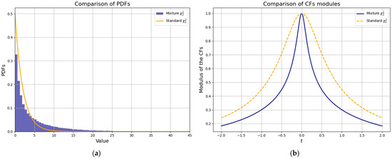
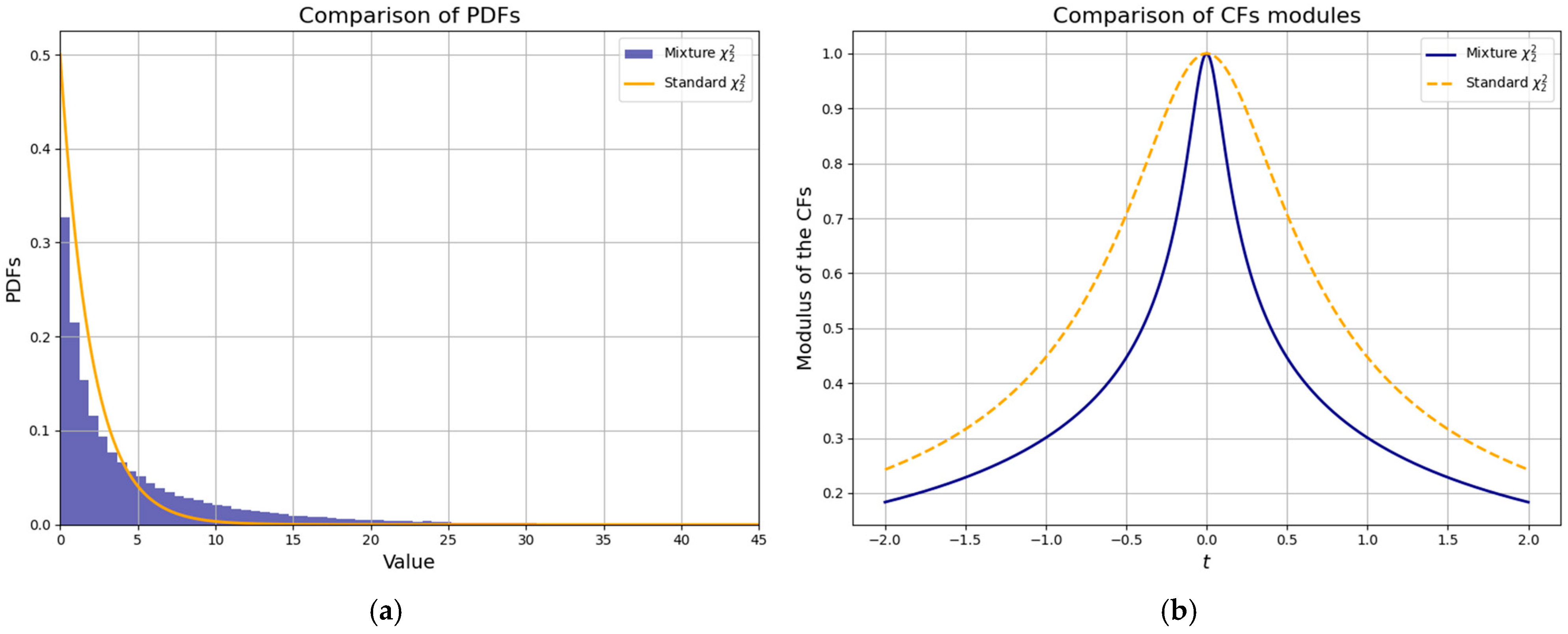
On the other hand, Equation (17) indicates that RVs ${\zeta }_t={‖{\mathit{\epsilon }}_{\mathit{t}}‖}^2$ have the so-called weighted (i.e., mixture) ${\chi }_2^2$ distribution. In general, the distribution of $\left({\zeta }_t\right)$ differs from the “ordinary” chi-square distribution (see Figure 2) and does not have a closed form for its PDF and CDF. Nevertheless, it is easy to see that the CF of this distribution is of the form

$${\phi }_{\zeta }\left(u\right)=\mathbb{E}\left(\exp \left(\mathrm{i}u({\lambda }_1{Z}_1+{\lambda }_2{Z}_2)\right)\right)={\phi }_{{\mathit{Z}}_1}\left({\lambda }_{1}u\right){\phi }_{{\mathit{Z}}_2}\left({\lambda }_{2}u\right)={\left(\left(1-2\mathrm{i}{\lambda }_{1}u\right)\left(1-2\mathrm{i}{\lambda }_{2}u\right)\right)}^{-1/2},$$

where $u\in \mathbb{R}.$ This fact, along with Equation (18), can be useful in estimating the parameters of the 2D-GSB model, as discussed below.

Figure 2. Comparison of PDF (a) and CF moduli (b) of weighted and standard ${\chi }_2^2$ distribution. (Parameter values are: ${\sigma }_1=1, {\sigma }_2=2$ and $\rho =0.8$, which imply ${\lambda }_1\approx 0.307, {\lambda }_2\approx 4.693$).

The distribution of bivariate series $\left({\mathit{\mu }}_{\mathit{t}}\right)$ and $\left({\mathit{Y}}_{\mathit{t}}\right),$ as non-stationary components of the GSB process, can be described as follows.

Theorem 4.

Let $\left({\mathit{Y}}_{\mathit{t}}\right)$ and $\left({\mathit{\mu }}_{\mathit{t}}\right)$ be the bivariate time series defined, respectively, by Equations (1) and (3), where ${\mathit{\mu }}_0\stackrel{as}{=}{(m_1,m_2)}^{\top } \left(const\right).$ Then, for any $\mathit{x}={(x_1,x_2)}^{\top } \in {\mathbb{R}}^2$ and $t=\mathrm{0,1},2,\dots$, the CDFs of these series are

$$F_{\mu }\left(\mathit{x},t\right)≔P\left\{{\mathit{\mu }}_{\mathit{t}}<\mathit{x}\right\}=\sum _{k=0}^t{\pi }_k^{\left(t\right)}\left(c\right)F_k\left(\mathit{x}\right), F_Y\left(\mathit{x},t\right)≔P\left\{{\mathit{Y}}_{\mathit{t}}<\mathit{x}\right\}=\sum _{k=0}^t{\pi }_k^{\left(t\right)}\left(c\right)F_{k+1}\left(\mathit{x}\right),$$

(19)

where ${\pi }_k^{\left(t\right)}\left(c\right)≔\left({\displaystyle \genfrac{}{}{0pt}{}{t}{k}}\right)p_c^k{\left(1-p_c\right)}^{t-k}$ and $F_k\left(\mathit{x}\right),$ $k=0,\dots ,t$ are the CDFs of the bivariate Gaussian RVs $\mathcal{N}({\mathit{\mu }}_{\mathbf{0}},k\Sigma )$. Furthermore, the following convergences (in distribution) hold:

$$t^{-1/2}{\mathit{\mu }}_{\mathit{t}}\stackrel{d}{⟶}\mathcal{N}\left(\mathbf{0},p_c\Sigma \right), t^{-1/2}{\mathit{Y}}_{\mathit{t}}\stackrel{d}{⟶}\mathcal{N}\left(\mathbf{0},p_c\Sigma \right), t\to +\infty .$$

(20)

Proof. 

Let us define the bivariate RVs ${\mathit{\xi }}_{\mathit{t}}=q_t{\mathit{\epsilon }}_{\mathit{t}}$, where $t=0,1,\dots$ It can be easily proven that $\left({\mathit{\xi }}_{\mathit{t}}\right)$ is a series of mutually uncorrelated RVs, with $E\left({\mathit{\xi }}_{\mathit{t}}\right)={\mathbf{0}}_{\mathbf{2}\times \mathbf{1}}$ and $\mathrm{C}\mathrm{o}\mathrm{v}\left({\mathit{\xi }}_{\mathit{t}}\right)=p_c\Sigma$. By reapplying conditional probabilities, the CDF of RVs $\left({\mathit{\xi }}_{\mathit{t}}\right)$ is obtained as

$$\begin{gathered} F_{\xi }\left(\mathbf{x}\right)≔P\left\{{\mathit{\xi }}_{\mathit{t}}<\mathbf{x}\right\}=P\left\{{\mathit{\xi }}_{\mathit{t}}<\mathbf{x}|q_t=1\right\}·P\left\{q_t=1\right\}+P\left\{{\mathit{\xi }}_{\mathit{t}}<\mathbf{x}|q_t=0\right\}·P\left\{q_t=0\right\} \\ =P\left\{{\mathit{\epsilon }}_{\mathit{t}}<\mathbf{x}\right\}·p_c+P\left\{\mathbf{0}<\mathbf{x}\right\}·\left(1-p_c\right)=p_c{F}_{\epsilon }\left(\mathbf{x}\right)+\left(1-p_c\right)F_{\mathsf{\delta }}\left(\mathbf{x}\right), \end{gathered}$$

where $F_{\mathsf{\delta }}\left(\mathbf{x}\right)=I\left(\mathbf{x}>\mathbf{0}\right)$ is the CDF of the bivariate RV ${\mathit{\delta }}_{\mathbf{0}}\stackrel{as}{=}\mathbf{0}.$ According to this, for the CF of the RVs $\left({\mathit{\xi }}_{\mathit{t}}\right)$ one obtains

$${\phi }_{\xi }\left(\mathbf{u}\right)=E\left(\exp i⟨\mathbf{u},{\mathit{\xi }}_{\mathit{t}}⟩\right)=p_c{\phi }_{\epsilon }\left(\mathbf{u}\right)+\left(1-p_c\right){\phi }_{\mathsf{\delta }}\left(\mathbf{u}\right)=p_c\exp \left(-{\displaystyle \frac{1}{2}}{\mathbf{u}}^{\mathit{T}}\mathbf{\Sigma }\mathbf{u}\right)+(1-p_c),$$

where ${\phi }_{\delta }\left(u\right)\equiv 1$ is the CF of the RV ${\mathit{\delta }}_{\mathbf{0}}$. Now, by applying Equation (3), for the CFs of the martingale means $\left({\mathit{\mu }}_{\mathit{t}}\right)$ we get

$$\begin{gathered} {\phi }_{\mu }\left(\mathbf{u},t\right)=E\left(\exp \mathrm{i}⟨\mathbf{u},{\mathit{\mu }}_{\mathit{t}}⟩\right)=\exp \left(\mathrm{i}⟨\mathbf{u},{\mathit{\mu }}_0⟩\right)E\left(\prod _{s=0}^{t-1}\exp \left(\mathrm{i}{q}_s⟨\mathbf{u},{\mathit{\epsilon }}_{\mathit{s}}⟩\right)\right) \\ =\exp \left(\mathrm{i}{\mathbf{u}}^{\mathit{\top }}{\mathit{\mu }}_0\right){\left(p_c\exp \left(-{\displaystyle \frac{1}{2}}{\mathbf{u}}^{\mathit{\top }}\mathbf{\Sigma }\mathbf{u}\right)+\left(1-p_c\right)\right)}^t \\ =\exp \left(\mathrm{i}{\mathbf{u}}^{\mathit{\top }}{\mathit{\mu }}_0\right){\sum }_{k=0}^t\left({\displaystyle \genfrac{}{}{0pt}{}{t}{k}}\right)p_c^k{\left(1-p_c\right)}^{t-k}\exp \left(-{\displaystyle \frac{1}{2}}k{\mathbf{u}}^{\mathit{\top }}\mathbf{\Sigma }\mathbf{u}\right), \end{gathered}$$

(21)

where the binomial formula is used in the last equality. From here, by applying Lévy’s correspondence theorem (see, e.g., [19], Section 14.2), the first part of Equation (19) immediately follows. Similarly, using Equations (1) and (21), for the CFs of series $\left({\mathit{Y}}_{\mathit{t}}\right)$ one obtains:

$$\begin{gathered} {\phi }_Y\left(\mathbf{u},t\right)=E\left(\exp \mathrm{i}⟨\mathbf{u},{\mathit{Y}}_{\mathit{t}}⟩\right)={\phi }_{\mu }\left(\mathbf{u},t\right)·{\phi }_{\epsilon }\left(\mathbf{u}\right) \\ =\exp \left(\mathrm{i}{\mathbf{u}}^{\mathit{\top }}{\mathit{\mu }}_0\right){\left(p_c\exp \left(-{\displaystyle \frac{1}{2}}{\mathbf{u}}^{\mathit{\top }}\mathbf{\Sigma }\mathbf{u}\right)+\left(1-p_c\right)\right)}^{t}E\left(\exp \left(\mathrm{i}⟨\mathbf{u},{\mathit{\epsilon }}_{\mathit{t}}⟩\right)\right) \\ =\exp \left(\mathrm{i}{\mathbf{u}}^{\mathit{\top }}{\mathit{\mu }}_0-{\displaystyle \frac{1}{2}}{\mathbf{u}}^{\mathit{\top }}\mathbf{\Sigma }\mathbf{u}\right)\sum _{k=0}^t\left({\displaystyle \genfrac{}{}{0pt}{}{t}{k}}\right)p_c^k{\left(1-p_c\right)}^{t-k}\exp \left(-{\displaystyle \frac{1}{2}}k{\mathbf{u}}^{\mathit{\top }}\mathbf{\Sigma }\mathbf{u}\right) \\ =\exp \left(\mathrm{i}{\mathbf{u}}^{\mathit{\top }}{\mathit{\mu }}_{\mathbf{0}}\right){\sum }_{k=0}^t\left({\displaystyle \genfrac{}{}{0pt}{}{t}{k}}\right)p_c^k{\left(1-p_c\right)}^{t-k}\exp \left(-{\displaystyle \frac{1}{2}}(k+1){\mathbf{u}}^{\mathit{\top }}\mathbf{\Sigma }\mathbf{u}\right). \end{gathered}$$

(22)

Thus, by reapplying Lévy’s theorem, we get the second equation in (19).

To prove the second part of the theorem, i.e., Equation (20), note that the CFs of the bivariate RVs $t^{-1/2}{\mathit{\mu }}_{\mathit{t}}$ and $t^{-1/2}{\mathit{Y}}_{\mathit{t}}$, $t=1,2,\dots ,$ according to previous Equations (21) and (22), can be written as follows:

$$\begin{gathered} {\phi }_{\mu }\left(t^{-1/2}\mathbf{u},t\right)=\exp \left({\displaystyle \frac{\mathrm{i}{\mathbf{u}}^{\mathit{\top }}{\mathit{\mu }}_{\mathbf{0}}}{\sqrt{t}}}\right){\left(1+p_c\left(\exp \left(-{\displaystyle \frac{1}{2t}}{\mathbf{u}}^{\mathit{\top }}\mathbf{\Sigma }\mathbf{u}\right)-1\right)\right)}^t, \\ {\phi }_Y\left(t^{-1/2}\mathbf{u},t\right)=\exp \left({\displaystyle \frac{\mathrm{i}{\mathbf{u}}^{\mathit{\top }}{\mathit{\mu }}_{\mathbf{0}}}{\sqrt{t}}}\right){\left(1+p_c\left(\exp \left(-{\displaystyle \frac{1}{2t}}{\mathbf{u}}^{\mathit{\top }}\mathbf{\Sigma }\mathbf{u}\right)-1\right)\right)}^t\exp \left(-{\displaystyle \frac{1}{2t}}{\mathbf{u}}^{\mathit{\top }}\mathbf{\Sigma }\mathbf{u}\right). \end{gathered}$$

After taking the logarithm and developing the exponential terms, when $t\to +\mathrm{\infty }$, we get

$$\begin{gathered} \log {\phi }_{\mu }\left(t^{-1/2}\mathbf{u},t\right)={\displaystyle \frac{\mathrm{i}{\mathbf{u}}^{\mathit{\top }}{\mathit{\mu }}_{\mathbf{0}}}{\sqrt{t}}}+t\log \left(1+p_c\left(\exp \left(-{\displaystyle \frac{1}{2t}}{\mathbf{u}}^{\mathit{\top }}\mathbf{\Sigma }\mathbf{u}\right)-1\right)\right)={\displaystyle \frac{\mathrm{i}{\mathbf{u}}^{\mathit{\top }}{\mathit{\mu }}_{\mathbf{0}}}{\sqrt{t}}}-{\displaystyle \frac{p_c}{2}}{\mathbf{u}}^{\mathit{\top }}\mathbf{\Sigma }\mathbf{u}+\mathcal{O}\left(t^{-2}\right), \\ \log {\phi }_Y\left(t^{-1/2}\mathbf{u},t\right)=\log {\phi }_{\mu }\left(t^{-1/2}\mathbf{u},t\right)-{\displaystyle \frac{{\mathbf{u}}^{\mathit{\top }}\mathbf{\Sigma }\mathbf{u}}{2t}}={\displaystyle \frac{\mathrm{i}{\mathbf{u}}^{\mathit{\top }}{\mathit{\mu }}_0}{\sqrt{t}}}-{\displaystyle \frac{p_c}{2}}{\mathbf{u}}^{\mathit{\top }}\mathbf{\Sigma }\mathbf{u}-{\displaystyle \frac{1}{2t}}{\mathbf{u}}^{\mathit{\top }}\mathbf{\Sigma }\mathbf{u}+\mathcal{O}\left(t^{-2}\right), \end{gathered}$$

whence it follows:

$$\underset{t\to +\mathrm{\infty }}{\lim }{\phi }_{\mu }\left(t^{-1/2}\mathbf{u},t\right)=\underset{t\to +\mathrm{\infty }}{\lim }{\phi }_Y\left(t^{-1/2}\mathbf{u},t\right)=\exp \left(-{\displaystyle \frac{p_c}{2}}{\mathbf{u}}^{\mathit{\top }}\mathbf{\Sigma }\mathbf{u}\right).$$

Obviously, the limit thus obtained is the CF of the bivariate Gaussian distribution $\mathcal{N}\left(\mathbf{0},p_c\Sigma \right)$, which confirms both convergences in Equation (20). □

Remark 4.

Note that, based on the previous results, the CFs of both processes $\left({\mathit{\mu }}_{\mathit{t}}\right)$ and $\left({\mathit{Y}}_{\mathit{t}}\right)$ are the convex combinations (mixtures) of those Gaussian CFs with binomial weights. Due to this, the noise indicators $q_t~Bernoulli\left(p_c\right)$, $t=\mathrm{1,2},\dots$, are the mutually independent Bernoulli RVs, which implies:

$$K_t≔\sum _{s=1}^t{q}_s~Binomial\left(t,p_c\right).$$

Thus, according to Equation (19), it follows that, conditionally on $K_t=k$, both processes $\left({\mathit{\mu }}_{\mathit{t}}\right)$ and $\left({\mathit{Y}}_{\mathit{t}}\right)$ are Gaussian:

$${\mathit{\mu }}_{\mathit{t}}\left|\left(K_t=k\right)\right.~\mathcal{N}\left({\mathit{\mu }}_{\mathbf{0}},k\Sigma \right), {\mathit{Y}}_{\mathit{t}}\left|\left(K_t=k\right)\right.~\mathcal{N}\left({\mathit{\mu }}_{\mathbf{0}},(k+1)\Sigma \right).$$

Consequently, their marginals are finite Gaussian mixtures with binomial weights:

$${\mathit{\mu }}_{\mathit{t}}~\sum _{k=0}^t\left({\displaystyle \genfrac{}{}{0pt}{}{t}{k}}\right)p_c^k{\left(1-p_c\right)}^{t-k}\mathcal{N}\left({\mathit{\mu }}_{\mathbf{0}},k\Sigma \right), {\mathit{Y}}_{\mathit{t}}~\sum _{k=0}^t\left({\displaystyle \genfrac{}{}{0pt}{}{t}{k}}\right)p_c^k{\left(1-p_c\right)}^{t-k}\mathcal{N}\left({\mathit{\mu }}_{\mathbf{0}},(k+1)\Sigma \right).$$

This representation explicitly reveals the latent binomial–Gaussian mixture structure underlying the non-stationary processes $\left({\mathit{\mu }}_{\mathit{t}}\right)$ and $\left({\mathit{Y}}_{\mathit{t}}\right)$. Moreover, Equation (20) shows that even these non-stationary bivariate series $\left({\mathit{\mu }}_{\mathit{t}}\right)$ and $\left({\mathit{Y}}_{\mathit{t}}\right)$ generate asymptotic normal scaled processes $\left(t^{-1/2}{\mathit{\mu }}_{\mathit{t}}\right)$ and $\left(t^{-1/2}{\mathit{Y}}_{\mathit{t}}\right)$ as $t\to +\infty$. This behavior reflects a specific form of random thinning of bivariate Gaussian noise $\left({\mathit{\epsilon }}_{\mathit{t}}\right)$, where each innovation is incorporated into the cumulative dynamics with probability $p_c$. In the limit, the resulting distribution remains Gaussian, but with a reduced covariance matrix $p_c\Sigma$. This property is particularly relevant for practical application of the 2D-GSB process and is illustrated in Figure 3, which shows the convergence of the moduli of the CFs of $\left({\mathit{\mu }}_{\mathit{t}}\right)$ and $\left({\mathit{Y}}_{\mathit{t}}\right)$ for increasing time indices.

Figure 3. Modulus convergence of CFs for bivariate RVs $t^{-1/2}{\mathit{\mu }}_{\mathit{t}}$ (a) and $t^{-1/2}{\mathit{Y}}_{\mathit{t}}$ (b), when $t=1, 2, \dots , 50$ (Parameter values are: $p_c=0.4, {\sigma }_1={\sigma }_2=1$ and $\rho =0.6$).

Similar to the one-dimensional case, some additional asymptotic properties of the non-stationary bivariate series $\left({\mathit{\mu }}_{\mathit{t}}\right)$ and $\left({\mathit{Y}}_{\mathit{t}}\right)$ can be described in terms of their (linear) transformations. This refers to the so-called scaled averages, which provide the possibility of finding convergences in the distribution and asymptotically normal (AN) distributions. In that sense, the following statement, named the central limit theorem (CLT) of the 2D-GSB process, can be formulated:

Theorem 5.

For arbitrary $\alpha \ge 1,$ let us define the so-called $\alpha$-mean series

$${\mathit{M}}_{\mathit{t};\mathit{\alpha }}={\displaystyle \frac{1}{t^{\alpha }}}\sum _{s=1}^t{\mathit{\mu }}_{\mathit{s}}, {\mathit{U}}_{\mathit{t};\mathit{\alpha }}={\displaystyle \frac{1}{t^{\alpha }}}\sum _{s=1}^t{\mathit{Y}}_{\mathit{s}},$$

where $\left({\mathit{Y}}_{\mathit{t}}\right)$ and $\left({\mathit{\mu }}_{\mathit{t}}\right)$ are the non-stationary bivariate time series defined by Equations (1) and (3), respectively. Then, the following statements hold:

(i) 

When $1\le \alpha \le 3/2,$ the time series ${\mathit{M}}_{\mathit{t};\mathit{\alpha }}$ and ${\mathit{Y}}_{\mathit{t};\mathit{\alpha }}$ are asymptotically normally distributed, i.e., the following relations, when $t\to +\infty$ , hold:

$${\mathit{M}}_{\mathit{t};\mathit{\alpha }}~\mathcal{N}\left({\mathit{\mu }}_{\mathbf{0}}{t}^{1-\alpha },{\displaystyle \frac{p_c}{3}}{t}^{3-2\alpha }\Sigma \right), {\mathit{U}}_{\mathit{t};\mathit{\alpha }}~\mathcal{N}\left({\mathit{\mu }}_{\mathbf{0}}{t}^{1-\alpha },\left(t^{1-2\alpha }+{\displaystyle \frac{p_c}{3}}{t}^{3-2\alpha }\right)\Sigma \right).$$

(23)

(ii) 

When $\alpha >3/2,$ the time series ${\mathit{M}}_{\mathit{t};\mathit{\alpha }}$ and ${\mathit{Y}}_{\mathit{t};\mathit{\alpha }}$ asymptotically vanish, i.e.,

$${\mathit{M}}_{\mathit{t};\mathit{\alpha }}\stackrel{d}{⟶}{\mathit{\delta }}_{\mathbf{0}}, {\mathit{U}}_{\mathit{t};\mathit{\alpha }}\stackrel{d}{⟶}{\mathit{\delta }}_{\mathbf{0}}, t\to +\infty .$$

(24)

Proof. 

First, we shall prove the statement of the theorem for the bivariate series $\left({\mathit{M}}_{\mathit{t};\mathit{\alpha }}\right)$. According to the definition of the series $\left({\mathit{\mu }}_{\mathit{t}}\right)$ and $\left({\mathit{M}}_{\mathit{t};\mathit{\alpha }}\right),$ one obtains:

$${\mathit{M}}_{\mathit{t};\mathit{\alpha }}={\displaystyle \frac{1}{t^{\alpha }}}\sum _{s=1}^t{\mathit{\mu }}_{\mathit{s}}={\displaystyle \frac{1}{t^{\alpha }}}\sum _{s=1}^t\left({\mathit{\mu }}_{\mathbf{0}}+\sum _{k=0}^{s-1}{q}_k{\mathit{\epsilon }}_{\mathit{k}}\right)={\displaystyle \frac{1}{t^{\alpha }}}\left(t{\mathit{\mu }}_{\mathbf{0}}+\sum _{s=1}^t\sum _{k=0}^{s-1}{\mathit{\xi }}_{\mathit{k}}\right)=t^{1-\alpha }{\mathit{\mu }}_{\mathbf{0}}+\sum _{k=1}^t{\displaystyle \frac{k}{t^{\alpha }}}{\mathit{\xi }}_{\mathit{t}-\mathit{k}}.$$

Thus, the bivariate series $\left({\mathit{M}}_{\mathit{t};\mathit{\alpha }}\right)$ is a sum of uncorrelated bivariate RVs ${\mathit{\mu }}_{\mathbf{0}}$ and ${\mathit{\xi }}_{\mathit{s}}=q_s{\mathit{\epsilon }}_{\mathit{s}}$, $s=0,\dots , t-1$, so the CFs of $\left({\mathit{M}}_{\mathit{t};\mathit{\alpha }}\right)$ can be obtained as follows:

$${\phi }_M\left(\mathbf{u},t,\alpha \right)={\phi }_{\mu }\left(t^{1-\alpha }{\mathit{\mu }}_{\mathbf{0}},0\right)\prod _{k=1}^t{\phi }_{\xi }\left({\displaystyle \frac{k}{t^{\alpha }}}\mathbf{u}\right)=\exp \left(\mathrm{i}{t}^{1-\alpha }{\mathbf{u}}^{\mathit{\top }}{\mathit{\mu }}_0\right)\prod _{k=1}^t\left[1+p_c\left(\exp \left(-{\displaystyle \frac{k^2}{2t^{2\alpha }}}{\mathbf{u}}^{\mathit{\top }}\mathbf{\Sigma }\mathbf{u}\right)-1\right)\right].$$

Taking the logarithm of the CFs ${\phi }_M\left(\mathbf{u},t,\alpha \right)$ gives a function

$${\psi }_M\left(\mathbf{u},t,\alpha \right)≔\log {\phi }_M\left(\mathbf{u},t,\alpha \right)=\mathrm{i}{t}^{1-\alpha }{\mathbf{u}}^{\mathit{\top }}{\mathit{\mu }}_{\mathbf{0}}+\sum _{k=1}^t\log \left[1+p_c\left(\exp \left(-{\displaystyle \frac{k^2}{2t^{2\alpha }}}{\mathbf{u}}^{\mathit{\top }}\mathbf{\Sigma }\mathbf{u}\right)-1\right)\right],$$

and similarly to the previous theorem, taking its asymptotic value when $t\to +\infty ,$ we get:

$$\begin{gathered} {\psi }_M\left(\mathbf{u},t,\alpha \right)=\mathrm{i}{t}^{1-\alpha }{\mathbf{u}}^{\mathit{T}}{\mathit{\mu }}_{\mathbf{0}}-{\displaystyle \frac{p_c}{2t^{2\alpha }}}\sum _{k=1}^t{k}^2{\mathbf{u}}^{\mathit{\top }}\mathbf{\Sigma }\mathbf{u}+\mathcal{O}\left(t^{3-2\alpha }\right)=\mathrm{i}{t}^{1-\alpha }{\mathbf{u}}^{\mathit{\top }}{\mathit{\mu }}_{\mathbf{0}}-{\displaystyle \frac{p_{c}t\left(t+1\right)\left(2t+1\right)}{12t^{2\alpha }}}{\mathbf{u}}^{\mathit{\top }}\mathbf{\Sigma }\mathbf{u}+\mathcal{O}\left(t^{3-2\alpha }\right) \\ =\mathrm{i}{t}^{1-\alpha }{\mathbf{u}}^{\mathit{\top }}{\mathit{\mu }}_{\mathbf{0}}-{\displaystyle \frac{p_c{t}^{3-2\alpha }}{6}}{\mathbf{u}}^{\mathit{\top }}\mathbf{\Sigma }\mathbf{u}+\mathcal{O}\left(t^{3-2\alpha }\right)\approx \left\{\begin{array}{cc}\mathrm{i}{t}^{1-\alpha }{\mathbf{u}}^{\mathit{\top }}{\mathit{\mu }}_{\mathbf{0}}-{\displaystyle \frac{p_c{t}^{3-2\alpha }}{6}}{\mathbf{u}}^{\mathit{\top }}\mathbf{\Sigma }\mathbf{u},& 1\le \alpha \le 3/2\\ 0,& \alpha >3/2.\end{array}\right. \end{gathered}$$

By substituting the last term in the CFs ${\phi }_M\left(\mathbf{u},t,\alpha \right)$ and applying Lévy’s correspondence theorem, the first relations in Equations (23) and (24) are easily obtained.

The proof for the series ${\mathit{U}}_{\mathit{t};\mathsf{\alpha }}$ can be carried out in an analogous way. Using Equation (1), as well as the previously proven facts, we have that

$${\mathit{U}}_{\mathit{t};\mathit{\alpha }}=t^{-\alpha }\sum _{j=1}^t\left({\mathit{\mu }}_{\mathit{j}}+{\mathit{\epsilon }}_{\mathit{j}}\right)={\mathit{M}}_{\mathit{t};\mathit{\alpha }}+t^{-\alpha }\sum _{j=1}^t{\mathit{\epsilon }}_{\mathit{j}},$$

where $t^{-\alpha }\sum _{j=1}^t{\mathit{\epsilon }}_{\mathit{j}}~\mathcal{N}\left(\mathbf{0},t^{1-2\alpha }\Sigma \right).$ From here, for the CFs of the series $\left({\mathit{U}}_{\mathit{t};\mathit{\alpha }}\right)$ one obtains:

$$\begin{gathered} {\phi }_U\left(\mathbf{u},t,\alpha \right)={\phi }_M\left(\mathbf{u},t,\alpha \right)\prod _{j=1}^t{\phi }_{\epsilon }\left(t^{-\alpha }\mathbf{u}\right) \\ =\exp \left(\mathrm{i}{t}^{1-\alpha }{\mathbf{u}}^{\mathit{T}}{\mathit{\mu }}_{\mathbf{0}}\right)\exp \left(-{\displaystyle \frac{t^{1-2\alpha }}{2}}{\mathbf{u}}^{\mathit{T}}\mathbf{\Sigma }\mathbf{u}\right)\prod _{k=1}^t\left[1+p_c\left(\exp \left(-{\displaystyle \frac{k^2}{2t^{2\alpha }}}{\mathbf{u}}^{\mathit{T}}\mathbf{\Sigma }\mathbf{u}\right)-1\right)\right]. \end{gathered}$$

Using a similar procedure as in the previous part of the proof, i.e., taking the logarithm of the function ${\phi }_U\left(\mathbf{u},t,\mathsf{\alpha }\right),$ we get

$${\psi }_U\left(\mathbf{u},t,\alpha \right)≔\log {\phi }_U\left(\mathbf{u},t,\alpha \right)=\mathrm{i}{t}^{1-\alpha }{\mathbf{u}}^{\mathit{T}}{\mathit{\mu }}_{\mathbf{0}}-{\displaystyle \frac{t^{1-2\alpha }}{2}}{\mathbf{u}}^{\mathit{T}}\mathbf{\Sigma }\mathbf{u}+\sum _{k=1}^t\log \left[1+p_c\left(\exp \left(-{\displaystyle \frac{k^2}{2t^{2\alpha }}}{\mathbf{u}}^{\mathit{T}}\mathbf{\Sigma }\mathbf{u}\right)-1\right)\right],$$

and by taking asymptotic value when $t\to +\infty$, it follows:

$${\psi }_U\left(\mathbf{u},t,\alpha \right)\approx \left\{\begin{array}{cc}\mathrm{i}{t}^{1-\alpha }{\mathbf{u}}^{\mathit{T}}{\mathit{\mu }}_{\mathbf{0}}-\left({\displaystyle \frac{t^{1-2\alpha }}{2}}+{\displaystyle \frac{p_c{t}^{3-2\alpha }}{6}}\right){\mathbf{u}}^{\mathit{T}}\mathbf{\Sigma }\mathbf{u},& 1\le \alpha \le 3/2\\ 0,& \alpha >3/2.\end{array}\right.$$

Therefore, by substituting this expression into the CFs ${\phi }_U\left(\mathbf{u},t,\alpha \right)$, the second relations in Equations (23) and (24) are obtained, which fully proves the theorem. □

Remark 5.

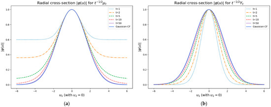
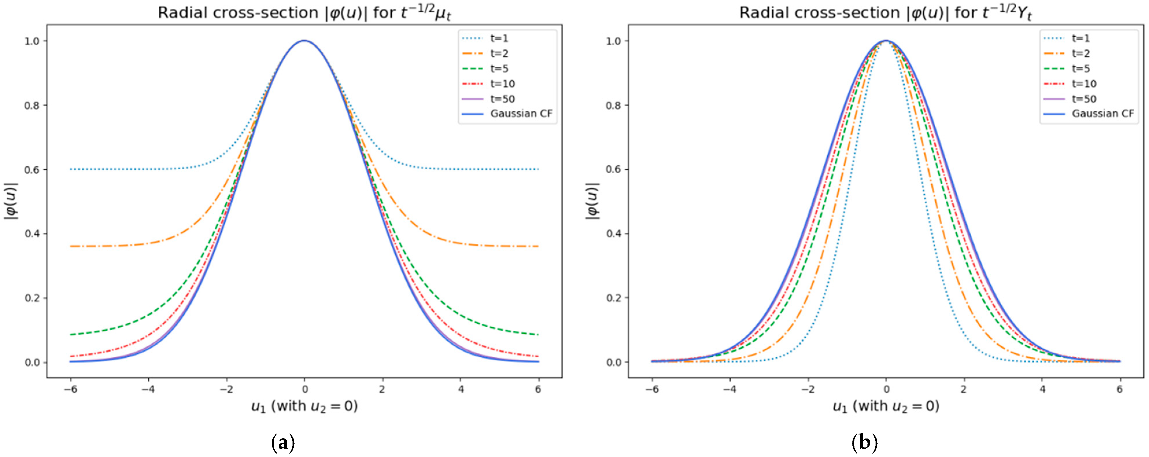
As an illustration, Figure 4 shows the moduli of the CFs for the scaled series ${\mathit{M}}_{\mathit{t};\mathit{\alpha }}$ and ${\mathit{U}}_{\mathit{t};\mathit{\alpha }}$, where several representative values of $\alpha$ are chosen. It should be noted that for $0<\alpha <1$, the normalization is too weak to stabilize the growth of the non-stationary components, and both scaled processes asymptotically have infinite mean and variance. Therefore, this regime does not admit a meaningful asymptotic interpretation and is not considered. The remaining cases mentioned in Theorem 5 can be interpreted as follows:

Figure 4. Moduli of CFs for the bivariate RVs ${\mathit{M}}_{\mathit{t};\mathit{\alpha }}$ (a) and ${\mathit{U}}_{\mathit{t};\mathit{\alpha }}$ (b), with different values of $\alpha$ and $t=50$ (Parameters values are the same as in Figure 3).

• When $1\le \alpha <3/2$, both series ${\mathit{M}}_{\mathit{t};\mathit{\alpha }}$ and ${\mathit{Y}}_{\mathit{t};\mathit{\alpha }}$ have an approximately bivariate Gaussian distribution, with the mean converging to zero, while their variance–covariance matrices diverge.
• When $\alpha >3/2$, both series converge (in distribution) to the zero-vector $\mathbf{0}:={\left(\mathrm{0,0}\right)}^{\top }.$ Hence, according to the well-known facts (see, e.g., Billingsley [20]), the convergence in probability also holds, i.e., ${\mathit{M}}_{\mathit{t};\mathit{\alpha }}\stackrel{P}{⟶}\mathbf{0}, {\mathit{U}}_{\mathit{t};\mathit{\alpha }}\stackrel{P}{⟶}\mathbf{0}, t\to +\infty$.
• The case $\alpha =3/2$ is of special interest, because the asymptotic relations in Equation (23) then become:

$$t^{-3/2}\sum _{j=1}^t{\mathit{\mu }}_{\mathit{j}}\stackrel{d}{⟶}\mathcal{N}\left(0,{\displaystyle \frac{p_c}{3}}\Sigma \right), t^{-3/2}\sum _{j=1}^t{\mathit{Y}}_{\mathit{j}}\stackrel{d}{⟶}\mathcal{N}\left(0,{\displaystyle \frac{p_c}{3}}\Sigma \right), t\to +\mathrm{\infty }.$$

(25)

Note that these convergences, compared to those given by Equation (20), have smaller variances, which is useful in the practical application of the 2D-GSB process.

4. Parameters Estimation

This section addresses the estimation of the unknown parameters of the 2D-GSB process, including the critical threshold $c$ (or equivalently the regime probability $p_c$), the mean vector ${\mathit{\mu }}_{\mathbf{0}}={\left(m_1,m_2\right)}^{\mathrm{\top }}$, and the elements of the covariance matrix (${\sigma }_1^2, {\sigma }_2^2, \rho$). To this end, note that although the original 2D-GSB components $\left({\mathit{Y}}_{\mathit{t}}\right)$ and $\left({\mathit{\mu }}_{\mathit{t}}\right)$ are non-stationary, their asymptotic results are derived under appropriate scaling, as stated in Theorems 4 and 5. Thus, the estimation of the mean structure relies on these scaling results and on the observed series $\left({\mathit{Y}}_{\mathit{t}}\right)$. In contrast, the estimation of the remaining parameters is primarily based on the stationary increment process $\left(X_t\right)$, whose stochastic properties are formally established by Theorems 2 and 3. Note the specific mixture-based structure of $\left({\mathit{X}}_t\right)$ requires additional considerations and a careful assessment of estimator performance. At the beginning, the method of moments (MoM) is applied first, followed by the empirical characteristic function (ECF) approach. Under suitable regularity conditions, the asymptotic properties of both estimators are established, and their finite-sample performance is also compared.

4.1. Moment-Based Estimators

Let $\left({\mathit{X}}_t\right)$, $t=\mathrm{0,1},\dots ,n$ be some realization of the increments of the 2D-GSB process, where ${\mathit{X}}_0={\left(\mathrm{0,0}\right)}^{\mathrm{\top }}$. According to Theorem 2, that is, Equation (13), for the covariance of the series $\left({\mathit{X}}_t\right)$ is valid

$${\Gamma }_X\left(0\right)=\mathrm{C}\mathrm{o}\mathrm{v}\left({\mathit{X}}_{\mathit{t}},{\mathit{X}}_{\mathit{t}}\right)=(2-p_{\mathrm{c}})·\Sigma , {\Gamma }_X\left(1\right)=\mathrm{C}\mathrm{o}\mathrm{v}\left({\mathit{X}}_{\mathit{t}},{\mathit{X}}_{\mathit{t}-\mathbf{1}}\right)=(p_{\mathrm{c}}-1)·\Sigma ,$$

from where it follows:

$${\Gamma }_X\left(1\right)={\displaystyle \frac{p_{\mathrm{c}}-1}{2-p_{\mathrm{c}}}}·{\Gamma }_X\left(0\right).$$

According to this and using the sample covariance matrices

$${\widehat{\Gamma }}_X\left(0\right)={\displaystyle \frac{1}{n}}\sum _{t=1}^n{\mathit{X}}_t{\mathit{X}}_t^{\mathrm{\top }}, {\widehat{\Gamma }}_X\left(1\right)={\displaystyle \frac{1}{n-1}}\sum _{t=2}^n{\mathit{X}}_t{\mathit{X}}_{t-1}^{\mathrm{\top }}$$

the following estimator of the proportion $r=(p_{\mathrm{c}}-1)/(2-p_{\mathrm{c}})$ can be calculated

$$\widehat{r}={\displaystyle \frac{\mathrm{t}\mathrm{r} {\widehat{\Gamma }}_X\left(1\right)}{\mathrm{t}\mathrm{r} {\widehat{\Gamma }}_X\left(0\right)}},$$

(26)

where $\mathrm{t}\mathrm{r} {\widehat{\Gamma }}_X\left(0\right)$ and $\mathrm{t}\mathrm{r} {\widehat{\Gamma }}_X\left(1\right)$ are the traces of the given matrices. Then, for the estimator of the parameter $p_{\mathrm{c}}$ one obtains:

$${\widehat{p}}_c={\displaystyle \frac{1+2\widehat{r}}{1+\widehat{r}}}.$$

(27)

Based on the estimator ${\widehat{p}}_c$, the corresponding estimator of the critical value $c=\widehat{c}$ can be determined as a solution to the equation:

$$P\left\{{‖{\mathit{\epsilon }}_{\mathit{t}}‖}^2>c\right\}={\widehat{p}}_c.$$

According to Equations (14) and (26), it can be easily seen that ${\widehat{p}}_c$ and $\widehat{c}$ are the appropriate estimators if the following inequalities hold:

$$0<{\widehat{p}}_c<1⟺-0.5<\widehat{r}<0.$$

Note that these conditions are equivalent to those for a one-dimensional GSB process (see, e.g., Jovanović et al. [12]). On the other hand, using the estimator ${\widehat{p}}_c$, the covariance matrix of the 2D-GSB process can be estimated from the equation:

$$\widehat{\Sigma }={\displaystyle \frac{1}{2-{\widehat{p}}_c}}{\widehat{\Gamma }}_X\left(0\right).$$

(28)

For the estimators ${\widehat{p}}_c$ and $\widehat{\Sigma }$, given by Equations (27) and (28), respectively, we say that they represent MoM estimators for the parameter $p_c$ and covariance matrix $\Sigma$. At the same time, their consistency and asymptotic normality can be proven. To this end, we first prove the strict law of large numbers (SLLN) and almost surely (a.s.) consistency for the so-called moment-vectors, used in the construction of the MoM estimators.

Theorem 6.

Let $\left({\mathit{X}}_{\mathit{t}}\right)$ be the increment series of the 2D-GSB process, defined by Equations (11) and (12). Then, for the vectors ${\mathit{Z}}_{\mathit{t}}≔vec({\mathit{X}}_{\mathit{t}}{\mathit{X}}_{\mathit{t}}^{\mathit{\top }},{\mathit{X}}_{\mathit{t}}{\mathit{X}}_{\mathit{t}-1}^{\top })\in {\mathbb{R}}^8$ the following statements hold:

(i) 

$\mathbb{E}{‖{\mathit{Z}}_{\mathit{t}}‖}^2<+\mathrm{\infty }$, for any $t=\mathrm{1,2},\dots ,n$.

(ii) 

The series $\left({\mathit{Z}}_{\mathit{t}}\right)$ is 2-dependent, i.e., each ${\mathit{Z}}_{\mathit{t}}$ and ${\mathit{Z}}_{\mathit{s}}$ are independent when $\left|t-s\right|>2$.

(iii) 

The moment-vector ${\mathit{V}}_{\mathit{n}}≔n^{-1}{\sum }_{t=1}^n{\mathit{Z}}_{\mathit{t}}$ converges almost surely to $\mathbb{E}\left({\mathit{Z}}_{\mathbf{1}}\right)$, i.e.,

$${\displaystyle \frac{1}{n}}\sum _{t=1}^n{\mathit{Z}}_{\mathit{t}}\stackrel{a.s.}{⟶}\mathbb{E}\left({\mathit{Z}}_1\right), n\to +\mathrm{\infty }.$$

(29)

(iv) 

The series $\left({\mathit{V}}_{\mathit{n}}\right)$ is asymptotically normal, i.e.,

$$\sqrt{n}\left({\mathit{V}}_{\mathit{n}}-\mathbb{E}\left({\mathit{Z}}_{\mathbf{1}}\right)\right)\stackrel{d}{⟶}\mathcal{N}\left(\mathbf{0},\Omega \right), n\to +\mathrm{\infty },$$

(30)

where $\Omega ≔{\sum }_{h=-2}^2\mathrm{Cov}\left({\mathit{Z}}_{\mathit{t}},{\mathit{Z}}_{\mathit{t}+\mathit{h}}\right)=\mathrm{Var}\left({\mathit{Z}}_{\mathit{t}}\right)+2(\mathrm{Cov}\left({\mathit{Z}}_{\mathit{t}},{\mathit{Z}}_{\mathit{t}+1}\right)+\mathrm{Cov}\left({\mathit{Z}}_{\mathit{t}},{\mathit{Z}}_{\mathit{t}+2}\right))$.

Proof. 

(i) Since the components of the vector ${\mathit{Z}}_{\mathit{t}}$ are the products of the components of the vectors ${\mathit{X}}_{\mathit{t}}$ and ${\mathit{X}}_{\mathit{t}-\mathbf{1}}$, it is sufficient to show that the fourth moments of the increments are finite, i.e., $\mathbb{E}{‖{\mathit{X}}_{\mathit{t}}‖}^4<+\infty$, when $t=\mathrm{1,2},\dots ,n.$ For this purpose, we use Jensen’s inequality (see, e.g., [21])

$${\left(a+b\right)}^p\le 2^{p-1}\left(a^p+b^p\right),$$

which holds for any $a,b\ge 0$ and $p\ge 1.$ By putting $p=4$ and applying this inequality on Equation (11), one obtains:

$$\left|\right|{\mathit{X}}_{\mathit{t}}{\left|\right|}^4\le 8\left(\left|\right|{\mathbf{\epsilon }}_{\mathit{t}}|{|}^4+|\left|r_{t-1}{\mathbf{\epsilon }}_{\mathit{t}-\mathbf{1}}\right|{|}^4\right)=8\left(\left|\right|{\mathbf{\epsilon }}_{\mathit{t}}|{|}^4+r_{t-1}|\left|{\mathbf{\epsilon }}_{\mathit{t}-\mathbf{1}}\right|{|}^4\right).$$

Taking the expectation and using the inequality $r_{t-1}\le 1$, as well as the stationarity of the innovations $({\mathbf{\epsilon }}_{\mathit{t}}$), it follows from here that:

$$\mathbb{E}\left|\right|{\mathit{X}}_{\mathit{t}}{\left|\right|}^4\le 8\left(\mathbb{E}\left|\right|{\mathit{\epsilon }}_{\mathit{t}}|{|}^4+\mathbb{E}|\left|{\mathit{\epsilon }}_{\mathit{t}-1}\right|{|}^4\right)=16\hspace{0.17em}\mathbb{E}\left|\right|{\mathit{\epsilon }}_{\mathit{t}}|{|}^4.$$

In doing so, the series ${\mathbf{\epsilon }}_{\mathit{t}}={({\epsilon }_t^{\left(1\right)},{\epsilon }_t^{\left(2\right)})}^T\sim \mathcal{N}\left(\mathbf{0},\Sigma \right)$ have the finite moments of all orders, in particular:

$$\mathbb{E}\left|\right|{\mathit{\epsilon }}_{\mathit{t}}|{|}^4=\mathbb{E}\left({\left({\epsilon }_t^{\left(1\right)}\right)}^4+2{\left({\epsilon }_t^{\left(1\right)}\right)}^2{\left({\epsilon }_t^{\left(2\right)}\right)}^2+{\left({\epsilon }_t^{\left(2\right)}\right)}^4\right)=3{\sigma }_1^4+2{\sigma }_1^2{\sigma }_2^2\left(1+2{\rho }^2\right)+3{\sigma }_2^4.$$

Thus, $\mathbb{E}\left|\right|{\mathit{\epsilon }}_{\mathit{t}}|{|}^4<+\mathrm{\infty }$ holds, and therefore $\mathbb{E}\left|\right|{\mathit{X}}_{\mathit{t}}|{|}^4<+\mathrm{\infty }$.

(ii) By the definition of the increment $\left({\mathit{X}}_{\mathit{t}}\right)$, they depend (only) on the RVs ${\mathbf{\epsilon }}_{\mathit{t}}$ and ${\mathbf{\epsilon }}_{\mathit{t}-1}$, for each $t=\mathrm{1,2}\dots$ Since $\left({\mathbf{\epsilon }}_{\mathit{t}}\right)$ is an IID series, it follows that $\left({\mathit{X}}_{\mathit{t}}\right)$ is a 1-dependent time series. Similarly, the components ${\mathit{X}}_{\mathit{t}}{\mathit{X}}_{\mathit{t}-\mathbf{1}}^{\mathbf{\top }}$ depend on ${\mathbf{\epsilon }}_{\mathit{t}},{\mathbf{\epsilon }}_{\mathit{t}-1},{\mathbf{\epsilon }}_{\mathit{t}-2}$, while ${\mathit{X}}_{\mathit{t}}{\mathit{X}}_{\mathit{t}}^{\mathbf{\top }}$ depends on ${\mathbf{\epsilon }}_{\mathit{t}},{\mathbf{\epsilon }}_{\mathit{t}-\mathbf{1}}$. Therefore, ${\mathit{Z}}_{\mathit{t}}$ depends at most on the set of RVs $\{{\mathbf{\epsilon }}_{\mathit{t}-\mathbf{2}},{\mathbf{\epsilon }}_{\mathit{t}-\mathbf{1}},{\mathbf{\epsilon }}_{\mathit{t}}\}$, so the vector series $\left({\mathit{Z}}_{\mathit{t}}\right)$ is indeed 2-dependent.

(iii) Since the series $\left({\mathit{Z}}_{\mathit{t}}\right)$ is 2-dependent, we divide the indices into following three subsets (with remainder modulo 3):

$$A_0=\{1,4,7,\dots \}, A_1=\{2,5,8,\dots \}, A_2=\{3,6,9,\dots \}.$$

Thus, for a fixed $j\in \{0,1,2\}$, the elements of sets $S_j≔\{{\mathit{Z}}_{\mathit{t}} | t\in A_j\}$ are independent, and according to (i), they have a common finite moment $E{‖{\mathit{Z}}_{\mathit{t}}‖}^2$. By applying Kolmogorov’s SLLN for an IID series (see, e.g., [22]), we get

$${\displaystyle \frac{1}{\left|A_j\left(n\right)\right|}}\sum _{t\in A_j,\hspace{0.17em}t\le n}{\mathit{Z}}_{\mathit{t}}\stackrel{\mathrm{a}\mathrm{s}}{⟶}\mathbb{E}\left({\mathit{Z}}_{\mathbf{1}}\right), n\to +\infty ,$$

where $\left|A_j\left(n\right)\right|$ is the number of elements of the set $A_j$ that are less or equal to $n$. According to this, it follows that $\left|A_j\left(n\right)\right|/n\to 1/3,$ when $n\to +\infty ,$ which implies:

$${\displaystyle \frac{1}{n}}\sum _{t=1}^n{\mathit{Z}}_{\mathit{t}}=\sum _{j=0}^2{\displaystyle \frac{\left|A_j\left(n\right)\right|}{n}}\cdot {\displaystyle \frac{1}{\left|A_j\left(n\right)\right|}}\sum _{t\in A_j,\hspace{0.17em}t\le n}{\mathit{Z}}_{\mathit{t}}\stackrel{\mathrm{a}.\mathrm{s}.}{⟶}\sum _{j=0}^2{\displaystyle \frac{1}{3}}\mathbb{E}\left({\mathit{Z}}_{\mathbf{1}}\right)=\mathbb{E}\left({\mathit{Z}}_{\mathbf{1}}\right), n\to +\infty .$$

This proves the convergence in Equation (29).

(iv) Let $\mathbf{a}\in {\mathbb{R}}^2$ be an arbitrary fixed vector. According to the above, $U_t≔{\mathit{a}}^{\mathrm{\top }}{\mathit{Z}}_{\mathit{t}}$ is a stationary and 2-dependent series of scalar RVs, with a finite second moment:

$$\mathbb{E}\left(U_t^2\right)\le \left|\right|\mathbf{a}\left|{|}^2\mathbb{E}\right|{|\mathit{Z}}_{\mathit{t}}|{|}^2<+\mathrm{\infty }.$$

Hence, by applying the Hoeffding–Robbins CLT for $m$-dependent scalar series [23], one obtains

$$\sqrt{n}\left({\overline{U}}_n-\mathbb{E}\left(U_1\right)\right)\stackrel{d}{⟶}\mathcal{N}\left(\mathbf{0},{\sigma }_{\mathrm{a}}^2\right), n\to +\mathrm{\infty },$$

where ${\overline{U}}_n=n^{-1}\sum _{k=1}^n{U}_k$ and

$${\sigma }_{\mathrm{a}}^2=\sum _{h=-m}^m\mathrm{Cov}\left(U_t,U_{t+h}\right)={\mathbf{a}}^{\mathrm{\top }}\left(\sum _{h=-m}^m\mathrm{C}\mathrm{o}\mathrm{v}\left({\mathit{Z}}_{\mathit{t}},{\mathit{Z}}_{\mathit{t}+\mathit{h}}\right)\right)\mathbf{a}={\mathbf{a}}^{\mathrm{\top }}\Omega \mathbf{a},$$

with $m=2$. Since the above is true for every $\mathbf{a}\in {\mathbb{R}}^2$, the Cramér–Wold decomposition [24] implies multivariate normality as given by Equation (30). □

As a consequence of the previous theorem, it follows:

Corollary 1.

Let ${\theta }_0=\left(p_0,{\Sigma }_0\right)$ be the true value of the unknown parameter vector $\theta =\left(p_c,\Sigma \right)$ of the 2D-GSB process, where $p_0\in \left(\mathrm{0,1}\right)$ and ${\Sigma }_0$ is a $2\times 2$ positive-definite matrix. Then, the estimator ${\widehat{\theta }}_n=\left({\widehat{p}}_c,\widehat{\Sigma }\right),$ defined by Equations (26)–(28), is strongly consistent for ${\theta }_0$, i.e.,

$${\widehat{\theta }}_n\stackrel{as}{⟶}{\theta }_0, n\to +\infty .$$

(31)

In addition, ${\widehat{\theta }}_n$ is an asymptotically normal estimator for ${\theta }_0$, i.e.,

$$\sqrt{n}\left({\widehat{\theta }}_n-{\theta }_0\right)\stackrel{d}{⟶}\mathcal{N}\left(0,V\right), n\to +\infty ,$$

(32)

where $V=D^{\top }\Omega \hspace{0.17em}D,$ $D={\left.\mathsf{\partial }m\left(\theta \right)/\mathsf{\partial }{\theta }^{\top }\right|}_{\theta ={\theta }_0},$ $m\left(\theta \right)={\left(f\left(r\left(\theta \right)\right),g\left(\theta \right)\right)}^{\top },$ $f\left(r\right)=\left(2r+1\right)/\left(1+r\right),$ $r\left(\theta \right)=tr \Gamma \left(1,\theta \right)/tr \Gamma \left(0,\theta \right),$ $g\left(\theta \right)=\Gamma \left(0,\theta \right)/\left(2-f\left(r\left(\theta \right)\right)\right),$ $\Gamma \left(h;\theta \right)=\mathrm{C}\mathrm{o}{\mathrm{v}}_{\mathsf{\theta }}\left({\mathit{X}}_{\mathit{t}},{\mathit{X}}_{\mathit{t}-\mathit{h}}\right)$.

Proof. 

It is obvious that $\theta \mapsto m\left(\theta \right)$ is an injective continuous mapping, well-defined in some neighborhood of the true parameters ${\theta }_0$. Thus, according to the continuity of almost-sure convergence, as well as the convergence in distribution (see, e.g., Serfling [25] (pp. 24)), the statement of the theorem immediately follows. □

Remark 6.

According to Corollary 1 and Equations (26)–(28), it is valid that ${\widehat{p}}_c=f\left(\widehat{r}\right)$. In addition, the vectors $(A_n,B_n{)}^{\mathrm{\top }}={(\mathrm{tr}{\widehat{\Gamma }}_X\left(0\right),\mathrm{tr}{\widehat{\Gamma }}_X\left(1\right))}^{\mathrm{\top }}$ are linear functionals of the moment-vector ${\mathit{V}}_{\mathit{n}}$, defined in Theorem 5, which implies

$$\sqrt{n}\left(\begin{array}{c}{A}_n-A_0\\ B_n-B_0\end{array}\right)\hspace{0.25em}\stackrel{d}{\to }\hspace{0.25em}\mathcal{N} \left(0,{\Sigma }_{AB}\right),$$

where $A_0=tr{\Gamma }_X\left(0\right)$, $B_0=tr{\Gamma }_X\left(1\right)$, and

$${\Sigma }_{AB}=\underset{n\to \mathrm{\infty }}{\mathrm{l}\mathrm{i}\mathrm{m}} \mathrm{C}\mathrm{o}\mathrm{v}\left(\sqrt{n}\left(\begin{array}{c}{A}_n-A_0\\ B_n-B_0\end{array}\right)\right)=\underset{n\to \mathrm{\infty }}{\mathrm{l}\mathrm{i}\mathrm{m}}\left(\begin{array}{cc}\mathrm{V}\mathrm{a}\mathrm{r}(\sqrt{n} A_n)& \mathrm{C}\mathrm{o}\mathrm{v}(\sqrt{n} A_n,\sqrt{n} B_n)\\ \mathrm{C}\mathrm{o}\mathrm{v}(\sqrt{n} A_n,\sqrt{n} B_n)& \mathrm{V}\mathrm{a}\mathrm{r}(\sqrt{n} B_n)\end{array}\right)$$

denotes the asymptotic covariance matrix of the vector $(A_n,B_n{)}^{\top }$, which is obtained as a linear transformation of the limiting covariance matrix $\Omega ,$ given by Equation (30). Thus, after some computation, for the asymptotic variance of ${\widehat{p}}_c$ one obtains

$$V_1=f^{\prime }{\left(r_0\right)}^2\cdot \mathrm{Var}\left(\sqrt{n}\widehat{r}\right)={\displaystyle \frac{B_0^2 \mathrm{V}\mathrm{a}\mathrm{r}\left(A_n\right)-2A_0{B}_0 \mathrm{C}\mathrm{o}\mathrm{v}\left(A_n,B_n\right)+A_0^2 \mathrm{V}\mathrm{a}\mathrm{r}\left(B_n\right)}{A_0^4\left(1+r_0{)}^4\right.}},$$

where $r_0$ denotes the true value of the ratio $r\left({\theta }_0\right).$ This shows that the asymptotic efficiency of the estimator ${\widehat{p}}_c$ is fully determined by the second-order dependence structure of the increment process $\left({\mathit{X}}_{\mathit{t}}\right)$, summarized through the scalar statistic $r$. Moreover, it allows for a simplified variance estimation in practical applications, without requiring the full covariance matrix $\Omega$. Finally, it should be noted that similar considerations are also possible for the estimator $\hat{\Sigma }$, defined by Equation (28).

4.2. ECF Estimators

In this section, the unknown parameters of the 2D-GSB process are estimated using the ECF method, which was first rigorously developed in the pioneering works of Knight and Yu [26] and Yu [27]. Subsequent extensions of CF-based estimators have been discussed by Kotchoni [28], Meintanis et al. [29,30] and other authors. Following these contributions, an ECF procedure similar to those in Stojanović et al. [13] and Ljajko et al. [15] is employed here. The key idea underlying the ECF method is the bijective correspondence between CFs and their corresponding CDFs, implying that ECF retains all distributional information contained in the sample. Moreover, theoretical CFs are uniformly bounded, which contributes to the numerical stability of the resulting estimators. To this end, a general expression for the $r$-th order CFs ($r\ge 1$) of the increment series (${\mathit{X}}_{\mathit{t}}$) of the 2D-GSB process is first presented:

Theorem 7.

Let the bivariate series of increments $\left({\mathit{X}}_{\mathit{t}}\right)$ be defined by Equations (11) and (12), and $\theta =\left(p_c,\Sigma \right)$ is a vector of unknown parameters. Then, for any block length $\mathsf{\ell }\ge 1$ and any vector $\mathit{u}=(u_1,\dots ,u_{\mathsf{\ell }})\in ({\mathbb{R}}^2{)}^{\mathsf{\ell }}$ the $\mathsf{\ell }$-dimensional characteristic function

$${\phi }_X^{\left(\mathsf{\ell }\right)}\left(\mathit{u};\theta \right)=\mathbb{E}\mathit{exp}\left(i\sum _{k=1}^{\mathsf{\ell }}{u}_k^{\top }{\mathit{X}}_{\mathit{t}+\mathit{k}-\mathbf{1}}\right)$$

(33)

admits the explicit representation

$${\phi }_X^{\left(\mathsf{\ell }\right)}\left(\mathbf{u};\theta \right)=\exp \left(-{\displaystyle \frac{1}{2}}{‖u_{\mathsf{\ell }}‖}_{\Sigma }^2\right)\prod _{k=0}^{\mathsf{\ell }-1}\left[p_c \exp \left(-{\displaystyle \frac{1}{2}}{‖u_k‖}_{\Sigma }^2\right)+(1-p_c) \exp \left(-{‖u_k-u_{k+1}‖}_{\Sigma }^2\right)\right]$$

(34)

where $u_0={\mathbf{0}}_{\mathbf{2}\times \mathbf{1}}$, $p_c=P\left\{{‖{\mathit{\epsilon }}_{\mathit{t}}‖}^2>c\right\}$, and ${‖u‖}_{\Sigma }^2:=u^{\mathrm{\top }}\Sigma u$, when $u\in {\mathbb{R}}^2$.

Proof. 

First, let us note that, according to Equation (18), the statement of the theorem is valid for the case when $\mathsf{\ell }=1$ and $u_1=\mathbf{u}$. Now, assume that $\mathsf{\ell }>1$ and denote:

$$\begin{gathered} \mathcal{L}\left(\mathbf{u};\theta \right)≔\exp \left(\mathrm{i}\sum _{k=1}^{\mathsf{\ell }}{u}_k^{\mathrm{\top }}{\mathit{X}}_{\mathit{t}+\mathit{k}-\mathbf{1}}\right)=\exp \left[\mathrm{i}\sum _{k=1}^{\mathsf{\ell }}{u}_k^{\mathrm{\top }}\left({\mathit{\epsilon }}_{\mathit{t}+\mathit{k}-\mathbf{1}}-r_{t+k-2}{\mathit{\epsilon }}_{\mathit{t}+\mathit{k}-\mathbf{2}}\right)\right] \\ =\exp \left[\mathrm{i}\left(u_{\mathsf{\ell }}^{\mathrm{\top }}{\mathit{\epsilon }}_{\mathit{t}+\mathsf{\ell }-\mathbf{1}}+\sum _{k=0}^{\mathsf{\ell }-1}\left(u_k^{\mathrm{\top }}-r_{t+k-1}{u}_{k+1}^{\mathrm{\top }}\right){\mathit{\epsilon }}_{\mathit{t}+\mathit{k}-\mathbf{1}}\right)\right]. \end{gathered}$$

According to this and Equation (33), the $\mathsf{\ell }$-dimensional CF of the series $\left({\mathit{X}}_{\mathit{t}}\right)$ is obtained as ${\phi }_X^{\left(\mathsf{\ell }\right)}(\mathbf{u};\theta ):=E\left[\mathcal{L}\left(\mathbf{u};\theta \right)\right]$, from which, after some elementary calculations, Equation (34) is easily shown. □

Next, let us denote by $\left\{{\mathit{X}}_1,\dots ,{\mathit{X}}_{\mathit{n}}\right\}$ some realization of length $n\in \mathbb{N}$ of the increments $\left({\mathit{X}}_{\mathit{t}}\right)$, as well as their corresponding $\mathsf{\ell }$-dimensional ECF

$${\widehat{\phi }}_n^{(\mathsf{\ell })}\left(\mathbf{u}\right)\mathrm{ }≔{\displaystyle \frac{1}{n-\mathsf{\ell }+1}}\sum _{t=1}^{n-\mathsf{\ell }+1}\exp \left(\mathrm{i}{\mathbf{u}}^{\mathrm{\top }}{\mathit{X}}_t^{\left(\mathsf{\ell }\right)}\mathrm{ }\right),$$

(35)

where ${\mathit{X}}_t^{\left(\mathsf{\ell }\right)}≔({\mathit{X}}_{\mathit{t}},\dots ,{\mathit{X}}_{\mathit{t}+\mathcal{l}-\mathbf{1}})$ is the overlapping block of length $\mathsf{\ell }\ge 1.$ The basic principle of the ECF method is to minimize the “distance” between the theoretical CF and its corresponding ECF, where ECF estimators are obtained by minimizing the objective function

$$Q_n^{\left(\mathsf{\ell }\right)}\left(\theta \right)≔{\int }_{{\mathbb{R}}^{2\mathsf{\ell }}}g\left(\mathbf{u}\right){\left|{\widehat{\phi }}_n^{(\mathsf{\ell })}\left(\mathbf{u}\right)-{\phi }_X^{\left(\mathsf{\ell }\right)}\left(\mathbf{u};\theta \right)\right|}^2\mathbf{d}\mathbf{u}$$

(36)

with respect to the parameters $\theta =\left(p_c,\Sigma \right)$. Here, we denote it as $\mathbf{d}\mathbf{u}≔\mathrm{d}{u}_1\cdots \mathrm{d}{u}_{\mathsf{\ell }}$, and $g:{\mathbb{R}}^{2\mathsf{\ell }}\to {\mathbb{R}}^{+}$ is some weight function. Therefore, the ECF estimates are solutions to the following minimization equation:

$${\widehat{\theta }}_n^{\left(\mathsf{\ell }\right)}=\arg \underset{\theta \in \mathsf{\Theta }}{\min }{Q}_n^{\left(\mathsf{\ell }\right)}\left(\theta \right),$$

(37)

where $\mathsf{\Theta }=\left(\mathrm{0,1}\right)\times {\left(0,+\mathrm{\infty }\right)}^3$ is a non-trivial parameter space. Using some general results of the ECF asymptotic theory, the strong consistency and asymptotic normality (AN) of the ECF estimators, under certain regulatory conditions, can be proven as follows:

Theorem 8.

Let ${\theta }_0$ be the true value of the parameter $\theta$, and for arbitrary $n=1, 2,\dots ,$ let ${\hat{\theta }}_n^{\left(\mathsf{\ell }\right)}$be the solutions of Equation (37). In addition, assume that the following regularity conditions are satisfied:

• (R₁) The weight function $g\left(\mathbf{u}\right)$ is real-valued, nonnegative and integrable, with

  $${\int }_{{\mathbb{R}}^{2\mathsf{\ell }}}{‖\mathbf{u}‖}^{2}g\left(\mathbf{u}\right) \mathrm{d}\mathbf{u}<+\mathrm{\infty }.$$
• (R₂) The parameter $\theta$ is identifiable from the ℓ-dimensional CF, given by Equations (33) and (34), i.e., from the equality ${\phi }_X^{\left(\mathsf{\ell }\right)}\left(\mathbf{u};{\theta }_1\right)={\phi }_X^{\left(\mathsf{\ell }\right)}\left(\mathbf{u};{\theta }_2\right),$ for almost all $\mathbf{u}\in {\mathbb{R}}^{2\mathsf{\ell }},$ it follows ${\theta }_1={\theta }_2,$ for any ${\theta }_1,{\theta }_2\in \mathsf{\Theta }.$
• (R₃) There exists the compact set ${\Theta }^{\prime }=\left[\mathrm{0,1}\right]\times {\left[0,M\right]}^3\subset \overline{\Theta }$, where M is sufficiently large so that  ${\theta }_0,{\widehat{\theta }}_n^{\left(\mathsf{\ell }\right)}\in int {\Theta }^{\prime }$, for any $n\ge n_0>0.$
• (R₄) The function ${\phi }_X^{\left(\mathsf{\ell }\right)}(\mathit{u};\theta )$ is twice continuously differentiable with respect to $\theta$, uniformly in $\mathit{u}\in {\mathbb{R}}^{2\mathsf{\ell }}.$
• (R₅) ${\left.{\mathit{\nabla }}_{\theta }^2{Q}_n^{\left(\mathsf{\ell }\right)}\left(\theta \right)\right|}_{\theta ={\theta }_0}$ is a positive definite, regular, non-zero matrix.
• Then, for any $\mathsf{\ell }\ge 2,$ ${\widehat{\theta }}_n^{\left(\mathsf{\ell }\right)}$ is a strictly consistent and asymptotically normal estimator for θ.

Proof. 

First, relabel the ECF and the $\mathsf{\ell }$-blocks, defined by Equation (35), as follows:

$${\widehat{\phi }}_n^{\left(\mathsf{\ell }\right)}\left(\mathbf{u}\right)={\displaystyle \frac{1}{n-\mathsf{\ell }+1}}\sum _{t=1}^{n-\mathsf{\ell }+1}{W}_t\left(\mathbf{u}\right), W_t(\mathbf{u}):=\exp \left(\mathrm{i}\sum _{j=1}^{\mathsf{\ell }}{u}_j^{\mathrm{\top }}{\mathit{X}}_{\mathit{t}+\mathit{j}-\mathbf{1}}\right).$$

By construction of the increment process (${\mathit{X}}_{\mathit{t}})$, for each fixed $\mathbf{u}\in {\mathbb{R}}^{2\mathsf{\ell }}$ the series $\left(W_t\right(\mathbf{u}){)}_{t\ge 1}$ is strictly stationary and $\mathsf{\ell }+1$-dependent. Furthermore, the equality $\left|W_t\left(\mathbf{u}\right)\right|=1$ holds for any $t\ge 1$ and $\mathbf{u}\in {\mathbb{R}}^{2\mathsf{\ell }}$, so that $W_t\left(\mathbf{u}\right)\in L^1$. Hence, by applying the SSLN for $m$-dependent stationary series (see, e.g., [31]), it follows that

$${\widehat{\phi }}_n^{\left(\mathsf{\ell }\right)}\left(\mathbf{u}\right)\hspace{0.25em}\stackrel{a.s.}{\to }\hspace{0.25em}\mathbb{E}\left[W_1\left(\mathbf{u}\right)\right]={\phi }_X^{\left(\mathsf{\ell }\right)}\left(\mathbf{u};{\theta }_0\right),$$

for each fixed $\mathbf{u}\in {\mathbb{R}}^{2\mathsf{\ell }}.$ According to the continuity of the CFs defined in (33) and (34), the pointwise convergence above implies uniform convergence on any compact $C\subset {\mathbb{R}}^{2\mathsf{\ell }},$ i.e.,

$$\underset{\mathbf{u}\in C}{\mathrm{s}\mathrm{u}\mathrm{p}}\left|{\widehat{\phi }}_n^{\left(\mathsf{\ell }\right)}\left(\mathbf{u}\right)-{\phi }_X^{\left(\mathsf{\ell }\right)}\left(\mathbf{u};{\theta }_0\right)\right|\stackrel{a.s.}{\to } 0, n\to +\infty .$$

(38)

Further, if we define the function

$$Q_0^{\left(\mathsf{\ell }\right)}\left(\theta \right):={\int }_{{\mathbb{R}}^{2\mathsf{\ell }}}g\left(\mathbf{u}\right){\left|{\phi }_X^{\left(\mathsf{\ell }\right)}\left(\mathbf{u};{\theta }_0\right)-{\phi }_X^{\left(\mathsf{\ell }\right)}\left(\mathbf{u};\theta \right)\right|}^2\mathbf{d}\mathbf{u}\ge 0,$$

then, according to condition (R₁), it is well defined and continuous on the compact ${\mathsf{\Theta }}^{\prime }$. Additionally, from the equality $Q_0^{\left(\mathsf{\ell }\right)}\left(\theta \right)=0$ and condition (R₂) it follows that $\theta ={\theta }_0$; that is, $Q_0^{\left(\mathsf{\ell }\right)}\left(\theta \right)$ has a unique minimum at the point ${\theta }_0$.

On the other hand, since both the empirical and theoretical CFs are uniformly bounded by one, using a similar procedure as in Knight and Yu [26], one obtains:

$$\begin{gathered} \left|Q_n^{\left(\mathsf{\ell }\right)}\left(\theta \right)-Q_0^{\left(\mathsf{\ell }\right)}\left(\theta \right)\right|={\int }_{{\mathbb{R}}^{2\mathsf{\ell }}}g\left(\mathbf{u}\right)\left({\left|{\widehat{\phi }}_n^{\left(\mathsf{\ell }\right)}\left(\mathbf{u}\right)-{\phi }_X^{\left(\mathsf{\ell }\right)}\left(\mathbf{u};\theta \right)\right|}^2-{\left|{\phi }_X^{\left(\mathsf{\ell }\right)}\left(\mathbf{u};{\theta }_0\right)-{\phi }_X^{\left(\mathsf{\ell }\right)}\left(\mathbf{u};\theta \right)\right|}^2\right)\mathbf{d}\mathbf{u} \\ \le {\int }_{{\mathbb{R}}^{2\mathsf{\ell }}}g\left(\mathbf{u}\right)\left|{\widehat{\phi }}_n^{\left(\mathsf{\ell }\right)}\left(\mathbf{u}\right)-{\phi }_X^{\left(\mathsf{\ell }\right)}(\mathbf{u};{\theta }_0)\right|\left(\left|{\widehat{\phi }}_n^{\left(\mathsf{\ell }\right)}\left(\mathbf{u}\right)-{\phi }_X^{\left(\mathsf{\ell }\right)}\left(\mathbf{u};\theta \right)\right|+\left|{\phi }_X^{\left(\mathsf{\ell }\right)}(\mathbf{u};{\theta }_0)-{\phi }_X^{\left(\mathsf{\ell }\right)}(\mathbf{u};\theta )\right|\right)\mathbf{d}\mathbf{u} \\ \le 4{\int }_{{\mathbb{R}}^{2\mathsf{\ell }}}g\left(\mathbf{u}\right)\left|{\widehat{\phi }}_n^{\left(\mathsf{\ell }\right)}\left(\mathbf{u}\right)-{\phi }_X^{\left(\mathsf{\ell }\right)}\left(\mathbf{u};{\theta }_0\right)\right|\mathbf{d}\mathbf{u}. \end{gathered}$$

Hence, convergence (38) and condition (R₃) yield the uniform convergence:

$$\underset{\theta \in {\mathsf{\Theta }}^{\prime }}{\mathrm{s}\mathrm{u}\mathrm{p}}\left|Q_n^{\left(\mathsf{\ell }\right)}\left(\theta \right)-Q_0^{\left(\mathsf{\ell }\right)}\left(\theta \right)\right|\hspace{0.25em}\stackrel{a.s.}{\to }\hspace{0.25em}0, n\to +\infty .$$

Finally, by using Theorem 2.1 in Newey and McFadden [32], we get

$${\widehat{\theta }}_n^{\left(\mathsf{\ell }\right)}\stackrel{a.s.}{\to }{\theta }_0, n\to +\mathrm{\infty },$$

that is, the ECF estimator ${\widehat{\theta }}_n^{\left(\mathsf{\ell }\right)}$ is strictly consistent.

Let us show the AN property of ${\widehat{\theta }}_n^{\left(\mathsf{\ell }\right)}.$ According to condition (R₄), the function $Q_n^{\left(\mathsf{\ell }\right)}\left(\theta \right)$ is twice differentiable near the point $\theta ={\widehat{\theta }}_n^{\left(\mathsf{\ell }\right)}$. Then, using the Taylor expansion of this function, one obtains

$${\nabla }_{\theta }{Q}_n^{\left(\mathsf{\ell }\right)}\left({\widehat{\theta }}_n^{\left(\mathsf{\ell }\right)}\right)={\nabla }_{\theta }{Q}_n^{\left(\mathsf{\ell }\right)}\left({\theta }_0\right)+{\nabla }_{\theta }^2{Q}_n^{\left(\mathsf{\ell }\right)}\left({\overline{\theta }}_n\right)\left({\widehat{\theta }}_n^{\left(\mathsf{\ell }\right)}-{\theta }_0\right),$$

(39)

where ${\overline{\theta }}_T$ is between ${\widehat{\theta }}_n^{\left(\mathsf{\ell }\right)}$ and ${\theta }_0.$ By definition of the ECF estimator ${\widehat{\theta }}_n^{\left(\mathsf{\ell }\right)},$ given by Equation (37), the equality ${\nabla }_{\theta }{Q}_n^{\left(\mathsf{\ell }\right)}\left({\widehat{\theta }}_n^{\left(\mathsf{\ell }\right)}\right)=0$ holds, and from Equation (39) it follows:

$$\sqrt{n}({\widehat{\theta }}_n^{\left(\mathsf{\ell }\right)}-{\theta }_0)=-\left({\nabla }_{\theta }^2{Q}_n^{\left(\mathsf{\ell }\right)}\right({\overline{\theta }}_n){)}^{-1}\sqrt{n} {\nabla }_{\theta }{Q}_n^{\left(\mathsf{\ell }\right)}({\theta }_0).$$

(40)

According to the mentioned properties of the function $Q_n^{\left(\mathsf{\ell }\right)}\left(\theta \right)$, it can be differentiated under the integral sign, i.e.,

$${\nabla }_{\theta }{Q}_n^{\left(\mathsf{\ell }\right)}\left(\theta \right)=-2{\int }_{{\mathbb{R}}^{2\mathsf{\ell }}}g\left(\mathbf{u}\right)\left({\widehat{\phi }}_n^{\left(\mathsf{\ell }\right)}\left(\mathbf{u}\right)-{\phi }_X^{\left(\mathsf{\ell }\right)}\left(\mathbf{u};\theta \right)\right){\mathsf{\nabla }}_{\theta }{\phi }_X^{\left(\mathsf{\ell }\right)}(\mathbf{u};\theta )\mathbf{d}\mathbf{u}$$

(41)

and:

$${\nabla }_{\theta }^2{Q}_n^{\left(\mathsf{\ell }\right)}\left(\theta \right)=2{\int }_{{\mathbb{R}}^{2\mathsf{\ell }}}g\left(\mathbf{u}\right){\nabla }_{\theta }{\phi }_X^{\left(\mathsf{\ell }\right)}(\mathbf{u};\theta ){\nabla }_{\theta }{\phi }_X^{\left(\mathsf{\ell }\right)}(\mathbf{u};\theta {)}^{\mathrm{\top }}\mathbf{d}\mathbf{u}+2{\int }_{{\mathbb{R}}^{2\mathsf{\ell }}}g\left(\mathbf{u}\right)\left({\phi }_X^{\left(\mathsf{\ell }\right)}\left(\mathbf{u};\theta \right)-{\widehat{\phi }}_n^{\left(\mathsf{\ell }\right)}\left(\mathbf{u}\right)\right){\nabla }_{\theta }^2{\phi }_X^{\left(\mathsf{\ell }\right)}\left(\mathbf{u};\theta \right)\mathbf{d}\mathbf{u}.$$

(42)

Thus, by substituting $\theta ={\theta }_0$ and Equation (35) into Equation (41), one obtains

$$\sqrt{n} {\nabla }_{\theta }{Q}_n^{\left(\mathsf{\ell }\right)}({\theta }_0)={\displaystyle \frac{2}{\sqrt{n}}}\sum _{t=1}^n{\psi }_t+o_p(1),$$

where:

$${\psi }_t={\int }_{{\mathbb{R}}^{2\mathsf{\ell }}}g\left(\mathbf{u}\right)\left({\phi }_X^{\left(\mathsf{\ell }\right)}\left(\mathbf{u};{\theta }_0\right)-e^{\mathrm{i}{\mathbf{u}}^{\mathrm{\top }}{X}_t^{\left(\mathsf{\ell }\right)}}\right){\nabla }_{\theta }{\phi }_X^{\left(\mathsf{\ell }\right)}\left(\mathbf{u};{\theta }_0\right)\mathbf{d}\mathbf{u}.$$

In doing so, the series $\left({\psi }_t\right)$ depends on ${\epsilon }_{t-1},\dots ,{\epsilon }_{t+\mathsf{\ell }-1},$ so it is strictly stationary, $\left(\mathsf{\ell }+1\right)$-dependent, with $\mathbb{E}{‖{\psi }_t‖}^2<\mathrm{\infty }.$ Hence, the central limit theorem for a strictly stationary, $\left(\mathsf{\ell }+1\right)$-dependent series with a finite second moment gives

$${\displaystyle \frac{1}{\sqrt{n}}}\sum _{t=1}^n{\psi }_t\stackrel{d}{\to }\mathcal{N}\left(0,D\right),$$

(43)

where $D=\sum _{k=-\mathsf{\ell }}^{\mathsf{\ell }}\mathrm{C}\mathrm{o}\mathrm{v}({\psi }_0,{\psi }_k).$ In addition, the convergence is valid

$${\nabla }_{\theta }^2{Q}_n^{\left(\mathsf{\ell }\right)}\left({\overline{\theta }}_n\right)\stackrel{\mathrm{a}.\mathrm{s}.}{\to }J, n\to +\mathrm{\infty },$$

(44)

where, according to condition (R₅) and Equation (42),

$$J=\mathbb{E}\left({\left.{\nabla }_{\theta }^2{Q}_n^{\left(\mathsf{\ell }\right)}\left(\theta \right)\right|}_{\theta ={\theta }_0}\right)=2{\int }_{{\mathbb{R}}^{2\mathsf{\ell }}}g\left(\mathbf{u}\right){\nabla }_{\theta }{\phi }_X^{\left(\mathsf{\ell }\right)}(\mathbf{u};{\theta }_0){\nabla }_{\theta }{\phi }_X^{\left(\mathsf{\ell }\right)}(\mathbf{u};{\theta }_0{)}^{\mathrm{\top }}\mathbf{d}\mathbf{u}<+\mathrm{\infty }.$$

Thus, Equations (40), (43) and (44) yield

$$\sqrt{n}\left({\widehat{\theta }}_n^{\left(\mathsf{\ell }\right)}-{\theta }_0\right)\stackrel{d}{\to }\mathcal{N}\left(0,J^{-1}D{J}^{-1}\right),$$

that is, the ECF estimator ${\widehat{\theta }}_n^{\left(\mathsf{\ell }\right)}$ is AN for the true parameter ${\theta }_0.$ □

Remark 7.

Note that the asymptotic properties of the ECF estimator for the 2D-GSB model follow the same structural principles as in the one-dimensional case (see, e.g., Stojanović et al. [13]). Thus, the multivariate nature of the increments affects only the analytic form of the CF, while stationarity, short-range dependence and identifiability ensure the validity of the standard ECF asymptotic theory. Moreover, using similar considerations as Yu [27], it can be shown that the above procedure holds if the theoretical CF is of order $\mathsf{\ell }\ge 1$ at least equal to the number of its parameters. For that purpose, $\mathsf{\ell }=2$  is the minimal value ensuring the identifiability of all model parameters. By substituting the value $\mathsf{\ell }=2$ into Equation (34), the explicit form of the CF is as follows:

$$\begin{gathered} {\phi }_X^{\left(2\right)}\left(u_1,u_2\right)=\exp \left(-{\displaystyle \frac{1}{2}} u_2^{\mathrm{\top }}\Sigma u_2\right)\left[p_c^2\mathrm{e}\mathrm{x}\mathrm{p}\left(-{\displaystyle \frac{1}{2}} u_1^{\mathrm{\top }}\Sigma u_1\right)+p_c\left(1-p_c\right)\mathrm{e}\mathrm{x}\mathrm{p}\left(-u_1^{\mathrm{\top }}\Sigma u_1\right) \\ +p_c\left(1-p_c\right)\mathrm{e}\mathrm{x}\mathrm{p}\left(-{\displaystyle \frac{1}{2}} (u_1-u_2{)}^{\mathrm{\top }}\Sigma (u_1-u_2)\right) \\ +{\left(1-p_c\right)}^2\mathrm{e}\mathrm{x}\mathrm{p}\left(-{\displaystyle \frac{1}{2}} (u_1-u_2{)}^{\mathrm{\top }}\Sigma (u_1-u_2)-{\displaystyle \frac{1}{2}} u_1^{\mathrm{\top }}\Sigma u_1\right)\right]. \end{gathered}$$

Thus, we base the estimation procedure on the two-dimensional ECF of the vector series ${\mathit{X}}_t^{\left(2\right)}=(X_t^{\top },X_{t+1}^{\top }{)}^{\top }\in {\mathbb{R}}^4, t=1,\dots ,T-1,$ whose explicit expression for $u=(u_1^{\top },u_2^{\top }{)}^{\top }\in {\mathbb{R}}^4$ is as follows:

$${\widehat{\phi }}_T^{\left(2\right)}\left(u_1,u_2\right)={\displaystyle \frac{1}{n-1}}\sum _{t=1}^{n-1}\mathrm{e}\mathrm{x}\mathrm{p}\left(\mathrm{i}{u}_1^{\mathrm{\top }}{X}_t+i{u}_2^{\mathrm{\top }}{X}_{t+1}\right)={\displaystyle \frac{1}{n-1}}\sum _{t=1}^{n-1}\mathrm{c}\mathrm{o}\mathrm{s}\left(u_1^{\mathrm{\top }}{X}_t+u_2^{\mathrm{\top }}{X}_{t+1}\right)$$

In addition, the choice of the weighting function $g\left(\mathit{u}\right)$ plays a crucial role in the performance of the ECF estimator. In following, we adopt a smooth exponentially decaying weight $g\left(\mathit{u}\right)=\mathit{exp}(-{‖\mathit{u}‖}^2),$ which ensures numerical stability and satisfies the regularity conditions in Theorem 8.

4.3. Estimators of the Mean

Let the observable bivariate series $\left({\mathit{Y}}_{\mathit{t}}\right)$ of the 2D-GSB process be given by Equation (1). The unconditional mean vector is $\mathit{\mu }≔\mathbb{E}\left({\mathit{Y}}_{\mathit{t}}\right)$, and its natural estimator is the sample mean vector:

$${\tilde{\mathit{\mu }}}_{\mathit{n}}≔{\overline{\mathbf{Y}}}_n={\displaystyle \frac{1}{n}}\sum _{t=1}^n{\mathit{Y}}_{\mathit{t}}.$$

(45)

Since $\mathbb{E}\left({\mathit{Y}}_{\mathit{t}}\right)={\mathit{\mu }}_0={\left(m_1,m_2\right)}^{\mathrm{\top }}$, the estimator ${\tilde{\mathit{\mu }}}_{\mathit{n}}$ is unbiased, i.e., $\mathbb{E}\left({\tilde{\mathit{\mu }}}_{\mathit{n}}\right)={\mathit{\mu }}_{\mathbf{0}}.$ Using the representation of $\left({\mathit{Y}}_{\mathit{t}}\right)$ in terms of the innovations $\left({\mathit{\epsilon }}_{\mathit{t}}\right)$, defined in Theorem 5, the estimator ${\tilde{\mathit{\mu }}}_{\mathit{n}}$ can be written as a sum of uncorrelated random vectors:

$${\tilde{\mathit{\mu }}}_{\mathit{n}}={\mathit{\mu }}_{\mathbf{0}}+{\displaystyle \frac{1}{n}}\left[\sum _{k=1}^n\left(1+k{q}_{n-k}\right){\mathit{\epsilon }}_{\mathit{n}-\mathit{k}}+{\mathit{\epsilon }}_{\mathit{n}}\right].$$

This yields the covariance matrix

$$\begin{gathered} \mathrm{a}\mathrm{r}({\tilde{\mathit{\mu }}}_{\mathit{n}})={\displaystyle \frac{1}{n^2}}\left[\sum _{k=1}^n\mathbb{E}{\left(1+k{q}_{n-k}\right)}^2+1\right]\Sigma \\ ={\displaystyle \frac{1}{n^2}}\left[\sum _{k=1}^n\left(1+p_{c}k\left(k+2\right)\right)+1\right]\Sigma ={\displaystyle \frac{1}{n^2}}\left[n+1+p_c{\displaystyle \frac{n\left(n+1\right)\left(2n+7\right)}{6}}\right]\Sigma \\ ={\displaystyle \frac{n+1}{n^2}}\left(1+p_c{\displaystyle \frac{n\left(2n+7\right)}{6}}\right)\Sigma ={\displaystyle \frac{p_{c}n}{3}}\Sigma +\mathcal{O}\left(n^{-1}\right), n\to +\mathrm{\infty }, \end{gathered}$$

and implies that the variance of ${\tilde{\mathit{\mu }}}_{\mathit{n}}$ is unbounded.

Motivated by the time-dependent covariance structure of the 2D-GSB process, and similar to Jovanović et al. [12], we also introduce the weighted estimator

$${\widehat{\mathit{\mu }}}_{\mathit{n}}:={\displaystyle \frac{1}{n}}\sum _{t=1}^n{\overline{\mathit{Y}}}_{\mathit{t}}={\displaystyle \frac{1}{n}}\sum _{t=1}^n{\omega }_t{\mathit{Y}}_{\mathit{t}}, {\omega }_t≔H\left(n\right)-H\left(t-1\right),$$

(46)

where $H\left(t\right)={\sum }_{j=1}^t{j}^{-1}$ denotes the harmonic numbers, with $H\left(0\right)=0$. Clearly, $\mathbb{E}\left({\widehat{\mathit{\mu }}}_{\mathit{n}}\right)={\mathit{\mu }}_{\mathbf{0}},$ so the estimator ${\widehat{\mathit{\mu }}}_{\mathit{n}}$ is also unbiased. Using an analogous decomposition into sums of uncorrelated random vectors (see, e.g., Jovanović et al. [12]), one obtains:

$$\mathrm{Var}\left({\widehat{\mathit{\mu }}}_{\mathit{n}}\right)=p_c{H}^2\left(n\right)\Sigma +\mathcal{O}\left(H^{-2}\left(n\right)\right), n\to +\mathrm{\infty }.$$

Since $H\left(n\right)\sim \ln n,$ as $n\to +\mathrm{\infty }$, it follows that:

$${\displaystyle \frac{\mathrm{Var}\left({\widehat{\mathit{\mu }}}_{\mathit{n}}\right)}{\mathrm{Var}\left({\tilde{\mathit{\mu }}}_{\mathit{n}}\right)}}=\mathcal{O}\left({\displaystyle \frac{{\ln }^{2}n}{n^2}}\right)⟶0, n\to +\mathrm{\infty }.$$

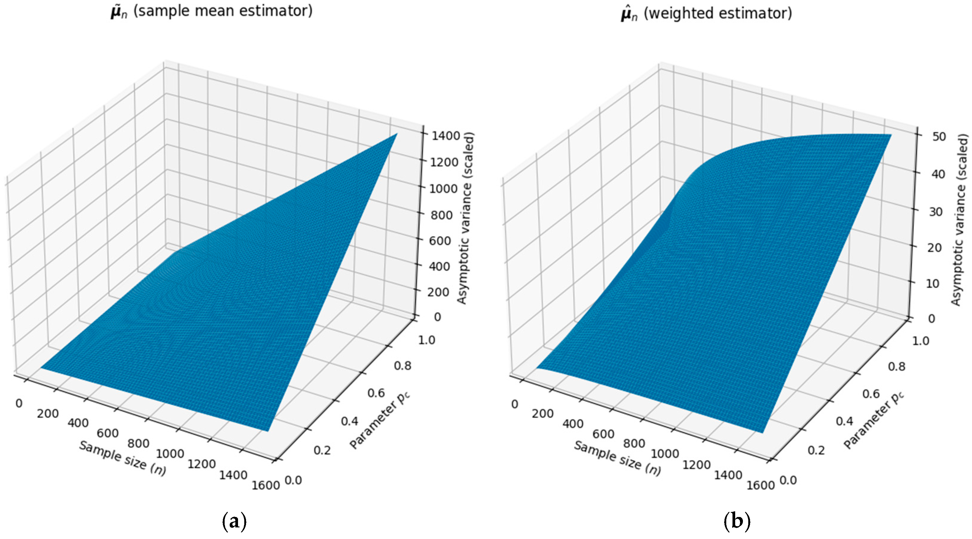
Therefore, the weighted estimator ${\widehat{\mathit{\mu }}}_{\mathit{n}}$ is asymptotically more efficient than the simple sample mean estimator ${\widehat{\mathit{\mu }}}_{\mathit{n}}$. This can also be seen in Figure 5, which shows 3D plots of both asymptotic variances, viewed as functions of the variables $p_c\in \left(\mathrm{0,1}\right)$ and $n>0$. Note that the covariance matrix $\Sigma$ is factored here, i.e., the surfaces represent the scalar part of the asymptotic variances.

Figure 5. 3D plots of asymptotic variances of the estimate ${\tilde{\mathit{\mu }}}_{\mathit{n}}$ (a) and estimate ${\widehat{\mathit{\mu }}}_{\mathit{n}}$ (b), depending on parameter $p_c\in \left(\mathrm{0,1}\right)$ and sample size $n>0$.

5. Numerical Simulation and Application

Two important aspects related to the practical implementation of the 2D-GSB process are examined here. First, numerical Monte Carlo simulations of the basic series of the 2D-GSB model are carried out, for which the previously described estimators are calculated, and their efficiency is analyzed. Then, based on real data, the application of the 2D-GSB process is presented in the analysis of the dynamics and empirical distributions of the total number of different forms of criminal offenses in the Republic of Serbia.

5.1. Numerical Simulations of the 2D-GSB Estimates

This section describes the estimation of the parameters of the 2D-GSB model, based on $S=300$ independent Monte Carlo replications of the basic 2D-GSB series. In the first step, a series of innovations ${\mathit{\epsilon }}_{\mathit{t}}={\left({\epsilon }_t^{\left(1\right)},{\epsilon }_t^{\left(2\right)}\right)}^{\mathrm{\top }}$ are generated as independent and identically distributed vectors with two-dimensional normal distribution $\mathcal{N}\left(0,\Sigma \right)$, and thereafter, the indicator series $q_t\left(c\right)$, defined as in Equation (4), is easily determined. According to this, the basic 2D-GSB series $\left({\mathit{Y}}_{\mathit{t}}\right)$ is constructed, with the mean vector ${\mathit{\mu }}_{\mathbf{0}}={({\mu }_0^{\left(1\right)},{\mu }_0^{\left(2\right)})}^{\mathrm{\top }},$ as well as the bivariate increments $\left({\mathit{X}}_{\mathit{t}}\right)$, which are used for estimation of the unknown parameters $\theta ={\left(p_c,{\sigma }_1^2, {\sigma }_2^2, \rho \right)}^{\mathrm{\top }}.$ The numerical simulations are designed to examine the finite-sample behavior of the proposed estimators and to verify the theoretical results derived in Section 4. In particular, the Monte Carlo study focuses on the accuracy, stability, and asymptotic properties of the estimators under repeated sampling from the 2D-GSB process. In doing so, for the basic series $\left({\mathit{Y}}_{\mathit{t}}\right)$ the mean vector ${\mathit{\mu }}_{\mathbf{0}}={({\mu }_0^{\left(1\right)},{\mu }_0^{\left(2\right)})}^{\mathrm{\top }}={\left(\mathrm{0,1}\right)}^{\mathrm{\top }}$ is taken, and for the threshold parameter the value $c=4$ is chosen, as well as for the covariance matrix:

$$\Sigma =\left[\begin{array}{cc}{\sigma }_1^2& \rho {\sigma }_1{\sigma }_2\\ \rho {\sigma }_1{\sigma }_2& {\sigma }_2^2\end{array}\right]=\left[\begin{array}{cc}1& 1\\ 1& 4\end{array}\right].$$

It is worth noting that then, according to the previous considerations (see Remark 3), the parameter $p_c$, defined by Equation (4), represents the survivor function of the mixture ${\mathsf{\chi }}_2^2$ distribution, which does not have a closed form. Thus, it is estimated here by an additional Monte Carlo experiment with $N=\mathrm{200,000}$ independent realizations. Note that using such extensive simulations, the estimated value of $p_c$ is obtained with high accuracy, so it can be used as a reference value. In this way, as the true values of the parameters, the vector ${\theta }_0={(p_c, {\sigma }_1^2, {\sigma }_2^2,\rho )}^{\mathrm{\top }}={(0.3967, 1, 4, 0.5)}^{\mathrm{\top }}$ is obtained.

The estimates of the vector ${\mathit{\mu }}_{\mathbf{0}}$ are calculated using estimators ${\tilde{\mathit{\mu }}}_{\mathit{n}}$ and ${\widehat{\mathit{\mu }}}_{\mathit{n}}$, defined by Equations (45) and (46), respectively. To this end, realizations of the series $\left({\mathit{Y}}_{\mathit{t}}\right)$ of length $n=150$ are observed, and descriptive statistics (Min, Mean, Max), along with the appropriate estimation errors, i.e., bias, standard deviation (StDev) and root mean-squared error (RMSE), of the estimates thus obtained are shown in Table 1. As mentioned above, due to the non-stationarity of the series $\left({\mathit{Y}}_{\mathit{t}}\right)$, estimates of the mean vector ${\mathit{\mu }}_{\mathbf{0}}$ have an unbounded asymptotic variance, so there is a large range of their observed values. Nevertheless, it is obvious that the estimator ${\widehat{\mathit{\mu }}}_{\mathit{n}}$ is more efficient than ${\tilde{\mathit{\mu }}}_{\mathit{n}}$, because its error statistics are significantly smaller. Furthermore, in order to investigate the asymptotic properties of the estimates thus obtained, they were also tested in relation to the AN property, and the results of these tests are also presented in Table 1. For this purpose, the following three statistical tests of normality were used:

Table 1. Descriptive statistics and AN testing results of the mean value estimates. (Series length is $n=150$, and the true parameter values are ${\mu }_0^{\left(1\right)}=0, {\mu }_0^{\left(2\right)}=1$).

Statistics	$\mathbf{Sample} \mathbf{Mean} \mathbf{Estimator} \left({\tilde{\mathit{\mu }}}_{\mathit{n}}\right)$		$\mathbf{Weighted} \mathbf{Estimator} \left({\widehat{\mathit{\mu }}}_{\mathit{n}}\right)$
	${\tilde{\mathit{\mu }}}_{\mathit{n}}^{\left(1\right)}$	${\tilde{\mathit{\mu }}}_{\mathit{n}}^{\left(2\right)}$	${\widehat{\mathit{\mu }}}_{\mathit{n}}^{\left(1\right)}$	${\widehat{\mathit{\mu }}}_{\mathit{n}}^{\left(2\right)}$
Min	−12.160	−22.467	−7.9302	−14.305
Mean	−0.0756	0.7713	−0.0569	0.9442
Max	16.408	27.833	10.318	16.982
Bias	−0.0756	−0.2287	−0.0569	−0.0558
StDev	4.3383	8.9660	2.7328	5.4760
RMSE	4.3317	8.9539	2.7289	5.4672
SW	0.9967	0.9970	0.9940	0.9971
($p$-value)	(0.8003)	(0.8571)	(0.2827)	(0.8695)
AD	0.1182	0.2874	0.3676	0.3367
($p$-value)	(0.9899)	(0.6182)	(0.4289)	(0.5042)
JB	1.2528	0.3156	2.8775	0.1155
($p$-value)	(0.5345)	(0.8540)	(0.2372)	(0.9439)

-

Shapiro–Wilk normality test (SW);

-

Anderson–Darling normality test (AN);

-

Jarque–Bera normality test (JB).

Test statistics, as well as their corresponding $p$-values (listed in parentheses above), were calculated using procedures from the R-4.5.2 package “nortest” [33]. It is evident that both estimators ${\tilde{\mathit{\mu }}}_{\mathit{n}}$ and ${\widehat{\mathit{\mu }}}_{\mathit{n}}$ have the AN property, even though they are obtained from the realization of a non-stationary series $\left({\mathit{Y}}_{\mathit{t}}\right)$. It should be noted that this is closely related to Theorems 4 and 5, which, among others, describe AN properties of scaled processes based on the observed GSB series $\left({\mathit{Y}}_{\mathit{t}}\right)$.

Further, the MoM estimates of the true parameter ${\theta }_0$ are simply obtained by using Equations (26)–(28), while the ECF estimates are calculated by minimizing the integral given by Equation (36). Hence, similarly as in Milovanović [34], the well-known Gauss-Hermite cubature are used, with the weight function $g\left(u_1, u_2\right)=\exp \left(-{‖u_1‖}^2-{‖u_2‖}^2\right),$ $u_1, u_2\in {\mathbb{R}}^2,$ and 81 cubature nodes, where the entire procedure is obtained using the R-4.5.2 package “statmod” [35]. Thereafter, taking the previously obtained MoM estimates as initial values, the objective function given by Equation (36) is minimized using the constrained optimization procedure “L-BFGS-B” [36], also implemented in the statistical programming language “R”. Finally, in order to examine the efficiency, as well as other previously mentioned asymptotic properties of the estimates thus obtained, different series lengths $n\in \left\{150, 500, 1500\right\}$ are considered. Their basic descriptive statistics, along with statistics and $p$-values of the aforementioned normality tests, are also calculated in the statistical software “R” and presented in the following Table 2, Table 3 and Table 4.

Table 2. Descriptive statistics and AN testing results of estimated parameter values. (Series length is $n=150$, and the true parameter values are $p_c\approx 0.3967$, ${\sigma }_1^2=1$, ${\sigma }_1^2=4, \rho =0.5$).

Statistics	MoM				ECF
	${\mathit{p}}_{\mathit{c}}$	${\mathit{\sigma }}_1^2$	${\mathit{\sigma }}_2^2$	$\mathit{\rho }$	${\mathit{p}}_{\mathit{c}}$	${\mathit{\sigma }}_1^2$	${\mathit{\sigma }}_2^2$	$\mathit{\rho }$
Min	0.0000	0.6768	2.7087	0.2738	0.0944	0.5628	2.8580	0.2820
Mean	0.3846	0.9845	4.0192	0.4973	0.3872	0.9987	4.0186	0.4982
Max	0.7135	1.3562	6.3611	0.6745	0.8229	1.4708	5.6043	0.7675
Bias	−0.0121	−0.0155	0.0192	−0.0027	−0.0095	−0.0013	0.0186	−0.0018
StDev	0.1407	0.1381	0.6353	0.0785	0.1579	0.1618	0.5839	0.0862
MSE	0.1407	0.1384	0.6334	0.0784	0.1580	0.1613	0.5823	0.0860
SW	0.986 **	0.995	0.985 **	0.994	0.980 *	0.996	0.984 **	0.992
($p$-value)	(0.005)	(0.376)	(0.004)	(0.329)	(0.026)	(0.735)	(0.002)	(0.083)
AD	0.850 *	0.446	0.753 *	0.261	0.933 *	0.333	0.883 *	0.602
($p$-value)	(0.028)	(0.281)	(0.049)	(0.706)	(0.018)	(0.509)	(0.024)	(0.117)
JB	6.502 *	2.066	8.054 *	2.502	4.272	0.556	12.676 **	4.816
($p$-value)	(0.039)	(0.356)	(0.018)	(0.286)	(0.118)	(0.757)	(0.002)	(0.090)

* $p<0.05$, ** $p<0.01.$

Table 3. Descriptive statistics and AN testing results of estimated parameter values. (Series length is $n=500$, and the true parameter values are the same as in Table 2).

Statistics	MoM				ECF
	${\mathit{p}}_{\mathit{c}}$	${\mathit{\sigma }}_1^2$	${\mathit{\sigma }}_2^2$	$\mathit{\rho }$	${\mathit{p}}_{\mathit{c}}$	${\mathit{\sigma }}_1^2$	${\mathit{\sigma }}_2^2$	$\mathit{\rho }$
Min	0. 0794	0.7787	3.2927	0.3459	0.1409	0.8423	3.3609	0.3657
Mean	0.3984	1.0102	3.9947	0.4959	0.3953	1.0056	3.9953	0.4988
Max	0.6012	1.2533	4.8995	0.6066	0.5941	1.2592	4.8769	0.6025
Bias	0.0017	0.0102	−0.0053	−0.0041	−0.0014	0.0056	−0.0047	−0.0012
StDev	0.0722	0.1018	0.3350	0.0464	0.0884	0.0876	0.2995	0.0438
MSE	0.0720	0.1019	0.3339	0.0466	0.0884	0.0875	0.2986	0.0437
SW	0.978 *	0.991	0.984	0.991	0.991	0.997	0.988	0.992
($p$-value)	(0.016)	(0.478)	(0.074)	(0.497)	(0.505)	(0.983)	(0.214)	(0.536)
AD	0.699	0.456	0.468	0.462	0.526	0.186	0.375	0.452
($p$-value)	(0.067)	(0.263)	(0.247)	(0.254)	(0.178)	(0.904)	(0.410)	(0.270)
JB	5.984	1.186	2.454	1.632	0.433	0.313	2.271	2.047
($p$-value)	(0.050)	(0.553)	(0.293)	(0.442)	(0.805)	(0.855)	(0.321)	(0.359)

* $p<0.05.$

Table 4. Descriptive statistics and AN testing results of estimated parameter values. (Series length is $n=1500$, and the true parameter values are the same as in Table 2 and Table 3).

Statistics	MoM				ECF
	${\mathit{p}}_{\mathit{c}}$	${\mathit{\sigma }}_1^2$	${\mathit{\sigma }}_2^2$	$\mathit{\rho }$	${\mathit{p}}_{\mathit{c}}$	${\mathit{\sigma }}_1^2$	${\mathit{\sigma }}_2^2$	$\mathit{\rho }$
Min	0.2588	0.8597	3.5807	0.4272	0.2806	0.8698	3.6226	0.4376
Mean	0.3984	1.0051	4.0355	0.5010	0.3969	1.0047	4.0264	0.5006
Max	0.4968	1.1618	4.5975	0.5644	0.5454	1. 1595	4.5100	0.5575
Bias	0.0017	0.0051	0.0355	0.0010	0.0002	0.0047	0.0264	0.0006
StDev	0.0471	0.0529	0.1983	0.0240	0.0418	0.0504	0.1775	0.0235
MSE	0.0469	0.0529	0.2008	0.0239	0.0418	0.0504	0.1789	0.0234
SW	0.997	0.992	0.994	0.997	0.994	0.995	0.994	0.997
($p$-value)	(0.784)	(0.111)	(0.326)	(0.854)	(0.224)	(0.359)	(0.335)	(0.755)
AD	0.315	0.627	0.415	0.215	0.722	0.445	0.404	0.329
($p$-value)	(0.542)	(0.101)	(0.333)	(0.846)	(0.059)	(0.282)	(0.354)	(0.514)
JB	0.476	5.018	2.232	0.469	0.549	2.434	2.823	0.300
($p$-value)	(0.788)	(0.081)	(0.328)	(0.791)	(0.760)	(0.296)	(0.244)	(0.861)

The results thus reported indicate that both estimation procedures perform satisfactorily even for moderate sample sizes. The empirical means of all estimated parameters are very close to their true values, while the corresponding biases remain small and mainly decrease as the sample size increases. A mild non-monotonic behavior of the finite-sample accuracy can be observed for the variance parameter ${\sigma }_2^2$, which is typical for mixture-type models. Additionally, within the 2D-GSB framework, variance parameters enter both the dispersion structure and the regime-selection probability $p_c$, which depends implicitly on the matrix $\Sigma$. Overall, as expected, the dispersion of the estimates measured through standard deviations and mean squared errors generally decreases as the sample size increases. For larger samples, including the longest series considered ($n=1500$), the estimates exhibit small bias and moderate variability across all parameters, supporting their suitability for empirical applications based on longer time series.

Overall, the simulation results indicate that both estimation approaches perform satisfactorily across different sample sizes. The MoM procedure is computationally straightforward and particularly suitable for quick preliminary estimation or large datasets, due to its closed-form structure. In contrast, the ECF approach involves higher computational cost but exhibits stronger asymptotic efficiency properties. The results reported in Table 2, Table 3 and Table 4 suggest that the ECF estimator tends to achieve slightly lower dispersion and mean squared error in moderate samples, whereas MoM remains stable and practically convenient. This trade-off highlights the complementary roles of the two procedures in applied implementation. Also, note that in practical implementation, the threshold parameter $c$ can be determined either via its theoretical one-to-one relationship with $p_c$ or through a quantile-based calibration of the innovation norm. This ensures a transparent and data-driven specification of regime activation.

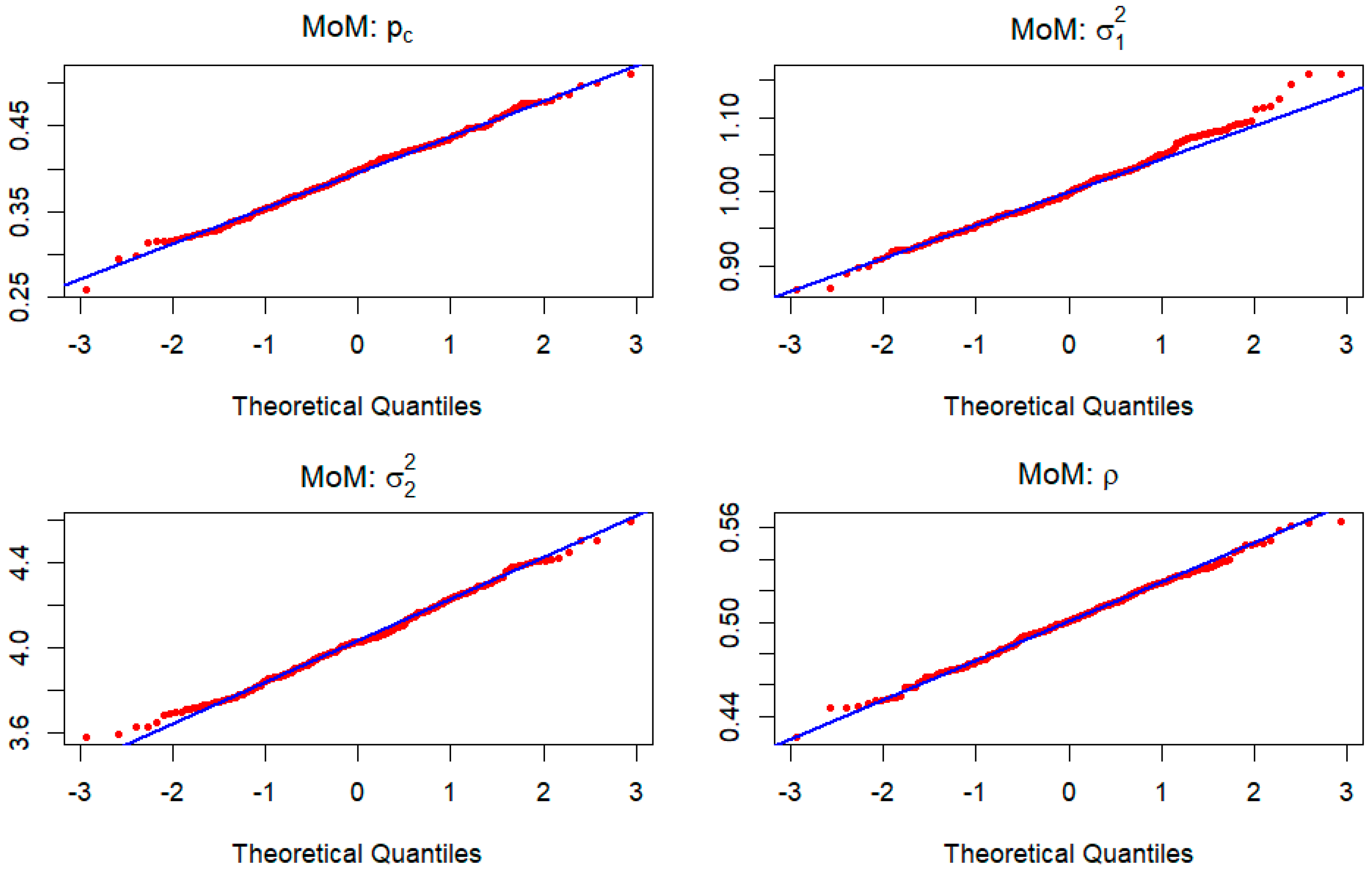
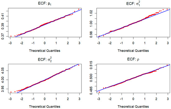
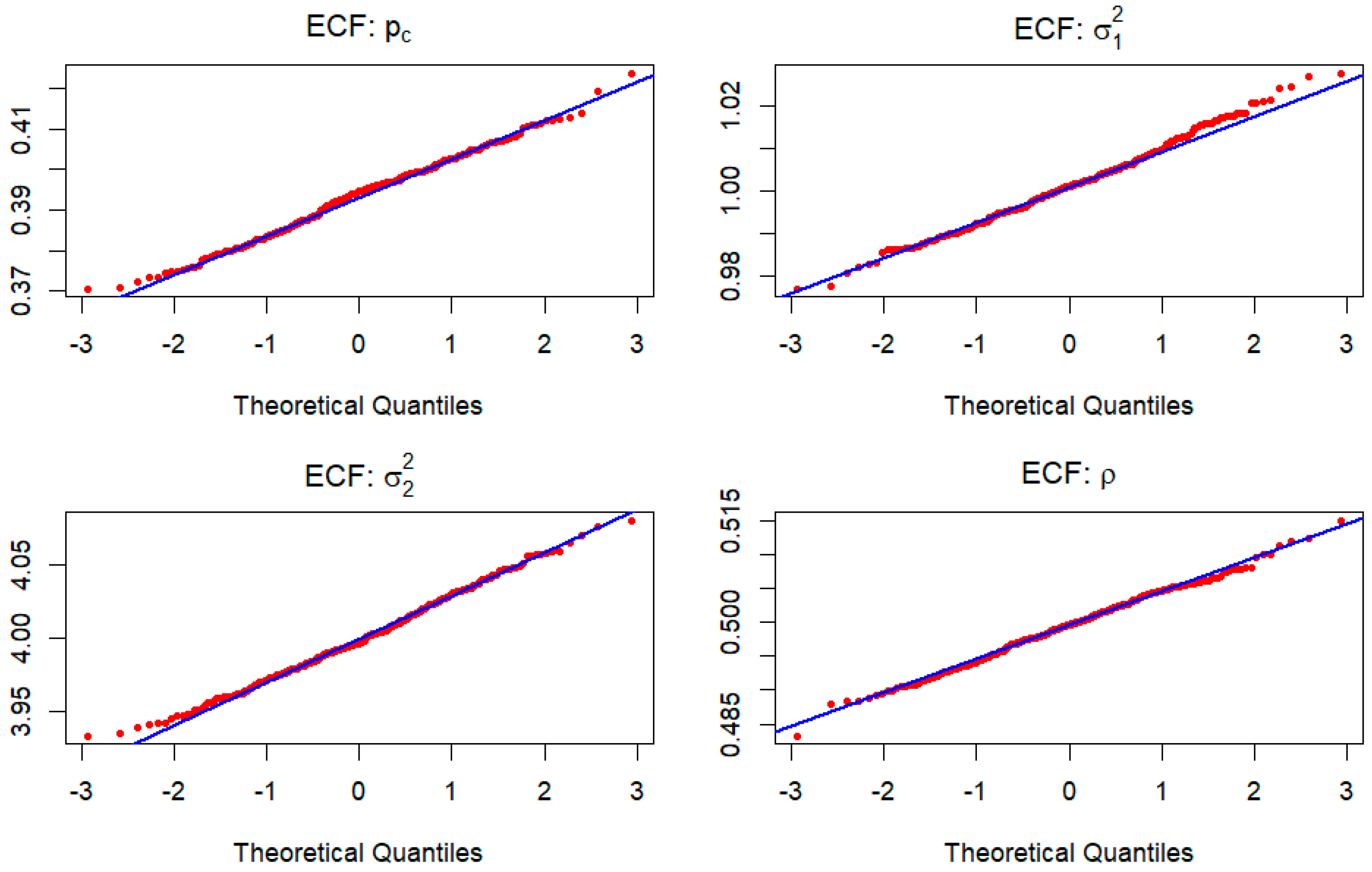
Finally, note that although the model is derived under Gaussian innovation assumptions, the mixture-based structure provides a degree of robustness to moderate deviations from normality, as reflected in the empirical application. As an illustration, Figure 6 and Figure 7 display the Q–Q plots of the empirical distributions of the estimated parameters against the corresponding Gaussian quantiles for $n=1500$. The plots provide graphical support for the asymptotic normality of both estimation procedures and indicate a slightly improved finite-sample behavior of the ECF estimators. In this way, these graphical representations are consistent with the theoretical asymptotic results and with the variance and RMSE comparisons shown in Table 2, Table 3 and Table 4. In general, the Monte Carlo results confirm the above-mentioned theoretical properties of the 2D-GSB estimator and provide the possibility of their applicability in practical, multivariate time series analysis.

Figure 6. Q–Q plots of the empirical distributions of the MoM estimates ${\widehat{p}}_c$, ${\widehat{\sigma }}_1^2$, ${\widehat{\sigma }}_2^2$, and $\widehat{\rho }$, obtained from $S=300$ Monte Carlo replications of the 2D-GSB process with sample size $n=1500$.

Figure 7. Q–Q plots of the empirical distributions of the ECF estimates ${\widehat{p}}_c$, ${\widehat{\sigma }}_1^2$, ${\widehat{\sigma }}_2^2$, and $\widehat{\rho }$, based on $S=300$ Monte Carlo replications with sample size $n=1500$.

5.2. Application: A Case Study of Crime Dynamics

After determining the properties of the proposed estimators over finite samples through Monte Carlo simulations, we consider here the empirical application of the 2D-GSB framework. To illustrate the practical performance of the proposed model, we apply it to real-world multivariate time series representing the total number of specific criminal offenses committed on the territory of the Republic of Serbia. The data were obtained based on official records of the Ministry of Internal Affairs of the Republic of Serbia, which are monitored daily, starting from 1 January 2015 and ending with 31 December 2024, which resulted in a time series length of $n=3653$. It should be noted that each of the observed series is obtained and classified according to the official Criminal Code of the Republic of Serbia (code KD_xxx), where bivariate series contain data on related criminal activities as their components. In this way, two bivariate series are observed, designated as Series A and Series B, whose components are the following:

A₁: Petty theft (code KD_203).

A₂: Aggravated theft and robbery (code KD_204).

B₁: Counterfeiting money, securities, counterfeiting and misuse of payment cards (codes KD_241-244).

B₂: Document falsification and other special cases of document falsification (codes KD_355-357).

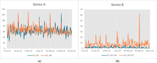
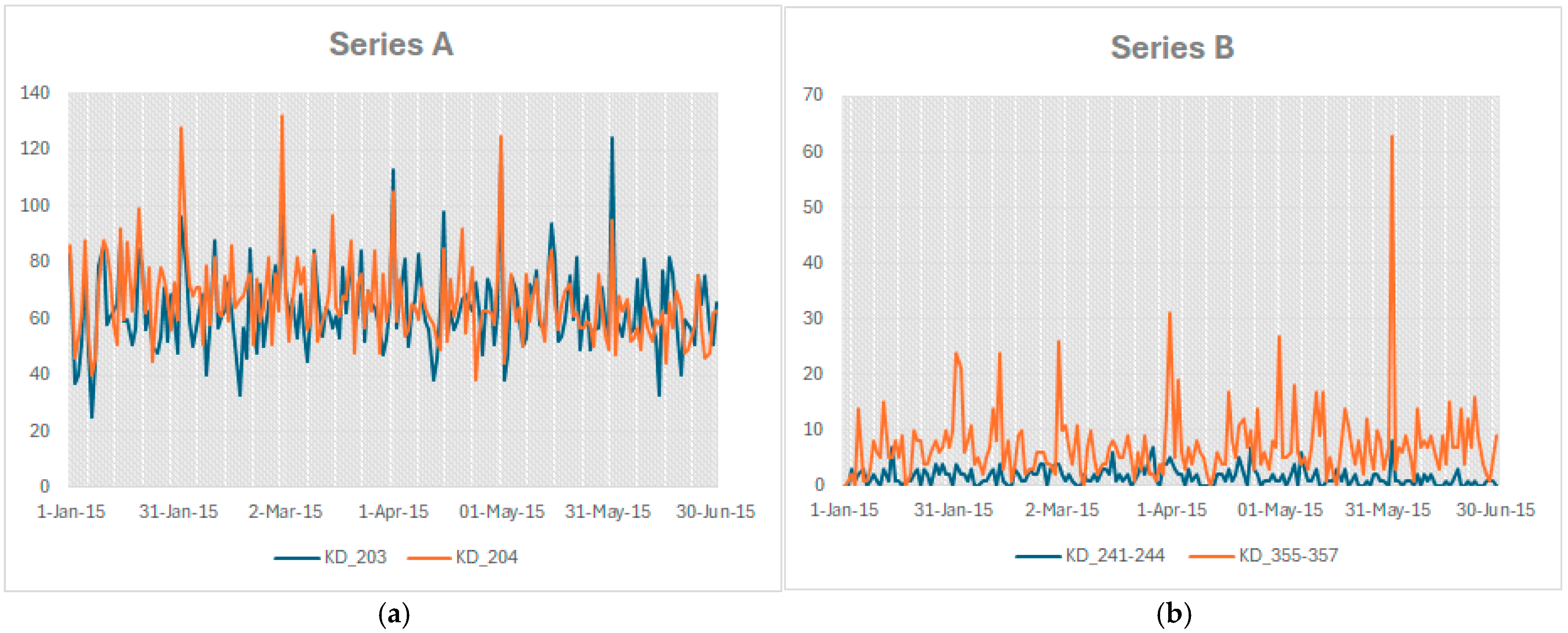
The dynamics of both bivariate time series are illustrated in Figure 8, where the pronounced fluctuations, i.e., sudden “jumps” in the number of committed criminal acts, are clearly visible. At the same time, the intercorrelation between the components of both bivariate series is noticeable even at first glance. Therefore, use of a synchronized threshold mechanism is particularly suitable in this context, as external shocks (e.g., policy changes, economic disturbances, or enforcement actions) may simultaneously affect related crime categories. The common regime indicator thus provides a natural interpretation of coordinated spikes and structural shifts observed in the data. Note that although the observed series represent daily crime counts, the proposed 2D-GSB model is not intended to directly model the count-valued observation space, but rather to capture the underlying common dynamics of pronounced fluctuations and synchronized regime changes.

Figure 8. Dynamics of the total number of two types of theft (a) and forgery (b) on the territory of the Republic of Serbia.

In this context, the descriptive statistics reported in Table 5 reveal a pronounced overdispersion of both series (especially Series A), as well as extremely heavy-tailed behavior, reflected in very high kurtosis and skewness in Series B. In addition, the average value of document forgeries (component B₂) is approximately 7.3 per day, but the range varies from as few as 0 to as many as 304 such crimes per day. Along with the significant cross-dependence between their components, these features motivate the use of a latent regime-based framework rather than standard count-based models. Also, in contrast to univariate approaches, the two-dimensional GSB framework enables the joint modeling of related crime categories while explicitly accounting for cross-dependence in their extreme dynamics.

Table 5. Basic statistical indicators of observed real-world data.

Statistics	A1	A2	B1	B2
Min	3	4	0	0
Mean	47.13	35.14	1.677	7.306
Median	46	31	1	6
Mode	44	23	0	6
Max	152	162	87	304
Variance	205.1	289.7	8.049	88.79
Kurtosis	5.634	3.109	268.0	399.8
Skewness	1.366	1.319	11.37	16.14
Range	149	158	87	304
Correlation	0.6566		0.3391

Since the original series represent crime counts and exhibit pronounced heteroscedasticity and skewness, a logarithmic transformation (“log-volume”) is applied prior to modeling. This transformation not only stabilizes the variance and reduces asymmetry but also facilitates a closer approximation of the increment process by a Gaussian mixture distribution, as assumed in the 2D-GSB framework. Consequently, the transformed increment series is more consistent with the underlying distributional structure of the model. For these reasons, as basic bivariate series $\left({\mathit{Y}}_{\mathit{A},\mathit{t}}\right)$ and $\left({\mathit{Y}}_{\mathit{B},\mathit{t}}\right)$, the realizations of the so-called log-volumes, i.e., logarithmic values of series A and B, are observed as follows:

$$Y_{A,t}^{\left(i\right)}:=\ln \left(A_{i,t}\right), Y_{B,t}^{\left(i\right)}:=\ln \left(1+B_{i,t}\right), i=0,1.$$

(47)

As is stated in [37,38], the main goal of these transformations is to more evenly obtain values of both series, while based on increasing of the logarithmic function, the emphasis of fluctuations will remain. Additionally, note that, unlike the series ${\mathit{Y}}_{\mathit{A},\mathit{t}}={(Y_{A,t}^{\left(1\right)},Y_{A,t}^{\left(2\right)})}^{\mathrm{\top }}$, which represents the usual log-transformation, the series ${\mathit{Y}}_{\mathit{B},\mathit{t}}={(Y_{B,t}^{\left(1\right)},Y_{B;t}^{\left(2\right)})}^{\mathrm{\top }}$ is a so-called shifted log-transformation, as a consequence of the equality $\min \left(B_1\right)=\min \left(B_2\right)=0$. In this way, from inequalities $A\ge 1$ and $B\ge 0$, it follows that both series of log-volumes are non-negative $\left({\mathit{Y}}_{\mathit{A},\mathit{t}},{\mathit{Y}}_{\mathit{B},\mathit{t}}\ge 0\right)$.

Further, using the log-volumes as a basic bivariate series, the location parameter ${\mathit{\mu }}_{\mathbf{0}}$ for both series is estimated, following the procedure described in Section 4.3. In more detail, the $\mu$-estimates are obtained according to Equations (45) and (46), which correspond, respectively, to the sample and weighted mean values of the bivariate series $\left({\mathit{Y}}_{\mathit{A},\mathit{t}}\right),\left({\mathit{Y}}_{\mathit{B},\mathit{t}}\right)$. Using Equations (11) and (12), the increment series $\left({\mathit{X}}_{\mathit{A},\mathit{t}}\right)$ and $\left({\mathit{X}}_{\mathit{B},\mathit{t}}\right)$ are then constructed. Based on these series, the remaining parameters collected in the vector $\mathit{\theta }$ are estimated, including the probability of exceeding the threshold and the elements of the covariance matrix. To this end, the procedures presented in Section 4.1 and Section 4.2 are applied, namely the method of moments (MoM) and empirical characteristic functions (ECF) method, thus ensuring consistency with the theoretical framework developed previously.

The resulting estimates reported in Table 6 demonstrate stability and interpretability, thereby enabling further analysis of different crime categories. In particular, the series-specific $\mu$-estimates reflect systematic differences in the average growth rates of the corresponding crime categories. At the same time, the estimated $\theta$-parameters suggest substantial variability and cross-dependence in the increment dynamics, justifying the use of a multivariate threshold-based model. Note that the magnitudes of the estimated parameters remain stable and interpretable across estimation methods, supporting the adequacy of the proposed inference framework. The modest differences between the MoM and ECF estimates remain within a comparable range and do not change the overall structural interpretation.

Table 6. Estimated parameter values of the 2D-GSB process.

$\mathit{\mu }$—Estimates	${\mathit{Y}}_{\mathit{A},\mathit{t}}^{\left(1\right)}$	${\mathit{Y}}_{\mathit{A},\mathit{t}}^{\left(2\right)}$	${\mathit{Y}}_{\mathit{B},\mathit{t}}^{\left(1\right)}$	${\mathit{Y}}_{\mathit{B},\mathit{t}}^{\left(2\right)}$
${\tilde{\mathit{\mu }}}_{\mathit{n}}$	3.808	3.450	0.7368	1.903
${\widehat{\mathit{\mu }}}_{\mathit{n}}$	3.946	3.789	0.6741	1.949
$\mathit{\theta }$—Estimates	MoM	ECF	MoM	ECF
${\widehat{\mathit{p}}}_{\mathit{c}}$	0.1290	0.1296	0.1345	0.1626
$\widehat{\mathit{c}}$	0.2574	0.2320	1.467	1.322
${\widehat{\mathit{\sigma }}}_1^2$	0.0566	0.0589	0.3875	0.3445
${\widehat{\mathit{\sigma }}}_2^2$	0.0680	0.0857	0.8426	0.8357
$\widehat{\mathit{\rho }}$	0.3698	0.3618	0.1478	0.1707

From an interpretative perspective, the estimated parameters provide additional insight into the structural dynamics of the analyzed crime categories. For Series A (petty theft and aggravated theft/robbery), the estimated probability ${\widehat{p}}_c\approx 0.13$ suggests that coordinated shock-activated episodes occur in roughly 13% of observations, indicating recurrent but not dominant structural fluctuations affecting both offense types simultaneously. In contrast, for Series B (counterfeiting-related offenses and document falsification), the estimated probabilities range between 0.13 and 0.16, implying a comparable frequency of coordinated disturbances. However, the substantially higher estimated threshold $\widehat{c}$ (approximately 1.3–1.5, compared to 0.23–0.26 in Series A) indicates that more pronounced innovation magnitudes are required to trigger regime activation in financial and document-related crimes. This suggests that while synchronized shifts occur with similar frequency across both crime groups, the intensity of shocks necessary to activate such shifts differs, reflecting potentially distinct structural sensitivity patterns within the two categories.

To further assess the empirical adequacy of the proposed model, we compare the 2D-GSB specification with a standard first-order vector auto-regression (VAR(1)) benchmark estimated on the stationary increment series $\left({\mathit{X}}_{\mathit{A},\mathit{t}}\right)$ and $\left({\mathit{X}}_{\mathit{B},\mathit{t}}\right)$. Table 7 reports the corresponding log-likelihood (LogLik), Akaike and Bayesian information criteria (AIC and BIC), together with the joint root mean square error (RMSE) for both models and both series. The joint RMSE is defined as the square root of the arithmetic mean of the component-wise mean squared deviations between empirical and fitted densities, thereby providing a single aggregate measure of distributional fit. As can be seen, the 2D-GSB model achieves higher log-likelihood values and lower information criteria and discrepancy measures than the standard VAR(1) specification. It is also worth noting that the proposed 2D-GSB framework involves only four parameters, compared to seven in the VAR model. These results indicate a more parsimonious yet substantially improved distributional fit of the increment process, particularly in the case of Series A.

Table 7. Goodness-of-fit statistics of VAR(1) and 2D-GSB benchmarks.

Statistics	Series A		Series B
	VAR(1)	2D-GSB	VAR(1)	2D-GSB
LogLik	−1339.1	−1154.9	−8031.5	−7863.4
AIC	2692.2	2317.8	16,077.1	15,734.7
BIC	2735.6	2342.6	16,120.5	15,759.5
RMSE	0.0105	7.56$\times {10}^{-3}$	0.0237	0.0209

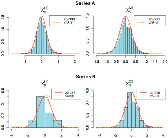
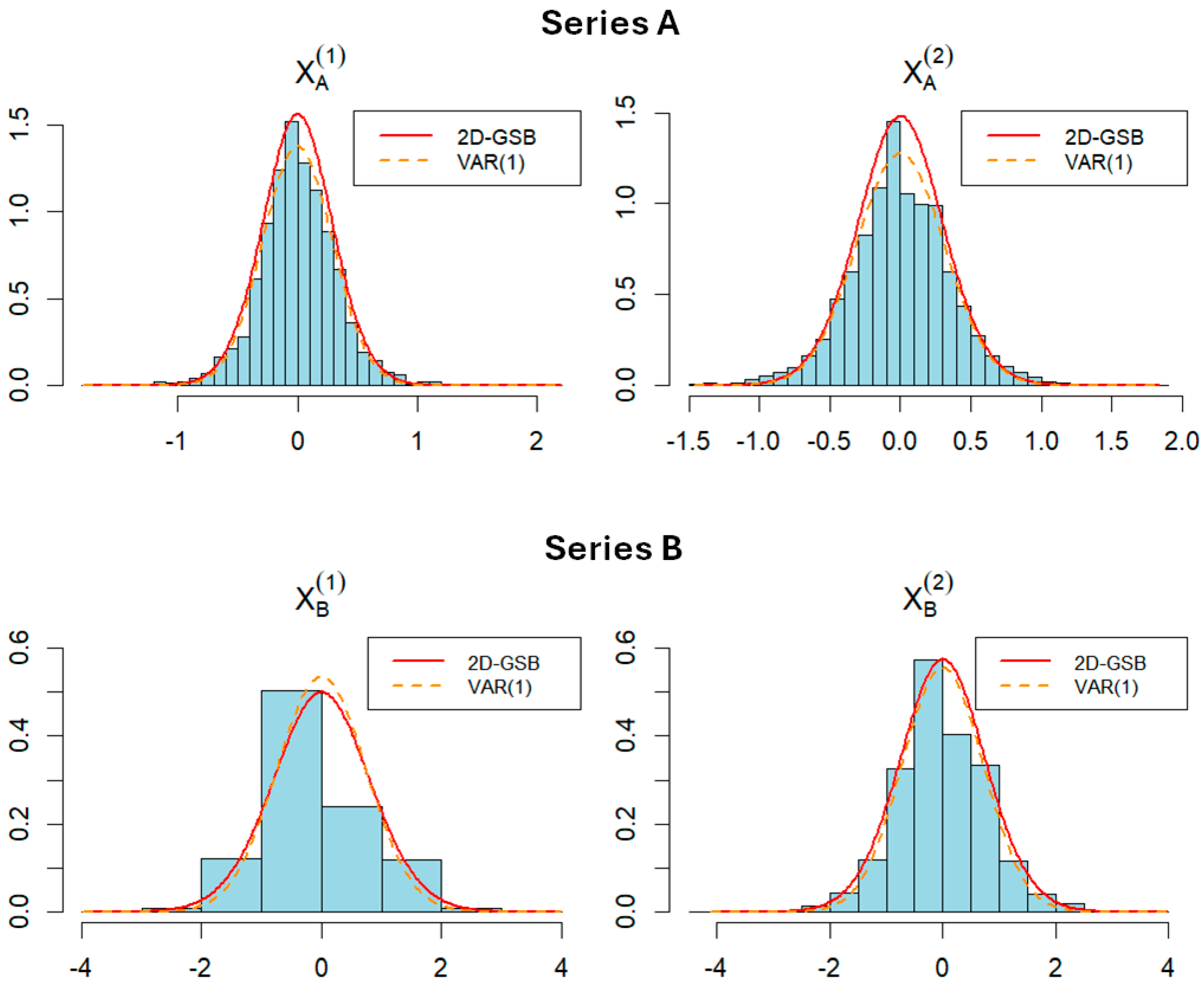
In addition, Figure 9 presents the empirical marginal distributions of the bivariate increments together with the Gaussian fit implied by the VAR(1) specification and the Gaussian mixture of the increments implied by the 2D-GSB model introduced in Section 3. The VAR(1) estimation is carried out using the R-4.5.2 package “vars” [39], while the 2D-GSB parameters are obtained via the MoM procedure for Series A and the ECF method for Series B, as described previously. As illustrated in the figure, the mixture representation underlying the increments of the 2D-GSB model provides a closer alignment with the empirical distributions, particularly in capturing increased dispersion and heavier-tail behavior. In contrast, the single-Gaussian structure of the VAR(1) model tends to underestimate the probability of extreme observations in most cases. Overall, the visual agreement between the empirical histograms and the fitted mixture densities further supports the adequacy of the 2D-GSB framework for modeling synchronized regime dynamics in the observed data.

Figure 9. Empirical distributions of the stationary series of increments (histograms) along with their fitted PDFs obtained using VAR(1) and 2D-GSB model (lines): Series A—plots above; Series B—plots below.

Further, fitting of the empirical distributions of the underlying Series A and B is carried out. Due to the distinct transformations in Equation (47), the implied distributions of these series differ. While Series A follows a mixture of bivariate log-normal distributions, Series B is characterized by a mixture of shifted bivariate log-normal distributions. In both cases, the Jacobian of the inverse transformation plays a crucial role, ensuring a proper mapping from the latent Gaussian mixture to the observable crime counts. Thus, the fitted distributions of the original crime series are obtained by an explicit change-of-variables procedure based on the transformations defined in Equation (47).

Let ${\mathit{Y}}_{\mathit{t}}\in \left\{{\mathit{Y}}_{\mathit{A},\mathit{t}},{\mathit{Y}}_{\mathit{B},\mathit{t}}\right\}$ denote either of the latent processes given by Equation (47). From the theoretical results in Section 3, ${\mathit{Y}}_{\mathit{t}}$ follows a discrete mixture of bivariate Gaussian distributions

$$f_{{\mathit{Y}}_{\mathit{t}}}(\mathbf{y})=\sum _{k=0}^t\left({\displaystyle \genfrac{}{}{0pt}{}{t}{k}}\right)p_c^k(1-p_c{)}^{t-k}\varphi \left(\mathbf{y};{\mathit{\mu }}_{\mathbf{0}},\left(k+1\right)\Sigma \right),$$

where $\varphi \left(\mathbf{y};{\mathit{\mu }}_{\mathbf{0}},\left(k+1\right)\Sigma \right)$ is the PDF of the bivariate Gaussian distribution. Thus, for Series A, the inverse transformation ${\mathbf{A}}_t=\exp \left({\mathit{Y}}_{\mathit{A},\mathit{t}}\right)$ yields the density

$$f_{{\mathbf{A}}_t}(\mathbf{a})=f_{{\mathit{Y}}_{A,t}}\left(\ln \mathbf{a}\right) \left|\det {\displaystyle \frac{\mathsf{\partial }\ln \mathbf{a}}{\mathsf{\partial }\mathbf{a}}}\right|=\sum _{k=0}^t\left({\displaystyle \genfrac{}{}{0pt}{}{t}{k}}\right)p_c^k(1-p_c{)}^{t-k}{\displaystyle \frac{\varphi \left(\ln \mathbf{a};{\mathit{\mu }}_{\mathit{A}},\left(k+1\right){\Sigma }_A\right)}{a_1{a}_2}},$$

where $\mathbf{a}={\left(a_1,a_2\right)}^{\mathrm{\top }}>\mathbf{0}.$ Similarly, for Series B, using the inverse map ${\mathbf{B}}_t=\mathrm{e}\mathrm{x}\mathrm{p}\left({\mathit{Y}}_{\mathit{B},\mathit{t}}\right)-1$, the resulting density is given by

$$f_{{\mathbf{B}}_t}(\mathbf{b})=f_{Y_{B,t}}(\mathrm{l}\mathrm{n}(\mathbf{b}+\mathbf{1}))\left|\det {\displaystyle \frac{\mathsf{\partial }\ln \left(\mathbf{b}+\mathbf{1}\right)}{\mathsf{\partial }\mathbf{b}}}\right|=\sum _{k=0}^t\left({\displaystyle \genfrac{}{}{0pt}{}{t}{k}}\right)p_c^k(1-p_c{)}^{t-k}{\displaystyle \frac{\varphi \left(\ln \left(\mathbf{b}+\mathbf{1}\right);{\mathit{\mu }}_{\mathit{B}},\left(k+1\right){\Sigma }_B\right)}{\left(1+b_1\left)\right(1+b_2\right)}},$$

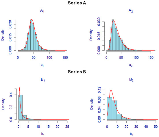
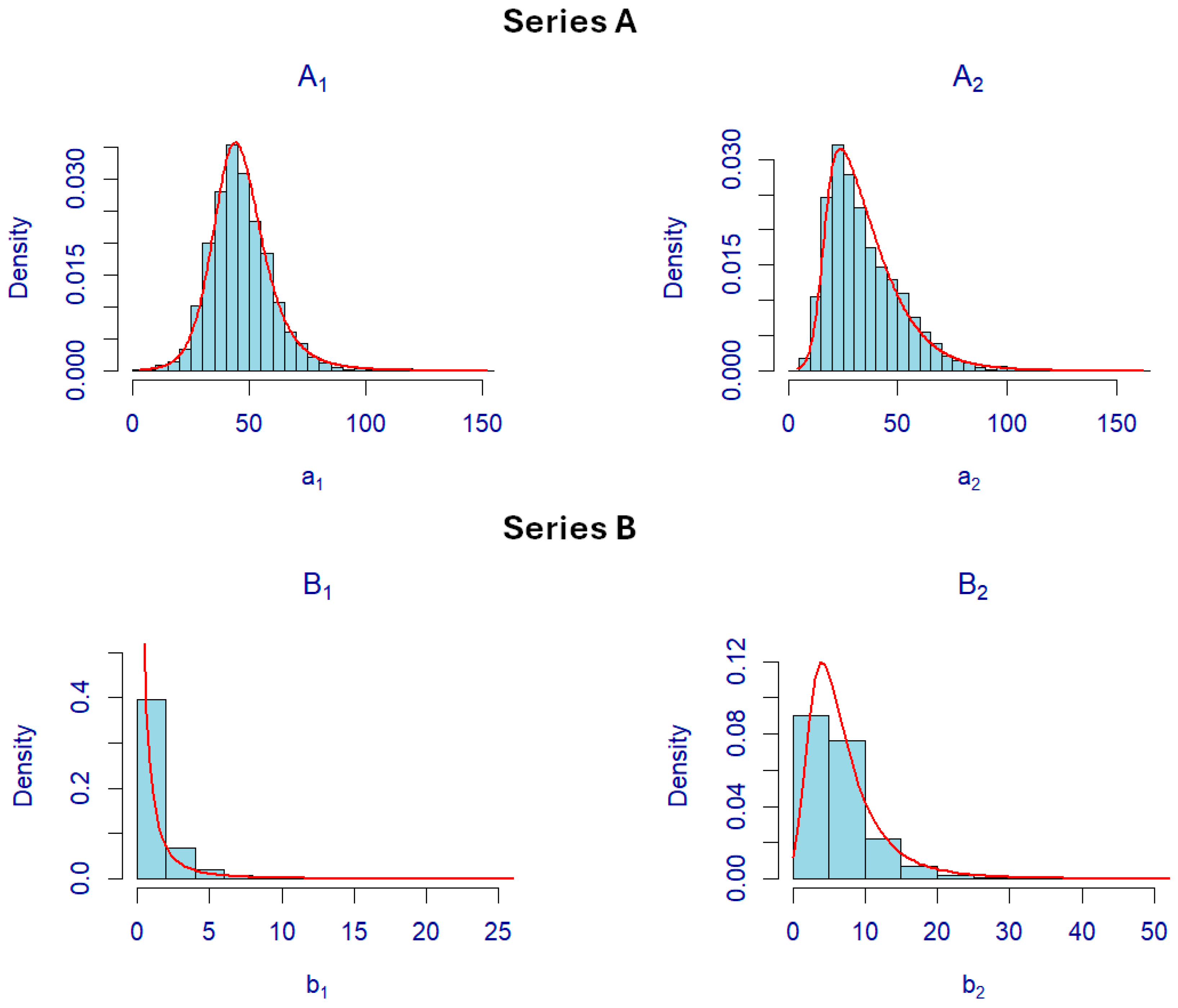
where $\mathbf{b}={\left(b_1,b_2\right)}^{\mathrm{\top }}\ge \mathbf{0}.$ Thus, the proposed framework induces a mixture of bivariate log-normal distributions for Series A and a mixture of shifted bivariate log-normal distributions for Series B, providing a link between the latent 2D-GSB dynamics and empirical distributions of observed crime counts. Nevertheless, it is worth noting that due to the non-stationarity of the mentioned series, which also depend on time $\left(t\right)$, it is necessary to apply some numerical procedures to calculate their PDFs. For this purpose, the R-4.5.2 package “distr” [40] is used, and the results of the applied procedure are shown in Figure 10.

Figure 10. Empirical distributions of crime dynamics data (histograms) and their fitted PDFs (lines), obtained by the proposed estimation procedure: Series A—plots above; Series B—plots below.

As illustrated in Figure 10, the empirical distributions of the original crime counts are shown together with the fitted theoretical densities obtained via the inverse-log mixture representations implied by the 2D-GSB model. For Series A (theft-related offenses), the fitted log-normal mixtures capture both the central mass and the pronounced right tails of the distributions, indicating that the proposed model adequately reflects the observed variability and intermittency. Similarly, for Series B (counterfeiting-related offenses), the shifted log-normal mixtures provide a satisfactory approximation of the highly skewed empirical distributions, particularly in the lower-count region and the gradual tail decay. Overall, the agreement between empirical histograms and fitted densities confirms that the mixture structure derived from the latent 2D-GSB dynamics translates effectively to the level of observed criminal activity. In particular, extreme crime counts are naturally explained as realizations generated under the high-variance regime, without the need for additional ad hoc distributional assumptions.

6. Conclusions

This paper develops a two-dimensional GSB framework for modeling multivariate stochastic processes characterized by intermittent regime switches and pronounced cross-dependence. The proposed model extends the univariate GSB construction by introducing joint threshold-driven dynamics, which leads to a tractable mixture representation of the increment distribution. Theoretical results establish key distributional properties, including explicit forms of characteristic functions that characterize the distributions of the principal components of the 2D-GSB process and clearly distinguish between its stationary and non-stationary components. A unified estimation strategy combining moment-based and characteristic-function-based methods is introduced and shown to perform well in finite samples.

The empirical application to crime-related time series illustrates how both stationary and non-stationary features of the latent dynamics translate into realistic distributional characteristics of the observed data, including skewness, heavy tails, and joint variability. Overall, the results demonstrate that the proposed 2D-GSB framework provides a flexible and practically relevant representation of synchronized regime dynamics in correlated time series. In particular, the likelihood-based comparison with a VAR(1) benchmark indicates a substantially improved distributional fit, while preserving a parsimonious parameter structure. These findings, together with the theoretical results established in this paper, support the potential applicability of the 2D-GSB process in modeling multivariate time series characterized by regime-dependent behavior and heavy-tailed features.

Finally, the presented results open several directions for further research on related bivariate models. In addition to the Laplacian and Cauchy extensions already considered in the univariate setting, the proposed framework could be further generalized by allowing for elliptical or stable innovation distributions. Such extensions would naturally preserve the latent regime-switching structure, while enabling the modeling of heavier tails and more flexible dependence patterns.

References

- Engle, R.F.; Smith, A.D. Stochastic Permanent Breaks. Rev. Econ. Stat. 1999, 81, 553–574. [Google Scholar] [CrossRef] [Scilit]
- Huang, B.-N.; Fok, R.C.W. Stock Market Integration—An Application of the Stochastic Permanent Breaks Model. Appl. Econ. Lett. 2001, 8, 725–729. [Google Scholar] [CrossRef] [Scilit]
- Gonzalo, J.; Martínez, O. Large Shocks vs. Small Shocks. (Or does size matter? May be so.). J. Econom. 2006, 135, 311–347. [Google Scholar] [CrossRef] [Scilit]
- Bisaglia, L.; Gerolimetto, M. Forecasting long memory time series when occasional breaks occur. Econ. Lett. 2008, 98, 253–258. [Google Scholar] [CrossRef] [Scilit]
- Bisaglia, L.; Gerolimetto, M. An empirical strategy to detect spurious effects in long memory and occasional-break processes. Commun. Stat. Simul. Comput. 2008, 38, 172–189. [Google Scholar] [CrossRef] [Scilit]
- Kapetanios, G.; Tzavalis, E. Modeling Structural Breaks in Economic Relationships Using Large Shocks. J. Econom. Dynam. Control 2010, 34, 417–436. [Google Scholar] [CrossRef] [Scilit]
- Dendramis, Y.; Kapetanios, G.; Tzavalis, E. Level Shifts in Stock Returns Driven by Large Shocks. J. Empir. Financ. 2014, 29, 41–51. [Google Scholar] [CrossRef] [Scilit]
- Dendramis, Y.; Kapetanios, G.; Tzavalis, E. Shifts in Volatility Driven by Large Stock Market Shocks. J. Econom. Dynam. Control 2015, 55, 130–147. [Google Scholar] [CrossRef] [Scilit]
- Granero-Belinchón, C.; Roux, S.G.; Garnier, N.B. Information Theory for Non-Stationary Processes with Stationary Increments. Entropy 2019, 21, 1223. [Google Scholar] [CrossRef] [Scilit]
- Rebei, N.; Sbia, R. Transitory and Permanent Shocks in the Global Market for Crude Oil. J. Appl. Econom. 2021, 36, 1047–1064. [Google Scholar] [CrossRef] [Scilit]
- Stojanović, V.; Popović, B.Č.; Popović, P. Model of General Split-BREAK Process. REVSTAT– Stat. J. 2015, 13, 145–168. [Google Scholar]
- Jovanović, M.; Stojanović, V.; Kuk, K.; Popović, B.; Čisar, P. Asymptotic Properties and Application of GSB Process: A Case Study of the COVID-19 Dynamics in Serbia. Mathematics 2022, 10, 3849. [Google Scholar] [CrossRef] [Scilit]
- Stojanović, V.; Milovanović, G.V.; Jelić, G. Distributional Properties and Parameters Estimation of GSB Process: An Approach Based on Characteristic Functions. ALEA—Lat. Am. J. Probab. Math. Stat. 2016, 13, 835–861. [Google Scholar] [CrossRef] [Scilit]
- Stojanović, V.S.; Bakouch, H.S.; Ljajko, E.; Božović, I. Laplacian Split-BREAK Process with Application in Dynamic Analysis of the World Oil and Gas Market. Axioms 2023, 12, 622. [Google Scholar] [CrossRef] [Scilit]
- Ljajko, E.; Stojanović, V.S.; Tošić, M.; Božović, I. Cauchy Split-BREAK Process: Asymptotic Properties and Application in Securities Market Analysis. UPB Sci. Bull. Ser. A Appl. Math. Phys. 2023, 85, 139–154. [Google Scholar]
- Kole, E.; van Dijk, D. Moments, Shocks and Spillovers in Markov-switching VAR Models. J. Econom. 2023, 236, 105474. [Google Scholar] [CrossRef] [Scilit]
- Tan, Z.; Wu, Y. On Regime Switching Models. Mathematics 2025, 13, 1128. [Google Scholar] [CrossRef] [Scilit]
- El Ghaoui, L.; Tsai, A.Y.; Calafiore, G.C. Linear Algebra and Applications; VinUniversity Pressbooks: Hanoi, Vietnam, 2023. [Google Scholar]
- Williams, D. Probability with Martingales; Cambridge University Press: Cambridge, UK, 1991. [Google Scholar]
- Billingsley, P. Convergence of Probability Measures; John Wiley & Sons, Inc.: Hoboken, NJ, USA, 1999. [Google Scholar]
- Gao, X.; Sitharam, M.; Roitberg, A. Bounds on the Jensen Gap, and Implications for Mean-Concentrated Distributions. Aust. J. Math. Anal. Appl. 2019, 16, 1–16. [Google Scholar]
- Sen, P.K.; Singer, J.M. Large Sample Methods in Statistics: An Introduction with Applications (Reprint); Chapman & Hall/CRC: Boca Raton, FL, USA, 2000. [Google Scholar]
- Hoeffding, W.; Robbins, H. The Central Limit Theorem for Dependent Random Variables. Duke Math. J. 1948, 15, 773–780. [Google Scholar] [CrossRef] [Scilit]
- Cuesta-Albertos, J.A.; Fraiman, R.; Ransford, T. A Sharp Form of the Cramér–Wold Theorem. J. Theor. Probab. 2007, 20, 201–209. [Google Scholar] [CrossRef] [Scilit]
- Serfling, R.J. Approximation Theorems of Mathematical Statistics, 2nd ed.; John Wiley & Sons: Hoboken, NJ, USA, 2002. [Google Scholar]
- Knight, J.L.; Yu, J. Empirical Characteristic Function in Time Series Estimation. Econom. Theory 2002, 18, 691–721. [Google Scholar] [CrossRef] [Scilit]
- Yu, J. Empirical Characteristic Function Estimation and Its Applications. Econom. Rev. 2004, 23, 93–123. [Google Scholar] [CrossRef] [Scilit]
- Kotchoni, R. Applications of the Characteristic Function-Based Continuum GMM in Finance. Comput. Stat. Data Anal. 2012, 56, 3599–3622. [Google Scholar] [CrossRef] [Scilit]
- Meintanis, S.G.; Swanepoel, J.; Allison, J. The Probability Weighted Characteristic Function and Goodness-of-Fit Testing. J. Stat. Plan. Infer. 2014, 146, 122–132. [Google Scholar] [CrossRef] [Scilit]
- Meintanis, S.G. A Review of Testing Procedures Based on the Empirical Characteristic Function. S. Afr.Statist. J. 2016, 50, 1–14. [Google Scholar] [CrossRef] [Scilit]
- Gu, W.; Zhang, L. Strong Law of Large Numbers for m-dependent and Stationary Random Variables under Sub-linear Expectations. Sci. Sinica Math. 2026, 56, 73. [Google Scholar] [CrossRef] [Scilit]
- Newey, W.K.; McFadden, D. Large Sample Estimation and Hypothesis Testing. Handb. Econom. 1994, 4, 2111–2245. [Google Scholar]
- Gross, J.; Ligges, U. Nortest: Tests for Normality. R Package Version 1.0-4, 2015. Available online: http://CRAN.R-project.org/package=nortest (accessed on 3 January 2026).
- Milovanović, G.V. Construction and Applications of Gaussian Quadratures with Nonclassical and Exotic Weight Functions. Stud. Univ. Babes-Bolyai Math. 2015, 60, 211–233. [Google Scholar]
- Giner, G.; Smyth, G.K. Statmod: Probability Calculations for the Inverse Gaussian Distribution. arXiv 2016, arXiv:1603.06687. [Google Scholar] [CrossRef] [Scilit]
- Byrd, R.H.; Lu, P.; Nocedal, J.; Zhu, Z. A Limited Memory Algorithm for Bound Constrained Optimization. SIAM J. Sci. Comput. 1995, 16, 1190–1208. [Google Scholar] [CrossRef] [Scilit]
- So, M.K.; Chen, C.W.; Chiang, T.C.; Lin, D.S. Modelling Financial Time Series with Threshold Nonlinearity in Returns and Trading Volume. Appl. Stoch. Models Bus. Ind. 2007, 23, 319–338. [Google Scholar] [CrossRef] [Scilit]
- Enow, S.T. Modelling Financial Time Series with Threshold Nonlinearity. Int. J. Res. Bus. Soc. Sci. 2025, 14, 152–156. [Google Scholar] [CrossRef] [Scilit]
- Pfaff, B. VAR, SVAR and SVEC Models: Implementation Within R Package vars. J. Stat. Soft. 2008, 27, 1–32. Available online: https://www.jstatsoft.org/v27/i04/ (accessed on 6 February 2026). [CrossRef] [Scilit]
- Ruckdeschel, P.; Kohl, M.; Stabla, T.; Camphausen, F. S4 Classes for Distributions. R News 2006, 6, 2–6. Available online: https://CRAN.R-project.org/doc/Rnews (accessed on 11 January 2026).
Disclaimer/Publisher’s Note: The statements, opinions and data contained in all publications are solely those of the individual author(s) and contributor(s) and not of MDPI and/or the editor(s). MDPI and/or the editor(s) disclaim responsibility for any injury to people or property resulting from any ideas, methods, instructions or products referred to in the content. |
© 2026 by the authors. Licensee MDPI, Basel, Switzerland. This article is an open access article distributed under the terms and conditions of the Creative Commons Attribution (CC BY) license.