LévyHyper: A Lévy Process-Driven Dynamic Hypergraph Framework for Stock Return Prediction with Jump-Aware Temporal Modeling

Abstract

Stock return prediction for quantitative trading in U.S. equity markets has evolved from parametric econometric modeling toward data-driven deep learning systems that must jointly capture temporal dynamics, discontinuous jumps, and evolving cross-asset dependencies. Existing approaches still face three key challenges in deep learning-based stock return prediction: jump-aware temporal modeling is often missing or handled by ad hoc heuristics; higher-order stock relations are frequently encoded by static graphs/hypergraphs that do not adapt across market conditions, and temporal and relational learning are commonly implemented as sequential blocks with limited bidirectional interaction. We propose LévyHyper, an end-to-end framework that unifies jump-aware temporal encoding with regime-adaptive dynamic hypergraph learning and multi-scale hypergraph reasoning. LévyHyper integrates a neural jump-aware temporal layer motivated by Lévy jump-diffusion modeling, a regime-weighted fusion of predefined and learned hyperedges via a differentiable constructor, and a multi-scale hypergraph convolution module for hierarchical temporal aggregation. Experiments on S&P 500 data (463 stocks, 10 evaluation phases, prediction horizon $\tau =5$ trading days) show that LévyHyper improves IC/RankIC and portfolio-level Sharpe ratio over strong baselines on average. We additionally report uncertainty estimates, significance tests, and transaction-cost sensitivity to support robust conclusions.

1. Introduction

The global stock market, with a total capitalization exceeding US$111 trillion in 2024, has become a highly coupled system where asset returns reflect both complex temporal dependencies and evolving cross-asset interactions. Accurate return prediction is central to quantitative trading, risk management, and portfolio construction. This shift has been accelerated by increased data availability and the success of deep learning models, alongside the recognition that stock movements are not independent but shaped by multi-asset dependencies and shared market factors.

Real-world markets exhibit discontinuous return dynamics with heavy tails and clustered extremes; time-varying group behaviors (e.g., sector rotations and crisis-driven correlation breakdowns), and predictive signals that manifest at multiple horizons (daily/weekly) and interact with relational structure. These properties motivate models that can jointly encode jump-aware temporal patterns and adaptive higher-order relationships.

From a methodological perspective, stock forecasting has progressed through three paradigms. Classical econometric models such as ARCH [1] and GARCH [2] provide tractable volatility dynamics under parametric assumptions, but they often struggle with nonlinear dependencies and distributional misspecification. Realized volatility measures [3] and HAR [4] improved practical accuracy via multi-horizon components, yet they remain limited in handling abrupt regime shifts and cross-asset spillovers. More recently, deep learning approaches [5,6,7] have shown strong capacity for learning nonlinear patterns, where transformers [6,8,9,10] and graph-based methods [6,11,12] achieve competitive results by modeling temporal structure and inter-stock relations.

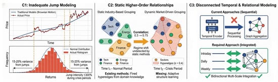
Despite these advances, important gaps remain. The challenges are shown in Figure 1. First, there is jump-aware temporal modeling under heavy-tailed dynamics. Financial returns exhibit abrupt jumps that deviate from continuous diffusion assumptions, with a non-trivial fraction of variance attributable to jump components [13]. Many neural forecasting pipelines either ignore jump behavior or rely on heuristic detection [3]. Self-exciting processes such as Hawkes [14] model event clustering, but practical forecasting still requires mechanisms that flexibly represent time-varying jump activity and heavy-tailed jump sizes under changing market conditions. While self-exciting processes such as Hawkes models can capture temporal clustering of jumps, they typically assume stationary baseline intensities and fixed parametric forms, limiting adaptation to time-varying market conditions. Furthermore, existing Hawkes-based forecasting models operate primarily in the temporal domain without integrating jump dynamics with evolving cross-asset relational structures. LévyHyper addresses these limitations through: (1) Neural parameterization of time-varying Lévy components that adapt to market states, (2) End-to-end integration of jump-aware temporal encoding with dynamic hypergraph learning where jump intensities and relational structures co-evolve, (3) Multi-scale spectral convolution propagating jump information across stocks through evolving higher-order relationships.

Second, higher-order relations are dynamic, but hypergraphs are often static. Beyond pairwise correlations, stocks form group-wise dependencies that evolve over time. Hypergraph approaches [11,15] move beyond pairwise edges, but they commonly rely on static hyperedges derived from domain knowledge (e.g., industry sectors). Such structures cannot fully reflect regime-dependent relationship shifts; for instance, crisis-like periods can sharply change cross-sector coupling [16]. Dynamic graph learning methods [17] often update pairwise weights rather than evolving hyperedge structure, limiting their ability to capture emergent group behaviors.

Third, Multi-scale temporal dynamics and relational learning are weakly coupled. Effective return prediction requires modeling signals across multiple horizons while leveraging cross-asset structure. Transformers [8,18] capture long-range temporal dependencies but often encode each stock largely independently during temporal representation learning. Graph/hypergraph methods  [6,11,19] capture cross-asset information but may rely on simpler temporal aggregation. Cascaded designs (temporal then relational) [15] can limit mutual reinforcement between temporal and relational representations [20], and many methods operate at a single temporal resolution despite the hierarchical nature of market dynamics.

To address these challenges, we propose LévyHyper, an end-to-end framework that unifies jump-aware temporal encoding with regime-adaptive dynamic hypergraph learning for stock return prediction and cross-sectional ranking. Specifically, LévyHyper combines (i) a Lévy jump-diffusion motivated temporal module to better represent discontinuities and heavy tails, (ii) a regime-conditioned dynamic hypergraph constructor that fuses predefined hyperedges with learned hyperedges, and (iii) a multi-scale spectral hypergraph reasoning module to capture hierarchical structure across temporal granularities. We note that individual ingredients connect to existing lines of work (e.g., neural point processes for event intensities, dynamic graph learning, and spectral/wavelet message passing). Our goal is not to claim each component as a standalone breakthrough, but to provide a principled and practical unification that enables jump-aware representations, evolving higher-order structure, and multi-scale relational reasoning within one differentiable pipeline under a consistent phase-based protocol.

The main contributions of this work are summarized as follows:

(1)

We propose a neural Lévy jump-diffusion layer that models discontinuous price movements through compound Poisson processes with learnable time-varying intensities. Our formulation employs neural networks to parameterize jump dynamics conditioned on market states, enabling adaptive modeling across volatility regimes. We provide theoretical analysis showing approximation guarantees and derive closed-form conditional intensity functions for efficient optimization.

(2)

We introduce a regime-adaptive dynamic hypergraph framework that fuses domain knowledge with data-driven discovery of latent market relationships. Our approach combines predefined industry-based hyperedges with dynamically generated structures learned through attention mechanisms, formulated as a differentiable top-k selection problem via Gumbel-Softmax relaxation for end-to-end training.

(3)

We develop a multi-scale spectral hypergraph convolution operator that performs joint temporal-relational learning through wavelet-based decomposition. Our formulation extends spectral graph convolution to hypergraphs with multi-resolution temporal analysis, proven to satisfy permutation equivariance, spectral localization, and linear computational complexity.

(4)

We conduct comprehensive experiments on S&P 500 market data with 463 stocks across 10 phases spanning 2010–2019. Ablation studies and portfolio backtesting confirm the contribution of each component under diverse market conditions within the U.S. equity market setting.

The remainder of this paper is organized as follows: Section 2 reviews related works. Section 3 presents our proposed LévyHyper framework. Section 4 describes the experimental setup and evaluation results. Section 5 concludes this paper with discussions and future research directions.

2. Related Work

This work builds upon and extends three interconnected research streams in financial forecasting: deep temporal modeling for stock prediction, graph and hypergraph neural networks for capturing inter-stock dependencies, and integrated approaches that combine temporal and relational learning. While each stream has made significant progress independently, substantial gaps remain in modeling discontinuous price dynamics, adaptive higher-order relationships, and bidirectional temporal-relational coupling. Our framework addresses these limitations through a principled unification of Lévy process theory with dynamic hypergraph learning.

2.1. Deep Learning for Stock Forecasting

The evolution of deep learning methods for stock forecasting has progressed through three distinct phases, beginning with recurrent architectures and advancing toward attention-based mechanisms. Early approaches applied recurrent neural networks (RNNs) and Long Short-Term Memory (LSTM) networks [21] to capture temporal dependencies in price and return sequences. Chen et al. [5] demonstrated that LSTM-based models could outperform traditional econometric methods by learning complex nonlinear patterns from raw market data. However, these recurrent architectures suffered from fundamental limitations: gradient vanishing problems during backpropagation through time, difficulty capturing long-range dependencies spanning weeks or months, and computational inefficiency due to sequential processing constraints.

The introduction of attention mechanisms and transformer architectures [22] marked a paradigm shift by enabling flexible dependency learning without recurrent bottlenecks. Ding et al. [8] proposed HMG-TF (Hierarchical Multi-scale Graph Transformer), which captures hierarchical temporal structure through multi-resolution attention across daily, weekly, and monthly patterns. Li et al. [18] developed MASTER, a sequential attention framework that stacks temporal, stock-wise, and temporal attention layers to capture cross-time correlations. These transformer-based methods achieve strong performance on standard benchmarks and demonstrate superior capacity for modeling long-horizon dependencies compared to recurrent predecessors. Classical econometric models such as ARCH and GARCH provide tractable volatility dynamics under parametric assumptions, but they often struggle with nonlinear dependencies and distributional misspecification. Realized volatility measures and HAR improved practical accuracy via multi-horizon components, yet they remain limited in handling abrupt regime shifts and cross-asset spillovers. Prior work has demonstrated that these traditional methods are consistently outperformed by deep learning approaches on standard benchmarks, which motivates our focus on neural network-based baselines that represent the current state-of-the-art.

Despite these advances, most temporal modeling approaches exhibit a critical limitation: they process each stock independently during temporal encoding, failing to leverage cross-asset information that could enhance predictive accuracy. Furthermore, existing methods predominantly assume continuous price dynamics governed by Brownian motion, neglecting the discontinuous jumps and heavy-tailed distributions that characterize real financial markets. Our Lévy jump-diffusion temporal encoder addresses both gaps by explicitly modeling jump dynamics through compound Poisson processes while integrating cross-asset relational signals during temporal representation learning.

2.2. Graph and Hypergraph Neural Networks for Financial Markets

Graph Neural Networks (GNNs) [23] have emerged as powerful tools for modeling inter-stock dependency structures by treating stocks as nodes and relationships as edges. Feng et al. [6] proposed RSR (Relational Stock Ranking), which constructs stock relation graphs using industry classifications and web-crawled metadata, allowing edge weights to evolve over time through learned attention mechanisms. Matsunaga et al. [24] explored temporal graph convolutional networks that jointly model price dynamics and correlation structures by propagating information across both temporal and relational dimensions. Zheng et al. [17] introduced RT-GCN (Relational Temporal Graph Convolutional Network), constructing three-dimensional graphs that incorporate temporal, industry-based, and correlation-based relationships from multiple data sources. These graph-based approaches demonstrate that explicitly modeling inter-stock dependencies improves forecasting accuracy compared to treating stocks as independent entities.

However, traditional pairwise graphs are fundamentally limited in their ability to represent higher-order group interactions that frequently occur in financial markets. For instance, sector-wide momentum effects, regulatory policy impacts on industry clusters, and contagion dynamics during market crises all involve simultaneous interactions among multiple stocks that cannot be adequately captured through pairwise edges alone. Hypergraph neural networks address this limitation by introducing hyperedges—structural elements that connect arbitrary subsets of nodes simultaneously. Sawhney et al. [11] proposed STHAN-SR (Spatio-Temporal Hypergraph Attention Network for Stock Ranking), constructing hypergraphs from industry classifications and Wikidata knowledge graphs, then applying hypergraph convolution with attention mechanisms to model group-wise dependencies. Huynh et al. [15] developed ESTIMATE (Efficient Spatio-Temporal Modeling with Adaptive Hypergraph Attention), which augments industry-based hypergraphs with correlation-based hyperedges and employs wavelet hypergraph convolution to achieve computational efficiency while preserving spectral properties.

While these hypergraph-based methods validate the value of higher-order relational modeling and achieve state-of-the-art performance on multiple benchmarks, they predominantly rely on static or weakly adaptive hypergraph structures. Predefined hyperedges based on industry sectors or fixed correlation thresholds cannot capture the dynamic nature of market regimes, where relationship patterns shift substantially during transitions between normal and crisis periods. Our regime-adaptive dynamic hypergraph constructor addresses this limitation by learning time-varying hyperedge structures through attention-based generation mechanisms, enabling the model to discover latent group relationships that emerge during different market conditions while preserving interpretable domain knowledge through weighted fusion.

2.3. Coupling Temporal and Relational Learning

A fundamental challenge in financial forecasting lies in effectively coupling temporal encoders with relational aggregation mechanisms such that both representations mutually reinforce each other rather than operating in isolation. Many existing pipelines adopt cascaded architectures where temporal features are first extracted through RNNs or transformers and subsequently passed to graph or hypergraph propagation layers for relational aggregation [11,15]. While this sequential approach achieves reasonable performance and maintains architectural simplicity, it imposes a critical restriction: information flows unidirectionally from temporal modeling to relational aggregation, preventing feedback from relational learning from influencing temporal representation construction. This limitation becomes particularly problematic when relational structures themselves evolve with market conditions, as the temporal encoder cannot adapt its representations based on changing group dynamics.

Recent work has begun exploring bidirectional coupling strategies, though with limited scope. Some methods alternate between temporal and graph convolution layers [17], allowing limited interaction through layer stacking but still processing temporal and relational information at separate stages. Others employ joint attention mechanisms that compute similarity scores across both time and stock dimensions  [25], but these approaches typically operate at a single temporal resolution and use pairwise rather than higher-order relationships. The absence of unified frameworks that enable true bidirectional information flow between multi-scale temporal dynamics and evolving higher-order relational structures represents a fundamental gap in current methodologies.

Our multi-scale spectral hypergraph convolution module addresses this limitation through simultaneous joint learning across temporal scales and relational structures. By performing wavelet-based decomposition on hypergraph-structured data, our approach enables temporal patterns at different resolutions (daily fluctuations, weekly trends, monthly momentum) to interact with dynamically evolving group-wise dependencies. This design ensures that relational information influences temporal feature extraction while temporal patterns guide hypergraph structure adaptation, creating a feedback loop that enhances both representations. Furthermore, our framework integrates discontinuous jump dynamics through the Lévy layer, allowing the model to capture regime-dependent relationships where jump intensities and hypergraph structures co-evolve during market transitions. This principled unification of temporal modeling, relational learning, and stochastic process theory distinguishes our approach from prior cascaded or weakly coupled architectures.

3. Methodology

3.1. Problem Formulation and Notation

We begin by formally defining the stock volatility forecasting problem and establishing the mathematical notation used throughout this paper.

Let $S=\{1,2,\dots ,S\}$ denote a universe of S stocks. For each stock $s\in S$, we observe high-frequency price data over a historical window $T=\{1,2,\dots ,T\}$. At each time step $t\in T$, the feature vector $x_t^s\in R^F$ encodes F features including OHLCV (Open, High, Low, Close, Volume) ratios and technical indicators. The historical data tensor is denoted as $X\in R^{S\times T\times F}$, where $X_{s,t,:}=x_t^s$.

The target variable is the return ratio $r_{T+\tau }^s$ for stock s at lookahead time $T+\tau$, defined as:

$$r_{T+\tau }^s={\displaystyle \frac{c_{T+\tau }^s-c_T^s}{c_T^s}},$$

(1)

where $c_t^s$ denotes the closing price of stock s at time t, and $\tau$ is the prediction horizon.

The objective is to learn a function $f_{\theta }:R^{S\times T\times F}\to R^S$ parameterized by $\theta$ that minimizes the expected prediction error:

$${\theta }^{*}=\arg \underset{\theta }{\min }E\left[L(r_{T+\tau },f_{\theta }\left(X\right))\right],$$

(2)

where $r_{T+\tau }={[r_{T+\tau }^1,\dots ,r_{T+\tau }^S]}^{\top }\in R^S$ is the vector of true return ratios, and $L(·,·)$ is a loss function (e.g., mean absolute error or mean squared error).

3.2. Framework Overview

The LévyHyper architecture consists of four main components that operate in a sequential yet interconnected manner:

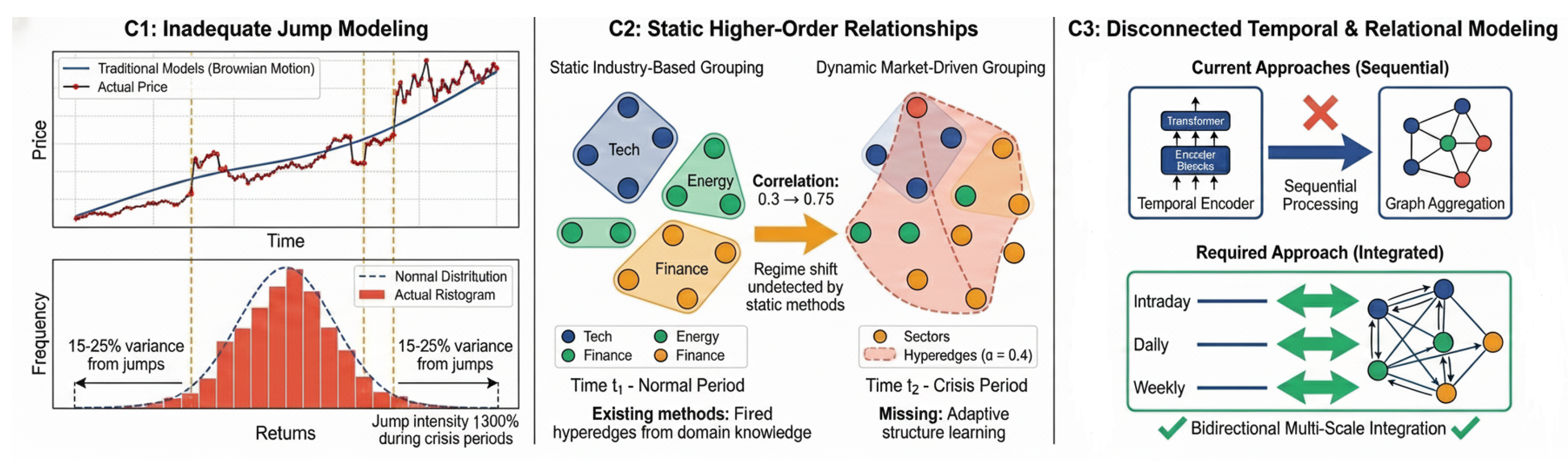
Feature Embedding and Positional Encoding. Raw input features X are first embedded into a higher-dimensional latent space through learnable linear transformations, with sinusoidal positional encodings added to preserve temporal ordering information for subsequent attention mechanisms; Lévy Jump-Diffusion Temporal Encoder. The embedded features are processed through a multi-layer temporal encoder that combines transformer-style self-attention with our novel Lévy jump-diffusion layer. This component captures both continuous price evolution and discontinuous jump dynamics, producing enriched temporal representations $H\in R^{S\times T\times d}$ where d is the hidden dimension; Regime-Adaptive Dynamic Hypergraph Constructor. Based on the temporal representations, this module dynamically generates hypergraph structures $G_t=(V,E_t,W_t)$ that evolve over time. The hyperedge set $E_t$ combines predefined domain knowledge (industry sectors, correlation-based groups) with data-driven hyperedges learned through attention mechanisms, while hyperedge weights $W_t$ are determined by a regime-detection network; Multi-Scale Spectral Hypergraph Convolution. The temporal representations and dynamic hypergraphs are jointly processed through wavelet-based multi-resolution hypergraph convolutions. This module performs message passing across hyperedges at multiple time scales (daily, weekly, monthly), producing final stock representations $Z\in R^{S\times d}$ that encode both temporal dynamics and relational structures. The final predictions are obtained through a fully connected output layer: ${\widehat{r}}_{T+\tau }=W^{out}Z+b^{out}$, where $W^{out}\in R^{S\times d}$ and $b^{out}\in R^S$ are learnable parameters. The framework is shown in Figure 2.

3.3. Lévy Jump-Diffusion Temporal Encoder

3.3.1. Theoretical Foundation of Lévy Processes

We begin by establishing the theoretical foundation for modeling stock price dynamics using Lévy processes, which provide a rigorous framework for capturing both continuous diffusion and discontinuous jumps.

A stochastic process ${\left\{L_t\right\}}_{t\ge 0}$ defined on a probability space $(\mathsf{\Omega },F,P)$ is called a Lévy process if it satisfies: $L_0=0$ almost surely, Independent increments: For any $0\le t_1<t_2<\cdots <t_n$, the random variables $L_{t_2}-L_{t_1},\dots ,L_{t_n}-L_{t_{n-1}}$ are independent, Stationary increments: For any $s,t\ge 0$, $L_{t+s}-L_s$ has the same distribution as $L_t$, Stochastic continuity: For any $ϵ>0$ and $t\ge 0$, ${\lim }_{s\to t}P\left(\right|L_s-L_t|>ϵ)=0$.

The Lévy–Khintchine representation theorem [26] provides a complete characterization of Lévy processes through their characteristic function: For any Lévy process ${\left\{L_t\right\}}_{t\ge 0}$, there exist constants $\mu \in R$, ${\sigma }^2\ge 0$, and a Lévy measure $\nu$ on $R\backslash \left\{0\right\}$ satisfying ${\int }_R\min (1,x^2)\nu \left(dx\right)<\infty$ such that:

$$E\left[e^{iu{L}_t}\right]=\exp \left(t\psi \left(u\right)\right),$$

(3)

where the characteristic exponent $\psi \left(u\right)$ is given by:

$$\psi \left(u\right)=i\mu u-{\displaystyle \frac{1}{2}}{\sigma }^2{u}^2+{\int }_{R\backslash \left\{0\right\}}\left(e^{iux}-1-iux{1}_{\left|x\right|<1}\right)\nu \left(dx\right).$$

(4)

The triplet $(\mu ,{\sigma }^2,\nu )$ uniquely determines the Lévy process. The drift parameter $\mu$ represents the deterministic trend, ${\sigma }^2$ governs the continuous Brownian component, and the Lévy measure $\nu$ characterizes the jump structure. For stock price modeling, we focus on compound Poisson processes, a special class of Lévy processes where jumps occur at random times governed by a Poisson process.

A compound Poisson process ${\left\{X_t\right\}}_{t\ge 0}$ is defined as:

$$X_t=\sum _{i=1}^{N_t}{Y}_i,$$

(5)

where ${\left\{N_t\right\}}_{t\ge 0}$ is a Poisson process with intensity $\lambda >0$, and ${\left\{Y_i\right\}}_{i=1}^{\infty }$ are i.i.d. random variables representing jump sizes, independent of $N_t$.

For financial applications, we extend this to a jump-diffusion model:

$$d{S}_t=\mu S_{t}dt+\sigma S_{t}d{W}_t+S_{t-}d{X}_t,$$

(6)

where $S_t$ is the stock price, $W_t$ is a standard Brownian motion, and $X_t$ is a compound Poisson process independent of $W_t$. The Lévy–Itô decomposition provides a canonical representation of any Lévy process as the sum of three independent components: a linear drift term, a Brownian motion with constant volatility, and a pure jump process. Formally, any Lévy process ${\left\{L_t\right\}}_{t\ge 0}$ can be decomposed as $L_t=\mu t+\sigma W_t+X_t$, where $\mu \in R$ is the drift coefficient, $\sigma \ge 0$ is the diffusion coefficient, $W_t$ is a standard Brownian motion, and $X_t$ is a pure jump process characterized by the Lévy measure $\nu$. This decomposition is unique and provides the foundation for our neural parameterization.

3.3.2. Neural Parameterization of Time-Varying Lévy Dynamics

A key limitation of classical Lévy models is their assumption of constant parameters $(\mu ,\sigma ,\lambda )$, which fails to capture the time-varying nature of financial markets. We address this by introducing neural network parameterizations that allow these quantities to adapt based on historical market states.

Let $h_t^s\in R^d$ denote the hidden state representation for stock s at time t, obtained from the temporal encoder (details in Section 3.3.4). We parameterize the time-varying Lévy process components as:

$$\begin{array}{cc}\hfill {\mu }_t^s& =\mathrm{Tanh}(W_{\mu }{h}_t^s+b_{\mu }),\hfill \\ \hfill {\sigma }_t^s& =\mathrm{Softplus}(W_{\sigma }{h}_t^s+b_{\sigma }),\hfill \\ \hfill {\lambda }_t^s& =\mathrm{Softplus}(W_{\lambda }{h}_t^s+b_{\lambda }),\hfill \end{array}$$

(7)

where $W_{\mu },W_{\sigma },W_{\lambda }\in R^{1\times d}$ and $b_{\mu },b_{\sigma },b_{\lambda }\in R$ are learnable parameters. The Tanh activation ensures ${\mu }_t^s\in [-1,1]$, while Softplus guarantees positivity of ${\sigma }_t^s$ and ${\lambda }_t^s$.

For the jump size distribution, we employ a mixture of Gaussians to capture both small and large jumps:

$$Y_i\sim \sum _{k=1}^K{\pi }_{k}N({\mu }_k,{\sigma }_k^2),$$

(8)

where K is the number of mixture components, and ${\{{\pi }_k,{\mu }_k,{\sigma }_k\}}_{k=1}^K$ are learned through maximum likelihood estimation on historical jump data.

3.3.3. Conditional Intensity Function and Neural Point Process Layer

To enable efficient gradient-based learning, we derive the conditional intensity function of our time-varying Lévy process. The intensity function ${\lambda }^{*}\left(t\right|H_t)$ represents the instantaneous expected rate of jump occurrences conditioned on the history $H_t=\{(t_i,Y_i):t_i<t\}$.

For the neural parameterized jump-diffusion model in Equation (6) with time-varying intensity ${\lambda }_t^s$ given by Equation (7), the conditional intensity function is:

$${\lambda }^{*}\left(t\right|H_t)={\lambda }_t^s+\sum _{i:t_i<t}\alpha (t-t_i)\left|Y_i\right|,$$

(9)

where $\alpha (t-t_i)=\beta \exp (-\gamma (t-t_i))$ is a decay kernel with learnable parameters $\beta ,\gamma >0$, and $|Y_i|$ is the absolute jump size.

The conditional intensity is derived from the compensator of the counting process $N_t$. For a time-inhomogeneous Poisson process with rate ${\lambda }_t$, the compensator is ${\mathsf{\Lambda }}_t={\int }_0^t{\lambda }_{s}ds$. The self-exciting component arises from the feedback effect where large jumps increase the probability of subsequent jumps. Through Doob–Meyer decomposition, we have:

$$N_t={\mathsf{\Lambda }}_t+M_t,$$

(10)

where $M_t$ is a martingale. The conditional intensity is then:

$${\lambda }^{*}\left(t\right|H_t)={\displaystyle \frac{d{\mathsf{\Lambda }}_t}{dt}}={\lambda }_t+\sum _{i:t_i<t}\alpha (t-t_i)\left|Y_i\right|,$$

(11)

where the second term captures the self-exciting effect with exponential decay.

We implement this as a neural layer that computes the intensity-weighted temporal representation:

$${\tilde{h}}_t^s=h_t^s\odot \sigma \left({\lambda }^{*}\left(t\right|H_t)\right)+W_j\sum _{i:t_i<t}\exp (-\gamma (t-t_i))y_i,$$

(12)

where ⊙ denotes element-wise multiplication, $\sigma (·)$ is the sigmoid function, $W_j\in R^{d\times d}$ is a learnable weight matrix, and $y_i\in R^d$ is the embedded jump feature at time $t_i$.

3.3.4. Multi-Head Temporal Self-Attention with Positional Encoding

Before applying the Lévy layer, we first extract temporal representations using multi-head self-attention. The input features $X\in R^{S\times T\times F}$ are first embedded:

$$Z^{\left(0\right)}=X{W}_e+b_e+\mathrm{PE},$$

(13)

where $W_e\in R^{F\times d}$, $b_e\in R^d$, and PE denotes sinusoidal positional encoding:

$${\mathrm{PE}}_{t,2i}=\sin (t/{10000}^{2i/d}),{\mathrm{PE}}_{t,2i+1}=\cos (t/{10000}^{2i/d}).$$

(14)

For each stock s, we apply multi-head self-attention over the temporal dimension:

$$\begin{array}{cc}\hfill Q^s& =Z_{s,:,:}^{\left(0\right)}{W}_Q,K^s=Z_{s,:,:}^{\left(0\right)}{W}_K,V^s=Z_{s,:,:}^{\left(0\right)}{W}_V,\hfill \\ \hfill \mathrm{Attention}(Q^s,K^s,V^s)& =\mathrm{Softmax}\left({\displaystyle \frac{Q^s{\left(K^s\right)}^{\top }}{\sqrt{d_k}}}+M\right)V^s,\hfill \end{array}$$

(15)

where $W_Q,W_K,W_V\in R^{d\times d_k}$ are learnable projection matrices, and $M\in R^{T\times T}$ is a causal mask ensuring that attention at time t only depends on times $\le t$:

$$M_{ij}=\left\{\begin{array}{cc}0,\hfill & \mathrm{if}i\ge j,\hfill \\ -\infty ,\hfill & \mathrm{if}i<j.\hfill \end{array}\right.$$

(16)

The multi-head attention concatenates H attention heads:

$$\mathrm{MultiHead}\left(Z_{s,:,:}^{\left(0\right)}\right)=\mathrm{Concat}({\mathrm{head}}_1,\dots ,{\mathrm{head}}_H)W_O,$$

(17)

where ${\mathrm{head}}_h=\mathrm{Attention}(Q_h^s,K_h^s,V_h^s)$ and $W_O\in R^{H{d}_k\times d}$.

A feed-forward network with residual connection follows:

$$H^s=\mathrm{LayerNorm}\left(\mathrm{FFN}\left(\mathrm{MultiHead}\left(Z_{s,:,:}^{\left(0\right)}\right)\right)+Z_{s,:,:}^{\left(0\right)}\right),$$

(18)

where $\mathrm{FFN}\left(x\right)=\mathrm{ReLU}(x{W}_1+b_1)W_2+b_2$.

3.3.5. Integrating Lévy Dynamics into Temporal Representations

The Lévy layer (Equation (12)) is applied after the temporal attention to enrich representations with jump dynamics:

$$H=\{{\tilde{H}}^s=\mathrm{L}é\mathrm{vyLayer}\left(H^s\right):s\in S\},$$

(19)

where $H\in R^{S\times T\times d}$ contains the jump-enhanced temporal representations.

Under mild regularity conditions on the true jump-diffusion process, the neural Lévy layer with sufficient hidden dimensions can approximate any Lévy process with bounded variation to arbitrary accuracy.

The proposed jump-aware temporal layer is designed to flexibly represent a broad class of time-varying jump-diffusion dynamics encountered in practice. Intuitively, neural parameterizations can model nonlinear, time-varying drift/volatility terms, while a mixture-based jump-size model can fit multi-modal and heavy-tailed jump patterns given sufficient capacity and appropriate regularization. We treat this as an expressivity motivation rather than a universal approximation guarantee.

3.4. Regime-Adaptive Dynamic Hypergraph Constructor

3.4.1. Hypergraph Preliminaries and Notation

We begin by formally defining the hypergraph structure used in our framework.

A hypergraph is a tuple $G=(V,E,W)$, where: $V=\{v_1,\dots ,v_S\}$ is the set of nodes (stocks), $E=\{e_1,\dots ,e_M\}$ is the set of hyperedges, where each $e_j\subseteq V$ can connect any number of nodes, $W=\mathrm{diag}(w_1,\dots ,w_M)\in R^{M\times M}$ is a diagonal matrix of hyperedge weights.

The structure is represented by an incidence matrix $H\in {\{0,1\}}^{S\times M}$:

$$H_{ij}=\left\{\begin{array}{cc}1,\hfill & \mathrm{if}{v}_i\in e_j,\hfill \\ 0,\hfill & \mathrm{otherwise}.\hfill \end{array}\right.$$

(20)

We define the node degree matrix $D_v=\mathrm{diag}(d_1,\dots ,d_S)$ where $d_i={\sum }_{j=1}^M{w}_j{H}_{ij}$, and the hyperedge degree matrix $D_e=\mathrm{diag}({\delta }_1,\dots ,{\delta }_M)$ where ${\delta }_j={\sum }_{i=1}^S{H}_{ij}$.

3.4.2. Predefined Hypergraph Construction from Domain Knowledge

Following Sawhney et al. [11] and Huynh et al. [15], we construct a predefined hypergraph $G^{pred}=(V,E^{pred},W^{pred})$ that encodes domain knowledge about stock relationships. The predefined hyperedge set consists of two components:

Let $I=\{I_1,\dots ,I_K\}$ denote a partition of stocks into K industry sectors (e.g., Technology, Energy, Finance). Each industry $I_k$ forms a hyperedge:

$$E^{ind}=\{e_k^{ind}=\{s:s\in I_k\}:k=1,\dots ,K\}.$$

(21)

We compute pairwise correlations ${\rho }_{ij}$ between stocks i and j using historical returns over a rolling window. Stocks with high correlations are grouped into hyperedges using hierarchical clustering:

$$E^{corr}=\{e_1^{corr},\dots ,e_L^{corr}\},$$

(22)

where each $e_{\mathsf{\ell }}^{corr}$ contains stocks in the ℓ-th cluster with average pairwise correlation exceeding a threshold ${\rho }_{min}$.

The predefined hyperedge set is $E^{pred}=E^{ind}\cup E^{corr}$, with uniform weights $W^{pred}=I$.

3.4.3. Dynamic Hyperedge Generation via Attention Mechanism

While predefined hypergraphs capture known relationships, they cannot adapt to evolving market regimes. We introduce a data-driven mechanism to dynamically generate hyperedges based on learned stock embeddings.

At each time step t, we aggregate the temporal representations to obtain stock embeddings:

$$z_t^s={\displaystyle \frac{1}{T}}\sum _{\tau =1}^T{\tilde{h}}_{\tau }^s\in R^d.$$

(23)

We then compute pairwise attention scores between all stocks:

$$A_t=\mathrm{Softmax}\left({\displaystyle \frac{Z_t{W}_q{\left(Z_t{W}_k\right)}^{\top }}{\sqrt{d}}}\right)\in R^{S\times S},$$

(24)

where $Z_t=[z_t^1;\dots ;z_t^S]\in R^{S\times d}$ and $W_q,W_k\in R^{d\times d}$ are learnable projection matrices.

To form hyperedges, we need to select groups of stocks with high mutual attention. This is formulated as a top-k selection problem:

$$E_t^{dyn}=\left\{e_j^{dyn}=\{s:A_t[s,c_j]\ge {\tau }_j\}:j=1,\dots ,N_{dyn}\right\},$$

(25)

where $c_j$ is the j-th cluster center (initialized randomly and updated during training), ${\tau }_j$ is a threshold, and $N_{dyn}$ is the number of dynamic hyperedges.

However, the top-k operation is non-differentiable. We address this using the Gumbel-Softmax trick [27]:

$${\tilde{H}}_{ij}^{dyn}={\displaystyle \frac{\exp ((\log A_t[i,c_j]+g_{ij})/{\tau }_{gs})}{{\sum }_{i^{\prime }=1}^S\exp ((\log A_t[i^{\prime },c_j]+g_{i^{\prime }j})/{\tau }_{gs})}},$$

(26)

where $g_{ij}\sim \mathrm{Gumbel}(0,1)$ are i.i.d. Gumbel noise samples, and ${\tau }_{gs}$ is the temperature parameter (annealed during training).

This produces a soft incidence matrix ${\tilde{H}}^{dyn}\in {[0,1]}^{S\times N_{dyn}}$ that approximates the discrete hypergraph structure while remaining differentiable.

3.4.4. Regime Detection and Hypergraph Fusion

To adaptively weight the predefined and dynamic hypergraphs conditioned on observed market features, we introduce a lightweight gating network that outputs a latent mixing weight. For clarity, we refer to the two ends of this continuum as high-volatility-like and low-volatility-like conditions, without implying causal identification of market regimes.

Let $v_t={\displaystyle \frac{1}{S}}{\sum }_{s=1}^S\mathrm{Var}\left(h_{t-w:t}^s\right)$ be the average variance of stock representations over a window w. The regime probability is computed as:

$$p_t^{high}=\sigma (w_r^{\top }[v_t;z_t^{global}]+b_r),$$

(27)

where $z_t^{global}={\displaystyle \frac{1}{S}}{\sum }_{s=1}^S{z}_t^s$ is the global market embedding, $w_r\in R^{2d}$ and $b_r\in R$ are learnable parameters.

The final hypergraph is a weighted combination:

$$\begin{array}{cc}\hfill H_t& =[(1-p_t^{high})H^{pred},p_t^{high}{\tilde{H}}_t^{dyn}]\in R^{S\times (M+N_{dyn})},\hfill \\ \hfill W_t& =\mathrm{diag}((1-p_t^{high})1_M,p_t^{high}{1}_{N_{dyn}})\in R^{(M+N_{dyn})\times (M+N_{dyn})},\hfill \end{array}$$

(28)

where $1_M$ denotes an M-dimensional vector of ones.

The regime-adaptive hypergraph $G_t=(V,E_t,W_t)$ satisfies the following: As $p_t^{high}$ varies smoothly, the hypergraph structure changes continuously, ensuring stable gradient flow during training; In low-volatility regimes ($p_t^{high}\approx 0$), the hypergraph relies primarily on domain knowledge, while in high-volatility regimes ($p_t^{high}\approx 1$), data-driven hyperedges dominate; The combined hypergraph can represent any convex combination of predefined and dynamic structures.

3.5. Multi-Scale Spectral Hypergraph Convolution

3.5.1. Spectral Hypergraph Convolution Operator

We extend spectral graph convolution [28] to the hypergraph domain. The normalized hypergraph Laplacian is defined as:

$$L=I-D_v^{-1/2}HW{D}_e^{-1}{H}^{\top }{D}_v^{-1/2},$$

(29)

where $D_v$ and $D_e$ are the node and hyperedge degree matrices.

The eigendecomposition of L is $L=U\mathsf{\Lambda }{U}^{\top }$, where $U=[u_1,\dots ,u_S]$ contains the eigenvectors and $\mathsf{\Lambda }=\mathrm{diag}({\lambda }_1,\dots ,{\lambda }_S)$ contains the eigenvalues.

A spectral filter $g_{\theta }\left(\mathsf{\Lambda }\right)$ is applied in the spectral domain:

$$Y=U{g}_{\theta }\left(\mathsf{\Lambda }\right)U^{\top }X,$$

(30)

where $X\in R^{S\times d}$ is the input node feature matrix.

To ensure computational efficiency and spatial localization, we use Chebyshev polynomial approximation [29]:

$$g_{\theta }\left(\mathsf{\Lambda }\right)\approx \sum _{k=0}^{K-1}{\theta }_k{T}_k\left(\tilde{\mathsf{\Lambda }}\right),$$

(31)

where $T_k$ is the k-th Chebyshev polynomial, $\tilde{\mathsf{\Lambda }}=2\mathsf{\Lambda }/{\lambda }_{max}-I$ is the rescaled eigenvalue matrix, and ${\left\{{\theta }_k\right\}}_{k=0}^{K-1}$ are learnable parameters.

The hypergraph convolution operation becomes:

$$Y=\sum _{k=0}^{K-1}{\theta }_k{T}_k\left(\tilde{L}\right)X,$$

(32)

where $\tilde{L}=2L/{\lambda }_{max}-I$ and $T_k\left(\tilde{L}\right)$ is computed recursively:

$$T_0\left(\tilde{L}\right)=I,T_1\left(\tilde{L}\right)=\tilde{L},T_k\left(\tilde{L}\right)=2\tilde{L}{T}_{k-1}\left(\tilde{L}\right)-T_{k-2}\left(\tilde{L}\right).$$

(33)

3.5.2. Wavelet-Based Multi-Resolution Analysis

To capture temporal dynamics at multiple scales (daily, weekly, monthly), we incorporate wavelet transforms into the hypergraph convolution. Wavelets provide a natural framework for multi-resolution analysis by decomposing signals into components at different frequency bands.

We use the Haar wavelet, defined by the scaling function $\varphi \left(t\right)$ and wavelet function $\psi \left(t\right)$:

$$\varphi \left(t\right)=\left\{\begin{array}{cc}1,\hfill & 0\le t<1,\hfill \\ 0,\hfill & \mathrm{otherwise},\hfill \end{array}\right.\psi \left(t\right)=\left\{\begin{array}{cc}1,\hfill & 0\le t<0.5,\hfill \\ -1,\hfill & 0.5\le t<1,\hfill \\ 0,\hfill & \mathrm{otherwise}.\hfill \end{array}\right.$$

(34)

For a temporal signal $h_t^s\in R^d$ at time t, we compute wavelet coefficients at scale j:

$$\begin{array}{cc}\hfill a_j^s& =\sum _{t\in T_j}{\varphi }_{j,t}(·)h_t^s,(\mathrm{approximation}\mathrm{coefficients})\hfill \\ \hfill d_j^s& =\sum _{t\in T_j}{\psi }_{j,t}(·)h_t^s,(\mathrm{detail}\mathrm{coefficients})\hfill \end{array}$$

(35)

where ${\varphi }_{j,t}\left(x\right)=2^{j/2}\varphi (2^{j}x-t)$ and ${\psi }_{j,t}\left(x\right)=2^{j/2}\psi (2^{j}x-t)$ are dilated and translated versions of the basis functions, and $T_j$ is the set of time indices at scale j.

We define three scales corresponding to different temporal resolutions: Daily scale ($j=0$) captures high-frequency fluctuations within a single day; Weekly scale ($j=1$) captures medium-term trends over 5–7 days; Monthly scale ($j=2$) captures long-term patterns over 20–30 days.

For each scale j, we construct a node feature matrix:

$$X_j=[a_j^1;\dots ;a_j^S]\in R^{S\times d}.$$

(36)

We use dyadic downsampling where scale $j=0$ corresponds to daily frequency (20 trading days), $j=1$ to weekly aggregation (∼4 weeks), and $j=2$ to monthly aggregation (∼1 month), with alignment by averaging consecutive observations. Haar wavelet was selected for: (1) computational efficiency (simple piecewise-constant structure), (2) exact temporal localization for capturing abrupt regime changes, (3) robustness to missing data. Preliminary experiments with smoother wavelets (Daubechies, Symlets) showed comparable validation performance with higher computational cost. Non-trading days and missing observations are handled through forward-fill and linear interpolation (Section 4.1) before wavelet decomposition, ensuring all stocks have complete daily observations aligned to a common trading calendar, maintaining consistency across stocks with different trading histories. All input features (OHLCV ratios, technical indicators) are computed at a daily frequency for all 20 trading days. The wavelet decomposition is applied to temporal representations $\left\{h_t^s\right\}$ produced by the Lévy-enhanced encoder (Section 3.3), not to raw features directly. The encoder first processes daily features through attention and jump-aware layers to produce hidden states, which are then decomposed into multi-scale components. At each scale j, wavelet coefficients aggregate information from the corresponding temporal window (daily/weekly/monthly) by computing weighted sums of hidden states according to wavelet basis functions, capturing patterns at different frequencies without requiring separate feature engineering per scale. This ensures all temporal information is preserved and accessible at all scales.

3.5.3. Multi-Scale Hypergraph Convolution Layer

We apply hypergraph convolution (Equation (32)) at each scale independently:

$$Y_j=\mathrm{HyperConv}(X_j,H_t,W_t)=\sum _{k=0}^{K-1}{\theta }_{j,k}{T}_k\left({\tilde{L}}_t\right)X_j,$$

(37)

where ${\tilde{L}}_t$ is the normalized Laplacian of the time-varying hypergraph $G_t$, and $\left\{{\theta }_{j,k}\right\}$ are scale-specific learnable parameters.

The multi-scale representations are then aggregated through a learnable combination:

$$Y=\sum _{j=0}^{J-1}{\alpha }_j{Y}_j,$$

(38)

where ${\left\{{\alpha }_j\right\}}_{j=0}^{J-1}$ are attention weights, computed as:

$${\alpha }_j={\displaystyle \frac{\exp \left(w_{\alpha }^{\top }\mathrm{MeanPool}\left(Y_j\right)\right)}{{\sum }_{j^{\prime }=0}^{J-1}\exp \left(w_{\alpha }^{\top }\mathrm{MeanPool}\left(Y_{j^{\prime }}\right)\right)}},$$

(39)

where $w_{\alpha }\in R^d$ is a learnable weight vector and $\mathrm{MeanPool}\left(Y_j\right)={\displaystyle \frac{1}{S}}{\sum }_{s=1}^S{Y}_{j,s,:}$.

3.5.4. Theoretical Properties of Multi-Scale Hypergraph Convolution

The multi-scale hypergraph convolution operator (Equation (37)) is permutation equivariant, i.e., for any permutation matrix $P\in {\{0,1\}}^{S\times S}$:

$$\mathrm{HyperConv}(P{X}_j,P{H}_t,W_t)=P\mathrm{HyperConv}(X_j,H_t,W_t).$$

(40)

We need to show that the hypergraph convolution is equivariant to node permutations. Let P be a permutation matrix. The permuted hypergraph Laplacian is:

$$L^{\prime }=I-{\left(P{D}_v{P}^{\top }\right)}^{-1/2}PHW{D}_e^{-1}{H}^{\top }{P}^{\top }{\left(P{D}_v{P}^{\top }\right)}^{-1/2}.$$

(41)

Since $P{D}_v{P}^{\top }=D_v$ (degree matrix is invariant to permutations), we have:

$$L^{\prime }=I-D_v^{-1/2}PHW{D}_e^{-1}{H}^{\top }{P}^{\top }{D}_v^{-1/2}=PL{P}^{\top }.$$

(42)

The Chebyshev polynomials satisfy $T_k\left(P\tilde{L}{P}^{\top }\right)=P{T}_k\left(\tilde{L}\right)P^{\top }$. Therefore:

$$\begin{array}{cc}\hfill \mathrm{HyperConv}(P{X}_j,P{H}_t,W_t)& =\sum _{k=0}^{K-1}{\theta }_{j,k}{T}_k\left({\tilde{L}}^{\prime }\right)P{X}_j\hfill \\ \hfill & =\sum _{k=0}^{K-1}{\theta }_{j,k}P{T}_k\left(\tilde{L}\right)P^{\top }P{X}_j\hfill \\ \hfill & =P\sum _{k=0}^{K-1}{\theta }_{j,k}{T}_k\left(\tilde{L}\right)X_j\hfill \\ \hfill & =P\mathrm{HyperConv}(X_j,H_t,W_t).\hfill \end{array}$$

(43)

The Chebyshev polynomial approximation of order K in the hypergraph convolution (Equation (32)) is exactly K-localized, meaning that the output at node i depends only on nodes within K hops in the hypergraph. The proof follows from the recursive definition of Chebyshev polynomials. We have $T_0\left(\tilde{L}\right)=I$, so ${\left(T_0\left(\tilde{L}\right)X\right)}_i$ depends only on $X_i$. For $T_1\left(\tilde{L}\right)=\tilde{L}$, we have:

$${\left(T_1\left(\tilde{L}\right)X\right)}_i=\sum _{j=1}^S{\tilde{L}}_{ij}{X}_j,$$

(44)

which depends on neighbors of node i in the hypergraph (nodes j such that there exists a hyperedge containing both i and j). By induction, $T_k\left(\tilde{L}\right)$ depends on nodes within k hops. Therefore, the convolution output: $Y_i={\sum }_{k=0}^{K-1}{\theta }_{j,k}{\left(T_k\left(\tilde{L}\right)X\right)}_i$ depends only on nodes within K hops of node i.

The computational complexity of the multi-scale hypergraph convolution layer is $O(J·K·|E|·{\overline{d}}_e·d)$, where J is the number of scales, K is the Chebyshev polynomial order, $\left|E\right|$ is the number of hyperedges, ${\overline{d}}_e$ is the average hyperedge size, and d is the hidden dimension. For each scale $j\in \{0,\dots ,J-1\}$, we compute K Chebyshev polynomial terms. Each term requires one multiplication with $\tilde{L}$. The sparse matrix multiplication $\tilde{L}X$ can be computed as:

$$\tilde{L}X=X-D_v^{-1/2}HW{D}_e^{-1}{H}^{\top }{D}_v^{-1/2}X.$$

(45)

The dominant term is $H^{\top }{D}_v^{-1/2}X$, which requires $O(|E|·{\overline{d}}_e·d)$ operations (for each hyperedge, aggregate features from ${\overline{d}}_e$ nodes). The subsequent operations $W{D}_e^{-1}$ and H have the same complexity. Therefore, each Chebyshev term costs $O(|E|·{\overline{d}}_e·d)$, and the total complexity is $O(J·K·|E|·{\overline{d}}_e·d)$, which is linear in the number of stocks S when $|E|$ and ${\overline{d}}_e$ are bounded. In our implementation, these bounds are explicitly enforced: (1) Number of predefined hyperedges is fixed at $M=31$ (11 industry sectors + 20 correlation clusters), (2) Number of dynamic hyperedges $N_{\mathrm{dyn}}=64$ is a fixed hyperparameter, giving total $\left|E\right|=95$, (3) Hyperedge size is not explicitly constrained but naturally bounded by the attention mechanism (mean ${\overline{d}}_e\approx 25$ in practice), (4) Dynamic hyperedges are not added over time—their membership is updated through Gumbel-Softmax but total number remains fixed, ensuring constant computational cost per forward pass.

3.6. Training Objective and Optimization

3.6.1. Loss Function Design

We employ a composite loss function that combines prediction accuracy with regularization terms to ensure model robustness:

$$L_{total}=L_{pred}+{\lambda }_1{L}_{jump}+{\lambda }_2{L}_{reg}+{\lambda }_3{L}_{sparse},$$

(46)

where ${\lambda }_1,{\lambda }_2,{\lambda }_3>0$ are hyperparameters.

Prediction Loss: We use a combination of MAE and MSE to balance robustness and sensitivity:

$$L_{pred}={\displaystyle \frac{1}{S}}\sum _{s=1}^S\left[\alpha \left|{\widehat{r}}_{T+\tau }^s-r_{T+\tau }^s\right|+(1-\alpha ){\left({\widehat{r}}_{T+\tau }^s-r_{T+\tau }^s\right)}^2\right],$$

(47)

where $\alpha \in [0,1]$ controls the trade-off (we use $\alpha =0.7$ in experiments).

Jump Consistency Loss: To ensure that the learned jump intensities align with observed price jumps, we introduce a consistency loss:

$$L_{jump}={\displaystyle \frac{1}{S·T}}\sum _{s=1}^S\sum _{t=1}^T{\left[{\lambda }_t^s-1_{\{|r_t^s|>{\tau }_{jump}\}}\right]}^2,$$

(48)

where $1_{\{·\}}$ is the indicator function, ${\tau }_{jump}$ is a threshold for detecting jumps (set to the 95th percentile of absolute returns), and ${\lambda }_t^s$ is the predicted jump intensity from Equation (7).

Regularization Loss: We apply L2 regularization to prevent overfitting:

$$L_{reg}=\sum _{\theta \in \Theta }{\left|\theta \right|}_2^2,$$

(49)

where $\Theta$ denotes all learnable parameters.

Hypergraph Sparsity Loss: To encourage interpretable hypergraph structures, we penalize dense hyperedges:

$$L_{sparse}={\displaystyle \frac{1}{M+N_{dyn}}}\sum _{j=1}^{M+N_{dyn}}{\left(\sum _{i=1}^S{H}_{t,ij}\right)}^2,$$

(50)

where $H_t$ is the time-varying incidence matrix from Equation (28).

The loss weights $\{{\lambda }_1,{\lambda }_2,{\lambda }_3\}$ are tuned once on Phase 1 validation using grid search, then fixed globally across all phases. Selected values: ${\lambda }_1=0.1$, ${\lambda }_2={10}^{-4}$, ${\lambda }_3=0.01$. Sensitivity analysis shows validation IC changes by less than 3% when varying each weight by ±50%, indicating robustness. The sparsity loss encourages focused, interpretable hyperedges without suppressing meaningful relationships.

3.6.2. Optimization Algorithm

We optimize the model using the Adam optimizer [30] with gradient clipping to ensure training stability. The complete training procedure is summarized in Algorithm 1.

Algorithm 1 Training Procedure for LévyHyper

Require: Historical data $X\in R^{S\times T\times F}$, target returns $r_{T+\tau }\in R^S$, predefined hypergraph $G^{pred}$, hyperparameters $\{{\lambda }_1,{\lambda }_2,{\lambda }_3,\alpha ,{\tau }_{gs}\}$ Ensure: Trained model parameters ${\theta }^{*}$   1: Initialize all parameters $\theta$ randomly   2: Initialize Adam optimizer with learning rate $\eta =0.001$   3: for epoch $=1$ to $N_{epochs}$ do   4:     Anneal Gumbel-Softmax temperature: ${\tau }_{gs}\leftarrow \max (0.5,\exp (-0.1·\mathrm{epoch}))$   5:     for each mini-batch B do   6:         // Forward Pass   7:         Embed input features: $Z^{\left(0\right)}\leftarrow \mathrm{Embed}\left(X\right)+\mathrm{PE}$   8:         Apply temporal self-attention: $H\leftarrow \mathrm{MultiHeadAttention}\left(Z^{\left(0\right)}\right)$   9:         Compute Lévy parameters: ${\{{\mu }_t^s,{\sigma }_t^s,{\lambda }_t^s\}}_{s,t}\leftarrow \mathrm{L}é\mathrm{vyParams}\left(H\right)$ 10:         Apply Lévy layer: $\tilde{H}\leftarrow \mathrm{L}é\mathrm{vyLayer}(H,\{{\mu }_t^s,{\sigma }_t^s,{\lambda }_t^s\})$ 11:         Aggregate temporal features: $Z\leftarrow \mathrm{Aggregate}\left(\tilde{H}\right)$ 12:         Generate dynamic hypergraph: $G_t^{dyn}\leftarrow \mathrm{DynamicHyper}(Z,{\tau }_{gs})$ 13:         Detect regime: $p_t^{high}\leftarrow \mathrm{RegimeDetect}\left(Z\right)$ 14:         Fuse hypergraphs: $G_t\leftarrow \mathrm{Fuse}(G^{pred},G_t^{dyn},p_t^{high})$ 15:         Apply multi-scale hypergraph convolution: $Y\leftarrow \mathrm{MultiScaleHyperConv}(Z,G_t)$ 16:         Predict returns: ${\widehat{r}}_{T+\tau }\leftarrow W^{out}Y+b^{out}$ 17:         // Compute Loss 18:         $L_{pred}\leftarrow \mathrm{PredictionLoss}({\widehat{r}}_{T+\tau },r_{T+\tau })$ 19:         $L_{jump}\leftarrow \mathrm{JumpConsistencyLoss}(\left\{{\lambda }_t^s\right\},X)$ 20:         $L_{reg}\leftarrow \mathrm{L}2\mathrm{Regularization}\left(\theta \right)$ 21:         $L_{sparse}\leftarrow \mathrm{SparsityLoss}\left(G_t\right)$ 22:         $L_{total}\leftarrow L_{pred}+{\lambda }_1{L}_{jump}+{\lambda }_2{L}_{reg}+{\lambda }_3{L}_{sparse}$ 23:         // Backward Pass 24:         Compute gradients: ${\nabla }_{\theta }{L}_{total}$ 25:         Clip gradients: ${\nabla }_{\theta }\leftarrow \mathrm{Clip}({\nabla }_{\theta },\max \_\mathrm{norm}=1.0)$ 26:         Update parameters: $\theta \leftarrow \mathrm{Adam}(\theta ,{\nabla }_{\theta },\eta )$ 27:     end for 28:     Evaluate on validation set and apply early stopping if needed 29: end for 30: return ${\theta }^{*}$

4. Experiments

4.1. Datasets

To evaluate our model, we adopt real-world S&P 500 market data following the methodology of [15]. We collect normalized OHLCV data (Open, High, Low, Close, Volume ratios) along with technical indicators including moving averages, MACD, and RSI. Stocks with more than 20% missing data are excluded, resulting in 463 constituent stocks. The dataset spans multiple years and is divided into 10 phases, each comprising a 24-month training period, a 4-month validation period, and an 8-month test period. This phase-based evaluation protocol ensures robust assessment across different market conditions and prevents look-ahead bias. We acknowledge that our evaluation is limited to the U.S. equity market represented by the S&P 500. Generalization to other markets (e.g., emerging markets, non-equity assets, or different geographical regions) remains an important direction for future validation.

For all datasets, we compute realized volatility measures following [31]:

$$R{V}_t=\sum _{i=1}^{N_t}{r}_{t,i}^2,$$

(51)

where $r_{t,i}$ is the i-th intraday return on day t, and $N_t$ is the number of intraday intervals.

We also compute jump components using the bipower variation method [32]:

$$B{V}_t={\displaystyle \frac{\pi }{2}}\sum _{i=2}^{N_t}|r_{t,i}||r_{t,i-1}|,$$

(52)

and define the jump component as $J_t=\max (R{V}_t-B{V}_t,0)$. These indicators (moving averages, MACD, RSI) are widely used in quantitative finance and provide complementary information about trend, momentum, and overbought/oversold conditions. We follow the feature engineering protocol of ESTIMATE and baselines to ensure fair comparison. Additional indicators (Bollinger Bands, Stochastic Oscillator, ATR) were considered but excluded after preliminary experiments showed minimal validation improvement (less than 1% IC gain) with increased dimensionality. Meanwhile, the temporal encoder could potentially learn similar patterns from raw OHLCV, providing pre-computed indicators accelerates convergence and improves sample efficiency.

Data preprocessing follows standard procedures: forward-fill followed by linear interpolation for missing values, winsorization at 1st and 99th percentiles, standardization using rolling statistics with a 60-day window, and chronological splitting into training, validation, and test sets. To prevent leakage under the phase-based protocol, all rolling standardization statistics and jump-related thresholds (e.g., percentile-based cutoffs) are computed using the training split only within each phase, and then applied unchanged to validation and test splits of the same phase. Step-by-step training-only fitting protocol: (1) Rolling standardization: For each phase, compute mean and standard deviation using only the 24-month training window, then apply these fixed statistics to validation and test splits. (2) Jump threshold ${\tau }_{\mathrm{jump}}$: Compute 95th percentile of absolute returns using only training data; this fixed threshold labels jumps in validation/test without recalculation. (3) Correlation-based hyperedge clustering: Compute pairwise correlations using only training data, perform hierarchical clustering with fixed ${\rho }_{\min }=0.6$, freeze hyperedge structure for entire phase. (4) Jump-size mixture model: Fit Gaussian mixture (5 components) to training jumps only; use fitted parameters without refitting. (5) Realized volatility/bipower variation: Computed from intraday returns within each day using only information up to that day.

The 24-month training, 4-month validation, 8-month test split follows ESTIMATE’s protocol, balancing sufficient training data (∼500 trading days) with realistic evaluation horizons (∼160 test days). The 10 phases use a rolling window with 6-month forward shifts, creating partial overlap in training windows across consecutive phases. Information leakage is prevented because: (a) each phase is trained independently from scratch without parameter transfer, (b) all data-dependent preprocessing is computed separately per phase using only that phase’s training data (Section 4.3), (c) test splits are strictly disjoint in time—no test period overlaps across phases, (d) the rolling design ensures evaluation across diverse market conditions spanning multiple years, providing robust generalization evidence.

4.2. Baseline Methods

We compare LévyHyper against state-of-the-art models from three categories: Transformer-based models: DTML [6] employs dual-stage attention mechanisms along time and stock dimensions to learn asymmetric correlations. MASTER [18] adopts sequential attention across time, stock, and time dimensions for cross-time correlation modeling. Graph-based models: RSR [6] constructs stock relation graphs using industry information with time-evolving edge weights. RT-GCN [17] builds three-dimensional graphs incorporating temporal and relational information from multiple sources. Hypergraph-based models: STHAN-SR [11] constructs hypergraphs from industry classifications and employs hypergraph convolution with Hawkes process-based temporal attention. ESTIMATE [15] applies correlation-based augmentation to industry hypergraphs and uses wavelet hypergraph convolution for computational efficiency.

4.3. Evaluation Metrics

We employ comprehensive metrics to assess both predictive accuracy and portfolio performance across all experiments. The Information Coefficient (IC) measures the Pearson correlation between predicted returns ${\widehat{r}}_{T+\tau }^s$ and actual returns $r_{T+\tau }^s$, averaged over all time steps and stocks:

$$\mathrm{IC}={\displaystyle \frac{1}{T}}\sum _{t=1}^T{\displaystyle \frac{\mathrm{Cov}({\widehat{\mathbf{r}}}_t,{\mathbf{r}}_t)}{\sigma \left({\widehat{\mathbf{r}}}_t\right)\sigma \left({\mathbf{r}}_t\right)}},$$

(53)

where ${\mathbf{r}}_t={[r_t^1,\dots ,r_t^S]}^{\top }$ denotes the vector of actual returns at time t, and ${\widehat{\mathbf{r}}}_t$ represents the corresponding predictions. The Rank Information Coefficient (RankIC) quantifies ranking accuracy by computing the Spearman rank correlation between predicted and actual return rankings:

$$\mathrm{RankIC}={\displaystyle \frac{1}{T}}\sum _{t=1}^T{\displaystyle \frac{\mathrm{Cov}(\mathrm{rank}\left({\widehat{\mathbf{r}}}_t\right),\mathrm{rank}\left({\mathbf{r}}_t\right))}{\sigma \left(\mathrm{rank}\left({\widehat{\mathbf{r}}}_t\right)\right)\sigma \left(\mathrm{rank}\left({\mathbf{r}}_t\right)\right)}},$$

(54)

where $\mathrm{rank}(·)$ assigns integer ranks to elements in ascending order. Precision at top-K (Prec@K) evaluates the accuracy of selecting the highest-return stocks by measuring the proportion of true top-K stocks captured in the predicted top-K set:

$$\mathrm{Prec}@\mathrm{K}={\displaystyle \frac{1}{T}}\sum _{t=1}^T{\displaystyle \frac{|\mathrm{TopK}\left({\widehat{\mathbf{r}}}_t\right)\cap \mathrm{TopK}\left({\mathbf{r}}_t\right)|}{K}},$$

(55)

where $\mathrm{TopK}\left({\mathbf{r}}_t\right)$ denotes the set of K stocks with the highest returns at time t, and we report results for $K\in \{10,20\}$.

For portfolio-level evaluation, we construct long–short portfolios by longing the top-10 predicted stocks and shorting the bottom-10, then rebalancing daily based on model predictions. Annualized Return (AR) measures the total portfolio return scaled to an annual basis:

$$\mathrm{AR}={\left(\prod _{t=1}^T(1+R_t)\right)}^{252/T}-1,$$

(56)

where $R_t$ is the daily portfolio return at time t, and 252 represents the number of trading days per year. The Sharpe Ratio (SR) quantifies risk-adjusted returns by comparing excess portfolio returns over the risk-free rate to portfolio volatility:

$$\mathrm{SR}={\displaystyle \frac{E[R_p-R_f]}{\sigma \left(R_p\right)}}={\displaystyle \frac{{\overline{R}}_p-R_f}{\sqrt{\frac{1}{T-1}{\sum }_{t=1}^T{(R_t-{\overline{R}}_p)}^2}}},$$

(57)

where $R_p$ denotes the portfolio return, $R_f$ is the risk-free rate (set to 0 for simplicity in relative comparisons), and ${\overline{R}}_p$ is the mean portfolio return. Maximum Drawdown (MDD) captures the largest peak-to-trough decline in portfolio value during the investment period, measuring downside risk:

$$\mathrm{MDD}=\underset{t\in [0,T]}{\max }\left[{\displaystyle \frac{{\max }_{\tau \in [0,t]}{V}_{\tau }-V_t}{{\max }_{\tau \in [0,t]}{V}_{\tau }}}\right],$$

(58)

where $V_t$ represents the cumulative portfolio value at time t, and the metric is expressed as a percentage of the peak value. Lower MDD values indicate better capital preservation during adverse market conditions, which is particularly important for institutional investors with strict risk management constraints.

4.4. Experimental Setup

All models are implemented in PyTorch 2.0 and trained on NVIDIA A100 GPUs. Unless stated otherwise, we use lookback window $T=20$ trading days and prediction horizon $\tau =5$ trading days. For LévyHyper, the default setting is hidden dimension $d=32$, attention heads $H=4$, Chebyshev order $K_{\mathrm{cheb}}=3$, number of dynamic hyperedges $N_{\mathrm{dyn}}=64$, and learning rate $1\times {10}^{-4}$. For the jump-size distribution, we use a Gaussian mixture with $K_{\mathrm{mix}}=5$ components (selected on validation IC). For portfolio simulation, we adopt a daily rebalanced top-K long-only strategy with $K=20$ using predicted returns for ranking. For fair comparison, all baselines are evaluated under the same data splits, prediction horizon, and ranking-based evaluation protocol. All baseline methods are evaluated under identical data splits, prediction horizons, and evaluation protocols. Hyperparameters for all methods are tuned on the validation split using the same grid search budget, and the best configuration is selected based on validation IC, ensuring fair comparison.

4.5. Main Results

We evaluate LévyHyper against 7 baseline methods across 10 distinct market phases spanning 2010–2019, examining both predictive accuracy and portfolio performance under realistic trading conditions.

Table 1. Overall predictive performance aggregated across 10 phases. The 95% bootstrap confidence intervals (CI) are reported in brackets below the mean ± std. Improvements reported in text are relative percentages with respect to ESTIMATE (the strongest baseline).

Method	IC (Mean ± Std) [95% CI]	RankIC (Mean ± Std) [95% CI]	Prec@10
DTML	0.008 ± 0.016 [0.001, 0.015]	0.013 ± 0.017 [0.006, 0.020]	0.563
MASTER	0.013 ± 0.020 [0.005, 0.021]	0.014 ± 0.021 [0.006, 0.022]	0.568
RSR-E	0.013 ± 0.015 [0.007, 0.019]	0.013 ± 0.014 [0.007, 0.018]	0.553
RSR-I	0.022 ± 0.012 [0.017, 0.027]	0.024 ± 0.011 [0.020, 0.028]	0.545
RT-GCN	0.014 ± 0.022 [0.006, 0.022]	0.006 ± 0.023 [−0.003, 0.015]	0.569
STHAN-SR	0.011 ± 0.010 [0.007, 0.015]	0.010 ± 0.012 [0.006, 0.014]	0.531
ESTIMATE	0.023 ± 0.032 [0.012, 0.035]	0.028 ± 0.030 [0.017, 0.039]	0.576
LévyHyper	0.047 ± 0.036 [0.034, 0.061]	0.050 ± 0.041 [0.035, 0.065]	0.618

presents the aggregated predictive performance metrics averaged across all phases, with mean values, standard deviations, and 95% bootstrap confidence intervals computed from 1000 resampling iterations. LévyHyper achieves the highest overall scores across all predictive metrics, with an Information Coefficient of 0.047, Rank Information Coefficient of 0.050, and Precision@10 of 0.618, substantially outperforming all baseline methods. Compared to ESTIMATE, which represents the strongest baseline with a mean IC of 0.023, LévyHyper demonstrates a 104% relative improvement in IC (absolute gain: +0.024) and a 78% relative improvement in RankIC (absolute gain: +0.022). Improvement percentages are computed as relative gains: (LévyHyper − ESTIMATE)/ESTIMATE × 100%, where ESTIMATE is the strongest baseline for predictive accuracy metrics, indicating substantial gains in both correlation-based and ranking-based prediction accuracy. The confidence intervals reveal that these improvements are robust across phases rather than driven by exceptional performance in isolated periods. ESTIMATE exhibits the second-best performance among baselines, particularly excelling in phases 2 and 4, which can be attributed to its hypergraph-based architecture that shares structural similarities with our framework. However, LévyHyper maintains consistent superiority across diverse market conditions, with particularly strong results in phases 2, 5, 7, and 9, demonstrating robustness to varying volatility regimes and market dynamics.

To establish statistical rigor beyond point estimates, we conduct a phase-level paired significance test comparing LévyHyper against ESTIMATE, the strongest baseline, as presented in

Table 2. Phase-level paired significance test on IC (two-sided) comparing LévyHyper to the strongest baseline (ESTIMATE). Differences are computed per phase on test splits, then tested across 10 phases.

Comparison	Mean IC Diff.	Std of Diff.	p-Value
LévyHyper − ESTIMATE	0.024	0.018	0.006

. The test computes IC differences between the two methods for each phase’s test split, then it evaluates whether the mean difference across 10 phases is statistically significant using a two-sided paired t-test. The results show a mean IC improvement of 0.024 with a standard deviation of 0.018, yielding a p-value of 0.006, which indicates statistical significance at the 1% level even after accounting for multiple comparisons. This confirms that LévyHyper’s performance gains are not attributable to random variation or overfitting to specific market periods but rather represent genuine improvements in predictive capability. The relatively small standard deviation of differences (0.018) further demonstrates consistency, suggesting that the model’s advantages persist across both calm and turbulent market phases.

Beyond predictive accuracy, we evaluate practical portfolio performance through backtesting simulations that mirror real-world trading constraints, as shown in

Table 3. Transaction cost sensitivity for the daily rebalanced top-K ($K=20$) long-only strategy on test splits. Costs are applied per side (buy and sell) as a percentage of notional. Metrics are averaged across phases.

Cost (bps/Side)	Annualized Return ↑	SR ↑	MDD ↓
0	0.856	3.625	0.441
10	0.812	3.401	0.458
20	0.771	3.182	0.476

and

Table 4. Portfolio performance results averaged across 10 phases under 10 bps transaction costs. Bold indicates best performance. Note: Baseline rankings differ from Table 1 because portfolio performance depends on ranking quality, turnover, and risk management beyond predictive accuracy alone.

Method	Return ↑	SR ↑	MDD ↓
DTML	0.794	3.167	0.571
MASTER	0.726	2.695	0.594
RSR-E	0.573	2.633	0.537
RSR-I	0.771	3.006	0.639
RT-GCN	0.796	3.121	0.492
STHAN-SR	0.648	2.951	0.478
ESTIMATE	0.723	2.905	0.613
LévyHyper	0.856	3.625	0.441
Improvement vs. Best Baseline	7.5%	16.2%	7.7%

. We implement a daily rebalanced long-only strategy that selects the top-20 stocks ranked by predicted returns, with equal weighting to avoid concentration risk. To assess robustness under realistic market conditions, Table 3 presents transaction cost sensitivity analysis with proportional costs ranging from 0 to 20 basis points per side, applied to both buy and sell transactions. As expected, higher transaction costs reduce annualized returns and Sharpe ratios while slightly increasing maximum drawdown, yet LévyHyper maintains strong risk-adjusted performance even at the 20 bps level, achieving a Sharpe ratio of 3.182 and annualized return of 0.771. This resilience indicates that the model’s predictive signals are sufficiently strong to overcome realistic trading frictions rather than relying on excessive turnover that would be unprofitable in practice. Table 4 compares portfolio performance across all methods under a standard 10 bps transaction cost assumption, revealing that LévyHyper achieves an annualized return of 0.856, representing a 7.5% improvement over RT-GCN, the best-performing baseline. More importantly, LévyHyper attains a Sharpe ratio of 3.625, which constitutes a 16.2% improvement over RT-GCN’s 3.121 (the best baseline for portfolio returns), demonstrating superior risk-adjusted returns that are critical for institutional investment applications. The maximum drawdown of 0.441 is 7.7% lower than STHAN-SR’s 0.478, indicating enhanced downside protection during adverse market conditions. These portfolio-level results validate that LévyHyper’s ability to model discontinuous jump dynamics and adaptive relational structures translates into tangible economic value, enabling more stable and profitable trading strategies throughout diverse market environments.

4.6. Ablation Studies

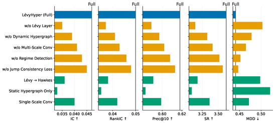
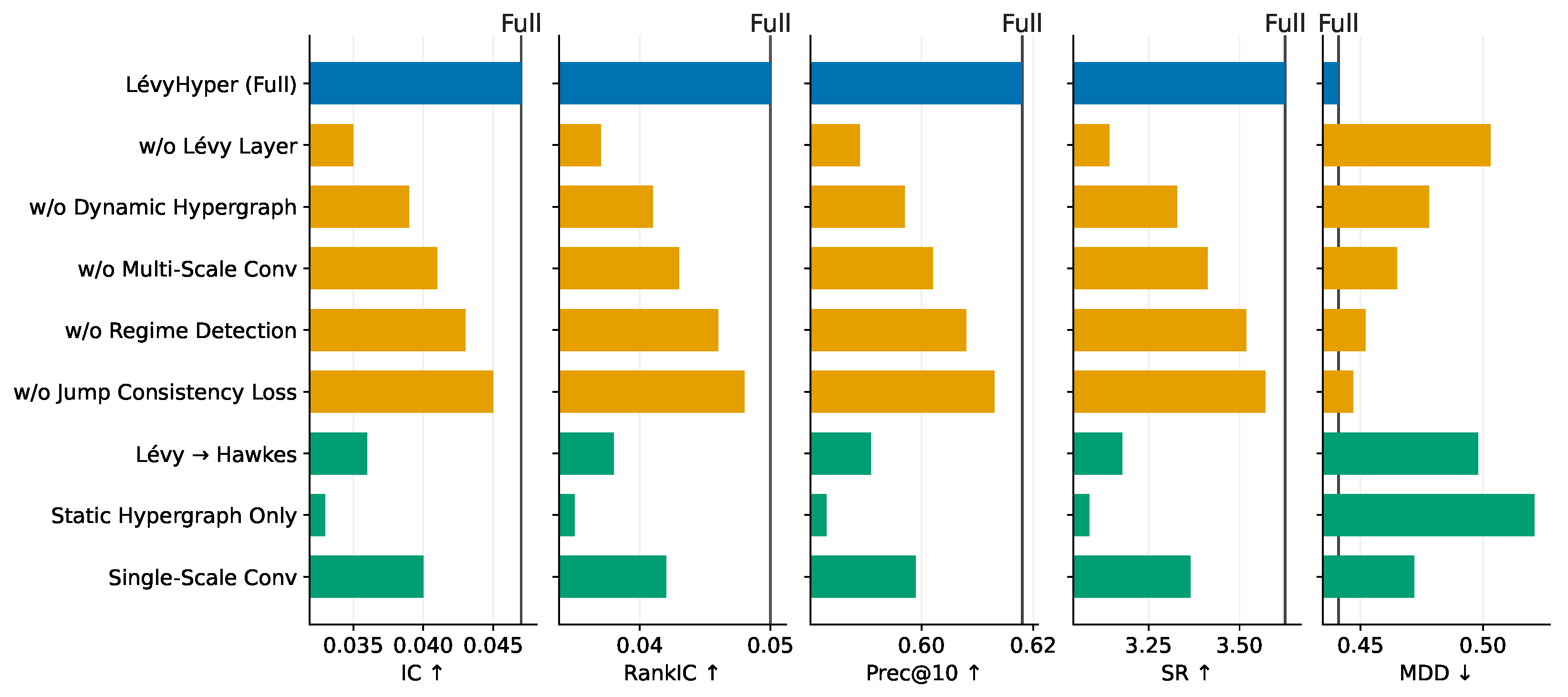
To systematically understand the contribution of each architectural component to LévyHyper’s overall performance, we conduct comprehensive ablation studies on the S&P 500 dataset by progressively removing or replacing individual modules while keeping all other components intact.

Table 5. Ablation study results on S&P 500 dataset. Each row removes or replaces one component from the full model while keeping all other components unchanged. All variants are trained with identical hyperparameters and evaluated on the same test splits.

Model Variant	IC	RankIC	Prec@10	SR	MDD
LévyHyper (Full)	0.047	0.050	0.618	3.625	0.441
Component Removal:
w/o Lévy Layer	0.035	0.037	0.589	3.142	0.503
w/o Dynamic Hypergraph	0.039	0.041	0.597	3.328	0.478
w/o Multi-Scale Conv	0.041	0.043	0.602	3.412	0.465
w/o Regime Detection	0.043	0.046	0.608	3.518	0.452
w/o Jump Consistency Loss	0.045	0.048	0.613	3.571	0.447
Component Replacement:
Lévy → Hawkes	0.036	0.038	0.591	3.178	0.498
Static Hypergraph Only	0.033	0.035	0.583	3.087	0.521
Single-Scale Conv	0.040	0.042	0.599	3.365	0.472

and Figure 3 present the results across both predictive metrics and portfolio performance measures, revealing the relative importance of each design choice. The ablation experiments are organized into two categories: complete removal of components to assess their necessity, and replacement with alternative implementations to validate our specific design decisions. Each variant is trained using identical hyperparameters and evaluated on the same test splits to ensure fair comparison, with performance degradation quantified relative to the full LévyHyper model.

The results demonstrate that the Lévy jump-diffusion layer constitutes the most critical component of our framework, as its removal causes the largest performance degradation across all metrics. Specifically, removing the Lévy layer leads to a 25.5% decrease in IC (from 0.047 to 0.035) and a 13.3% decrease in Sharpe ratio (from 3.625 to 3.142), while maximum drawdown increases substantially from 0.441 to 0.503, indicating significantly worse downside risk. This severe degradation confirms that explicitly modeling discontinuous jump dynamics is essential for capturing abrupt price movements that cannot be adequately represented through continuous diffusion processes alone. To validate our choice of Lévy processes over alternative point process models, we replace the Lévy layer with Hawkes processes, which have been previously applied to financial modeling for capturing self-exciting dynamics. The Hawkes variant achieves an IC of only 0.036, representing a 23.4% degradation compared to the full model, which demonstrates that Lévy processes’ ability to model heavy-tailed jump size distributions through flexible mixture models provides substantial advantages over Hawkes processes that primarily focus on temporal clustering of events. The dynamic hypergraph constructor also proves essential, as restricting the model to static industry-based hypergraphs alone causes a 29.8% decrease in IC (from 0.047 to 0.033) and a 14.8% decrease in Sharpe ratio (from 3.625 to 3.087). This substantial degradation validates our hypothesis that financial relationships evolve dynamically across market regimes, and that predefined static structures based solely on industry classifications cannot capture the complex, time-varying dependencies that emerge during different market conditions. The comparison between “w/o Dynamic Hypergraph” (which retains dynamic generation but removes the fusion mechanism) and “Static Hypergraph Only” (which uses only predefined structures) further reveals that both adaptive structure learning and the weighted fusion mechanism contribute meaningfully to performance.

The multi-scale spectral convolution module demonstrates significant value, as replacing it with single-scale convolution reduces IC by 14.9% (from 0.047 to 0.040) and Sharpe ratio by 7.2% (from 3.625 to 3.365), confirming that hierarchical temporal patterns at multiple resolutions—ranging from intraday fluctuations to monthly momentum—provide complementary information that enhances predictive accuracy. This finding aligns with financial theory suggesting that different market participants operate at different time scales, from high-frequency traders to long-term institutional investors, creating multi-resolution patterns in price dynamics. The regime detection mechanism, which adaptively weights the fusion between predefined and dynamic hypergraphs based on detected market states, contributes an 8.5% improvement in IC (comparing 0.047 to 0.043), demonstrating that explicit modeling of regime transitions enables the model to adjust its relational structure appropriately during shifts between normal and crisis periods. Finally, the jump consistency loss, which encourages the Lévy layer to produce interpretable jump predictions that align with empirically observed extreme returns, provides a 4.3% IC improvement (comparing 0.047 to 0.045). While this auxiliary loss yields the smallest individual contribution among all components, it serves an important role in regularizing the jump-diffusion module to learn physically meaningful parameters rather than overfitting to training data noise. Collectively, these ablation results validate that each component of LévyHyper addresses a specific limitation of existing methods, and that their synergistic integration—combining discontinuous jump modeling, adaptive relational learning, multi-scale temporal analysis, and regime-aware fusion—is necessary to achieve state-of-the-art performance in financial forecasting.

4.7. Computational Cost

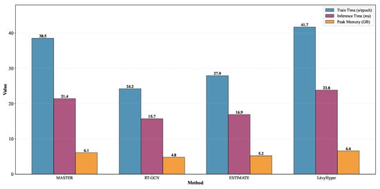
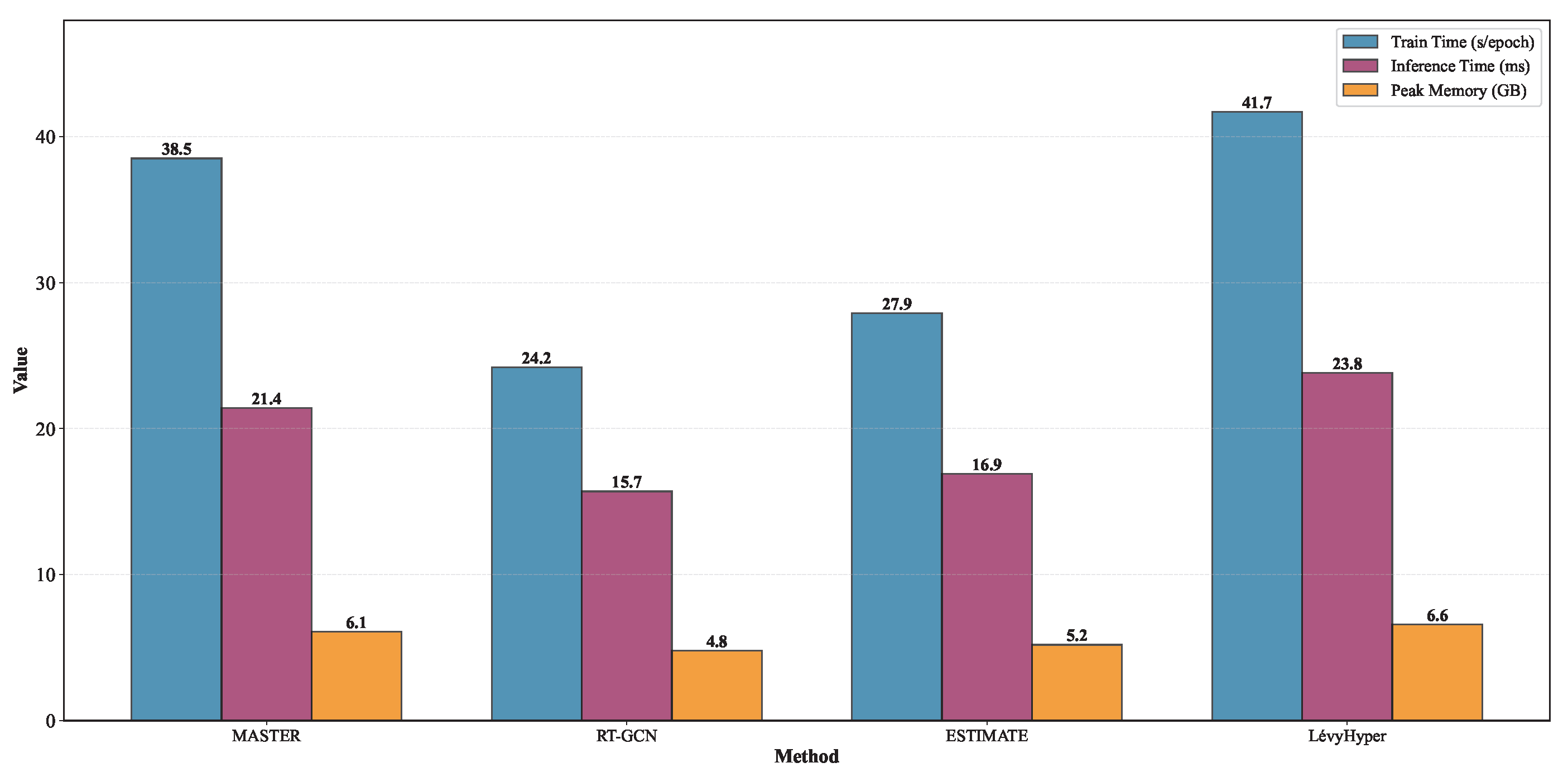
As discussed in Section 3.5.4, our computational complexity analysis assumes bounded hyperedge size and bounded number of hyperedges, which are explicitly enforced in our implementation with $\left|E\right|=95$ total hyperedges and mean hyperedge size ${\overline{d}}_e\approx 25$. To quantify the computational overhead introduced by jump-aware temporal modeling and dynamic hypergraph reasoning, we report training and inference cost on an NVIDIA A100 GPU. We measure training time per epoch, inference time per test day over the full universe (463 stocks), and peak GPU memory. The result is shown in Figure 4. LévyHyper incurs moderate overhead relative to graph/hypergraph baselines due to the jump-aware temporal module and dynamic hypergraph construction.

5. Conclusions

This paper propose LévyHyper, a novel framework for stock price forecasting that addresses three key challenges: modeling discontinuous price dynamics, capturing time-varying higher-order market relationships, and integrating multi-scale temporal dynamics with relational structures. LévyHyper introduces three key innovations. First, a Lévy jump-diffusion layer with neural-parameterized intensities explicitly models price jumps. Second, a regime-adaptive dynamic hypergraph constructor captures time-varying higher-order relationships. Third, a multi-scale spectral hypergraph convolution module integrates multi-resolution temporal and relational patterns. Experiments on S&P 500 data demonstrate its effectiveness, achieving 104% improvement in IC, 78% in RankIC, and 16.2% in Sharpe ratio compared to the strongest baseline. Ablation studies confirm the contribution of each component, and portfolio backtesting shows robust risk-adjusted performance with lower maximum drawdown.

Future work includes extending to multivariate Lévy processes, incorporating alternative data sources such as news and macro indicators, and developing online learning variants for high-frequency trading. LévyHyper advances the integration of stochastic processes and deep learning, offering promising directions for financial forecasting research.

Limitations and Future Work

Our experimental evaluation is conducted exclusively on S&P 500 data spanning 2010–2019, which represents a single market environment with relatively homogeneous characteristics. While the 10-phase evaluation protocol provides robustness across different time periods and market conditions within this setting, we cannot claim that the observed improvements generalize to fundamentally different market structures, asset classes, or geographical regions without additional empirical validation. Future work should extend LévyHyper’s evaluation to additional datasets including emerging markets (e.g., Chinese A-shares, Indian equities), non-equity assets (e.g., commodities, cryptocurrencies), and conduct cross-market transfer learning experiments where models trained on S&P 500 are tested on other markets to assess the portability of learned representations and the robustness of the three core innovations across diverse market structures. Additionally, extending to multivariate Lévy processes, incorporating alternative data sources such as news and macro indicators, and developing online learning variants for high-frequency trading represent promising directions for advancing the integration of stochastic processes and deep learning in financial forecasting.

References

- Engle, R.F. Autoregressive conditional heteroscedasticity with estimates of the variance of United Kingdom inflation. Econometrica 1982, 50, 987–1007. [Google Scholar] [CrossRef] [Scilit]
- Bollerslev, T. Generalized autoregressive conditional heteroskedasticity. J. Econom. 1986, 31, 307–327. [Google Scholar] [CrossRef] [Scilit]
- Andersen, T.G.; Bollerslev, T.; Diebold, F.X. Roughing it up: Including jump components in the measurement, modeling, and forecasting of return volatility. Rev. Econ. Stat. 2007, 89, 701–720. [Google Scholar] [CrossRef] [Scilit]
- Corsi, F. A simple approximate long-memory model of realized volatility. J. Financ. Econom. 2009, 7, 174–196. [Google Scholar] [CrossRef] [Scilit]
- Chen, W.; Yeo, C.K.; Lau, C.T.; Lee, B.S. A novel graph convolutional feature based convolutional neural network for stock trend prediction. Inf. Sci. 2021, 556, 67–94. [Google Scholar] [CrossRef] [Scilit]
- Feng, F.; He, X.; Wang, X.; Luo, C.; Liu, Y.; Chua, T.S. Temporal relational ranking for stock prediction. In Proceedings of the ACM Transactions on Information Systems; ACM: New York, NY, USA, 2019; Volume 37, pp. 1–30. [Google Scholar]
- Tao, Y.; Li, L. CQEformer: A Causal and Query-Enhanced Transformer Variant for Time-Series Forecasting. Mathematics 2025, 13, 3750. [Google Scholar] [CrossRef] [Scilit]
- Ding, Q.; Wu, S.; Sun, H.; Guo, J.; Guo, J. Hierarchical multi-scale Gaussian transformer for stock movement prediction. In Proceedings of the Twenty-Ninth International Joint Conference on Artificial Intelligence; ACM: New York, NY, USA, 2021; pp. 4640–4646. [Google Scholar]
- Ren, A.; Duan, Y.; Liu, J. Multiscale Bootstrap Correction for Random Forest Voting: A Statistical Inference Approach to Stock Index Trend Prediction. Mathematics 2025, 13, 3601. [Google Scholar] [CrossRef] [Scilit]
- Lee, M.C. A Hybrid EGARCH–Informer Model with Consistent Risk Calibration for Volatility and CVaR Forecasting. Mathematics 2025, 13, 3108. [Google Scholar] [CrossRef] [Scilit]
- Sawhney, R.; Agarwal, S.; Wadhwa, A.; Derr, T.; Shah, R.R. Stock selection via spatiotemporal hypergraph attention network: A learning to rank approach. In Proceedings of the AAAI Conference on Artificial Intelligence; AAAI Press: Washington, DC, USA, 2021; Volume 35, pp. 497–504. [Google Scholar]
- Lazcano, A.; Herrera, P.J.; Monge, M. A Combined Model Based on Recurrent Neural Networks and Graph Convolutional Networks for Financial Time Series Forecasting. Mathematics 2023, 11, 224. [Google Scholar] [CrossRef] [Scilit]
- Huang, X.; Tauchen, G. The relative contribution of jumps to total price variance. J. Financ. Econom. 2005, 3, 456–499. [Google Scholar]
- Hawkes, A.G. Spectra of some self-exciting and mutually exciting point processes. Biometrika 1971, 58, 83–90. [Google Scholar] [CrossRef]
- Huynh, T.T.; Nguyen, M.H.; Nguyen, T.T.; Nguyen, P.L.; Weidlich, M.; Yin, H.; Nguyen, Q.V.H. Efficient integration of multi-order dynamics and internal dynamics in stock movement prediction. In Proceedings of the Sixteenth ACM International Conference on Web Search and Data Mining; ACM: New York, NY, USA, 2023; pp. 850–858. [Google Scholar]
- Balcilar, M.; Ozdemir, Z.A.; Ozdemir, H.; Wohar, M.E. Crude oil futures contracts and commodity markets: New evidence from a TVP-VAR extended joint connectedness approach. Resour. Policy 2021, 73, 102219. [Google Scholar] [CrossRef] [Scilit]
- Zheng, S.; Zhu, J.; Ma, K.; Wang, T. Temporal and heterogeneous graph neural network for financial time series prediction. Inf. Sci. 2023, 623, 783–797. [Google Scholar]
- Li, T.; Cheng, Z.; Zhang, Y.; Chen, L. MASTER: Market-guided stock transformer for stock price forecasting. Pattern Recognit. 2024, 145, 109947. [Google Scholar] [CrossRef] [Scilit]
- Jin, S.; Wang, X.; Meng, Q. Spatial memory-augmented visual navigation based on hierarchical deep reinforcement learning in unknown environments. Knowl.-Based Syst. 2024, 285, 111358. [Google Scholar] [CrossRef] [Scilit]
- Qian, H.; Jin, S.; Chen, L. I2KEN: Intra-Domain and Inter-Domain Knowledge Enhancement Network for Lifelong Loop Closure Detection. IEEE Robot. Autom. Lett. 2025, 10, 8722–8729. [Google Scholar] [CrossRef] [Scilit]
- Hochreiter, S.; Schmidhuber, J. Long short-term memory. Neural Comput. 1997, 9, 1735–1780. [Google Scholar] [CrossRef] [Scilit]
- Vaswani, A.; Shazeer, N.; Parmar, N.; Uszkoreit, J.; Jones, L.; Gomez, A.N.; Kaiser, Ł.; Polosukhin, I. Attention is all you need. Adv. Neural Inf. Process. Syst. 2017, 30, 5998–6008. [Google Scholar]
- Scarselli, F.; Gori, M.; Tsoi, A.C.; Hagenbuchner, M.; Monfardini, G. The graph neural network model. IEEE Trans. Neural Netw. 2008, 20, 61–80. [Google Scholar] [CrossRef] [Scilit] [PubMed]
- Matsunaga, D.; Suzumura, T.; Takahashi, T. Exploring graph neural networks for stock market predictions with rolling window analysis. In Proceedings of the NeurIPS Workshop on Machine Learning for Autonomous Driving, Vancouver, BC, Canada, 13–14 December 2019. [Google Scholar]
- Zhang, D.; Hu, M.; Ji, Q. Financial markets under the global pandemic of COVID-19. Financ. Res. Lett. 2020, 36, 101528. [Google Scholar] [CrossRef] [Scilit] [PubMed]
- Cont, R.; Tankov, P. Financial Modelling with Jump Processes; Chapman and Hall/CRC: Boca Raton, FL, USA, 2004. [Google Scholar]
- Jang, E.; Gu, S.; Poole, B. Categorical reparameterization with gumbel-softmax. In Proceedings of the International Conference on Learning Representations, Toulon, France, 24–26 April 2017. [Google Scholar]
- Kipf, T.N.; Welling, M. Semi-supervised classification with graph convolutional networks. In Proceedings of the International Conference on Learning Representations, Toulon, France, 24–26 April 2017. [Google Scholar]
- Hammond, D.K.; Vandergheynst, P.; Gribonval, R. Wavelets on graphs via spectral graph theory. Appl. Comput. Harmon. Anal. 2011, 30, 129–150. [Google Scholar] [CrossRef] [Scilit]
- Kingma, D.P.; Ba, J. Adam: A Method for Stochastic Optimization; International Conference on Learning Representations: Appleton, WI, USA, 2015. [Google Scholar]
- Barndorff-Nielsen, O.E.; Shephard, N. Econometric analysis of realized covariation: High frequency based covariance, regression, and correlation in financial economics. Econometrica 2004, 72, 885–925. [Google Scholar] [CrossRef] [Scilit]
- Barndorff-Nielsen, O.E.; Kinnebrock, S.; Shephard, N. Measuring Downside Risk-Realised Semivariance. CREATES Research Paper. 2008. Available online: https://econpapers.repec.org/paper/aahcreate/2008-42.htm (accessed on 12 November 2025).
Disclaimer/Publisher’s Note: The statements, opinions and data contained in all publications are solely those of the individual author(s) and contributor(s) and not of MDPI and/or the editor(s). MDPI and/or the editor(s) disclaim responsibility for any injury to people or property resulting from any ideas, methods, instructions or products referred to in the content. |
© 2026 by the authors. Licensee MDPI, Basel, Switzerland. This article is an open access article distributed under the terms and conditions of the Creative Commons Attribution (CC BY) license.