Augmentation of Small Ultrasound Databases: A Practical Approach

Abstract

Generative Adversarial Networks (GANs) have emerged as a promising tool for augmenting medical image datasets used by AI solutions. However, GANs trained on small datasets (300–500 images) frequently encounter mode collapse, overfitting, and instability, which hinder their practical application. Many GAN-generated images look unrealistic. The Enhanced Deep Convolutional GAN (EDCGAN) is introduced to generate high-quality synthetic images of breast US (BUS). The model includes an experimental design for the Discriminator and Generator. The main components are spectral normalization (SN), the Squeeze-and-Excitation (SE) block, and the Scaled Exponential Linear Unit (SELU). One of the basic versions of DCGAN is considered for the proposed modifications. The stopping criteria are based on the convergence of the smoothed loss function and the constraints imposed on the Discriminator. The contribution is a combination of the above modifications and postprocessing based on the visual evaluation by radiologists and selected image processing metrics. The Inception Score (IS), the Structural Similarity Index (SSIM), and the Mean Squared Error (MSE) comply with the results obtained in the preceding works. The efficiency of augmenting the US data has been verified on a DL classification based on ResNet-18. The tests against training on a non-augmented data outperform ResNet by 5% and by the data augmented by the previous DCGAN by 3%. These numbers are substantial since this variant of ResNet has been pre-trained on 1000 categories by ImageNet-1K, including 1.28 million images. Additionally, the model wins the “Guess-the-real-image” game, competing with seven preceding GANs.

1. Introduction

Breast cancer accounts for about 25% of all cancers worldwide, being the leading cause of cancer-related deaths among women [1]. Early and accurate detection is critical for improving survival rates, facilitating timely intervention, and ensuring personalized treatment. Conventional imaging modalities, such as mammography and ultrasound (US), play a central role in breast cancer screening. However, they are still hindered by numerous limitations. Mammography, for instance, demonstrates reduced sensitivity in screening individuals with dense breast tissue, leading to a higher incidence of false negatives. Radiologists are usually able to detect tumors in those US images. This paper addresses these challenges by proposing an EDCGAN designed to generate synthetic breast ultrasound images (BUS) under data-scarce conditions. Our approach integrates several modifications. Several metrics are used to evaluate the quality of synthetic images, alongside evaluations by experienced radiologists. The stopping criterion includes the convergence of the smoothed loss function and the realistic constraints imposed on the Generator. The efficiency of augmenting the US data has been verified on a DL classification based on ResNet-18 [2]. The tests against training on non-augmented data outperform ResNet by 5% and by the data augmented by the previous DCGAN by 3%. These numbers are substantial since this variant of ResNet has been pre-trained on 1000 categories by ImageNet-1K, including 1.28 million images. Additionally, the model wins the “Guess-the-real-image” game, competing with seven preceding GANs to deceive experienced radiologists. An interested reader may download and replicate the proposed GAN at github.com by https://rb.gy/tbb43k (accessed on 31 January 2025).

2. Related Work

2.1. Data Scarcity in Medical Image Processing

The recent review (Upadhyay and Bhandari, 2024) [3] indicates that data scarcity is one of the biggest challenges for learning-based segmentation, classification, and denoising models, which represent a standard triad of medical image processing. Early segmentation and classification models rely on techniques that have a solid theoretical background, such as a variety of clustering methods: fuzzy C-means, support vector machines, decision trees, etc. Segmentation models apply template matching, active contours, and level set methods. The latter two have a solid foundation in the calculus of variations and partial differential equations. Tuning these models does not require large amounts of data but rather domain knowledge, research experience, and intuition. In contrast, DL models require large datasets having sufficient variety. There are several well-established criteria to detect when optimal performance has been achieved [4]. The optimized DL model is usually not affected by image quality issues, such as moderate noise, low contrast, and broken boundaries (a significant issue for deformable models). Ten years ago, LeCun et al published a paper in “Nature” [5] in which they noted that the availability of datasets used to train AI was limited due to the specialized expertise required. To overcome these limitations, conventional data augmentation techniques—such as rotations, flips, cropping, scaling, and color variations—have become widely adopted methods for expanding training datasets. However, they are usually not sufficient for quality training, although the traditional augmentation methods for BUS image processing have been thoroughly analyzed and experimented with [6]. GANs [7] have gained significant attention as powerful tools for augmenting medical image datasets by generating synthetic images that closely resemble real scans [8,9,10]. However, modern medical image processing faces increased challenges due to the development of new imaging technologies and the massive integration of AI with segmentation and classification models [11,12,13,14,15,16]. Denoising medical image models have also been successfully augmented (see, for instance, [17,18,19,20,21]). From the viewpoint of data quality and availability, the DL methods include supervised learning (such as earlier CNNs), unsupervised learning (such as GANs), and a combination of supervised and unsupervised learning techniques [22]. With the advancement of digital technology, large amounts of labeled image data are now available in different application domains. As far as medical imaging is concerned, large labeled datasets remain a challenge due to data privacy issues, costs, the expertise required for the annotation process [23], and even issues related to “data discrimination” [24] and “medical data terrorism,” when the AI system has been injected with "toxic" samples, leading to incorrect conclusions or unrealistic images [25]. Therefore, GANs data augmentation is part of the evolving combination of supervised, semi-supervised, and self-learning approaches, where GANs themselves are considered self-supervised or semi-supervised DL neural networks. Manual labeling requires a significant amount of time, and errors are possible. Zhang et al (2025) [26] remark that subjective human labeling may result in ambiguous semantic models. However, conventional self-supervised learning still requires the establishment of strongly differential positive and negative pairs. In turn, this often relies on in-depth domain knowledge and medical expertise. A self-augmentation approach has been proposed in [26] based on batch fusion. We conjecture that a modification of the proposed model might be applied to the adaptive batch augmentation proposed by Zhang [26]. However, a straightforward practical application is the augmentation of startups being developed from scratch, the improvement of pre-trained models, or even the use of GAN images in education, for instance, in multiple-choice tests for medical schools. For an extended discussion of data scarcity and supervised vs. unsupervised learning, we refer the reader to excellent reviews in [3,26] and the most recent work [27].

2.2. GANs in Medical Image Processing

GANs apply to a variety of medical imaging tasks, including image-to-image translation, segmentation, classification, registration, and many others [28]. GANs have been used for translating between different imaging modalities, such as converting CT scans to synthetic MRI or US images [29]. They have shown much promise in image segmentation, such as the Automated Brain Tumor Segmentation [30]. One of the most important tasks is data augmentation. However, clinical adoption is often hindered by the lack of standardized data protocols. This affects the quality, consistency, and realism of the generated images. Several studies, such as [31], address critical challenges, including preserving anatomical details and mitigating training instability. Ref. [32] proves that augmenting data using GAN-generated images improves the F1-classification score from 62% to 74%. Ref. [33] demonstrates significant MSE, SSIM, and PSNR values for BUS using CCA and Nerve (carotid artery and nerve datasets). However, the application of GANs to BUS image synthesis remains relatively underexplored. We conjecture that one of the reasons is the variety of deterministic data augmentation methods applicable to BUS medical imagery [6]. Nevertheless, recent research works such as [34] (2024) show the excellent potential of GANs. The authors report promising results from a small database of calcified and cystic thyroid gland nodules. The generated images are evaluated using the Fréchet Inception Distance (FID) test and human observation. Nevertheless, the stopping criteria, stability, convergence, and quality of the synthetic images remain open problems.

2.3. Enhancements of DCGANs

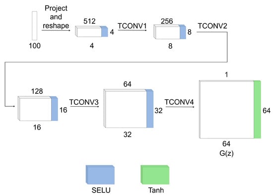
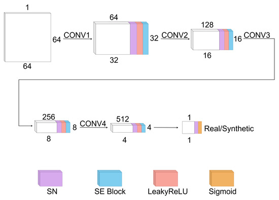
DCGANs [35] enable high-quality, realistic images while mitigating common issues such as mode collapse and training instability. As opposed to original GANs, which employ fully connected layers, DCGANs [35] are equipped with convolutional layers. According to [36], DCGANs are the most popular GANs to date. Since this is often the de facto basic GAN that one can implement, in this paper, we use a basic architecture shown in Figure 1 and Figure 2. Note that several works show the use of DCGAN to augment relatively small databases (see, for instance, [31]); however, it is not clear whether it is possible to substantially increase the database (for instance, twofold). The competing WGANs [37] treat the problem of instability by introducing the Wasserstein loss. Consequently, WGANs are characterized by a small stochastic gradient, whereas conventional GANs typically have a flat gradient in the middle and a steep gradient elsewhere. Consequently, WGANs are characterized by a small stochastic gradient, while conventional GANs typically exhibit a flat gradient in the middle and a steep gradient elsewhere. As a result, the variance of WGAN is usually smaller.

Figure 1. Generator network.

Figure 2. Discriminator network.

Further, note the gradient penalty method, which enforces the Lipschitz condition  [38]. The modification stabilizes training and helps mitigate issues such as mode collapse  [39] and vanishing gradients. Least Squares GANs (LSGANs) [40] replace the traditional binary cross-entropy loss with a least squares loss function. This addresses the vanishing gradient problem and encourages sharper, more realistic image generation. Spectral Normalization GANs (SNGANs) [41] apply to the weights of the Generator and Discriminator. This prevents instability and does not allow for the destabilization of the model. Information GANs (InfoGANs) [42] introduce a mutual information term in the loss function, encouraging the Generator to produce diverse outputs. This modification enables the Generator to learn meaningful features, resulting in interpretable and distinct outputs that can be controlled by manipulating the latent variables. In this paper, we integrate some of the above tweaks into the DCGAN framework and show that, with appropriate training and postprocessing, DCGAN is capable of producing acceptable augmentation results.

3. Contribution

This study introduces a modification of DGAN tailored to generate quality synthetic BUS images under data-scarce conditions. The model integrates spectral normalization (SN) [41], Squeeze-and-Excitation (SE-block) [43], and Scaled Exponential Linear Unit (SELU) activation [44], along with label smoothing [45] and asymmetric learning rates. The specific stopping criterion combines the convergence of the smoothed loss function with the experimental constraints imposed on the Discriminator. Postprocessing allows for the detection of unrealistic and repeated outputs using experimentally selected quality measures. The model relies on the visual analysis conducted by trained radiologists. However, it presents a straightforward and simple approach to successful augmentation. The proposed EDCGAN has been verified for augmenting a small database for DL classification based on ResNet-18. The tests against training on non-augmented data outperform the standard ResNet by 5% and by the data augmented by the previous DCGAN by 3%. These numbers are substantial since this variant of ResNet has been pre-trained on 1000 categories by ImageNet-1K, including 1.28 million images. Finally, an innovative “Guess-the-real-image” has been introduced, where the competing GANs are supposed to deceive the radiologists. The proposed model wins the game against seven competing GANs with a notable advantage.

4. Experimental Setup

The study utilizes a subset of the BUS dataset [46], consisting of 780 grayscale US images from 600 female patients aged 25 to 75 years. The dataset was collected in 2018 by Baheya Hospital of Egypt using the LOGIQ E9 and LOGIQ E9 Agile ultrasound systems. The data have been categorized into three classes: normal, benign, and malignant. 593 images without markings were selected. In order to reduce computational load and generate a large number (thousands) of synthetic images, the real images have been scaled to $64\times 64$. The basic DCGAN designed for this size of images has been selected as the backbone, as this type has recently become a de-facto baseline model for modification and adaptation to specific datasets and types of images [36]. The images have been normalized to the range $[0, 255]$. The focus is on the efficiency of the combination of the SE-block, SELU, SN, postprocessing, and evaluation. Apart from dealing with a limited dataset, the limitations of computational time are also taken into account. We confine ourselves to approximately 1 h of training time on a common computer with an i7 processor, an NVIDIA GeForce RTX 3050 graphics card, 4 GB of memory, and CUDA version 12.7. The training stops if the model converges (see Section 6) or if the prescribed computational time has elapsed. The resulting images are evaluated using selected metrics, both visually by computer science experts specializing in ultrasound image processing and by trained radiologists.

5. Model Structure

In order to test the proposed modifications, one of the most popular GAN structures is illustrated in Figure 1 and Figure 2.

5.1. Generator

The Generator in Figure 1 runs the random input vector through a sequence of transposed convolutions to progressively up-sample and refine it into synthesized images. The layers double the spatial resolution of the input and simultaneously reduce the number of feature maps. The up-sampling layers are followed by SELU activation [44]. The output of the Generator is processed by the Tanh activation, mapping it onto the desired range.

5.2. Discriminator

The Discriminator is a sequence of convolutional layers that progressively down-samples the input image while expanding the number of feature maps, enabling the network to capture fine details and complex patterns. Each convolutional layer is followed by a LeakyReLU activation [47]. The SN and SE blocks are applied to all layers. The output layer is subjected to a sigmoid activation function to produce an estimate in the range [0, 1].

6. Loss Functions

The learning rates selected by trial and error are $1\times {10}^{-4}$ and $3\times {10}^{-4}$ for the Generator and the Discriminator, respectively. This difference allows for faster adaptation while maintaining stable updates for the Generator. Label smoothing is applied to handle overfitting, preventing the Discriminator from becoming overly confident by assigning the real images a value of 0.9 and the synthetic images a value of 0.1. A batch size of 8 is used to balance computational efficiency and training stability while addressing the constraints imposed by GPU memory. The model is trained for a maximum of 2 h. The experiments show that it provides sufficient time for the network to achieve synthesis, subject to the proposed modifications.

6.1. Loss Function and Optimizer

Training follows the standard adversarial setup, where the Generator and Discriminator are trained simultaneously within the framework of a two-player minimax game. The Generator aims to produce realistic images that can fool the Discriminator, while the Discriminator classifies images as real or synthetic. Training of the Discriminator is performed using a batch of real images and a batch of generated images. The Discriminator maximizes the probability of correct classification as given by the standard loss function:

$${\mathcal{L}}_D=-{\mathbb{E}}_{x\sim p_{\mathrm{data}}\left(x\right)}[logD\left(x\right)]-{\mathbb{E}}_{z\sim p_z\left(z\right)}[log(1-D\left(G\left(z\right)\right))],$$

(1)

where $\mathbb{E}$ denotes the expectation operator, x represents a sample from the dataset, $D\left(x\right)$ denotes the Discriminator’s output, z is the input vector, and $G\left(z\right)$ generates the synthetic data, whereas $D\left(G\right(z\left)\right)$ denotes the Discriminator’s output. Based on the feedback from the Discriminator, the Generator tries to minimize the Discriminator’s ability to distinguish between real and generated images. The Generator is used as follows:

$${\mathcal{L}}_G=-{\mathbb{E}}_{z\sim p_z\left(z\right)}[logD\left(G\left(z\right)\right)].$$

(2)

The updates are performed by the Adam optimizer [48] provided by

$$\begin{array}{cc}\hfill m_t& ={\beta }_1{m}_{t-1}+(1-{\beta }_1){\nabla }_{\theta }{\mathcal{L}}_G^{\left(t\right)},\hfill \\ \hfill v_t& ={\beta }_2{v}_{t-1}+(1-{\beta }_2){\left({\nabla }_{\theta }{\mathcal{L}}_G^{\left(t\right)}\right)}^2,\hfill \\ \hfill {\widehat{m}}_t& ={\displaystyle \frac{m_t}{1-{\beta }_1^t}},{\widehat{v}}_t={\displaystyle \frac{v_t}{1-{\beta }_2^t}},\hfill \\ \hfill {\theta }_t& ={\theta }_{t-1}-\alpha {\displaystyle \frac{{\widehat{m}}_t}{\sqrt{{\widehat{v}}_t}+ϵ}},\hfill \end{array}$$

(3)

where ${\nabla }_{\theta }$ is the stochastic gradient, and $m_t$ and $v_t$ are the first- and second-moment estimates of the gradients of the loss function, respectively, while ${\widehat{m}}_t$ and ${\widehat{v}}_t$ are their bias-corrected counterparts. The step size is governed by the learning rate $\alpha$, and $ϵ$ prevents division by zero. ${\beta }_1$ = 0.5 and ${\beta }_2$ = 0.999 have been determined experimentally.

6.2. Stopping Criteria

The objective functions of GANs lack theoretical convergence to a unique solution in which the two probability distributions of the real and fake images are identical. Our analysis is based on practical experiments and the typical behavior of ${\mathcal{L}}_G$ and ${\mathcal{L}}_D$. Usually, GANs do not converge in the sense of classical numerical analysis. Moreover, they may converge to nonsensical values, such as 0 or 1. In this case, the gradients are close to zero at both ends, and the Discriminator does not provide realistic feedback (the vanishing gradient problem). The converged network may also output repetitive images, which are not useful for efficient augmentation (mode collapse). The loss function usually oscillates. Consequently, we suggest smoothing the loss and detecting convergence using the moving average, i.e.,

$$|L_a^{n+1}-L_a^n|<{\mathrm{\Delta }}_a,$$

(4)

where n is the epoch number and $L_a^n$ is the moving average of L on the interval $[n-k,n+k]$, and k, ${\mathrm{\Delta }}_a$ are the experimental thresholds. In order to exclude random peaks of L, the moving average $L_a$ is calculated without outliers, using the interquartile range (IQR). Furthermore, the acceptance rate $D_{\mathrm{acc}}$ of the Discriminator must not be below 5%. Otherwise, the model is considered divergent. The interval for detecting acceptable images is determined by supervised classification. It is a data-dependent step that requires a manual evaluation of the images. However, we claim that this is a practical method when the database consists of a small number of training samples. In summary, for the loss function $L_a$, the Algorithm 1 works as follows:

Algorithm 1: Summary of the loss function $L_a$

1. Input: Array $L_a$ and the size of the interval for moving avarage k 2. For $[n-k_1,n+k_1]$, calculate IQR. 3. $L_{a,i}\in \mathrm{IQR} L_{\mathrm{IQR},i}\to L_{a,i}$ 4. $L_{\mathrm{smooth},i}->\mathrm{MovingAverage}\left(L_{\mathrm{IQR},i}\right)$ 5. If $\left|\right|L_{\mathrm{smooth}}^{n+1}-L_{\mathrm{smooth}}^n\left|\right|\le {\mathrm{\Delta }}_a$ & $D_{acc}\le 5\%\to \mathrm{success}$. 6. If $\mathrm{calc}\text{-}\mathrm{time}>2h\to \mathrm{fail},\mathrm{initialize}\mathrm{a}\mathrm{new}\mathrm{random}\mathrm{image}.$

The IQR and MovingAverage are usually available in the libraries of modern programming languages, for instance, scipy.stats and Panda of Python (https://www.python.org/) or the #include <vector>, #include <numeric>class to use SimpleMovingAverage - C++.

7. Image Metrics

This section offers a short overview of the most important image similarity scores. The Inception Score (a trained statistical score applicable to an image set), the Structural Similarity Index (a non-reference score), and the Mean Squared Error (a reference score) are used for the proposed postprocessing step.

7.1. Inception Score (IS)

The Inception Score (IS) [49] is a recognized metric for evaluating the quality and diversity of images produced by GAN. The metric is shown to comply with human perception of the realism of synthetic images. The IS uses an Inception v3 Network pre-trained on ImageNet [50]. The IS implies a diversity of output images. One of the desired properties of the IS is that it does not require ground truth images. Therefore, it is ideal for situations involving a small dataset.

7.2. Structural Similarity Index (SSIM)

SSIM [51] includes luminance, contrast, and texture. This measure, aligned with human visual perception, ranges from 0 to 1, with a higher SSIM indicating that the synthetic image closely resembles the structural qualities of the reference image. When luminance, contrast, and texture are given equal weights,

$$\mathrm{SSIM}={\displaystyle \frac{(2{\mu }_x{\mu }_y+C_1)(2{\sigma }_{xy}+C_2)}{({\mu }_x^2+{\mu }_y^2+C_1)({\sigma }_x^2+{\sigma }_y^2+C_2)}},$$

(5)

where $x,y$ is the gray level of the images I and T to be compared, $\mu$ is the mean intensity, $\sigma$ is the standard deviation, and $C_1$ and $C_2$ are small constants. A statistical version of the above is MSSIM, which is the mean of all local SSIM values.

7.3. Edge Preservation Index (EPI)

The EPI is given by

$$\mathrm{EPI}(I,T)={\displaystyle \frac{{\sum }_{i}D{\left(I\right)}_{i}D{\left(T\right)}_i}{\sqrt{{\sum }_{i}D{\left(I\right)}_i^2{\sum }_{i}D{\left(T\right)}_i^2}}},$$

(6)

where $D\left(S\right)=\nabla S-E[\nabla S]$, T, and I are images to be compared.

7.4. Features Similarity Index Matrix (FSIM)

FSIM combines the image features in the frequency domain, extracted by the Fourier transform, with the gradients. Let $P_C$ and $G_M$ be the phase congruency map [52] and the map of the gradient magnitude. Then,

$$\mathrm{FSIM}(I,T)={\displaystyle \frac{{\sum }_i{S}_{P_C}{\left(I\right)}_i{S}_{P_C}{\left(T\right)}_i{S}_{P_m}(I,T)}{{\sum }_i{S}_{P_m}{(I,T)}_i}},$$

(7)

where

$$S_{P_C}={\displaystyle \frac{2S_{P_C}\left(I\right)S_{P_C}\left(T\right)+T_1}{S_{P_C}^2\left(I\right)+S_{P_C}^2\left(T\right)}},$$

(8)

$$S_{G_M}={\displaystyle \frac{2S_{G_M}\left(I\right)S_{G_M}\left(T\right)+T_2}{S_{G_M}^2\left(I\right)+S_{G_M}^2\left(T\right)}},$$

(9)

where $P_{C_m}=max(P_C\left(I\right),P_C\left(T\right))$, $T_1$, and $T_2$ are constants to avoid division by zero.

7.5. Mean Squared Error (MSE)

MSE is the squared average Euclidean distance between images I and T, given by

$$\mathrm{MSE}(I,T)={\displaystyle \frac{1}{N}}\sum _{i=1}^N{(x_i-y_i)}^2.$$

(10)

Although the MSE is essentially a non-statistical measure, its straightforward value could be particularly important for evaluating the structural fidelity of the generated images [53]. Nevertheless, MSE cannot be used blindly and must be tailored to a particular application. The average MMSE is defined as the mean of all pairs of MSE between two sets of images. Further, in the framework of this application, we define

$${\mathrm{MSE}}_{min}=\underset{I,T}{min}\mathrm{MSE}(I,T),$$

(11)

where I is a generated image or a set of images, and T is a set of training images (a batch or the entire training set). Further, the MSE-based PSNR is evaluated by

$$\mathrm{PSNR}(I,T)=10{log}_{10}{\displaystyle \frac{{(maxT)}^2}{\mathrm{MSE}}},$$

(12)

where T is the reference image. Although PSNR can be used to evaluate the difference between I and T, this measure is usually applied to image denoising. In the framework of GANs, some degree of diversity is required. Hence, the interpretation of PSNR is somewhat cumbersome. In this paper, MMSE and ${\mathrm{MSE}}_{min}$ are used.

7.6. Freshet Inception Distance

The FID requires a pre-trained Inception v3 model [50]. The deepest pooling layer (2048 elements) of Inception is then used to predict the features of the collection of real and generated images. The FID score is then calculated by

$$\mathrm{FID}=\left|\right|{\mu }_1-{\mu }_2{\left|\right|}^2+\mathrm{Tr}(S_1+S_2)-2\sqrt{S_1{S}_2},$$

where ${\mu }_1$ and ${\mu }_2$ denote the feature-wise means of the real and generated images (2048 elements), where each element is the mean across the images, whereas $S_1$ and $S_2$ are the covariance matrices for the real and generated feature vectors.

7.7. Visual Quality

While quantitative metrics provide valuable insights, they may not fully capture the perceptual quality and clinical relevance of the generated images. To address this limitation, a qualitative evaluation was performed. The visual analysis was conducted by expert radiologists tasked with distinguishing between real and generated images.

8. Testing the Model Enhancements

SELU activation function integrated into the Generator maintains the mean and variance of the processed data. This allows for stabilizing the gradients during backpropagation. SELU eliminates the need for batch normalization [54], contributing to better convergence compared to ReLU-type or Softmax types [55]. Table 1 shows a preliminary test of SELU vs. the standard activation function applied in the framework of this project.

The activation functions of the Discriminator follow the standard DCGANs scheme, characterized by the LeakyReLU activation, which is often considered a necessity for these types of GANs [47].

The Discriminator has also been modified as follows. SN [38] is applied to all convolutional layers to stabilize the training process by controlling the Lipschitz constant [56]. SN is a weight-based technique designed to stabilize training by constraining the Lipschitz constant, allowing for a better balance between the Generator and Discriminator. As a matter of fact, the initial prediction accuracy of the Discriminator, which is over 0.9, often does not allow for a properly stable state. As a result, the network in the simulation stage produces repeated images (diversity issue) or images that are too close to the training set. “Weakening” the Discriminator allows for the learning of generalizable features across the training distribution rather than memorizing features that are specific to the training data. In addition, the reduction in the Discriminator’s confidence helps mitigate the imbalance between the Generator and the Discriminator, allowing the Generator to receive consistent and informative feedback. Table 1 displays the preliminary tests of variation and the loss function during the first 100 epochs.

Table 1. Training stability across different activation functions.

Activation Function	Variance		Standard Deviation
	Generator	Discriminator	Generator	Discriminator
ReLU [55]	450.8382	0.2029	21.2330	0.4505
PReLU [57]	840.0590	1.4209	28.9838	1.1920
RReLU [58]	47.9511	0.3254	6.9247	0.5704
GELU [59]	1018.2862	1.2850	31.9106	1.1336
ELU [60]	38.8995	0.1148	6.2369	0.3389
Softmax [61]	306.0304	0.3354	17.4937	0.5791
SELU [44]	27.6596	0.1122	5.2592	0.3350

Table 1. Training stability across different activation functions.

Activation Function	Variance		Standard Deviation
	Generator	Discriminator	Generator	Discriminator
ReLU [55]	450.8382	0.2029	21.2330	0.4505
PReLU [57]	840.0590	1.4209	28.9838	1.1920
RReLU [58]	47.9511	0.3254	6.9247	0.5704
GELU [59]	1018.2862	1.2850	31.9106	1.1336
ELU [60]	38.8995	0.1148	6.2369	0.3389
Softmax [61]	306.0304	0.3354	17.4937	0.5791
SELU [44]	27.6596	0.1122	5.2592	0.3350

The Squeeze-and-Excitation (SE) block re-calibrates the feature maps by adaptively learning the importance of each feature layer. This enables the network to focus on the most relevant regions and features of the image. In other words, the importance of each layer is different. Hence, the features can be enhanced by extending the useful layers and reducing the useless layers [43]. The SN is based on the idea that the Discriminator must also stabilize the training process by controlling the Lipschitz constant [56]. Table 2 shows the contributions of each enhancement and their combinations. It is interesting that the SN has a significant impact on convergence, although it is a function of the Discriminator. SE alone does not notably change the loss function. However, it works well in combination with other enhancements.

Table 2. Convergence of EDCGAN with combinations of SN, SE, and SELU.

Combinations	Converged Models %
DCGAN/standard	70%
DCGAN/SELU	72%
DCGAN/SE	70%
DCGAN/SN	77%
DCGAN/SELU/SE	72%
DCGAN/SELU/SN	78%
DCGAN/SE/SN	78%
EDCGAN	81%

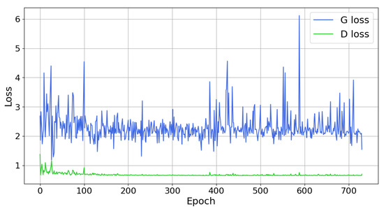
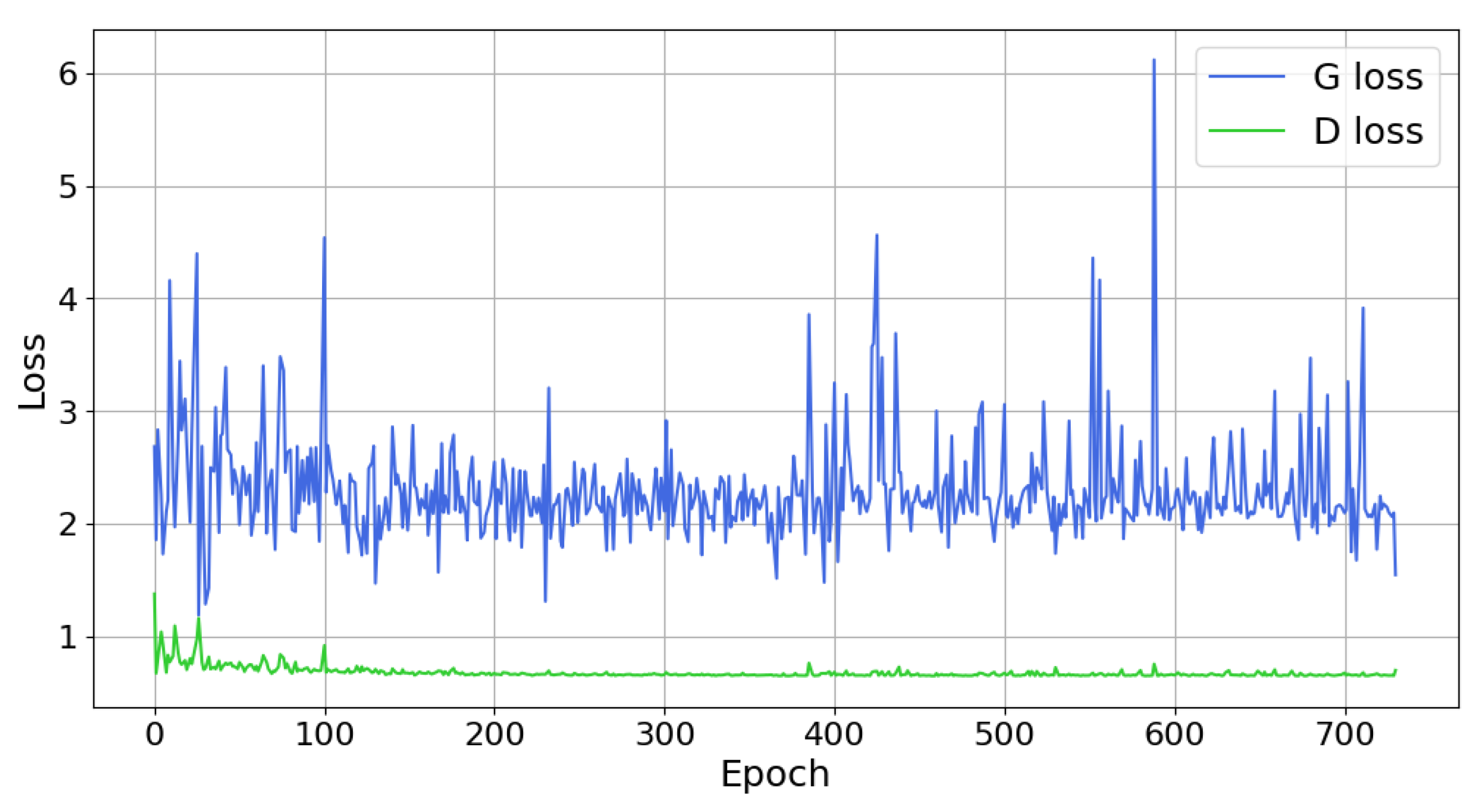
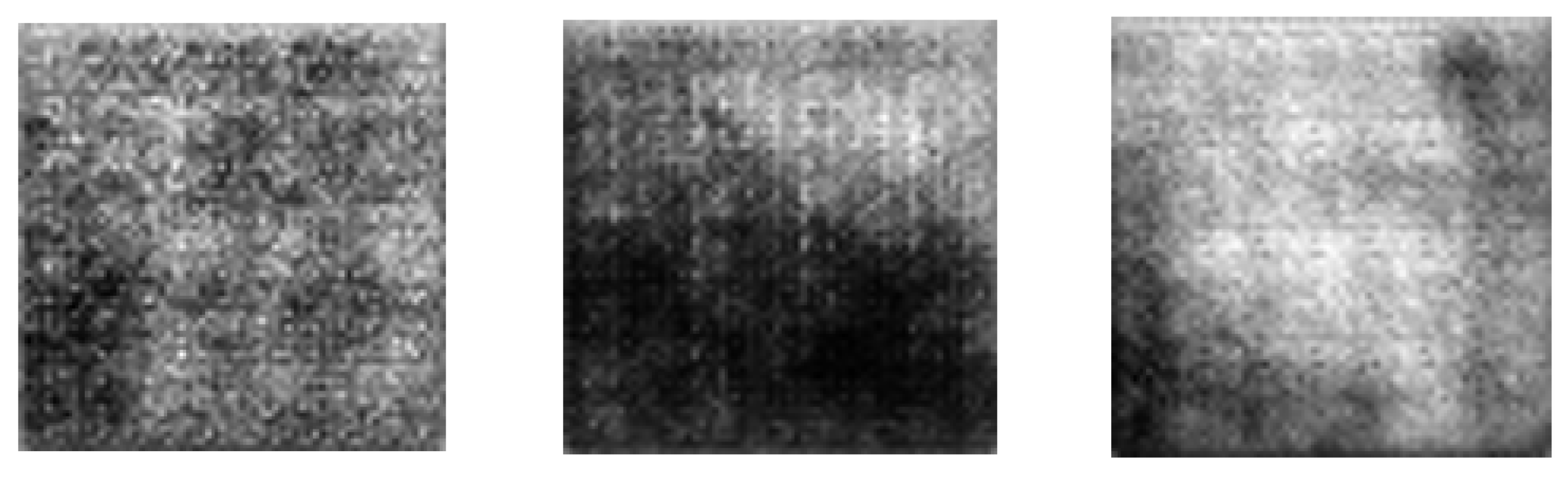
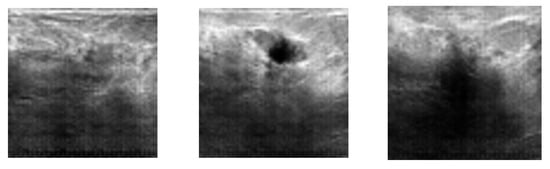
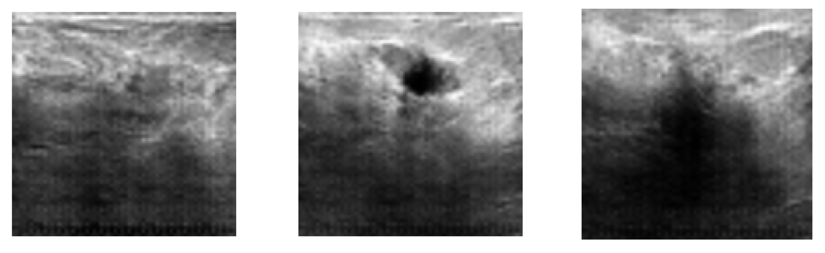
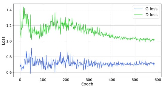
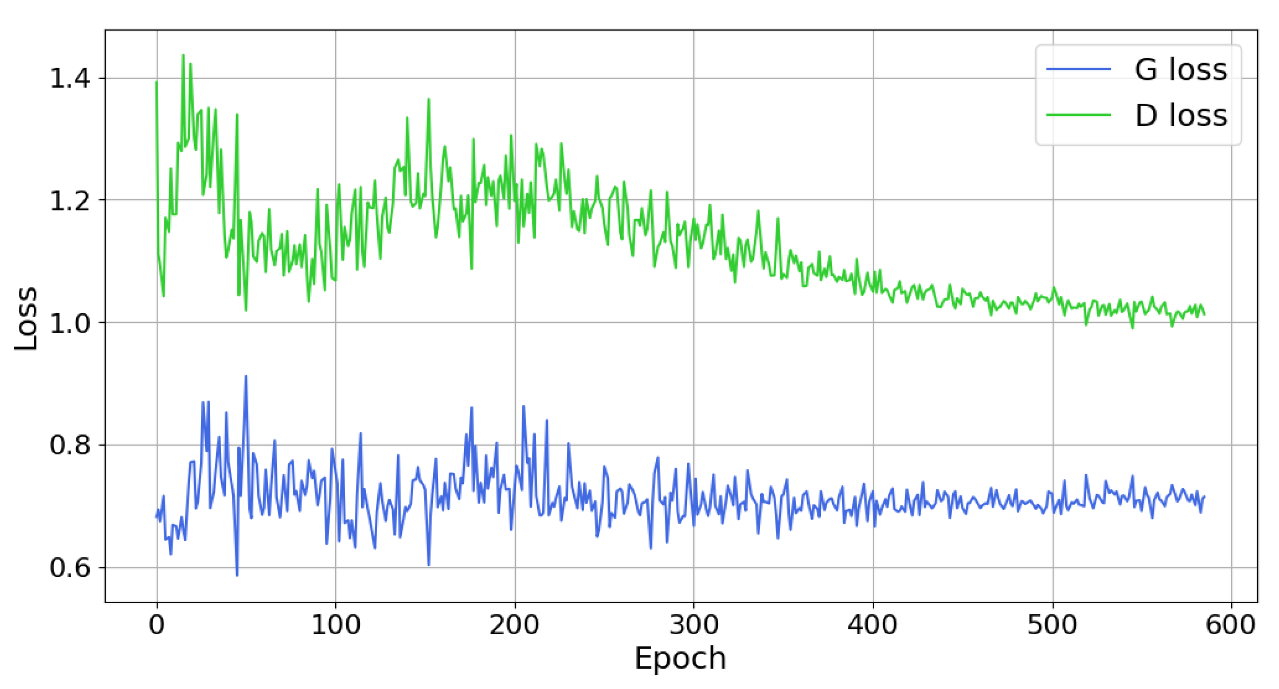
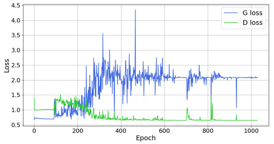
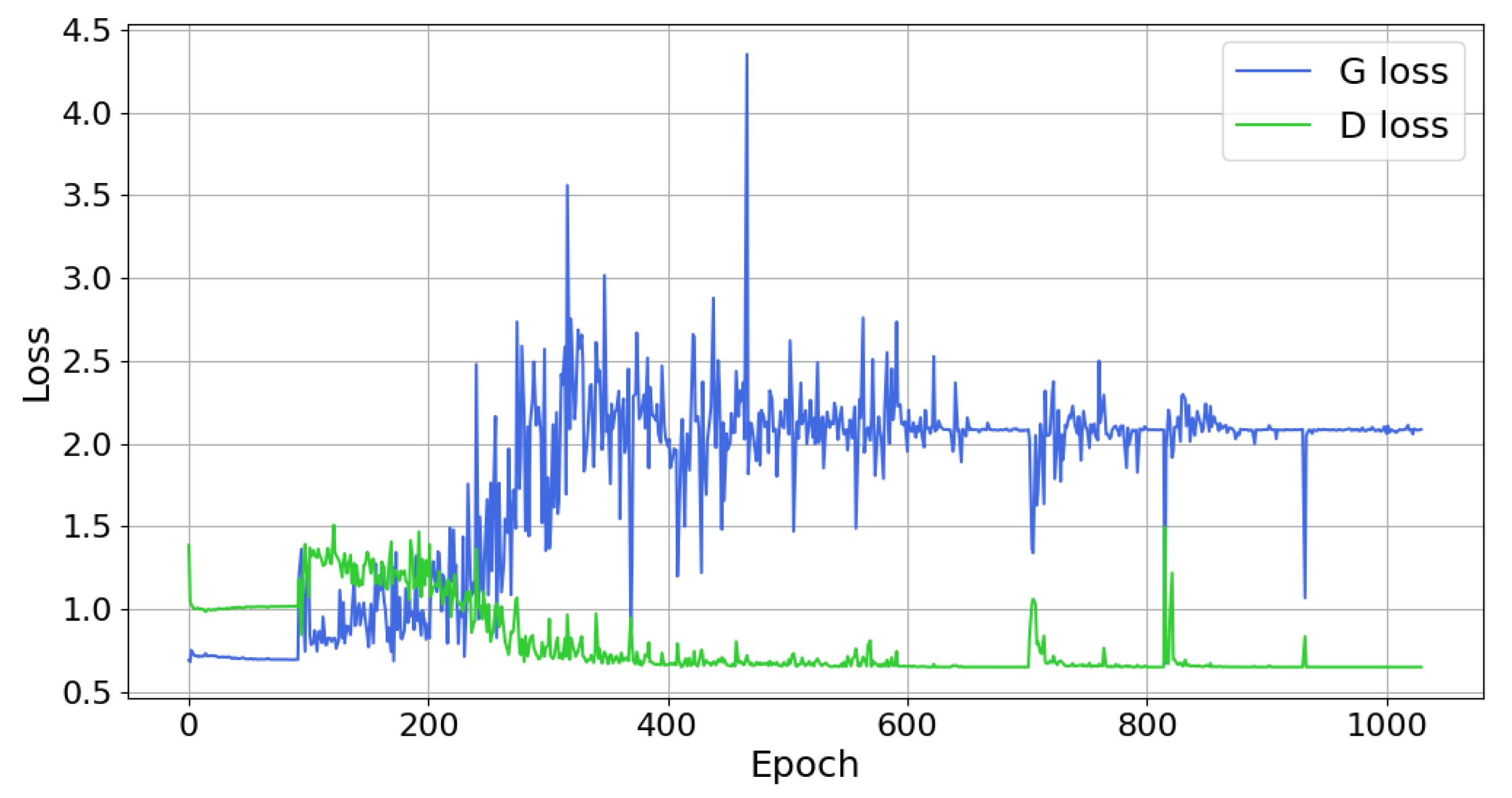
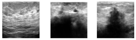
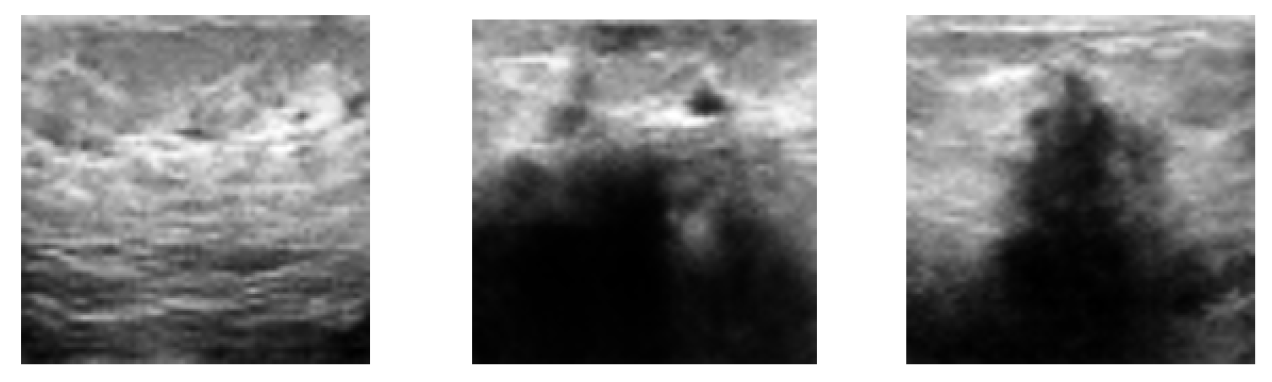
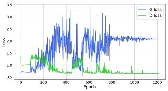
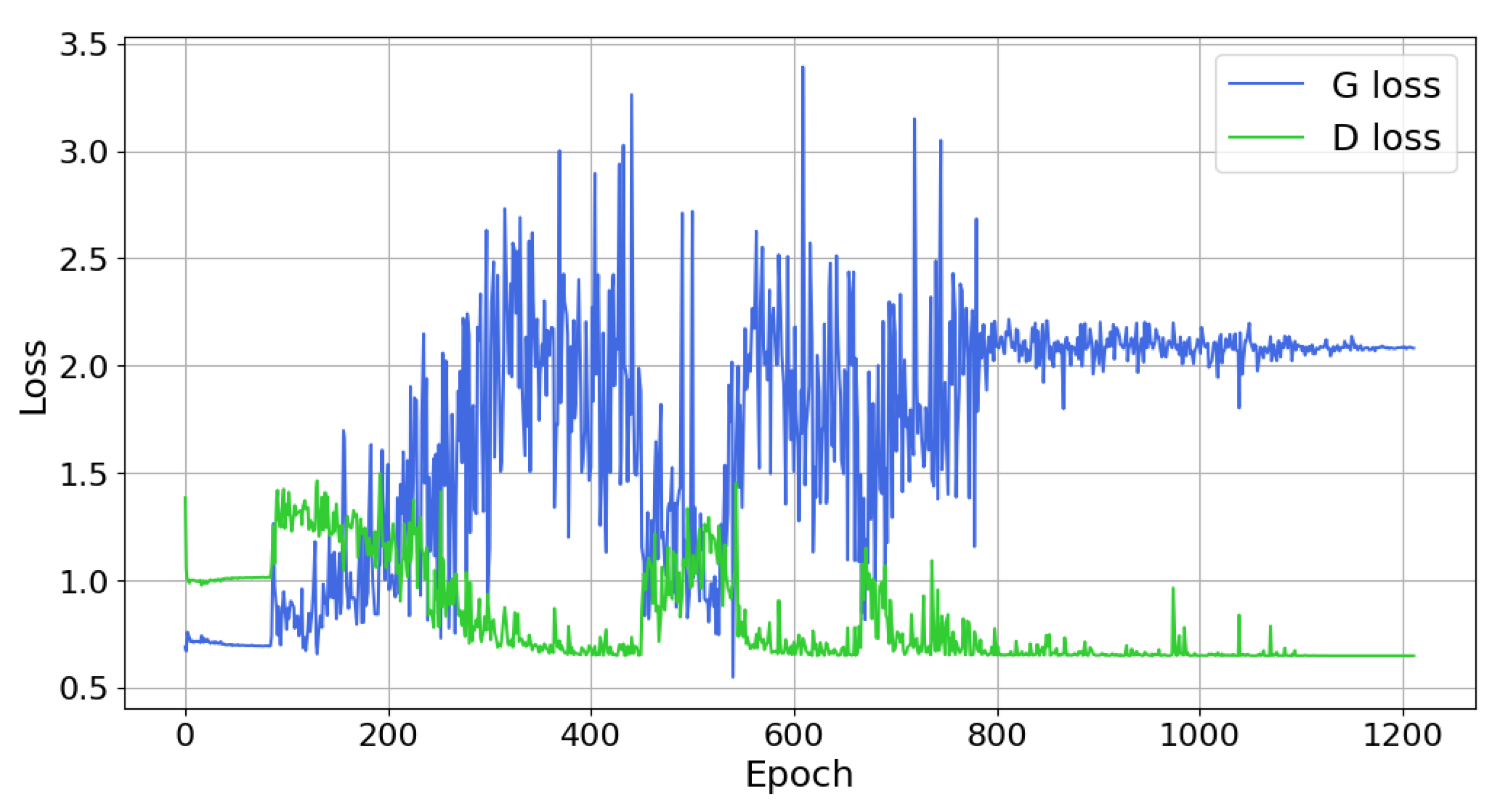
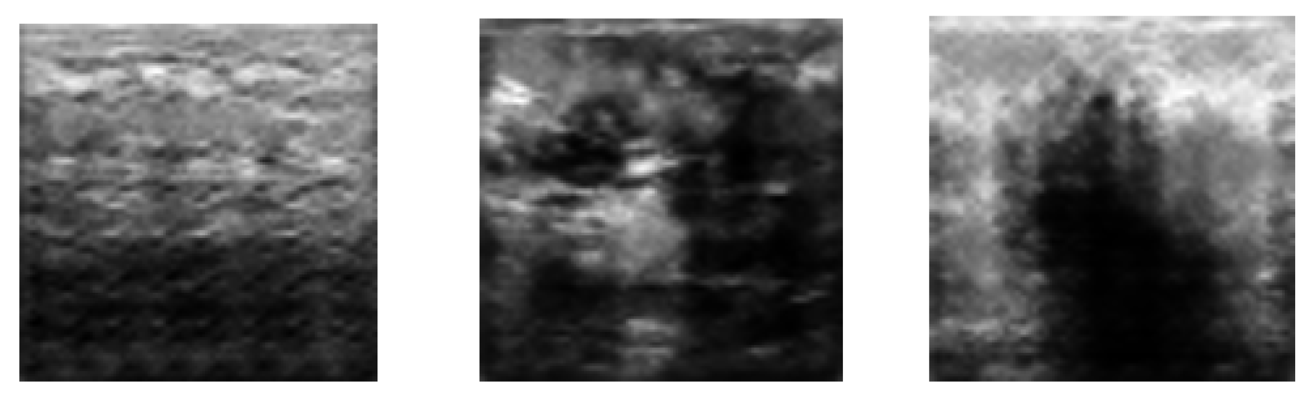
Finally, neither DCGAN nor EDCGAN guaranties the convergence of the loss function. However, the running time is limited to 2 h. The loss function may still converge given enough time. However, it might not be worth waiting 10 h to finally obtain some unrealistic images. The user interrupts training after 2 h and runs the model with a different initial image. This approach is automated, and the “impatient user algorithm” works accordingly. However, this is also a disadvantage of the model. The user does not have a guarantee that the model converges. Moreover, the postprocessing parameters (Section 9) may differ for different modalities. Some graphic illustrations of the above numerical experiments are provided below. Figure 3 shows a divergent DCGAN-SE along with examples of unsuitable images (Figure 4). However, the same model diverges in 70% of the runs and produces acceptable images (Figure 5). It is our experience that many unsuitable images can be detected by non-professionals, e.g., instructors or computer science students working on this project. However, there are many instances when the speckle noise shadows produced by the GAN appear convincing to non-professionals. Nevertheless, the structure of those synthetic images enables radiologists to detect the generated images. The convergence of the second best combination, DCGAN-SELU-SN, is shown in Figure 6. This is a preferred behavior of the loss function without hard oscillation or mode collapse.

Figure 3. Divergence. DCGAN-SE.

Figure 4. Unacceptable DCGAN-SE images.

Figure 5. Acceptable DCGAN-SE images.

Figure 6. Typical convergence of DCGAN-SELU-SN.

Finally, we offer plots of the convergence of two EDCGAN models. The loss functions converge to approximately similar limits. However, model 1 generates acceptable images, whereas model 2 fails to impress the experts. Nevertheless, the upcoming sections show that EDCGAN outperforms its competitors in several instances. The models are illustrated in Figure 7, Figure 8, Figure 9 and Figure 10. In summary, even a 100% convergence rate cannot guaranty suitable images. Moreover, suitability itself is subjective. Images suitable for one task may not be appropriate for another. However, we still consider evaluation by professionals to be important (although it is also subjective). Yet, the problem is open. There does not exist a set of synthetic (or real) images suitable for any medical processing task. The next section offers pre-processing, which is a way to tackle this issue.

Figure 7. Convergence. EDCGAN model 1.

Figure 8. Acceptable images. Model 1 (accepted).

Figure 9. Convergence. EDCGAN model 2.

Figure 10. Unacceptable images. Model 2 (rejected).

Note that the majority of competing models show convergence rates comparable with DCGAN. It could be lower by 10–15% (on this particular database), but still acceptable. However, they produce too many unrealistic images.

9. Postprocessing

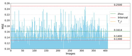
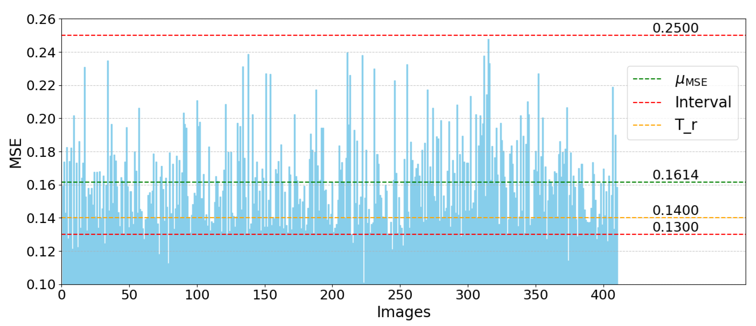
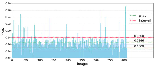
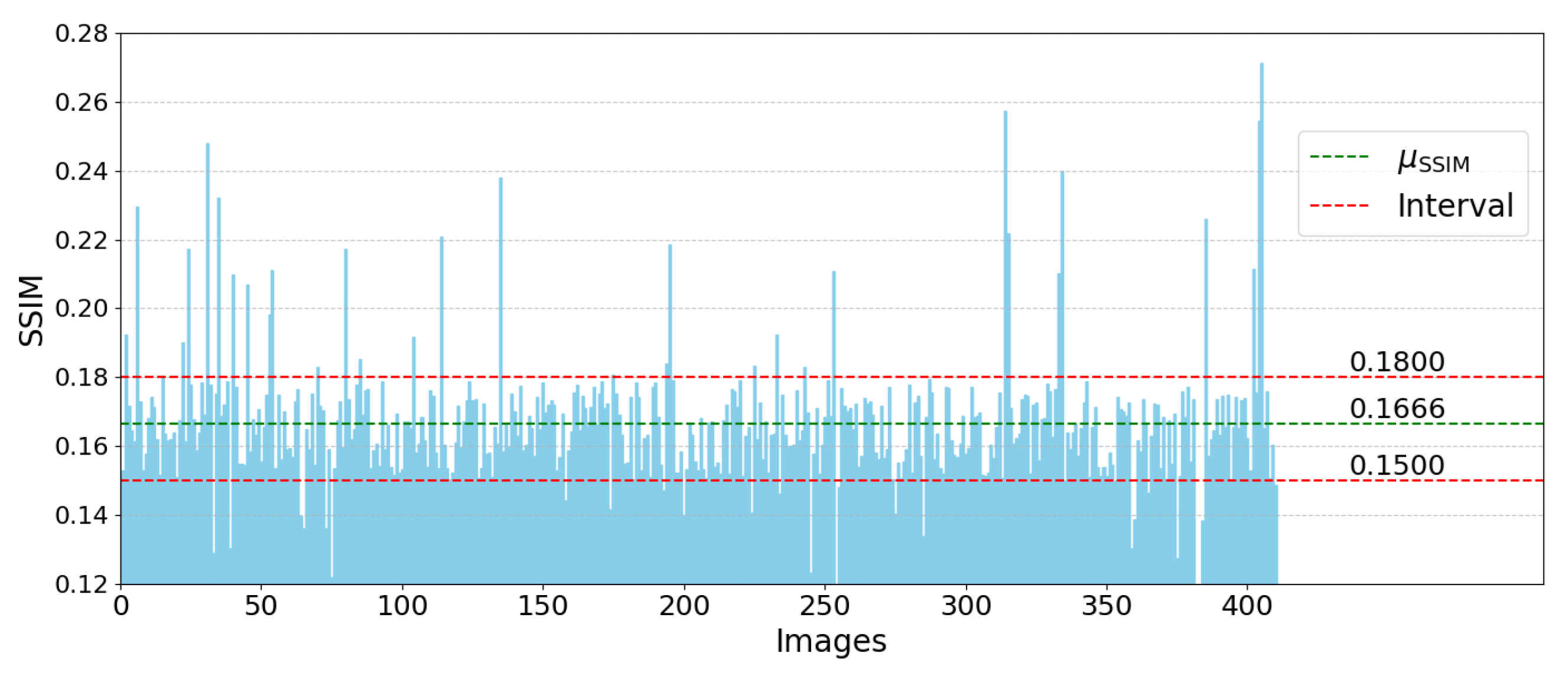
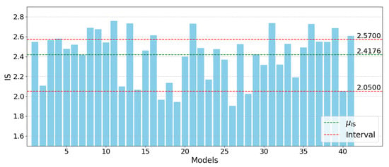
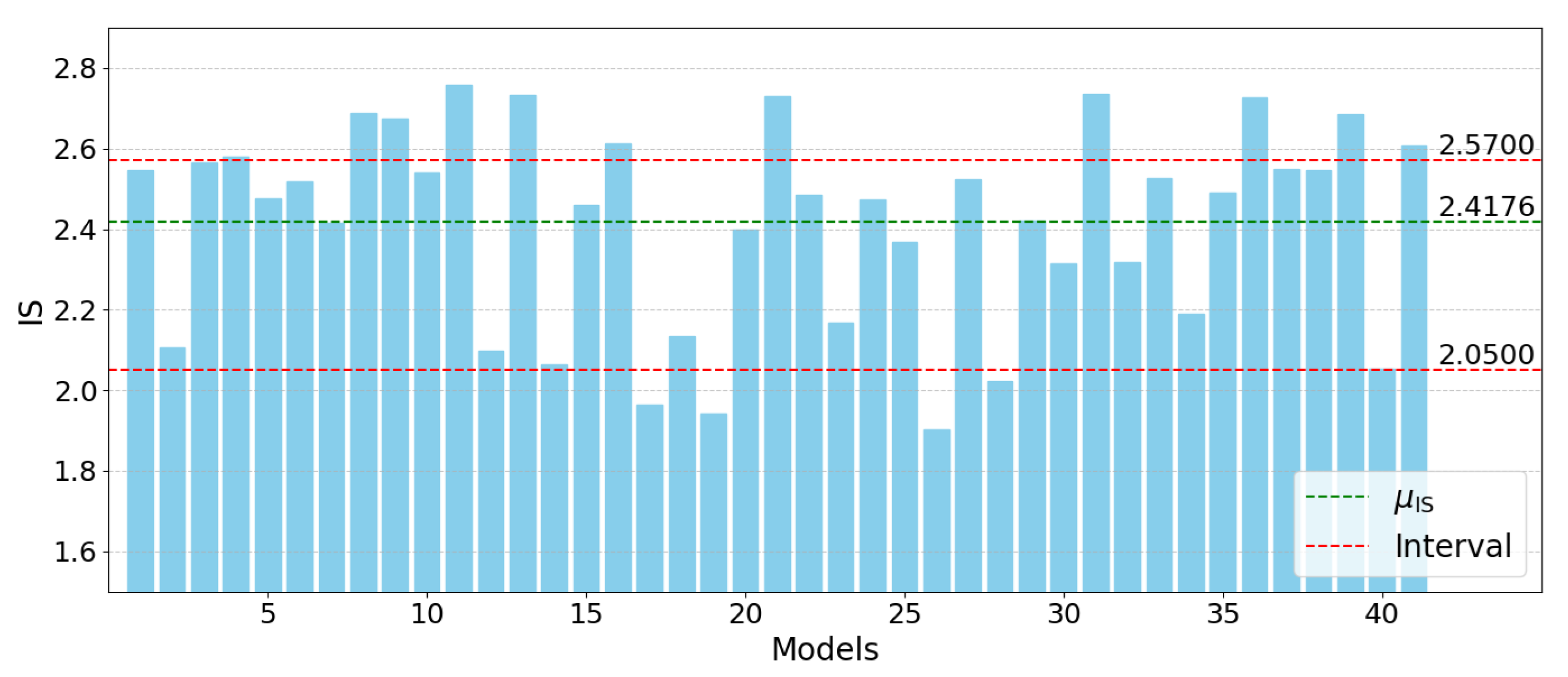
Let us analyze 50 independent, converged EDCGAN models. Each model generated 10 images. The output was evaluated visually. A total of 40 models produced acceptable images; 1 model produced both acceptable and unacceptable outputs, and 9 models failed. Figure 11, Figure 12 and Figure 13 show the results, along with the corresponding means and standard deviations.

Figure 11. Acceptable interval, MSE.

Figure 12. The acceptable interval of SSIM.

Figure 13. Acceptable interval, IS.

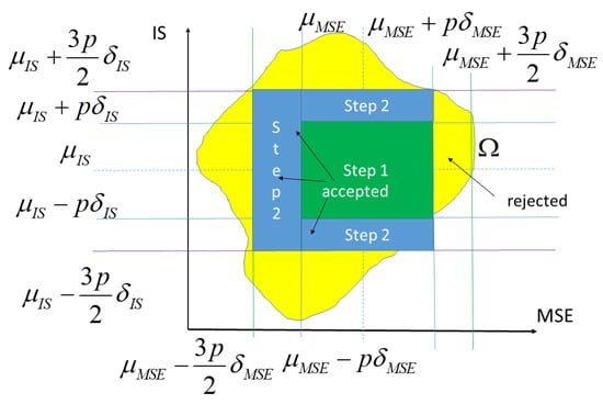
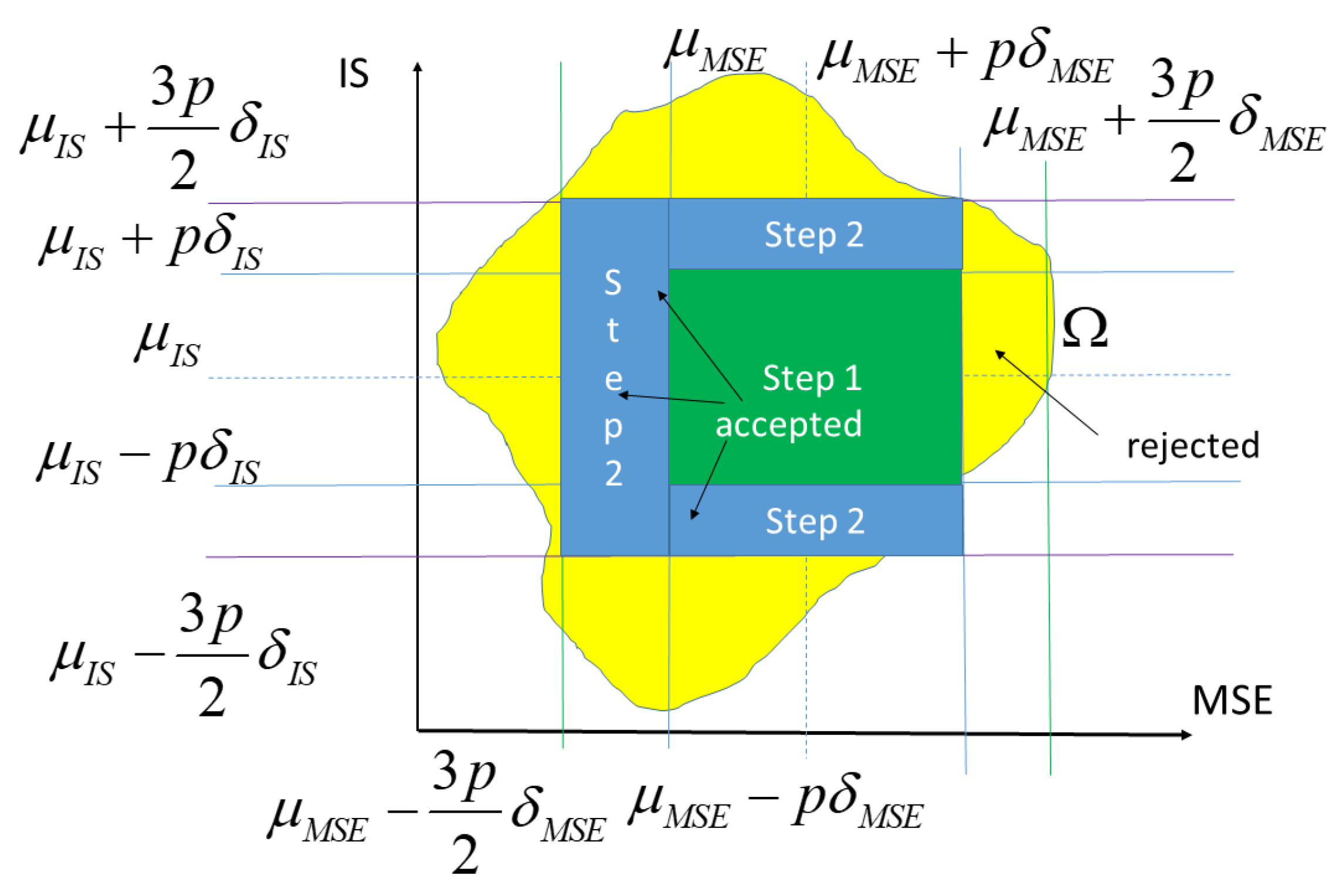
The experimental analysis (Table 3) shows that if the model produces $N_{\mathrm{crit}}\approx 5$ good images at the training stage, it usually continues to produce visually good images; however, this is not always the case. Furthermore, repetitive images must be discarded. If the model produces both good and bad images, it is retained to increase the diversity of the synthesis. The basic machine learning techniques reveal that “good fake” images must be in the interval $\mathrm{IS}\in [2.05,2.57]$, $\mathrm{SSIM}\in [0.15,0.18]$, and $\mathrm{MSE}\in [0.13,0.25]$. Additionally, the image is considered repeated if ${\mathrm{MSE}}_{min}\le T_r$, and where $T_r$ is an experimental threshold evaluated visually (Table 4). The image is compared with generated images and training images. Note that the above criteria do not guaranty that all output images are good. The thresholds for IS, SSIM and MSE have been obtained by bisection. For simplicity, Figure 14 illustrates the procedure in the two-dimensional space (MSE and IS), where the bisection step is proportional to the standard deviation $\sigma$ and p is the integer coefficient. The 3D version does not require any modifications. The procedure approximates a feasible region $\mathrm{\Sigma }$ where the number of acceptable images is more than 90%. The proportion 1/10 has been selected in order to increase the diversity of the output.

Table 3. Testing EDCGAN.

Correct models	40
Undefined models	1
# of runs for each model	100
# of images	4100
Images classified as different and “good”	1048	25.56% (of total)
Images classified as “good” visually (from 1048)	928	88.55%
Classification error		11.45%

Table 4. Hyperparameters and thresholds.

Learning rate Generator	0.0001
Learning rate Discriminator	0.0003
Batch size	8
Stopping criteria threshold	0.001
Moving average period	7
MSEmin	0.13–0.25
IS	2.05–2.57
SSIM	0.15–0.18
Repeated image threshold $T_r$	0.14

Figure 14. Two-dimensional bisection.

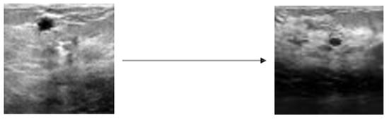
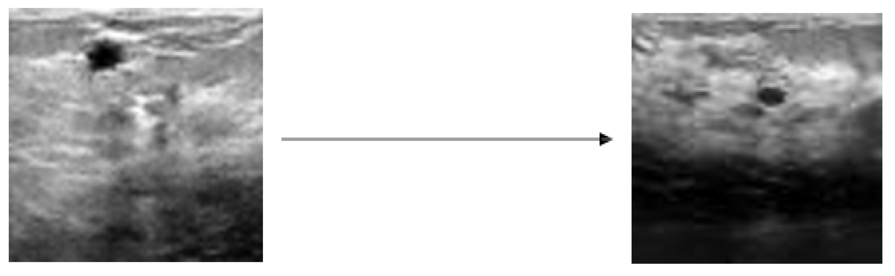
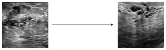
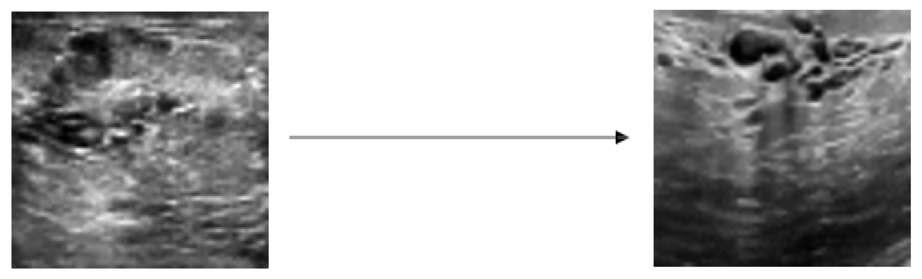
The testing stage presented below shows that the classification error does not exceed 12%. Let us initialize the input vector and produce 50 new models. This time, every model generates 100 images. The results of the experiments are shown in Table 3. The experimental hyperparameters and thresholds are illustrated and summarized in Table 4. Examples of acceptable, unacceptable, and repeated images are shown in Figure 15, Figure 16 and Figure 17. The testing results show that, contrary to the existing critique of the visual criteria, they allow us to design and postprocess the output of a basic GAN architecture to double the existing database.

Figure 15. Realistic output and the closest real image (accepted).

Figure 16. Unrealistic output (rejected).

Figure 17. Repeated image (rejected).

10. Tests Against State-of-the-Art

The performance of the EDCGAN has been evaluated using IS, SSIM, and MSE.

Quantitative Evaluation

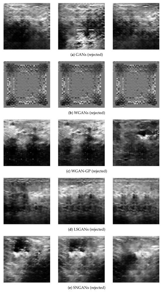
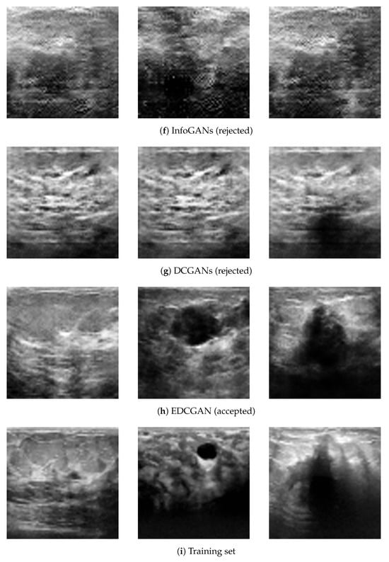
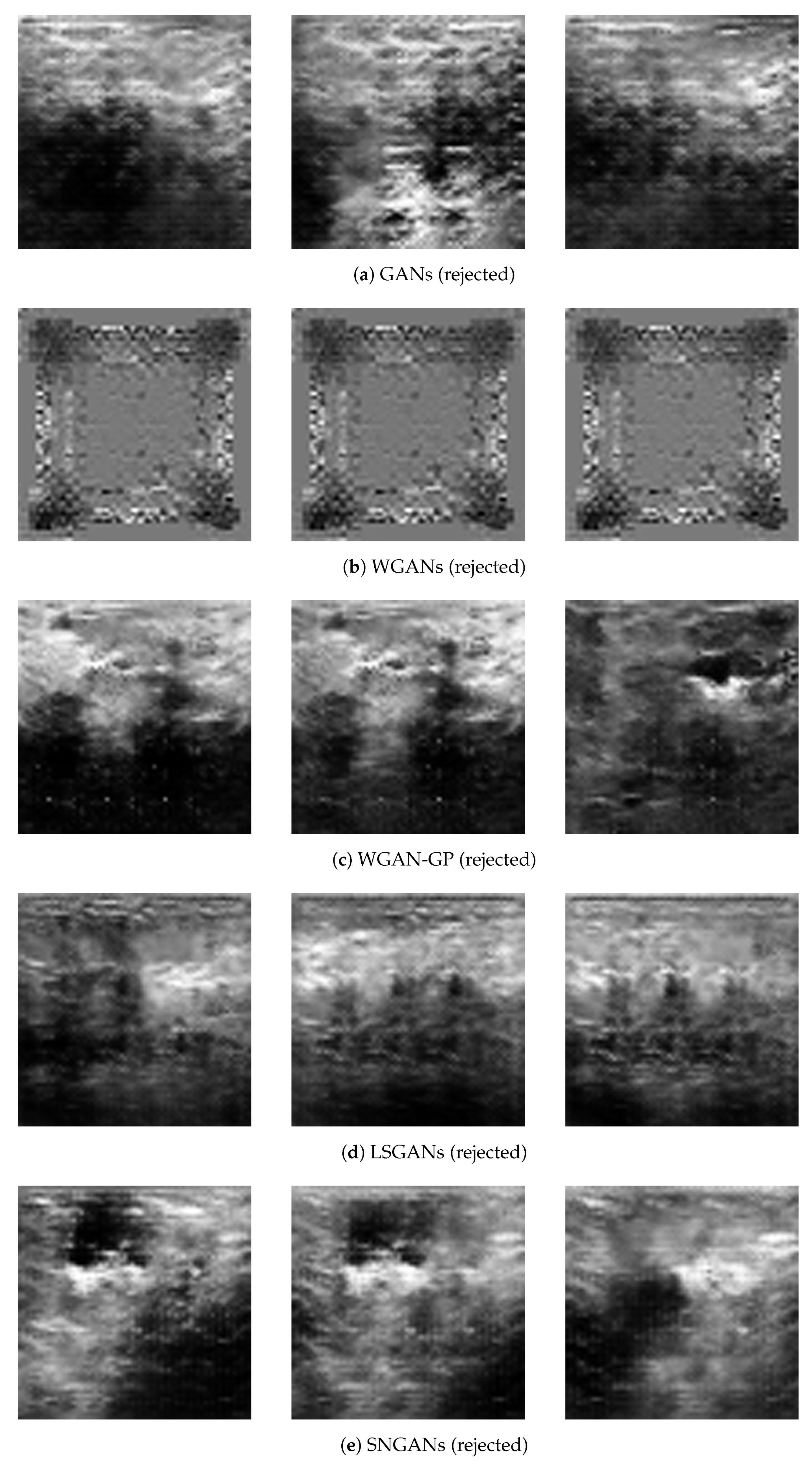
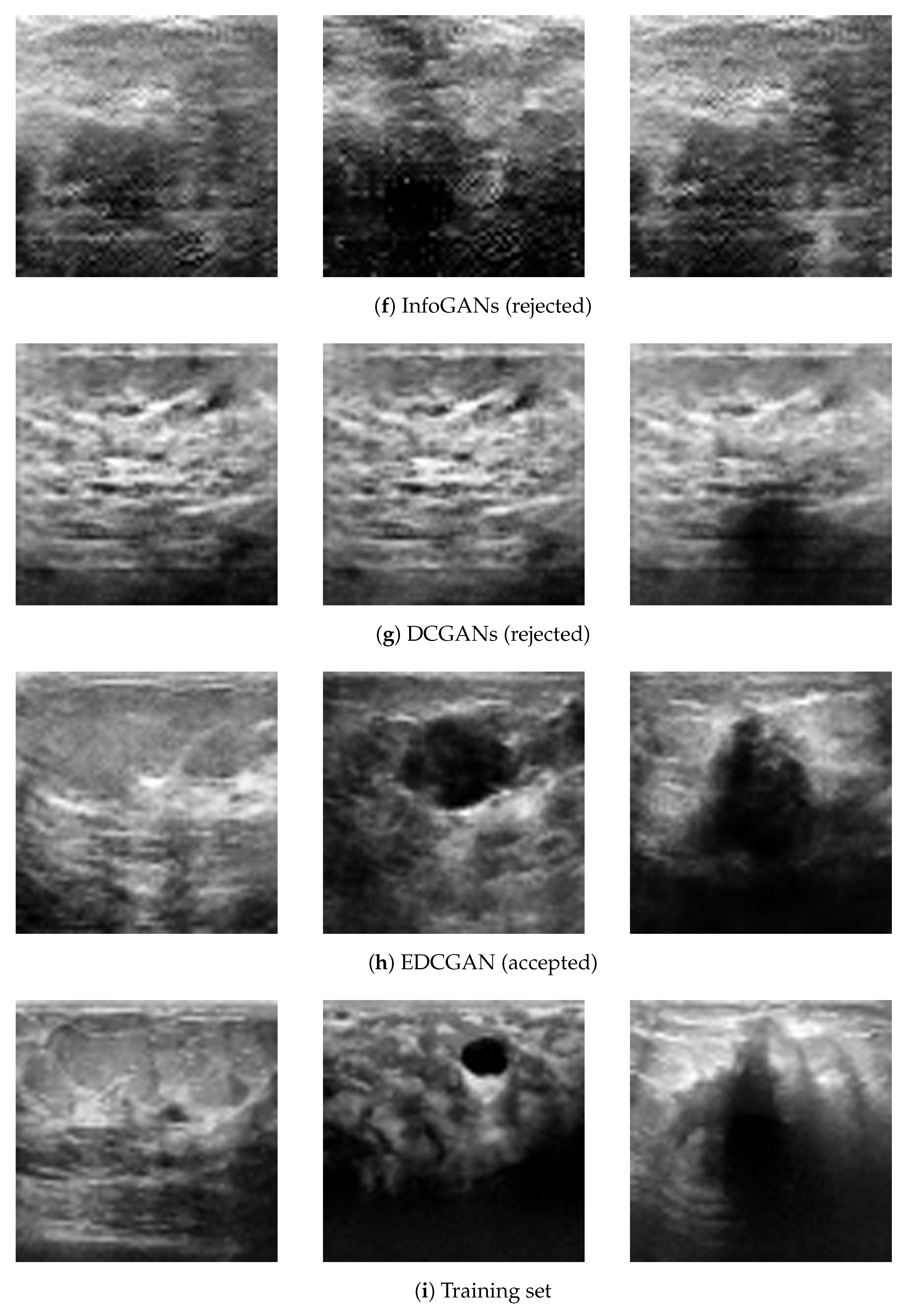
Table 5 tests the EDCGANs model against popular GAN architectures, i.e., GANs, WGANs, WGANs-GP, LSGANs, SNGANs, InfoGANs, and traditional DCGANs.

Table 5. Quality of synthetic images vs. the references and visual evaluation.

Model	IS ± Std	SSIM ± Std	MSE ± Std
GANs	1.64 ± 0.15	0.12 ± 0.01	0.26 ± 0.013
WGANs	1.52 ± 0.07	0.05 ± 0.01	0.32 ± 0.03
WGAN-GP	1.91 ± 0.16	0.10 ± 0.04	0.23 ± 0.12
LSGANs	1.89 ± 0.21	0.10 ± 0.04	0.26 ± 0.12
SNGANs	1.66 ± 0.14	0.10 ± 0.05	0.25 ± 0.09
InfoGANs	1.46 ± 0.12	0.08 ± 0.04	0.26 ± 0.11
DCGANs	1.73 ± 0.22	0.12 ± 0.016	0.23 ± 0.02
EDCGANs	2.56 ± 0.21	0.17 ± 0.013	0.17 ± 0.025
References	2.29–2.62	0.15–0.18	0.16–0.26
Radiologists	2.37	0.18	0.15

The proposed design of the algorithm shows that the synthetic images are closer to the reference models reported in the literature in terms of IS and SSIM. Namely, the average IS = 2.29–2.62 [62] obtained on 8189 images (pre-trained), SSIM = 0.18–0.15 [32]. However, MSE = 0.16–0.26 [33,63]. SSIM and IS comply with the ranges provided in the references above. The MSE is at the low end of the referenced interval. However, the reported EDCGAN range has been further substantiated by radiologists: IS = 2.3736, SSIM = 0.1811, and MSE = 0.1499.

To statistically assess the performance of EDCGAN, we compared its image-quality metrics against those of the second-best model (WGAN-GP) and the third-best model (DCGAN). Three evaluation metrics were used as follows: Inception Score (IS), Structural Similarity Index Measure (SSIM), and Mean Squared Error (MSE). For each metric, a one-tailed independent two-sample t-test with unequal variances (Welch’s t-test) was conducted using results obtained from multiple training runs. The tests were performed separately for the comparisons (i) EDCGAN vs. WGAN-GP and (ii) EDCGAN vs. DCGAN. Statistical significance was determined at the $p<0.05$ level with a sample size of $n=30$. The resulting p-values are summarized in Table 6. The results indicate that EDCGAN outperforms the competitors, being statistically significant relative to the baseline models. The results are illustrated in Figure 18.

Table 6. Statistical analysis of EDCGANs against baseline models.

Models	Metric	Goal	t-Statistic	p-Value	Result
EDCGANs vs. WGAN-GP	IS	Higher is better	4.28	<0.0001	Significant
	SSIM	Higher is better	4.29	0.0001	Significant
	MSE	Lower is better	−2.37	0.0111	Significant
EDCGANs vs. DCGAN	IS	Higher is better	6.19	<0.0001	Significant
	SSIM	Higher is better	2.74	0.0042	Significant
	MSE	Lower is better	−2.69	0.0048	Significant

Figure 18. Tests against the state-of-art.

11. Guess-the-Real-Image Game

A total of 100 images were randomly selected, consisting of 50 real images and 50 generated images. Five radiologists from two leading Hospitals of Bangkok were informed that 50% of the images were fake. This information introduced a psychological effect into the experiments; i.e., the radiologists knew that they must reject approximately half of the images shown. We consider this setting revealing, as opposed to hiding this proportion from the operators. The radiologists were blinded to the source of the images. Moreover, in their hospital settings, they used different US machines. The visual analysis was conducted on the images generated through EDCGAN vs. the competing models. The results have been averaged over the 5 observers. Table 7 and Table 8 reveal that EDCGAN produces realistic US structures and details. Radiologists were misled more frequently by EDCGAN-generated images compared to those generated by other models. The false positive rate of EDCGAN suggests that the generated images closely resemble the actual US scans. The inter-rater agreement offered by Table 7 complies with the results.

Table 7. Average confusion matrix. Visual evaluation.

Model	TP	TN	FP	FN	Ainter-rate
GANs	50.00%	40.80%	9.20%	0.00%	0.799
WGANs	50.00%	50.00%	0.00%	0.00%	1.000
WGAN-GP	50.00%	41.40%	8.60%	0.00%	0.828
LSGANs	50.00%	49.40%	0.60%	0.00%	0.988
SNGANs	50.00%	49.00%	1.00%	0.00%	0.980
InfoGANs	50.00%	49.80%	0.20%	0.00%	0.996
DCGANs	50.00%	39.40%	10.6%	0.00%	0.796
EDCGANs	31.80%	18.00%	33.00%	16.20%	0.115

Table 8. Guess-the-real-image-game results.

Model	Precision	Recall	F1 Score
GANs	0.844	1.000	0.914
WGANs	1.000	1.000	1.000
WGAN-GP	0.852	1.000	0.919
LSGANs	0.988	1.000	0.994
SNGANs	0.980	1.000	0.990
InfoGANs	0.996	1.000	0.998
DCGANs	0.826	1.000	0.904
EDCGANs	0.491	0.663	0.563

Many competing images include small artifacts that allow experts to detect artificial images. However, this does not necessarily mean that they are inappropriate for training AI models. The above is an open problem and is a subject of ongoing discussion outside the scope of this paper. Furthermore, the radiologists noticed that the images generated by the ECGAN were difficult to detect. They knew that half of the images were synthetic. Hence, they admitted that it was often a random guess rather than a confident opinion. In the case of the proposed model, TP is approximately equal to FP, and TN is approximately equal to FN, whereas the experts classified images produced by the competing models with almost 100% accuracy. On average, 66% of the fake EDCGAN images (33% of the total number of images) were considered real. The best result is 82% of the fake images. However, the high percentage of FP relative to FP+TN indicates the efficiency of the proposed scheme, given that the competing models are unable to deceive the experts. Furthermore, FN = 16.2% contributes to the credibility of EDCGAN, proving that the experts were actually uncertain about the source of these images. This is also indicated by A_inter-rate in Table 7 [64]. We reiterate that the synthetic images that have been correctly classified as fake by humans are not necessarily detrimental to training. This has been demonstrated by the classification model in the upcoming chapter. However, EDCGAN was able to improve the classification rate of the pre-trained Res18-Net.

12. Application to Classification of the US Images

Transfer learning is a popular strategy for medical image analysis, allowing the leveraging of models pre-trained on large natural image datasets to improve the performance of specialized medical AI systems. The benefits include reducing training time and skipping difficult stages in developing a DL medical system from scratch. This section demonstrates the transfer of a pre-trained model to the medical classification task, applying the model to a small database and showing the efficiency of augmenting the small dataset using EDCGAN. In order to evaluate the efficiency of the generated images, a DL model based on ResNet-18 was used [2]. The model has been pre-trained on ImageNet1K, which covers 1000 categories and includes 1.28 million samples. The model was modified to classify US images into benign and malignant tumors or healthy breast tissue.

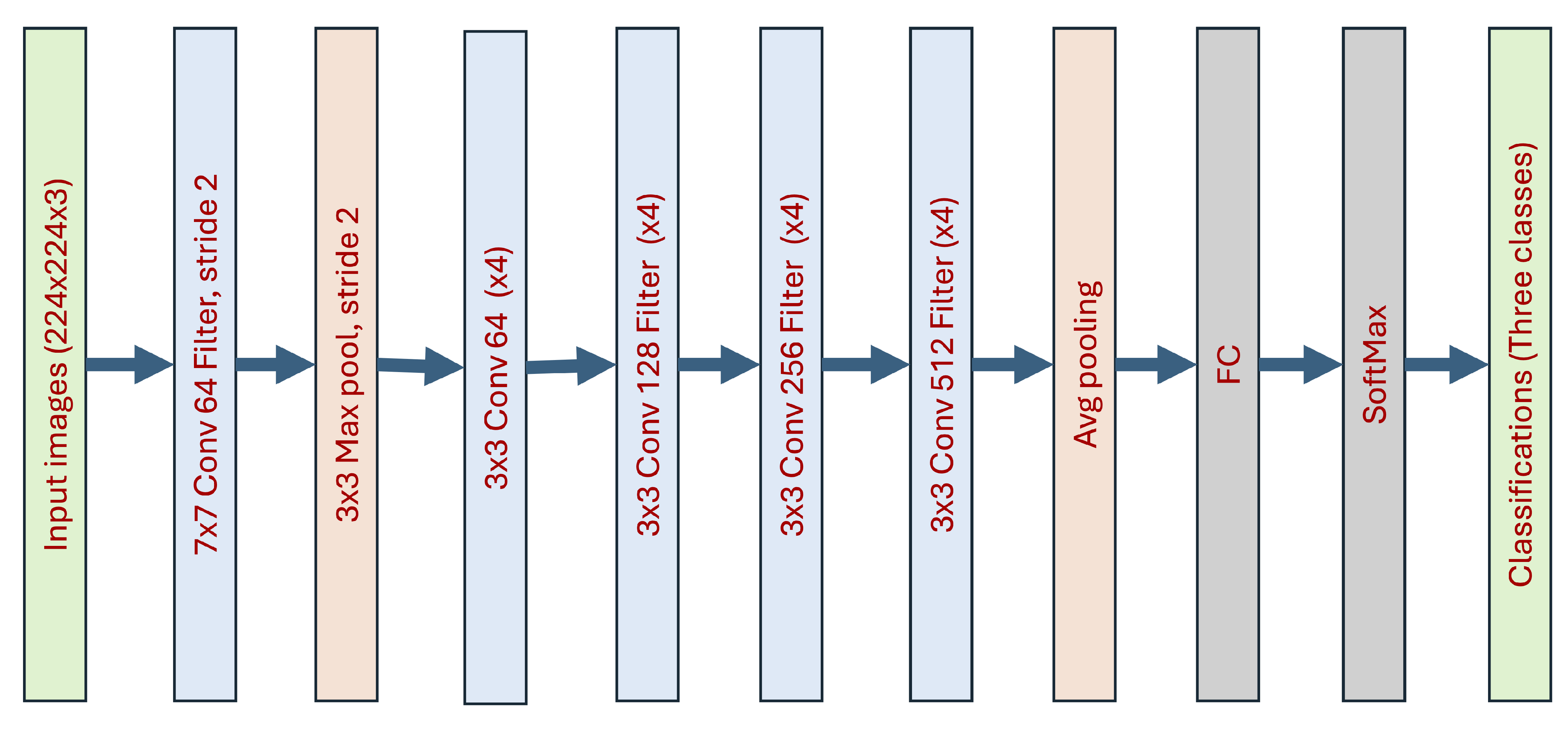
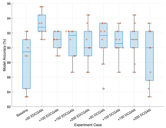
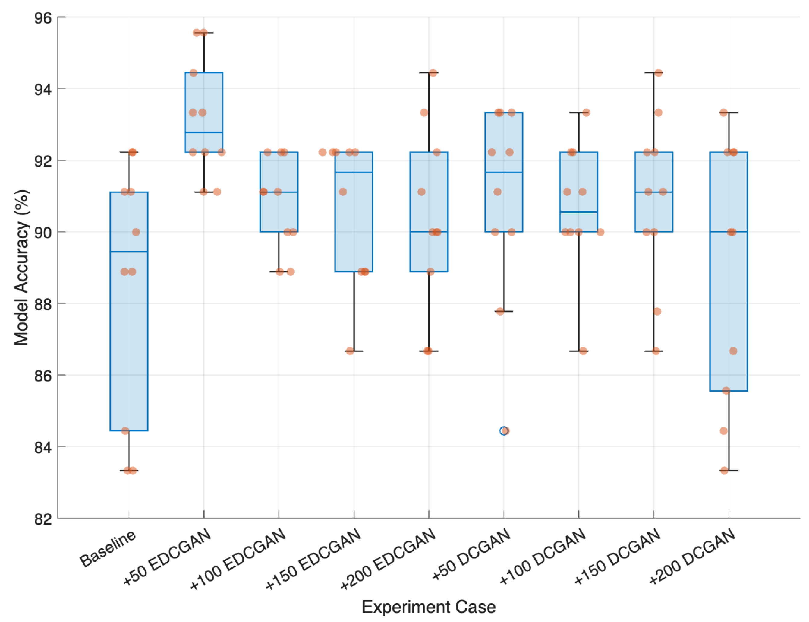
The architecture of the classification model is shown in Figure 19. The testing dataset remained fixed, consisting of 30 images per class for a total of 90 images. The base training dataset comprises 100 real images per class, randomly selected from the dataset and kept constant across experimental conditions. For each training run, the dataset was partitioned with an 80:20 ratio for training and validation. Synthetic images generated by EDCGAN and DCGAN were subsequently added exclusively to the training dataset, with the number of added images set to 50, 100, 150, and 200 per class. The transfer learning model was trained for 150 epochs, and each experimental configuration was repeated ten times. The results are summarized in Table 9. To determine whether adding synthetic images to the training dataset leads to a statistically significant improvement in classification performance, an independent two-sample t-test with unequal variances (Welch’s t-test) was conducted. For each experimental condition, the accuracies from ten training runs were compared against those from the baseline experiments (without synthetic images). Statistically significant runs are indicated in Table 9 by the boldface and the asterisk (see also the whiskers in Figure 20). Hence, the images generated by EDCGAN improve the efficiency of the pre-trained ResNet18 and outperform the competing DCGAN.

Figure 19. The transfer learning model based on ResNet-18 architecture [2].

Table 9. Tests against DCGAN (* denotes statistical significance).

Method	Class	Real Img.	Synthetic Img.	Accuracy (%)	Precision	Sensitivity (Recall)	Specificity	F1 Score (Dice)	Jaccard
Base	Normal	100	0	88.56	0.94	0.84	0.87	0.97	0.80
	Benign	100	0		0.89	0.96	0.92	0.94	0.86
	Malignant	100	0		0.83	0.86	0.84	0.91	0.73
EDCGAN Synthetic Images	Normal	100	25	92.89 *	0.94	0.84	0.89	0.97	0.80
	Benign	100	25		0.89	0.96	0.92	0.94	0.86
	Malignant	100	25		0.83	0.86	0.84	0.91	0.73
	Normal	100	50	93.11 *	0.98	0.92	0.95	0.99	0.90
	Benign	100	50		0.91	0.96	0.93	0.95	0.88
	Malignant	100	50		0.91	0.92	0.91	0.96	0.84
	Normal	100	100	90.78	0.99	0.86	0.92	0.99	0.85
	Benign	100	100		0.89	0.95	0.92	0.94	0.86
	Malignant	100	100		0.86	0.91	0.88	0.92	0.79
	Normal	100	150	90.56	0.95	0.92	0.93	0.98	0.88
	Benign	100	150		0.87	0.93	0.90	0.93	0.82
	Malignant	100	150		0.89	0.87	0.88	0.95	0.79
	Normal	100	200	90.33	0.97	0.87	0.92	0.99	0.85
	Benign	100	200		0.89	0.94	0.92	0.95	0.85
	Malignant	100	200		0.86	0.90	0.88	0.92	0.78
DCGAN Synthetic Images	Normal	100	25	90.56	0.96	0.88	0.92	0.98	0.85
	Benign	100	25		0.89	0.96	0.92	0.94	0.86
	Malignant	100	25		0.87	0.88	0.87	0.93	0.78
	Normal	100	50	90.78	0.94	0.90	0.92	0.97	0.86
	Benign	100	50		0.90	0.94	0.92	0.95	0.85
	Malignant	100	50		0.88	0.89	0.88	0.94	0.79
	Normal	100	100	90.67	0.95	0.88	0.91	0.98	0.84
	Benign	100	100		0.89	0.96	0.93	0.94	0.86
	Malignant	100	100		0.88	0.88	0.88	0.94	0.79
	Normal	100	150	90.89	0.96	0.89	0.92	0.98	0.86
	Benign	100	150		0.88	0.95	0.91	0.94	0.84
	Malignant	100	150		0.89	0.89	0.89	0.94	0.80
	Normal	100	200	89.00	0.95	0.85	0.89	0.98	0.81
	Benign	100	200		0.87	0.95	0.91	0.93	0.84
	Malignant	100	200		0.86	0.87	0.86	0.93	0.76

Figure 20. Improvement with synthetic images.

13. Discussion: Limitations and Future Research

Despite the promising results obtained from the evaluation of the radiologists and the augmentation of real classification, the proposed scheme is specific to BUS images. Moreover, it is specific to the particular database where the convergence of the loss function is not 100% reliable. That is why the proposed postprocessing is based on supervised ML to establish proper thresholds for images produced by converged models. The thresholds depend on the training dataset and may vary when the dataset is changed or even increased. However, it is a practical approach to establishing a suitable Generator. It can be easily replicated using a small startup dataset and a relatively short time spent with radiologists. Nevertheless, more studies should analyze the applicability of the model to other databases and even to other US imaging modalities, such as prostate and thyroid glands, and even the fusion of MRI and US. Augmenting other existing pre-trained models is another promising research direction. At the top level of the analysis of such models is the model-dependent suitability of produced images for training. Images suitable for one task may not be appropriate for another. However, we still consider evaluation by professionals to be important, although it is also subjective. The problem is open and lies outside the scope of the paper. The second top-level direction is integration into particular downstream tasks and the combination of supervised, semi-supervised, and unsupervised systems.

14. Conclusions

The proposed EDCGAN model generates suitable BUS images using a small initial dataset. The combination of SN, SE-block, SELU, and postprocessing improves the quality of the synthetic images. The ML classifier, based on standard metrics and a visual assessment by radiologists, supports the above claim. In particular, visually sound synthetic images selected by radiologists are suitable for training and can be used as a basis to construct an appropriate classifier. The efficiency of the proposed models has been supported by the innovative guess-the-real-image game and successive augmentation of pre-trained ResNet18.

References

- World Health Organization. Breast Cancer. Available online: https://www.who.int/news-room/fact-sheets/detail/breast-cancer (accessed on 14 January 2025).
- He, K.; Zhang, X.; Ren, S.; Sun, J. Deep residual learning for image recognition. In Proceedings of the IEEE Conference on Computer Vision and Pattern Recognition, Las Vegas, NV, USA, 27–30 June 2016; pp. 770–778. [Google Scholar]
- Upadhyay, A.K.; Bhandari, A.K. Advances in deep learning models for resolving medical image segmentation data scarcity problem: A topical review. Arch. Comput. Methods Eng. 2024, 31, 1701–1719. [Google Scholar]
- Gonzales Martinez, R.; van Dongen, D.M. Deep learning algorithms for the early detection of breast cancer: A comparative study with traditional machine learning. Inform. Med. Unlocked 2023, 41, 101317. [Google Scholar] [CrossRef] [Scilit]
- LeCun, Y.; Bengio, Y.; Hinton, G. Deep learning. Nature 2015, 521, 436–444. [Google Scholar] [CrossRef] [Scilit]
- Tupper, A.; Gagné, C. Revisiting Data Augmentation for Ultrasound Images. arXiv 2025, arXiv:2501.13193. [Google Scholar] [CrossRef] [Scilit]
- Goodfellow, I.; Pouget-Abadie, J.; Mirza, M.; Xu, B.; Warde-Farley, D.; Ozair, S.; Courville, A.; Bengio, Y. Generative adversarial nets. In Proceedings of the 27th International Conference on Neural Information Processing Systems, Montreal, QC, Canada, 8–13 December 2014; Volume 2, pp. 2672–2680. [Google Scholar]
- Chen, Y.; Yang, X.H.; Wei, Z.; Heidari, A.A.; Zheng, N.; Li, Z.; Chen, H.; Hu, H.; Zhou, Q.; Guan, Q. Generative adversarial networks in medical image augmentation: A review. Comput. Biol. Med. 2022, 144, 105382. [Google Scholar] [CrossRef] [Scilit] [PubMed]
- Kumar, V.; Sharma, N.M.; Mahapatra, P.K.; Dogra, N.; Maurya, L.; Ahmad, F.; Panda, P. Enhancing Left Ventricular Segmentation in Echocardiograms Through GAN-Based Synthetic Data Augmentation and MultiResUNet Architecture. Diagnostics 2025, 15, 663. [Google Scholar] [CrossRef] [Scilit]
- Karras, T.; Aittala, M.; Hellsten, J.; Laine, S.; Lehtinen, J.; Aila, T. Training generative adversarial networks with limited data. In Proceedings of the 34th International Conference on Neural Information Processing Systems, Vancouver, BC, Canada, 6–12 December 2020; pp. 12104–12114. [Google Scholar]
- Latif, J.; Xiao, C.; Imran, A.; Tu, S. Medical imaging using machine learning and deep learning algorithms: A review. In Proceedings of the 2019 2nd International Conference on Computing, Mathematics and Engineering Technologies (iCoMET), Sukkur, Pakistan, 30–31 January 2019; IEEE: New York, NY, USA; pp. 1–5. [Google Scholar]
- Wang, E.K.; Chen, C.M.; Hassan, M.M.; Almogren, A. A deep learning based medical image segmentation technique in Internet-of-Medical-Things domain. Future Gener. Comput. Syst. 2020, 108, 135–144. [Google Scholar]
- Wang, S.; Yang, D.M.; Rong, R.; Zhan, X.; Xiao, G. Pathology image analysis using segmentation deep learning algorithms. Am. J. Pathol. 2019, 189, 1686–1698. [Google Scholar] [CrossRef] [Scilit]
- Razzak, M.I.; Naz, S.; Zaib, A. Deep learning for medical image processing: Overview, challenges and the future. Classif. Bioapps Autom. Decis. Mak. 2017, 26, 323–350. [Google Scholar] [CrossRef] [Scilit]
- Zhang, Y.; Gorriz, J.M.; Dong, Z. Deep learning in medical image analysis. J. Imaging 2021, 7, 74. [Google Scholar] [CrossRef] [Scilit]
- Ker, J.; Wang, L.; Rao, J.; Lim, T. Deep learning applications in medical image analysis. IEEE Access 2017, 6, 9375–9389. [Google Scholar] [CrossRef] [Scilit]
- Tang, Y.; Cai, J.; Lu, L.; Harrison, A.P.; Yan, K.; Xiao, J.; Yang, L.; Summers, R.M. CT image enhancement using stacked generative adversarial networks and transfer learning for lesion segmentation improvement. In Machine Learning in Medical Imaging; Springer: Cham, Switzerland, 2018; pp. 46–54. [Google Scholar]
- Oktay, O.; Ferrante, E.; Kamnitsas, K.; Heinrich, M.; Bai, W.; Caballero, J.; Cook, S.A.; De Marvao, A.; Dawes, T.; O‘Regan, D.P.; et al. Anatomically constrained neural networks (ACNNs): Application to cardiac image enhancement and segmentation. IEEE Trans. Med. Imaging 2017, 37, 384–395. [Google Scholar] [CrossRef] [Scilit]
- Zhu, J.; Tan, C.; Yang, J.; Yang, G.; Lio’, P. Arbitrary scale super-resolution for medical images. Int. J. Neural Syst. 2021, 31, 2150037. [Google Scholar] [CrossRef] [Scilit]
- Ma, Y.; Liu, K.; Xiong, H.; Fang, P.; Li, X.; Chen, Y.; Yan, Z.; Zhou, Z.; Liu, C. Medical image super-resolution using a relativistic average generative adversarial network. Nucl. Instruments Methods Phys. Res. Sect. A Accel. Spectrometers Detect. Assoc. Equip. 2021, 992, 165053. [Google Scholar] [CrossRef] [Scilit]
- Xia, Y.; Ravikumar, N.; Greenwood, J.P.; Neubauer, S.; Petersen, S.E.; Frangi, A.F. Super-resolution of cardiac MR cine imaging using conditional GANs and unsupervised transfer learning. Med. Image Anal. 2021, 71, 102037. [Google Scholar] [CrossRef] [Scilit]
- Liu, H.; Hu, D.; Li, H.; Oguz, I. Medical Image Segmentation Using Deep Learning. In Deep Learning in Healthcare: Paradigms and Applications; Springer International Publishing: Cham, Switzerland, 2020; pp. 17–31. [Google Scholar]
- Upadhyay, A.K.; Bhandari, A.K. hlSemi-Supervised Modified-UNet for Lung Infection Image Segmentation. IEEE Trans. Radiat. Plasma Med. Sci. 2023, 7, 638–649. [Google Scholar] [CrossRef] [Scilit]
- Teng, Q.; Liu, Z.; Song, Y.; Han, K.; Lu, Y. A survey on the interpretability of deep learning in medical diagnosis. Multimed. Syst. 2022, 28, 2335–2355. [Google Scholar] [CrossRef] [Scilit]
- Karunanayake, N.; Makhanov, S.S. When deep learning is not enough: Artificial life as a supplementary tool for segmentation of ultrasound images of breast cancer. Med. Biol. Eng. Comput. 2025, 63, 2497–2520. [Google Scholar] [CrossRef] [Scilit] [PubMed]
- Zhang, J.; Wu, X.; Liu, S.; Fan, Y.; Chen, Y.; Lyu, G.; He, S. Adaptive batch-fusion self-supervised learning for ultrasound image pretraining. Comput. Med. Imaging Graph. 2025, 124, 102599. [Google Scholar] [CrossRef] [Scilit]
- Mohammed, A.A.; Geng, X.; Wang, J.; Fateh, A.A.; Hassan, M.; Ali, Z. SSL-OHE: A self-supervised ensemble approach for early diagnosis of biliary atresia from sonographic images. Biomed. Signal Process. Control 2026, 112, 108539. [Google Scholar] [CrossRef] [Scilit]
- Yoon, J.T.; Lee, K.M.; Oh, J.H.; Kim, H.G.; Jeong, J.W. Insights and considerations in development and performance evaluation of generative adversarial networks (GANs): What radiologists need to know. Diagnostics 2024, 14, 1756. [Google Scholar] [CrossRef] [Scilit] [PubMed]
- Zhu, J.Y.; Park, T.; Isola, P.; Efros, A.A. Unpaired image-to-image translation using cycle-consistent adversarial networks. In Proceedings of the IEEE International Conference on Computer Vision (ICCV), Venice, Italy, 22–29 October 2017; pp. 2223–2232. [Google Scholar]
- Sille, R.; Choudhury, T.; Sharma, A.; Chauhan, P.; Tomar, R.; Sharma, D. A novel generative adversarial network-based approach for automated brain tumour segmentation. Medicina 2023, 59, 10119. [Google Scholar] [CrossRef] [Scilit]
- Fujioka, T.; Mori, M.; Kubota, K.; Kikuchi, Y.; Katsuta, L.; Adachi, M.; Oda, G.; Nakagawa, T.; Kitazume, Y.; Tateishi, U. Breast ultrasound image synthesis using deep convolutional generative adversarial networks. Diagnostics 2019, 9, 176. [Google Scholar] [CrossRef] [Scilit]
- Maack, L.; Holstein, L.; Schlaefer, A. GANs for generation of synthetic ultrasound images from small datasets. Comput. Digit. Biol. 2022, 5, 17–25. [Google Scholar] [CrossRef] [Scilit]
- Kumar, D.; Mehta, M.A.; Chatterjee, I. Empirical analysis of deep convolutional generative adversarial network for ultrasound image synthesis. Open Biomed. Eng. J. 2021, 15, 71–77. [Google Scholar] [CrossRef] [Scilit]
- Atri, H.; Shadi, M.; Sargolzaei, M. Generating synthetic medical images with limited data using auxiliary classifier generative adversarial network: A study on thyroid ultrasound images. J. Ultrasound 2024, 27, 105–121. [Google Scholar]
- Radford, A.; Metz, L.; Chintala, S. Unsupervised representation learning with deep convolutional generative adversarial networks. arXiv 2016, arXiv:1511.06434. [Google Scholar] [CrossRef] [Scilit]
- Skandarani, Y.; Jodoin, P.M.; Lalande, A. GANs for medical image synthesis: An empirical study. J. Imaging 2023, 9, 69. [Google Scholar] [CrossRef] [Scilit] [PubMed]
- Arjovsky, M.; Chintala, S.; Bottou, L. Wasserstein GAN. arXiv 2017, arXiv:1701.07875. [Google Scholar]
- Gulrajani, I.; Ahmed, F.; Arjovsky, M.; Dumoulin, V.; Courville, A.C. Improved training of Wasserstein GANs. Adv. Neural Inf. Process. Syst. 2017, 30, 5767–5777. [Google Scholar]
- Kossale, Y.; Airaj, M.; Darouichi, A. Mode collapse in generative adversarial networks: An overview. In Proceedings of the 2022 8th International Conference on Optimization and Applications (ICOA), Sestri Levante, Italy, 6–7 October 2022; pp. 1–6. [Google Scholar] [CrossRef] [Scilit]
- Mao, X.; Li, Q.; Xie, H.; Lau, R.Y.; Wang, Z.; Smolley, P.S. Least squares generative adversarial networks. In Proceedings of the IEEE International Conference on Computer Vision (ICCV), Venice, Italy, 22–29 October 2017; pp. 2794–2802. [Google Scholar]
- Miyato, T.; Kataoka, T.; Koyama, M.; Ishii, S. Spectral normalization for generative adversarial networks. arXiv 2018, arXiv:1802.05957. [Google Scholar] [CrossRef] [Scilit]
- Chen, X.; Duan, Y.; Houthooft, R.; Schulman, J.; Sutskever, I.; Abbeel, P. InfoGAN: Interpretable representation learning by information maximizing generative adversarial nets. Adv. Neural Inf. Process. Syst. 2016, 29, 2172–2180. [Google Scholar]
- Hu, J.; Shen, L.; Sun, G. Squeeze-and-excitation networks. In Proceedings of the IEEE Conference on Computer Vision and Pattern Recognition, Salt Lake City, UT, USA, 18–23 June 2018; pp. 7132–7141. [Google Scholar]
- Klambauer, G.; Unterthiner, T.; Mayr, A.; Hochreiter, S. Self-normalizing neural networks. Adv. Neural Inf. Process. Syst. 2017, 30. [Google Scholar]
- Müller, R.; Kornblith, S.; Hinton, G.E. When does label smoothing help? Adv. Neural Inf. Process. Syst. 2019, 32. [Google Scholar]
- Al-Dhabyani, W.; Gomaa, M.; Khaled, H.; Fahmy, A. Dataset of breast ultrasound images. Data Brief 2020, 28, 104863. [Google Scholar] [CrossRef] [Scilit]
- Maas, A.L.; Hannun, A.Y.; Ng, A.Y. Rectifier nonlinearities improve neural network acoustic models. In Proceedings of the 30th International Conference on Machine Learning, Atlanta, GA, USA, 16–21 June 2013; Volume 28. [Google Scholar]
- Kingma, D.P.; Ba, J. Adam: A method for stochastic optimization. arXiv 2017, arXiv:1412.6980. [Google Scholar] [CrossRef] [Scilit]
- Salimans, T.; Kingma, D.P.; Ho, J.; Bhupatiraju, V.; de Jong, P.; Chen, X.; Sutskever, I. A note on the inception score. arXiv 2018, arXiv:1801.01973. [Google Scholar] [CrossRef] [Scilit]
- Szegedy, C.; Vanhoucke, V.; Ioffe, S.; Shlens, J.; Wojna, Z. Rethinking the inception architecture for computer vision. In Proceedings of the IEEE Conference on Computer Vision and Pattern Recognition, Las Vegas, NV, USA, 27–30 June 2016; pp. 2818–2826. [Google Scholar]
- Wang, Z.; Bovik, A.C.; Sheikh, H.R.; Simoncelli, E.P. Image quality assessment: From error visibility to structural similarity. IEEE Trans. Image Process. 2004, 13, 600–612. [Google Scholar] [CrossRef] [Scilit]
- Zhang, L.; Zhang, L.; Mou, X.; Zhang, D. FSIM: A Feature Similarity Index for Image Quality Assessment. IEEE Trans. Image Process. 2011, 20, 2378–2386. [Google Scholar] [CrossRef] [Scilit]
- Hodson, T.O.; Over, T.M.; Foks, S.S. Mean squared error, deconstructed. J. Adv. Model. Earth Syst. 2021, 13, e2021MS002681. [Google Scholar] [CrossRef] [Scilit]
- Ioffe, S.; Szegedy, C. Batch normalization: Accelerating deep network training by reducing internal covariate shift. In Proceedings of the International Conference on Machine Learning, Lille, France, 6–11 July 2015; pp. 448–456. [Google Scholar]
- Nair, V.; Hinton, G.E. Deep learning using rectified linear units (ReLU). arXiv 2018, arXiv:1803.08375. [Google Scholar]
- Scaman, K.; Virmaux, A. Lipschitz regularity of deep neural networks: Analysis and efficient estimation. In Proceedings of the 32nd International Conference on Neural Information Processing Systems (NIPS’18), Montréal, QC, Canada, 3–8 December 2018; pp. 3839–3848. [Google Scholar]
- He, K.; Zhang, X.; Ren, S.; Sun, J. Delving deep into rectifiers: Surpassing human-level performance on ImageNet classification. In Proceedings of the IEEE International Conference on Computer Vision (ICCV), Santiago, Chile, 7–13 December 2015; pp. 1026–1034. [Google Scholar]
- Xu, B.; Wang, N.; Chen, T.; Li, M. Empirical evaluation of rectified activations in convolutional networks. arXiv 2015, arXiv:1505.00853. [Google Scholar] [CrossRef] [Scilit]
- Hendrycks, D. Gaussian Error Linear Units (Gelus). arXiv 2016, arXiv:1606.08415. [Google Scholar]
- Clevert, D.A.; Unterthiner, T.; Hochreiter, S. Fast and accurate deep network learning by exponential linear units (ELUs). arXiv 2016, arXiv:1511.07289. [Google Scholar] [CrossRef] [Scilit]
- Bridle, J. Training stochastic model recognition algorithms as networks can lead to maximum mutual information estimation of parameters. In Proceedings of the Advances in Neural Information Processing Systems, Denver, CO, USA, 27–30 November 1989; Volume 2. [Google Scholar]
- Cao, J.; Guo, Y.; Wu, Q.; Shen, C.; Huang, J.; Tan, M. Improving generative adversarial networks with local coordinate coding. IEEE Trans. Pattern Anal. Mach. Intell. 2022, 44, 211–227. [Google Scholar] [CrossRef] [Scilit] [PubMed]
- Aravindan, A.; Palanisamy, R. ER-WGAN: Enhanced Relativistic Wasserstein GAN for medical image synthesis. In Proceedings of the 2024 IEEE International Conference on Bioinformatics and Biomedicine (BIBM), Lisboa, Portugal, 3–6 December 2024; pp. 1565–1570. [Google Scholar] [CrossRef]
- Fleiss, J.L. Measuring nominal scale agreement among many raters. Psychol. Bull. 1971, 76, 378. [Google Scholar] [CrossRef] [Scilit]
Disclaimer/Publisher’s Note: The statements, opinions and data contained in all publications are solely those of the individual author(s) and contributor(s) and not of MDPI and/or the editor(s). MDPI and/or the editor(s) disclaim responsibility for any injury to people or property resulting from any ideas, methods, instructions or products referred to in the content. |
© 2026 by the authors. Licensee MDPI, Basel, Switzerland. This article is an open access article distributed under the terms and conditions of the Creative Commons Attribution (CC BY) license.