On Aggregations of Algebraic Objects in Data Modeling

Abstract

Aggregation operators are mathematical tools that, under certain constraints in the form of properties imposed on those mathematical functions, provide a representative value for the whole set of input values or structures. The question of when and what properties of input structures, with particular emphasis on fuzzy groups, and in particular $\Omega$-groups, are preserved during the aggregation process is the main focus of this paper. This paper proposes a new technique for the aggregation of special fuzzy groups in a lattice-valued framework based on the aggregation of lattice-valued weak equivalence relations. Necessary and sufficient conditions for aggregation operators on complete lattices to aggregate $\Omega$-groups is the main result.

1. Introduction

Aggregation operators, also known as aggregation functions, are contemporary mathematical tools that serve to combine information from different sources into one representative value. They have important applications in data fusion theory, decision-making, utility theory, and statistical analysis, as well as in other theories connected with fuzzy logic. There are many studies on the types of aggregation operators that are convenient for different uses of empirical data. Recently, the focus has been on aggregating different types of fuzzy groups, especially T-fuzzy groups (subgroups) [1,2,3,4].

Our study aims to apply different types of aggregation operators to lattice-valued algebraic structures and to answer the question when the specific type of input structures, with particular emphasis on $\Omega$-groups, is preserved during the aggregation process.

Looking at the classical structures, the family of all substructures of a structure is a complete (usually algebraic) lattice. This family is a system closed under inclusion, which means that it is closed under intersection. An example is a group: the family of all subgroups of a group is a closure system. However, the union of two subgroups is a subgroup if and only if one of them is contained in the other. This restriction extends to fuzzy subgroups that are being used as input structures for some aggregation process.

Therefore, aggregation of two fuzzy groups is very rarely a fuzzy group (only in some very special cases described in [1,2,3]).

Aggregation operators on lattices provide a natural extension of classical real-valued aggregation, enabling the combination of information whose values lie in ordered structures rather than the unit interval. Recent research has shown that many well-known aggregation operators, including t-norms, uninorms, overlap functions, and fuzzy integrals, can be generalized to bounded and complete lattices by reformulating their axioms in order-theoretic terms. As seen in current research, distributive lattices are particularly convenient for such investigations (e.g., [5,6]).

The focus of this paper is on aggregations of a particular type of lattice-valued algebra (groups) called $\Omega$-groups, with $\Omega$ being a complete lattice [7,8,9]. Taking into account the structure of these algebraic objects, two directions are investigated simultaneously: aggregations of equivalence relations, more precisely, relations compatible with the algebraic structure, and aggregations on fuzzy groups. Our study is partially based on known results on aggregations of transitive fuzzy relations [10,11]. The main result is a necessary and sufficient condition for an aggregation operator to aggregate $\Omega$-groups into an $\Omega$-group, where $\Omega$ is an arbitrary complete lattice.

For research presented in this paper, a lattice-valued approach, i.e., the most general approach (the codomain will be a complete lattice) is being used. Moreover, we will use all structures classically with T-norm taken to be minimum. The main working assumption is that the aggregation operator is compatible with the lattice structure, as in [5].

2. Preliminaries

This section contains notions that are essential for the results that follow. Besides necessary notions from algebra, definitions of an $\Omega$-group, an $\Omega$-valued set, and of an aggregation operator on a lattice are given. Also, some relevant results from [12,13] are provided.

Let $\mathcal{G}=(G,\ast ,-1,e)$ be an algebraic structure with one binary, one unary and one nullary operation (constant) e. A congruence on $\mathcal{G}$ is an equivalence relation $E\subseteq G^2$ that is compatible with all operations:

• Given $x,y,z,t\in G,$ from $(x,y)\in E$ and $(z,y)\in E,$ it follows that $(x\ast z,y\ast t)\in E$
• If $(x,y)\in E$, then $(x^{-1},y^{-1})\in E.$
• Compatibility with nullary operation, i.e., $(e,e)\in E$ (this follows from already assumed reflexivity).

A weak congruence on $\mathcal{G}$ is a relation $E\subseteq G^2$ that is compatible with all operations, symmetric, transitive and weakly reflexive, where weak reflexivity means that it is sufficient that $(e,e)$ is in E, while for reflexivity $(x,x)\in E$ for all $x\in G.$

We can consider a family of all weak congruences on $\mathcal{G}$, denoted by $Cw\mathcal{G}$. This family is an algebraic lattice under inclusion [14].

Let G be a set and let $(\Omega ,\wedge ,\vee ,\le )$ be a complete lattice with the greatest element 1 and the least element 0. A mapping $R:G^2\to \Omega$ is a lattice-valued relation.

Relation R is symmetric if $R(x,y)=R(y,x)$ for all $x,y\in G$.

Relation R is transitive if $R(x,y)\wedge R(y,z)\le R(x,z),$ for all $x,y,z\in \Omega$.

Relation R that is symmetric and transitive, is a lattice-valued weak equivalence relation. In general, a weak equivalence relation satisfies the property $R(x,y)\le R(x,x),$ which is called weak reflexivity.

As an example, let $\Omega$ be a 3-element chain $\{0,p,1\},$ defined with ($0\le p\le 1$) and let $G=\{a,b,c\}.$ Let an $\Omega$-relation be defined with $R(a,a)=1, R(b,b)=p, R(c,c)=p,$$R(a,b)=R(b,a)=p, R(a,c)=R(c,a)=0, R(b,c)=R(c,b)=0.$ We can easily check that R is a lattice-valued weak equivalence relation.

Let $\Omega$ be a complete lattice, let $\mathcal{G}=(G,\ast {,}^{-1},e)$ be an algebraic structure with one binary, one unary and one nullary operation, and let $E:G^2\to \Omega$ be a lattice-valued weak equivalence relation. Then, if for all $x,y,z,t\in G$

$$E(x,y)\wedge E(z,t)\le E(x\ast z,y\ast t),$$

$$E(x,y)\le E(x^{-1},y^{-1})$$

and

$$E(e,e)=1,$$

i.e., if E is compatible with all operations, then it is called a lattice-valued equality.

Definition 1

([7]). An Ω-group is an ordered pair $(\mathcal{G},E),$ where $\mathcal{G}=(G,\ast {,}^{-1},e)$ is an algebraic structure with one binary, one unary and one nullary operation, and $E:G^2\to \Omega$ is a lattice-valued equality that satisfies the following lattice formulas:

$$E(x,x)\wedge E(y,y)\wedge E(z,z)\le E\left(\right(x\ast y)\ast z,x\ast (y\ast z\left)\right);$$

(1)

$$E(x,x)\le E(x\ast e,x)\mathrm{and}E(x,x)\le E(e\ast x,x);$$

(2)

$$E(x,x)\le E(x\ast x^{-1},e)\mathrm{and}E(x,x)\le E(x^{-1}\ast x,e).$$

(3)

Definition 2

([7,9]). Let $(\mathcal{G},E)$ be an Ω-group. An Ω-valued set on G is given by

$$\mu \left(x\right)=E(x,x).$$

It follows directly that μ is a fuzzy subalgebra of $\mathcal{G},$ i.e., it satisfies

$$\mu \left(x\right)\wedge \mu \left(y\right)\le \mu (x\ast y),\mu \left(x\right)\le \mu \left(x^{-1}\right),\mathrm{and}\mu \left(e\right)=1.$$

Additionally, if $\mathcal{G}$ is a group, then μ is a fuzzy subgroup.

Lemma 1.

If $\mathcal{G}$ is a crisp group, then $(\mathcal{G},E)$ is an Ω-group, for any lattice-valued equality E. Moreover, μ is a lattice-valued (fuzzy) subgroup.

Other important notions that are needed are those of a cut-relation and a cut-set. Further on, let us assume that $\Omega$ is a complete lattice, and $\mathcal{G}=(G,\ast {,}^{-1},e)$ is an algebraic structure with one binary, one unary, and one nullary operation.

Definition 3.

Let $p\in \Omega$, and $\mu :G\to \Omega$ any lattice-valued set. The p-cut of μ, called also the cut-set, is given by

$${\mu }_p=\{x\in G\mid \mu \left(x\right)\ge p\}.$$

Definition 4.

For $E:G^2\to \Omega ,$ and $p\in \Omega$, the p-cut of E, called the cut-relation, is given by

$$E_p=\{(x,y)\mid E(x,y)\ge p\}.$$

If $E:G^2\to \Omega$ is a lattice-valued weak equivalence, then all cuts are crisp weak equivalences.

If E is also compatible with the operations, then all cuts are weak congruences.

Proposition 1.

The collection of cut-relations of E in an Ω-group $(\mathcal{G},E)$ is a subposet of the weak congruence lattice $Cw\mathcal{G}$ closed under intersection.

The following theorem is formulated here for the first time, although similar results are known for other classes of algebraic structures [7,8].

Theorem 1.

Let Ω be a complete lattice, let $\mathcal{G}=(G,\ast {,}^{-1},e)$ be a group and let $E:G^2\to \Omega$ be a lattice-valued relation. Then, $(\mathcal{G},E)$ is an Ω-group if and only if all the cut-relations $E_p$ for $p\in \Omega$ are weak congruences on the group $\mathcal{G}$.

Another important notion is the notion of an aggregation operator specifically given on a complete lattice.

Definition 5

([15,16]). Let Ω be a complete lattice. An n-ary aggregation operator on a lattice is a function $A:{\Omega }^n\to \Omega$ such that it is monotone at all coordinates, i.e.,

$$A(x_1,x_2,\dots ,x_n)\le A(y_1,y_2,\dots ,y_n)\mathrm{for}(x_1,x_2,\dots ,x_n)\le (y_1,y_2,\dots ,y_n),$$

and satisfies boundary conditions: $A(0,0,\dots ,0)=0$ and $A(1,1,\dots ,1)=1$ and for $n=1$, $A\left(x\right)=x$.

Moreover, quite often, in addition to the basic properties, we will also require the idempotent condition in the aggregation operator also for $n>1$: $A(x,x,\dots ,x)=x,$ for all $x\in \Omega .$

Remark 1.

For the sake of simpler notation in what follows, unless it is strictly necessary, we do not emphasize the n-arity of the aggregation operator and refer to it simply as an aggregation operator. Based on the imposed conditions of the observed problem, it will be clear how many input values are considered in each case.

In some parts, we will consider aggregation operators compatible with all the congruences on the lattice Ω.

A relation $\theta \subseteq {\Omega }^2$ is a congruence on lattice Ω if from $x\theta y$ and $z\theta t$, it follows that $(x\wedge z)\theta (y\wedge t)$ and $(x\vee z)\theta (y\vee t).$

If θ is a congruence relation on the lattice Ω, then an aggregation operator A is compatible with $\theta$ if for all $a_1,\dots ,a_n$ and all $b_1,\dots ,b_n$ holds

$$\mathrm{if}{a}_i\theta b_i\mathrm{for}\mathrm{all}i\in \{1,\dots ,n\},\mathrm{then}A(a_1,\dots ,a_n)\theta A(b_1,\dots ,b_n).$$

Definition 6

([12]). Let Ω be a lattice. The weighted lattice polynomial of $\Omega$ is defined inductively:

1.

Every variable x is a weighted lattice polynomial.

2.

Every constant $c\in \Omega$ is a weighted lattice polynomial.

3.

If $p_1$ and $p_2$ are weighted lattice polynomials, then $(p_1\wedge p_2)$ and $(p_1\vee p_2)$ are weighted lattice polynomials,

4.

Weighted lattice polynomials are exactly the expressions obtained using rules 1, 2, and 3.

By convention, based on associativity, if $p_1$, $p_2$ and $p_3$ are lattice polynomials, then we consider $p_1\wedge p_2\wedge p_3$ as a polynomial (similarly for $p_1\vee p_2\vee p_3$). For simplicity, outer brackets are omitted, e.g., instead of $((p_1\vee p_2)\vee p_3)$ we write $p_1\vee p_2\vee p_3$.

Now, a compatible aggregation operator on distributive lattices is characterized by the following theorem.

Theorem 2

([12]). Let $A:{\Omega }^n\to \Omega$ be an n-ary function on a distributive complete lattice Ω. Then A is a compatible aggregation operator if and only if it is a weighted idempotent lattice polynomial function.

From Theorem 2, it follows that a compatible aggregation operator in distributive lattices is also idempotent.

In a distributive lattice, every weighted polynomial function can be written in a disjunctive normal form, or in a conjunctive normal form, i.e., as a join of several brackets with meet, or as a meet of several brackets with join, as stated in the following theorem from [13]. We will use only the disjunctive normal form.

Theorem 3

([13]). Let Ω be a complete distributive lattice. Then a function $f:{\Omega }^n\to \Omega$ is a weighted lattice polynomial function if and only if there is $k>1$ and elements $a_1,\dots ,a_k\in \Omega$ and families $\{A_j\mid j\in \{1,\dots ,k\}\}$ of subsets of $\{1,\dots ,n\}$ such that

$$f(x_1,\dots ,x_n)=\underset{j=1}{\overset{k}{\bigvee }}(a_j\wedge \underset{i\in A_j}{\bigwedge }{x}_i).$$

(4)

The previous theorems actually introduce aggregation operators as weighted lattice polynomial functions and provide a representation that works in both ways.

Further on, the focus will be on Theorem 2 for $n=2:$ A function $f:{\Omega }^2\to \Omega$ is a weighted lattice polynomial function if and only if there are $a,b,c,d\in \Omega$ such that

$$f(x_1,x_2)=(a\wedge x_1)\vee (b\wedge x_2)\vee (c\wedge x_1\wedge x_2)\vee d.$$

3. Results

The approach presented in this paper is reversed with respect to the usual ones, that is, it starts from the result of an aggregation. Therefore, it is necessary to first go through some examples.

Example 1.

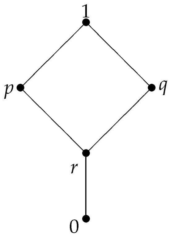
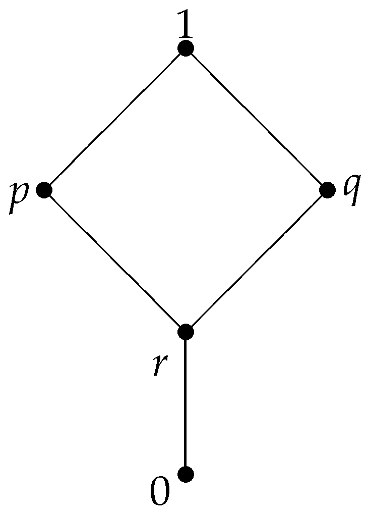
Let lattice Ω be given by Figure 1, and let $G=\{a,b,c,d\}$ be a set. Let us consider two lattice-valued equivalence relations given by Table 1 and Table 2.

Figure 1. Lattice $\Omega$ from Example 1.

Table 1. Lattice-valued equivalence relation R.

R	a	b	c	d
a	1	p	r	r
b	p	1	r	r
c	r	r	1	q
d	r	r	q	1

Table 2. Lattice-valued equivalence relation S.

S	a	b	c	d
a	1	q	p	r
b	q	1	r	r
c	p	r	1	r
d	r	r	r	1

Now, let us assume that an aggregation operator is applied to those two lattice-valued equivalence relations and that another lattice-valued equivalence relation is obtained as the result. The question is: what would be a convenient result in this case?

As expected, some of the convenient results would be a supremum or an infimum in the lattice of all $\Omega$-equivalence relations on this set $G=\{a,b,c,d\}.$ Therefore, the next two tables (Table 3 and Table 4) represent the infimum (intersection) and the supremum of these relations:

Table 3. Intersection of R and S.

$R\cap S$	a	b	c	d
a	1	r	r	r
b	r	1	r	r
c	r	r	1	r
d	r	r	r	1

Table 4. Supremum of R and S.

$R\vee S$	a	b	c	d
a	1	1	p	r
b	1	1	p	r
c	p	p	1	q
d	r	r	q	1

The intersection is computed componentwise, whereas the supremum is not. This means that the supremum can not be obtained by any aggregation operator A as $A(R,S)(x,y)=A\left(R\right(x,y),S(x,y\left)\right).$ For example, if $x=a$ and $y=d$, and A is an aggregation operator, then

$$A(R,S)(a,d)=A\left(R\right(a,d),S(a,d\left)\right)=A(r,r)$$

(5)

On the other hand, for $x=b$ and $y=c$, we have

$$A(R,S)(b,c)=A\left(R\right(b,c),S(b,c\left)\right)=A(r,r).$$

(6)

Now, the request for the result of aggregation is to be an equivalence relation. If it is the supremum, the grade of relation between a and d has to be r (see Table 4) and therefore from (5) follows $A(r,r)=r.$ At the same time, the grade of relation between b and c is p (see Table 4), and from (6) follows $A(r,r)=p$. A contradiction is obtained that supports the observation that supremum can not be a result of aggregation.

If the aggregation operator is a t-norm and the result of aggregation is the intersection (see Table 3), which is an equivalence relation.

In the following, $\Omega$-groups with the Klein group as the underlying structure are observed. Usually, since some different problems were in focus while developing $\Omega$-structures, a group is not used as the underlying structure. In that research, some groupoids were used; however, for the sake of illustration, the Klein group is now the underlying structure.

Example 2.

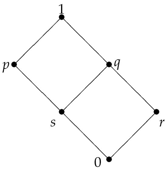
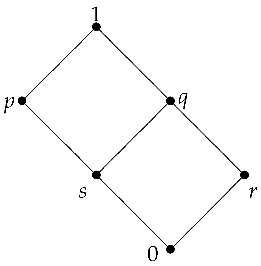
Let Ω be a lattice given by Figure 2. Let $(G,\ast {,}^{-1},e)$ be the Klein group with $G=\{e,a,b,c\},$ the binary operation given by Table 5 and the unary operation defined by $x^{-1}=x$ for all $x\in G$. Let the two Ω-groups $(G,E_1)$ and $(G,E_2)$ be defined on G by equality relations $E_1$ and $E_2$ given by Table 6 and Table 7 (respectively).

Figure 2. Lattice $\Omega$ from Example 2.

Table 5. Operation ∗.

∗	e	a	b	c
e	e	a	b	c
a	a	e	c	b
b	b	c	e	a
c	c	b	a	e

Table 6. Equality relation $E_1$.

$E_1$	e	a	b	c
e	1	r	p	0
a	r	q	0	s
b	p	0	1	r
c	0	s	r	q

Table 7. Equality relation $E_2$.

$E_2$	e	a	b	c
e	1	p	r	0
a	p	1	0	r
b	r	0	q	s
c	0	r	s	q

Now, the question is which $\Omega$-group can be a natural result of the aggregation of $E_1$ and $E_2$.

An easily deduced well-known result [17] is that the infimum $E_1\wedge E_2$ is obtained as an aggregation of $E_1$ and $E_2$ using the infimum as the aggregation operator (Table 8). Also, we can see that the supremum $E_1\vee E_2$ is not obtained as the result of an aggregation by any operator. This follows from the fact that the aggregation operator is applied componentwise. That is, if A is an arbitrary aggregation operator, then $A(E_1,E_2)(x,y)=A(E_1(x,y),E_2(x,y))$. Now, for $x=e$ and $y=c$, holds

$$A(E_1,E_2)(e,c)=A(0,0),$$

and since the grade of relation between e and c is 1 (see Table 9), the obtained conclusion is $A(0,0)=1$ which is a contradiction. Therefore, it is not possible to obtain the supremum as a result of an aggregation of $E_1$ and $E_2$.

Table 8. Infimum of $E_1$ and $E_2$.

$E_1\wedge E_2$	e	a	b	c
e	1	0	0	0
a	0	q	0	0
b	0	0	q	0
c	0	0	0	q

Table 9. Supremum of $E_1$ and $E_2$.

$E_1\vee E_2$	e	a	b	c
e	1	1	1	1
a	1	1	1	1
b	1	1	1	1
c	1	1	1	1

The next logical step is to analyze what can be the result of the aggregation of $E_1$ and $E_2$, if it is not the supremum.

The aggregation will be done by operators that are compatible with the lattice operations, i.e., as it follows from Theorem 1, by idempotent weighted lattice polynomials. It is reasonable to suppose that the result of aggregation is an $\Omega$-group from the interval

$$[E_1\wedge E_2,E_1\vee E_2].$$

Now, based on Lemma 1, functions $\mu$ should be $\Omega$-subgroups of the group G, and by detailed analyses, the conclusion is that there are five $\Omega$-valued fuzzy subgroups in the interval

$$[{\mu }_1\wedge {\mu }_2,{\mu }_1\vee {\mu }_2],$$

where ${\mu }_1\left(x\right)=E_1(x,x)$ and ${\mu }_2\left(x\right)=E_2(x,x).$ They are given by Table 10.

Table 10. $\Omega$-valued fuzzy subgroups.

$\nu$	e	a	b	c
${\nu }_1$	1	1	1	1
${\nu }_2$	1	1	q	q
${\nu }_3$	1	q	1	q
${\nu }_4$	1	q	q	1
${\nu }_5$	1	q	q	q

The next question is which one of those five options can be a result of the aggregation of the given two fuzzy subgroups, and which aggregation operator will provide such a result. Let us observe aggregation operators, knowing that they are weighted idempotent lattice polynomials. The following can be deduced:

• ${\nu }_5$ is the infimum of two lattice-valued subgroups, and this case is already discussed.
• ${\nu }_1$ is the supremum. If A is the aggregation operator, we have $A(q,q)=1$, which is a contradiction to the assumption that A is idempotent.
• ${\nu }_4$ is disregarded since $A(1,q)=q$ and $A(q,q)=1$, and A has to be monotone.
• From Table 6 and Table 7, it follows that $E_1(a,a)=q$, $E_2(a,a)=1$, $E_1(b,b)=1$ and $E_2(b,b)=q$.
• For ${\nu }_2$, $A(q,1)=1$, $A(1,q)=q$, and $A(q,q)=q$ hold.
• For ${\nu }_3$, $A(q,1)=q$, $A(1,q)=1$ and $A(q,q)=q$ hold.

Now, for A being an aggregation operator on the lattice $\Omega ,$ based on the previous discussion, the following has been deduced for the resulting relation R (Table 11).

Table 11. The resulting relation R.

R	e	a	b	c
e	1	$A(r,p)$	$A(p,r)$	0
a	$A(r,p)$	$A(q,1)$	0	$A(s,r)$
b	$A(p,r)$	0	$A(1,q)$	$A(r,s)$
c	0	$A(s,r)$	$A(r,s)$	$A(q,q)$

Since R should be transitive, we have that $R(a,e)\wedge R(e,b)\le R(a,b),$ hence $A(r,p)=0$. Similarly, it can be concluded that $A(r,s)=0.$ Finally, the conclusion is that there are at least three possibilities for the result of aggregation:

1.

the infimum,

2.

the first projection ($A(x,y)=x$), which corresponds to the case ${\nu }_2$,

3.

the second projection ($A(x,y)=y$), which corresponds to the case ${\nu }_3$.

For all cases $A(0,0)=A(r,p)=A(r,s)=0$ and $A(1,1)=1$ hold. Therefore, $A(r,0)=A(p,0)=A(s,0)=0,$ and some of the obvious options for the result of aggregation are the following:

1.

The aggregation of $E_1$ and $E_2$ is the infimum.

2.

The aggregation of $E_1$ and $E_2$ is $E_1$.

3.

The aggregation of $E_1$ and $E_2$ is $E_2$.

3.1. Aggregation of $\Omega$-Groups

The problem of aggregation of $\Omega$-groups is complex. It includes the aggregation of lattice-valued fuzzy groups, aggregation of lattice-valued equivalence relations and aggregation of relations compatible with the algebraic structure.

3.1.1. General Case of Aggregation of $\Omega$-Groups

We prove the following theorem without the condition that $\Omega$ is distributive lattice. We also do not require that the aggregation operator is compatible with the congruence relations on lattices.

Theorem 4.

Let $(\Omega ,\wedge ,\vee )$ be a complete lattice, let $n\in N$ and let $A:{\Omega }^n\to \Omega$ be an aggregation operator on lattice Ω. Then, for every algebra $\mathcal{G}=(G,\ast ,-1,e)$, the result of aggregation of Ω-groups on $\mathcal{G}$ by A is an Ω-group on $\mathcal{G}$ if and only if A dominates ∧, i.e., if for all $a_1,\dots ,a_n,b_1,\dots ,b_n\in \Omega$ the following holds:

$$A(a_1,\dots ,a_n)\wedge A(b_1,\dots ,b_n)=A(a_1\wedge b_1,\dots ,a_n\wedge b_n).$$

Proof. 

Since $A:{\Omega }^n\to \Omega$ is an aggregation operator on lattice $\Omega$, due to monotonicity, from $a_i\wedge b_i\le a_i$ and $a_i\wedge b_i\le b_i$, it follows that

$$A(a_1\wedge b_1,\dots ,a_n\wedge b_n)\le A(a_1,\dots ,a_n)\wedge A(b_1,\dots ,b_n).$$

Hence, the condition $A(a_1,\dots ,a_n)\wedge A(b_1,\dots ,b_n)=A(a_1\wedge b_1,\dots ,a_n\wedge b_n)$ is equivalent to $A(a_1\wedge b_1,\dots ,a_n\wedge b_n)\le A(a_1,\dots ,a_n)\wedge A(b_1,\dots ,b_n)$ (the domination of A over ∧).

Suppose that A dominates $\wedge .$ Let $\mathcal{G}=(G,\ast ,-1,e)$ be an algebra and let $(\mathcal{G},E_1)$, …, $(\mathcal{G},E_n)$ be a family of $\Omega$-groups. Let E be a relation obtained by aggregation of $E_1$, …, $E_n$ based on A:

$$E(x,y)=A(E_1,\dots ,E_n)(x,y)=A(E_1(x,y),\dots ,E_n(x,y)).$$

It should be shown that E is symmetric, transitive and compatible with operations ∗, ⁻¹ and that $E(e,e)=1$. Moreover, we need to prove that the identities (1), (2) and (3) (identities for $\Omega$-groups) are fulfilled.

• It is easy to see that symmetry and transitivity of E follow in a manner similar to the classical results in [18] for $min$-transitivity. Indeed, for transitivity,

  $$E(x,y)\wedge E(y,z)=A(E_1(x,y),\dots ,E_n(x,y))\wedge A(E_1(y,z),\dots ,E_n(y,z))\le$$

  $$\le A(E_1(x,y)\wedge E_1(y,z),\dots ,E_n(x,y)\wedge E_n(y,z))\le$$

  $$\le A(E_1(x,z),\dots ,E_n(x,z))=A(E_1,\dots ,E_n)(x,z).$$
• Compatibility with ∗ is proved in the sequel.

  $$E(x,y)\wedge E(z,t)=A(E_1(x,y),\dots ,E_n(x,y))\wedge A(E_1(z,t),\dots ,E_n(z,t))\le$$

  $$\le A(E_1(x,y)\wedge E_1(z,t),\dots ,E_n(x,y)\wedge E_n(z,t))\le$$

  $$\le A(E_1(x\ast z,y\ast t),\dots ,E_n(x\ast z,y\ast t))=A(E_1,\dots ,E_n)(x\ast z,y\ast t),$$

  where the last part is based on the compatibility of $E_1$,…, $E_n$ and the monotonicity of A.
• Similarly, we prove compatibility with ⁻¹ and that $E(e,e)=1.$
• The next step is to show that (1) (associativity) is fulfilled. Let $\mu \left(x\right)=E(x,x).$ Now, the following holds

  $$\mu \left(x\right)\wedge \mu \left(y\right)\wedge \mu \left(y\right)=E(x,x)\wedge E(y,y)\wedge E(z,z)=$$

  $$A(E_1(x,x),\dots ,E_n(x,x))\wedge A(E_1(y,y),\dots ,E_n(y,y))\wedge A(E_1(z,z),\dots ,E_n(z,z))\le$$

  $$\le A(E_1(x,x)\wedge E_1(y,y)\wedge E_1(z,z),\dots ,E_n(x,x)\wedge E_n(y,y)\wedge E_n(z,z))\le$$

  $$\le A(E_1((x\ast y)\ast z,x\ast (y\ast z)),\dots ,E_n((x\ast y)\ast z,x\ast (y\ast z)))=$$

  $$=A(E_1,\dots ,E_n)((x\ast y)\ast z,x\ast (y\ast z))=E((x\ast y)\ast z,x\ast (y\ast z)),$$

  where the last part is based on the fact that the associativity is satisfied in $\Omega$-groups $(\mathcal{G},E_1)$, …, $(\mathcal{G},E_n)$, and on the monotonicity of A.
• Identities (2) and (3) for E are proved analogously.

To prove the converse, suppose that A aggregates $\Omega$-groups. This means that the result of aggregating the lattice-valued equality relations that satisfy the group identities by A is a lattice-valued equality relation that satisfies the group identities. Consequently, for every family of $\Omega$-groups, the aggregation is also an $\Omega$-group, and we utilize this fact in the sequel.

We have to prove that $A(x_1,\dots ,x_n)\wedge A(y_1,\dots ,y_n)=A(x_1\wedge y_1,\dots ,x_n\wedge y_n)$ for all $x_1,\dots ,x_n,y_1,\dots ,y_n\in \Omega$.

Look at the pair of elements $x_i$, $y_i\in \Omega$.

There are three possibilities:

1.

$x_i=y_i$.

2.

$x_i\ne y_i$ and elements are comparable: $x_i\le y_i$. Then, $x_i\wedge y_i=x_i$. The case $y_i\le x_i$ is analogous.

3.

Elements are incomparable, which means that $x_i,y_1$ and $x_i\wedge y_i$ are three different elements.

Now, we take a convenient family of n $\Omega$-groups and the aggregation of this family should be an $\Omega$-group. We will use this fact in the sequel.

We will construct $\Omega$ groups from a crisp group using Theorem 1. If $\mathcal{G}=(G,\ast {,}^{-1},e)$ is a group then $(\mathcal{G},E)$ is an $\Omega$-group if and only if all the cuts $E_p$, $p\in \Omega$ are weak congruences on $\mathcal{G}$.

Let G be a 6-element cyclic group $G=\{e,a,b,c,$$d,f\}$ with $a^6=e$, $a^2=b$, $a^3=c,$ $a^4=d$ and $a^5=f$. This group has two subgroups, $G_1=\{e,b,d\}$ and $G_2=\{e,c\}$

Now, we look at the elements $x_i,y_i\in \Omega .$ There are three possibilities as noted above.

1.

Let $x_i=y_i$. Then, we define $\Omega$-group $E^i$ on $\{e,a,b,c,d,f\}$ as follows:

$E^i(e,e)=1$ and $E^i(y,t)=0$ if $y\ne e$ or $t\ne e.$

Here, we have only two (different) cuts, $E_1^i=\left\{(e,e)\right\}$ and $E_0^i=G^2.$ Since they are squares of subalgebras, they are also weak congruences of $\mathcal{G}$.

2.

Let $x_i\ne y_i$ and let $x_i\le y_i$. Then, we define $\Omega$-group $E^i$ on $\{e,a,b,c,d,f\}$ as follows:

$E^i(e,e)=1,$ $E^i(c,e)=E^i(e,c)=E^i(c,c)=y_i$, $E^i(z,t)=x_i$, for all $z,t$ which are not both in $\{e,c\}.$

Here, cuts are $E_1^i=\left\{(e,e)\right\},$ $E_{y_i}^i=G_2^2$ (square of subgroup $G_2$), and $E_{x_i}^i=G^2.$ All other cuts are equal to some of these three squares of subgroups and they are weak congruences. Hence, $(\mathcal{G},E^i)$ is an $\Omega$-group.

3.

Finally, let $x_i$ and $y_i$ be incomparable. Then, $x_i,y_i,x_i\wedge y_i$ are different elements of $\Omega$. Now, we define $E^i$ with:

$E^i(e,e)=1$, $E^i(e,b)=E^i(e,d)=E^i(b,d)=E^i(d,d)=E^i(d,b)=E^i(b,b)=E^i(b,e)=E^i(d,e)=x_i$, $E^i(c,c)=E^i(e,c)=E^i(c,e)=y_i$. Let $E^i(z,t)=x_i\wedge y_i$ otherwise. In particular, we have that $E^i(b,c)=x_i\wedge y_i$.

The cuts here are $E_1^i=\left\{(e,e)\right\},$ $E_{x_i}^i=G_1^2,$ $E_{y_i}^i=G_2^2$ and $E_{x_i\wedge y_i}^i=G^2.$ All other cuts are the same as one of these and since the cuts are weak congruences, $(\mathcal{G},E^i)$ is also an $\Omega$-group.

So, we have (in all three cases) $E^i(e,b)=x_i$, $E^i(e,c)=y_i$ and $E^i(b,c)=x_i\wedge y_i.$

Now, for every $x_i$, $y_i\in \Omega$, we take an equality relation $E^i$ on $\mathcal{G}=(G,\ast {,}^{-1},e)$, such that $(\mathcal{G},E_i)$ is an $\Omega$-group, as described above.

Now, the aggregation of all $\Omega$-groups $(\mathcal{G},E^i)$, for $i\in \{1,2,\dots ,n\}$ is an $\Omega$-group.

Hence, $A(E^1,\dots ,E^n)$ should also be transitive.

$$A(E^1,\dots ,E^n)(b,e)\wedge A(E^1,\dots ,E^n)(e,c)\le A(E^1,\dots ,E^n)(b,c),$$

Hence,

$$A(x_1,\dots ,x_n)\wedge A(y_1,\dots ,y_n)=$$

$$A(E^1(b,e),\dots ,E^n(b,e))\wedge A(E^1(e,c),\dots ,E^n(e,c))=$$

$$A(E^1,\dots ,E^n)(b,e)\wedge A(E^1,\dots ,E^n)(e,c)\le A(E^1,\dots ,E^n)(b,c)=$$

$$A(E^1(b,c),\dots ,E^n(b,c))=A(x_1\wedge y_1,\dots ,x_n\wedge y_n).$$

□

3.1.2. Case of Binary Aggregation of $\Omega$-Groups for Distributive Lattice $\Omega$

In this section, Theorem 4, with the help of Theorems 2 and 3, will be considered for the special case of a complete distributive lattice.

In what follows, some facts about a weighted lattice polynomial function combining Theorems 2 and 3 are stated in the following four claims.

Claim 1.

If A is idempotent, and $A_j$ from Theorem 3 is the empty set, then the related coefficient $a_j=0\in \Omega$. This follows from the fact that $A(0,\dots ,0)=0.$

Claim 2.

If A is idempotent, then ${\bigvee }_{i=1}^k{a}_i=1$. This follows from the fact $A(1,\dots ,1)=1.$

Claim 3.

If ${\bigvee }_{i=1}^k{a}_i=1$, then A is idempotent.

Claim 4.

In the formula from Theorem 3, we can consider that all summands are present with allowing that some of the coefficients are $0\in \Omega$.

Hence, by Claim 1, the idempotent weighted lattice function on lattice $\Omega$, which is at the same time an aggregation operator with two variables, is given by:

$$A(x_1,x_2)=(a\wedge x_1)\vee (b\wedge x_2)\vee (c\wedge x_1\wedge x_2),fora,b,c\in \Omega , a\vee b\vee c=1.$$

Now, the following theorem can be proved.

Theorem 5.

Let Ω be a complete distributive lattice and let $A:{\Omega }^2\to \Omega$ be an aggregation operator of the form

$$A(x_1,x_2)=(a\wedge x_1)\vee (b\wedge x_2)\vee (c\wedge x_1\wedge x_2).$$

Then, $A(x_1,x_2)\wedge A(y_1,y_2)=A(x_1\wedge y_1,x_2\wedge y_2)$ if and only if $a\wedge b=0$.

Proof. 

Let us suppose that $A(x_1,x_2)\wedge A(y_1,y_2)=A(x_1\wedge y_1,x_2\wedge y_2),$ therefore

$$((a\wedge x_1)\vee (b\wedge x_2)\vee (c\wedge x_1\wedge x_2))\wedge ((a\wedge y_1)\vee (b\wedge y_2)\vee (c\wedge y_1\wedge y_2))=$$

$$=(a\wedge x_1\wedge y_1)\vee (a\wedge b\wedge x_1\wedge y_2)\vee (a\wedge c\wedge x_1\wedge y_1\wedge y_2)\vee (a\wedge b\wedge x_2\wedge y_1)\vee (b\wedge x_2\wedge y_2)$$

$$\vee (b\wedge x_2\wedge c\wedge y_1\wedge y_2)\vee (a\wedge y_1\wedge c\wedge x_1\wedge x_2))\vee (b\wedge y_2\wedge c\wedge x_1\wedge x_2)\vee (c\wedge x_1\wedge x_2\wedge y_1\wedge y_2).$$

Now, the property of absorption insures:

$$(a\wedge x_1\wedge y_1)\vee (a\wedge c\wedge x_1\wedge y_1\wedge y_2)=a\wedge x_1\wedge y_1,$$

$$(b\wedge x_2\wedge y_2)\vee (b\wedge x_2\wedge c\wedge y_1\wedge y_2)=b\wedge x_2\wedge y_2,$$

$$(a\wedge x_1\wedge y_1)\vee (a\wedge y_1\wedge c\wedge x_1\wedge x_2)=a\wedge x_1\wedge y_1,$$

and

$$(b\wedge x_2\wedge y_2)\vee (b\wedge y_2\wedge c\wedge x_1\wedge x_2)=b\wedge x_2\wedge y_2.$$

Hence,

$$((a\wedge x_1)\vee (b\wedge x_2)\vee (c\wedge x_1\wedge x_2))\wedge ((a\wedge y_1)\vee (b\wedge y_2)\vee (c\wedge y_1\wedge y_2))=$$

$$=(a\wedge x_1\wedge y_1)\vee (a\wedge b\wedge x_1\wedge y_2)\vee (a\wedge b\wedge x_2\wedge y_1)\vee (b\wedge x_2\wedge y_2)\vee (c\wedge x_1\wedge x_2\wedge y_1\wedge y_2).$$

The last formula for all $x_1,x_2,y_1,y_2\in \Omega$ should be equal to

$$(a\wedge x_1\wedge y_1)\vee (b\wedge x_2\wedge y_2)\vee (c\wedge x_1\wedge x_2\wedge y_1\wedge y_2).$$

Let $x_1=y_2=1$ and $x_2=y_1=0.$ Then, we have the following

$$(a\wedge x_1\wedge y_1)\vee (a\wedge b\wedge x_1\wedge y_2)\vee (a\wedge b\wedge x_2\wedge y_1)\vee (b\wedge x_2\wedge y_2)\vee (c\wedge x_1\wedge x_2\wedge y_1\wedge y_2)=a\wedge b$$

and

$$(a\wedge x_1\wedge y_1)\vee (b\wedge x_2\wedge y_2)\vee (c\wedge x_1\wedge x_2\wedge y_1\wedge y_2)=0.$$

Therefore, $a\wedge b=0.$

To prove the opposite, let us suppose that $a\wedge b=0.$ It should be shown that $A(x_1,x_2)\wedge A(y_1,y_2)=A(x_1\wedge y_1,x_2\wedge y_2),$ which is equivalent to

$$((a\wedge x_1)\vee (b\wedge x_2)\vee (c\wedge x_1\wedge x_2))\wedge ((a\wedge y_1)\vee (b\wedge y_2)\vee (c\wedge y_1\wedge y_2))=$$

$$=(a\wedge x_1\wedge y_1)\vee (a\wedge b\wedge x_1\wedge y_2)\vee (a\wedge b\wedge x_2\wedge y_1)\vee (b\wedge x_2\wedge y_2)\vee (c\wedge x_1\wedge x_2\wedge y_1\wedge y_2)=$$

$$=(a\wedge x_1\wedge y_1)\vee (b\wedge x_2\wedge y_2)\vee (c\wedge x_1\wedge x_2\wedge y_1\wedge y_2),$$

and this is true for $a\wedge b=0.$ □

Corollary 1.

Let Ω be a complete distributive lattice. Then $A:{\Omega }^2\to \Omega$ is a compatible aggregation operator on Ω such that for every algebra $\mathcal{G}=(G,\ast ,-1,e)$, the result of aggregation of Ω-groups on $\mathcal{G}$ by A is an Ω-group on $\mathcal{G}$ if and only if $A(x_1,x_2)=(a\wedge x_1)\vee (b\wedge x_2)\vee (c\wedge x_1\wedge x_2)$, $a\wedge b=0$ and $a\vee b\vee c=1$.

Proof. 

Let $A:{\Omega }^2\to \Omega$ be a compatible aggregation operator on $\Omega$ such that for every algebra $\mathcal{G}=(G,\ast ,-1,e)$, the result of aggregation of $\Omega$-groups on $\mathcal{G}$ by A is an $\Omega$-group on $\mathcal{G}$. Then, by the fact that $\Omega$ is a distributive lattice and that A is compatible, A is, by Theorem 2, a weighted idempotent lattice polynomial function. By Theorem 3, it is in the form $A(x_1,x_2)=(a\wedge x_1)\vee (b\wedge x_2)\vee (c\wedge x_1\wedge x_2),$ with $a\vee b\vee c=1$. By Theorem 4, $A(x_1,x_2)\wedge A(y_1,y_2)=A(x_1\wedge y_1,x_2\wedge y_2)$ and by Theorem 5, $a\wedge b=0$.

To prove the converse, suppose that $A(x_1,x_2)=(a\wedge x_1)\vee (b\wedge x_2)\vee (c\wedge x_1\wedge x_2)$, $a\wedge b=0$ and $a\vee b\vee c=1$. By Theorem 5, $A(x_1,x_2)\wedge A(y_1,y_2)=A(x_1\wedge y_1,x_2\wedge y_2)$. By Theorem 4, for every algebra $\mathcal{G}=(G,\ast ,-1,e)$, the result of aggregation of $\Omega$-groups on $\mathcal{G}$ by A is an $\Omega$-group on $\mathcal{G}$. By Claim 3, A is idempotent. Since A is a weighted idempotent lattice polynomial function, by Theorem 2, it is a compatible aggregation operator. □

Example 3.

Now, we can find more results of aggregation of Ω-groups from Example 2. Let Ω be a lattice given by Figure 2. Using Corollary 1, aggregation operators that aggregate Ω-groups, are given by:

$$A(x_1,x_2)=(a\wedge x_1)\vee (b\wedge x_2)\vee (c\wedge x_1\wedge x_2),$$

with $a\wedge b=0$ and $a\vee b\vee c=1$. We can easily find all triples of elements $a,b,c\in \Omega$ satisfying these conditions, however, now we present only two examples:

1.

$A_1(x_1,x_2)=(p\wedge x_1)\vee (r\wedge x_2)$

2.

$A_2(x_1,x_2)=(p\wedge x_1)\vee (q\wedge x_1\wedge x_2).$

The above aggregation operators generate two Ω-groups $(G,E)$ (Table 12) and $(G,F)$ (Table 13), respectively.

Table 12. Equality relation E.

E	e	a	b	c
e	1	0	1	0
a	0	q	0	q
b	1	0	1	0
c	0	q	0	q

Table 13. Equality relation F.

F	e	a	b	c
e	1	0	p	0
a	0	q	0	s
b	p	0	1	0
c	0	s	0	q

In what follows, we present a consequence of the obtained results, now applied to fuzzy groups. Namely, if $(G,E)$ is an Ω-group, then the mapping $\mu :G\to \Omega$, defined by $\mu \left(x\right)=E(x,x),$ is a lattice-valued fuzzy group, and these are structures of further interest.

Lemma 2.

Let $\mathcal{G}=(G,\ast {,}^{-1},e)$ be a group and let $\mu :G\to \Omega$ be a lattice-valued fuzzy group, where Ω is a lattice. Let a lattice-valued relation $E:G^2\to \Omega$ be defined by

$$E(x,y)=\left\{\begin{array}{cc}0\hfill & \mathrm{if}x\ne y,\hfill \\ \mu \left(x\right)\hfill & \mathrm{if}x=y.\hfill \end{array}\right.$$

Then, $(\mathcal{G},E)$ is an Ω-group.

Proof. 

By the requirement that $\mu$ is a lattice-valued group, we have that $\mu \left(x\right)\wedge \mu \left(x\right)\le \mu (x\ast y)$, $\mu \left(x\right)\le \mu \left(x^{-1}\right)$ and $\mu \left(e\right)=1.$ It is straightforward that E is symmetric and transitive. Now, we have to prove that E is compatible with the operations ∗ and ⁻¹. Let $x,y,z,t\in G$. We have to prove $E(x,y)\wedge E(z,t)\le E(x\ast z,y\ast t).$ Since the only non-trivial case is when $x=y$ and $z=t$, we have that $E(x,x)\wedge E(z,z)=\mu \left(x\right)\wedge \mu \left(z\right)\le \mu (x\ast z)=E(x\ast z,x\ast z).$

We also have that $E(x,x)=\mu \left(x\right)\le \mu \left(x^{-1}\right)=E(x^{-1},x^{-1}).$

Now, we have that E is a lattice-valued equality and by Lemma 1, $(\mathcal{G},\ast )$ is an $\Omega$-group.

□

Corollary 2.

Let Ω be a distributive lattice and let $A:{\Omega }^2\to \Omega$ be an aggregation operator given by

$$A(x_1,x_2)=(a\wedge x_1)\vee (b\wedge x_2)\vee (c\wedge x_1\wedge x_2),$$

where $a\wedge b=0$ and $a\vee b\vee c=1$. Then, the result of the aggregation of lattice-valued fuzzy groups by A is a lattice-valued fuzzy group.

3.1.3. On n-Ary Aggregation Operators

Using the techniques as in Theorem 5, it is possible to formulate a statement (a necessary and sufficient condition) for n-ary aggregation operators to dominate the infima, (and by Theorem 4 to aggregate $\Omega$-groups to $\Omega$-group). However, in this text, we provide only a special case of n-ary aggregation operator that is defined iteratively from a binary aggregation operator (from Theorem 5). As a first step, we prove that the binary aggregation operator is associative.

Lemma 3.

The aggregation operator

$$A(x_1,x_2)=(a\wedge x_1)\vee (b\wedge x_2)\vee (c\wedge x_1\wedge x_2),$$

with $a,b,c\in \Omega ,a\wedge b=0$ and $a\vee b\vee c=1$ on distributive lattice Ω is associative, i.e.,

$$A(x_1,A(x_2,x_3))=A(A(x_1,x_2),x_3).$$

Proof. 

Let A be an aggregation operator that fulfills all given requirements. Then,

$$A(x_1,A(x_2,x_3))=$$

$$=(a\wedge x_1)\vee (b\wedge ((a\wedge x_2)\vee (b\wedge x_3)\vee (c\wedge x_2\wedge x_3)))\vee (c\wedge x_1\wedge ((a\wedge x_2)\vee (b\wedge x_3)\vee (c\wedge x_2\wedge x_3)))$$

$$=(a\wedge x_1)\vee (b\wedge x_3)\vee (c\wedge x_1\wedge x_2\wedge x_3),$$

and

$$A(A(x_1,x_2),x_3)=$$

$$=(a\wedge ((a\wedge x_1)\vee (b\wedge x_2)\vee (c\wedge x_1\wedge x_2)))\vee (b\wedge x_3)\vee (c\wedge ((a\wedge x_1)\vee (b\wedge x_2)\vee (c\wedge x_1\wedge x_2))\wedge x_3)=$$

$$=(a\wedge x_1)\vee (b\wedge x_3)\vee (c\wedge x_1\wedge x_2\wedge x_3).$$

□

Theorem 6.

Let A be a binary aggregation operator: $A:{\Omega }^2\to \Omega$, defined by

$$A(x_1,x_2)=(a\wedge x_1)\vee (b\wedge x_2)\vee (c\wedge x_1\wedge x_2),$$

with $a,b,c\in \Omega ,a\wedge b=0$ and $a\vee b\vee c=1$ on complete distributive lattice Ω. Let $B_n:{\Omega }^n\to \Omega$ be an n-ary function, defined by:

$$B(x_1,\dots ,x_n)=A(A(\dots (A(x_1,x_2),x_3),\dots .,x_n)\dots .).$$

Then, B is an n-ary aggregation operator and the result of the aggregation of Ω-groups by B is an Ω-group.

Proof. 

The proof is based on induction on n.

Let $n=2$. Then, $B_2(x_1,x_2)=A(x_1,x_2)$ is an aggregation operator and the result of aggregation of $\Omega$-groups by B is a $\Omega$-group by Theorem 3.

Suppose that

$$B_{n-1}(x_1,\dots ,x_{n-1})=A(A(\dots (A(x_1,x_2),x_3),\dots .,x_{n-1})\dots .)$$

is an aggregation operator (idempotent and monotone) and that the result of aggregation of $\Omega$-groups by B is an $\Omega$-group.

Now, $B_n(x_1,\dots ,x_n)=A\left(B_{n-1}(x_1,\dots ,x_{n-1},x_n)\right),$ and from $B_{n-1}(x,\dots ,x)=x$ follows

$$B_n(x,\dots ,x)=A(x,x)=x.$$

Similarly, we prove monotonicity.

Let us suppose that $B_{n-1}$ aggregates $n-1$ $\Omega$-groups to a new $\Omega$-groups, i.e., that $(G,B_{n-1}(E_1,\dots ,E_{n-1}))$ is an $\Omega$-group obtained by aggregation of $n-1$ $\Omega$ groups $(G,E_1)$,….$(G,E_{n-1}).$

Now, let us observe n $\Omega$-groups $(G,E_1)$,….,$(G,E_{n-1}),$ $(G,E_n)$. The aggregation operator

$$B_n(E_1,\dots ,E_n)=A(B_{n-1}(E_1,\dots ,E_{n-1}),E_n))$$

generates an $\Omega$-group since A aggregates $\Omega$-groups and $(G,B_{n-1}(E_1,\dots ,E_{n-1}))$ is an $\Omega$-group. □

3.1.4. Case of Classical Fuzzy Set and Applications

Since $[0,1]$ interval is also a distributive complete lattice, all the results are also valid in the classical (fuzzy) case.

Moreover, it is also valid for some special aggregation operators, like discrete Sugeno integrals (see e.g., [12,19]). It is proved in [13] that a function $f:{[0,1]}^n\to [0,1]$ is an n-ary Sugeno integral if and only if it is an idempotent weighted linear polynomial function. Hence, Corollary 1 is valid in the case of discrete Sugeno integrals.

There are very prominent applications, especially in digital forensics. Particular emphasis is on the Sugeno integral as a qualitative aggregation operator, and its lattice-based form is a good choice for aggregating heterogeneous and ordinal forensic data [20]. The intended approach enables the fusion of multiple sources of digital data, such as files, logs, and network traces, while preserving the possible imprecision of forensic data [21]. Additionally, the aggregation of weak congruences with a Sugeno-type aggregation operator supports flexibility while working with incomplete, noisy, or manipulated evidence. Moreover, applications of lattice-valued Sugeno integrals are possible for tasks such as event correlation and timeline reconstruction with particular attention to explainability and transparency, which are essential requirements in forensic and legal settings. This line of research aims to provide an applicable connection between abstract algebraic aggregation theory, fuzzy systems, and digital forensic analysis.

As already pointed out, lattice-valued fuzzy notions generalize traditional fuzzy notions using membership degrees from a complete lattice rather than the $[0,1]$-real interval, providing enhanced modeling for complex, structured uncertainty. There are many possible applications based on aggregations of lattice-based data, especially in multi-criteria decision making (where a lattice models multi-dimensional data) and in complex preference modeling (see e.g., [22,23,24]).

4. Conclusions

In this paper, we investigated the aggregation of lattice-valued fuzzy algebraic structures, with particular emphasis on fuzzy groups and $\Omega$-groups, focusing on the preservation of algebraic properties under aggregation. The presented approach starts from the desired outcome of the aggregation process, namely the preservation of the fuzzy group structure, and subsequently analyzes which aggregation operators are capable of providing this result. We established necessary and sufficient conditions under which aggregation operators on complete lattices preserve the structure of $\Omega$-groups and lattice-valued fuzzy groups. The lattice-valued framework adopted in this work provides a general and flexible setting for studying aggregation beyond the classical real-valued case. One line of future research will be the potential of Sugeno integral on lattices as an aggregation operator for fuzzy groups and related algebraic structures. Moreover, we will focus on non-componentwise aggregations of algebraic structures (e.g., using closure constructions.)

References

- Ardanza-Trevijano, S.; Chasco, M.J.; Elorza, J.; de Natividade, M.; Talavera, F.J. Aggregation of T-subgroups. Fuzzy Sets Syst. 2023, 463, 108390. [Google Scholar] [CrossRef] [Scilit]
- Bejines, C.; Chasco, M.J.; Elorza, J. Aggregation of fuzzy subgroups. Fuzzy Sets Syst. 2021, 418, 170–184. [Google Scholar] [CrossRef] [Scilit]
- Talavera, F.J.; Ardanza-Trevijano, S.; Bragard, J.; Elorza, J. Aggregation of T-subgroups of groups whose subgroup lattice is a chain. Fuzzy Sets Syst. 2023, 473, 108717. [Google Scholar] [CrossRef] [Scilit]
- Štajner-Papuga, I.; Tepavčević, A. A Note on Aggregation of T-Fuzzy Subgroups. In Computational Intelligence and Mathematics for Tackling Complex Problems 6; Kóczy, L.T., Medina, J., Kowalski, P.A., Ramírez-Poussa, E., Eds.; Studies in Computational Intelligence; Springer: Cham, Switzerland, 2026; Volume 1222. [Google Scholar] [CrossRef] [Scilit]
- Halaš, R.; Pócs, J.; Pócsová, J. Remarks on Sugeno Integrals on Bounded Lattices. Mathematics 2022, 10, 3078. [Google Scholar] [CrossRef] [Scilit]
- Karaçal, F.; Mesiar, R. Aggregation functions on bounded lattices. Int. J. Gen. Syst. 2017, 46, 37–51. [Google Scholar] [CrossRef] [Scilit]
- Budimirović, B.; Budimirović, V.; Šešelja, B.; Tepavčević, A. E-fuzzy groups. Fuzzy Sets Syst. 2016, 289, 94–112. [Google Scholar] [CrossRef] [Scilit]
- Jimenez, J.; Serrano, M.L.; Šešelja, B.; Tepavčević, A. Omega-rings. Fuzzy Sets Syst. 2023, 455, 183–197. [Google Scholar] [CrossRef] [Scilit]
- Šešelja, B.; Tepavčević, A. Ω-group in the Language of Ω-groupiods. Fuzzy Sets Syst. 2019, 397, 152–167. [Google Scholar] [CrossRef] [Scilit]
- Sánchez, T.C.; Fuster-Parra, P.; Valero, O. The aggregation of transitive fuzzy relations revisited. Fuzzy Sets Syst. 2022, 446, 243–260. [Google Scholar] [CrossRef] [Scilit]
- Li, D.; Yao, Y. Aggregation of I-transitive fuzzy relations and fuzzy preference relations. Comp. Appl. Math. 2024, 43, 208. [Google Scholar] [CrossRef] [Scilit]
- Halaš, R.; Mesiar, R.; Pócs, J. Congruences and the discrete Sugeno integrals on bounded distributive lattices. Inf. Sci. 2016, 367–368, 443–448. [Google Scholar] [CrossRef] [Scilit]
- Marichal, J.-L. Weighted lattice polynomials. Discret. Math. 2009, 309, 814–820. [Google Scholar] [CrossRef] [Scilit]
- Šešelja, B.; Stepanović, V.; Tepavčević, A. A note on representation of lattices by weak congruences. Algebra Univers. 2012, 68, 287–291. [Google Scholar] [CrossRef] [Scilit]
- Beliakov, G.; Pradera, A.; Calvo, T. Aggregation Functions: A Guide for Practitioners; Studies in Fuzziness and Soft Computing; Springer: Berlin/Heidelberg, Germany, 2007. [Google Scholar]
- Grabisch, M.; Marichal, J.-L.; Mesiar, R.; Pap, E. Aggregation Functions; Cambridge University Press: Cambridge, UK, 2009. [Google Scholar]
- Klement, E.P.; Mesiar, R.; Pap, E. Triangular Norms, Volume 8 of Trends in Logic; Kluwer Academic Publishers: Dordrecht, The Netherlands, 2000. [Google Scholar]
- Saminger, S.; Mesiar, R.; Bodenhofer, U. Domination of aggregation operators and preservation of transitivity. Int. J. Uncertain. Fuzziness Knowl.-Based Syst. 2002, 10, 11–35. [Google Scholar] [CrossRef] [Scilit]
- Halaš, R.; Mesíar, R.; Pócs, J. A new characterization of the discrete Sugeno integral. Inf. Fusion 2016, 29, 84–86. [Google Scholar] [CrossRef] [Scilit]
- Borzová, J.; Hutník, O.; Kleinová, M. Chain-based Sugeno-like operators: A new take on the Sugeno integral as a scientometric tool. Fuzzy Sets Syst. 2025, 521, 109578. [Google Scholar] [CrossRef] [Scilit]
- Stoffel, K.; Cotofrei, P.; Han, D. Fuzzy methods for forensic data analysis. In Proceedings of the 2010 International Conference of Soft Computing and Pattern Recognition, Cergy-Pontoise, France, 7–10 December 2010; pp. 23–28. [Google Scholar] [CrossRef] [Scilit]
- El-Zekey, M.; Medina, J.; Mesiar, R. Lattice-based sums. Inf. Sci. 2013, 223, 270–284. [Google Scholar] [CrossRef] [Scilit]
- Ertugrul, U.; Karacal, F.; Mesiar, R. Modified ordinal sums of triangular norms and triangular conorms on bounded lattices. Int. J. Intell. Syst. 2015, 30, 807–817. [Google Scholar] [CrossRef] [Scilit]
- Wang, Z.; Wang, Y.; Tang, K. Some properties of l -fuzzy approximation spaces based on bounded integral residuated lattices. Inf. Sci. 2014, 278, 110–126. [Google Scholar] [CrossRef] [Scilit]
Disclaimer/Publisher’s Note: The statements, opinions and data contained in all publications are solely those of the individual author(s) and contributor(s) and not of MDPI and/or the editor(s). MDPI and/or the editor(s) disclaim responsibility for any injury to people or property resulting from any ideas, methods, instructions or products referred to in the content. |
© 2026 by the authors. Licensee MDPI, Basel, Switzerland. This article is an open access article distributed under the terms and conditions of the Creative Commons Attribution (CC BY) license.