Regime-Switching Fischer–Margrabe Options Pricing with Liquidity Risk and Stochastic Volatility

Abstract

This article presents a model for pricing an exchange option considering stochastic volatility and liquidity risk. The impact of liquidity risk on an asset price is considered by utilizing a liquidity discount process that is influenced by both market and asset-specific liquidity. Girsanov’s theorem is applied to transform from the real-world probability measure to equivalent probability measures, such as the risk-neutral probability measure. The Feynman–Kac theorem is applied to transform the exchange option pricing formula into the vanilla option pricing formula. The analytical expression is derived through the characteristic function approach. The accuracy of the proposed formula is validated through comparisons with Monte Carlo simulation, where the relative error remains below $0.93\%$ across different values of $S\left(0\right)$ and $\tau$. Furthermore, numerical experiments highlight that incorporating liquidity risk leads to higher option prices. As the maturity increases from $0.1$ to $2.0$, the percentage gap between the option prices increases from $1.65\%$ to $20.2\%$. Finally, sensitivity analysis is conducted to examine the influence of various parameters and to demonstrate the impact of stochastic volatility and liquidity in exchange option valuation.

1. Introduction

An exchange option is a financial derivative that grants the holder the right, but not the obligation, to exchange the value of one asset for the value of another asset at a fixed maturity date. This type of option was introduced independently by Fischer (1978) [1] and Margrabe (1978) [2]. Exchange options allow investors to hedge against unfavorable movements in the relative performance of two assets.

In Fischer’s framework, the strike price of a European option is modeled as a stochastic process, whereas Margrabe considered an option that allows the exchange of one risky asset for another at maturity. An exchange option can be viewed as a special case of a spread option, where the payoff depends on the difference between the prices of two assets, with a zero strike price. Under the assumptions of the Black–Scholes model, both Fischer and Margrabe derived closed-form pricing formulas for exchange options.

Empirical evidence has suggested that the Black–Scholes assumption of log-normally distributed asset prices fails to capture several stylised facts of asset returns, including heavy tails, volatility clustering and implied volatility smiles and skews (Fama (1965) [3]; Cont (2001) [4]). These features play a crucial role in asset pricing and risk management. As a result, numerous extensions of the Black–Scholes framework have been proposed. The stochastic volatility model is one such extension that provides a more realistic description of financial markets by allowing volatility to be a stochastic process. In these models, volatility can be correlated with the underlying asset price, a correlation that is generally negative.

Given the importance of stochastic volatility in asset price modelling, several models have been proposed to relax the unrealistic assumptions of the Black–Scholes model. Examples of stochastic volatility models studied in the literature include Hull and White (1987) [5], Stein and Stein (1991) [6] and Heston (1993) [7], which allow volatility to evolve dynamically over time.

Market liquidity refers to the ability to trade a financial asset quickly and in large quantities without significantly affecting its price. In highly liquid markets, transactions can be executed efficiently at relatively stable prices. In contrast, assets that are difficult to trade tend to command lower prices as investors require compensation for bearing liquidity risk. Empirical studies indicate that liquidity risk fluctuates over time and impacts both individual stocks and the overall market. For a detailed discussion of liquidity risk and its time-varying nature, we refer the reader to Acharya (2005) [8].

The literature examining the role of liquidity risk in asset and option pricing includes Liu and Yong (2005) [9], who modelled liquidity risk by allowing trading activity to impact asset prices and studied the replication of European contingent claims. Cetin et al. (2004) [10] introduced liquidity risk through a supply curve that depends on order size, while Madan and Cherny (2010) [11] proposed a stress-parameter-based liquidity model. Brunetti and Caldarera (2006) [12] incorporated liquidity effects via a liquidity discount factor depending on both market-wide and asset-specific liquidity. Feng et al. (2014) [13] modeled market liquidity as a stochastic process and derived pricing formulas for European options. The present article adopts the model established by Feng et al. (2014) [13] for liquidity risk.

Numerous studies have investigated exchange option pricing, and a brief literature review of exchange option pricing is presented below. Antonelli et al. (2010) [14] derived a power series expansion for the no-arbitrage price with respect to the correlation between the underlying asset and its volatility. Kim and Park (2017) [15] developed an exchange option pricing formula under stochastic volatility using multiscale asymptotic analysis. Cheang and Graces (2020) [16] incorporated jump components and stochastic volatility into the Black–Scholes framework to better capture market dynamics. Pasricha and Goel (2022) [17] obtained a closed-form solution for exchange option pricing under stochastic volatility through the iterative application of the Feynman–Kac formula.

The characteristic function-based approach is used in this article, which plays a central role in option pricing. Carr and Madan (1999) [18] introduced an efficient Fourier transform (FFT)-based approach for option valuation, which assumes an analytical characteristic function is known and derives a simple analytic expression for the Fourier transform of the option price. Fang and Oosterlee (2009) [19] proposed the Fourier–cosine (COS) method, which represents probability density functions through cosine series expansions, leading to an accurate and computationally efficient numerical evaluation of European option prices under the risk-neutral measure.

Regime-switching models provide a framework for modelling structural changes in economic conditions and financial markets. Hamilton (1989) [20] introduced discrete-time Markov regime-switching autoregressive models, which have since been widely used to model asymmetry, heavy-tailed returns, time-varying volatility, volatility clustering and nonlinear dynamics in financial time series. In these models, market conditions evolve across a finite number of regimes governed by a Markov chain.

In real financial markets, volatility not only switches between discrete regimes but also evolves continuously over time. Regime-switching stochastic volatility models therefore provide a natural generalization of regime-switching constant volatility models by combining both discrete structural changes and continuous volatility dynamics. Recent studies have incorporated regime-switching and stochastic volatility into option pricing models. Goutte et al. (2017) [21] developed a regime-switching stochastic volatility model for VIX options, assuming a perfectly liquid underlying market. He and Lin (2023) [22] extended the regime-switching framework to exchange option pricing by incorporating market liquidity risk. Subsequently, He and Lin (2024) [23] proposed a stochastic volatility model with liquidity risk for European option pricing.

Existing exchange option pricing models typically assume constant volatility and perfect liquidity, or incorporate regime switching without stochastic volatility. More recent approaches introduce liquidity risk or stochastic volatility separately; however, models that jointly incorporate regime-switching stochastic volatility, stochastic liquidity risk, and regime-dependent interest rates remain limited. The framework proposed in this paper addresses this gap by integrating these features within a unified and analytically tractable exchange option pricing model The main contributions of this paper are summarized as follows:

• The exchange option model of He and Lin (2023) [22] is extended by introducing Heston-type stochastic volatility dynamics and regime-dependent interest rates.
• The stochastic volatility–liquidity framework of He and Lin (2024) [23] is extended from European vanilla options to exchange options under regime switching.
• A semi-closed-form pricing formula is derived based on characteristic functions using an iterative Feynman–Kac approach.
• Numerical comparisons are provided to demonstrate the pricing impact of regime switching and liquidity risk relative to benchmark models.

Our results indicate that incorporating regime-switching stochastic volatility leads to higher option prices and that accounting for liquidity risk further increases option values relative to those of models with constant volatility and perfectly liquid markets.

The remainder of the paper is organized as follows. Section 2 presents the asset price dynamics under the real-world probability measure. Section 3 introduces the equivalent risk-neutral measure and derives the analytical pricing formula for the exchange option. Section 4 provides numerical validation and sensitivity analysis. Section 5 concludes the paper.

2. Model Description

Let $(\Omega ,\mathcal{F},\mathcal{P})$ be a probability space in which $\mathcal{P}$ represents the real-world probability measure. Consider a finite and fixed time horizon T. Assume that there are two types of financial assets in the market and that both are risky. These assets have imperfect liquidity, which occurs when there is an excess or lack of assets in the market. Let $X:=\left\{X\right(t\left)\right|t\in [0,T]\}$ be a continuous-time, finite-state Markov chain with the state space $\{s_1,s_2,\dots ,s_n\}$. These states can be considered different states of the economy. Let $\{{\mathcal{F}}_t^X,t\in [0,T]\}$ be the right continuous, natural filtration generated by $X.$ Without loss of generality, the state space of X can be identified with states of unit vectors $\{e_1,e_2,\dots ,e_n\}$ where $e_i\in {\mathbb{R}}^n$. Let $\Gamma =\left[{\gamma }_{ij}\right]$ is the transition rate matrix of X under $\mathcal{P}$, where ${\gamma }_{ij}$ is the transitional intensity of the chain from regime i to regime j. Then, from Elliott et al. (2005) [24],

$$dX\left(t\right)=\Gamma X\left(t\right)dt+dM\left(t\right),$$

(1)

where $\left\{M\right(t\left)\right|t\in [0,T]\}$ is a martingale process. Let ${\tilde{S}}_i\left(t\right)$ be the price of the asset i at time t when the market is perfectly liquid. The dynamics of ${\tilde{S}}_i\left(t\right)$ is given by

$${\displaystyle \frac{d{\tilde{S}}_i\left(t\right)}{{\tilde{S}}_i\left(t\right)}}={\mu }_i\left(t\right)dt+{\sigma }_i\left(t\right)d{\tilde{W}}_i\left(t\right)+\sqrt{{\nu }_i\left(t\right)}d{\tilde{B}}_i\left(t\right).$$

The short-term volatility ${\nu }_i\left(t\right)$ follows the Heston model and is given by

$$d{\nu }_i\left(t\right)={\tilde{\kappa }}_i({\tilde{\theta }}_i\left(t\right)-{\nu }_i\left(t\right))dt+{\xi }_i\sqrt{{\nu }_i\left(t\right)}d{\tilde{B}}_{i,\nu }\left(t\right)$$

where $i=1,2.$$\{{\tilde{W}}_i\left(t\right),t\in [0,T]\}$, $\{{\tilde{B}}_i\left(t\right),t\in [0,T]\}$ and $\{{\tilde{B}}_{i,\nu }\left(t\right),$$t\in [0,T]\}$ are standard Wiener processes with the correlation structure $d{\tilde{B}}_i\left(t\right)$$d{\tilde{B}}_{i,\nu }\left(t\right)={\rho }_{i}dt$ and $d{\tilde{W}}_1\left(t\right)$$d{\tilde{W}}_2\left(t\right)=\rho dt$. All other processes are assumed to be independent of each other. The expected return and long-term volatility of the $ith$ asset are ${\mu }_i\left(t\right)$ and ${\sigma }_i\left(t\right)$, respectively. The risk-free rate is represented by $r\left(t\right)$. Let $⟨·,·⟩$ be the standard inner product on ${\mathbb{R}}^n$. For $\widehat{{\mu }_1}=({\mu }_{11},{\mu }_{12},\dots ,{\mu }_{1n})$, $\widehat{{\mu }_2}=({\mu }_{21},{\mu }_{22},\dots ,{\mu }_{2n})$, $\widehat{{\sigma }_1}=({\sigma }_{11},{\sigma }_{12},\dots ,{\sigma }_{1n})$, $\widehat{{\sigma }_2}=({\sigma }_{21},{\sigma }_{22},\dots ,{\sigma }_{2n})$, $\widehat{{\theta }_1}=({\theta }_{11},{\theta }_{12},\dots ,{\theta }_{1n})$, $\widehat{{\theta }_2}=({\theta }_{21},{\theta }_{22},\dots ,{\theta }_{2n})$ and $\widehat{r}=(r_1,r_2,\dots ,r_n)$ Then,

$${\mu }_i\left(t\right)=⟨\widehat{{\mu }_i},X\left(t\right)⟩,{\sigma }_i\left(t\right)=⟨\widehat{{\sigma }_i},X\left(t\right)⟩,{\theta }_i\left(t\right)=⟨\widehat{{\theta }_i},X\left(t\right)⟩\mathrm{and}r\left(t\right)=⟨\hat{r},X\left(t\right)⟩.$$

The long-term volatility of an asset’s price process depends on economic conditions and corporate performance. Whereas short-term volatility is influenced by the trading actions of investors, here, $\kappa$ and $\xi$ are the rate of mean reversion and the volatility of volatility, and they are assumed to be constant.

The impact of liquidity on asset price is considered by discounting the asset price with a discounting process $D_i\left(t\right)$. The liquidity discount process $D_i\left(t\right)$ (for the $ith$ asset) demonstrates the impact of liquidity on the asset price, which is a function of market liquidity $\alpha \left(t\right)$ and asset-specific liquidity ${\beta }_i$. Following Feng et al. (2014) [13], it is assumed that the discount factor follows the following stochastic differential equation (SDE):

$${\displaystyle \frac{d{D}_i\left(t\right)}{D_i\left(t\right)}}=\left(-{\beta }_i\alpha \left(t\right)+{\displaystyle \frac{1}{2}}{\beta }_i^2{\left(\alpha \left(t\right)\right)}^2\right)dt-{\beta }_i\alpha \left(t\right)d{\tilde{W}}_{i,d}\left(t\right),$$

where $\alpha \left(t\right)$ is given by the following mean reverting process

$$d\alpha \left(t\right)=\tilde{a}\left(\tilde{b}-\alpha \left(t\right)\right)dt+\eta d{\tilde{W}}_{\alpha }\left(t\right),$$

with $d{\tilde{W}}_{i,d}\left(t\right)d{\tilde{W}}_{\alpha }\left(t\right)={\tilde{\rho }}_{i}dt$. The price of the assets in the market with liquidity risk is given by [12]

$$S_i\left(t\right)={\left(D_i\left(t\right)\right)}^{-1}{\tilde{S}}_i\left(t\right).$$

(2)

Given

$$\begin{array}{cc}\hfill d{\tilde{S}}_i\left(t\right)& ={\tilde{S}}_i\left(t\right)\left[{\mu }_i\left(t\right)dt+{\sigma }_i\left(t\right)d{\tilde{W}}_i\left(t\right)+\sqrt{{\nu }_i\left(t\right)}d{\tilde{B}}_i\left(t\right)\right],\hfill \\ \hfill d{D}_i\left(t\right)& =D_i\left(t\right)\left[\left({\beta }_i\alpha \left(t\right)+\frac{1}{2}{\beta }_i^2\alpha {\left(t\right)}^2\right)dt-{\beta }_i\alpha \left(t\right)d{\tilde{W}}_{i,d}\left(t\right)\right].\hfill \end{array}$$

Applying the Itô-Doeblin formula for an Itô process to $D_i{\left(t\right)}^{-1}$ then

$$d\left(D_i{\left(t\right)}^{-1}\right)=-D_i{\left(t\right)}^{-2}d{D}_i\left(t\right)+D_i{\left(t\right)}^{-3},d[D_i,D_i]\left(t\right).$$

Since

$$d[D_i,D_i]\left(t\right)={\beta }_i^2\alpha {\left(t\right)}^2{D}_i{\left(t\right)}^{2}dt,$$

we obtain

$$d\left(D_i{\left(t\right)}^{-1}\right)=D_i{\left(t\right)}^{-1}\left[\left({\beta }_i\alpha \left(t\right)+\frac{1}{2}{\beta }_i^2\alpha {\left(t\right)}^2\right)dt+{\beta }_i\alpha \left(t\right)d{\tilde{W}}_{i,d}\left(t\right)\right].$$

According to Itô’s formula,

$$d{S}_i\left(t\right)=D_i{\left(t\right)}^{-1}d{\tilde{S}}_i\left(t\right)+{\tilde{S}}_i\left(t\right)d\left(D_i{\left(t\right)}^{-1}\right)+d\left[{\tilde{S}}_i,D_i\right]\left(t\right).$$

Hence, the SDE of the liquidity-adjusted asset price process $S_i\left(t\right)$ is given by

$${\displaystyle \frac{d{S}_i\left(t\right)}{S_i\left(t\right)}}=\left({\mu }_i\left(t\right)+{\beta }_i\alpha \left(t\right)+{\displaystyle \frac{1}{2}}{\beta }_i^2{\left(\alpha \left(t\right)\right)}^2\right)dt+{\sigma }_{i,t}d{\tilde{W}}_i\left(t\right)+{\beta }_i\alpha \left(t\right)d{\tilde{W}}_{i,d}\left(t\right)+\sqrt{{\nu }_i\left(t\right)}d{\tilde{B}}_i\left(t\right).$$

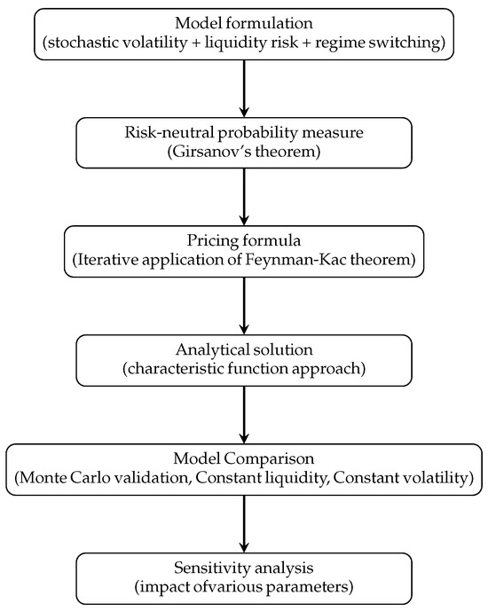
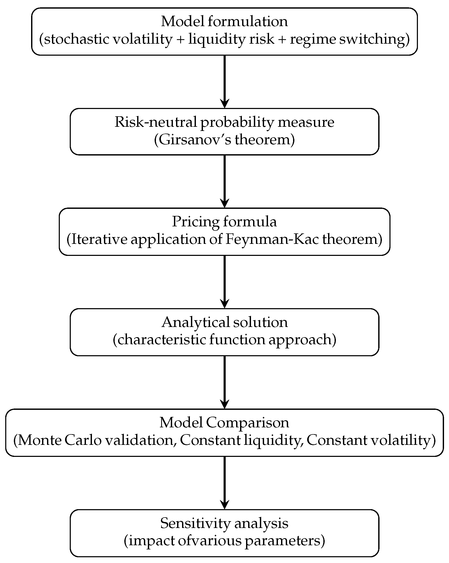
For $t\in [0,T]$, define $\{{\mathcal{F}}_t^Z$ = $\sigma \{{\tilde{W}}_{1,d}\left(u\right),{\tilde{W}}_{2,d}\left(u\right)$${\tilde{W}}_{\alpha }\left(u\right)$${\tilde{W}}_1\left(u\right)$, ${\tilde{W}}_2\left(u\right)$, ${\tilde{B}}_1\left(u\right)$, ${\tilde{B}}_2\left(u\right)$${\tilde{B}}_{1,\nu }\left(u\right) ,$${\tilde{B}}_{2,\nu }\left(u\right):$$u\le t\}$. Define a filtration $\left\{{\mathcal{F}}_t\right|t\in [0,T]\}$ where ${\mathcal{F}}_t={\mathcal{F}}_t^X\bigvee {\mathcal{F}}_t^Z$, the minimal sigma field generated by ${\mathcal{F}}_t^X$ and ${\mathcal{F}}_t^Z$. The price of the assets in an imperfectly liquid market is decided by the market-clearing condition as defined in Feng et al. (2014) [13]. Feng et al. (2016) [25] provide empirical evidence that the pricing errors of the liquidity-adjusted pricing model are fewer compared to those in the model without the liquidity risk pricing model. The flowchart of the research methodology is presented in Figure 1.

Figure 1. Flowchart of the proposed research methodology.

3. Exchange Option Price

The pricing formula for the European exchange option is presented in this section when volatility is a stochastic process and the market is affected by liquidity risk. To obtain the closed-form solution, for the exchange option with stochastic volatility and stochastic liquidity, it is essential to construct a risk-neutral measure.

3.1. Risk-Neutral Probability Measure

The market is incomplete under the described model assumptions. Hence, several equivalent martingale measures will exist. A new probability measure $\mathcal{Q}$ is defined by using Esscher transform (Elliott et al. (2005) [24]).

$$\begin{array}{cc}\hfill {\displaystyle \frac{d\mathcal{Q}}{d\mathcal{P}}}=& \exp \{-{\int }_0^t{\lambda }_1\left(s\right)d{\tilde{W}}_1\left(s\right)ds-{\int }_0^t{\lambda }_2\left(s\right)d{\tilde{W}}_2\left(s\right)-{\displaystyle \frac{1}{2}}{\int }_0^t{\lambda }_1^2\left(s\right)ds-{\displaystyle \frac{1}{2}}{\int }_0^t{\lambda }_2^2\left(s\right)ds\hfill \\ & -{\displaystyle \frac{1}{2}}{\int }_0^t{k}_1^2{\nu }_1\left(s\right)ds-{\int }_0^t{c}_1{\beta }_1\alpha \left(s\right)d{\tilde{W}}_{1,d}\left(s\right)-{\int }_0^t{c}_2{\beta }_2\alpha \left(s\right)d{\tilde{W}}_{2,d}\left(s\right)\hfill \\ & -{\int }_0^t{k}_1\sqrt{{\nu }_1\left(s\right)}d{\tilde{B}}_1\left(s\right)-{\int }_0^t{k}_2\sqrt{{\nu }_2\left(s\right)}d{\tilde{B}}_2\left(s\right)-{\displaystyle \frac{1}{2}}{\int }_0^t{c}_1^2{\beta }_1^2{\alpha }^2\left(s\right)ds\hfill \\ & -{\displaystyle \frac{1}{2}}{\int }_0^t{c}_2^2{\beta }_2^2{\alpha }^2\left(s\right)ds-{\displaystyle \frac{1}{2}}{\int }_0^t{k}_2^2{\nu }_2\left(s\right)ds-{\displaystyle \frac{1}{2}}{\int }_0^t\rho {\lambda }_1\left(s\right){\lambda }_2\left(s\right)ds\},\hfill \end{array}$$

where ${\lambda }_1\left(s\right)$ and ${\lambda }_2\left(s\right)$, $0\le s\le T$ are adapted processes. To ensure the existence of an equivalent martingale measure, the following is assumed (see Mittal and Selvamuthu (2025) [26]):

$$\begin{array}{cc}\hfill r\left(t\right)=-{\sigma }_1\left(t\right){\lambda }_1\left(t\right)-{\sigma }_1\left(t\right)\rho {\lambda }_2\left(t\right)-c_1{\beta }_1^2{\left(\alpha \left(t\right)\right)}^2& - k_1{\xi }_1{\nu }_1\left(t\right)+{\mu }_1\left(t\right)+{\beta }_1\alpha \left(t\right)+{\displaystyle \frac{1}{2}}{\beta }_1^2{\left(\alpha \left(t\right)\right)}^2,\hfill \\ \hfill r\left(t\right)=-{\sigma }_2\left(t\right){\lambda }_2\left(t\right)-{\sigma }_2\left(t\right)\rho {\lambda }_1\left(t\right)-c_2{\beta }_2^2{\left(\alpha \left(t\right)\right)}^2& - k_2{\xi }_2{\nu }_2\left(t\right)+{\mu }_2\left(t\right)+{\beta }_2\alpha \left(t\right)+{\displaystyle \frac{1}{2}}{\beta }_2^2{\left(\alpha \left(t\right)\right)}^2.\hfill \end{array}$$

If both of the above conditions are satisfied, then the discounted asset price processes, $\left\{e^{-{\int }_0^{t}r\left(s\right)ds}{S}_1\left(t\right)\right|t\in [0,T]\}$ and $\left\{e^{-{\int }_0^{t}r\left(s\right)ds}{S}_2\left(t\right)\right|t\in [0,T]\}$, are martingales under $\mathcal{Q}$. Hence, $\mathcal{Q}$ is a risk-neutral probability measure. Applying Girsanov’s theorem gives the following transformation:

$$\begin{array}{c}\hfill d{W}_1\left(t\right)=d{\tilde{W}}_1\left(t\right)+{\lambda }_1\left(t\right)dt+\rho {\lambda }_2\left(t\right)dt,d{B}_1\left(t\right)=d{\tilde{B}}_1\left(t\right)+k_1\sqrt{{\nu }_1\left(s\right)}dt,\\ \hfill d{W}_2\left(t\right)=d{\tilde{W}}_2\left(t\right)+{\lambda }_2\left(t\right)dt+\rho {\lambda }_1\left(t\right)dt,d{B}_2\left(t\right)=d{\tilde{B}}_2\left(t\right)+k_2\sqrt{{\nu }_2\left(s\right)}dt,\\ \hfill d{B}_{1,\nu }\left(t\right)=d{\tilde{B}}_{1,\nu }\left(t\right)+{\rho }_1{k}_1\sqrt{{\nu }_1\left(s\right)}dt,d{B}_{2,\nu }\left(t\right)=d{\tilde{B}}_{2,\nu }\left(t\right)+{\rho }_2{k}_2\sqrt{{\nu }_2\left(s\right)}dt,\\ \hfill d{W}_{1,d}\left(t\right)=d{\tilde{W}}_{1,d}\left(t\right)+c_1{\beta }_1\alpha \left(t\right)dt,d{W}_{2,d}\left(t\right)=d{\tilde{W}}_{2,d}\left(t\right)+c_2{\beta }_2\alpha \left(t\right)dt,\\ d{W}_{\alpha }\left(t\right)=d{\tilde{W}}_{\alpha }\left(t\right)+\widetilde{{\rho }_1}{c}_1{\beta }_1\alpha \left(t\right)dt+\widetilde{{\rho }_2}{c}_2{\beta }_2\alpha \left(t\right)dt.\hfill \end{array}$$

The model dynamics under the risk-neutral measure $\mathcal{Q}$ are given by

$$\begin{array}{cc}\hfill {\displaystyle \frac{d{S}_1\left(t\right)}{S_1\left(t\right)}}& =rdt+{\sigma }_{1}d{W}_1\left(t\right)+{\beta }_1\alpha \left(t\right)d{W}_{1,d}\left(t\right)+\sqrt{{\nu }_1\left(t\right)}d{B}_1\left(t\right),\hfill \\ \hfill {\displaystyle \frac{d{S}_2\left(t\right)}{S_2\left(t\right)}}& =rdt+{\sigma }_{2}d{W}_2\left(t\right)+{\beta }_2\alpha \left(t\right)d{W}_{2,d}\left(t\right)+\sqrt{{\nu }_2\left(t\right)}d{B}_2\left(t\right),\hfill \\ \hfill d{\nu }_1\left(t\right)& ={\kappa }_1({\theta }_1-{\nu }_1\left(t\right))dt+{\xi }_1\sqrt{{\nu }_1\left(t\right)}d{B}_{1,\nu }\left(t\right),\hfill \\ \hfill d{\nu }_2\left(t\right)& ={\kappa }_2({\theta }_2-{\nu }_2\left(t\right))dt+{\xi }_2\sqrt{{\nu }_2\left(t\right)}d{B}_{2,\nu }\left(t\right),\hfill \\ \hfill d\alpha \left(t\right)& =a\left(b-\alpha \left(t\right)\right)dt+\eta d{W}_{\alpha }\left(t\right),\hfill \end{array}$$

where ${\kappa }_1=\widetilde{{\kappa }_1}-k_1{\xi }_2$, ${\theta }_1={\displaystyle \frac{\widetilde{{\kappa }_1}{\tilde{\theta }}_1}{{\kappa }_1}}$, ${\kappa }_2=\widetilde{{\kappa }_2}-k_2{\xi }_1$, ${\theta }_2={\displaystyle \frac{\widetilde{{\kappa }_2}{\tilde{\theta }}_2}{{\kappa }_2}}$, $a=\tilde{a}+\eta \widetilde{{\rho }_1}{c}_1{\beta }_1+\eta \widetilde{{\rho }_2}{c}_2{\beta }_2$, and $b={\displaystyle \frac{\tilde{B}\tilde{a}}{a}}$. These extra terms refer to the market pricing of underlying assets volatility risks and liquidity risk, respectively. Also, $d{W}_1\left(t\right)$$d{W}_2\left(t\right)=\rho dt$, $d{B}_1\left(t\right)$$d{B}_{1,\nu }\left(t\right)={\rho }_{1}dt$, $d{B}_2\left(t\right)$$d{B}_{2,\nu }\left(t\right)={\rho }_{2}dt$, $d{W}_{1,d}\left(t\right) d{W}_{\alpha }\left(t\right)={\tilde{\rho }}_{1}dt$ and $d{W}_{2,d}\left(t\right) d{W}_{\alpha }\left(t\right)={\tilde{\rho }}_{2}dt$.

3.2. Pricing Formula

To derive the exchange option price with regime switching, a methodology similar to that presented in Section 3.2, that of He and Lin (2023) [22], is followed. First, the option price is calculated without considering the regime-switching. Define

$$\begin{array}{cc}\hfill C_2\left(t\right)& ={\mathbb{E}}_{\mathcal{Q}}\left[e^{-{\int }_t^{T}r\left(s\right)ds}{\left(S_1\left(T\right)-S_2\left(T\right)\right)}^{+}\right|S_1\left(t\right)=S_1,S_2\left(t\right)=S_2,{\nu }_1\left(t\right)={\nu }_1,{\nu }_2\left(t\right)={\nu }_2,\hfill \\ \hfill & \alpha (t)=\alpha ,X(T)].\hfill \end{array}$$

As $e^{-{\int }_t^{T}r\left(s\right)ds}{\left(S_1\left(T\right)-S_2\left(T\right)\right)}^{+}$ is $X\left(T\right)$ measurable,

$$\begin{array}{cc}\hfill C_2\left(t\right)& ={\mathbb{E}}_{\mathcal{Q}}\left[e^{-{\int }_t^{T}r\left(s\right)ds}{\left(S_1\left(T\right)-S_2\left(T\right)\right)}^{+}\right|S_1\left(t\right)=S_1,S_2\left(t\right)=S_2,{\nu }_1\left(t\right)={\nu }_1,{\nu }_2\left(t\right)={\nu }_2,\hfill \\ \hfill & \alpha (t)=\alpha ].\hfill \end{array}$$

To solve the above expectation, the Feynman–Kac theorem is applied on $C_2\left(t\right)$. Hence, $C_2\left(t\right)$ satisfies the following partial differential equation (PDE)

$$\begin{array}{cc}\hfill & {\displaystyle \frac{\partial C_2}{\partial t}}+\sum _{i=1}^2\left(r{S}_i{\displaystyle \frac{\partial C_2}{\partial S_i}}+{\displaystyle \frac{1}{2}}\left({\sigma }_i^2+{\nu }_i+{\beta }_i^2{\alpha }^2\right)S_i^2{\displaystyle \frac{{\partial }^2{C}_2}{\partial S_i^2}}\right)+\rho {\sigma }_1{\sigma }_2{S}_1{S}_2{\displaystyle \frac{{\partial }^2{C}_2}{\partial S_1\partial S_2}}+a(b-\alpha ){\displaystyle \frac{\partial C_2}{\partial \alpha }}\hfill \\ \hfill & +{\displaystyle \frac{1}{2}}{\eta }^2{\displaystyle \frac{{\partial }^2{C}_2}{\partial {\alpha }^2}}+\sum _{i=1}^2\left({\kappa }_i({\theta }_i-{\nu }_i){\displaystyle \frac{\partial C_2}{\partial {\nu }_i}}+{\displaystyle \frac{1}{2}}{\xi }_i^2{\nu }_i{\displaystyle \frac{{\partial }^2{C}_2}{\partial {\nu }_i^2}}+{\rho }_i{\xi }_i{S}_i{\nu }_i{\displaystyle \frac{{\partial }^2{C}_2}{\partial S_i\partial {\nu }_i}}\right)+\sum _{i=1}^2{\tilde{\rho }}_i{\beta }_i\eta S_i\alpha {\displaystyle \frac{{\partial }^2{C}_2}{\partial S_i\partial \alpha }}\hfill \\ \hfill & =r{C}_2,\hfill \end{array}$$

(3)

with $r\left(t\right)=r$ and the terminal condition, $C_2\left(T\right)={(S_1\left(T\right)-S_2\left(T\right))}^{+}$. Assume $S\left(t\right)={\displaystyle \frac{S_1\left(t\right)}{S_2\left(t\right)}}$ and define $C_1(S\left(t\right)$, ${\nu }_1\left(t\right)$, ${\nu }_2\left(t\right)$, $\alpha \left(t\right)$, $t,T)$ to be a ${\mathcal{F}}_t$-measurable random variable such that

$$C_2\left(t\right)=S_2\left(t\right)C_1(S\left(t\right),{\nu }_1\left(t\right),{\nu }_2\left(t\right),\alpha \left(t\right),t,T).$$

Using this transformation, the PDE (3) can be written as the PDE in $C_1(S\left(t\right)$, ${\nu }_1\left(t\right)$, ${\nu }_2\left(t\right)$, $\alpha \left(t\right)$, $t,T)$. The transformed PDE will be as follows:

$$\begin{array}{cc}\hfill & {\displaystyle \frac{\partial C_1}{\partial t}}+{\displaystyle \frac{1}{2}}\left({\sigma }^2+{\nu }_1+{\nu }_2+({\beta }_1^2+{\beta }_2^2){\alpha }^2\right)S^2{\displaystyle \frac{{\partial }^2{C}_1}{\partial S^2}}+\left(a(b-\alpha )+{\tilde{\rho }}_2{\beta }_2\eta \alpha \right){\displaystyle \frac{\partial C_1}{\partial \alpha }}+\hfill \\ & \left({\tilde{\rho }}_1{\beta }_1-{\tilde{\rho }}_2{\beta }_2\right)\eta \alpha S{\displaystyle \frac{{\partial }^2{C}_1}{\partial S\partial \alpha }}+{\kappa }_1({\theta }_1-{\nu }_1){\displaystyle \frac{\partial C_1}{\partial {\nu }_1}}+\left({\kappa }_2({\theta }_2-{\nu }_2)+{\rho }_2{\xi }_2{\nu }_2\right){\displaystyle \frac{\partial C_1}{\partial {\nu }_2}}\hfill \\ & +{\displaystyle \frac{1}{2}}{\xi }_1^2{\nu }_1{\displaystyle \frac{{\partial }^2{C}_1}{\partial {\nu }_1^2}}+{\displaystyle \frac{1}{2}}{\eta }^2{\displaystyle \frac{{\partial }^2{C}_1}{\partial {\alpha }^2}}+{\rho }_1{\xi }_1{\nu }_{1}S{\displaystyle \frac{{\partial }^2{C}_1}{\partial S\partial {\nu }_1}}+{\displaystyle \frac{1}{2}}{\xi }_2^2{\nu }_2{\displaystyle \frac{{\partial }^2{C}_1}{\partial {\nu }_2^2}}-{\rho }_2{\xi }_2{\nu }_{2}S{\displaystyle \frac{{\partial }^2{C}_1}{\partial S\partial {\nu }_2}}=0.\hfill \end{array}$$

(4)

where ${\sigma }^2={\sigma }_1^2+{\sigma }_2^2-2\rho {\sigma }_1{\sigma }_2$ and the terminal condition $C_1(S\left(t\right),{\nu }_1\left(t\right),{\nu }_2\left(t\right),\alpha \left(t\right),T,T)={(S\left(T\right)-1)}^{+}$. Let $\left\{{\overline{W}}_1\left(t\right)\right|t\in [0.T]\}$, $\left\{{\overline{W}}_2\left(t\right)\right|t\in [0.T]\}$, $\left\{{\overline{W}}_3\left(t\right)\right|t\in [0.T]\}$, $\left\{{\overline{W}}_4\left(t\right)\right|t\in [0.T]\}$, $\left\{{\overline{B}}_1\left(t\right)\right|t\in [0.T]\}$, $\left\{{\overline{B}}_2\left(t\right)\right|t\in [0.T]\}$, $\left\{{\overline{B}}_{1,\nu }\left(t\right)\right|t\in [0.T]\}$, and $\left\{{\overline{B}}_{2,\nu }\left(t\right)\right|t\in [0.T]\}$ be standard Wiener processes; we define stochastic processes $\left\{Z\right(t\left)\right|t\in [0.T]\}$, $\left\{Y_1\left(t\right)\right|t\in [0.T]\}$, $\left\{Y_2\left(t\right)\right|t\in [0.T]\}$ and $\left\{L\right(t\left)\right|t\in [0.T]\}$, in terms of these Wiener processes.

$$\begin{array}{cc}\hfill {\displaystyle \frac{dZ\left(t\right)}{Z\left(t\right)}}=& \sigma d{\overline{W}}_1\left(t\right)+{\beta }_{1}L\left(t\right)d{\overline{W}}_2\left(t\right)+{\beta }_{2}L\left(t\right)d{\overline{W}}_3\left(t\right)+\sqrt{Y_1}\left(t\right)d{\overline{B}}_1\left(t\right)+\sqrt{Y_2}\left(t\right)d{\overline{B}}_2\left(t\right),\hfill \\ \hfill d{Y}_1\left(t\right)=& {\kappa }_1({\theta }_1-Y_1\left(t\right))dt++{\xi }_1\sqrt{Y_1}\left(t\right)d{\overline{B}}_{1,\nu }\left(t\right),\hfill \\ \hfill d{Y}_2\left(t\right)=& \left({\kappa }_2{\theta }_2+\left({\rho }_2{\xi }_2-{\kappa }_2\right)Y_2\left(t\right)\right)dt+{\xi }_2\sqrt{Y_2}\left(t\right)d{\overline{B}}_{2,\nu }\left(t\right),\hfill \\ \hfill dL\left(t\right)=& \left(ab+\left({\tilde{\rho }}_2{\beta }_2\eta -a\right)L\left(t\right)\right)dt+\eta d{\overline{W}}_4\left(t\right).\hfill \end{array}$$

with $d{\overline{B}}_1\left(t\right)$$d{\overline{B}}_{1,\nu }={\rho }_{1}dt$, $d{\overline{B}}_2\left(t\right)$$d{\overline{B}}_{2,\nu }={\rho }_{2}dt$, $d{\overline{W}}_1\left(t\right)$$d{\overline{W}}_4\left(t\right)=\widetilde{{\rho }_1}dt$ and $d{\overline{W}}_2\left(t\right)$$d{\overline{W}}_4\left(t\right)=\widetilde{{\rho }_2}dt$. Let us denote $C_1(S\left(t\right),{\nu }_1\left(t\right),{\nu }_2\left(t\right),\alpha \left(t\right),t,T)$ by $C_1(t,T)$. Then, the Feynman–Kac theorem states that

$$C_1(t,T)={\mathbb{E}}_{\mathcal{Q}}\left[{\left(Z\left(T\right)-1\right)}^{+}\right|Z\left(t\right)=S,Y_1\left(t\right)={\nu }_1,Y_2\left(t\right)={\nu }_2,L\left(t\right)=\alpha ].$$

Observe $C_1(t,T)$ as a European call option price with the asset price $Z\left(t\right)$ and a strike price of 1. Let $\tau =T-t$ and $\phi \left(\delta ,\tau \right)={\mathbb{E}}_{\mathcal{Q}}\left[e^{i\delta \ln Z\left(T\right)}|\ln Z\left(t\right)=x,L\left(t\right)=\alpha ,Y_1\left(t\right)={\nu }_1,Y_2\left(t\right)={\nu }_2\right]$ be the characteristic function of $\ln Z\left(t\right)$. Then, following a similar method to that in Mittal and Selvamuthu (2025) [27], $C_1(t,T)$ is given by

$$C_1(t,T)=V_1(\phi ,\tau )-V_2(\phi ,\tau ),$$

where

$$\begin{array}{cc}\hfill V_1(\phi ,\tau )& =\phi (-i,\tau )\left({\displaystyle \frac{1}{2}}+{\displaystyle \frac{1}{\pi }}{\int }_0^{+\infty }\mathrm{Real}\left({\displaystyle \frac{\phi (\delta -i,\tau )}{i\delta \phi (-i,\tau )}}\right)d\delta \right),\hfill \\ \hfill V_2(\phi ,\tau )& ={\displaystyle \frac{1}{2}}+{\displaystyle \frac{1}{\pi }}{\int }_0^{+\infty }\mathrm{Real}\left({\displaystyle \frac{\phi (\delta ,\tau )}{i\delta }}\right)d\delta .\hfill \end{array}$$

Let $C(S_1\left(t\right),S_2\left(t\right),{\nu }_1\left(t\right),{\nu }_2\left(t\right),\alpha \left(t\right),t,T)$ be the price of an exchange option under the proposed model at time t with maturity T under the risk-neutral measure $\mathcal{Q}$. For simplicity, assume that $C\left(t\right)$ will denote this function; then,

$$\begin{array}{cc}\hfill C\left(t\right)& ={\mathbb{E}}_{\mathcal{Q}}\left[e^{-{\int }_t^{T}r\left(s\right)ds}{\left(S_1\left(T\right)-S_2\left(T\right)\right)}^{+}\right|S_1\left(t\right)=S_1,S_2\left(t\right)=S_2,{\nu }_1\left(t\right)={\nu }_1,{\nu }_2\left(t\right)={\nu }_2,\hfill \\ \hfill & \alpha \left(t\right)=\alpha ,X\left(t\right)=s_j],\hfill \\ \hfill & ={\mathbb{E}}_{\mathcal{Q}}\left[C_2\left(t\right)|X\left(t\right)=s_j\right]\hfill \\ \hfill & ={\mathbb{E}}_{\mathcal{Q}}\left[S_2\left(t\right)C_1(t,T)|X\left(t\right)=s_j\right]\hfill \\ \hfill & =S_2\left(t\right){\mathbb{E}}_{\mathcal{Q}}\left[C_1(t,T)|X\left(t\right)=s_j\right]\hfill \\ \hfill & =S_2\left(t\right)\left[V_1(\tilde{\phi },\tau )-V_2(\tilde{\phi },\tau )\right]\hfill \end{array}$$

where

$$\begin{array}{cc}\hfill V_1(\tilde{\phi },\tau )& =\tilde{\phi }(-i,\tau )\left({\displaystyle \frac{1}{2}}+{\displaystyle \frac{1}{\pi }}{\int }_0^{+\infty }\mathrm{Real}\left({\displaystyle \frac{\tilde{\phi }(\delta -i,\tau )}{i\delta \tilde{\phi }(-i,\tau )}}\right)d\delta \right),\hfill \end{array}$$

(5)

$$\begin{array}{cc}\hfill V_2(\tilde{\phi },\tau )& ={\displaystyle \frac{1}{2}}+{\displaystyle \frac{1}{\pi }}{\int }_0^{+\infty }\mathrm{Real}\left({\displaystyle \frac{\tilde{\phi }(\delta ,\tau )}{i\delta }}\right)d\delta ,\hfill \end{array}$$

(6)

$$\begin{array}{cc}\hfill \tilde{\phi }\left(\delta ,\tau \right)& ={\mathbb{E}}_{\mathcal{Q}}\left[e^{i\delta \ln Z\left(T\right)}|\ln Z\left(t\right)=\ln S=x,L\left(t\right)=\alpha ,Y_1\left(t\right)={\nu }_1,Y_2\left(t\right)={\nu }_2,X\left(t\right)=s_j\right].\hfill \end{array}$$

(7)

3.3. Characteristic Function

If $\phi \left(\delta ,\tau \right)={\mathbb{E}}_{\mathcal{Q}}\left[e^{i\delta \ln Z\left(T\right)}|\ln Z\left(t\right)=x,L\left(t\right)=\alpha ,Y_1\left(t\right)={\nu }_1,Y_2\left(t\right)={\nu }_2,X\left(T\right)\right]$, then according to the Feynman–Kac theorem, $\phi \left(\delta ,\tau \right)$ satisfies the following PDE,

$$\begin{array}{cc}\hfill {\displaystyle \frac{\partial \phi }{\partial \tau }}& =-{\displaystyle \frac{1}{2}}\left({\sigma }^2+{\nu }_1+{\nu }_2+({\beta }_1^2+{\beta }_2^2){\alpha }^2\right){\displaystyle \frac{\partial \phi }{\partial x}}+{\displaystyle \frac{1}{2}}\left({\sigma }^2+{\nu }_1+{\nu }_2+({\beta }_1^2+{\beta }_2^2){\alpha }^2\right){\displaystyle \frac{{\partial }^2\phi }{\partial x^2}}\hfill \\ \hfill & +\left(a(b-\alpha )+{\tilde{\rho }}_2{\beta }_2\eta \alpha \right){\displaystyle \frac{\partial \phi }{\partial \alpha }}+{\displaystyle \frac{1}{2}}{\eta }^2{\displaystyle \frac{{\partial }^2\phi }{\partial {\alpha }^2}}+\left({\tilde{\rho }}_1{\beta }_1-{\tilde{\rho }}_2{\beta }_2\right)\eta \alpha {\displaystyle \frac{{\partial }^2\phi }{\partial x\partial \alpha }}+{\kappa }_1({\theta }_1-{\nu }_1){\displaystyle \frac{\partial \phi }{\partial {\nu }_1}}\hfill \\ & +{\displaystyle \frac{1}{2}}{\xi }_1^2{\nu }_1{\displaystyle \frac{{\partial }^2\phi }{\partial {\nu }_1^2}}+\left({\kappa }_2({\theta }_2-{\nu }_2)+{\rho }_2{\xi }_2{\nu }_2\right){\displaystyle \frac{\partial \phi }{\partial {\nu }_2}}+{\displaystyle \frac{1}{2}}{\xi }_2^2{\nu }_2{\displaystyle \frac{{\partial }^2\phi }{\partial {\nu }_2^2}}+{\rho }_1{\xi }_1{\nu }_1{\displaystyle \frac{{\partial }^2\phi }{\partial x\partial {\nu }_1}}-{\rho }_2{\xi }_2{\nu }_2{\displaystyle \frac{{\partial }^2\phi }{\partial x\partial {\nu }_2}}.\hfill \end{array}$$

(8)

Following Duffie et al. (2000) [28], assume that $\phi (\delta ,\tau )$ has the following affine structure

$$\phi (\delta ,\tau )={\mathrm{e}}^{A(\delta ,\tau )+B(\delta ,\tau )\alpha +C(\delta ,\tau ){\alpha }^2+D(\delta ,\tau ){\nu }_1+E(\delta ,\tau ){\nu }_2+i\delta \ln Z\left(t\right)}.$$

Upon substituting $\phi (\delta ,\tau )$ in the Equation (8) and solving it, the following set of ordinary differential equations is obtained

$$\begin{array}{cc}\hfill {\displaystyle \frac{dE}{d\tau }}& ={\displaystyle \frac{1}{2}}{\xi }_2^2{E}^2+({\rho }_2{\xi }_2-i\delta {\rho }_2{\xi }_2-{\kappa }_2)E-{\displaystyle \frac{1}{2}}({\delta }^2+i\delta ),\hfill \\ \hfill {\displaystyle \frac{dD}{d\tau }}& ={\displaystyle \frac{1}{2}}{\xi }_1^2{D}^2+(i\delta {\rho }_1{\xi }_1-{\kappa }_1)D-{\displaystyle \frac{1}{2}}({\delta }^2+i\delta ),\hfill \\ \hfill {\displaystyle \frac{dC}{d\tau }}& =2{\eta }^2{C}^2+2C\left({\tilde{\rho }}_2{\beta }_2\eta +i\delta \eta \left({\tilde{\rho }}_1{\beta }_1-{\tilde{\rho }}_2{\beta }_2\right)-a\right)-{\displaystyle \frac{1}{2}}\left({\beta }_1^2+{\beta }_2^2\right)\left(i\delta +{\delta }^2\right),\hfill \\ \hfill {\displaystyle \frac{dB}{d\tau }}& =\left(2{\eta }^{2}C+{\tilde{\rho }}_2{\beta }_2\eta +i\delta \eta \left({\tilde{\rho }}_1{\beta }_1-{\tilde{\rho }}_2{\beta }_2\right)-a\right)B+2aB,\hfill \\ \hfill {\displaystyle \frac{dA}{d\tau }}& =abB+{\displaystyle \frac{1}{2}}{\eta }^2{B}^2+{\eta }^{2}C+{\kappa }_1{\theta }_{1}D+{\kappa }_2{\theta }_{2}E-{\displaystyle \frac{1}{2}}{\sigma }^2\left(i\delta +{\delta }^2\right).\hfill \end{array}$$

Solving for the functions $A(\delta ,\tau ),$$B(\delta ,\tau ),$$C(\delta ,\tau ),$$D(\delta ,\tau )$ and $E(\delta ,\tau )$ with the initial condition $A(\delta ,0)=B(\delta ,0)=C(\delta ,0)=D(\delta ,0)=E(\delta ,0)=0$, the result is as follows:

$$\begin{array}{cc}\hfill E(\delta ,\tau )& =-{\displaystyle \frac{(i\delta +{\delta }^2)(1-e^{-d_2\tau )}}{2d_2-(b_2+d_2)(1-e^{-d_2\tau })}},\hfill \\ \hfill D(\delta ,\tau )& =-{\displaystyle \frac{(i\delta +{\delta }^2)(1-e^{-d_1\tau })}{2d_1-(b_1+d_1)(1-e^{-d_1\tau })}},\hfill \\ \hfill C(\delta ,\tau )& =-{\displaystyle \frac{(d_3^2-b_3^2)(1-e^{-2d_3\tau })}{\left(2{\eta }^2\right)(2d_3-(d_3+b_3)(1-e^{-2d_3\tau }))}},\hfill \\ \hfill B(\delta ,\tau )& ={\displaystyle \frac{-ab\left(d_3^2-b_3^2\right)}{d_3{\eta }^2}}{\displaystyle \frac{{(1-e^{-d_3\tau })}^2}{2d_3-(d_3+b_3)(1-e^{-2d_3\tau })}},\hfill \\ \hfill A(\delta ,\tau )& =-{\displaystyle \frac{{\kappa }_1{\theta }_1}{{\xi }_1^2}}\left[(d_1+b_1)\tau +2\ln \left({\displaystyle \frac{2d_1-(b_1+d_1)(1-e^{-d_1\tau })}{2d_1}}\right)\right]-{\displaystyle \frac{1}{2}}{\sigma }^2(i\delta +{\delta }^2)\tau \hfill \\ & -{\displaystyle \frac{{\kappa }_2{\theta }_2}{{\xi }_2^2}}\left[(d_2+b_2)\tau +2\ln \left({\displaystyle \frac{2d_2-(b_2+d_2)(1-e^{-d_2\tau })}{2d_2}}\right)\right]+{\int }_0^{\tau }\left({\displaystyle \frac{1}{2}}{\eta }^2{B}^2(\delta ,s)\right)ds\hfill \\ & +{\displaystyle \frac{1}{2}}\left[-(d_3+b_3)\tau -\ln \left({\displaystyle \frac{2d_3-(b_3+d_3)(1-e^{-2d_3\tau })}{2d_3}}\right)\right]+{\int }_0^{\tau }\left(abB(\delta ,s)\right)ds,\hfill \end{array}$$

where

$$\begin{array}{cc}\hfill b_1& ={\kappa }_1-i\delta {\rho }_1{\xi }_1,b_2={\rho }_2{\xi }_2-{\kappa }_2-i\delta {\rho }_2{\xi }_2,b_3=a-{\tilde{\rho }}_2{\beta }_2\eta -i\eta \delta ({\tilde{\rho }}_1{\beta }_1-{\tilde{\rho }}_2{\beta }_2),\hfill \\ \hfill d_1& =\sqrt{b_1^2+{\xi }_1^2(i\delta +{\delta }^2)},d_2=\sqrt{b_2^2+{\xi }_2^2(i\delta +{\delta }^2)},d_3=\sqrt{b_3^2+{\eta }^2({\beta }_1^2+{\beta }_2^2)(i\delta +{\delta }^2)}.\hfill \end{array}$$

To find the exchange option price, we need to solve Equation (7) for $\tilde{\phi }\left(\delta ,\tau \right)$, which is defined as

$$\begin{array}{cc}\hfill \tilde{\phi }\left(\delta ,\tau \right)& ={\mathbb{E}}_{\mathcal{Q}}\left[e^{i\delta \ln \left(Z\right(T\left)\right)}|\ln Z\left(t\right)=x,L\left(t\right)=\alpha ,Y_1\left(t\right)={\nu }_1,Y_2\left(t\right)={\nu }_2,X\left(t\right)=s_j\right]\hfill \\ \hfill & ={\mathbb{E}}_{\mathcal{Q}}\left[\phi \left(\delta ,\tau \right)|X\left(t\right)=s_j\right]\hfill \\ \hfill & ={\mathbb{E}}_{\mathcal{Q}}\left[{\mathrm{e}}^{A(\delta ,\tau )+B(\delta ,\tau )\alpha +C(\delta ,\tau ){\alpha }^2+D(\delta ,\tau ){\nu }_1+E(\delta ,\tau ){\nu }_2+i\delta \ln Z\left(t\right)}|X\left(t\right)=s_j\right]\hfill \\ \hfill & ={\mathrm{e}}^{A_1(\delta ,\tau )+B(\delta ,\tau )\alpha +C(\delta ,\tau ){\alpha }^2+D(\delta ,\tau ){\nu }_1+E(\delta ,\tau ){\nu }_2+i\delta \ln Z\left(t\right)}\hfill \\ \hfill & {\mathbb{E}}_{\mathcal{Q}}\left[\exp \left\{{\int }_0^{\tau }\left[-{\displaystyle \frac{\sigma {\left(u\right)}^2(i\delta +{\delta }^2)}{2}}+{\kappa }_1{\theta }_1\left(u\right)D(\delta ,u)+{\kappa }_2{\theta }_2\left(u\right)E(\delta ,u)\right]du\right\}|X\left(t\right)=s_j\right]\hfill \end{array}$$

where

$$A(\delta ,\tau )=A_1(\delta ,\tau )-{\int }_0^{\tau }\left[-{\displaystyle \frac{1}{2}}{\sigma }^2\left(u\right)(i\delta +{\delta }^2)+{\kappa }_1{\theta }_1\left(u\right)D(\delta ,u)+{\kappa }_2{\theta }_2\left(u\right)E(\delta ,u)\right]du.$$

Following a similar method to that mentioned in Elliott and Nishide (2014) [29], assume

$\psi (\delta ,u)={({\psi }_1(\delta ,u),{\psi }_2(\delta ,u),\dots ,{\psi }_n(\delta ,u))}^T$, with

$${\psi }_k(\delta ,u)=-{\displaystyle \frac{1}{2}}({\sigma }_{1k}^2+{\sigma }_{2k}^2+2\rho {\sigma }_{1k}{\sigma }_{2k})(i\delta +{\delta }^2)+{\kappa }_1{\theta }_{1k}D(\delta ,u)+{\kappa }_2{\theta }_{2k}E(\delta ,u)$$

Then,

$$\begin{array}{cc}\hfill {\mathbb{E}}_{\mathcal{Q}}& [e^{{\int }_0^{\tau }[-{\displaystyle \frac{1}{2}}\sigma {\left(u\right)}^2(i\delta +{\delta }^2)+{\kappa }_1{\theta }_1\left(u\right)D(\delta ,u)+{\kappa }_2{\theta }_2\left(u\right)E(\delta ,u)]du}|X\left(t\right)=s_j]\hfill \\ \hfill & ={\mathbb{E}}_{\mathcal{Q}}\left[e^{{\int }_0^{\tau }⟨\psi (\delta ,u),X\left(u\right)⟩du}|X\left(t\right)=s_j\right]\hfill \\ & =⟨\Psi (\delta ,0,\tau )s_j,{\mathbf{1}}_n⟩,\hfill \end{array}$$

where ${\mathbf{1}}_n={(1,1,\dots ,1)}^T$. Here, $\Psi (·)$ is a $n\times n$ matrix that solves the linear matrix-valued ordinary differential equation

$${\displaystyle \frac{d\Psi (\delta ,u,\tau )}{d\tau }}=({\Gamma }^T+\mathrm{diag}\left(\psi (\delta ,\tau )\right))\Psi (\delta ,u,\tau ),$$

with $\Psi (\delta ,u,u)=I$, and the solution is obtained using matrix exponential techniques.

4. Numerical Illustration

This section demonstrates the behaviour of the derived formula through its numerical implementation. The comparison of option prices derived from the proposed model with option prices calculated through various other models is presented. Sensitivity analysis is performed to assess the impact of various parameters of liquidity and volatility on the exchange option price. It is assumed that there are two regimes in the economy: Regime 1 (Economic boom) and Regime 2 (Economic Recession). Unless otherwise specified, the numerical calculations are based on the values of the parameters provided in Table 1, which are based on the literature [30]. The initial regime is assumed to be regime 2.

Table 1. The value of parameters.

Parameter	Value	Parameter	Value	Parameter	Value	Parameter	Value
$S_1\left(0\right)$	100	$S_2\left(0\right)$	95	${\nu }_1\left(0\right)$	0.1	${\nu }_2\left(0\right)$	0.1
${\rho }_1$	−0.5	${\rho }_2$	−0.5	${\tilde{\rho }}_1$	−0.7	${\tilde{\rho }}_2$	−0.7
${\beta }_1$	0.5	${\beta }_2$	0.5	${\kappa }_1$	2	${\kappa }_2$	2
${\sigma }_{11}$	$0.1$	${\sigma }_{21}$	0.2	${\sigma }_{12}$	$0.1$	${\sigma }_{22}$	0.2
${\xi }_1$	0.1	${\xi }_2$	0.1	${\Gamma }_{12}$	0.5	${\Gamma }_{21}$	0.45
${\theta }_{11}$	0.1	${\theta }_{21}$	0.1	${\theta }_{12}$	0.3	${\theta }_{22}$	0.3
$\alpha \left(0\right)$	0.3	a	0.2	b	0.3	$\eta$	0.9
$\tau$	1	$\rho$	−0.25

4.1. Model Comparison

In this subsection, the numerical results that are calculated from the derived expression are benchmarked against those obtained using Monte Carlo simulation to verify the accuracy of the derived formula. The impact of considering regime-switching and stochastic volatility is presented by comparing option prices with regime-switching constant volatility and constant volatility. A similar comparison is also provided for liquidity risk.

4.1.1. Monte Carlo Simulation Comparison

For the comparison, the values of the exchange option are computed for numerous values of the ratio of the initial asset price $S\left(0\right)$, i.e., ${\displaystyle \frac{S_1\left(0\right)}{S_2\left(0\right)}}$ and across a range of time to maturity $\tau$. The Monte Carlo simulations are implemented using an Euler–Maruyama discretization scheme. For each simulation, 100,000 sample paths are generated, each comprising 500 timesteps. The comparison between the exchange option prices calculated from the derived formula (Model) and from the Monte Carlo simulation (MCS) is shown in Table 2. For simulating the prices through Monte Carlo, $r_1$ and $r_2$ are assumed to be $0.04$ and $0.02$. The percentage relative error between the model price and Monte Carlo simulation price is calculated. Observing Table 2, it becomes evident that for different values of $S\left(0\right)$ and $\tau$, the relative error remains below $0.93\%$, which verifies the accuracy of the formula. In addition, the Monte Carlo results are reported with their corresponding $95\%$ confidence intervals, which quantify the sampling uncertainty of the simulation estimates and provide further support for the reliability of the numerical comparison.

Table 2. Comparison between price derived from the proposed model and Monte Carlo simulation.

$\mathbf{S}\left(0\right)$	$\mathit{\tau }$	$0.5$	$0.8$	$1.0$	$1.2$	$1.5$	$1.8$	$2.0$
$0.9$	Model	14.8725	21.1625	24.7416	27.9447	32.1876	35.8965	38.1301
	MCS	14.9357	21.2691	24.8330	27.6873	32.0237	35.9467	38.3523
	95% CI	[14.50, 15.37]	[20.66, 21.88]	[24.13, 25.54]	[26.89, 28.48]	[31.05, 33.00]	[34.88, 37.02]	[37.17, 39.53]
	RE (%)	0.425	0.503	0.369	0.921	0.511	0.139	0.582
$0.95$	Model	17.5865	24.1251	27.8305	31.1412	35.5209	39.3458	41.6479
	MCS	17.6781	24.0850	27.6765	31.9048	35.2266	39.4332	41.6570
	95% CI	[17.1931, 18.1631]	[23.4252, 24.7448]	[26.8793, 28.4737]	[31.0551, 32.7545]	[34.1800, 36.2732]	[38.2404, 40.6260]	[40.4253, 42.8887]
	RE (%)	0.520	0.166	0.553	0.047	0.828	0.222	0.021
$1.0$	Model	20.5027	27.2355	31.0463	34.4493	38.9494	42.8783	45.2425
	MCS	20.6916	27.2949	31.2593	34.1468	38.8144	42.5333	44.8716
	95% CI	[20.1582, 21.2250]	[26.5655, 28.0243]	[30.4356, 32.0830]	[33.2084, 35.0852]	[37.6984, 39.9304]	[41.2418, 43.8248]	[43.4486, 46.2946]
	RE (%)	0.921	0.218	0.686	0.878	0.346	0.805	0.819
$1.05$	Model	23.6070	30.4834	34.3799	37.8610	42.4662	46.4878	48.9083
	MCS	23.6975	30.4500	34.3289	38.2335	42.3948	46.4027	48.9352
	95% CI	[23.0919, 24.3031]	[29.6867, 31.2133]	[33.4205, 35.2373]	[37.2302, 39.2368]	[41.1876, 43.6020]	[45.0476, 47.7578]	[47.5002, 50.3702]
	RE (%)	0.383	0.109	0.148	0.983	0.168	0.183	0.055
$1.10$	Model	26.8853	33.8586	37.8227	41.3690	46.0649	50.1689	52.6401
	MCS	27.1092	33.9058	38.0189	41.1723	46.3052	50.1073	52.3734
	95% CI	[26.4777, 27.7407]	[33.0811, 34.7305]	[37.0751, 38.9627]	[40.0789, 42.2657]	[45.0677, 47.5427]	[48.6590, 51.5556]	[50.8378, 53.9090]
	RE (%)	0.789	0.139	0.519	0.4776	0.521	0.123	0.506

Table 3 discusses the computational efficacy of the analytical pricing formula in comparison to that of the Monte Carlo simulation method. The analytical formula computes the option value significantly faster, requiring only $2.35$ s, in contrast to the Monte Carlo method, which takes $26.45$ s. This shows that the analytical approach is considerably more time-efficient. Moreover, the relative error between the analytical and Monte Carlo results is less than $0.93\%$, indicating that the Monte Carlo estimate is also very close to the analytical benchmark while requiring substantially higher computational time.

Table 3. CPU time comparison.

Method	CPU Time (in s)
Analytical fromula	2.34908987
Monte Carlo	26.44860665

From the data presented in Table 2, it can be observed that the option price increases as the time to maturity $\tau$ increases. For instance, when $S\left(0\right)=0.9$, the model price rises from $14.8725$ at $\tau =0.5$ to $38.1301$ at $\tau =2.0$, which corresponds to an absolute increase of $23.2576$ (approximately $156.4\%$). This behaviour is expected since longer maturity provides the underlying assets with more time to move favourably, thereby increasing the option value. Moreover, the results show that the option premium also increases with $S\left(0\right)$. For example, at a fixed maturity $\tau =1.5$, the model price increases from $32.1876$ for $S\left(0\right)=0.9$ to $46.0649$ for $S\left(0\right)=1.10$, representing an increase of $13.8773$ (approximately $43.1\%$). This indicates that when the initial value of asset 1 becomes higher relative that of to asset 2, the writer of the option faces greater exposure, leading to a higher premium.

Table 4 presents the convergence behaviour of the Monte Carlo simulation as the number of simulated paths increases. As the number of paths rises from 10,000 to 200,000, the estimated option price becomes progressively more stable, indicating improved numerical accuracy. The computed price increases from 28.4726 to 28.6807, while the difference between the estimates obtained with 100,000 and 200,000 paths is very small. This trend confirms the expected convergence of the Monte Carlo method, where higher path counts lead to more consistent and reliable pricing results, although at the expense of increased computational cost.

Table 4. Monte Carlo convergence table.

Number of Paths	Option Price
10,000	28.472633
50,000	28.671136
100,000	28.677236
200,000	28.680678

4.1.2. Comparison with Constant Liquidity Risk

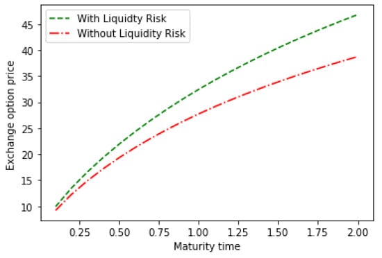
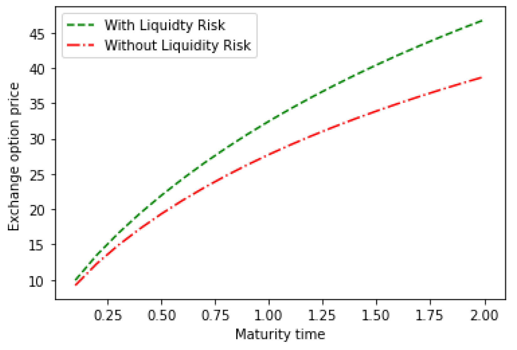
Figure 2 presents the exchange option price for different values of time to maturity. This figure presents the effect of considering stochastic market liquidity against constant market liquidity. The figure depicts that as the maturity time increases, the exchange option price also increases. This can be attributed to the fact that with a longer maturity time, there is an increase in the influence of liquidity, which results in a higher premium. As the maturity time increases from $0.1$ to $2.0$, the option price rises from $9.9840$ to $33.8714$ under constant liquidity and from $10.1484$ to $40.7128$ under the proposed model. Moreover, the gap between the two prices widens with liquidity, increasing from about $0.1644$ at $0.1$ to $6.8415$ at $2.0$, suggesting that the stochastic liquidity leads to higher valuations at a larger maturity time.

Figure 2. Comparison of exchange option price for stochastic market liquidity and constant market liquidity with respect to the range of maturity time $\tau$.

4.1.3. Comparison with Constant Volatility

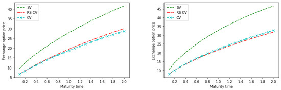
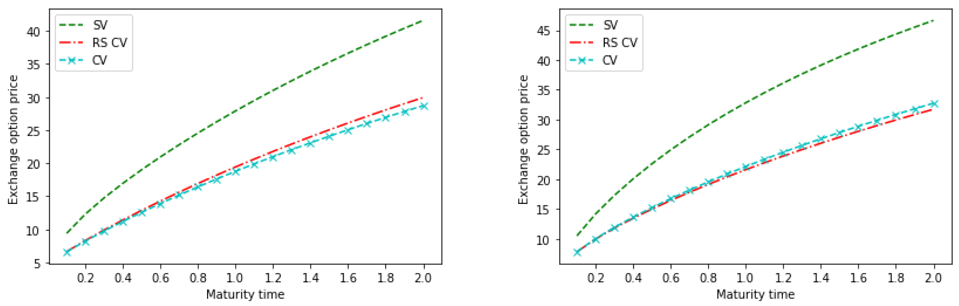
The exchange option prices for various maturity time values are illustrated in Figure 3 in the case of the proposed model, i.e., regime-switching stochastic volatility (SV), regime-switching constant volatility (RS CV) and constant volatility (CV) models. The illustration demonstrates that the exchange option price increases with maturity time for all three cases. In regime-switching stochastic volatility models, option prices are generally higher due to the dynamic nature of volatility as a stochastic process. Quantitatively, the proposed model prices are approximately $42\%$ to $52\%$ higher than the CV prices and about $39\%$ to $49\%$ higher than the RS CV prices across $\tau \in [0.1,2.0]$.

Figure 3. Comparison of exchange option price under the proposed model (SV), RS CV and CV model with respect to a range of maturity time $\tau$ with initial regime 1 (on left) and initial regime 2 (on right).

In the case of the RS CV and CV models, it is observed that in regime 1, the option prices are higher for the RS CV model, whereas for regime 2, the option prices are higher for the CV model. In regime 1, the economy has less risk, resulting in lower option prices. The regime-switching model has a positive probability of transitioning to a different regime. Hence, if the initial regime is regime 1, then the RS CV model can transition to regime 2, a regime with higher risk and hence an increased option price. Similarly, in the case of initial regime 2, the economy can move to regime 1, hence reducing the option price.

4.2. Sensitivity Analysis

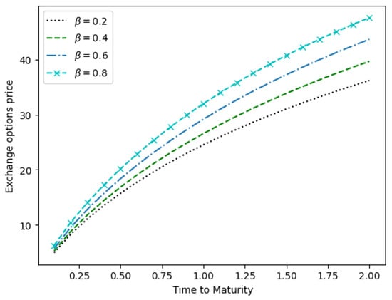
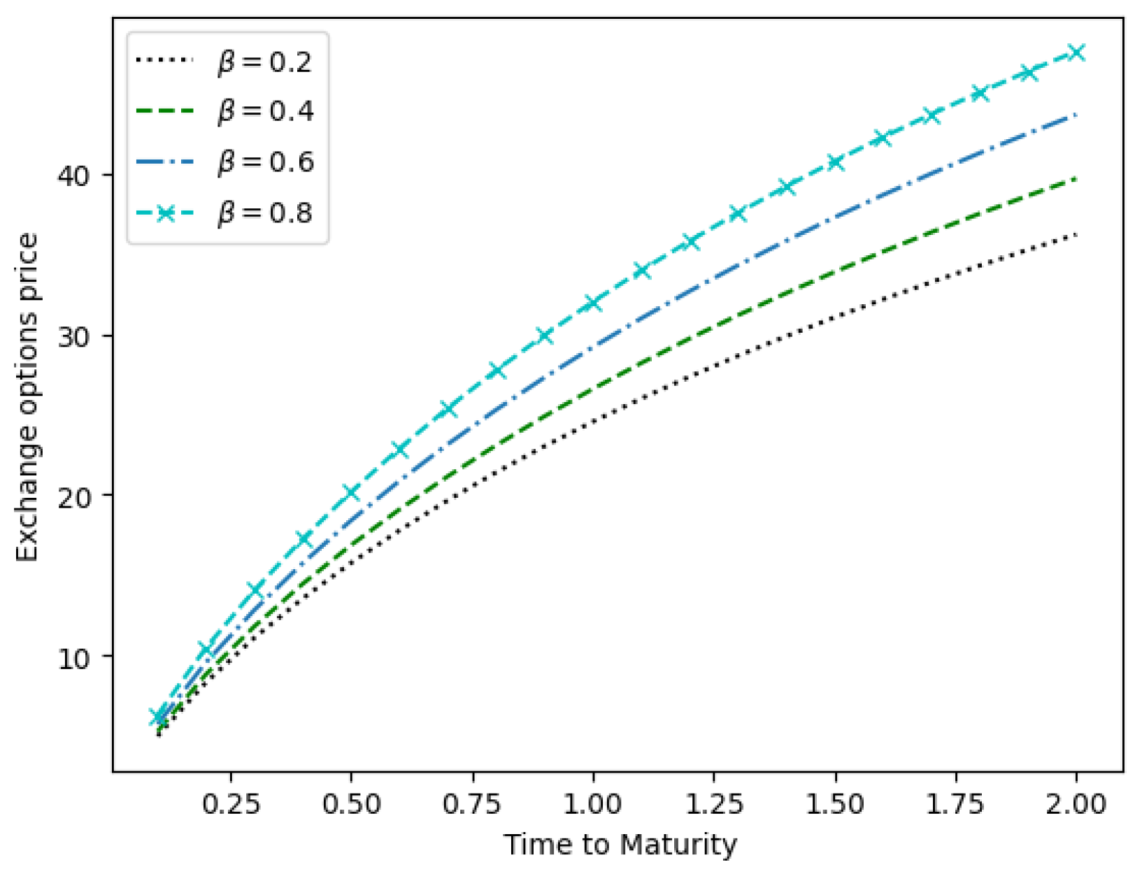
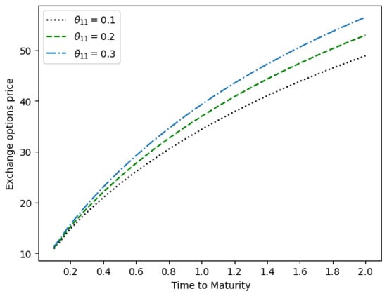
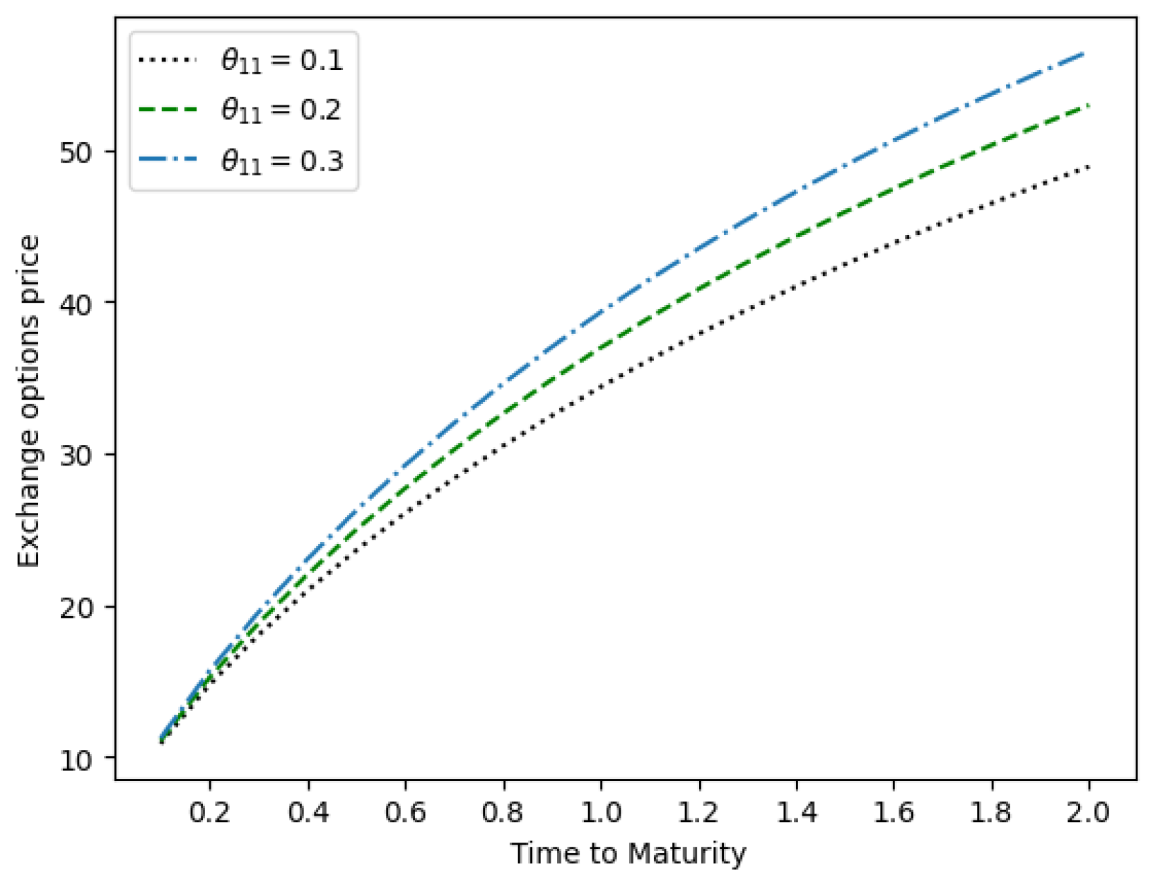
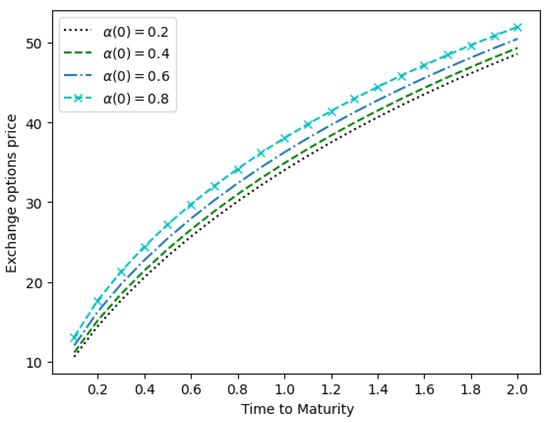
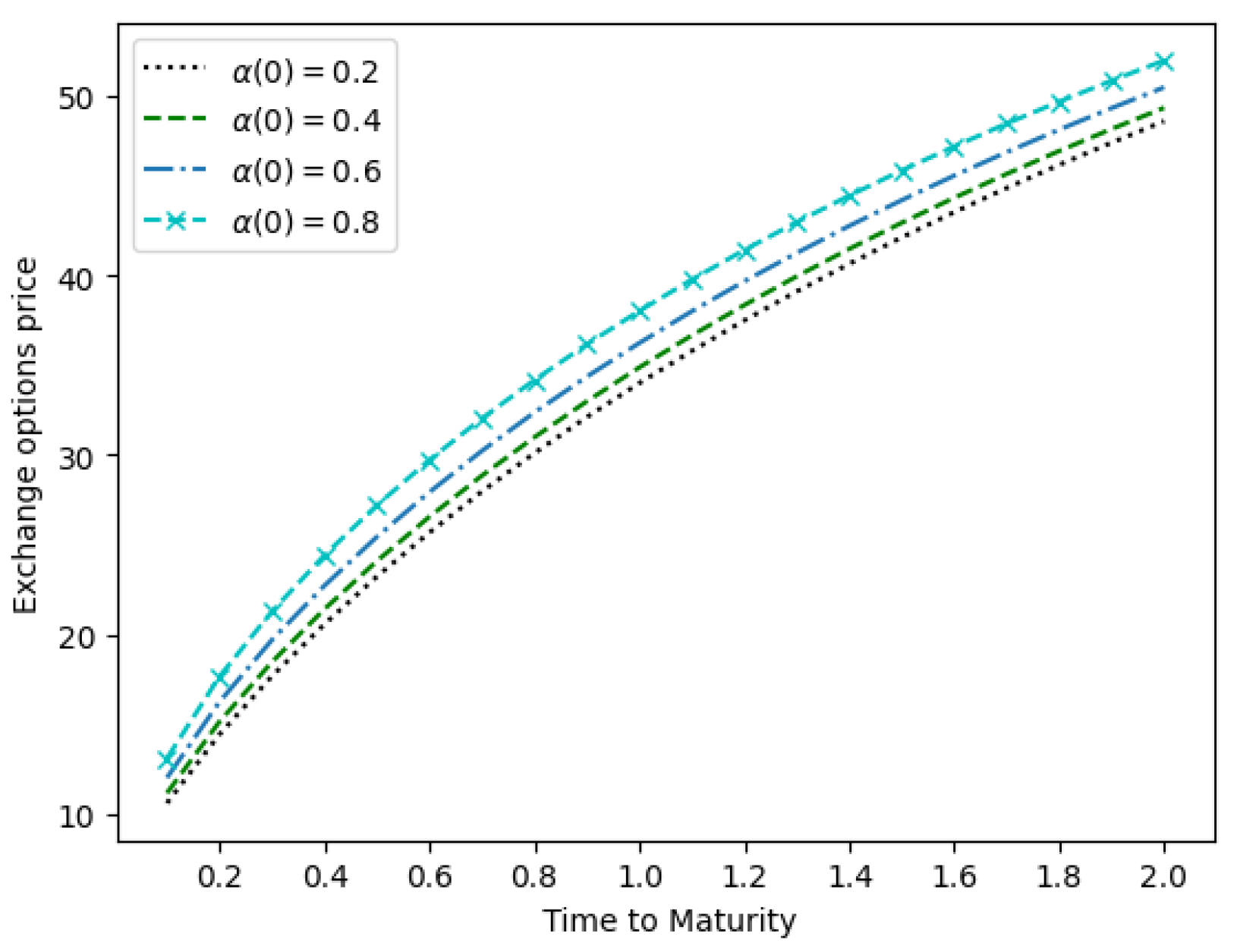
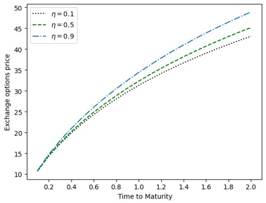
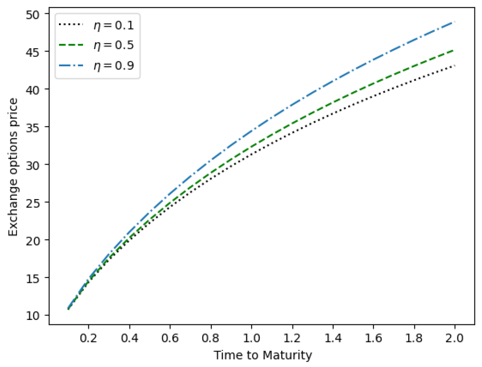
To demonstrate the impact of the asset-specific liquidity parameter ${\beta }_i$ on the exchange option price, it is considered that ${\beta }_1={\beta }_2=\beta$, as shown in Figure 4. It can be observed that the exchange option price is higher when the value of $\beta$ is high. The high value of $\beta$ indicates increased liquidity risk. This graph aligns with the real market scenario, as the reduced liquidity or increased liquidity risk of the assets increases the risk of holding the asset. Therefore, the option writer demands a higher premium in order to mitigate the risk. The impact of liquidity is more pronounced when the maturity time is higher.

Figure 4. Exchange option prices against maturity time for different values of the asset liquidity parameter $\beta$.

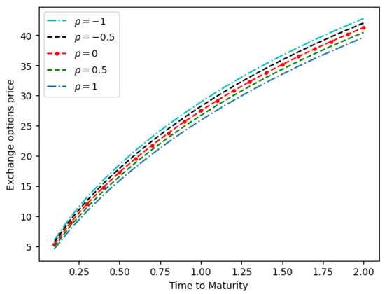
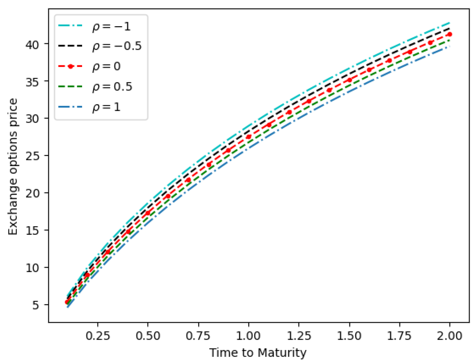
Figure 5 depicts the exchange option price with respect to the time to maturity value. The impact of the correlation coefficient $\rho$ on the option prices can be observed. The exchange option price increases with the increase in the value of the correlation coefficient. This is because if the options have a correlation close to $-1$, then the risk of relative changes in the asset prices is higher in comparison to when they have a correlation close to 1, which results in a higher premium.

Figure 5. Exchange option prices against maturity time for different values of the correlation coefficient between two assets.

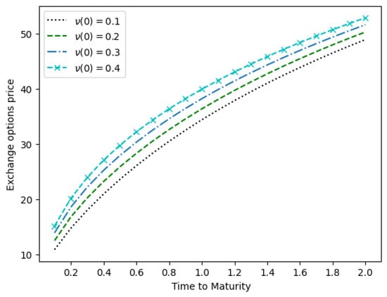
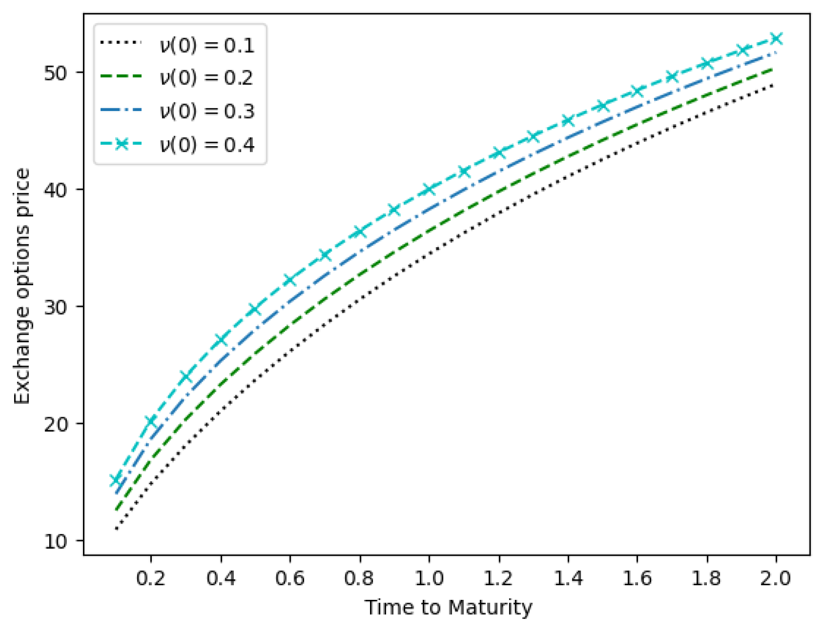
Figure 6 shows the exchange option price for different values of time to maturity. In this figure, it is considered that ${\nu }_1\left(0\right)={\nu }_2\left(0\right)=\nu \left(0\right)$. The figure depicts that as the volatility increases, the exchange option price also increases, as it increases the overall volatility of the assets.

Figure 6. Exchange option prices against maturity time for different values of the initial volatility of the assets.

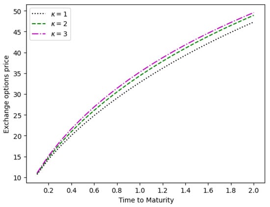
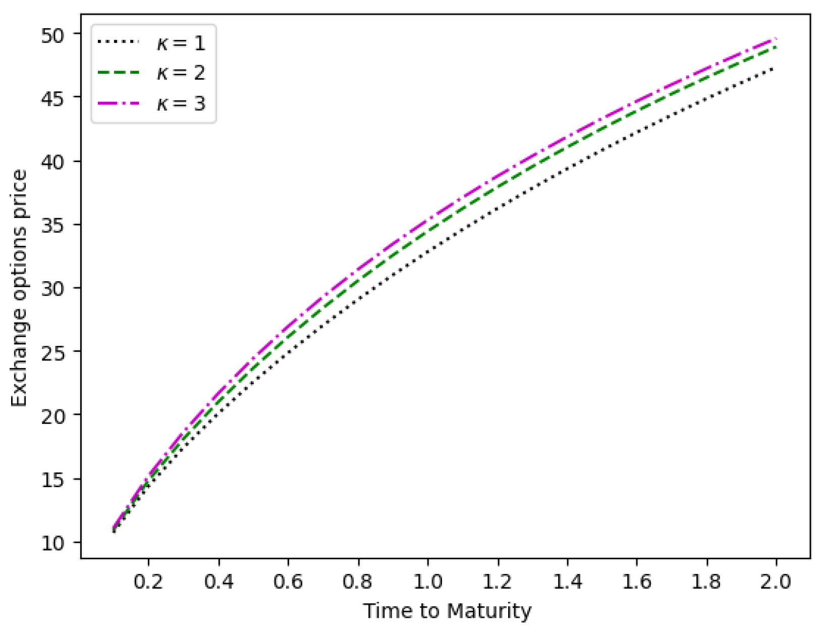
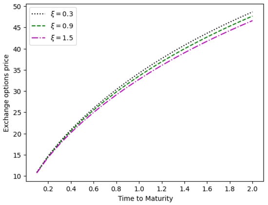
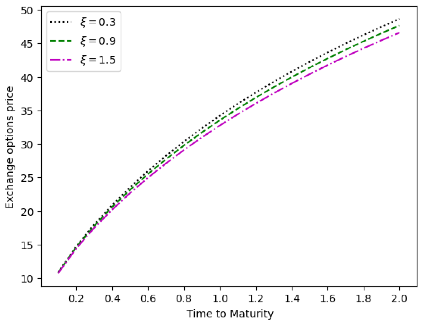
To illustrate the impact of considering stochastic volatility, the exchange option prices across various values of the parameters associated with the stochastic volatility process are investigated against different maturity times. Figure 7 presents the exchange option price for different values of the mean reversion speed $\kappa$ with the assumption that ${\kappa }_1={\kappa }_2=\kappa$. It can be observed that the exchange option price increases with an increase in $\kappa$. Figure 8 shows the exchange option price for different values of maturity time. This figure illustrates the impact of the long-term mean $\theta \left(t\right)$ of volatility with the assumption that ${\theta }_{11}={\theta }_{21}$, ${\theta }_{12}={\theta }_{22}$ and ${\theta }_{11}={\theta }_{12}+0.2$. It is evident from the figure that as the value of ${\theta }_{11}$ increases, the price of the exchange option also increases. With the assumption that ${\xi }_1={\xi }_2=\xi$, the effect of the volatility of volatility $\xi$ on the exchange option price for different values of $\tau$ is depicted in Figure 9. From the figure, it can be observed that as the volatility of volatility increases, the exchange option price decreases.

Figure 7. Exchange option prices against maturity time for different values of ${\kappa }_1={\kappa }_2=\kappa$.

Figure 8. Exchange option prices against maturity time for different values of ${\theta }_{11}={\theta }_{22}+0.2$.

Figure 9. Exchange option prices against maturity time for different values of the ${\xi }_1={\xi }_2=\xi$.

To analyze the impact of the initial value of market liquidity $\alpha \left(0\right)$ on exchange option price, four different values of $\alpha \left(0\right)$ are considered. Figure 10 demonstrates the exchange option price with respect to the ratio of the initial value of assets. It is observed that as the initial value of market liquidity increases, the exchange option price increases. Since, the increase in initial values results in an overall increase in the risk of market liquidity, the exchange option prices are higher.

Figure 10. Exchange option prices against maturity time for different values of initial market liquidity.

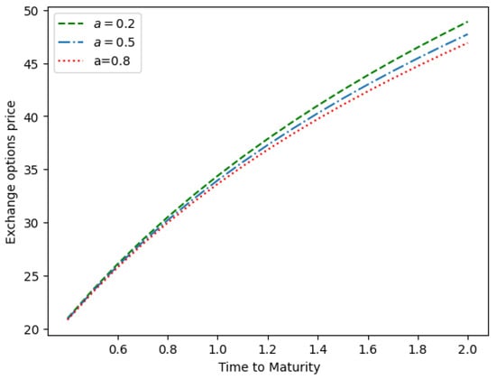
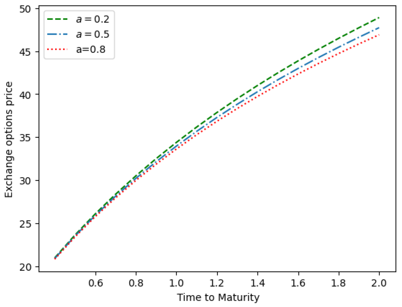
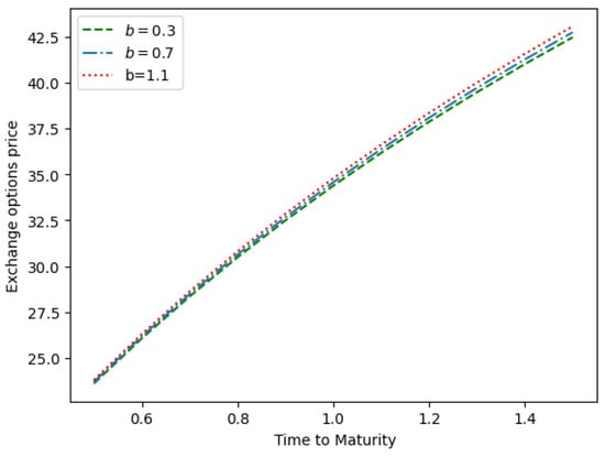
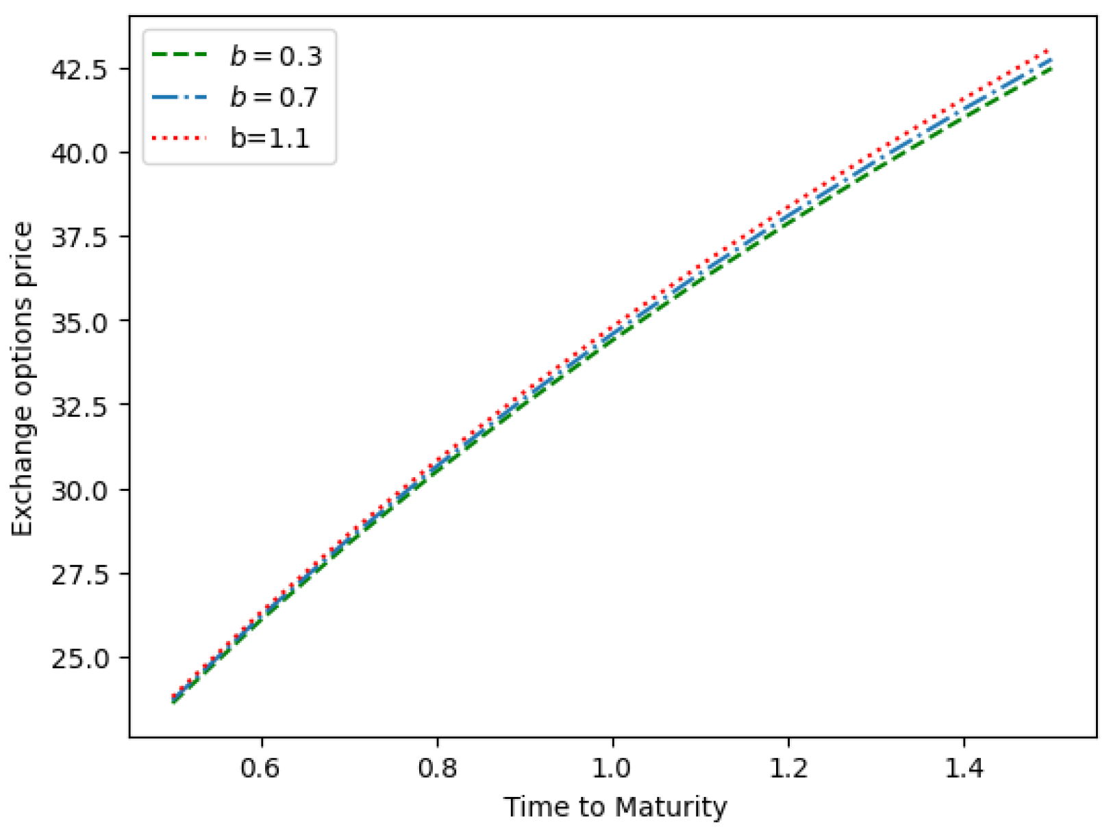
The asset has no liquidity risk if ${\alpha }_i\left(t\right)=0$. For constant values of ${\beta }_i$, a deviation of ${\alpha }_i\left(t\right)$ from 0 indicates that asset i has lower market liquidity. As liquidity diminishes, the risk linked to holding the asset increases, resulting in a higher option premium. Figure 11 illustrates the sensitivity of exchange option prices, influenced by stochastic liquidity and stochastic volatility, to fluctuations in the mean reversion rate $\left(a\right)$ of the market liquidity process $\alpha \left(t\right)$. The price of the exchange option decreases as the value of a increases. This is because the higher values of a indicate that $\alpha \left(t\right)$ will exhibit less fluctuations. Consequently, the option premium decreases. Figure 12 demonstrates the influence of the long-term mean (b) of market liquidity on exchange option valuations. The prices of the exchange option rise with an increase in b. A higher value of b signifies increased long-term illiquidity, leading to higher option prices. Figure 13 depicts the exchange option prices in relation to fluctuations in market liquidity volatility $\left(\eta \right)$. As the $\eta$ value rises, option prices also rise. The increased volatility of $\alpha \left(t\right)$ increases the variations in $\alpha \left(t\right)$, hence increasing the option premium.

Figure 11. Exchange option prices and maturity time for different values of a.

Figure 12. Exchange option prices and maturity time for different values of b.

Figure 13. Exchange option prices and maturity time for different values of $\eta$.

5. Conclusions

This article examines the valuation of European exchange options. The prices of the underlying assets follow the regime-switching model with stochastic volatility, while accounting for liquidity risk effects. The influence of liquidity risk on asset dynamics is represented by a liquidity discount factor that is dependent on both market liquidity and asset-specific liquidity. The pricing formula is obtained through the iterative application of the Feynman–Kac theorem to the proposed model.

To verify the accuracy of the derived formula, comparisons with Monte Carlo simulation outcomes are conducted. Furthermore, sensitivity analysis of various model parameters is performed to demonstrate the impacts of stochastic volatility and liquidity risk. The results indicate that considering regime switching, liquidity risk and stochastic volatility lead to a significant increase in option prices. In this article, jump risk is not considered; one may extend the present framework by modelling jump risk.

There are several directions for future research. First, a dynamic analysis of option prices with $\alpha \left(t\right)$ could be conducted to examine the time-dependent effects on exchange option valuations. Second, comparing payoff distributions across different model specifications could provide deeper insights into the risk characteristics and tail behaviour resulting from regime switching and liquidity effects. Finally, incorporating jump components into asset prices would enable the model to capture sudden market movements, providing a more realistic representation of market dynamics.

References

- Fischer, S. Call option pricing when the exercise price is uncertain, and the valuation of index bonds. J. Financ. 1978, 33, 169–176. [Google Scholar] [CrossRef]
- Margrabe, W. The value of an option to exchange one asset for another. J. Financ. 1978, 33, 177–186. [Google Scholar] [CrossRef]
- Fama, E.F. The behavior of stock-market prices. J. Bus. 1965, 38, 34–105. [Google Scholar] [CrossRef] [Scilit]
- Cont, R. Empirical properties of asset returns: Stylized facts and statistical issues. Quant. Financ. 2001, 1, 223. [Google Scholar] [CrossRef]
- Hull, J.; White, A. The pricing of options on assets with stochastic volatilities. J. Financ. 1987, 42, 281–300. [Google Scholar] [CrossRef]
- Stein, E.M.; Stein, J.C. Stock price distributions with stochastic volatility: An analytic approach. Rev. Financ. Stud. 1991, 4, 727–752. [Google Scholar] [CrossRef] [Scilit]
- Heston, S.L. A closed-form solution for options with stochastic volatility with applications to bond and currency options. Rev. Financ. Stud. 1993, 6, 327–343. [Google Scholar] [CrossRef] [Scilit]
- Acharya, V.V.; Pedersen, L.H. Asset pricing with liquidity risk. J. Financ. Econ. 2005, 77, 375–410. [Google Scholar] [CrossRef] [Scilit]
- Liu, H.; Yong, J. Option pricing with an illiquid underlying asset market. J. Econ. Dyn. Control 2005, 29, 2125–2156. [Google Scholar] [CrossRef] [Scilit]
- Çetin, U.; Jarrow, R.A.; Protter, P. Liquidity risk and arbitrage pricing theory. Financ. Stochastics 2004, 8, 311–341. [Google Scholar] [CrossRef] [Scilit]
- Madan, D.B.; Cherny, A. Markets as a counterparty: An introduction to conic finance. Int. J. Theor. Appl. Financ. 2010, 13, 1149–1177. [Google Scholar] [CrossRef] [Scilit]
- Brunetti, C.; Caldarera, A. Asset Prices and Asset Correlations in Illiquid Markets. SSRN 625184. 2004. Available online: https://papers.ssrn.com/sol3/papers.cfm?abstract_id=625184 (accessed on 31 October 2023).
- Feng, S.P.; Hung, M.W.; Wang, Y.H. Option pricing with stochastic liquidity risk: Theory and evidence. J. Financ. Mark. 2014, 18, 77–95. [Google Scholar] [CrossRef] [Scilit]
- Antonelli, F.; Ramponi, A.; Scarlatti, S. Exchange option pricing under stochastic volatility: A correlation expansion. Rev. Deriv. Res. 2010, 13, 45–73. [Google Scholar] [CrossRef] [Scilit]
- Kim, J.H.; Park, C.R. A multiscale extension of the Margrabe formula under stochastic volatility. Chaos Solitons Fractals 2017, 97, 59–65. [Google Scholar] [CrossRef] [Scilit]
- Cheang, G.H.; Garces, L.P.D.M. Representation of exchange option prices under stochastic volatility jump-diffusion dynamics. Quant. Financ. 2020, 20, 291–310. [Google Scholar] [CrossRef] [Scilit]
- Pasricha, P.; Goel, A. A closed-form pricing formula for European exchange options with stochastic volatility. Probab. Eng. Inf. Sci. 2022, 36, 606–615. [Google Scholar] [CrossRef] [Scilit]
- Carr, P.; Madan, D. Option valuation using the fast Fourier transform. J. Comput. Financ. 1999, 2, 61–73. [Google Scholar] [CrossRef] [Scilit]
- Fang, F.; Oosterlee, C.W. A novel pricing method for European options based on Fourier-cosine series expansions. SIAM J. Sci. Comput. 2009, 31, 826–848. [Google Scholar] [CrossRef] [Scilit]
- Hamilton, J.D. A New Approach to the Economic Analysis of Nonstationary Time Series and the Business Cycle. Econometrica 1989, 57, 357–384. [Google Scholar] [CrossRef] [Scilit]
- Goutte, S.; Ismail, A.; Pham, H. Regime-switching stochastic volatility model: Estimation and calibration to VIX options. Appl. Math. Financ. 2017, 24, 38–75. [Google Scholar] [CrossRef] [Scilit]
- He, X.J.; Lin, S. Analytically pricing exchange options with stochastic liquidity and regime switching. J. Futur. Mark. 2023, 43, 662–676. [Google Scholar] [CrossRef] [Scilit]
- He, X.J.; Lin, S. A stochastic liquidity risk model with stochastic volatility and its applications to option pricing. Stoch. Model. 2024, 41, 273–292. [Google Scholar] [CrossRef] [Scilit]
- Elliott, R.J.; Chan, L.; Siu, T.K. Option pricing and Esscher transform under regime switching. Ann. Financ. 2005, 1, 423–432. [Google Scholar] [CrossRef] [Scilit]
- Feng, S.P.; Hung, M.W.; Wang, Y.H. The importance of stock liquidity on option pricing. Int. Rev. Econ. Financ. 2016, 43, 457–467. [Google Scholar] [CrossRef] [Scilit]
- Mittal, P.; Selvamuthu, D. Vulnerable power exchange options with liquidity risk. Phys. A Stat. Mech. Its Appl. 2025, 672, 130646. [Google Scholar] [CrossRef] [Scilit]
- Mittal, P.; Selvamuthu, D. Options pricing with Markov regime switching Heston volatility Hull–White interest rates and stochastic intensity. Probab. Eng. Inf. Sci. 2025, 39, 243–259. [Google Scholar] [CrossRef] [Scilit]
- Duffie, D.; Pan, J.; Singleton, K. Transform analysis and asset pricing for affine jump-diffusions. Econometrica 2000, 68, 1343–1376. [Google Scholar] [CrossRef] [Scilit]
- Elliott, R.J.; Nishide, K. Pricing of discount bonds with a Markov switching regime. Ann. Financ. 2014, 10, 509–522. [Google Scholar] [CrossRef] [Scilit]
- Pasricha, P.; He, X.J. Exchange options with stochastic liquidity risk. Expert Syst. Appl. 2023, 223, 119915. [Google Scholar] [CrossRef] [Scilit]
Disclaimer/Publisher’s Note: The statements, opinions and data contained in all publications are solely those of the individual author(s) and contributor(s) and not of MDPI and/or the editor(s). MDPI and/or the editor(s) disclaim responsibility for any injury to people or property resulting from any ideas, methods, instructions or products referred to in the content. |
© 2026 by the authors. Licensee MDPI, Basel, Switzerland. This article is an open access article distributed under the terms and conditions of the Creative Commons Attribution (CC BY) license.