Optimal Control for Linearized Non-Isentropic Compressible Navier–Stokes Equations

Abstract

This paper investigates the optimal control problem for the non-isentropic compressible Navier–Stokes equations linearized around a constant steady state. First, we establish estimates for the solution of the state equation. Then, we prove the existence and uniqueness of the optimal control, derive the necessary optimality conditions, and obtain an explicit characterization of the control via the optimality system. Finally, we present a numerical experiment to compute the control using the derived formula.

1. Introduction

As is known, the Navier–Stokes system in $\mathrm{\Omega }\subset {\mathbb{R}}^N$ for a compressible non-isentropic fluid consists of the mass conservation equation

$${\rho }_t+\mathrm{d}\mathrm{i}\mathrm{v}\left(\rho \mathbf{u}\right)=0,$$

the momentum conservation equation

$$\rho ({\mathbf{u}}_t+(\mathbf{u}·\nabla )\mathbf{u})+\nabla P(\rho ,\theta )=\mu ▵\mathbf{u}+(\mu +\lambda )\nabla \mathrm{d}\mathrm{i}\mathrm{v}\mathrm{u}+\rho \mathbf{f},$$

and the energy conservation equation

$$\rho C_v({\theta }_t+\mathbf{u}·\nabla \theta )+\theta P_{\theta }(\rho ,\theta )\mathrm{d}\mathrm{i}\mathrm{v}\mathbf{u}=\kappa ▵\theta +\lambda {\left(\mathrm{d}\mathrm{i}\mathrm{v}\mathbf{u}\right)}^2+{\displaystyle \frac{\mu }{2}}\sum _{i,j=1}^N{({𝜕}_i{u}_j+{𝜕}_j{u}_i)}^2,$$

where $\rho (x,t)$, $\mathbf{u}(x,t)$, and $\theta (x,t)$ are the density, velocity, and temperature of the fluid, respectively, $\mathbf{f}$ is an external force, $\mu$ and $\lambda$ are the viscosity coefficients satisfying the restrictions $\mu >0$ and $\lambda +{\displaystyle \frac{2}{3}}\mu >0$, $C_v$ is the specific heat constant, $\kappa$ is the heat conductivity constant, and P is the pressure given by the ideal gas law

$$P(\rho ,\theta )=R\rho \theta$$

with R being the universal gas constant.

In this paper, we consider one-dimensional Navier–Stokes equations linearized around a constant steady state $(0,V_0,H_0)$ in a bounded interval $(0,1)$ with $V_0>0$ and $H_0\ge 0$. Precisely, consider the system    

$$\begin{array}{c}\hfill \left\{\begin{array}{cc}{\rho }_t+V_0{v}_x=0,\hfill & (x,t)\in Q_T,\hfill \\ v_t-{\displaystyle \frac{\lambda +2\mu }{V_0}}{v}_{xx}+{\displaystyle \frac{R{H}_0}{V_0}}{\rho }_x+R{\theta }_x=g{\chi }_{\omega },\hfill & (x,t)\in Q_T,\hfill \\ {\theta }_t-{\displaystyle \frac{\kappa }{V_0{c}_v}}{\theta }_{xx}+{\displaystyle \frac{R{H}_0}{c_v}}{v}_x=0,\hfill & (x,t)\in Q_T,\hfill \\ v(0,t)=v(1,t)=\theta (0,t)=\theta (1,t)=0,\hfill & t\in (0,T),\hfill \\ \rho (x,0)={\rho }_0\left(x\right),v(x,0)=v_0\left(x\right),\theta (x,0)={\theta }_0\left(x\right),\hfill & x\in (0,1),\hfill \end{array}\right.\end{array}$$

(1)

where $\omega$ is a subset of $(0,1)$, ${\chi }_{\omega }$ is the characteristic function on $\omega$, and $Q_T=(0,1)\times (0,T)$.

In this paper, we are concerned with the following optimal control problem:

$$\begin{array}{c}\begin{array}{cc}\hfill \left(P\right)\underset{f\in U_{ad}}{min}J\left(g\right)=& {\displaystyle \frac{1}{2}}{\int }_0^T{\int }_0^1{g}^{2}dxdt+{\displaystyle \frac{{\lambda }_1}{2}}{\int }_0^1{(\rho (x,T)-{\rho }_d\left(x\right))}^{2}dx\hfill \\ & +{\displaystyle \frac{{\lambda }_2}{2}}{\int }_0^1{(v(x,T)-v_d\left(x\right))}^{2}dx+{\displaystyle \frac{{\lambda }_3}{2}}{\int }_0^1{(\theta (x,T)-{\theta }_d\left(x\right))}^{2}dx,\hfill \end{array}\end{array}$$

where ${\lambda }_1,{\lambda }_2,{\lambda }_3>0$, ${(\rho ,v,\theta )}^{\top }$ is the solution of Equation (1), ${({\rho }_d,v_d,{\theta }_d)}^{\top }$ is the value expected to be achieved at time t, and

$$U_{ad}=\{g\in L^2\left(Q_T\right):g(x,t)=0,(x,t)\in \left((0,1)\setminus \omega \right)\times (0,T)\mathrm{and}\mathrm{supp}g\subset \omega \times (0,T)\}.$$

The optimal control problems for the non-isentropic compressible Navier–Stokes equations is valuable in practical applications such as aerospace and thermal systems. In aerospace, it helps regulate flows in hypersonic vehicles and turbine combustors to reduce thermal loads, improve combustion efficiency, and enhance stability. In thermal control, the model aids in designing efficient controllers for real-time thermal management of critical equipment. Optimal control of Navier–Stokes equations has been a topic of extensive research. For incompressible fluids, the work on optimal control is extensive. Desai and Ito [1] studied optimal control problems of fluid flow governed by the Navier–Stokes equations, focusing on the cases of a driven cavity and flow through a channel with sudden expansion. Ghattas and Bark [2] developed numerical optimization methods for optimal control of steady incompressible Navier–Stokes flows. Roubíček and Tröltzsch [3] explored Lipschitz stability in optimal controls for steady-state solutions. Wang [4] applied Pontryagin’s maximum principle to the stationary equations, while De Los Reyes and Tröltzsch [5] considered mixed control-state constraints in the stationary case. De Los Reyes and Griesse [6] focused on state-constrained optimal control for three-dimensional flows. Recently, research has extended to the Cahn–Hilliard–Navier–Stokes system [7], infinite horizon Navier–Stokes equations [8], a 3D-chemotaxis-Navier–Stokes model [9], and so on. Isentropic compressible Navier–Stokes equations have been featured in a few papers in recent years. Doboszczak et al. [10] investigated the existence of the optimal controls in three dimensions. Chowdhury and Ramaswamy [11] studied an optimal boundary control for the linearized compressible Navier–Stokes equations. Doboszczak et al. [12] applied Pontryagin’s principle to state-constrained linearized Navier–Stokes equations.

Notably, advances from fractional calculus and iterative learning control also enrich relevant research tools. Ref. [13] explores the solution properties of fractional equations with nonlocal boundary conditions, providing a mathematical basis for flow models involving nonlocal interactions. Ref. [14] proposes a P-type iterative learning control method for fractional derivative pulse-variable systems, verifying its effectiveness in complex dynamical system tracking—useful for optimizing flow control strategies.

Although Maity [15] has established null controllability for the non-isentropic compressible Navier–Stokes equations linearized around a constant steady state, the corresponding optimal control problem remains completely unexplored. The present work is directly motivated by this gap. In this paper, we study the optimal control problem $\left(P\right)$ governed by the linearized non-isentropic compressible Navier–Stokes Equation (1). First, we establish the well-posedness of System (1) and derive necessary estimates. Next, we prove the existence of an optimal control, derive the first-order necessary condition, obtain an explicit formula for the optimal control from the optimality system, and prove its uniqueness. Finally, we present a numerical experiment to compute the optimal control using this formula.

The paper is organized as follows: In Section 2, we introduce some results on the well-posedness of Navier–Stokes equations and establish the estimates for the solution. In Section 3, we prove the existence and uniqueness of the optimal control and derive the necessary condition for the optimal control. In Section 4, we provide a numerical experiment to solve the optimal control problem. In Section 5, we conclude the paper and discuss potential future research directions.

2. Well-Posedness of the Linearized Navier–Stokes Equations

In this section, we introduce the well-posedness of the linearized Navier–Stokes system (1) and establish the estimates for it.

Let $B=L^2(0,1)\times L^2(0,1)\times L^2(0,1)$ be a Hilbert space. Define an unbounded operator $(A,D(A\left)\right)$ on B, where

$$A=\left(\begin{array}{ccc}0& V_0{\displaystyle \frac{d}{dx}}& 0\\ {\displaystyle \frac{R{H}_0}{V_0}}{\displaystyle \frac{d}{dx}}& -{\displaystyle \frac{\lambda +2\mu }{V_0}}{\displaystyle \frac{d^2}{d{x}^2}}& R{\displaystyle \frac{d}{dx}}\\ 0& {\displaystyle \frac{R{H}_0}{c_v}}{\displaystyle \frac{d}{dx}}& -{\displaystyle \frac{\kappa }{V_0{c}_v}}{\displaystyle \frac{d^2}{d{x}^2}}\end{array}\right)$$

and

$$D\left(A\right)=\left\{{(\sigma ,u,\varphi )}^{\top }\in B:\sigma \in H^1(0,1),u\in H_0^1(0,1)\cap H^2(0,1),\varphi \in H_0^1(0,1)\cap H^2(0,1)\right\}.$$

The following lemma can be obtained using semigroup theory (see [16]).

Lemma 1. 

Let $(-A,D(A\left)\right)$ be a strongly continuous contraction semigroup on B. For each ${({\rho }_0,v_0,{\theta }_0)}^{\top }\in B$, Problem (1) has a unique solution ${(\rho ,v,\theta )}^{\top }$ satisfying the following properties:

(1)

if ${(\rho ,v,\theta )}^{\top }\in B$, $g\in L^2\left(Q_T\right)$, then ${(\rho ,v,\theta )}^{\top }\in C\left([0,T];B\right)$ and

$${\parallel (\rho ,v,\theta )\parallel }_{C\left(\right[0,T],B)}\le {\parallel ({\rho }_0,v_0,{\theta }_0)\parallel }_B+C{\parallel g\parallel }_{L^2\left(Q_T\right)};$$

(2)

if ${({\rho }_0,v_0,{\theta }_0)}^{\top }\in D\left(A\right)$, $g\in C\left([0,T];H_0^1\left(\mathrm{\Omega }\right)\cap H^2\left(\mathrm{\Omega }\right)\right)$, then

$$(\rho ,v,\theta )\in C\left([0,T],D\left(A\right)\right)\cap H^1\left(0,T;B\right).$$

Definition 1. 

We say that $(\rho ,v,\theta )\in C\left([0,T];B\right)$ with $v,\theta \in L^2\left([0,T];H_0^1(0,1)\right)$ is a weak solution to Equation (1), if for any $(\psi ,\varphi ,\phi )\in C\left([0,T],D\left(A\right)\right)\cap H^1\left(0,T;B\right)$, the following integral equalities hold:    

$$\begin{array}{cc}\hfill & {\int \int }_{Q_T}(-\rho {\psi }_t+V_0{v}_x\psi )dxdt=-{\int }_0^1\left(\rho (x,T)\psi (x,T)-{\rho }_0\left(x\right)\psi (x,0)\right)dx,\hfill \\ \hfill & {\int \int }_{Q_T}\left(-v{\varphi }_t+{\displaystyle \frac{\lambda +2\mu }{V_0}}{v}_x{\varphi }_x-{\displaystyle \frac{R{H}_0}{V_0}}\rho {\varphi }_x+R{\theta }_x{\varphi }_x\right)dxdt\hfill \\ \hfill =& {\int \int }_{Q_T}g\varphi dxdt-{\int }_0^1\left(v(x,T)\varphi (x,T)-v_0\left(x\right)\varphi (x,0)\right)dx,\hfill \\ \hfill & {\int \int }_{Q_T}\left(-\theta {\phi }_t+{\displaystyle \frac{\kappa }{V_0{c}_v}}{\theta }_x{\phi }_x-{\displaystyle \frac{R{H}_0}{c_v}}v{\phi }_x\right)dxdt\hfill \\ \hfill =& -{\int }_0^1\left(\theta (x,T)\phi (x,T)-{\theta }_0\left(x\right)\phi (x,0)\right)dx.\hfill \end{array}$$

Theorem 1. 

For any ${({\rho }_0,v_0,{\theta }_0)}^{\top }\in B$, $g\in L^2\left(Q_T\right)$, Problem (1) admits a unique weak solution ${(\rho ,v,\theta )}^{\top }\in C\left([0,T];B\right)$, and $({\rho }_t,v_t,{\theta }_t)\in L^2(0,T;H^{-1}(0,1))$. Furthermore, the following estimate holds:

$$\begin{array}{cc}\hfill & {\parallel \rho \parallel }_{L^{\infty }(0,T;L^2(0,1))}+{\parallel v\parallel }_{L^{\infty }(0,T;L^2(0,1))}+{\parallel \theta \parallel }_{L^{\infty }(0,T;L^2(0,1))}\hfill \\ \hfill & +{\parallel {\rho }_t\parallel }_{L^{\infty }(0,T;H^{-1}(0,1))}+{\parallel v_t\parallel }_{L^{\infty }(0,T;H^{-1}(0,1))}+{\parallel {\theta }_t\parallel }_{L^{\infty }(0,T;H^{-1}(0,1))}\hfill \\ \hfill & +{\parallel v\parallel }_{L^2(0,T;H^1(0,1))}+{\parallel \theta \parallel }_{L^2(0,T;H^1(0,1))}\hfill \\ \hfill \le & C\left({\parallel g\parallel }_{{\left(L^2\left(Q_T\right)\right)}^3}+{\parallel {\rho }_0\parallel }_{L^2(0,1)}+{\parallel v_0\parallel }_{L^2(0,1)}+{\parallel {\theta }_0\parallel }_{L^2(0,1)}\right),\hfill \end{array}$$

(2)

where $C>0$ is a constant. Here, $H^{-1}(0,1)$ denotes the dual space of $H_0^1(0,1)$.

Proof. 

For any ${(\rho ,v,\theta )}^{\top }\in {\left(L^2(0,1)\right)}^3$, $g\in L^2\left(Q_T\right)$, there are sequences ${\left\{{\rho }_0^{\left(n\right)}\right\}}_{n=1}^{\infty }\subset C_0^{\infty }(0,1)$, ${\left\{v_0^{\left(n\right)}\right\}}_{n=1}^{\infty }\subset C_0^{\infty }(0,1)$, ${\left\{{\theta }_0^{\left(n\right)}\right\}}_{n=1}^{\infty }\subset C_0^{\infty }(0,1)$, ${\left\{g^{\left(n\right)}\right\}}_{n=1}^{\infty }\subset C_0^{\infty }\left(Q_T\right)$ with $g^{\left(n\right)}\subset \omega \times (0,T)$, such that

$$\begin{array}{cc}\hfill & {\parallel {\rho }_0^{\left(n\right)}\parallel }_{L^2(0,1)}\le 2{\parallel {\rho }_0\parallel }_{L^2(0,1)},{\parallel v_0^{\left(n\right)}\parallel }_{L^2(0,1)}\le 2{\parallel v_0\parallel }_{L^2(0,1)},\hfill \\ \hfill & {\parallel {\theta }_0^{\left(n\right)}\parallel }_{L^2(0,1)}\le 2{\parallel {\theta }_0\parallel }_{L^2(0,1)},{\parallel g^{\left(n\right)}\parallel }_{L^2\left(Q_T\right)}\le 2{\parallel g\parallel }_{L^2\left(Q_T\right)}\hfill \end{array}$$

(3)

and

$$\begin{array}{cc}\hfill & {\rho }_0^{\left(n\right)}\to {\rho }_0,v_0^{\left(n\right)}\to v_0,{\theta }_0^{\left(n\right)}\to {\theta }_0\mathrm{in}{L}^2(0,1),g^{\left(n\right)}\to g\mathrm{in}{L}^2\left(Q_T\right),\mathrm{as}n\to \infty .\hfill \end{array}$$

(4)

Now, consider the following problem:

$$\begin{array}{c}\begin{array}{c}\hfill \left\{\begin{array}{cc}{\rho }_t^{\left(n\right)}+V_0{v}_x^{\left(n\right)}=0,\hfill & (x,t)\in Q_T,\hfill \\ v_t^{\left(n\right)}-{\displaystyle \frac{\lambda +2\mu }{V_0}}{v}_{xx}^{\left(n\right)}+{\displaystyle \frac{R{H}_0}{V_0}}{\rho }_x^{\left(n\right)}+R{\theta }_x^{\left(n\right)}=g^{\left(n\right)},\hfill & (x,t)\in Q_T,\hfill \\ {\theta }_t^{\left(n\right)}-{\displaystyle \frac{\kappa }{V_0{c}_v}}{\theta }_{xx}^{\left(n\right)}+{\displaystyle \frac{R{H}_0}{c_v}}{v}_x^{\left(n\right)}=0,\hfill & (x,t)\in Q_T,\hfill \\ v^{\left(n\right)}(0,t)=v^{\left(n\right)}(1,t)={\theta }^{\left(n\right)}(0,t)={\theta }^{\left(n\right)}(1,t)=0,\hfill & t\in (0,T),\hfill \\ {\rho }^{\left(n\right)}(x,0)={\rho }_0\left(x\right),v^{\left(n\right)}(x,0)=v_0\left(x\right),{\theta }^{\left(n\right)}(x,0)={\theta }_0\left(x\right),\hfill & x\in (0,1).\hfill \end{array}\right.\end{array}\end{array}$$

(5)

From Lemma 1 (2), the problem admits a unique solution ${(\rho ,v,\theta )}^{\top }\in C\left([0,T],D\left(A\right)\right)\cap H^1\left(0,T;B\right)$. By multiplying the first equation of (5) by ${\rho }^{\left(n\right)}$ and then integrating by parts over $(0,1)\times (0,t)$, we obtain

$$\begin{array}{c}\hfill {\displaystyle \frac{1}{2}}{\int }_{\mathrm{\Omega }}{\left({\rho }^{\left(n\right)}\right)}^2(x,t)dx={\displaystyle \frac{1}{2}}{\int }_{\mathrm{\Omega }}{\left({\rho }_0^{\left(n\right)}\right)}^2\left(x\right)dx-V_0{\int }_0^t{\int }_{\mathrm{\Omega }}\left(v_x^{\left(n\right)}{\rho }^{\left(n\right)}\right)(x,s)dx.\end{array}$$

(6)

By multiplying the second equation of (5) by $v^{\left(n\right)}$ and then integrating by parts over $(0,1)\times (0,t)$, we obtain    

$$\begin{array}{cc}\hfill & {\displaystyle \frac{1}{2}}{\int }_{\mathrm{\Omega }}{\left(v^{\left(n\right)}\right)}^2(x,t)dx+{\displaystyle \frac{\lambda +2\mu }{V_0}}{\int }_0^t{\int }_{\mathrm{\Omega }}{\left(v_x^{\left(n\right)}\right)}^2(x,s)dxds\hfill \\ \hfill =& {\displaystyle \frac{1}{2}}{\int }_{\mathrm{\Omega }}{\left(v_0^{\left(n\right)}\right)}^2\left(x\right)dx+{\int }_0^t{\int }_{\mathrm{\Omega }}\left(g^{\left(n\right)}{v}^{\left(n\right)}\right)(x,s)dxds-{\displaystyle \frac{R{H}_0}{V_0}}{\int }_0^t{\int }_{\mathrm{\Omega }}({\rho }^{\left(n\right)}{v}_x^{\left(n\right)})(x,s)dxds\hfill \\ \hfill & +R{\int }_0^t{\int }_{\mathrm{\Omega }}\left({\theta }^{\left(n\right)}{v}_x^{\left(n\right)}\right)(x,s)dxds.\hfill \end{array}$$

(7)

By multiplying the third equation of (5) by ${\theta }^{\left(n\right)}$ and then integrating by parts over $(0,1)\times (0,t)$, we obtain

$$\begin{array}{cc}\hfill & {\displaystyle \frac{1}{2}}{\int }_{\mathrm{\Omega }}{\left({\theta }^{\left(n\right)}\right)}^2(x,t)dx+{\displaystyle \frac{\kappa }{V_0{c}_v}}{\int }_0^t{\int }_{\mathrm{\Omega }}{\left({\theta }_x^{\left(n\right)}\right)}^2(x,s)dxds\hfill \\ \hfill =& {\displaystyle \frac{1}{2}}{\int }_{\mathrm{\Omega }}{\left({\theta }_0^{\left(n\right)}\right)}^2\left(x\right)dx-{\displaystyle \frac{R{H}_0}{c_v}}{\int }_0^t{\int }_{\mathrm{\Omega }}\left(v^{\left(n\right)}{\theta }_x^{\left(n\right)}\right)(x,s)dxds.\hfill \end{array}$$

(8)

Combining (6)–(8), we obtain

$$\begin{array}{cc}\hfill & {\displaystyle \frac{1}{2}}{\int }_0^1{\left({\rho }^{\left(n\right)}\right)}^2(x,t)dx+{\displaystyle \frac{1}{2}}{\int }_0^1{\left(v^{\left(n\right)}\right)}^2(x,t)dx+{\displaystyle \frac{1}{2}}{\int }_0^1{\left({\theta }^{\left(n\right)}\right)}^2(x,t)dx\hfill \\ \hfill & +{\displaystyle \frac{\lambda +2\mu }{V_0}}{\int }_0^t{\int }_0^1{\left(v_x^{\left(n\right)}\right)}^2(x,s)dxds+{\displaystyle \frac{\kappa }{V_0{c}_v}}{\int }_0^t{\int }_0^1{\left({\theta }_x^{\left(n\right)}\right)}^2(x,s)dxds\hfill \\ \hfill \le & {\displaystyle \frac{1}{2}}{\int }_0^1{\left({\rho }_0^{\left(n\right)}\right)}^2\left(x\right)dx+{\displaystyle \frac{1}{2}}{\int }_0^1{\left(v_0^{\left(n\right)}\right)}^2\left(x\right)dx+{\displaystyle \frac{1}{2}}{\int }_0^1{\left({\theta }_0^{\left(n\right)}\right)}^2\left(x\right)dx\hfill \\ \hfill & +{\displaystyle \frac{1}{2}}{\int }_0^t{\int }_0^1{\left(g^{\left(n\right)}\right)}^2(x,s)dxds+{\displaystyle \frac{\lambda +2\mu }{2V_0}}{\int }_0^t{\int }_0^1{\left(v_x^{\left(n\right)}\right)}^2(x,s)dxds\hfill \\ \hfill & +{\displaystyle \frac{\kappa }{2V_0{c}_v}}{\int }_0^t{\int }_0^1{\left({\theta }_x^{\left(n\right)}\right)}^2(x,s)dxds+C_1({\int }_0^t{\int }_0^1{\left({\rho }^{\left(n\right)}\right)}^2(x,s)dxds\hfill \\ \hfill & +{\int }_0^t{\int }_0^1{\left(v^{\left(n\right)}\right)}^2(x,s)dxds+{\int }_0^t{\int }_0^1{\left({\theta }^{\left(n\right)}\right)}^2(x,s)dxds),\hfill \end{array}$$

where $C_1>0$ is a constant. Therefore,

$$\begin{array}{cc}\hfill & {\int }_0^1{\left({\rho }^{\left(n\right)}\right)}^2(x,t)dx+{\int }_0^1{\left(v^{\left(n\right)}\right)}^2(x,t)dx+{\int }_0^1{\left({\theta }^{\left(n\right)}\right)}^2(x,t)dx\hfill \\ \hfill & +{\displaystyle \frac{\lambda +2\mu }{V_0}}{\int }_0^t{\int }_0^1{\left(v_x^{\left(n\right)}\right)}^2(x,s)dxds+{\displaystyle \frac{\kappa }{V_0{c}_v}}{\int }_0^t{\int }_0^1{\left({\theta }_x^{\left(n\right)}\right)}^2(x,s)dxds\hfill \\ \hfill \le & {\int }_0^1{\left({\rho }_0^{\left(n\right)}\right)}^2\left(x\right)dx+{\int }_0^1{\left(v_0^{\left(n\right)}\right)}^2\left(x\right)dx+{\int }_0^1{\left({\theta }_0^{\left(n\right)}\right)}^2\left(x\right)dx\hfill \\ \hfill & +{\int }_0^t{\int }_0^1{\left(g^{\left(n\right)}\right)}^2(x,s)dxds+2C_1({\int }_0^t{\int }_0^1{\left({\rho }^{\left(n\right)}\right)}^2(x,s)dxds\hfill \\ \hfill & +{\int }_0^t{\int }_0^1{\left(v^{\left(n\right)}\right)}^2(x,s)dxds+{\int }_0^t{\int }_0^1{\left({\theta }^{\left(n\right)}\right)}^2(x,s)dxds).\hfill \end{array}$$

Using Gronwall’s inequality and (3), we have

$$\begin{array}{cc}\hfill & {\int }_0^1{\left({\rho }^{\left(n\right)}\right)}^2(x,t)dx+{\int }_0^1{\left(v^{\left(n\right)}\right)}^2(x,t)dx+{\int }_0^1{\left({\theta }^{\left(n\right)}\right)}^2(x,t)dx\hfill \\ \hfill & +{\displaystyle \frac{\lambda +2\mu }{V_0}}{\int }_0^t{\int }_0^1{\left(v_x^{\left(n\right)}\right)}^2(x,s)dxds+{\displaystyle \frac{\kappa }{V_0{c}_v}}{\int }_0^t{\int }_0^1{\left({\theta }_x^{\left(n\right)}\right)}^2(x,s)dxds\hfill \\ \hfill \le & e^{2C_{1}T}\left({\int }_0^1{\left({\rho }_0^{\left(n\right)}\right)}^2\left(x\right)dx+{\int }_0^1{\left(v_0^{\left(n\right)}\right)}^2\left(x\right)dx+{\int }_0^1{\left({\theta }_0^{\left(n\right)}\right)}^2\left(x\right)dx+{\int }_0^t{\int }_0^1{\left(g^{\left(n\right)}\right)}^2(x,s)dxds\right)\hfill \\ \hfill \le & 4e^{2C_{1}T}\left({\int }_0^1{\left({\rho }_0\right)}^2\left(x\right)dx+{\int }_0^1{\left(v_0\right)}^2\left(x\right)dx+{\int }_0^1{\left({\theta }_0\right)}^2\left(x\right)dx+{\int }_0^t{\int }_0^1{\left(g\right)}^2(x,s)dxds\right),\hfill \end{array}$$

which implies

$$\begin{array}{cc}\hfill & \underset{0\le t\le T}{sup}{\int }_0^1{\left({\rho }^{\left(n\right)}\right)}^2(x,t)dx+\underset{0\le t\le T}{sup}{\int }_0^1{\left(v^{\left(n\right)}\right)}^2(x,t)dx+\underset{0\le t\le T}{sup}{\int }_0^1{\left({\theta }^{\left(n\right)}\right)}^2(x,t)dx\hfill \\ \hfill & +{\displaystyle \frac{\lambda +2\mu }{V_0}}{\int }_0^t{\int }_0^1{\left(v_x^{\left(n\right)}\right)}^2(x,s)dxds+{\displaystyle \frac{\kappa }{V_0{c}_v}}{\int }_0^t{\int }_0^1{\left({\theta }_x^{\left(n\right)}\right)}^2(x,s)dxds\hfill \\ \hfill \le & C_2\left({\int }_0^1{\left({\rho }_0\right)}^2\left(x\right)dx+{\int }_0^1{\left(v_0\right)}^2\left(x\right)dx+{\int }_0^1{\left({\theta }_0\right)}^2\left(x\right)dx+{\int }_0^t{\int }_0^1{\left(g\right)}^2(x,s)dxds\right),\hfill \end{array}$$

(9)

where $C_2>0$ is a constant.

Define $Y=L^2\left(0,T;H_0^1(0,1)\right)$ and $Y^{\prime }=L^2\left(0,T;H^{-1}(0,1)\right)$. From Hölder’s inequality, (3), (5), and (9), it follows that

$$\begin{array}{cc}\hfill \parallel {\rho }_t^{\left(n\right)}{\parallel }_{Y^{\prime }}& =\underset{{\parallel \varphi \parallel }_Y\le 1}{sup}{⟨{\rho }_t^{\left(n\right)},\varphi ⟩}_{Y^{\prime }\times Y}\hfill \\ \hfill & =\underset{{\parallel \varphi \parallel }_Y\le 1}{sup}{⟨-V_0{v}_x^{\left(n\right)},\varphi ⟩}_{Y^{\prime }\times Y}\hfill \\ \hfill & =\underset{{\parallel \varphi \parallel }_Y\le 1}{sup}{\int }_0^T{\int }_0^1\left(-V_0{v}_x^{\left(n\right)}\varphi \right)(x,t)dxdt\hfill \\ \hfill & \le C{\left({\int }_0^T{\int }_0^1{\left(v_x^{\left(n\right)}\right)}^2(x,t)dxdt\right)}^{{\displaystyle \frac{1}{2}}}\hfill \\ \hfill & \le C{\left({\int }_0^1\left({\rho }_0^2+v_0^2+{\theta }_0^2\right)\left(x\right)dx+{\int }_0^T{\int }_0^1{g}^2(x,t)dxdt\right)}^{{\displaystyle \frac{1}{2}}},\hfill \end{array}$$

(10)

$$\begin{array}{cc}\hfill \parallel v_t^{\left(n\right)}{\parallel }_{Y^{\prime }}& =\underset{{\parallel \varphi \parallel }_Y\le 1}{sup}{⟨v_t^{\left(n\right)},\varphi ⟩}_{Y^{\prime }\times Y}\hfill \\ \hfill & =\underset{{\parallel \varphi \parallel }_Y\le 1}{sup}{⟨g^{\left(n\right)}+{\displaystyle \frac{\lambda +2\mu }{V_0}}{v}_{xx}^{\left(n\right)}-{\displaystyle \frac{R{H}_0}{V_0}}{\rho }_x^{\left(n\right)}-R{\theta }_x^{\left(n\right)},\varphi ⟩}_{Y^{\prime }\times Y}\hfill \\ \hfill & =\underset{{\parallel \varphi \parallel }_Y\le 1}{sup}{\int }_0^T{\int }_0^1\left(g^{\left(n\right)}\varphi -{\displaystyle \frac{\lambda +2\mu }{V_0}}{v}_x^{\left(n\right)}{\varphi }_x+{\displaystyle \frac{R{H}_0}{V_0}}{\rho }^{\left(n\right)}{\varphi }_x+R{\theta }^{\left(n\right)}{\varphi }_x\right)dxdt\hfill \\ \hfill & \le C{\left({\int }_0^T{\int }_0^1\left({\left(g^{\left(n\right)}\right)}^2+{\left({\rho }^{\left(n\right)}\right)}^2+{\left(v_x^{\left(n\right)}\right)}^2+{\left({\theta }^{\left(n\right)}\right)}^2\right)(x,t)dxdt\right)}^{{\displaystyle \frac{1}{2}}}\hfill \\ \hfill & \le C{\left({\int }_0^1\left({\rho }_0^2+v_0^2+{\theta }_0^2\right)\left(x\right)dx+{\int }_0^T{\int }_0^1{g}^2(x,t)dxdt\right)}^{{\displaystyle \frac{1}{2}}},\hfill \end{array}$$

(11)

and

$$\begin{array}{cc}\hfill \parallel {\theta }_t^{\left(n\right)}{\parallel }_{Y^{\prime }}& =\underset{{\parallel \varphi \parallel }_Y\le 1}{sup}{⟨{\theta }_t^{\left(n\right)},\varphi ⟩}_{Y^{\prime }\times Y}\hfill \\ \hfill & =\underset{{\parallel \varphi \parallel }_Y\le 1}{sup}{⟨f_3^{\left(n\right)}+{\displaystyle \frac{\kappa }{V_0{c}_v}}{\theta }_{xx}^{\left(n\right)}-{\displaystyle \frac{R{H}_0}{c_v}}{v}_x^{\left(n\right)},\varphi ⟩}_{Y^{\prime }\times Y}\hfill \\ \hfill & =\underset{{\parallel \varphi \parallel }_Y\le 1}{sup}{\int }_0^T{\int }_0^1\left(-{\displaystyle \frac{\kappa }{V_0{c}_v}}{\theta }_x^{\left(n\right)}{\varphi }_x+{\displaystyle \frac{R{H}_0}{c_v}}{v}^{\left(n\right)}{\varphi }_x\right)(x,t)dxdt\hfill \\ \hfill & \le C{\left({\int }_0^T{\int }_0^1\left({\left({\theta }_x^{\left(n\right)}\right)}^2+{\left(v^{\left(n\right)}\right)}^2\right)(x,t)dxdt\right)}^{{\displaystyle \frac{1}{2}}}\hfill \\ \hfill & \le C{\left({\int }_0^1\left(v_0^2+{\theta }_0^2\right)\left(x\right)dx\right)}^{{\displaystyle \frac{1}{2}}}.\hfill \end{array}$$

(12)

From (9)–(12), it follows that there are subsequences of $\left\{{\rho }^{\left(n\right)}\right\},\left\{v^{\left(n\right)}\right\}$ and $\left\{{\theta }^{\left(n\right)}\right\}$, still denoted as $\left\{{\rho }^{\left(n\right)}\right\},\left\{v^{\left(n\right)}\right\}$ and $\left\{{\theta }^{\left(n\right)}\right\}$, and $(\rho ,v,\theta )\in C\left([0,T];B\right)$, $v,\theta \in L^2\left(0,T;H_0^1(0,1)\right)$, ${\rho }_t,v_t,{\theta }_t\in L^2\left(0,T;H^{-1}(0,1)\right)$, such that

$$\begin{array}{c}{\rho }_t^{\left(n\right)}\rightharpoonup {\rho }_t,v_t^{\left(n\right)}\rightharpoonup v_t,{\theta }_t^{\left(n\right)}\rightharpoonup {\theta }_t\mathrm{in}{L}^2\left(0,T;H^{-1}(0,1)\right),\end{array}$$

(13)

$$\begin{array}{c}{\rho }_t^{\left(n\right)}(·,T)\rightharpoonup {\rho }_t(·,T),v_t^{\left(n\right)}(·,T)\rightharpoonup v_t(·,T),{\theta }_t^{\left(n\right)}(·,T)\rightharpoonup {\theta }_t(·,T)\mathrm{in}{L}^2(0,1),\mathrm{as}n\to \infty ,\end{array}$$

(14)

$$\begin{array}{c}{\rho }^{\left(n\right)}\rightharpoonup \rho \mathrm{in}{L}^2\left(Q_T\right),\mathrm{as}n\to \infty ,\end{array}$$

(15)

$$\begin{array}{c}{v}^{\left(n\right)}\rightharpoonup v,{\theta }^{\left(n\right)}\rightharpoonup \theta \mathrm{in}{L}^2\left(0,T;H^1(0,1)\right),\mathrm{as}n\to \infty .\end{array}$$

(16)

Since ${({\rho }^{\left(n\right)},v^{\left(n\right)},{\theta }^{\left(n\right)})}^T$ is a solution to Problem (5), for any ${(\psi ,\varphi ,\phi )}^{\top }\in C\left([0,T],D\left(A\right)\right)\cap H^1(0,T;B)$, the following integral equalities hold:

$$\begin{array}{}\mathrm{(17)}& \begin{array}{cc}\hfill & {\int \int }_{Q_T}(-{\rho }^{\left(n\right)}{\psi }_t+V_0{v}_x^{\left(n\right)}\psi )dxdt=-{\int }_0^1({\rho }^{\left(n\right)}(x,T)\psi (x,T)-{\rho }_0^{\left(n\right)}\left(x\right)\psi (x,0))dx,\hfill \\ \hfill & {\int \int }_{Q_T}(-v^{\left(n\right)}{\varphi }_t+{\displaystyle \frac{\lambda +2\mu }{V_0}}{v}_x^{\left(n\right)}{\varphi }_x-{\displaystyle \frac{R{H}_0}{V_0}}{\rho }^{\left(n\right)}{\varphi }_x-R\theta {\varphi }_x^{\left(n\right)})dxdt\hfill \end{array}\hfill \mathrm{(18)}& \begin{array}{cc}\hfill =& {\int \int }_{Q_T}{g}^{\left(n\right)}\varphi dxdt-{\int }_0^1(v^{\left(n\right)}(x,T)\varphi (x,T)-v_0^{\left(n\right)}\left(x\right)\varphi (x,0))dx,\hfill \\ \hfill & {\int \int }_{Q_T}(-{\theta }^{\left(n\right)}{\phi }_t+{\displaystyle \frac{\kappa }{V_0{c}_v}}{\theta }_x^{\left(n\right)}{\phi }_x-{\displaystyle \frac{R{H}_0}{c_v}}{v}^{\left(n\right)}{\phi }_x)dxdt\hfill \end{array}\hfill \mathrm{(19)}& \begin{array}{cc}\hfill =& -{\int }_0^1({\theta }^{\left(n\right)}(x,T)\phi (x,T)-{\theta }_0^{\left(n\right)}\left(x\right)\phi (x,0))dx.\hfill \end{array}\hfill \end{array}$$

Letting $n\to \infty$, it can be obtained from (4), (15)–(19) that

$$\begin{array}{}\mathrm{(20)}& \begin{array}{cc}\hfill & {\int \int }_{Q_T}(-\rho {\psi }_t+V_0{v}_x\psi )dxdt=-{\int }_0^1(\rho (x,T)\psi (x,T)-{\rho }_0\left(x\right)\psi (x,0))dx,\hfill \\ \hfill & {\int \int }_{Q_T}(-v{\varphi }_t+{\displaystyle \frac{\lambda +2\mu }{V_0}}{v}_x{\varphi }_x-{\displaystyle \frac{R{H}_0}{V_0}}\rho {\varphi }_x-R\theta {\varphi }_x)dxdt\hfill \end{array}\hfill \mathrm{(21)}& \begin{array}{cc}\hfill =& {\int \int }_{Q_T}g\varphi dxdt-{\int }_0^1(v(x,T)\varphi (x,T)-v_0\left(x\right)\varphi (x,0))dx,\hfill \\ \hfill & {\int \int }_{Q_T}(-\theta {\phi }_t+{\displaystyle \frac{\kappa }{V_0{c}_v}}{\theta }_x{\phi }_x-{\displaystyle \frac{R{H}_0}{c_v}}v{\phi }_x)dxdt\hfill \end{array}\hfill \mathrm{(22)}& \begin{array}{cc}\hfill =& -{\int }_0^1(\theta (x,T)\phi (x,T)-{\theta }_0\left(x\right)\phi (x,0))dx.\hfill \end{array}\hfill \end{array}$$

According to Definition 1, it can be concluded that ${(\rho ,v,\theta )}^{\top }$ is a weak solution to Problem (1). From (9)–(14) and (16), it follows that (2) holds. The uniqueness of the solution can be derived from (2). The proof is complete.    □

3. The Analysis of the Optimal Control Problem

In this section, we will study the following optimal control problem $\left(P\right)$.

To begin with, we provide a convergence lemma for later use.

Lemma 2. 

For $n=1,2,\dots$, assume that $g^{\left(n\right)},g^{*}\in L^2\left(Q_T\right)$ and $g^{\left(n\right)}\rightharpoonup g^{*}$ in $L^2\left(Q_T\right)$, as $n\to \infty$. Then

$${\rho }^{\left(n\right)}(·,T)\rightharpoonup {\rho }^{*}(·,T),v^{\left(n\right)}(·,T)\rightharpoonup v^{*}(·,T),{\theta }^{\left(n\right)}(·,T)\rightharpoonup {\theta }^{*}(·,T)\mathrm{in}{L}^2(0,1),$$

where ${({\rho }^{\left(n\right)},v^{\left(n\right)},{\theta }^{\left(n\right)})}^{\top }$ and $({\rho }^{*},v^{*},{\theta }^{*})$ are the weak solutions of Equation (1) with $g=g^{\left(n\right)}$ and $g=g^{*}$, respectively.

Proof. 

From the convergence of $\left\{g^{\left(n\right)}\right\}$, we know that $\parallel g^{\left(n\right)}{\parallel }_{L^2\left(Q_T\right)}$ is uniformly bounded. According to Theorem 1, there are subsequences of $\left\{{\rho }^{\left(n\right)}\right\}$, $\left\{v^{\left(n\right)}\right\}$ and $\left\{{\theta }^{\left(n\right)}\right\}$, denoted by themselves, and $\rho ,v,\theta \in C\left([0,T];L^2(0,1)\right)$ satisfying $v,\theta \in L^2\left(0,T;H_0^1(0,1)\right)$, ${\rho }_t,v_t,{\theta }_t\in L^2\left(0,T;H^{-1}(0,1)\right)$ such that

$$\begin{array}{c}{\rho }^{\left(n\right)}\rightharpoonup \rho \mathrm{in}{L}^2\left(Q_T\right),\mathrm{as}n\to \infty \end{array}$$

(23)

$$\begin{array}{c}{v}^{\left(n\right)}\rightharpoonup v,{\theta }^{\left(n\right)}\rightharpoonup \theta \mathrm{in}{L}^2\left(0,T;H^1(0,1)\right),\mathrm{as}n\to \infty .\end{array}$$

(24)

$$\begin{array}{c}{\rho }^{\left(n\right)}(·,T)\rightharpoonup \rho (·,T),v^{\left(n\right)}(·,T)\rightharpoonup v(·,T),{\theta }^{\left(n\right)}(·,T)\rightharpoonup \theta (·,T)\mathrm{in}{L}^2(0,1),\mathrm{as}n\to \infty .\end{array}$$

(25)

Since ${({\rho }^{\left(n\right)},v^{\left(n\right)},{\theta }^{\left(n\right)})}^{\top }$ is a weak solution to Problem (1) with $g=g^{\left(n\right)}$, for any ${(\psi ,\varphi ,\phi )}^{\top }\in C\left([0,T],D\left(A\right)\right)\cap H^1(0,T;B)$, the following integral equalities hold:

$$\begin{array}{}\mathrm{(26)}& \begin{array}{cc}\hfill & {\int \int }_{Q_T}(-{\rho }^{\left(n\right)}{\psi }_t+V_0{v}_x^{\left(n\right)}\psi )dxdt=-{\int }_0^1({\rho }^{\left(n\right)}(x,T)\psi (x,T)-{\rho }_0^{\left(n\right)}\left(x\right)\psi (x,0))dx,\hfill \\ \hfill & {\int \int }_{Q_T}(-v^{\left(n\right)}{\varphi }_t+{\displaystyle \frac{\lambda +2\mu }{V_0}}{v}_x^{\left(n\right)}{\varphi }_x-{\displaystyle \frac{R{H}_0}{V_0}}{\rho }^{\left(n\right)}{\varphi }_x-R{\theta }^{\left(n\right)}{\varphi }_x^{\left(n\right)})dxdt\hfill \end{array}\hfill \mathrm{(27)}& \begin{array}{cc}\hfill =& {\int \int }_{Q_T}{g}^{\left(n\right)}\varphi dxdt-{\int }_0^1(v^{\left(n\right)}(x,T)\varphi (x,T)-v_0^{\left(n\right)}\left(x\right)\varphi (x,0))dx,\hfill \\ \hfill & {\int \int }_{Q_T}(-{\theta }^{\left(n\right)}{\phi }_t+{\displaystyle \frac{\kappa }{V_0{c}_v}}{\theta }_x^{\left(n\right)}{\phi }_x-{\displaystyle \frac{R{H}_0}{c_v}}{v}^{\left(n\right)}{\phi }_x)dxdt\hfill \end{array}\hfill \mathrm{(28)}& \begin{array}{cc}\hfill =& -{\int }_0^1({\theta }^{\left(n\right)}(x,T)\phi (x,T)-{\theta }_0^{\left(n\right)}\left(x\right)\phi (x,0))dx.\hfill \end{array}\hfill \end{array}$$

Letting $n\to \infty$ in (26)–(28), it can be obtained from (23)–(25) that

$$\begin{array}{}\mathrm{(29)}& \begin{array}{cc}\hfill & {\int \int }_{Q_T}(-\rho {\psi }_t+V_0{v}_x\psi )dxdt=-{\int }_0^1(\rho (x,T)\psi (x,T)-{\rho }_0\left(x\right)\psi (x,0))dx,\hfill \\ \hfill & {\int \int }_{Q_T}(-v{\varphi }_t+{\displaystyle \frac{\lambda +2\mu }{V_0}}{v}_x{\varphi }_x-{\displaystyle \frac{R{H}_0}{V_0}}\rho {\varphi }_x-R\theta {\varphi }_x)dxdt\hfill \end{array}\hfill \mathrm{(30)}& \begin{array}{cc}\hfill =& {\int \int }_{Q_T}g\varphi dxdt-{\int }_0^1(v(x,T)\varphi (x,T)-v_0\left(x\right)\varphi (x,0))dx,\hfill \\ \hfill & {\int \int }_{Q_T}(-\theta {\phi }_t+{\displaystyle \frac{\kappa }{V_0{c}_v}}{\theta }_x{\phi }_x-{\displaystyle \frac{R{H}_0}{c_v}}v{\phi }_x)dxdt\hfill \end{array}\hfill \mathrm{(31)}& \begin{array}{cc}\hfill =& -{\int }_0^1(\theta (x,T)\phi (x,T)-{\theta }_0\left(x\right)\phi (x,0))dx.\hfill \end{array}\hfill \end{array}$$

According to Definition 1, it can be concluded that ${(\rho ,v,\theta )}^{\top }$ is a weak solution to Problem (1) with $g=g^{*}$. Due to the uniqueness of the solution, it follows that ${(\rho ,v,\theta )}^{\top }={({\rho }^{*},v^{*},{\theta }^{*})}^{\top }$. The proof is complete.    □

Theorem 2. 

There is a control $g^{*}\in U_{ad}$ such that $J\left(g^{*}\right)={inf}_{g\in U_{ad}}J\left(g\right)$.

Proof. 

Let ${\left\{g^{\left(n\right)}\right\}}_{n=1}^{\infty }$ be a minimizing sequence in $U_{ad}$ such that

$$\underset{n\to \infty }{lim}J\left(g^{\left(n\right)}\right)=\underset{g\in U_{ad}}{inf}J\left(g\right).$$

Assume ${({\rho }^{\left(n\right)},v^{\left(n\right)},{\theta }^{\left(n\right)})}^{\top }$ is the solution to the problem (1) with $g=g^{\left(n\right)}$. Since $J\left(g^{\left(n\right)}\right)$ is a convergent sequence, there is a positive constant C, independent of n, such that    

$$\begin{array}{cc}\hfill & {\displaystyle \frac{1}{2}}{\int }_0^T{\int }_0^1{g}^{2}dxdt+{\displaystyle \frac{{\lambda }_1}{2}}{\int }_0^1{(\rho (x,T)-{\rho }_d\left(x\right))}^{2}dx\hfill \\ \hfill & +{\displaystyle \frac{{\lambda }_2}{2}}{\int }_0^1{(v(x,T)-v_d\left(x\right))}^{2}dx+{\displaystyle \frac{{\lambda }_3}{2}}{\int }_0^1{(\theta (x,T)-{\theta }_d\left(x\right))}^{2}dx\hfill \\ \hfill \le & C.\hfill \end{array}$$

There is a subsequence of $\left\{g^{\left(n\right)}\right\}$, denoted by itself, and a function $g^{*}\in U_{ad}$ such that

$$g^{\left(n\right)}\rightharpoonup g^{*}\mathrm{in}{L}^2\left(Q_T\right),n\to \infty .$$

Assume ${({\rho }^{*},v^{*},{\theta }^{*})}^{\top }$ is the solution to the problem (1) with $g=g^{*}$. From Lemma 2, we have

$$\begin{array}{cc}\hfill & {\rho }^{\left(n\right)}(·,T)\rightharpoonup {\rho }^{*}(·,T),v^{\left(n\right)}(·,T)\rightharpoonup v^{*}(·,T),{\theta }^{\left(n\right)}(·,T)\rightharpoonup {\theta }^{*}(·,T)\mathrm{in}{L}^2(0,1),\mathrm{as}n\to \infty .\hfill \end{array}$$

Due to the weak lower semicontinuity of the norm in $L^2\left(Q_T\right)$, we have

$$J\left(g^{*}\right)\le \underset{n\to \infty }{lim}J\left(g^{\left(n\right)}\right)=\underset{g\in U_{ad}}{inf}J\left(g\right).$$

Hence

$$J\left(g^{*}\right)=\underset{g\in U_{ad}}{inf}J\left(g\right).$$

   □

Theorem 3. 

Assume that $g^{*}$ is the optimal control of $\left(P\right)$ and ${({\rho }^{*},v^{*},{\theta }^{*})}^{\top }$ is the weak solution of Problem (1) with $g=g^{*}$. Let ${(m,p,o)}^{\top }$ be the solution of the following problem:

$$\left\{\begin{array}{cc}-m_t-V_0{p}_x=0,\hfill & (x,t)\in Q_T,\hfill \\ -p_t-{\displaystyle \frac{\lambda +2\mu }{V_0}}{p}_{xx}-{\displaystyle \frac{R{H}_0}{V_0}}{m}_x-R{o}_x=0,\hfill & (x,t)\in Q_T,\hfill \\ -o_t-{\displaystyle \frac{\kappa }{V_0{c}_v}}{o}_{xx}-{\displaystyle \frac{R{H}_0}{c_v}}{p}_x=0,\hfill & (x,t)\in Q_T,\hfill \\ p(0,t)=p(1,t)=o(0,t)=o(1,t)=0,\hfill & t\in (0,T),\hfill \\ m(x,T)=-{\displaystyle \frac{{\lambda }_1}{R{H}_0}}({\rho }^{*}-{\rho }_d)(x,T),\hfill & x\in (0,1),\hfill \\ p(x,T)=-{\displaystyle \frac{{\lambda }_2}{V_0^2}}(v^{*}-v_d)(x,T),\hfill & x\in (0,1),\hfill \\ o(x,T)=-{\displaystyle \frac{H_0{\lambda }_3}{V_0^2{c}_v}}({\theta }^{*}-{\theta }_d)(x,T),\hfill & x\in (0,1).\hfill \end{array}\right.$$

(32)

Then

$$g^{*}=V_0^{2}p{\chi }_{\omega }.$$

Proof. 

For any $g\in U_{ad}$, define $l=g-g^{*}$. For any $0\le \delta \le 1$, denote $g_{\delta }=g^{*}+\delta l$. Let ${({\rho }_{\delta },v_{\delta },{\theta }_{\delta })}^{\top }\in C\left([0,T];B\right)$ with $v_{\delta },{\theta }_{\delta }\in L^2\left(0,T;H_0^1(0,1)\right)$ be the solution to Problem (1) when $g=g_{\delta }$. Denote

$${(\overline{\rho },\overline{v},\overline{\theta })}^{\top }={\left({\displaystyle \frac{{\rho }_{\delta }-{\rho }^{*}}{\delta }},{\displaystyle \frac{v_{\delta }-v^{*}}{\delta }},{\displaystyle \frac{{\theta }_{\delta }-{\theta }^{*}}{\delta }}\right)}^{\top }.$$

Thus, ${(\overline{\rho },\overline{v},\overline{\theta })}^{\top }\in C\left([0,T];B\right)$ with $\overline{v},\overline{\theta }\in L^2\left(0,T;H_0^1(0,1)\right)$ is the solution of the following problem:

$$\begin{array}{c}\hfill \left\{\begin{array}{cc}{\overline{\rho }}_t+V_0{\overline{v}}_x=0,\hfill & (x,t)\in Q_T,\hfill \\ {\overline{v}}_t-{\displaystyle \frac{\lambda +2\mu }{V_0}}{\overline{v}}_{xx}+{\displaystyle \frac{R{H}_0}{V_0}}{\overline{\rho }}_x+R{\overline{\theta }}_x=\overline{l}{\chi }_{\omega },\hfill & (x,t)\in Q_T,\hfill \\ {\overline{\theta }}_t-{\displaystyle \frac{\kappa }{V_0{c}_v}}{\overline{\theta }}_{xx}+{\displaystyle \frac{R{H}_0}{c_v}}{\overline{v}}_x=0,\hfill & (x,t)\in Q_T,\hfill \\ \overline{v}(0,t)=\overline{v}(1,t)=\overline{\theta }(0,t)=\overline{\theta }(1,t)=0,\hfill & t\in (0,T),\hfill \\ \overline{\rho }(x,0)={\overline{\rho }}_0\left(x\right),\overline{v}(x,0)={\overline{v}}_0\left(x\right),\overline{\theta }(x,0)={\overline{\theta }}_0\left(x\right),\hfill & x\in (0,1).\hfill \end{array}\right.\end{array}$$

By calculation, we can obtain

$$\begin{array}{cc}\hfill {\displaystyle \frac{J\left(g_{\delta }\right)-J\left(g^{*}\right)}{\delta }}=& {\int }_0^T{\int }_0^1(l{g}^{*}+{\displaystyle \frac{1}{2}}\delta l^2)dxdt+{\int }_0^1{\lambda }_1({\rho }^{*}\overline{\rho }+{\displaystyle \frac{1}{2}}\delta {\overline{\rho }}^2-{\rho }_d\overline{\rho })(x,T)dx\hfill \\ \hfill & +{\int }_0^1({\lambda }_2(v^{*}\overline{v}+{\displaystyle \frac{1}{2}}\delta {\overline{v}}^2-v_d\overline{v})+{\lambda }_3({\theta }^{*}\overline{\theta }+{\displaystyle \frac{1}{2}}\delta {\overline{\theta }}^2-{\theta }_d\overline{\theta }))(x,T)dx.\hfill \end{array}$$

Therefore,

$$\begin{array}{cc}\hfill \underset{\delta \to 0}{lim}{\displaystyle \frac{J\left(g_{\delta }\right)-J\left(g^{*}\right)}{\delta }}=& {\int }_0^T{\int }_0^{1}l{g}^{*}dxdt+{\int }_0^1({\lambda }_1({\rho }^{*}-{\rho }_d)\overline{\rho }\hfill \\ \hfill & +{\lambda }_2(v^{*}-v_d)\overline{v}+{\lambda }_3({\theta }^{*}-{\theta }_d)\overline{\theta })(x,T)dx.\hfill \end{array}$$

(33)

Since $g^{*}$ is the optimal control, we have

$$\begin{array}{c}\hfill \underset{\delta \to 0}{lim}{\displaystyle \frac{J\left(g_{\delta }\right)-J\left(g^{*}\right)}{\delta }}\ge 0.\end{array}$$

(34)

From (33) and (34), we can obtain

$$\begin{array}{c}\hfill {\int }_0^T{\int }_0^{1}l{g}^{*}dxdt+{\int }_0^1({\lambda }_1({\rho }^{*}-{\rho }_d)\overline{\rho }+{\lambda }_2(v^{*}-v_d)\overline{v}+{\lambda }_3({\theta }^{*}-{\theta }_d)\overline{\theta })(x,T)dx\ge 0.\end{array}$$

(35)

For $l\in L^2\left(Q_T\right)$, there is a sequence ${\left\{l^{\left(n\right)}\right\}}_{n=1}^{\infty }\subset C_0^{\infty }\left(Q_T\right)$, where $\mathrm{supp}{l}^{\left(n\right)}\subset \omega \times (0,T)$, such that

$$\begin{array}{c}\hfill l^{\left(n\right)}\to l,\mathrm{in}{L}^2\left(Q_T\right),n\to \infty .\end{array}$$

(36)

By Lemma 1 (2), the solution ${({\overline{\rho }}^{\left(n\right)},{\overline{v}}^{\left(n\right)},{\overline{\theta }}^{\left(n\right)})}^{\top }\in C\left([0,T];D\left(A\right)\right)\cap H^1(0,T;B)$ to the following problem is

$$\left\{\begin{array}{cc}{\overline{\rho }}_t^{\left(n\right)}+V_0{\overline{v}}_x^{\left(n\right)}=0,\hfill & (x,t)\in Q_T,\hfill \\ {\overline{v}}_t^{\left(n\right)}-{\displaystyle \frac{\lambda +2\mu }{V_0}}{\overline{v}}_{xx}^{\left(n\right)}+{\displaystyle \frac{R{H}_0}{V_0}}{\overline{\rho }}_x^{\left(n\right)}+R{\overline{\theta }}_x^{\left(n\right)}=l^{\left(n\right)}{\chi }_{\omega },\hfill & (x,t)\in Q_T,\hfill \\ {\overline{\theta }}_t^{\left(n\right)}-{\displaystyle \frac{\kappa }{V_0{c}_v}}{\overline{\theta }}_{xx}^{\left(n\right)}+{\displaystyle \frac{R{H}_0}{c_v}}{\overline{v}}_x^{\left(n\right)}=0,\hfill & (x,t)\in Q_T,\hfill \\ \overline{v}(0,t)=\overline{v}(1,t)=\overline{\theta }(0,t)=\overline{\theta }(1,t)=0,\hfill & t\in (0,T),\hfill \\ \overline{\rho }(x,0)=\overline{v}(x,0)=\overline{\theta }(x,0)=0,\hfill & x\in (0,1).\hfill \end{array}\right.$$

(37)

Note that ${(m,p,o)}^{\top }$ is the weak solution to Problem (32). From Definition 1, for any ${(\psi ,\varphi ,\phi )}^{\top }\in C\left([0,T];D\left(A\right)\right)\cap H^1(0,T;B)$, the following integral equalities hold:    

$$\begin{array}{}\mathrm{(38)}& \begin{array}{cc}\hfill & {\int \int }_{Q_T}(m{\psi }_t-V_0{p}_x\psi )dxdt\hfill \\ \hfill =& {\int }_0^1(-{\displaystyle \frac{{\lambda }_1}{R{H}_0}}({\rho }^{*}-{\rho }_d)(x,T)\psi (x,T)-m_0^{\left(n\right)}\left(x\right)\psi (x,0))dx,\hfill \end{array}\hfill \mathrm{(39)}& \begin{array}{cc}\hfill & {\int \int }_{Q_T}(p{\varphi }_t+{\displaystyle \frac{\lambda +2\mu }{V_0}}{p}_x{\varphi }_x+{\displaystyle \frac{R{H}_0}{V_0}}m{\varphi }_x-Ro{\varphi }_x)dxdt\hfill \\ \hfill =& {\int }_0^1(-{\displaystyle \frac{{\lambda }_2}{V_0^2}}(v^{*}-v_d)(x,T)\varphi (x,T)-p_0\left(x\right)\varphi (x,0))dx,\hfill \end{array}\hfill \mathrm{(40)}& \begin{array}{cc}\hfill & {\int \int }_{Q_T}(o{\phi }_t+{\displaystyle \frac{\kappa }{V_0{c}_v}}{o}_x{\phi }_x+{\displaystyle \frac{R{H}_0}{c_v}}p{\phi }_x)dxdt\hfill \\ \hfill =& {\int }_0^1(-{\displaystyle \frac{H_0{\lambda }_3}{V_0^2{c}_v}}({\theta }^{*}-{\theta }_d)(x,T)\phi (x,T)-o_0\left(x\right)\phi (x,0))dx.\hfill \end{array}\hfill \end{array}$$

Taking $\psi ={\overline{\rho }}^{\left(n\right)}$, $\varphi ={\overline{v}}^{\left(n\right)}$ and $\phi ={\overline{\theta }}^{\left(n\right)}$, we obtain

$$\begin{array}{}\mathrm{(41)}& \begin{array}{cc}\hfill & {\int \int }_{Q_T}(m{\overline{\rho }}_t^{\left(n\right)}-V_0{p}_x{\overline{\rho }}^{\left(n\right)})dxdt=-{\displaystyle \frac{{\lambda }_1}{R{H}_0}}{\int }_0^1({\rho }^{*}-{\rho }_d)(x,T){\overline{\rho }}^{\left(n\right)}(x,T)dx,\hfill \\ \hfill & {\int \int }_{Q_T}(p{\overline{v}}_t^{\left(n\right)}+{\displaystyle \frac{\lambda +2\mu }{V_0}}{p}_x{\overline{v}}_x^{\left(n\right)}+{\displaystyle \frac{R{H}_0}{V_0}}m{\overline{v}}_x^{\left(n\right)}-Ro{\overline{v}}_x^{\left(n\right)})dxdt\hfill \end{array}\hfill \mathrm{(42)}& \begin{array}{cc}\hfill =& -{\displaystyle \frac{{\lambda }_2}{V_0^2}}{\int }_0^1(v^{*}-v_d)(x,T){\overline{v}}^{\left(n\right)}(x,T)dx,\hfill \\ \hfill & {\int \int }_{Q_T}(o{\overline{\theta }}_t^{\left(n\right)}+{\displaystyle \frac{\kappa }{V_0{c}_v}}{o}_x{\overline{\theta }}_x^{\left(n\right)}+{\displaystyle \frac{R{H}_0}{c_v}}p{\overline{\theta }}_x^{\left(n\right)})dxdt\hfill \end{array}\hfill \mathrm{(43)}& \begin{array}{cc}\hfill =& -{\displaystyle \frac{H_0{\lambda }_3}{V_0^2{c}_v}}{\int }_0^1({\theta }^{*}-{\theta }_d)(x,T){\overline{\theta }}^{\left(n\right)}(x,T)dx.\hfill \end{array}\hfill \end{array}$$

From Equation (37), we can obtain

$$\begin{array}{cc}\hfill & {\int \int }_{Q_T}(-V_{0}m{\overline{v}}_x^{\left(n\right)}-V_0{p}_x{\overline{\rho }}^{\left(n\right)})dxdt=-{\displaystyle \frac{{\lambda }_1}{R{H}_0}}{\int }_0^1({\rho }^{*}-{\rho }_d)(x,T){\overline{\rho }}^{\left(n\right)}(x,T)dx,\hfill \end{array}$$

(44)

$$\begin{array}{cc}\hfill & {\int \int }_{Q_T}({\displaystyle \frac{\lambda +2\mu }{V_0}}p{\overline{v}}_{xx}^{\left(n\right)}-{\displaystyle \frac{R{H}_0}{V_0}}p{\overline{\rho }}_x^{\left(n\right)}-Rp{\overline{\theta }}_x^{\left(n\right)}+{\displaystyle \frac{\lambda +2\mu }{V_0}}{p}_x{\overline{v}}_x^{\left(n\right)}+{\displaystyle \frac{R{H}_0}{V_0}}m{\overline{v}}_x^{\left(n\right)}+Ro{\overline{v}}_x^{\left(n\right)})dxdt\hfill \\ \hfill & +{\int \int }_{Q_T}p{l}^{\left(n\right)}dxdt\hfill \\ \hfill =& -{\displaystyle \frac{{\lambda }_2}{V_0^2}}{\int }_0^1(v^{*}-v_d)(x,T)\varphi (x,T)dx,\hfill \end{array}$$

(45)

$$\begin{array}{cc}\hfill & {\int \int }_{Q_T}({\displaystyle \frac{\kappa }{V_0{c}_v}}o{\overline{\theta }}_{xx}^{\left(n\right)}-{\displaystyle \frac{R{H}_0}{c_v}}o{\overline{v}}_x^{\left(n\right)}+{\displaystyle \frac{\kappa }{V_0{c}_v}}{o}_x{\overline{\theta }}_x^{\left(n\right)}+{\displaystyle \frac{R{H}_0}{c_v}}p{\overline{\theta }}_x^{\left(n\right)})dxdt\hfill \\ \hfill =& -{\displaystyle \frac{H_0{\lambda }_3}{V_0^2{c}_v}}{\int }_0^1({\theta }^{*}-{\theta }_d)(x,T){\overline{\theta }}^{\left(n\right)}(x,T)dx.\hfill \end{array}$$

(46)

Multiplying (44) by $R{H}_0$, (45) by $V_0^2$, and (46) by ${\displaystyle \frac{V_0^2{c}_v}{H_0}}$, and adding them together, yields

$$\begin{array}{cc}\hfill & \underset{Q_T}{\int \int }{V}_0^{2}p{l}^{\left(n\right)}{\chi }_{\omega }dxdt\hfill \\ \hfill =& -{\int }_0^1({\lambda }_1({\rho }^{*}-{\rho }_d){\overline{\rho }}^{\left(n\right)}+{\lambda }_2(v^{*}-v_d){\overline{v}}^{\left(n\right)}+{\lambda }_3({\theta }^{*}-{\theta }_d){\overline{\theta }}^{\left(n\right)})(x,T)dx.\hfill \end{array}$$

(47)

By Lemma 2 and (36), we have

$$\begin{array}{cc}\hfill & {\overline{\rho }}^{\left(n\right)}(·,T)\rightharpoonup \overline{\rho }(·,T),{\overline{v}}^{\left(n\right)}(·,T)\rightharpoonup \overline{v}(·,T),{\overline{\theta }}^{\left(n\right)}(·,T)\rightharpoonup \overline{\theta }(·,T)\mathrm{in}{L}^2(0,1),\mathrm{as}n\to \infty .\hfill \end{array}$$

From (47), we have

$$\begin{array}{cc}\hfill {\int \int }_{Q_T}{V}_0^{2}pl{\chi }_{\omega }dxdt=& -{\int }_0^1({\lambda }_1({\rho }^{*}-{\rho }_d)\overline{\rho }+{\lambda }_2(v^{*}-v_d)\overline{v}+{\lambda }_3({\theta }^{*}-{\theta }_d)\overline{\theta })(x,T)dx.\hfill \end{array}$$

(48)

From (35) and (48), it follows that

$${\int \int }_{Q_T}l(g^{*}-V_0^{2}p{\chi }_{\omega })dxdt\ge 0.$$

From the standard argument in [10], we know that

$$g^{*}=V_0^{2}p{\chi }_{\omega }.$$

   □

Theorem 4. 

The problem ${min}_{g\in U_{ad}}J\left(g\right)$ admits a unique optimal control.

Proof. 

It suffices to prove that the solution to the optimality system

$$\begin{array}{c}\hfill \left\{\begin{array}{cc}{\rho }_t+V_0{v}_x=0,\hfill & (x,t)\in Q_T,\hfill \\ v_t-{\displaystyle \frac{\lambda +2\mu }{V_0}}{v}_{xx}+{\displaystyle \frac{R{H}_0}{V_0}}{\rho }_x+R{\theta }_x=g{\chi }_{\omega },\hfill & (x,t)\in Q_T,\hfill \\ {\theta }_t-{\displaystyle \frac{\kappa }{V_0{c}_v}}{\theta }_{xx}+{\displaystyle \frac{R{H}_0}{c_v}}{v}_x=0,\hfill & (x,t)\in Q_T,\hfill \\ -m_t-V_0{p}_x=0,\hfill & (x,t)\in Q_T,\hfill \\ -p_t-{\displaystyle \frac{\lambda +2\mu }{V_0}}{p}_{xx}-{\displaystyle \frac{R{H}_0}{V_0}}{m}_x-R{o}_x=0,\hfill & (x,t)\in Q_T,\hfill \\ -o_t-{\displaystyle \frac{\kappa }{V_0{c}_v}}{o}_{xx}-{\displaystyle \frac{R{H}_0}{c_v}}{p}_x=0,\hfill & (x,t)\in Q_T,\hfill \\ m(x,T)=-{\displaystyle \frac{{\lambda }_1}{R{H}_0}}(\rho -{\rho }_d)(x,T),\hfill & x\in (0,1),\hfill \\ p(x,T)=-{\displaystyle \frac{{\lambda }_2}{V_0^2}}(v-v_d)(x,T),\hfill & x\in (0,1),\hfill \\ o(x,T)=-{\displaystyle \frac{H_0{\lambda }_3}{V_0^2{c}_v}}(\theta -{\theta }_d)(x,T),\hfill & x\in (0,1),\hfill \\ v(0,t)=v(1,t)=\theta (0,t)=\theta (1,t)=0,\hfill & t\in (0,T),\hfill \\ p(0,t)=p(1,t)=o(0,t)=o(1,t)=0,\hfill & t\in (0,T),\hfill \\ \rho (x,0)={\rho }_0\left(x\right),v(x,0)=v_0\left(x\right),\theta (x,0)={\theta }_0\left(x\right),\hfill & x\in (0,1),\hfill \end{array}\right.\end{array}$$

is unique, where

$$g=V_0^{2}p{\chi }_{\omega }.$$

Suppose the optimization system admits two solutions ${({\rho }_1,v_1,{\theta }_1,m_1,p_1,o_1)}^{\top }$ and ${({\rho }_2,v_2,{\theta }_2,m_2,p_2,o_2)}^{\top }$. Denote $\tilde{\rho }={\rho }_1-{\rho }_2$, $\tilde{v}=v_1-v_2$, $\tilde{\theta }={\theta }_1-{\theta }_2$, $\tilde{m}=m_1-m_2$, $\tilde{p}=p_1-p_2$ and $\tilde{o}=o_1-o_2$. Then $(\tilde{\rho },\tilde{v},\tilde{\theta },\tilde{m},\tilde{p},\tilde{o})$ satisfies the following equations:    

$$\left\{\begin{array}{cc}{\tilde{\rho }}_t+V_0{\tilde{v}}_x=0,\hfill & (x,t)\in Q_T,\hfill \\ {\tilde{v}}_t-{\displaystyle \frac{\lambda +2\mu }{V_0}}{\tilde{v}}_{xx}+{\displaystyle \frac{R{H}_0}{V_0}}{\tilde{\rho }}_x+R{\tilde{\theta }}_x=V_0^2\tilde{p}{\chi }_{\omega }^2,\hfill & (x,t)\in Q_T,\hfill \\ {\tilde{\theta }}_t-{\displaystyle \frac{\kappa }{V_0{c}_v}}{\tilde{\theta }}_{xx}+{\displaystyle \frac{R{H}_0}{c_v}}{\tilde{v}}_x=0,\hfill & (x,t)\in Q_T,\hfill \\ -{\tilde{m}}_t-V_0{\tilde{p}}_x=0,\hfill & (x,t)\in Q_T,\hfill \\ -{\tilde{p}}_t-{\displaystyle \frac{\lambda +2\mu }{V_0}}{\tilde{p}}_{xx}-{\displaystyle \frac{R{H}_0}{V_0}}{\tilde{m}}_x+R{\tilde{o}}_x=0,\hfill & (x,t)\in Q_T,\hfill \\ -{\tilde{o}}_t-{\displaystyle \frac{\kappa }{V_0{c}_v}}{\tilde{o}}_{xx}-{\displaystyle \frac{R{H}_0}{c_v}}{\tilde{p}}_x=0,\hfill & (x,t)\in Q_T,\hfill \\ \tilde{m}(x,T)=-{\displaystyle \frac{{\lambda }_1}{R{H}_0}}\tilde{\rho },\hfill & x\in (0,1),\hfill \\ \tilde{p}(x,T)=-{\displaystyle \frac{{\lambda }_2}{V_0^2}}\tilde{v},\hfill & x\in (0,1),\hfill \\ \tilde{o}(x,T)=-{\displaystyle \frac{H_0{\lambda }_3}{V_0^2{c}_v}}\tilde{\theta },\hfill & x\in (0,1),\hfill \\ \tilde{v}(0,t)=\tilde{v}(1,t)=\tilde{\theta }(0,t)=\tilde{\theta }(1,t)=0,\hfill & t\in (0,T),\hfill \\ \tilde{p}(0,t)=\tilde{p}(1,t)=\tilde{o}(0,t)=\tilde{o}(1,t)=0,\hfill & t\in (0,T),\hfill \\ \tilde{\rho }(x,0)=\tilde{v}(x,0)=\tilde{\theta }(x,0)=0,\hfill & x\in (0,1).\hfill \end{array}\right.$$

(49)

By multiplying the first equation of (49) by $R{H}_0\tilde{m}$ and through integration over $(0,1)\times (0,T)$, we obtain

$${\int }_0^T{\int }_0^1(R{H}_0\tilde{m}{\tilde{\rho }}_t+R{V}_0{H}_0\tilde{m}{\tilde{v}}_x)dxdt=0.$$

(50)

By multiplying the second equation of (49) by $V_0^2\tilde{p}$ and through integration over $(0,1)\times (0,T)$, we obtain

$${\int }_0^T{\int }_0^1(V_0^2\tilde{p}{\tilde{v}}_t+V_0(\lambda +2\mu ){\tilde{p}}_x{\tilde{v}}_x+R{V}_0{H}_0\tilde{p}{\tilde{\rho }}_x+R{V}_0^2\tilde{p}{\tilde{\theta }}_x)dxdt=V_0^4{\tilde{p}}^2{\chi }_{\omega }^2.$$

(51)

By multiplying the third equation of (49) by ${\displaystyle \frac{V_0^2{c}_v}{H_0}}\tilde{o}$ and through integration over $(0,1)\times (0,T)$, we obtain

$${\int }_0^T{\int }_0^1({\displaystyle \frac{V_0^2{c}_v}{H_0}}\tilde{o}{\tilde{\theta }}_t+{\displaystyle \frac{\kappa V_0}{H_0}}{\tilde{o}}_x{\tilde{\theta }}_x+R{V}_0^2\tilde{o}{\tilde{v}}_x)dxdt=0,$$

(52)

From (50)–(52), we have

$$\begin{array}{cc}\hfill & {\int \int }_{Q_T}(R{H}_0\tilde{m}{\tilde{\rho }}_t+R{V}_0{H}_0\tilde{m}{\tilde{v}}_x+V_0^2\tilde{p}{\tilde{v}}_t+V_0(\lambda +2\mu ){\tilde{p}}_x{\tilde{v}}_x+R{V}_0{H}_0\tilde{p}{\tilde{\rho }}_x\hfill \\ \hfill & +R{V}_0^2\tilde{p}{\tilde{\theta }}_x+{\displaystyle \frac{V_0^2{c}_v}{H_0}}\tilde{o}{\tilde{\theta }}_t+{\displaystyle \frac{\kappa V_0}{H_0}}{\tilde{o}}_x{\tilde{\theta }}_x+R{V}_0^2\tilde{o}{\tilde{v}}_x)dxdt\hfill \\ \hfill =& 0\hfill \end{array}$$

(53)

By multiplying the fourth equation of (49) by $R{H}_0\tilde{\rho }$ and through integration over $(0,1)\times (0,T)$, we obtain

$${\int }_0^T{\int }_0^1(R{H}_0{\tilde{\rho }}_t\tilde{m}+R{V}_0{H}_0{\tilde{\rho }}_x\tilde{p})dxdt+{\int }_0^1{\lambda }_1{\tilde{\rho }}^2(x,T)dx=0,$$

(54)

By multiplying the fifth equation of (49) by $V_0^2\tilde{v}$ and through integration over $(0,1)\times (0,T)$, we obtain

$${\int }_0^T{\int }_0^1(V_0^2{\tilde{v}}_t\tilde{p}+V_0(\lambda +2\mu ){\tilde{v}}_x{\tilde{p}}_x+R{V}_0{H}_0{\tilde{v}}_x\tilde{m}+R{V}_0^2{\tilde{v}}_x\tilde{o})dxdt+{\int }_0^1{\lambda }_2{\tilde{v}}^2(x,T)dx=0,$$

(55)

By multiplying the sixth equation of (49) by ${\displaystyle \frac{V_0^2{c}_v}{H_0}}\tilde{\theta }$ and through integration over $(0,1)\times (0,T)$, we obtain

$${\int }_0^T{\int }_0^1({\displaystyle \frac{V_0^2{c}_v}{H_0}}{\tilde{\theta }}_t\tilde{o}+{\displaystyle \frac{\kappa V_0}{H_0}}{\tilde{\theta }}_x{\tilde{o}}_x+R{V}_0^2{\tilde{\theta }}_x\tilde{p})dxdt+{\int }_0^1{\lambda }_3{\tilde{\theta }}^2(x,T)dx=0.$$

(56)

From (54)–(56), we have

$$\begin{array}{cc}\hfill & {\int \int }_{Q_T}(R{H}_0{\tilde{\rho }}_t\tilde{m}+R{V}_0{H}_0{\tilde{\rho }}_x\tilde{p}+V_0^2{\tilde{v}}_t\tilde{p}+V_0(\lambda +2\mu ){\tilde{v}}_x{\tilde{p}}_x+R{V}_0{H}_0{\tilde{v}}_x\tilde{m}+R{V}_0^2{\tilde{v}}_x\tilde{o}+{\displaystyle \frac{V_0^2{c}_v}{H_0}}{\tilde{\theta }}_t\tilde{o}\hfill \\ \hfill & +{\displaystyle \frac{\kappa V_0}{H_0}}{\tilde{\theta }}_x{\tilde{o}}_x+R{V}_0^2{\tilde{\theta }}_x\tilde{p})dxdt+{\int }_0^1\left({\lambda }_1{\tilde{\rho }}^2(x,T)+{\lambda }_2{\tilde{v}}^2(x,T)+{\lambda }_3{\tilde{\theta }}^2(x,T)\right)dx\hfill \\ \hfill =& 0\hfill \end{array}$$

(57)

From the equations above, we obtain

$$\begin{array}{cc}\hfill & {\int \int }_{Q_T}{V}_0^4{\tilde{p}}^2{\chi }_{\omega }^{2}dxdt\hfill \\ \hfill =& {\int }_0^{1}R{H}_0\tilde{\rho }(x,T)\tilde{m}(x,T)dx+{\int }_0^1{V}_0^2\tilde{v}(x,T)\tilde{p}(x,T)dx+{\int }_0^1{\displaystyle \frac{V_0^2{c}_v}{H_0}}\tilde{\theta }(x,T)\tilde{o}(x,T)dx\hfill \\ \hfill =& -{\int }_0^1{\lambda }_1{\tilde{\rho }}^2(x,T)dx-{\int }_0^1{\lambda }_2{\tilde{v}}^2(x,T)dx-{\int }_0^1{\lambda }_3{\tilde{\theta }}^2(x,T)dx\hfill \\ \hfill \le & 0.\hfill \end{array}$$

Thus, we have

$$\tilde{p}=0\mathrm{in}\omega \times (0,T).$$

From the first three equations of (49), we can obtain

$${(\tilde{\rho },\tilde{v},\tilde{\theta })}^{\top }={(0,0,0)}^{\top }.$$

Hence, the solution is unique. The proof is complete.    □

4. Numerical Experiments

In this section, we present numerical experiments for the one-dimensional linearized non-isentropic compressible Navier–Stokes optimal control problem.

In this section, we take $T=0.1$ and consider the following optimal control problem:

$$\begin{array}{cc}\hfill \underset{g\in U_{ad}}{min}J\left(g\right)=& {\displaystyle \frac{1}{2}}{\int }_0^T{\int }_0^1{g}^{2}dxdt+{\displaystyle \frac{{\lambda }_1}{2}}{\int }_0^1{\rho }^2(x,T)dx+{\displaystyle \frac{{\lambda }_2}{2}}{\int }_0^1{v}^2(x,T)dx\hfill \\ & +{\displaystyle \frac{{\lambda }_3}{2}}{\int }_0^1{\theta }^2(x,T)dx,\hfill \end{array}$$

(58)

where the admissible control set is defined as

$$\begin{array}{cc}\hfill U_{ad}=& \{g\in L^2\left((0,1)\times (0,T)\right):g(x,t)=0,(x,t)\in \left((0,1)\setminus \omega \right)\times (0,T),\hfill \\ \hfill & \mathrm{supp}g\subset \omega \times (0,T)\}\hfill \end{array}$$

and ${(\rho ,v,\theta )}^{\top }$ is the solution to the following system:

$$\begin{array}{c}\hfill \left\{\begin{array}{cc}{\rho }_t+v_x=0,\hfill & (x,t)\in (0,1)\times (0,T),\hfill \\ v_t-v_{xx}+{\rho }_x+{\theta }_x=g{\chi }_{\omega },\hfill & (x,t)\in (0,1)\times (0,T),\hfill \\ {\theta }_t-{\theta }_{xx}+v_x=0,\hfill & (x,t)\in (0,1)\times (0,T),\hfill \\ v(0,t)=v(1,t)=\theta (0,t)=\theta (1,t)=0,\hfill & t\in (0,T),\hfill \\ \rho (x,0)=\pi sin\left(2\pi x\right),\hfill & x\in (0,1),\hfill \\ v(x,0)={sin}^2\left(\pi x\right),\hfill & x\in (0,1),\hfill \\ \theta (x,0)=-{\displaystyle \frac{\pi }{4{\pi }^2-1}}sin\left(2\pi x\right),\hfill & x\in (0,1).\hfill \end{array}\right.\end{array}$$

(59)

By Theorems 2–4, there is a unique optimal control $g^{*}=p{\chi }_{\omega }$, where ${(m,p,o)}^{\top }$ is a solution to the adjoint problem

$$\begin{array}{c}\hfill \left\{\begin{array}{cc}-m_t-p_x=0,\hfill & (x,t)\in (0,1)\times (0,T),\hfill \\ -p_t-p_{xx}-m_x+o_x=0,\hfill & (x,t)\in (0,1)\times (0,T),\hfill \\ -o_t-o_{xx}-p_x=0,\hfill & (x,t)\in (0,1)\times (0,T),\hfill \\ p(0,t)=p(1,t)=o(0,t)=o(1,t)=0,\hfill & t\in (0,T),\hfill \\ m(x,T)=-{\lambda }_1\rho (x,T),\hfill & x\in (0,1),\hfill \\ p(x,T)=-{\lambda }_{2}v(x,T),\hfill & x\in (0,1),\hfill \\ o(x,T)=-{\lambda }_3\theta (x,T),\hfill & x\in (0,1).\hfill \end{array}\right.\end{array}$$

(60)

The experiments are solved using the method proposed in [17] with an iterative algorithm, which is Algorithm 1.

Algorithm 1 Iterative Algorithm

Step 1. Initialize control $g^{\left(0\right)}=0$, set tolerance $\epsilon ={10}^{-3}$. Step 2. For $k=1,2,\cdots ,$ solve the state system (59) forward in time using the finite difference method. Denote by ${({\rho }^{\left(k\right)},v^{\left(k\right)},{\theta }^{\left(k\right)})}^{\top }$ of (59) with $g=g^{(k-1)}$. Step 3. Solve the adjoint system (60) backward in time using the finite difference method. Denote by ${(m^{\left(k\right)},p^{\left(k\right)},o^{\left(k\right)})}^{\top }$ the solution of (60) with $\rho ={\rho }^{\left(k\right)},v=v^{\left(k\right)},\theta ={\theta }^{\left(k\right)}$. Step 4. Set $g^{\left(k\right)}=p^{\left(k\right)}{\chi }_{\omega }$. Step 5. If $|g^{\left(k\right)}-g^{(k-1)}|>\epsilon$, then set $k=k+1$ and return to Step 2. Otherwise, stop the program and output the current values $g^{\left(k\right)}$ and $({\rho }^{\left(k\right)},v^{\left(k\right)},{\theta }^{\left(k\right)})$ as the approximations of $g^{*}$ and $({\rho }^{*},v^{*},{\theta }^{*})$.

Next, we employ the Gradient Descent Method (GD) to solve the optimal control problem (58).

Note that (58) can be rewritten as

$$\begin{array}{cc}\hfill \underset{g}{min}J\left(g\right)=& {\displaystyle \frac{1}{2}}{\int }_0^T{\int }_0^1{g}^2{\chi }_{\omega }dxdt+{\displaystyle \frac{{\lambda }_1}{2}}{\int }_0^1{\rho }^2(x,T)dx+{\displaystyle \frac{{\lambda }_2}{2}}{\int }_0^1{v}^2(x,T)dx\hfill \\ \hfill & +{\displaystyle \frac{{\lambda }_3}{2}}{\int }_0^1{\theta }^2(x,T)dx,g\in L^2(\omega \times (0,T)).\hfill \end{array}$$

(61)

By (33) and (48), we have

$$\begin{array}{c}\hfill J^{\prime }\left(g^{*}\right)=g^{*}{\chi }_{\omega }-V_0^2{p}^{*}{\chi }_{\omega },\end{array}$$

where $(m^{*},p^{*},o^{*})$ is the solution of (38).

Now, we introduce the algorithm of GD, i.e., Algorithm 2.

Algorithm 2 Gradient Descent Method

Step 1–3. These steps follow the same procedures as Step 1–3 in Algorithm 1. Step 4. Set $v^{\left(k\right)}=-J^{\prime }\left(g^{\left(k\right)}\right)=-(g^{(k-1)}-V_0^2{p}^{\left(k\right)}){\chi }_{\omega }.$ Step 5. Solve $s^{\left(k\right)}$ such that $$s^{\left(k\right)}=\underset{s>0}{min}J(g^{(k-1)}+s{v}^{\left(k\right)}).$$ Step 6. Set $g^{\left(k\right)}=g^{(k-1)}+s^{\left(k\right)}{v}^{\left(k\right)}$. Step 7. This step follows the same procedure as Step 5 in Algorithm 1.

For both Algorithms 1 and 2, the same finite difference scheme is used to compute the forward and backward problems. Below, we describe the finite difference scheme used for computing the forward problem (59). The backward problem (60) is treated similarly.

Take the time step $\tau =2.5\times {10}^{-4}$ and the spatial step $h=0.02$. For $u\in C^{2,1}([0,1]\times [0,T])$, denote $u_i^j=u(ih,j\tau ),i=0,1,2,\cdots ,50,j=0,1,2,\cdots ,400.$ The temporal and spatial derivatives are approximated as follows:

$$\begin{array}{c}\hfill {\displaystyle \frac{𝜕u}{𝜕t}}\approx {\displaystyle \frac{u_i^{n+1}-u_i^n}{\tau }},{\displaystyle \frac{𝜕u}{𝜕x}}\approx {\displaystyle \frac{u_{i+1}^n-u_{i-1}^n}{2h}},{\displaystyle \frac{{𝜕}^{2}u}{𝜕x^2}}\approx {\displaystyle \frac{u_{i+1}^n-2u_i^n+u_{i-1}^n}{h^2}}.\end{array}$$

(62)

Using (62), one can get the explicit formula for the problem (59).

Remark 1. 

This study focuses on short-time scenarios and employs an explicit finite difference scheme for calculations. However, when solving the governing equations over long time periods, traditional explicit finite difference schemes are prone to error accumulation, which leads to a gradual decline in numerical accuracy and may even trigger computational instability. To address this issue in long-term simulations, implicit schemes such as the Crank–Nicolson scheme can be adopted. This method can effectively enhance numerical stability and maintain high-order temporal accuracy, thereby ensuring the reliability of solutions within the long-time computational domain.

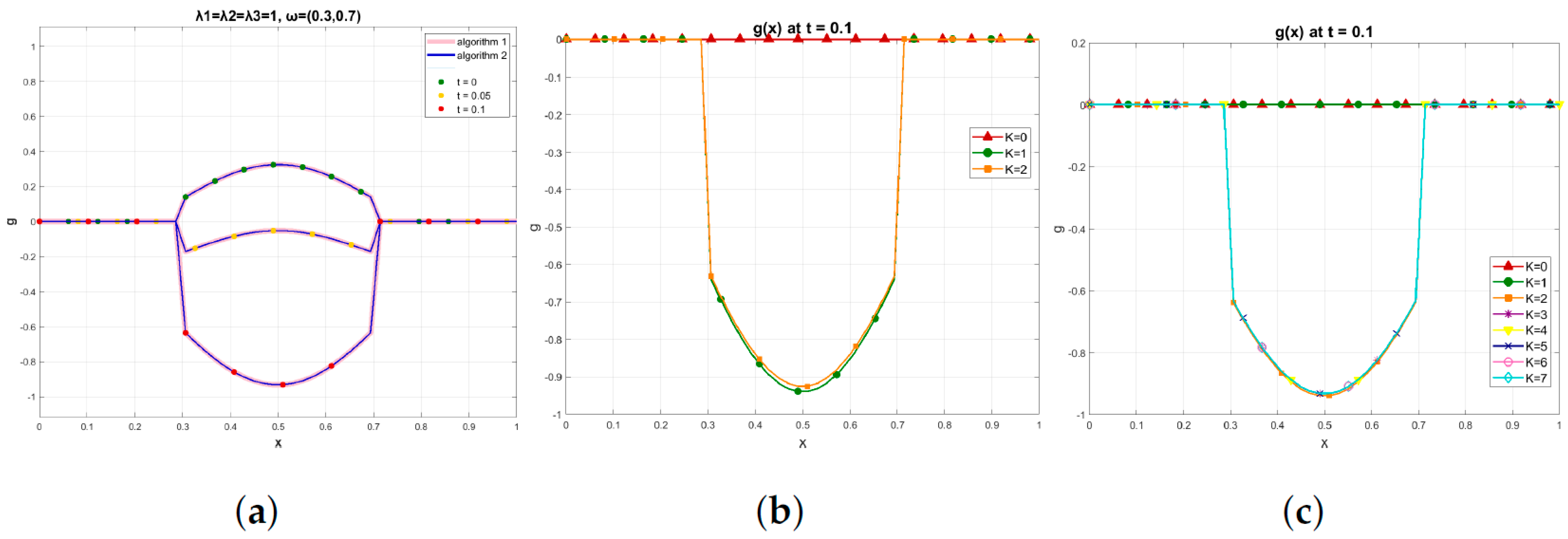
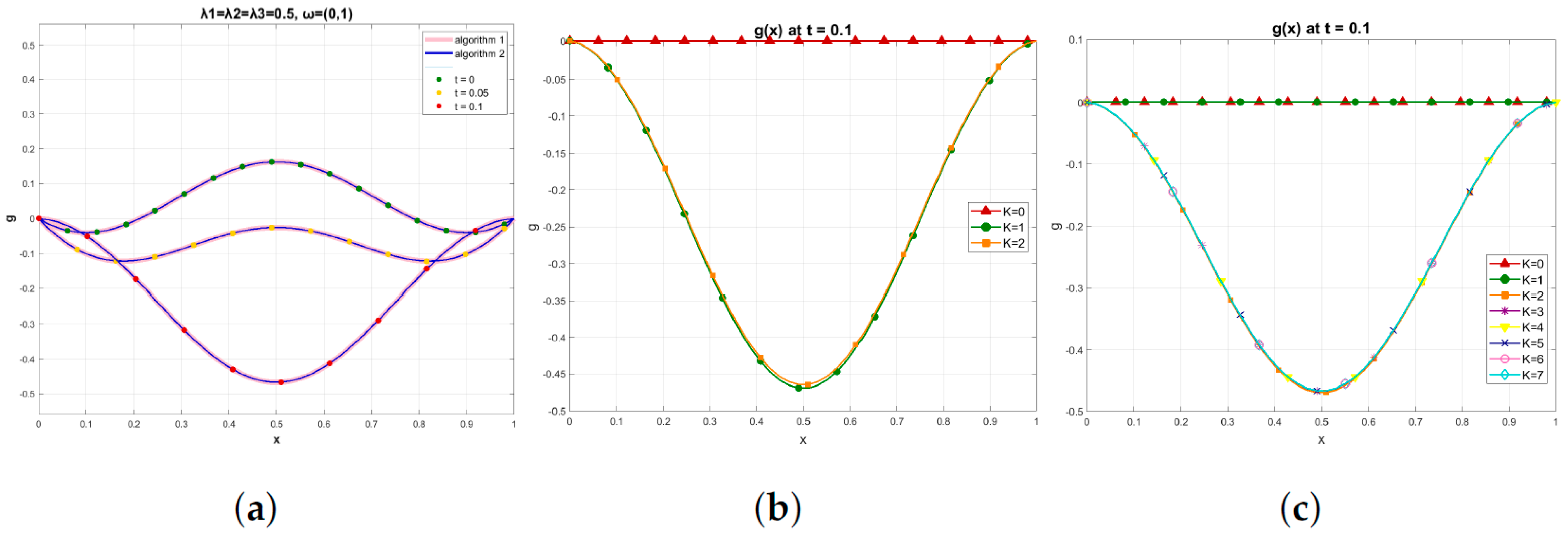
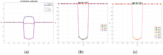
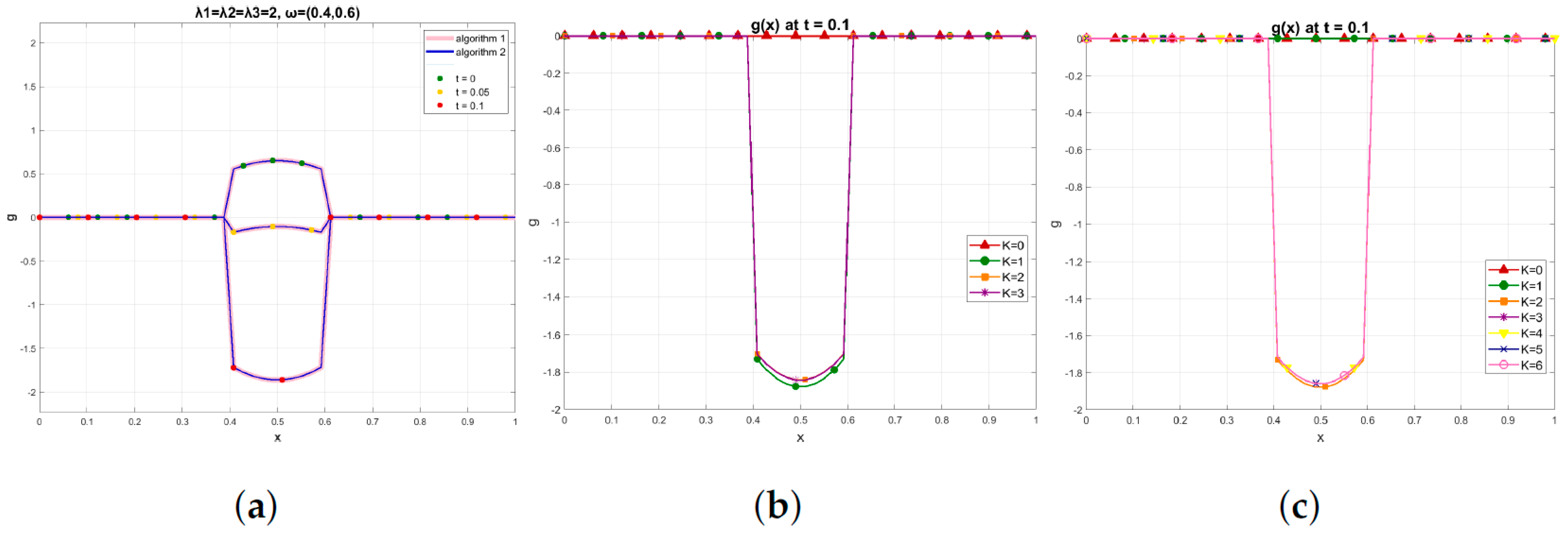
We performed all simulations in this section using MATLAB R2023a and present the results from Algorithms 1 and 2 in Figure 1, Figure 2 and Figure 3.

Figure 1. Comparison of Optimal Control with Two Methods for ${\lambda }_1={\lambda }_2={\lambda }_3=1,\omega =(0.3,0.7)$.

Figure 2. Comparison of Optimal Control with Two Methods for ${\lambda }_1={\lambda }_2={\lambda }_3=0.5,\omega =(0,1)$.

Figure 3. Comparison of Optimal Control with Two Methods for ${\lambda }_1={\lambda }_2={\lambda }_3=2,\omega =(0.4,0.6)$.

Figure 1a displays the optimal control computed by the two methods at $t=0,0.05,0.1$ with ${\lambda }_1={\lambda }_2={\lambda }_3=1,\omega =(0.3,0.7)$. Figure 1b shows the control function obtained with Algorithm 1 at $t=0.1$ during the K-th iteration ($K=0,1,2$). Figure 1c presents the corresponding control function obtained with Algorithm 2 during the K-th iteration ($K=0,1,2,\cdots$, 7).

Figure 2a displays the optimal control computed by the two methods at $t=0,0.05,0.1$ with ${\lambda }_1={\lambda }_2={\lambda }_3=0.5,\omega =(0,1)$. Figure 2b shows the control function obtained with Algorithm 1 at $t=0.1$ during the K-th iteration ($K=0,1,2$). Figure 2c presents the corresponding control function obtained with Algorithm 2 during the K-th iteration ($K=0,1,2,\cdots$, 7).

Figure 3a displays the optimal control computed by the two methods at $t=0,0.05,0.1$ with ${\lambda }_1={\lambda }_2={\lambda }_3=2,\omega =(0.4,0.6)$. Figure 3b shows the control function obtained with Algorithm 1 at $t=0.1$ during the K-th iteration ($K=0,1,2$). Figure 3c presents the corresponding control function obtained with Algorithm 2 during the K-th iteration ($K=0,1,2,\cdots$, 6).

As can be seen in Table 1, the minimum values of J obtained by Algorithms 1 and 2 are identical, yet Algorithm 1 requires fewer iterations.

Table 1. Comparison of Algorithms 1 and 2.

	${\mathit{\lambda }}_1={\mathit{\lambda }}_2={\mathit{\lambda }}_3=1,\mathit{\omega }=(0.3,0.7)$		${\mathit{\lambda }}_1={\mathit{\lambda }}_2={\mathit{\lambda }}_3=0.5,\mathit{\omega }=(0,1)$		${\mathit{\lambda }}_1={\mathit{\lambda }}_2={\mathit{\lambda }}_3=2,\mathit{\omega }=(0.4,0.6)$
	minJ (g)	Number of Iterations	$\mathit{minJ}$ (g)	Number of Iterations	$\mathit{minJ}$(g)	Number of Iterations
Algorithm 1	2.1816	2	1.0910	2	4.3627	3
Algorithm 2	2.1816	7	1.0910	7	4.3627	6

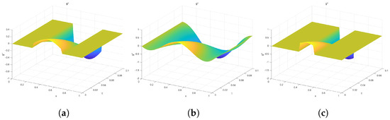
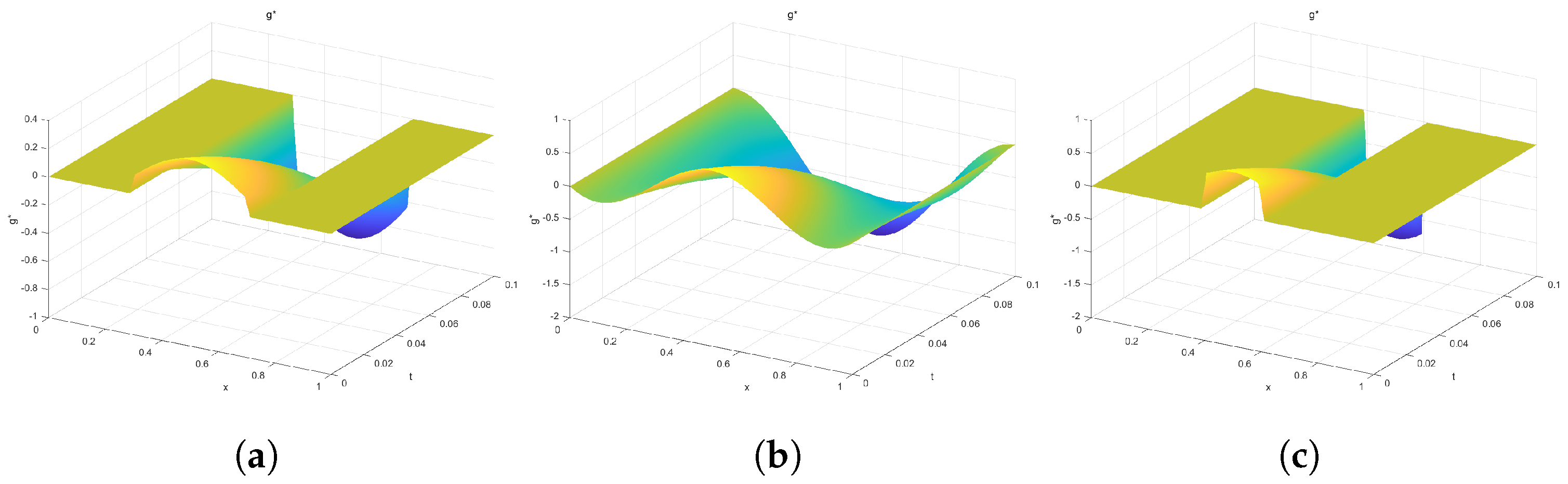
Figure 4a–c display the optimal control computed by Algorithm 1 with ${\lambda }_1={\lambda }_2={\lambda }_3=1,\omega =(0.3,0.7)$, ${\lambda }_1={\lambda }_2={\lambda }_3=0.5,\omega =(0,1)$, and ${\lambda }_1={\lambda }_2={\lambda }_3=2,\omega =(0.4,0.6)$, respectively.

Figure 4. Optimal Control via Algorithm 1 for Various Cases.

Below, Algorithm 1 is employed in order to analyze the physical interpretation of the numerical results.

Table 2 compares the objective functional J (and its constituent terms) between the uncontrolled case and the optimal control case with ${\lambda }_1={\lambda }_2={\lambda }_3$ and $\omega =(0.3,0.7)$. The application of optimal control leads to a reduction in J. Moreover, it decreases the terminal velocity $\parallel v(·,T)\parallel L^2(0,1)$ and temperature $\parallel \theta (·,T)\parallel L^2(0,1)$, but increases the terminal density ${\parallel \rho (·,T)\parallel }_{L^2(0,1)}$. The reduction in velocity is the most pronounced among these changes.

Table 2. Comparison between no control and optimal control.

g	$\mathit{minJ}$ (g)	${\parallel \mathit{g}\parallel }_{{\mathit{L}}^2(\mathit{\omega }\times (0,0.1))}$	${\parallel \mathit{\rho }(·,\mathit{T})\parallel }_{{\mathit{L}}^2(0,1)}$	${\parallel \mathit{v}(·,\mathit{T})\parallel }_{{\mathit{L}}^2(0,1)}$	${\parallel \mathit{\theta }(·,\mathit{T})\parallel }_{{\mathit{L}}^2(0,1)}$
0	2.1838	0	2.0073	0.5791	0.0534
$g^{*}$	2.1816	0.0661	2.0075	0.5710	0.0531

Table 3 illustrates the variation of the terminal $L^2$ norms with respect to the weighting parameters ${\lambda }_1,{\lambda }_2,{\lambda }_3$ and the control domain $\omega$. When ${\lambda }_2,{\lambda }_3,\omega$ are fixed, ${\parallel \rho (·,T)\parallel }_{L^2(0,1)}$ increases as ${\lambda }_1$ decreases and decreases as ${\lambda }_1$ increases. Similarly, for fixed ${\lambda }_1,{\lambda }_3,\omega$, ${\parallel v(·,T)\parallel }_{L^2(0,1)}$ increases with decreasing ${\lambda }_2$ and decreases with increasing ${\lambda }_2$. Under fixed ${\lambda }_1,{\lambda }_2,\omega$, ${\parallel \theta (·,T)\parallel }_{L^2(0,1)}$ remains unchanged, and each of the remaining terms in J changes only slightly. Finally, keeping ${\lambda }_1,{\lambda }_2,{\lambda }_3$ constant, the control effort $\parallel g^{*}{\parallel }_{L^2(\omega \times (0,T)}$ becomes larger when $\omega$ expands and smaller when $\omega$ contracts. Furthermore, the sensitivity analysis indicates that the objective functional J is most sensitive to variations in the weight ${\lambda }_1$. This implies that, among the terminal state terms in J, the density term ${\parallel \rho (·,T)\parallel }_{L^2(0,1)}$ exerts the dominant influence on the total cost.

Table 3. Comparison of different parameters and the locations of the control domain.

${\mathit{\lambda }}_1$	${\mathit{\lambda }}_2$	${\mathit{\lambda }}_3$	$\mathit{\omega }$	$\mathit{minJ}\left(\mathit{g}\right)$	$\parallel {\mathit{g}}^{*}{\parallel }_{{\mathit{L}}^2(\mathit{\omega }\times (0,0.1))}$	${\parallel \mathit{\rho }(·,\mathit{T})\parallel }_{{\mathit{L}}^2(0,1)}$	${\parallel \mathit{v}(·,\mathit{T})\parallel }_{{\mathit{L}}^2(0,1)}$	${\parallel \mathit{\theta }(·,\mathit{T})\parallel }_{{\mathit{L}}^2(0,1)}$
1	1	1	(0.3, 0.7)	2.1816	0.0661	2.0075	0.5710	0.0531
0.5	1	1	(0.3, 0.7)	1.1734	0.0759	2.0087	0.5664	0.0527
2	1	1	(0.3, 0.7)	4.1941	0.0955	2.0049	0.5801	0.0538
1	0.5	1	(0.3, 0.7)	2.0989	0.0480	2.0061	0.5797	0.0536
1	2	1	(0.3, 0.7)	2.3398	0.1485	2.0100	0.5545	0.0521
1	1	0.5	(0.3, 0.7)	2.1808	0.0662	2.0075	0.5710	0.0531
1	1	2	(0.3, 0.7)	2.1830	0.0659	2.0074	0.5711	0.0531
1	1	1	(0, 1)	2.1801	0.0846	2.0074	0.5661	0.0531
1	1	1	(0.4, 0.6)	2.1826	0.0493	2.0073	0.5749	0.0532

5. Conclusions

This paper has presented a theoretical analysis and a numerical example of the optimal control problem for the non-isentropic compressible Navier–Stokes equations linearized around a constant steady state in one dimension. Our main contributions include establishing foundational a priori estimates for the linearized state system, proving the existence and uniqueness of the optimal control, and deriving its explicit characterization through an optimality system, which was subsequently validated numerically. However, this study is limited to the case where the first variable of the constant steady state is zero. The more general scenario where this variable is non-zero has not been considered, as it necessitates the prescription of a boundary condition for the density. The well-posedness theory for weak solutions under such boundary conditions differs fundamentally from the case studied here and presents significant additional analytical challenges.

Furthermore, generalizing the results to more complex cases, such as multidimensional domains or systems linearized around non-constant or unstable steady states, raises considerable theoretical and practical challenges, including issues related to geometric complexity, enhanced coupling effects, and numerical stability. Investigating these more general cases, along with the aforementioned nonzero steady-state scenario, will therefore be an important objective for future research. Beyond this, further work will aim to extend the analysis to more complex and physically relevant compressible fluid flows, advancing the control theory in both theoretical and applied directions.

References

- Desai, M.; Ito, K. Optimal controls of Navier–Stokes equations. SIAM J. Control Optim. 1994, 32, 1428–1446. [Google Scholar] [CrossRef] [Scilit]
- Ghattas, O.; Bark, J.H. Optimal control of two- and three-dimensional incompressible Navier–Stokes flows. J. Comput. Phys. 1997, 136, 231–244. [Google Scholar] [CrossRef] [Scilit]
- Roubíček, T.; Tröltzsch, F. Lipschitz stability of optimal controls for the steady-state Navier–Stokes equations. Control Cybern. 2003, 32, 683–705. [Google Scholar]
- Wang, G. Pontryagin’s maximum principle for optimal control of the stationary Navier–Stokes equations. Nonlinear Anal. Theory Methods Appl. 2003, 52, 1853–1866. [Google Scholar] [CrossRef] [Scilit]
- De Los Reyes, J.C.; Tröltzsch, F. Optimal control of the stationary Navier–Stokes equations with mixed control-state constraints. SIAM J. Control Optim. 2007, 46, 604–629. [Google Scholar] [CrossRef] [Scilit]
- De Los Reyes, J.C.; Griesse, R. State-constrained optimal control of the three-dimensional stationary Navier–Stokes equations. J. Math. Anal. Appl. 2008, 343, 257–272. [Google Scholar] [CrossRef] [Scilit]
- Hintermüller, M.; Keil, T. Strong stationarity conditions for the optimal control of a Cahn-Hilliard-Navier–Stokes system. Appl. Math. Optim. 2024, 89, 12. [Google Scholar] [CrossRef] [Scilit]
- Casas, E.; Kunisch, K. First- and second-order optimality conditions for the control of infinite horizon Navier–Stokes equations. Optimization 2025, 74, 3037–3080. [Google Scholar] [CrossRef] [Scilit]
- López-Ríos, J.; Villamizar-Roa, É.J. An optimal control problem related to a 3D-chemotaxis-Navier–Stokes model. ESAIM Control Optim. Calc. Var. 2021, 27, 58. [Google Scholar] [CrossRef] [Scilit]
- Doboszczak, S.; Mohan, M.T.; Sritharan, S.S. Existence of optimal controls for compressible viscous flow. J. Math. Fluid Mech. 2018, 20, 199–211. [Google Scholar] [CrossRef] [Scilit]
- Chowdhury, S.; Ramaswamy, M. Optimal control of linearized compressible Navier–Stokes equations. ESAIM Control Optim. Calc. Var. 2013, 19, 587–615. [Google Scholar] [CrossRef] [Scilit]
- Doboszczak, S.; Mohan, M.T.; Sritharan, S.S. Pontryagin maximum principle for the optimal control of linearized compressible Navier–Stokes equations with state constraints. Evol. Equ. Control Theory 2022, 11, 347–371. [Google Scholar] [CrossRef] [Scilit]
- Ghezal, A.; Al Ghafli, A.A.; Al Salman, H.J. Anomalous Drug Transport in Biological Tissues: A Caputo fractional approach with non-classical boundary modeling. Fractal Fract. 2025, 9, 508. [Google Scholar] [CrossRef] [Scilit]
- Sunmitha, S.; Vivek, D.; Abdelfattah, W.M.; Elsayed, E.M. Advanced ILC analysis of switched systems subject to non-instantaneous impulses using composite fractional derivatives. AppliedMath 2025, 5, 115. [Google Scholar] [CrossRef] [Scilit]
- Maity, D. Some controllability results for linearized compressible Navier–Stokes system. ESAIM Control Optim. Calc. Var. 2015, 21, 1002–1028. [Google Scholar] [CrossRef] [Scilit]
- Chowdhury, S.; Ramaswamy, M.; Raymond, J.P. Controllability and stabilizability of the linearized compressible Navier–Stokes system in one dimension. SIAM J. Control Optim. 2012, 50, 2959–2987. [Google Scholar] [CrossRef] [Scilit]
- Stojanovic, S. Optimal damping control and nonlinear elliptic systems. SIAM J. Control Optim. 1991, 29, 594–608. [Google Scholar] [CrossRef] [Scilit]
Disclaimer/Publisher’s Note: The statements, opinions and data contained in all publications are solely those of the individual author(s) and contributor(s) and not of MDPI and/or the editor(s). MDPI and/or the editor(s) disclaim responsibility for any injury to people or property resulting from any ideas, methods, instructions or products referred to in the content. |
© 2026 by the authors. Licensee MDPI, Basel, Switzerland. This article is an open access article distributed under the terms and conditions of the Creative Commons Attribution (CC BY) license.