


Abstract
In autonomous manufacturing systems, the performance of time-series-based anomaly detection and fault diagnosis is highly sensitive to window size selection. Conventional approaches rely on empirical rules or fixed window settings, which often fail to capture the diverse temporal characteristics of anomalies and lead to performance degradation. This study systematically addresses the window size selection problem by categorizing anomaly patterns into three representative types: variability, cycle, and local spike. Each pattern is associated with a distinct temporal scale and underlying physical mechanism. Based on this insight, an Anomaly Deviation-Based Window Size Selection (ADW) method is proposed, which quantitatively evaluates anomaly deviation as a function of window size. Unlike traditional preprocessing-oriented approaches, the proposed method redefines window size as a core design variable that directly governs anomaly representation and diagnostic sensitivity. The effectiveness of the ADW method is validated using tension data from a roll-to-roll continuous manufacturing process and vibration data from a rotating bearing fault dataset. Experimental results demonstrate that the proposed approach consistently identifies optimized window sizes tailored to different anomaly types, leading to improved fault classification accuracy and diagnostic robustness. The proposed framework provides a physically interpretable and data-driven guideline for adaptive window size selection in long-term autonomous manufacturing systems.
Keywords:
window size selection; anomaly deviation; fault diagnosis; feature extraction; autonomous manufacturing MSC:
68T01
1. Introduction
Smart manufacturing industries are rapidly advancing toward higher production speeds, larger processing areas, and greater precision. Accordingly, the importance of process condition monitoring technologies for ensuring stable operation and quality reliability of manufacturing equipment continues to increase. Abnormal equipment behavior or process instability occurring during manufacturing directly leads to increased system downtime, higher defect rates, and increased maintenance costs. In particular, systems operating based on rotating machinery—such as wind turbines [1,2,3,4], aircraft engines [5,6,7,8,9,10], and roll-to-roll (R2R) production lines [11,12,13,14]—are highly susceptible to mechanical faults that can significantly degrade operational stability. For example, tension disturbances caused by roll eccentricity or bearing faults in R2R systems can propagate throughout the entire process, resulting in unstable operation and yield loss [15,16].
To proactively prevent such issues, anomaly detection and fault diagnosis techniques based on process data play a critical role. Multivariate time-series process data continuously acquired from sensors provide highly sensitive information reflecting changes in equipment conditions and early signs of abnormalities, thereby governing the efficiency and reliability of smart manufacturing systems. Recently, in the field of Fault Diagnosis and Classification (FDC), data-driven approaches that systematically construct process data through signal processing and domain-knowledge-based feature engineering, combined with feature selection and model lightweighting, have been rapidly expanding [17,18,19,20,21,22,23,24,25]. These approaches focus on achieving efficient learning and robust generalization performance under practical constraints, such as label scarcity and hardware limitations associated with large-scale data processing. In parallel, integrated frameworks that combine equipment condition monitoring and Remaining Useful Life (RUL) estimation using multivariate sensor streams, as well as lightweight models that explicitly consider data drift and data imbalance, have been actively reported, demonstrating tangible improvements in system lifetime extension and downtime reduction [26,27,28,29]. Such data-driven approaches have become a key driving force behind smart manufacturing, with anomaly detection and fault diagnosis established as core functions governing productivity and operational efficiency in production lines.
In time-series-based anomaly detection, most signal processing and learning methods assume window-based processing, in which data are segmented into fixed-length intervals [30,31,32,33,34,35,36]. In this context, defining the window size is an essential step to transform continuous time-series data into units suitable for feature extraction, serving as the foundation for subsequent dimensionality reduction and feature extraction processes [37]. The window size (W), which determines how the data are segmented, has a decisive impact on anomaly detection performance and influences the entire pipeline, including feature extraction, feature selection, and classification stages. Moreover, the window size directly affects computational latency and system stability. It determines the temporal range over which anomaly patterns are captured within a single feature representation, and is therefore closely related to anomaly reproducibility, feature stability, and final detection performance.
In conventional studies and practical industrial applications, window size is commonly determined based on a dominant period (T0) estimated via FFT or autocorrelation analysis (W ≈ 3–10·T0), or selected as a fixed value after performing grid search over a small set of empirically defined candidates [38,39,40]. Although such approaches are simple to implement, they fail to explicitly account for the characteristics and density of anomaly patterns appearing across multiple temporal scales. When the window size is excessively small, transient noise or local fluctuations are overly reflected in the extracted features, causing anomaly detection models to overfit abnormal patterns. This overfitting leads to frequent false alarms even under normal operating conditions, thereby degrading process stability and reliability. Conversely, when the window size is excessively large, the distinctive anomaly characteristics of normal and faulty classes are diluted through temporal averaging, resulting in reduced feature discriminability and potential failure to detect actual faults [41,42,43].
These observations indicate the existence of an inherent trade-off between overfitting and feature information loss in window size selection. Window size is not merely a parameter for segmenting data, but a critical variable that fundamentally alters the structure of the feature space learned by anomaly detection models by determining the temporal scope and density of information represented along the time axis. In other words, selecting a window size can be interpreted as deciding which temporal features to preserve and which to discard. This choice has a significant impact on feature selection within the learning framework [44,45,46,47]. Despite its critical role in determining the performance of anomaly detection pipelines, window size has not been sufficiently analyzed or mathematically formalized in prior studies. In particular, smart manufacturing process data often contain heterogeneous anomaly patterns with different temporal scales and densities, including short-term irregular signals, mid-term variability changes, and long-term variations in periodic structures. Such diversity in anomaly patterns is difficult to adequately capture using a single criterion or a fixed window size.
To address this limitation, this study quantitatively incorporates the temporal scales and densities of anomaly patterns in process data and mathematically analyzes the effects of window size on feature separability and anomaly reproducibility. Based on this analysis, a window size selection method is proposed. The proposed approach defines window size not as an empirical parameter, but as an optimization variable that maximizes feature separability between normal and faulty data, thereby formulating the window size selection problem in a mathematical framework. This formulation enables systematic modeling of the trade-off between overfitting and information loss, allowing the derivation of a window size optimized for anomaly detection objectives. The proposed method is applied to datasets containing diverse cycle–variability–irregularity patterns as well as real multivariate sensor streams, and its superiority over conventional fixed or empirical window settings is validated in terms of anomaly detection performance and stability. Furthermore, experiments conducted on roll-to-roll continuous process data with mechanical disturbances and bearing fault datasets demonstrate the applicability of the proposed method. The experimental results confirm that optimizing the window size leads to a significant improvement in anomaly detection performance while effectively suppressing overfitting.
The ultimate goal of this study is to provide a practical window size selection procedure applicable to smart manufacturing pipelines, thereby offering an effective approach for improving fault diagnosis and predictive maintenance performance under real-world constraints such as data imbalance and data drift.
The main contributions of this paper are summarized as follows:
- A mathematical analysis of the effects of window size on feature separability and anomaly reproducibility is presented by quantitatively reflecting the temporal scales and densities of anomaly patterns in process data, and a corresponding window size selection method is proposed.
- The proposed method is applied to datasets containing diverse cycle–variability–irregularity patterns and real multivariate sensor streams, enabling improved anomaly detection performance and stable feature selection compared to conventional fixed or empirical window settings.
- A window size selection procedure applicable to smart manufacturing pipelines is presented, providing a practical solution for enhancing fault diagnosis and predictive maintenance performance while considering real-world constraints such as data imbalance and data drift.
2. Theoretical Background
2.1. Problem Definition
As maintenance methodologies have recently shifted toward data-driven approaches, fault diagnosis and prognostic performance based on machine learning and deep learning techniques has continuously improved (Figure 1) [48]. The performance of such data-driven fault diagnosis algorithms strongly depends on how effectively informative features are extracted and selected from the input data. In particular, for time-series process data, the appropriate selection of window size during the preprocessing stage for feature selection is a critical data processing step that determines both feature quality and learning efficiency [49].
Figure 1.
Fault Diagnosis and Classification Flowchart with Window Size Selection. The layered green boxes indicate that the model training and validation processes are iteratively conducted across multiple candidate window sizes and dataset conditions.
In time-series-based anomaly detection, the window size defines the temporal range over which raw sensor signals are aggregated into a single feature representation, thereby directly governing the information density and discriminative power of the extracted features. When the window size is excessively small, features become overly sensitive to transient anomalies or sensor noise, causing the model to overfit to local fluctuations. Conversely, as the window size increases, statistical stability improves; however, class-discriminative characteristics that distinguish normal and faulty states are diluted through temporal averaging, resulting in degraded feature separability [50].
This phenomenon indicates the existence of an inherent trade-off between overfitting and the loss of class-discriminative information depending on the window size (Figure 2). Nevertheless, in most existing studies and industrial practices, window size has been determined primarily based on heuristic criteria or empirical rules, which limits the ability to sufficiently reflect the characteristics of anomaly patterns inherent in the data. To address this limitation, this study defines the trade-off as a function of feature separability between normal and faulty data and mathematically formulates the window size selection problem as a feature selection problem along the time axis by identifying the window size that maximizes this separability.
Figure 2.
Trade-off between overfitting and class-discriminative information loss as a function of window size. The structure of the processed data varies with the selected window size, and classification accuracy improves when an optimal window size is chosen.
2.2. Distinction from Existing Multi-Scale and Deep Learning Approaches
Recent studies on fault diagnosis in manufacturing systems have increasingly focused on multi-scale deep learning architectures, including CNN-based hierarchical models, hybrid CNN–LSTM frameworks, and more recently, hybrid Mamba–CNN architectures [51,52]. These approaches aim to enhance diagnostic performance by learning temporal representations at multiple resolutions through architectural design, enabling the model to capture both short-term fluctuations and long-term dependencies. Despite their effectiveness, such methods primarily address the problem at the model level, assuming that the underlying window-based data representation is given or empirically determined. In most existing studies, window size is selected heuristically, fixed across experiments, or optimized indirectly through model-specific validation. As a result, the influence of window size itself on feature separability, anomaly visibility, and learning stability is often overlooked or implicitly absorbed into model complexity.
In contrast, the present study addresses a fundamentally different and complementary problem: principled window size selection at the data representation level prior to model training. Rather than proposing a new network architecture or multi-scale learning mechanism, this work focuses on quantitatively analyzing how window size interacts with the temporal characteristics and density of anomaly patterns. The proposed anomaly deviation-based formulation explicitly evaluates the effect of window size on different anomaly mechanisms, independent of any specific learning model.
From this perspective, the proposed method is model-agnostic and orthogonal to existing multi-scale deep learning approaches. It does not compete with advanced architectures such as hybrid Mamba–CNN models but instead provides a systematic preprocessing strategy that can be directly combined with them. Specifically, the proposed method can guide the selection of a base window size or inform the design of scale ranges in multi-scale frameworks, thereby improving the quality of input representations before any model-level optimization is performed. By clearly separating the roles of data representation and model architecture, this study contributes a missing methodological component to existing fault diagnosis pipelines. The proposed approach complements, rather than replaces, multi-scale deep learning methods and offers a generalizable solution for window size determination that remains effective across diverse modeling choices and operating conditions.
2.3. Time Series Data and Window Size
This section briefly describes the theoretical background for the proposed window size selection method [31]. Sensor data acquired from smart manufacturing processes are assumed to be a d-dimensional multivariate time series, denoted as for . Here, represents a discrete time index with a uniform sampling interval , where denotes the sampling frequency. For anomaly detection and feature extraction, the entire time series is segmented into subsequences of length . The -th windowed subsequence of length is defined as Equation (1).
Here, denotes the hop size, which represents the shift interval between adjacent windows, and the window overlap ratio is defined as Equation (2) [53,54]. For univariate sensor data, can be simplified to a scalar . Such a sliding window model is standardly employed not only for extracting simple statistical features, such as mean, variance, and kurtosis, but also for time–frequency analyses based on the Fast Fourier Transform (FFT) and Short-Time Fourier Transform (STFT).
Under this framework, the time and frequency resolutions are determined by the window size and hop size as and , respectively. In general, increasing improves frequency resolution while degrading time resolution. Conversely, decreasing enhances the ability to capture transient variations but makes it more difficult to separate adjacent frequency components, resulting in a fundamental trade-off between time and frequency resolution. Owing to these characteristics, the window size is regarded as a critical hyperparameter in a wide range of time-series-based data mining tasks, including anomaly detection and classification for fault diagnosis. In particular, prior studies have reported that inappropriate window size selection can significantly degrade overall diagnostic performance by reducing feature separability, diluting anomaly patterns, or excessively increasing sensitivity to noise.
2.4. Anomaly Pattern Based on Window Size
Window size directly affects not only the time and frequency resolution but also the visibility of anomaly patterns inherent in time-series data. Since different types of anomaly patterns require different temporal scales for reliable characterization, the window size should be selected to appropriately reflect the characteristics of each pattern.
First, for cycle-type anomaly patterns, a single window must contain at least multiple repetitions of the dominant period to stably capture the repetitive structure. Pai and Zhong applied Discrete Fourier Transform (DFT) and Short-Time Fourier Transform (STFT)-based techniques to vibration signal analysis in mechanical systems [55,56]. They demonstrated that a data length covering at least three to six cycles is required to reliably estimate the fundamental frequency and amplitude, and that the frequency estimation error decreases as the number of included cycles increases. These findings suggest that, for general cycle anomaly patterns, setting the window size on the order of Equation (3) enables stable observation of frequency peak locations and amplitude variations in the FFT domain. Such an approach constitutes a heuristic window size selection strategy that has been empirically validated in prior studies.
Conversely, when is excessively short, the number of cycles contained within a single window decreases to fewer than one or two, causing spectral peaks to spread or become unstable in the frequency domain. As a result, it becomes difficult to quantitatively characterize cycle-type anomalies, such as variations in periodicity or changes in peak amplitude.
Variability-type anomaly patterns represent long-term changes in the mean level or slope of a signal and can be expressed in terms of variations in the window-wise mean value [57,58]. When the window size is excessively small relative to the time scale of variability variation , each window captures only a nearly constant or locally linear segment. Consequently, variability changes manifest as very small differences in window-wise means, making them difficult to distinguish from noise. In contrast, when , different variability segments are mixed within a single window, leading to averaging effects that dilute the characteristics of variability anomalies. Therefore, to effectively reveal variability-type anomaly patterns, should be set to be comparable to or slightly larger than , and the region where the variance or standard deviation of window-wise means is maximized should be selected.
Local spike anomalies often appear as high-amplitude impacts confined to short time intervals, reflecting intermittent disturbances or impulsive faults. Such impulsive anomalies can be effectively quantified using higher-order statistics, such as kurtosis and spectral kurtosis (SK). Kurtosis measures the tail heaviness of a distribution, with larger values indicating stronger localized spikes. Antoni demonstrated that spectral kurtosis is highly sensitive to the presence and frequency location of transient components in nonstationary signals, and Wang et al. systematically showed through various case studies that spectral kurtosis serves as a powerful indicator for detecting the presence of impulsive faults and identifying energy-concentrated frequency bands in rotating machinery fault diagnosis [59,60]. These results imply that as the window size increases, the relative contribution of short-duration local spike anomalies within a window decreases, causing the spike-induced increase in kurtosis to be averaged out. Consequently, the difference in kurtosis between windows containing spikes and those without spikes is reduced. Conversely, when is excessively small, windows with accidentally high kurtosis due to noise or minor fluctuations increase, making it difficult to distinguish true spike-type anomalies from false alarms.
As discussed above, cycle, variability, and local spike anomalies are characterized by distinct temporal scales—namely the period , the variability variation time , and the spike duration , respectively. The window size, depending on its relative magnitude with respect to these scales, simultaneously determines the reproducibility, visibility, and detection delay of anomaly patterns. Recent studies on window size selection have also reported that inappropriate window sizes significantly degrade the performance not only of anomaly detection but also of various unsupervised time-series analysis tasks, such as time-series segmentation and motif discovery. These studies emphasize the necessity of window design that explicitly reflects temporal characteristics, including anomaly periodicity and duration [56,61]. Accordingly, this study aims to design the window size by quantitatively incorporating the temporal scales and densities of anomaly patterns inherent in manufacturing process data.
3. Methodology
3.1. Procedural Flowchart of the Anomaly Deviation-Based Window Size Selection
As illustrated in Figure 3, the proposed Anomaly Deviation-Based Window Size Selection (ADW) process consists of a total of eight steps. These steps can be broadly categorized into three main stages. The first stage involves data acquisition and labeling. The second stage focuses on defining and analyzing anomaly patterns within time-series data to derive deviation scores. The third stage consists of window size determination and validation.
Figure 3.
Flowchart of Anomaly Deviation-Based Window Size Selection (ADW) Methodology.
Step 1: Raw time-series data are collected from sensors installed in the manufacturing equipment.
Step 2: In this step, the acquired raw data are classified into normal and faulty datasets. In this study, normal and fault conditions are categorized on a case-by-case basis for each dataset to validate the proposed window size selection method.
Step 3: Anomaly patterns are defined for each labeled dataset. As described earlier, three types of anomaly patterns are considered in this study: variability, cycle, and local spike.
Steps 4–6: Deviation scores, which serve as indicators for evaluating the anomaly severity within the data, are derived by considering the defined anomaly patterns. Statistical feature variables are utilized to assess anomaly levels, and normal and faulty data are distinguished through the computation and comparison of deviation scores. Detailed descriptions of the deviation score formulation are provided in Section 3.2.
Step 7: In this step, the window size is calculated based on the deviation scores obtained in Steps 4–6 and the sampling rate. The window size derived by explicitly considering anomaly characteristics contributes to improving the temporal and computational efficiency of the subsequent learning model.
Step 8: The derived window size is validated in this stage. Since the window size determines the range of data patterns learned by the model, inappropriate selection may lead to model overfitting. In this step, the validity of the derived window size is assessed by evaluating precision, F1-score during model training, thereby verifying whether the selected window size effectively mitigates overfitting and is appropriate for anomaly detection.
3.2. Proposed Method: Anomaly Deviation-Based Window Size Selection
In this study, anomaly patterns are quantitatively characterized based on statistical variables by considering three commonly identified anomaly types: variability, cycle, and local spike.
3.2.1. ADW Method Overview
The proposed window size selection method is conducted through the following procedure:
- (1)
- The dominant period is estimated from raw time-series data acquired from process sensors, and an analysis period is defined accordingly.
- (2)
- Based on the analysis period, variability, cycle, and local spike anomaly patterns are quantified using statistical features for a range of candidate window sizes .
- (3)
- The deviations between normal and faulty cases are compared for each window size, and the window size that most consistently and balancedly reveals the three anomaly patterns is selected.
In other words, the window size is treated not as a user-dependent hyperparameter but as a design variable that reflects the temporal scales of variability, cycle, and local spike anomaly patterns. From this perspective, the optimal window size is determined in a data-driven manner.
3.2.2. Analysis Period and Candidate Window Size Definition
Given multivariate raw time-series data collected from process sensors, the dominant frequency is estimated by performing a Fast Fourier Transform (FFT) over a sufficiently long observation interval. The estimated dominant frequency is then converted into the dominant period in the time domain as . This dominant period is used as a reference for defining the search range of the window size.
To stably capture cycle-type anomalies, the window size search range is defined as in Equation (4). The lower bound is set to include at least three cycles, while the upper bound is determined by considering detection delay and computational complexity.
However, the proposed method does not restrict the search to discrete multiples of the dominant period. Instead, multiple candidate window lengths are evaluated within the range to identify a window size that can simultaneously capture the information of the three anomaly patterns within a single window. The set of candidate window sizes () is defined as Equation (5).
Here, denotes the search resolution. When , anomaly patterns are evaluated for all window sizes from to . When , only window sizes sampled at fixed intervals are evaluated. For each , overlapping windows are constructed using a hop size defined as .
3.2.3. Statistical Features by Pattern and Definition of Deviation
For each candidate window size , the normal dataset and the faulty dataset are segmented into windowed subsequences using the same window size () and hop size (), where . Here, denotes the window index, and represents the normal or faulty condition. For each window size, the following three statistical features are computed simultaneously to quantitatively characterize variability, local spike, and cycle anomaly patterns. Their conceptual meanings are illustrated in Figure 4. Variability anomalies correspond to gradual changes in the mean signal level, local spike anomalies represent aperiodic and sporadically occurring irregular outlier points, and cycle anomalies refer to changes in the dominant periodicity of the signal.
Figure 4.
Schematic illustration of three anomaly types: variability, local spike and cycle. The blue-shaded regions denote intervals exhibiting significant numerical variations characteristic of each anomaly type.
Window size determines not only the level of information aggregation within a single window but also the variability of features across consecutive windows. As the window size decreases, sensitivity to noise and local fluctuations increases, leading to higher feature variability, whereas increasing the window size reduces variability due to temporal averaging effects. The standard deviation directly measures this window-to-window variability and exhibits continuous and monotonic behavior with respect to changes in window size. Therefore, it effectively captures the trade-off between noise sensitivity and temporal averaging, and the three anomaly indicators are defined based on the standard deviation in this study. In addition, although Variability, Cycle, and Local spike anomalies are quantified using different statistical features, they share a common structure in that all features are computed as window-wise scalar values. By adopting the standard deviation as a common dispersion operator, a consistent deviation definition can be established across heterogeneous anomaly indicators, enabling the visibility of anomalies with respect to window size to be compared and integrated within a unified interpretative framework.
A variability anomaly refers to a pattern in which the signal mean varies gradually over time and is quantified through the variability of window-wise means. The mean of the k-th window for condition(c) is defined in Equation (6). The variability index at a given window size is defined as the standard deviation of the window-wise means, as shown in Equation (7). This index represents the extent to which the window-wise means vary across time segments, regardless of whether the values increase or decrease. The deviation of variability anomalies between normal and faulty conditions is defined in Equation (8). A larger value indicates better separability between normal and faulty data from the perspective of variability patterns. Here, Variability denotes the variation in window-wise means quantified by their standard deviation, and it does not represent the direction (increasing/decreasing) of change.
A local spike anomaly manifests as a localized irregular pattern, such as a short-duration, high-amplitude impact, and is quantified through the variability of window-wise kurtosis. The kurtosis of the -th window for condition is defined as in Equation (9). The spike index at a given window size is defined as the standard deviation of the window-wise kurtosis, as shown in Equation (10). This index reflects the degree of variability associated with the occurrence and location of localized spikes.
The deviation of spike anomalies between normal and faulty conditions is defined as in Equation (11). A larger value of indicates higher separability between the two groups from the perspective of spike anomaly patterns.
A cycle anomaly refers to a pattern in which the magnitude or stability of the dominant frequency component changes and is quantified through the variability of window-wise FFT peaks. For each window, an FFT is performed, and the maximum amplitude within the frequency band of interest around the dominant frequency is defined as in Equation (12). The cycle index is defined as the standard deviation of the window-wise FFT peak amplitudes, as shown in Equation (13), representing the degree to which the strength of the periodic component varies over time. The deviation of cycle anomalies between normal and faulty conditions is defined as in Equation (14).
As a result, for each window length , a three-dimensional deviation vector defined in Equation (15) is obtained. This vector quantitatively summarizes how well the normal and faulty data are separated at the given window length from the perspectives of variability, local spike, and cycle anomaly patterns
3.2.4. Interpretation of the Integrated Deviation Score
The three deviation measures defined above—, , and —are designed to reflect different anomaly mechanisms. Accordingly, the physical quantities and computational formulations used to define each deviation differ, as described in Equations (16)–(18). Variability deviation is defined based on structural changes in low-frequency components, such as variations in window-wise means or slopes. In contrast, local spike deviation is defined using higher-order statistics, such as kurtosis or spectral kurtosis, which are sensitive to transient high-amplitude events. Cycle deviation is based on frequency-domain characteristics, including the dominant period and changes in spectral peak location, amplitude, and band energy.
As a result, each deviation measure exhibits different numerical scales, distribution characteristics, dynamic ranges, and units. Therefore, for a given window size, directly comparing their magnitudes or simply summing them is not statistically meaningful. In particular, , which is defined based on kurtosis, tends to exhibit heavy-tailed distributions, leading to extreme values in certain windows. In such cases, an integrated metric may become excessively dominated by a specific anomaly type.
For these reasons, this study normalizes each pattern-specific deviation into a relative score within the range , as defined in Equations (16)–(18), to enable fair comparison across window sizes and balanced integration among different anomaly types. The objective of this study is not to maximize the detection performance of a specific anomaly type, but to derive a window size that mitigates the trade-off between underfitting and overfitting and ensures stable generalization performance. To this end, prior bias toward any particular anomaly type is deliberately avoided, and anomaly patterns with different time scales and physical mechanisms are incorporated in a balanced manner. Based on this design principle, equal weights are assigned to the deviation scores of all anomaly types in Equation (19) to construct the integrated deviation score.
For the candidate window size set , the normalized deviation for each anomaly pattern is defined to represent relative performance within the candidate set. A value of indicates that the window size provides the maximum separability among all candidates from the perspective of the corresponding anomaly pattern, whereas indicates the weakest performance. Through this normalization, deviations with different physical meanings are mapped onto a common interpretative axis of “relative superiority within the candidate set,” thereby providing a directly comparable metric suitable for window size selection.
The three normalized deviations are integrated in the form of a weighted sum to construct an integrated deviation score for each window size. The score is interpreted as a scalar indicator that summarizes the relative visibility and separability provided by a given window size across multiple anomaly patterns. The optimal window size is then selected as the value that maximizes . The weighted-sum formulation enables the trade-offs among anomaly patterns with different temporal scales and physical characteristics to be coordinated within a single objective function, and the weights can be adjusted according to domain requirements or the relative importance of specific fault types.
In Equation (19), equal weights are assigned to the normalized deviation scores corresponding to variability, cycle, and local spike anomaly patterns. This design choice is motivated by the objective of this study, which is not to optimize detection performance for a specific anomaly type, but to derive a window size that ensures robust and stable generalization performance across heterogeneous anomaly mechanisms commonly observed in manufacturing systems. From a practical perspective, manufacturing process data often contain multiple anomaly patterns simultaneously, and their relative importance is typically unknown a priori. Assigning unequal weights would implicitly introduce prior bias toward a specific anomaly type, potentially leading to a window size that overemphasizes certain temporal characteristics while suppressing others. Such bias may improve performance for a particular fault scenario but can degrade robustness under changing operating conditions or fault modes. By adopting equal weights, the proposed framework treats variability, cycle, and local spike deviations as equally important contributors to anomaly visibility, thereby enabling a balanced trade-off between underfitting and overfitting across multiple temporal scales [62,63]. This choice ensures that the selected window size does not overly favor short-term impulsive events or long-term periodic structures but instead maximizes overall feature separability in a general and model-agnostic manner. It is worth noting that the proposed formulation is not restricted to equal weights. In applications where domain knowledge or prior fault statistics are available, the weight vector can be adaptively adjusted to emphasize specific anomaly types. However, to maintain general applicability and avoid heuristic bias, equal weighting is adopted as the default configuration in this study.
The rationale for favoring larger deviation values can be interpreted for each anomaly type as follows, and these relationships are conceptually illustrated in Figure 5. A large variability deviation indicates that features based on window-wise means or slopes vary sufficiently over time, and that these variations reflect structural shifts induced by variability changes rather than random noise. When the window size is excessively small relative to the characteristic time of variability variation, each window captures only a nearly constant local segment, causing differences in window-wise means to remain at the noise level. In contrast, with an appropriate window size, window-wise means or slopes systematically shift across variability transition regions, increasing feature separability between normal and anomalous segments. This enhances sensitivity to variability-based anomalies while suppressing spurious false alarms caused by incidental mean fluctuations.
Figure 5.
Anomaly separability mechanism for variability, cycle, and local spike patterns. As the deviation score increases, the separability between normal and faulty data is enhanced, enabling the use of a larger window size and a lower resolution setting.
A large local spike deviation implies that higher-order statistics, such as kurtosis or spectral kurtosis, respond selectively and strongly in windows containing impulsive anomalies, clearly distinguishing them from windows without spikes. When the window size is excessively large, the proportion of spike anomalies within a window decreases, and the spike-induced increase in higher-order statistics is averaged out, thereby diluting feature differences between spike-containing and spike-free windows. Conversely, when the window size is excessively small, high kurtosis values may arise even from minor noise fluctuations, making it difficult to distinguish true impulsive faults from false spikes. Therefore, a window size yielding a large irregular deviation corresponds to a regime in which statistical measures respond sensitively only in the presence of spikes while remaining stable under normal conditions, thereby improving both detection performance and reliability for impulsive faults.
A large cycle deviation indicates that changes in periodic structure are stably and consistently reproduced on a window-by-window basis. If the window size is insufficiently large, the number of cycles contained within a window is inadequate, leading to unstable FFT- or STFT-based spectral peak estimation and inconsistent spectral differences between normal and anomalous conditions. In contrast, with an appropriate window size, a sufficient number of cycles are included, allowing spectral peak locations and amplitudes to be formed stably, and frequency shifts or amplitude changes to be clearly revealed in response to anomaly events. This improves feature reproducibility for cycle-type anomalies and effectively enhances separability between normal and faulty conditions in vibration-based fault diagnosis.
In summary, the three deviations quantify the visibility of anomaly patterns characterized by different temporal scales and physical mechanisms. The integrated deviation score, defined as the normalized weighted sum of these deviations, provides a window size selection criterion that balances multiple anomaly patterns without bias toward a specific type. This approach redefines the window not as a simple preprocessing parameter but as a key design variable that governs anomaly deviation, enabling stable and reproducible window size determination even in complex manufacturing process data where variability changes, periodic variations, and impulsive events coexist.
3.2.5. Optimal Window Size Selection Based on Deviation Score
After computing the integrated deviation score for each candidate window size in the predefined set, we identify the candidate that yields the highest deviation score, which indicates the largest separability between normal and faulty data under the integrated deviation analysis. Equation (20) is then applied only after this maximum-score point is obtained, in order to express the corresponding window length in samples using the ratio between the sampling frequency and operating frequency. Therefore, Equation (20) should be understood as a post-processing conversion step, rather than a formula that performs the maximization or search by itself.
Equation (20) is applied after identifying the maximum deviation score point among candidate windows; it converts the corresponding window length into a sample-based representation and does not perform the maximization itself. Here, denotes the floor operator, which ensures an integer-valued window length. This formulation sets a baseline range for the window size such that a minimum amount of periodic information is included based on the physical operating cycle of the equipment, and subsequently adjusts the window length toward regions with high anomaly visibility using the deviation score. Specifically, when anomaly-induced deviations are observed to be large, a longer window is selected to stably capture structural changes, whereas when deviations are relatively small, a shorter window is chosen to emphasize localized variations. Through this mechanism, the proposed approach automatically determines a physically meaningful window size by jointly considering the sampling conditions and the operating characteristics of the equipment. Through this formulation, the deviation-score-based window size selection is established.
4. Validation Scenarios and Comparative Analysis
4.1. Experiment Setup
To validate the proposed window size design for feature selection, roll-to-roll (R2R) tension data and bearing vibration data were used.
4.1.1. Dataset 1: Tension Data
The Roll to Roll (R2R) system used in this study is designed to continuously process a flexible substrate under controlled tension. The system consists of an unwinder, a driven roll, and a rewinder, with multiple idle rolls used to transport the web. Such systems are widely employed in advanced manufacturing fields, including flexible electronics, printed sensors, and functional coatings, where precise tension control is essential to ensure product quality and process stability.
The tension data were acquired using a DACELL RTB15-K20 load cell installed at the infeeder section of the R2R slot-die coating system at the Continuous Process Center of Konkuk University, as illustrated in Figure 6a. The tension dataset is categorized into three operating conditions: (i) normal operation, (ii) infeeder roll eccentricity with one eccentric element, and (iii) infeeder roll eccentricity with two eccentric elements. These conditions were selected to evaluate the proposed window size optimization method under various mechanical disturbance scenarios, as roll eccentricity directly affects tension dynamics.
Figure 6.
Experimental setup of the roll-to-roll system: (a) process configuration, (b) eccentricity, (c) load cell, and (d) data acquisition system.
For each operating condition, data acquisition was repeated five times, resulting in a total of 15 datasets to ensure statistical reliability. Periodic vibrations induced by roll eccentricity constitute a major anomaly pattern in the process and can lead to manufacturing defects such as nonuniform coating thickness, wrinkling, and uneven winding (telescoping), thereby necessitating effective anomaly monitoring. All data were collected using an NI cDAQ-9174 data acquisition board and stored in a LabVIEW environment. The system operating conditions and experimental configurations are summarized in Figure 6b–d and Table 1.
Table 1.
Experimental conditions of the roll-to-roll manufacturing process.
4.1.2. Dataset 2: Vibration Data
The vibration dataset was acquired using an AC motor and a bearing fault dataset was employed for experimental validation. The experimental conditions were classified into four cases: (i) normal operation, (ii) lubrication leakage defect, (iii) bearing cage fault, and (iv) missing ball. The experimental setup and specifications of the measurement equipment are presented in Figure 7a–d and Table 2.
Figure 7.
Vibration bearing fault dataset: (a) experimental setup, (b) bearing, (c) accelerometer, and (d) fault types: Healthy condition, Lubricant leakage, Bearing cage fault, Missing ball.
Table 2.
Experimental conditions of the bearing fault dataset.
4.2. Results and Discussion
To validate the effectiveness of the proposed deviation-score-based window size selection method, experiments were conducted on tension data and vibration data that exhibit different physical characteristics and anomaly mechanisms. The two datasets represent typical industrial time-series signals in which long-term load variations and mechanical vibration behaviors are reflected, respectively, and where variability-type, cycle-type, and impulsive anomaly patterns coexist. To evaluate the effect of window size independently from model complexity, a unified training protocol was applied across all experiments. Feature vectors extracted from windowed data were normalized using z-score normalization. An SVM was used as the primary classifier, and hyperparameters were optimized using grid search with five-fold cross-validation on the training set. The training and validation datasets were strictly separated to evaluate generalization performance, and identical training settings were used for all window sizes to ensure fair comparison. This design ensures that observed performance differences originate from window size selection rather than model-specific optimization.
4.2.1. Tension Data Result
Figure 8a–c compares the time-domain waveforms and frequency-domain spectra of the tension signals acquired under normal operation and eccentric fault conditions (Ecc. 1ea and Ecc. 2ea). The results show that eccentric faults affect not only periodic components but also the overall mean level, variability, and localized amplitude characteristics of the tension signal.
Figure 8.
Tension data under different operating conditions: (a) normal condition, (b) single eccentricity (Ecc. 1ea), and (c) double eccentricity (Ecc. 2ea). The red dot indicates the dominant frequency for each data point.
Under normal conditions, the tension signal exhibits small-amplitude fluctuations around a constant mean value, and its statistical properties remain stable over time. Correspondingly, the frequency-domain representation shows a relatively flat spectrum without pronounced dominant frequency components, indicating stable tension control during operation.
In the Ecc. 1ea condition, the amplitude and variance of tension fluctuations increase in the time domain. In the frequency domain, distinct peaks emerge within specific frequency bands, clearly indicating the presence of cycle-type anomalies. At the same time, increased energy is observed in the low-frequency range, suggesting that long-term variability-related fluctuations are also affected.
Under the Ecc. 2ea condition, these characteristics become more pronounced. Periodic oscillations in the time-domain signal are superimposed with irregular amplitude variations, and localized high-amplitude fluctuations are observed. This indicates that increasing eccentricity simultaneously amplifies periodic components and induces local spike anomalies. In the frequency domain, additional harmonic components appear, resulting in a more complex spectral structure.
These results demonstrate that eccentric faults generate composite anomaly patterns in the tension signal, simultaneously inducing variability, cycle, and local spike anomalies.
4.2.2. Vibration Data Result
Figure 9a–d compare the time-domain waveforms and frequency-domain FFT spectra of the vibration signals measured under normal operation and three bearing fault conditions: lubricant leakage, bearing cage fault, and missing ball. Each fault arises from a distinct physical mechanism, and accordingly, their time–frequency characteristics exhibit different patterns.
Figure 9.
Vibration data under different bearing conditions: (a) normal, (b) lubricant leakage, (c) bearing cage fault, and (d) missing ball. The red dot indicates the dominant frequency for each data point.
Under normal conditions, the vibration signal is characterized by small and uniformly distributed amplitudes, and its statistical properties remain stable over extended periods. In the frequency domain, no pronounced dominant frequency components are observed, indicating stable bearing contact conditions. In contrast, under the lubricant leakage condition, increased fine-scale amplitude fluctuations and irregularity appear in the time domain, while energy spreads over specific frequency bands in the frequency domain. This behavior can be attributed to increased friction and stick–slip phenomena caused by degraded lubrication, resulting in dominant local spike components.
In the case of the bearing cage fault, vibration amplitudes increase significantly and relatively regular oscillations persist in the time domain. Correspondingly, distinct frequency components and their harmonics clearly appear in the frequency domain. This reflects a typical cycle anomaly, where repetitive impacts occur synchronously with the rotational period due to cage damage.
For the missing ball fault, the mean amplitude level remains relatively stable, but sporadic localized impulsive fluctuations are observed in the time domain, while the frequency-domain representation shows energy distributed across multiple bands. This indicates a composite anomaly characteristic in which periodic and irregular components coexist due to structural imbalance.
These results demonstrate that bearing faults cannot be adequately described by a single anomaly type. Instead, depending on the fault category, variability, cycle, and irregular components are combined with different relative contributions. Therefore, Figure 8 and Figure 9 highlight the limitations of analyses based on a single periodic component or a single statistical metric, and experimentally support the necessity of an integrated analysis and window size design approach that simultaneously considers anomaly deviations with different temporal scales and physical characteristics.
4.2.3. Optimized Window Size
In this study, the window size was not empirically predefined. Instead, deviations corresponding to each anomaly type were calculated based on the tension and vibration data obtained from the experiments. The computed deviations were normalized and combined through a weighted summation to produce an integrated deviation score. The optimal window size was then derived by substituting this score into the proposed window size determination formula. The optimized window sizes for the tension data and vibration data are summarized in Table 3 and Table 4, respectively.
Table 3.
Optimized window size determination for the tension dataset.
Table 4.
Optimized window size determination for the vibration dataset.
The experimental results show that overall performance deteriorates in regions where the window size is excessively small. This can be attributed to the insufficient data length within a single window to adequately capture the temporal structure of anomaly patterns. In the case of the tension data, where variability changes occur gradually, short windows make mean- or slope-based features highly sensitive to noise, thereby reducing separability between normal and anomalous conditions. Similarly, for the vibration data, an insufficient number of cycles is included to stably estimate periodic components, leading to increased variability in frequency-domain features. This results in an overfitting phenomenon, where the model fails to learn the structural characteristics of the data.
Conversely, increasing the window size beyond a certain range also leads to performance degradation. With large windows, different operating states—such as transitions between normal and anomalous conditions—are mixed within a single window, causing anomaly patterns to be averaged out. In particular, impulsive events such as local spike anomalies, which occur over short durations, become diluted. As a result, anomaly-induced deviations are not sufficiently emphasized in the feature space, and the model tends to fail to learn discriminative structures patterns specific to certain window lengths, leading to increased underfitting. This behavior is more pronounced in the vibration data, where large window sizes yield high training accuracy but a sharp decline in test performance.
For both datasets, the performance curves with respect to window size are non-monotonic, revealing the existence of an optimal window size range between the overfitting and underfitting regimes. The green shaded regions in Figure 10 and Figure 11 correspond to the ranges where the deviation score is maximized. Within these ranges, variability-type, cycle-type, and spike-type anomaly patterns are reproduced in a balanced manner, resulting in the most stable performance. These results experimentally support that the proposed deviation score is not biased toward a single anomaly type, but is designed to simultaneously reflect the visibility of anomaly patterns across different temporal scales.
Figure 10.
Optimized window-size validation accuracy for tension data: (a) normal vs. Ecc. 1ea and (b) normal vs. Ecc. 2ea.
Figure 11.
Validation accuracy of optimized window size for the vibration dataset: (a) normal vs. lubricant leakage, (b) normal vs. bearing cage fault, and (c) normal vs. missing ball.
Figure 10 presents a quantitative comparison of classification performance as a function of window size for the tension data, while Figure 11 shows the corresponding results for the acceleration (vibration) data. For the tension data, classification performance was evaluated by comparing the normal condition against first-order eccentricity (Ecc. 1ea) and second-order eccentricity (Ecc. 2ea) faults, respectively. This analysis allows investigation of how changes in the tension signal induced by increasing eccentricity order are reflected under different window size settings. In contrast, for the acceleration data, classification performance was compared between the normal condition and three fault conditions—lubricant leakage, bearing cage fault, and missing ball—thereby providing a comprehensive validation of the effect of window size on vibration signals arising from different fault mechanisms.
All classification results were obtained under identical training and evaluation conditions. In this study, a unified classifier architecture based on a Support Vector Machine (SVM) was employed for the main validation. The SVM was selected as a reference model because it can form stable decision boundaries even with relatively limited training data and is sensitive to changes in feature separability induced by window size variation, making it suitable for evaluating window size selection methods. To quantitatively assess the generalization performance of the model with respect to window size, not only classification accuracy but also the ΔF1 score—the difference between the training F1 score and the validation F1 score—was analyzed. A larger ΔF1 score indicates stronger overfitting to the training data, whereas a smaller ΔF1 score implies reduced performance discrepancy between training and validation, reflecting superior generalization performance.
The window size was primarily set to the optimal value derived from the proposed deviation score. For comparison, additional window-size settings were included based on the conventional heuristic for periodic signals given in Equation (3). Specifically, a heuristic window length corresponding to three times the dominant period was selected, together with two extreme cases representing the lower and upper bounds. For the tension dataset, the heuristic window sizes determined from the dominant spectral components were 290 samples for the Ecc. 1ea condition and 305 samples for the Ecc. 2ea condition, while the deviation-score-based optimal window sizes were 50 and 49 samples, respectively. For the acceleration dataset, the heuristic window sizes were 60, 45, and 100 samples for the lubricant leakage, bearing cage fault, and missing ball conditions, respectively, and the corresponding deviation-score-based optimal window sizes were 133, 122, and 135 samples. Figure 10 and Figure 11 present classification performance profiles obtained by systematically varying the window size and conducting independent training and validation procedures at each setting. Across both datasets, generalization performance consistently degrades when the window size is chosen using commonly adopted heuristic strategies or set to extreme values, whereas the deviation-score-based window size yields the most stable and accurate performance. Notably, the evaluation includes not only excessively small or large window sizes, but also window sizes derived from conventional dominant-period-based rules widely used in prior studies, thereby providing a rigorous and practically relevant validation.
For the tension data under the Ecc. 1ea condition (Figure 10a), a window size of 10 achieves a training accuracy of 84.3%, but the validation accuracy drops to 72.9%, accompanied by a large ΔF1 score of 0.15. This indicates that short windows fail to capture the underlying temporal structure, causing the model to adapt to incidental fluctuations and noise, which manifests as overfitting. In contrast, when the deviation-score-based optimal window size of 50 is applied, the validation accuracy increases to 95.2%, corresponding to a 22.3 percentage-point improvement over the window size of 10. Simultaneously, ΔF1 decreases from 0.15 to 0.01, indicating a substantial reduction in the training–validation performance gap. When the dominant-period-based heuristic window size of 290 (three times the dominant period) is used, the validation accuracy further decreases to 68.5% and ΔF1 remains high at 0.14, suggesting underfitting and anomaly dilution due to excessive temporal aggregation. A similar degradation is observed when the window size is increased to 350, where the validation accuracy is 75.2% with a ΔF1 score of 0.18, representing a drop of more than 20 percentage points relative to the optimal window size.
A similar trend is observed for the Ecc. 2ea condition (Figure 10b). With a window size of 10, the validation accuracy remains at 65.8%, whereas applying the deviation-score-based optimal window size of 49 increases the validation accuracy to 94.6%, achieving an improvement of approximately 28.8 percentage points. The ΔF1 score is also reduced from 0.17 to 0.02, confirming that the most stable classification performance is attained at the optimal window size. In contrast, the heuristic window size of 305 results in a validation accuracy of 68.0% with a ΔF1 score of 0.19, and even when the window size is increased to 350, the validation accuracy recovers only partially to 77.2% (ΔF1 = 0.16), indicating persistent underfitting and anomaly dilution effects.
More pronounced improvements are observed in the acceleration data (Figure 11). Under the lubricant leakage condition (Figure 11a), the window size of 10 yields a validation accuracy of 68.4% with ΔF1 = 0.17, and the heuristic window size of 60 provides only a marginal improvement to 70.4% (ΔF1 = 0.17). In contrast, the deviation-score-based optimal window size of 133 increases the validation accuracy to 94.8%, corresponding to a 26.4 percentage-point improvement over the small-window case and a 24.4 percentage-point improvement over the heuristic baseline. At the same time, ΔF1 decreases from 0.17 to 0.01, indicating markedly improved classification stability. When the window size is increased to 840, the validation accuracy decreases to 75.2% (ΔF1 = 0.18), which is approximately 19.6 percentage points lower than that achieved with the optimal window size.
For the bearing cage fault condition (Figure 11b), the validation accuracy is 65.2% at a window size of 10 with ΔF1 = 0.20, indicating insufficient temporal context for reliable fault characterization. The heuristic window size of 45 yields a validation accuracy of 69.2% (ΔF1 = 0.19), and the largest window size of 840 results in 74.1% (ΔF1 = 0.16), both remaining substantially lower than the performance obtained at the optimal window size. In contrast, the deviation-score-based optimal window size of 122 achieves a validation accuracy of 96.2%, corresponding to the largest observed improvement of 31.0 percentage points over the small-window case.
Similarly, for the missing ball condition (Figure 11c), the validation accuracy increases from 67.5% (ΔF1 = 0.18) at a window size of 10 to 80.6% (ΔF1 = 0.13) when the heuristic window size of 100 is used, but reaches its maximum value of 94.2% at the deviation-score-based optimal window size of 135. When the window size is further increased to 840, the validation accuracy decreases to 73.2% with ΔF1 = 0.18, again indicating underfitting. In this case as well, ΔF1 attains its minimum value (approximately 0.02) at the optimal window size, quantitatively demonstrating superior generalization performance.
In summary, the deviation-score-based window sizes improve validation accuracy by at least 22 percentage points and up to 31 percentage points across the tension and acceleration datasets, while simultaneously reducing ΔF1 from approximately 0.15–0.20 to 0.01–0.02. These results indicate that the proposed method effectively mitigates both overfitting and underfitting issues that arise when the window size is determined empirically or set to extreme values. Overall, the quantitative gains demonstrate that the proposed window size selection method goes beyond simple hyperparameter tuning by systematically incorporating deviation measures computed from experimental data to derive an optimal temporal scale.
4.2.4. Verification Through Additional Classifiers
To verify that the proposed deviation-score-based window size selection method is not dependent on a specific classifier, additional experiments were conducted using various classifiers, in addition to the SVM-based unified classifier used in the primary validation. The main evaluation employed an SVM model, which can stably construct both linear and nonlinear decision boundaries. Furthermore, k-Nearest Neighbors (kNN), Random Forest (RF), and a shallow Multilayer Perceptron (MLP) were also applied to analyze the influence of classifier characteristics.
The experimental results indicate that, although the absolute performance levels vary depending on the classifier, all classifiers consistently achieve the highest validation accuracy and the lowest ΔF1 score within the window size range selected based on the deviation score. In contrast, when the window size is excessively small or excessively large, underfitting or overfitting occurs regardless of the classifier, leading to degraded performance. These findings suggest that the proposed window size selection method plays a fundamental role in generating feature representations that effectively separate anomaly patterns, rather than relying on classifier-specific learning characteristics.
Therefore, these results experimentally demonstrate that the proposed deviation-score-based window size selection method is a classifier-agnostic approach and can be broadly applied to various anomaly detection and fault diagnosis frameworks (Table 5).
Table 5.
Validation results using multiple learning methods for Case 1-1.
5. Conclusions
This study systematically addressed the window size selection problem, which plays a decisive role in the performance of time-series-based anomaly detection and fault diagnosis in smart manufacturing environments. To overcome the limitations of conventional window setting strategies that rely on empirical rules or fixed criteria, this study classified anomaly patterns inherent in time-series data into three types—variability, cycle, and local spike—and proposed an Anomaly Deviation-Based Window Size Selection (ADW) method that quantitatively reflects the temporal scales and physical mechanisms of each pattern. The proposed approach fundamentally differs from existing methods by redefining window size not as a simple preprocessing parameter, but as a key design variable that governs anomaly deviation.
The effectiveness of the proposed method was validated using two datasets with distinct physical quantities and anomaly mechanisms: tension data from a roll-to-roll continuous manufacturing process and vibration data from rotating machinery bearings. Experimental results showed that excessively small window sizes lead to overfitting by failing to capture the temporal structure of anomaly patterns, while excessively large windows result in underfitting due to anomaly dilution or excessive specialization to certain patterns. In contrast, the optimal window sizes derived by substituting experimentally computed deviation scores into the proposed formulation consistently achieved the most stable generalization performance across both datasets. Quantitatively, deviation-score-based window size selection improved validation accuracy by at least 22 percentage points and up to 31 percentage points compared to small-window settings, while the ΔF1 score, representing the performance gap between training and validation, was significantly reduced from approximately 0.15–0.20 to 0.01–0.02. These results indicate that the proposed method not only improves accuracy but also enhances model generalization and stability simultaneously. Notably, consistent performance improvements were observed regardless of sensor type or fault category, suggesting that the proposed approach is not dataset-specific and is broadly applicable to diverse industrial time-series environments.
The findings of this study clearly demonstrate that window size selection is not a secondary tuning issue in the anomaly detection pipeline, but a fundamental design problem that directly determines feature separability and model generalization. By determining window size analytically based on data-driven anomaly deviation, the proposed ADW method provides a reproducible and interpretable window size selection procedure that does not rely on heuristic assumptions. This capability is particularly valuable for maintaining robust fault diagnosis and predictive maintenance performance under practical manufacturing constraints, such as data imbalance, data drift, and limited computational resources.
Several directions for future research can be considered. First, while this study integrates anomaly-specific deviations using a weighted-sum formulation, future work may introduce adaptive weighting strategies that adjust weights according to process states or fault types, enabling more refined window size design. Second, although this study focuses on determining a fixed window size, the proposed framework can be extended to online or dynamic window size selection that adapts in real time to process changes or equipment degradation. Third, combining the proposed deviation-based approach with the input design of deep learning-based time-series models—such as CNNs, Transformers, and foundation models—represents a promising direction for improving both learning efficiency and interpretability in large-scale multivariate sensor stream environments.
In summary, this study systematically formulates the window size selection problem from an anomaly deviation perspective and experimentally demonstrates its effectiveness using real industrial datasets. The proposed method provides practical design guidelines for reliable anomaly detection and fault diagnosis in smart manufacturing systems and is expected to serve as a key component in the advancement of autonomous condition monitoring and maintenance strategies in intelligent manufacturing environments.
Author Contributions
M.K.: Conceptualization, Data curation, Methodology, Software, Visualization, Writing—original draft. S.L.: Software, Visualization. D.O.: Validation, Methodology. B.P.: Software, Visualization. J.J.: Methodology, Validation. C.L.: Funding acquisition, Resources, Project administration, Supervision, Writing—review and editing. All authors have read and agreed to the published version of the manuscript.
Funding
This work was supported by the industrial Fundamental Technology Development Program (No. RS-2024-00507660, “Development of autonomous operating system technology to improve productivity in synthetic leather manufacturing processes”) funded by the Ministry of Trade, Industry & Energy (MOTIE) of Korea and the National Research Council of Science & Technology (NST) grant by the Korea government (MSIT) (No. CAP22084-301).
Data Availability Statement
The original contributions presented in this study are included in the article. Further inquiries can be directed to the corresponding author.
Conflicts of Interest
The authors declare no conflicts of interest.
References
- Pérez, J.M.P.; Márquez, F.P.G.; Tobias, A.; Papaelias, M. Wind turbine reliability analysis. Renew. Sustain. Energy Rev. 2013, 23, 463–472. [Google Scholar] [CrossRef] [Scilit]
- Artigao, E.; Martín-Martínez, S.; Honrubia-Escribano, A.; Gómez-Lázaro, E. Wind turbine reliability: A comprehensive review towards effective condition monitoring development. Appl. Energy 2018, 228, 1569–1583. [Google Scholar] [CrossRef] [Scilit]
- Chen, B.Q.; Liu, K.; Yu, T.; Li, R. Enhancing reliability in floating offshore wind turbines through digital twin technology: A comprehensive review. Energies 2024, 17, 1964. [Google Scholar] [CrossRef] [Scilit]
- Yin, J.; Meng, X.; Cheng, S. Enhancing wind turbine energy efficiency: Tribo-dynamics modeling and shape modification. Renew. Sustain. Energy Rev. 2025, 208, 115071. [Google Scholar] [CrossRef] [Scilit]
- Brodzik, Ł.; Prokopowicz, W.; Ciupek, B.; Frąckowiak, A. Minimizing the environmental impact of aircraft engines with the use of sustainable aviation fuel (SAF) and hydrogen. Energies 2025, 18, 472. [Google Scholar] [CrossRef] [Scilit]
- Zhou, M.; Li, Y.; Cao, Y.; Ma, X.; Xu, Z. Physics-informed spatio-temporal hybrid neural networks for predicting remaining useful life in aircraft engine. Reliab. Eng. Syst. Saf. 2025, 256, 110685. [Google Scholar] [CrossRef] [Scilit]
- Xu, A.; Wang, R.; Weng, X.; Wu, Q.; Zhuang, L. Strategic integration of adaptive sampling and ensemble techniques in federated learning for aircraft engine remaining useful life prediction. Appl. Soft Comput. 2025, 175, 113067. [Google Scholar] [CrossRef] [Scilit]
- Şöhret, Y.; Ekici, S.; Dinc, A. Investigating the green performance limits of a cargo aircraft engine during flight: A thermo-environmental evaluation. Energy Sources Part A Recovery Util. Environ. Eff. 2025, 47, 2017513. [Google Scholar] [CrossRef] [Scilit]
- Landau, D.; de Pater, I.; Mitici, M.; Saurabh, N. Federated learning framework for collaborative remaining useful life prognostics: An aircraft engine case study. Future Gener. Comput. Syst. 2026, 174, 107945. [Google Scholar] [CrossRef] [Scilit]
- Zhang, J.; Li, M.; Yu, B.; Li, S.; Zhao, Y. Effect of air injection mode on the performance of a novel vortex-controlled flameholder for aircraft engine. Appl. Therm. Eng. 2025, 262, 125245. [Google Scholar] [CrossRef] [Scilit]
- Oh, H.; Noh, J.; Joo, C.; Cho, G.; Jo, J.; Lee, C. Classification and redundancy quantitative evaluation algorithm for highly efficient fault diagnosis of rotary machines in roll-to-roll system. Measurement 2023, 206, 112292. [Google Scholar] [CrossRef] [Scilit]
- Lee, Y.; Park, B.; Jo, M.; Lee, J.; Lee, C. A quantitative diagnostic method of feature coordination for machine learning model with massive data from rotary machine. Expert Syst. Appl. 2023, 214, 119117. [Google Scholar] [CrossRef] [Scilit]
- Lee, Y.; Kim, M.; Lee, S.; Cho, K.; Lee, S.; Oh, B.; Lee, C. Diagnosis of autonomous green manufacturing systems with sensor-driven feature-space matrix method for sustainable roll-to-roll processes. Int. J. Precis. Eng. Manuf.-Green Technol. 2025, 1–28. [Google Scholar] [CrossRef] [Scilit]
- Kim, M.; Noh, J.; Cho, G.; Jo, J.; Lee, C. Predicting quality of coated layer based on meniscus features associated with thickness for sustainable roll-to-roll processes. Int. J. Precis. Eng. Manuf.-Green Technol. 2025, 12, 813–828. [Google Scholar] [CrossRef] [Scilit]
- Lee, J.; Jo, M.; Lee, C. Advanced tension model for highly integrated flexible electronics in roll-to-roll manufacturing. IEEE/ASME Trans. Mechatron. 2021, 27, 2908–2917. [Google Scholar] [CrossRef] [Scilit]
- Raul, P.R.; Pagilla, P.R. Design and implementation of adaptive PI control schemes for web tension control in roll-to-roll manufacturing. ISA Trans. 2015, 56, 276–287. [Google Scholar] [CrossRef] [Scilit] [PubMed]
- Hadad, K.; Pourahmadi, M.; Majidi-Maraghi, H. Fault diagnosis and classification based on wavelet transform and neural network. Prog. Nucl. Energy 2011, 53, 41–47. [Google Scholar] [CrossRef] [Scilit]
- Nor, N.M.; Hussain, M.A.; Hassan, C.R.C. Fault diagnosis and classification framework using multi-scale classification based on kernel Fisher discriminant analysis for chemical process system. Appl. Soft Comput. 2017, 61, 959–972. [Google Scholar] [CrossRef] [Scilit]
- Zhang, S.; Ye, F.; Wang, B.; Habetler, T.G. Semi-supervised bearing fault diagnosis and classification using variational autoencoder-based deep generative models. IEEE Sens. J. 2020, 21, 6476–6486. [Google Scholar] [CrossRef] [Scilit]
- Hong, Y.; Kim, M.; Lee, H.; Park, J.J.; Lee, D. Early fault diagnosis and classification of ball bearing using enhanced kurtogram and Gaussian mixture model. IEEE Trans. Instrum. Meas. 2019, 68, 4746–4755. [Google Scholar] [CrossRef] [Scilit]
- Lei, Y.; He, Z.; Zi, Y. Application of an intelligent classification method to mechanical fault diagnosis. Expert Syst. Appl. 2009, 36, 9941–9948. [Google Scholar] [CrossRef] [Scilit]
- AlRashedy, A.S.; Mathkour, H.I. Label-driven optimization of trading models across indices and stocks: Maximizing percentage profitability. Mathematics 2025, 13, 3889. [Google Scholar] [CrossRef] [Scilit]
- Kang, M.; Islam, M.R.; Kim, J.; Kim, J.M.; Pecht, M. A hybrid feature selection scheme for reducing diagnostic performance deterioration caused by outliers in data-driven diagnostics. IEEE Trans. Ind. Electron. 2016, 63, 3299–3310. [Google Scholar] [CrossRef] [Scilit]
- Zhang, F.; Li, W.; Zhang, Y.; Feng, Z. Data driven feature selection for machine learning algorithms in computer vision. IEEE Internet Things J. 2018, 5, 4262–4272. [Google Scholar] [CrossRef] [Scilit]
- Su, S.; Wang, L.; Wu, S.; Zhao, Y.; Wang, C.; Shu, L. A data-driven method approach for prediction of coal seam gas content combining feature selection and machine learning. Eng. Appl. Artif. Intell. 2025, 160, 112000. [Google Scholar] [CrossRef] [Scilit]
- Rauf, H.; Khalid, M.; Arshad, N. Machine learning in state of health and remaining useful life estimation: Theoretical and technological development in battery degradation modelling. Renew. Sustain. Energy Rev. 2022, 156, 111903. [Google Scholar] [CrossRef] [Scilit]
- Mo, Y.; Wu, Q.; Li, X.; Huang, B. Remaining useful life estimation via transformer encoder enhanced by a gated convolutional unit. J. Intell. Manuf. 2021, 32, 1997–2006. [Google Scholar] [CrossRef] [Scilit]
- Liu, L.; Song, X.; Zhou, Z. Aircraft engine remaining useful life estimation via a double attention-based data-driven architecture. Reliab. Eng. Syst. Saf. 2022, 221, 108330. [Google Scholar] [CrossRef] [Scilit]
- Chae, S.G.; Bae, S.J.; Oh, K.Y. State-of-health estimation and remaining useful life prediction of lithium-ion batteries using DnCNN-CNN. J. Energy Storage 2025, 106, 114826. [Google Scholar] [CrossRef] [Scilit]
- Banos, O.; Galvez, J.M.; Damas, M.; Pomares, H.; Rojas, I. Window size impact in human activity recognition. Sensors 2014, 14, 6474–6499. [Google Scholar] [CrossRef] [Scilit]
- Ermshaus, A.; Schäfer, P.; Leser, U. Window size selection in unsupervised time series analytics: A review and benchmark. In Advanced Analytics and Learning on Temporal Data; Springer: Berlin/Heidelberg, Germany, 2023; pp. 83–101. [Google Scholar] [CrossRef] [Scilit]
- Kuncheva, L.I.; Žliobaitė, I. On the window size for classification in changing environments. Intell. Data Anal. 2009, 13, 861–872. [Google Scholar] [CrossRef] [Scilit]
- Lijffijt, J.; Papapetrou, P.; Puolamäki, K. Size matters: Finding the most informative set of window lengths. In Machine Learning and Knowledge Discovery in Databases; Springer: Berlin/Heidelberg, Germany, 2012; pp. 451–466. [Google Scholar] [CrossRef] [Scilit]
- Deypir, M.; Sadreddini, M.H.; Hashemi, S. Towards a variable size sliding window model for frequent itemset mining over data streams. Comput. Ind. Eng. 2012, 63, 161–172. [Google Scholar] [CrossRef] [Scilit]
- Alfarhan, K.A.; Mashor, M.Y.; Mohd Saad, A.R.; Azeez, H.A.; Sabry, M.M. Effects of the window size and feature extraction approach for arrhythmia classification. J. Biomim. Biomater. Biomed. Eng. 2017, 30, 1–11. [Google Scholar] [CrossRef] [Scilit]
- Hirawat, A.; Taterh, S.; Sharma, T.K. A dynamic window-size based segmentation technique to detect driver entry and exit from a car. J. King Saud Univ.-Comput. Inf. Sci. 2022, 34, 8514–8522. [Google Scholar] [CrossRef] [Scilit]
- Bahareh, G.; Serra-Sagristà, J. Improving individual and regional rainfall–runoff modeling in North American watersheds through feature selection and hyperparameter optimization. Mathematics 2025, 13, 3828. [Google Scholar] [CrossRef] [Scilit]
- Apicella, B.; Bruno, A.; Wang, X.; Spinelli, N. Fast Fourier transform and autocorrelation function for the analysis of complex mass spectra. Int. J. Mass Spectrom. 2013, 338, 30–38. [Google Scholar] [CrossRef] [Scilit]
- Santos, E.C.O.; Guedes, E.F.; Zebende, G.F.; da Silva Filho, A.M. Autocorrelation of wind speed: A sliding window approach. Phys. A Stat. Mech. Its Appl. 2022, 607, 128213. [Google Scholar] [CrossRef] [Scilit]
- Honari, H.; Choe, A.S.; Pekar, J.J.; Lindquist, M.A. Investigating the impact of autocorrelation on time-varying connectivity. NeuroImage 2019, 197, 37–48. [Google Scholar] [CrossRef] [Scilit]
- Iqbal, W.; Berral, J.L.; Carrera, D. Adaptive sliding windows for improved estimation of data center resource utilization. Future Gener. Comput. Syst. 2020, 104, 212–224. [Google Scholar] [CrossRef] [Scilit]
- Nisar, S.; Khan, O.U.; Tariq, M. An efficient adaptive window size selection method for improving spectrogram visualization. Comput. Intell. Neurosci. 2016, 2016, 6172453. [Google Scholar] [CrossRef] [Scilit]
- Ranjan, K.G.; Tripathy, D.S.; Prusty, B.R.; Jena, D. An improved sliding window prediction-based outlier detection and correction for volatile time-series. Int. J. Numer. Model. Electron. Netw. Devices Fields 2021, 34, e2816. [Google Scholar] [CrossRef] [Scilit]
- Guo, Z.; Lu, M.; Han, J. Temporal graph attention network for spatio-temporal feature extraction in research topic trend prediction. Mathematics 2025, 13, 686. [Google Scholar] [CrossRef] [Scilit]
- Qasim, A.; Mahmoud, A.; Al-Jamal, M.Q.; Zaid, J.; Ayoub, A.; Alshammari, S.A.; Alshammari, R.R. A novel deep hybrid learning framework for structural reliability under civil and mechanical constraints. Mathematics 2025, 13, 3834. [Google Scholar] [CrossRef] [Scilit]
- Han, J.; Yang, L. Sentence embedding generation framework based on Kullback–Leibler divergence optimization and RoBERTa knowledge distillation. Mathematics 2024, 12, 3990. [Google Scholar] [CrossRef] [Scilit]
- Qi, C.; Feng, Y.; Wan, J.; Mao, X.; Yuan, P. SFPFMformer: Short-term power load forecasting for proxy electricity purchase based on feature optimization and multiscale decomposition. Mathematics 2025, 13, 1584. [Google Scholar] [CrossRef] [Scilit]
- Tsallis, C.; Papageorgas, P.; Piromalis, D.; Munteanu, R.A. Application-wise review of machine learning-based predictive maintenance: Trends, challenges, and future directions. Appl. Sci. 2025, 15, 4898. [Google Scholar] [CrossRef] [Scilit]
- Kshirasagar, S.; Guntoro, A.; Mayr, C. Impact of sliding window variation and neuronal time constants on acoustic anomaly detection using recurrent spiking neural networks in automotive environments. Algorithms 2024, 17, 440. [Google Scholar] [CrossRef] [Scilit]
- Wang, F.; Jiang, Y.; Zhang, R.; Wei, A.; Xie, J.; Pang, X. A survey of deep anomaly detection in multivariate time series: Taxonomy, applications, and directions. Sensors 2025, 25, 190. [Google Scholar] [CrossRef] [Scilit]
- Zhang, H.; Liu, H.; Shi, Z.; Mao, S.; Chen, N. ConvMamba: Combining Mamba with CNN for hyperspectral image classification. Neurocomputing 2025, 652, 131016. [Google Scholar] [CrossRef] [Scilit]
- Luo, F.; Li, A.; Jiang, B.; Khan, S.; Wu, K.; Wang, L. ActivityMamba: A CNN–Mamba hybrid neural network for efficient human activity recognition. IEEE Trans. Mob. Comput. 2025, 24, 6797–6811. [Google Scholar] [CrossRef] [Scilit]
- Widanage, W.D.; Douce, J.L.; Godfrey, K.R. Effects of overlapping and windowing on frequency response function estimates of systems with random inputs. IEEE Trans. Instrum. Meas. 2008, 58, 214–220. [Google Scholar] [CrossRef] [Scilit]
- Trethewey, M.W. Window and overlap processing effects on power estimates from spectra. Mech. Syst. Signal Process. 2000, 14, 267–278. [Google Scholar] [CrossRef] [Scilit]
- Pai, P.F. Online tracking of instantaneous frequency and amplitude of dynamical system response. Mech. Syst. Signal Process. 2010, 24, 1007–1024. [Google Scholar] [CrossRef] [Scilit]
- Zhong, R.; Zong, Z.; Pai, P.F.; Ruan, X.; Niu, J. Instantaneous frequency tracking method for composite cable-stayed bridge. Mech. Syst. Signal Process. 2018, 100, 43–56. [Google Scholar] [CrossRef] [Scilit]
- Gordan, M.I.; Popescu, C.A.; Călina, J.; Adamov, T.C.; Mănescu, C.M.; Iancu, T. Spatial analysis of seasonal and trend patterns in Romanian agritourism arrivals using seasonal-trend decomposition using loess. Agriculture 2024, 14, 229. [Google Scholar] [CrossRef] [Scilit]
- Dudek, G. STD: A seasonal-trend-dispersion decomposition of time series. IEEE Trans. Knowl. Data Eng. 2023, 35, 10339–10350. [Google Scholar] [CrossRef] [Scilit]
- Antoni, J. The spectral kurtosis: A useful tool for characterising non-stationary signals. Mech. Syst. Signal Process. 2006, 20, 282–307. [Google Scholar] [CrossRef] [Scilit]
- Wang, Y.; Xiang, J.; Markert, R.; Liang, M. Spectral kurtosis for fault detection, diagnosis and prognostics of rotating machines: A review with applications. Mech. Syst. Signal Process. 2016, 66, 679–698. [Google Scholar] [CrossRef] [Scilit]
- Lefebvre, P.P.; Lauwers, B. STL model segmentation for multi-axis machining operations planning. Comput.-Aided Des. Appl. 2004, 1, 277–284. [Google Scholar] [CrossRef] [Scilit]
- Chrystal, K.A.; MacDonald, R. Empirical evidence on the recent behavior and usefulness of simple-sum and weighted measures of the money stock. Rev. Fed. Reserve Bank St. Louis 1994, 76, 73–83. [Google Scholar] [CrossRef] [Scilit]
- Stanujkic, D.; Popovic, G.; Karabasevic, D.; Meidute-Kavaliauskiene, I.; Ulutaş, A. An integrated simple weighted sum product method (WISP). IEEE Trans. Eng. Manag. 2021, 70, 1933–1944. [Google Scholar] [CrossRef] [Scilit]
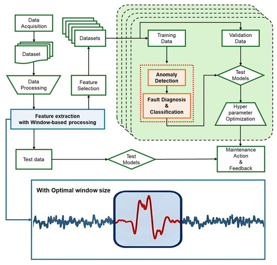
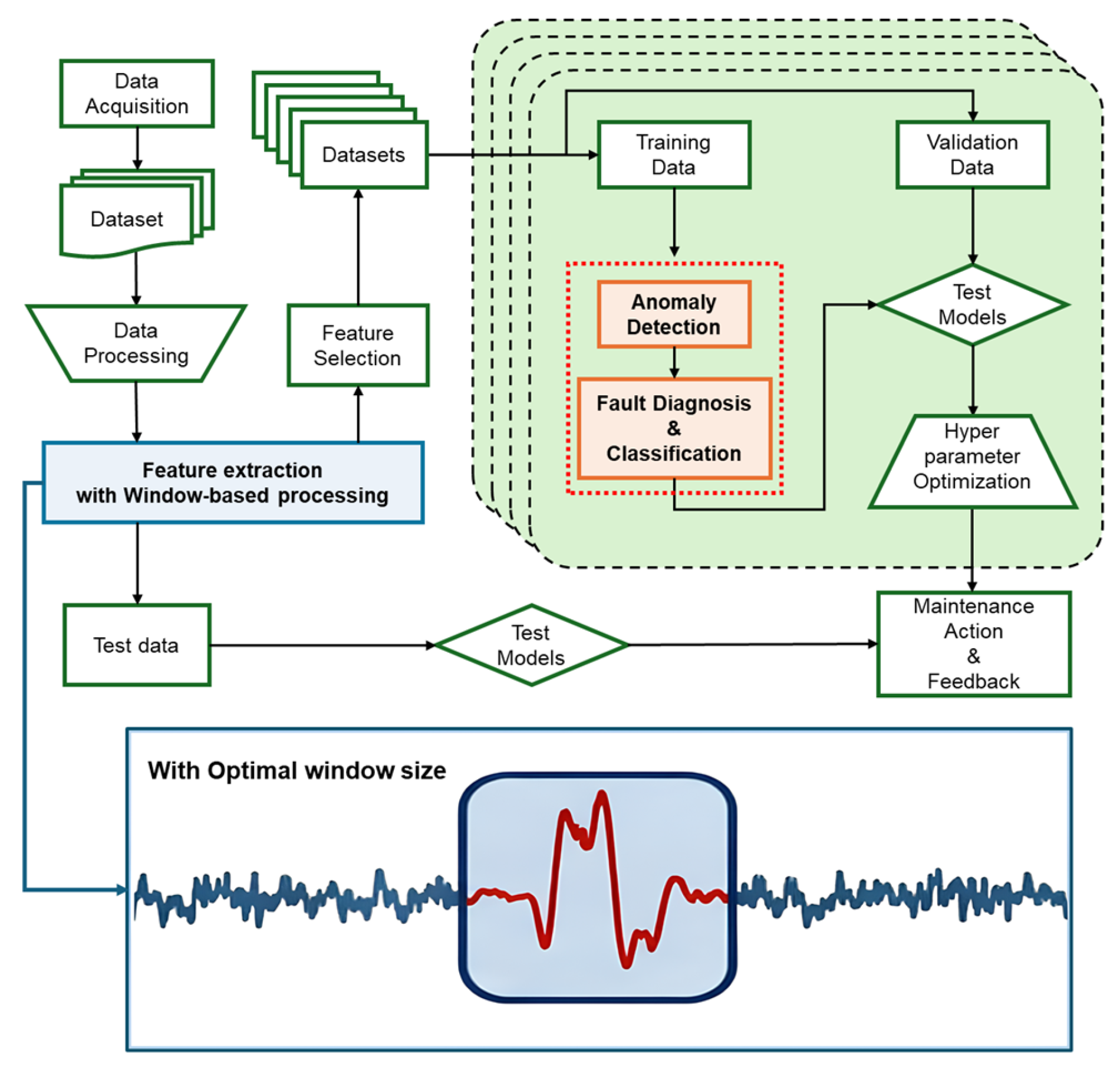
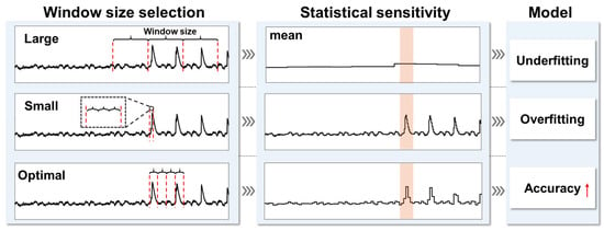
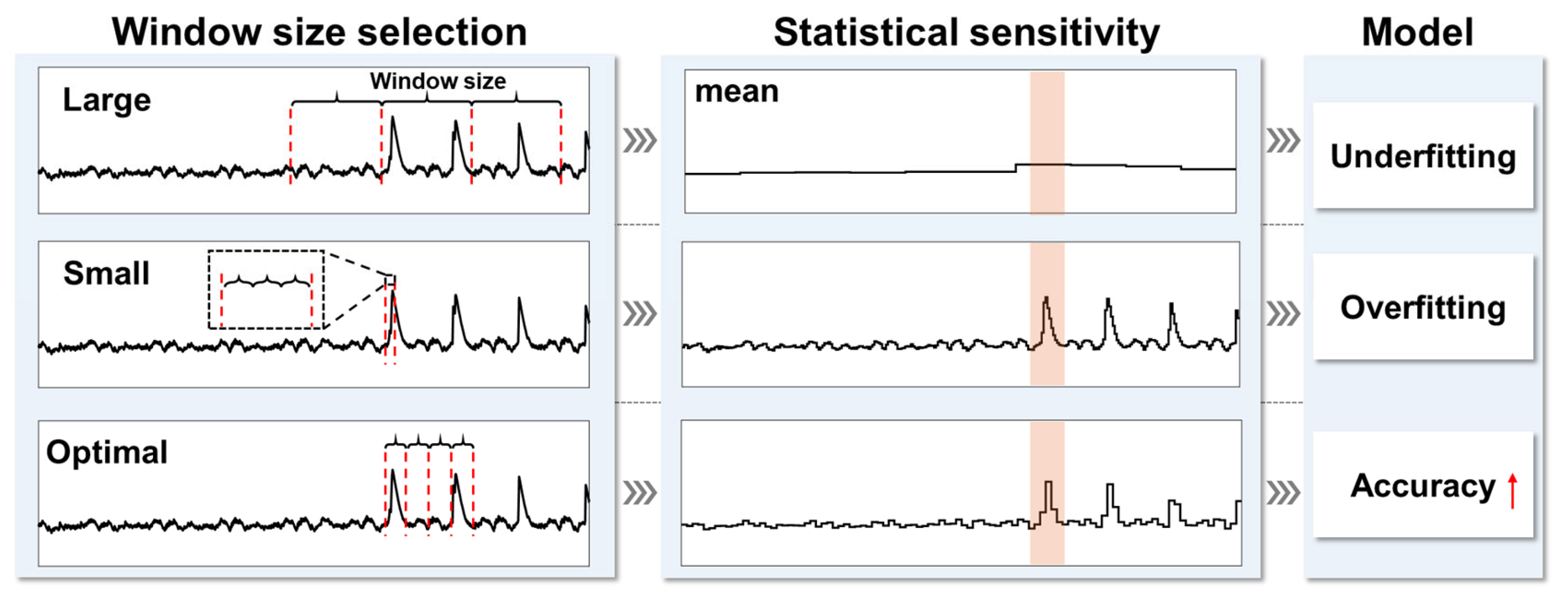
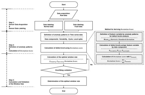
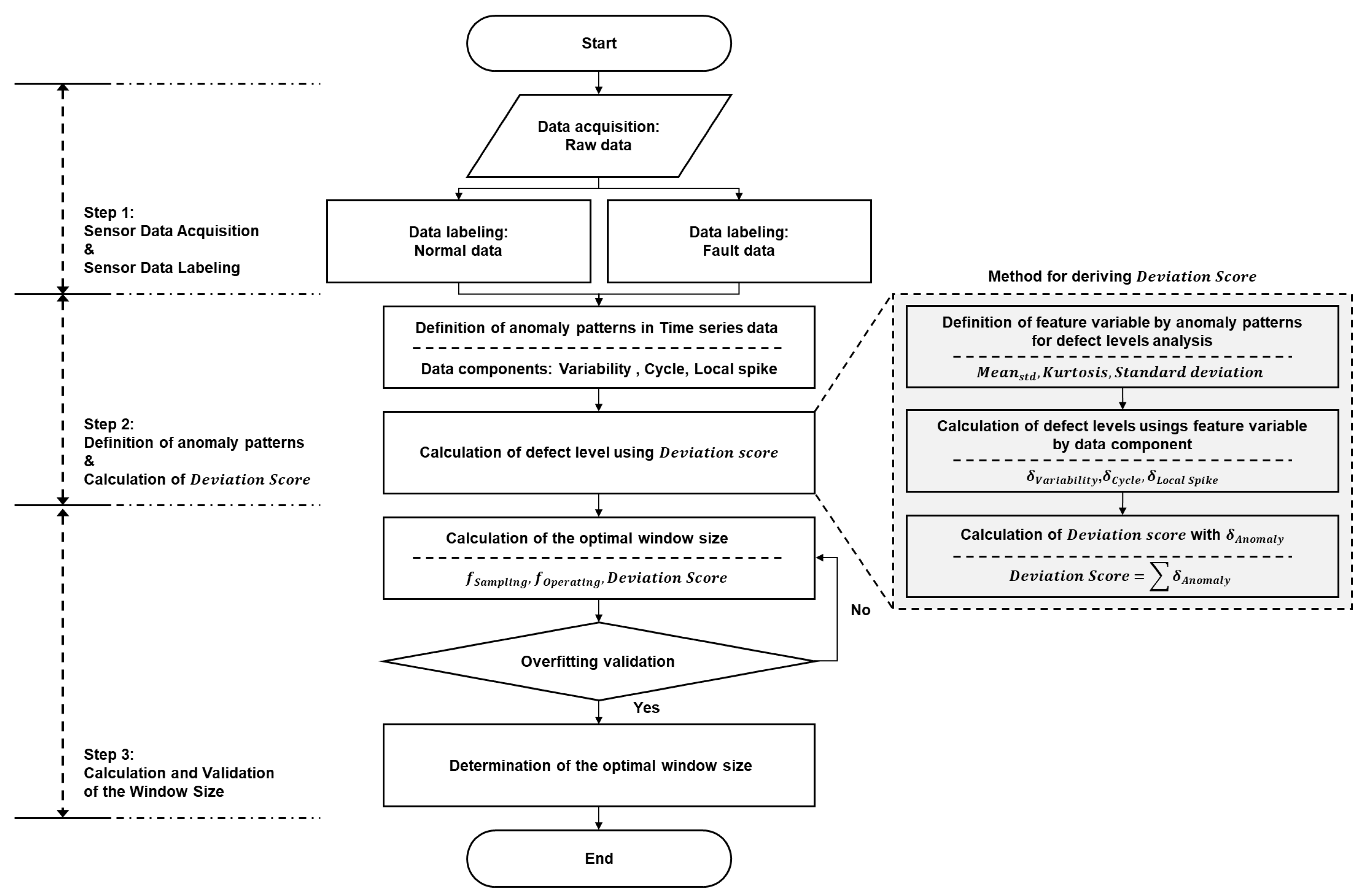
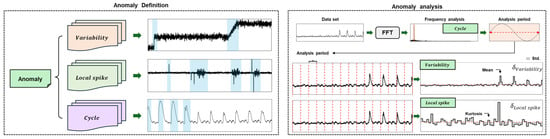
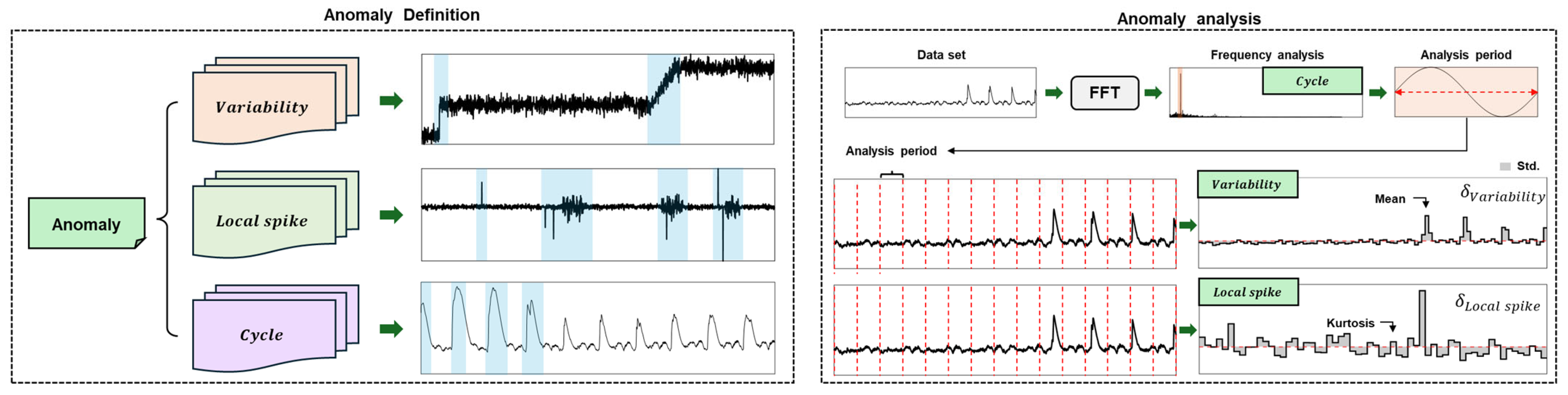
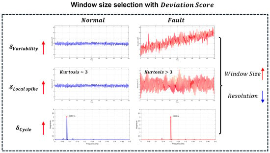
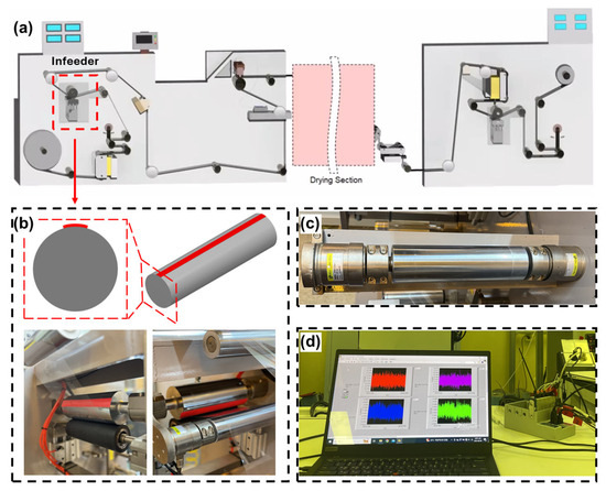
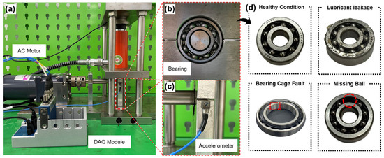
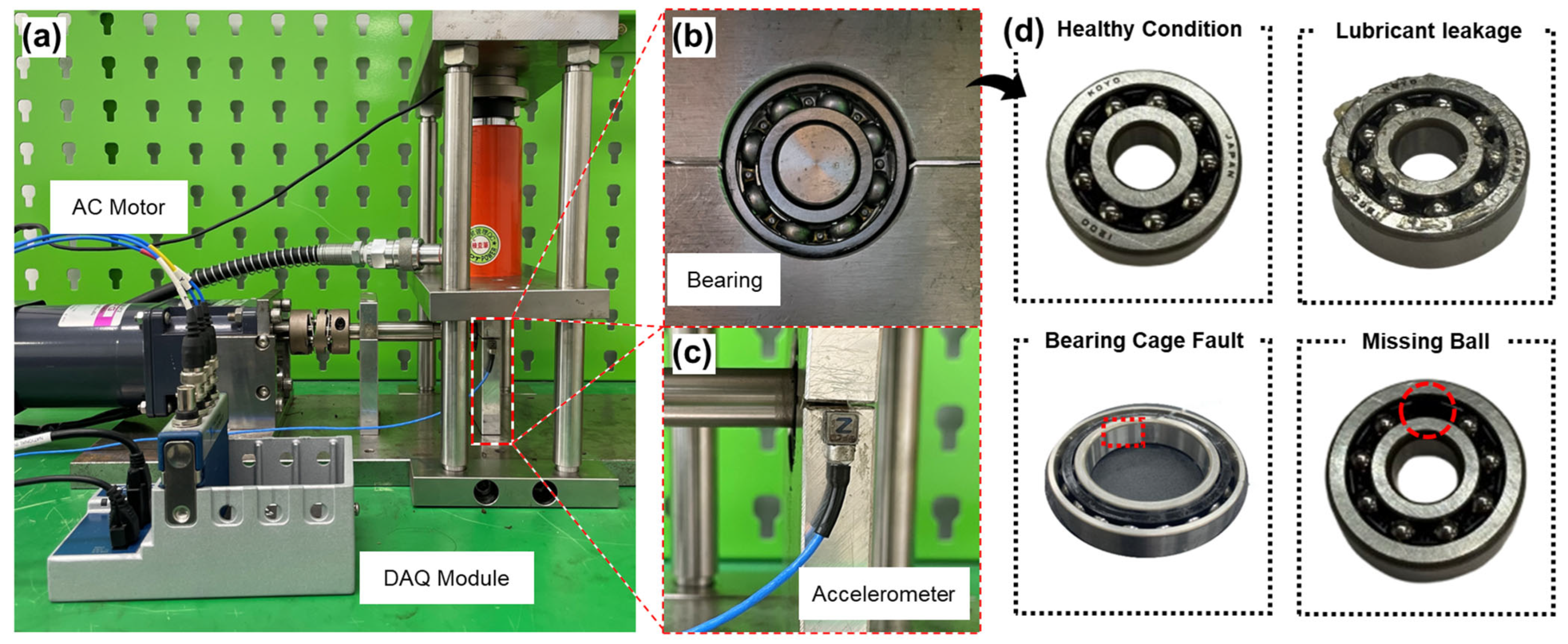
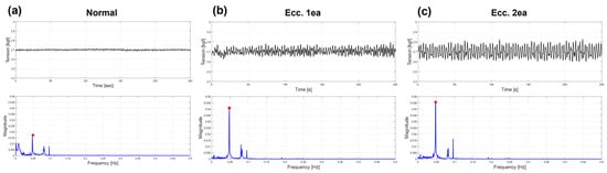
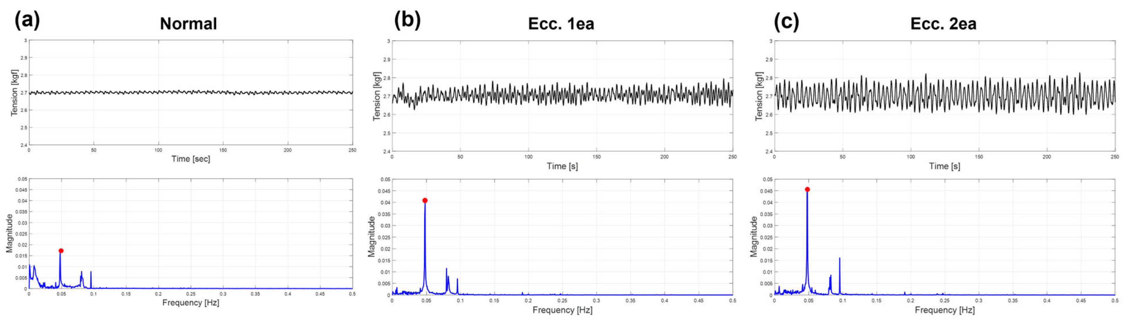
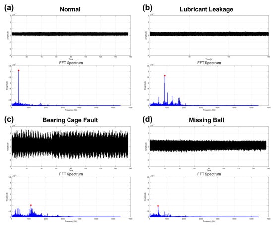
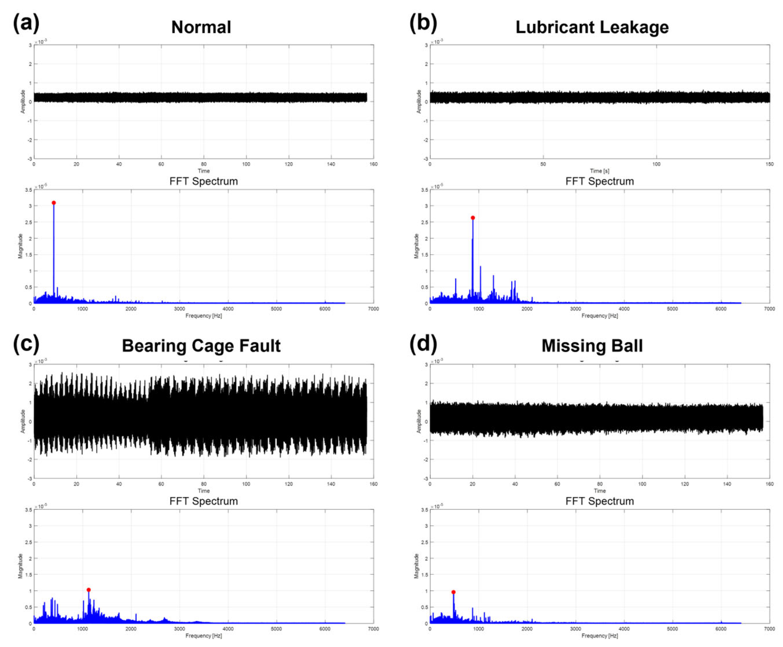
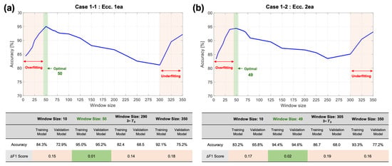
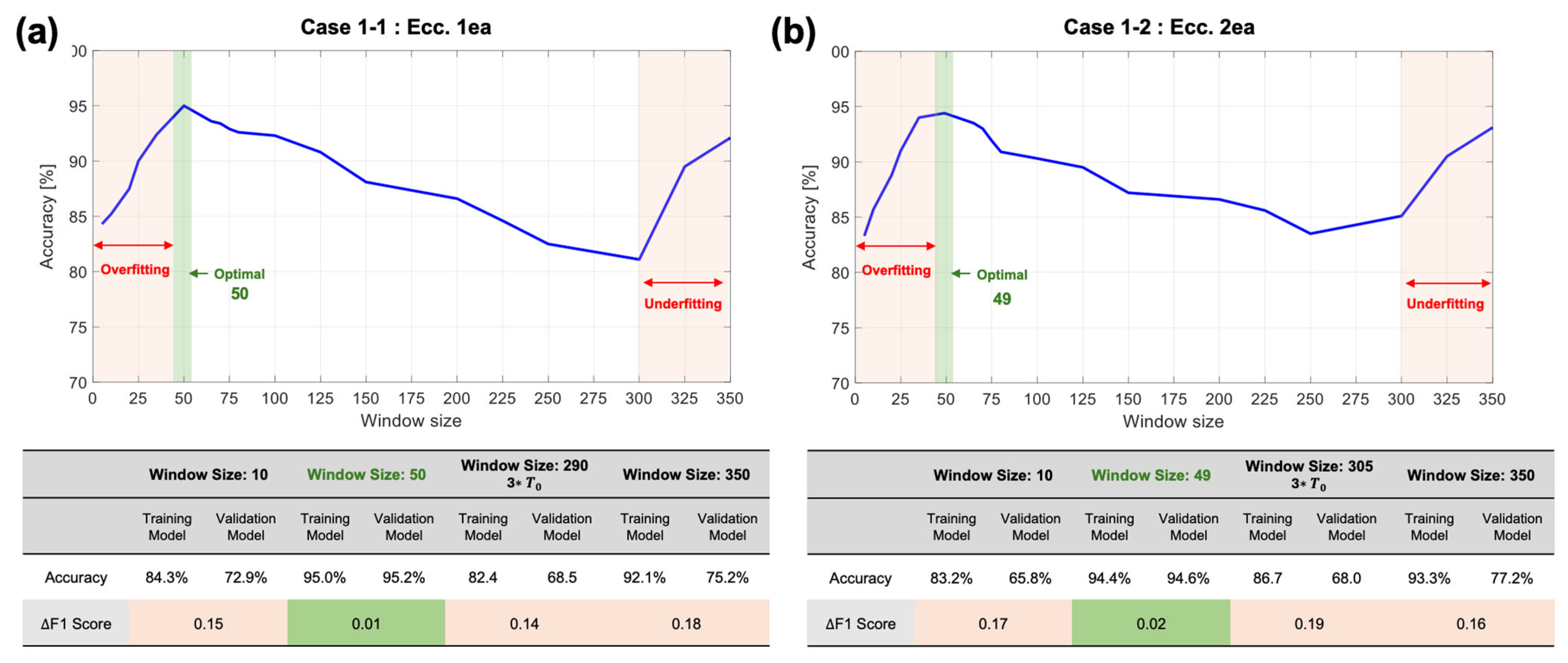
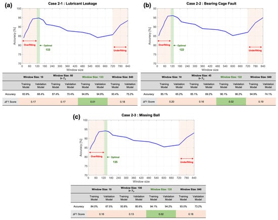
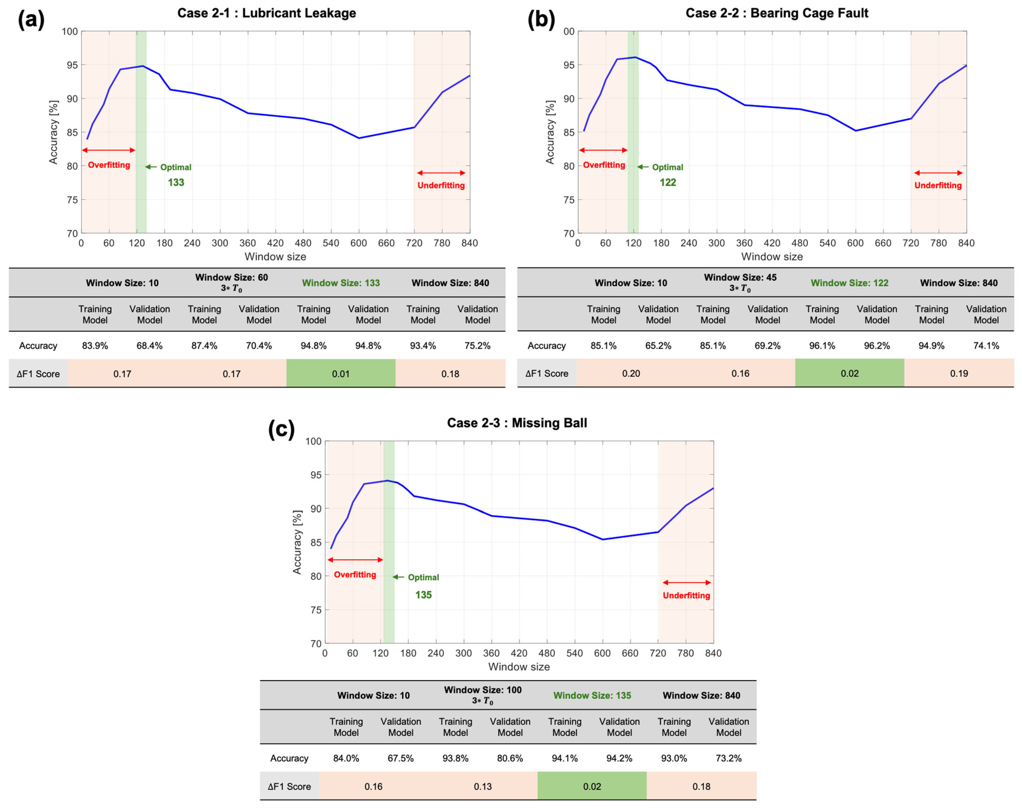

Disclaimer/Publisher’s Note: The statements, opinions and data contained in all publications are solely those of the individual author(s) and contributor(s) and not of MDPI and/or the editor(s). MDPI and/or the editor(s) disclaim responsibility for any injury to people or property resulting from any ideas, methods, instructions or products referred to in the content. |
© 2026 by the authors. Licensee MDPI, Basel, Switzerland. This article is an open access article distributed under the terms and conditions of the Creative Commons Attribution (CC BY) license.