


Abstract
Parametric tiered-seating design can be framed as a constrained multi-objective optimization problem in which a low-dimensional decision vector is evaluated by a deterministic operator with sequential feasibility rejection and visibility constraints. This study introduces an oracle-preserving, learning-assisted screening workflow, where a multi-output multilayer perceptron (MLP) is used only to prioritize candidates for evaluation. Here, multi-output denotes a single network trained to predict the full objective vector jointly. Candidates are sampled within bounded decision ranges and evaluated by an operator that propagates section-coupled geometric state and enforces hard clearance thresholds through a Vertical Sightline System (VSS), i.e., a deterministic row-wise sightline/clearance evaluator that enforces hard clearance thresholds. The oracle-evaluated set is reduced to its mixed-direction Pareto-efficient subset and filtered by feature-space proximity to a fixed validation reference using nearest-neighbor distances in standardized 11-dimensional features, yielding a robustness-oriented pool. A compact shortlist is derived via TOPSIS (Technique for Order Preference by Similarity to an Ideal Solution; used here strictly as a post-Pareto decision-support ranking rule), and preference uncertainty is assessed by Monte Carlo weight sampling from a symmetric Dirichlet distribution. In an archived run under a fixed oracle budget, 1235 feasible designs are evaluated, producing 934 evaluated Pareto solutions; proximity filtering retains 187 robust candidates and TOPSIS reports a traceable top-30 shortlist. Stability is supported by concentrated top-k frequencies under weight perturbations and by audits under single-feature-drop ablations and tested rounding precisions. Overall, the workflow enables reproducible multi-objective screening and reporting for feasibility-dominated seating design.
Keywords:
multi-objective optimization; surrogate-assisted screening; deterministic oracle; Pareto efficiency; robustness diagnostics; feasibility constraints; stadium seating; sightline clearance MSC:
90C29—multi-objective and goal programming
1. Introduction
Tiered grandstand seating can be posed as a constrained multi-objective optimization problem in which a low-dimensional decision vector drives a deterministic generator. The generator propagates geometry row-by-row, applies sequential rule checks, and discards infeasible candidates as soon as a violation occurs. In the present study, section coupling is handled explicitly through an inherited boundary state at section transitions. Feasibility is further enforced at seat level through a section-coupled Vertical Sightline System (VSS) with hard clearance thresholds. As a result, feasibility and objective outputs are produced by a deterministic evaluation operator, rather than by closed-form macro approximations.
From an optimization perspective, this is a typical computationally expensive multi-objective setting. Even under deterministic evaluation, runtime is dominated by repeated feasibility screening and row-wise state propagation, and the feasible region may be sparse. This computational setting motivates the following brief overview of surrogate-assisted multi-objective optimization methods that reduce expensive evaluation calls while preserving Pareto-relevant progress. Accordingly, the literature overview below is focused on surrogate-assisted multi-objective workflows that reduce expensive oracle calls while keeping Pareto trade-offs explicit and reportable. Multi-objective optimization is well suited to such problems because it seeks Pareto-efficient trade-offs instead of a single optimum [1,2]. A design is Pareto-efficient (non-dominated) if no other feasible design improves at least one objective without worsening another under the mixed-direction mask. Here, the Pareto structure is not obtained through evolutionary population updates. Instead, it is extracted from an oracle-evaluated set generated by an iterative, surrogate-assisted screening loop. Surrogate-assisted strategies are commonly used to reduce the number of expensive evaluations while still making Pareto-relevant progress. A learned model helps identify which candidates are worth forwarding to the evaluator next [3,4,5].
In this study, “optimization” is operationalized as budgeted construction of an oracle-evaluated design set and its mixed-direction Pareto extraction, whereas TOPSIS is used only for post-Pareto decision support within the admissible robust pool. A central methodological commitment of this article is oracle preservation. The surrogate model is used only to prioritize candidate designs. All reported objective values, and all downstream Pareto and decision computations, rely exclusively on deterministic oracle evaluations. This makes the validity boundary explicit. Learning accelerates exploration under a fixed evaluation budget, but it neither replaces the evaluator nor introduces surrogate-predicted objectives into reported results. Conceptually, the approach follows surrogate-based optimization and response-surface frameworks in which a learned model informs sampling or selection, through a transparent ordering heuristic used solely to decide which candidates receive oracle evaluation next, while truth evaluations are retained for accepted points [4,5].
Once the oracle-evaluated set is assembled, the workflow extracts Pareto-efficient points under mixed minimization/maximization directions and then adds a robustness-oriented decision layer. Specifically, Pareto-efficient points are filtered by feature-space proximity to a fixed validation reference, operationalizing an OOD-avoidance criterion in the engineered feature representation rather than in objective-space distance. A compact shortlist is then produced using TOPSIS as a transparent multi-criteria decision rule, complemented by weight-uncertainty diagnostics that quantify how shortlist membership changes under preference variation [6]. Finally, because results are communicated through rounded numerical fields, the study includes controlled rounding-sensitivity checks. This step is motivated by the practical reality that rounding is intrinsic to floating-point computation and can affect reported values and derived identifiers if not audited [7].
Overall, the article contributes an end-to-end, reproducible workflow for learning-assisted yet oracle-preserving multi-objective screening of deterministic, feasibility-dominated tiered-seating configurations. The key methodological and reporting contributions are summarized below.
- Oracle-preserving screening: the surrogate is used only to prioritize candidates, while all reported objectives and feasibility outcomes remain strictly oracle-computed.
- Deterministic, section-coupled evaluation: a VSS-based evaluator that propagates row-wise geometric state across coupled sections and tier transitions with feasibility-driven early rejection.
- Explicit multi-objective reporting: Pareto-efficient solutions are extracted from the oracle-evaluated set under a mixed-direction mask, making trade-offs traceable under a fixed evaluation budget.
- Validation-anchored robustness layer: feature-space proximity gating to a fixed validation Pareto reference (OOD avoidance in engineered features), yielding an admissible robust pool.
- Transparent post-Pareto decision support: TOPSIS ranking within the robust pool, complemented by Dirichlet Monte Carlo weight sampling for preference uncertainty stability.
- Reporting-grade stability audits: offline feature-drop ablation and rounding-sensitivity checks, plus supplementary diagnostics on screening alignment and surrogate-family choice, without additional oracle evaluations.
2. Materials and Methods
To improve readability, we first clarify the key technical terms and abbreviations used consistently throughout the Methods and the algorithmic descriptions. These definitions are provided for clarity and are used consistently across the subsequent problem formulation, screening workflow, and reporting diagnostics.
Key terms and abbreviations: MLP: multilayer perceptron (feed-forward neural network surrogate). Multi-output MLP: a single network predicting multiple objectives jointly. VSS: Vertical Sightline System, the deterministic row-wise sightline/clearance evaluator enforcing hard clearance thresholds. TOPSIS: Technique for Order Preference by Similarity to an Ideal Solution, used only for post-Pareto ranking within the robust pool. Pareto-efficient: non-dominated under the mixed min/max direction mask. TA: target analysis for objective-set selection. SA: sensitivity diagnostics (feature-drop ablation and rounding audits) for stability reporting, without additional oracle evaluations.
All experiments and analyses throughout the study were implemented in Python (v3.14.2) using NumPy (v2.4.1), pandas (v2.3.3), SciPy (v1.17.0), and scikit-learn (v1.8.0). Visualizations were generated with Matplotlib (v3.10.8) and Seaborn (v0.13.2), with auxiliary utilities including joblib (v1.5.3), tqdm (v4.67.1), and matplotlib-venn (v1.1.2). Interactive analyses were conducted in Jupyter Notebook (v7.5.2)/JupyterLab (latest stable release).
2.1. Problem Setup and Decision Vector
In simple terms, we automatically generate many alternative tiered-seating layouts and test each one using a rule-based simulator that checks basic buildability and sightline quality. Any design that violates the rules is discarded immediately, so only feasible options remain. From this feasible set, we then identify a small shortlist of strong candidates that balance the main performance trade-offs, so a designer can review a few defensible “best-compromise” solutions instead of thousands of raw alternatives.
We consider a bounded decision vector x = [N0, Z, N1, N2, N3, N4] ∈ Ω where each component lies within prescribed ranges. A deterministic evaluator (oracle) generates a coupled tiered-seating geometry row-by-row, enforces feasibility via sequential rule checks and VSS clearance thresholds, and returns feasibility (feas(x) ∈ {0, 1} together with an objective vector . The optimization goal is to construct, under a fixed oracle-evaluation budget, an oracle-evaluated set and its Pareto-efficient subset under mixed directions [min, max, max, min], where f1 and f4 are minimized and f2 and f3 are maximized. The surrogate model is used only to prioritize which candidates are forwarded to ; all reported results remain oracle-computed.
2.1.1. Block Decomposition and Labels
The grandstand configuration is generated as a two-tier seating system. The first tier is decomposed into three consecutive stand sub-sections, and the second tier is represented as a single stand sub-section, yielding four block-level outputs. The workflow stores block-specific datasets with suffixes 2, 3, 4, 5 where 2–4 correspond to the three first-tier sub-sections and corresponds to the second tier (dataset suffix 5 corresponds to the second-tier block and stand section 4 in the geometric sequence).
2.1.2. Decision Vector, State, and Outputs
The generator is formulated as a deterministic evaluation operator embedded in a constrained multi-objective optimization setting. Let x ∈ Rdx denote the decision vector (variables directly controlled by the search algorithm), s denote intermediate state variables required to propagate the tier construction, and y denote objective outputs used in the optimization stage. The workflow is:
where feas(x) ∈ {0, 1} indicates whether all rule-based feasibility checks are satisfied. This “feasibility-driven rejection” is equivalent to enforcing inequality constraints and is consistent with standard constraint-handling practice in evolutionary optimization [8]. Only x is search-controlled, whereas the propagated geometric state, clearance sequences, feasibility, and exported descriptors are produced deterministically by (Table 1).
Table 1.
Mapping of decision variables, deterministic state, feasibility constraints, and exported descriptors in evaluator ε(x).
In this study, we explicitly separate the decision space from deterministic intermediate outputs and optimization targets. The decision vector x contains only design-controllable parameters that drive the tier generator and row progression. All geometric/visibility quantities computed deterministically per row and then aggregated (e.g., Ddis, Rdis, VVA, ES, C-values, and their maxima) are collected into an intermediate output vector z. The optimization target vector y (4-objective set) is computed downstream from z through deterministic aggregation operators. From a multi-objective optimization perspective, only x constitutes the decision variables, while z and y are outputs (with z intermediate). This matches the canonical multi-objective formulation “minimize f(x) subject to x ∈ S” where x is the decision vector and S (equivalently Ω) is the feasible set defined by constraints [9].
2.1.3. Depth Terms and Baseline
For each block i ∈ {1, 2, 3, 4}, a depth-like variable Ti is computed from the row-rise decision Ni and the fixed slope βi:
A baseline (first row) reference depth T0 is computed deterministically from (Z, N0) and fixed constants (h, B) in the Tier-1 codes:
This T0 belongs to s(x) (intermediate state) because it is deterministically produced inside .
2.1.4. Feasibility Rules: Tier-1 and Tier-2
Feasibility is enforced via sequential rule checks. Candidates failing any rule are rejected (feas(x) = 0); otherwise, they are recorded (feas(x) = 1).
- Piecewise minimum depth constraints (Tier-1); for i ∈ {1, 2, 3}, the generator enforces a minimum depth threshold depending on the sampled Ni:
- Monotonic progression constraints (Tier-1);
- Vertical sightline clearance (C-value); for each first-tier block, a clearance-type metric Ci is computed and thresholded. C-value is employed as a micro-level visibility metric, expressing the vertical separation between the line-of-sight of a spectator and the eye line of the immediately preceding spectator along the section plane. In practice, a commonly circulated closed-form expression:
This quantity serves two purposes in the VSS. It provides an explicit feasibility check against the section threshold τ2 at the entry of the recurrence, and it fixes the initial section-plane slope used by the subsequent row-wise updates that generate the clearance sequence for the first segment. Specifically, each section i is initialized by the terminal geometric state of the previous section, represented by the maxima of cumulative distance sequences: which are computed from the prior section’s row-by-row accumulators (Ddis, Rdis) and then used as boundary conditions for the next section. This state-coupled construction is consistent with the notion that micro-level viewing performance must be evaluated seat-by-seat (or row-by-row) rather than by a single macro approximation [12,13]. Given a candidate design’s section-specific riser Ni and tread Ti (with Equation (2)) the first-row clearance of the next segment is computed by the following section-coupled expressions (using max Dprev, max Rprev as inherited boundary conditions):
Before introducing the second-tier clearance computation (C4), the generator calibrates the second-tier first row (base) depth term T02, which acts as the tier-transition horizontal offset that seeds the upper-tier section plane. In the implementation, T02 is computed from the inherited terminal state of the preceding section (max Dprev, max Rprev), the cantilever translations (canth, cantv), and the fixed constants B and h, and is optionally scaled by a reduction coefficient k to control the resulting depth magnitude:
To avoid under-populating the upper-tier design space and to keep the first-row depth of the second tier within an “ideal” operational range, the generator performs an internal scenario study over six cantilever cases. For each scenario, the distribution of resulting T02 values and the number of feasible second-tier designs are evaluated. The pair (canth, cantv) = (120, 300 cm) is selected because it yields a broader and more usable T02 range and a larger count of feasible upper-tier alternatives, thereby strengthening the coverage of the optimization-ready dataset while maintaining consistent tier-transition geometry. Following this calibration, canth and cantv are fixed for the remainder of the pipeline to prevent scenario-induced confounding in the surrogate and optimization stages. In other words, upper-tier variability is intentionally attributed to the decision-linked tier parameters and to the inherited boundary state (max Dprev, max Rprev), while the cantilever scenario is treated as a controlled setting.
For the upper tier (section 4 in the final tier, denoted “5” in the datasets), the formulation additionally incorporates the tier transition offsets and the section base depth T02 via the cantilever terms canth, cantv:
These expressions preserve the same geometric principle as the standard C-value relation (similar-triangle/gradient consistency in the section plane) while remaining valid under segment-dependent (Ni, Ti, βi) and tier offsets.
Second-tier monotonicity and clearance constraints (Tier-2); the constraint given below is enforced for the same reason as the corresponding first-tier depth constraints. It prevents unrealistically shallow upper-tier rows and stabilizes the section-plane slope so that clearance values remain in an “ideal” regime under the VSS. Practically, this constraint also ensures that the clearance recurrence terminates after a finite number of rows, yielding designs with a controlled, finite row count rather than unbounded growth ().
2.1.5. Row-Wise Clearance via VSS
Beyond the first row, the clearance values are generated row-by-row using a deterministic recurrence that updates the cumulative section-plane distances and recomputes clearance from the updated sightline slope. For a given section i, let Rk and Dk denote the cumulative state at row k. Starting from the section initialization (either (R0, D0) inherited from max Dprev, max Rprev or its tier-adjusted counterpart), the notebook implementation applies:
Beyond the first row, this recurrence is applied to produce the list-valued clearance outputs stored in the datasets as C_values (section 2), C2_values (section 3), C3_values (section 4), and C4_values (section 5). The iteration is terminated when the newly computed clearance falls below the section-specific threshold τi, thereby enforcing that consecutive spectators maintain a non-trivial, threshold-controlled clearance margin throughout the feasible portion of each section. In this way, the VSS establishes a numerically consistent mechanism that respects variable row geometry and rake, carries forward the prior section state through max Dprev, max Rprev, and maintains clearance above target levels to sustain a meaningful separation between successive sightlines across the generated seating configurations [10,11,12,13].
2.1.6. Clearance (C) Thresholds as Constraints
In the proposed Vertical Sightline System (VSS), clearance thresholds are imposed as hard feasibility constraints rather than as post hoc quality scores. For each section i, we define a section-specific clearance floor τi (in cm) and require both the first-row clearance and the entire row-wise clearance sequence to satisfy:
- First-row feasibility: Ci,0 ≥ τi
- Sequential feasibility: Ci,k ≥ τi
The recurrence is terminated at the first violation (i.e., when the next computed clearance drops below τi), and the resulting terminal row index is retained as a discrete descriptor of feasible section extent. In the implemented generator, τi is set to {9, 12, 15, 12} for sections {2, 3, 4, 5}, respectively. These values are treated as model hyperparameters that operationalize minimum sightline separation targets under variable (Ni, Ti, βi), enabling consistent feasibility screening across the generated design set while preserving the common geometric principle underlying classical C-value expressions [10,11,12,13].
Iterative surrogate-assisted screening procedure (ISAS) and target analysis (objective-set selection—TA) stages operate on section-level summary descriptors extracted deterministically from the row-wise state trajectories {Rk, Dk, Ck}. For each section i, the generator stores:
- Clearance list Ci = [Ci,0, Ci,1,…, Ci,ni−1]
- Cumulative distance lists Ri and Di
- Terminal maxima and feasible row count:
maxRi = max(Ri) (exported as max_Rdis)
maxDi = max(Di) (exported as max_Ddis)
ni = ∣Ci∣ (exported as max_row_no)
From these stored sequences, we compute the section-level clearance statistics used downstream:
- Mean clearance:
- Clearance dispersion:
These are recorded as standardized target columns in Stage TA (e.g., C4_values_5_mean_standard, C4_values_5_std_standard) after the preprocessing steps (power transform and scaling).
The tuple (maxDi, ni, μ(Ci), σ(Ci)) jointly captures:
- a geometric reach proxy (maxDi) tied to the section-plane accumulation,
- a discrete feasible extent proxy (ni) resulting from threshold-controlled termination,
- a central tendency of sightline quality (μ(Ci)),
- and its uniformly/robustness (σ(Ci)) across rows.
Because each downstream section is initialized using the upstream terminal state (max Dprev, max Rprev), these summaries remain structurally coupled across sections, while still being compact enough to serve as stable targets for surrogate learning and multi-objective screening (Stage TA/ISAS). In particular, the final section (5) outputs are used as the primary optimization-facing target set in the subsequent stages, since they embed the upstream constraints through the VSS boundary propagation mechanism and the tier-transition offset (T02).
2.2. Chain-Consistent Filtering
Independent outlier removal at each block can break cross-block continuity (i.e., a design alternative retained in block 2 may not be present in 3, etc.). To avoid propagating inconsistent rows into learning/optimization stages, the workflow enforces reference-consistent filtering and adaptive downsampling to target sizes, producing the datasets Filtered_ALL_* and Hybrid_ALL_*.
Let b ∈ {2, 3, 4, 5} denote the block suffix. For b > 2, the current block dataset contains reference columns (max Rb−1, max Db−1) from the previous block, stored explicitly as:
- for b = 3: (max_Rdis_1.1, max_Ddis_1.1),
- for b = 4: (max_Rdis_1.2, max_Ddis_1.2),
- for b = 5: (max_Rdis_1.3, max_Ddis_1.3),
- while the kept previous-block dataset uses (max_Rdis, max_Ddis). Define the kept key set from the previous processed block:
Then the reference-consistent subset of the current raw dataset is:
This step is a deterministic feasibility consistency operation across linked subproblems.
2.2.1. Hybrid Scoring and Target Sizes
After reference filtering, the workflow enforces block-wise target sample sizes are = (3028, 2290, 1577, 1152). For each block, the scoring uses the 2D feature vector:
chosen because it compactly reflects the discrete feasible extent of the section and the geometric reach on the section plane.
Mahalanobis distance component: the Mahalanobis distance is computed as [14]:
The implementation assigns categorical labels using fixed thresholds:
Mean pairwise Euclidean distance component: For each observation i, the mean distance to all other observations in the same block is:
Block-specific thresholds are applied to (Table 2), producing “Normal/Optional/Outlier” bands.
Table 2.
Chain-consistent filtering configuration (as implemented).
K-Means cluster deviation component; a K-Means model is fit on standardized u and each point receives a cluster label. The K-Means family is the standard least-squares clustering model typically attributed to Lloyd’s formulation [15]. The optimal cluster count is selected by combining; an elbow heuristic computed on inertia, the maximum silhouette score, where the silhouette index follows Rousseeuw. Silhouette is referenced here because it is the explicit criterion used in the implementation [16]. Min–max normalization and composite score; each component is min–max normalized:
The composite score used for ranking is:
where dC(i) is the distance-to-centroid term induced by the fitted K-Means clusters. Finally, for each block b, the workflow retains the lowest-scoring nb observations:
2.2.2. Cross-Block Fusion into the Final Optimization Table
After stabilization, chain-consistent filtering stage performs a final consistency pass and merges the four block-level stabilized datasets into a single design table. The fusion is performed by iteratively intersecting upstream/downstream samples using their (max D, max R) key pairs (with rounding applied to mitigate floating mismatches). Specifically, the code:
- Drops diagnostic columns used only for filtering (e.g., K-Means cluster id and distance-based diagnostics) and also removes selected block-specific intermediate columns that would be redundant in the fused table.
- Renames all remaining variables with a consistent prefix and block suffix:
- Concatenates the four aligned blocks column-wise to form the final dataset.
The resulting consolidated table B4_Total.csv contains 1152 rows and 66 columns in the provided output, and is the canonical input to downstream learning and multi-objective screening stages.
The consolidation steps in the early stages are not merely data cleaning but a consistency-preserving construction of the discrete design space required before learning-based multi-objective optimization. Surrogate models assume a one-to-one correspondence between each design row and a single, well-defined alternative; violations of cross-block chain consistency yield misaligned feature–objective pairings and make the learned mapping x → y ill-posed. The key-based filtering and intersection therefore function as an implicit feasibility/consistency constraint that stabilizes subsequent surrogate training, Pareto screening, and multi-criteria ranking, in line with constraint-handling and surrogate-assisted search literature [3,8].
2.3. Target Analysis and Objective-Set Selection—TA
The aim of Stage TA is to define a target/objective set that is structurally meaningful with respect to the deterministic generator, and empirically learnable from the chosen decision-space descriptors, so that subsequent learning-assisted optimization steps remain stable and reproducible. (TA denotes the target/objective-set selection stage used to define a learnable and decision-relevant objective vector for downstream screening.)
In the adopted B4_Total dataset, the grandstand is composed of four consecutive blocks, and each block introduces its own block-specific geometric state and performance descriptors. In principle, this yields a 16-dimensional objective description if the same four block-level performance summaries are retained for each block. However, surrogate-assisted search and downstream decision support benefit from objective sets that are both learnable and decision-relevant, particularly under limited evaluation budgets and when the surrogate is retrained iteratively [17,18,19].
To justify the objective set used in Stage ISAS, two alternative multi-output learning formulations were evaluated in the provided target-analysis workflow. It contains a 16-target ([max D and max(row count) as reach/extent proxies; μ(C) and σ(C) as quality/robustness proxies]) MLP model trained to predict performance summaries for all four blocks simultaneously, and a 4-target MLP model trained only on the second-tier (last-block/5) performance vector. The motivation for privileging the final block is structural. Section 5 variables embed the upstream constraints via deterministic state propagation, so they carry information about earlier sections while remaining compact. To improve numerical conditioning, the implementation applies a Box—Cox power transform (where applicable) to the strictly positive max D and max(row count) columns across all sections, then produces standardized variants.
To evaluate which target set is more learnable from x, Stage TA performs:
- Input preprocessing and dimensionality reduction; the preprocessed dataset has shape (1152, 141) in the provided run, including multiple scaled/standardized variants. PCA is then used to compress inputs to 7 components, with a reported explained variance of approximately 0.99997 for the chosen components [20].
- MLP surrogate regression. A multi-output MLP regressor with hidden layers (64, 32), ReLU activations, and SGD optimization is trained with a manual epoch loop (warm-start, max_iter = 1 per epoch) and a patience-based stopping logic. The use of MLPs as universal approximators provides a principled justification for this surrogate choice [21].
The comparison output CSV file indicates a strong separation in test R2 performance between the two target formulations in the logged run:
- 4-target MLP: best test R2 ≈ 0.896, test MSE = 0.025902
- 16-target MLP: best test R2 ≈ 0.093, test MSE = 0.162887
This empirical result supports selecting the 4-target set as the optimization-facing target definition, because it yields substantially better surrogate fidelity under the same modeling budget and train/test protocol. The decision is therefore not only conceptual (compactness and structural coupling) but also data-driven (learnability).
2.4. Overview of the Iterative Surrogate-Assisted Screening—ISAS (Oracle) Workflow
The study employs an iterative surrogate-assisted screening procedure (ISAS) to explore a multi-objective design space under a strict budget of deterministic evaluations. The core idea is to use a surrogate model only for candidate prioritization, while preserving an oracle-based validity boundary by computing objective values exclusively through a deterministic evaluator at every accepted design point. Surrogate-assisted strategies of this type are widely used in expensive multi-objective optimization to reduce the number of costly evaluations while maintaining meaningful Pareto progress [17,18]. Although the implementation is tailored to tiered-seating configurations, the algorithmic structure is generic and consists of candidate generation, feature construction, surrogate training, acquisition-based screening, budgeted oracle evaluation, evaluated-set Pareto extraction, and a robustness-oriented decision layer.
For clarity and reproducibility, Figure 1 summarizes the end-to-end workflow, separating process steps executed in the iterative screening loop, data artifacts produced at each stage, and reporting-only reductions that do not affect the evaluated sets. Algorithm 1 provides the core pseudocode for the oracle-preserving ISAS loop, including surrogate training and the acquisition-based ordering used only to decide which candidates receive oracle evaluation next. As emphasized throughout, the surrogate is used exclusively for candidate prioritization, whereas feasibility and all reported objective values are computed only by the deterministic evaluator .
| Algorithm 1. Oracle-preserving ISAS (v4.6) |
|
Figure 1.
Overall framework of oracle-preserving workflow (TA–ISAS–Pareto–proximity gating–TOPSIS–SA).
All computations reported for this stage are based on the archived ISAS true-oracle run (v4.6) executed by the accompanying Python implementation. Run-specific diagnostics (iteration counts, predictive metrics, and decision-layer stability outputs) are reported in the Results and are traceable via the exported tables and figures in the output package.
2.4.1. Decision Variables and Derived Feature Representation
Each candidate configuration is parameterized by a 6-dimensional decision vector () stored in the dataset columns; B4_N0_2, B4_Z_2, B4_N1_2, B4_N2_3, B4_N3_4, B4_N4_5. To support surrogate modeling without invoking the full oracle, the implementation augments each decision vector with fast, analytically derived features (stored and used as u, X_feature_cols), yielding an 11-dimensional feature vector ().
Here, the tread-like quantities T0, T1, …, T4 are computed deterministically using fixed geometric parameters (in cm and degrees) as explained under “problem formulation and decision vector” section. This feature construction is used consistently in three places. They are candidate generation (to attach Ti values), surrogate training inputs, and the design-space proximity metric used in robustness filtering.
2.4.2. Objective Vector and Mixed Direction Mask
The oracle returns a four-objective vector () defined in the Stage ISAS run as:
- f1 = max(Ddis) from Block 5, denoted in outputs as f1_max_Ddis (to be minimized—to reduce average viewing distance and bowl size)
- f2 = max(row_no) from Block 5, denoted as f2_max_row_no (to be maximized—to increase capacity under comparable viewing perimeter)
- f3 = μ(C4), the mean of the Block 5 clearance sequence, denoted as f3_C4_mean (to be maximized—to increase general viewing quality levels)
- f4 = σ(C4), the sample standard deviation of the Block 5 clearance sequence with ddof = 1, denoted as f4_C4_std (to be minimized—to reduce dispersion in clearance quality).
Accordingly, the mixed-direction mask used throughout Stage ISAS is [min, max, max, min].
2.4.3. Iterative Surrogate Training and Budgeted Oracle Evaluations
Rationale for surrogate choice; in ISAS, the surrogate is intentionally used as a low-overhead ranking model rather than a replacement for the deterministic evaluator. This design follows from three characteristics of the problem. Oracle evaluation is expensive due to sequential rule checks and row-wise state propagation, feasibility is sparse so many proposals are rejected early, and the mapping from decision parameters to objectives is nonlinear because of section coupling and tier transitions.
A multi-output MLP trained on engineered 11D features offers a favorable trade-off between expressive power and retraining cost within an iterative loop. In contrast, Gaussian-process or Bayesian surrogates can be less convenient here due to repeated refitting overhead and multi-output handling under heterogeneous target scales, especially when the model is retrained multiple times and used only for screening. Population-based evolutionary multi-objective optimizers are not the focus because the contribution is a budgeted, oracle-preserving screening-and-reporting workflow in which Pareto structure is extracted from oracle-evaluated sets and decision support is applied post-Pareto. Finally, surrogate-predicted objectives are intentionally not used as reported results to preserve a strict true-oracle validity boundary.
Stage ISAS proceeds in a budgeted loop in which the surrogate is retrained each iteration and used to prioritize a larger candidate pool for deterministic oracle evaluation.
Surrogate training protocol (v4.6; per iteration); at iteration t, the surrogate is retrained on the current evaluated set Deval = {()}, where ui ← ϕ(xi) ∈ R11 is the engineered feature vector and are objective values computed only by the deterministic evaluator for feasible designs. The data are split into train/test subsets (test size 0.20) for diagnostic reporting. A feature StandardScaler is fitted on the training subset and applied to both train and test features, and objective-wise scaling is applied to the targets to address heterogeneous magnitudes (Min–Max for , Standard scaling for ); fitted scalers are retained for inverse transformation of candidate predictions. The multi-output MLP (settings reported below) is then fit on the scaled training data and evaluated on the held-out subset using objective-wise R2/MAE/RMSE and parity-style diagnostics (diagnostic only). The trained model is subsequently used to predict ŷ for a larger candidate pool, enabling an acquisition-based ordering that selects the next batch of candidates for oracle evaluation. Importantly, surrogate predictions are used exclusively for candidate prioritization; all objective values used in Pareto extraction, proximity gating, TOPSIS ranking, and stability diagnostics remain oracle-computed.
The surrogate model is an MLP regressor with; hidden layer sizes (128, 64), ReLU activation, Adam solver, L2 regularization α = 5 × 10⁻⁴, learning rate 10−3, and a maximum of 4000 iterations. This choice is consistent with common practices for neural surrogate modeling in expensive optimization loops [17,18,19], and the Adam optimizer is widely used for training deep networks in such settings [22].
2.4.4. Surrogate-Assisted Screening via an Equal-Weight Acquisition Score
Candidate proposals are generated by uniform sampling within a bounded decision hyper-rectangle defined per decision variable and stored in the archived configuration. For each iteration, a candidate pool C is constructed and mapped to the 11-dimensional feature space . Feature vectors are standardized using a scaler fit on the iteration’s training split. The trained surrogate then produces predicted objectives ŷ(x) (in the surrogate’s scaled target space), which are inverse-transformed back to objective units using the stored per-objective scalers.
To prioritize candidates for oracle evaluation, the implementation computes a scalar acquisition score as a transparent equal-weight ordering heuristic. Importantly, in v4.6 the acquisition score is computed in a direction-harmonized minimization space consistent with the mixed objective definition. Let the effective prediction vector be:
where maximization objectives (f2, f3) are sign-flipped so that lower values are preferable in the acquisition ordering, while minimization objectives (f1, f4) are kept as-is. The effective components are then min–max normalized over the candidate pool C and aggregated with equal weights:
where δ is a small constant for numerical stability. Candidates are ranked by s(x), and the lowest-scoring candidates are submitted to the deterministic oracle until the iteration’s feasible evaluation budget is filled (or a resampling cap is reached due to feasibility rejections).
This screening step provides only an ordering for oracle evaluations. The formal multi-objective logic (dominance under the mixed-direction mask) is enforced downstream on the evaluated set during Pareto extraction and subsequent decision steps.
2.4.5. Evaluated Pareto Construction and Reporting Reduction
After each iteration, the evaluated set is filtered to its Pareto-efficient subset using the standard dominance relation under mixed minimization/maximization objectives [1]. In the implementation, dominance is evaluated in a consistent minimization space by sign-flipping maximization objectives prior to the pairwise dominance test. Let the evaluated objective matrix be Y ∈ Rn×4 ordered as [f1, f2, f3, f4]. The direction-harmonized minimization representation is:
and design a is said to dominate design b if component-wise and strict inequality holds in at least one component.
For readability and repository manageability, a reporting-only reduction is generated from the evaluated Pareto set. This reduction does not affect Pareto extraction, proximity filtering, or TOPSIS ranking. The reduction applies grid-based binning in a direction-harmonized, min–max normalized objective space, conceptually aligned with ε-dominance and ε-grid approaches used to obtain well-spread representations of Pareto sets [23]. Specifically, each objective dimension is min–max normalized on the evaluated Pareto set (after direction harmonization), the normalized space is discretized into a fixed number of bins per dimension (nbins), and at most nmax representatives are retained across occupied bins by selecting one representative per bin according to a fixed tie-breaking rule. The resulting reduced set is used exclusively for generating compact Pareto projection plots and supplementary pairwise views.
2.4.6. Proximity Gating Against the Validation Pareto
Stage ISAS includes a proximity filter intended to avoid evaluated Pareto solutions that are excessively distant from a fixed validation reference in the design/feature space, rather than in the objective space. The validation reference pool is the stabilized dataset B4_Total.csv with npool = 1152 designs. A validation Pareto set is extracted from this pool using the same objective definitions and mixed-direction dominance relation as used for the evaluated set.
Proximity is computed in the standardized feature space defined by the 11-dimensional feature vector u = . A StandardScaler is fitted on the validation reference pool features and applied to both the evaluated Pareto and validation Pareto feature matrixes:
For each evaluated Pareto design i ∈ , the nearest-neighbor distance to the validation Pareto is computed as:
The filter threshold is defined by a fixed quantile of the empirical distance distribution with q set a priori (in this work, q = 0.20). The robust pool is then defined as:
This step must be interpreted strictly as a design-space proximity/OOD-avoidance filter anchored to a fixed validation reference. It is not an objective-space distance-to-front criterion.
2.4.7. Robust Multi-Criteria Decision Analysis via TOPSIS and Weight Stability
After proximity gating defines the admissible robust pool, a transparent multi-criteria decision layer is applied to derive a compact shortlist.
In this study, TOPSIS is not used as a multi-objective optimization algorithm or as a design-space exploration method. The multi-objective structure is established upstream by the oracle-preserving screening loop that assembles Deval under a fixed oracle budget and by extracting the evaluated Pareto set under the mixed-direction mask. TOPSIS is applied only after evaluated Pareto construction and validation-anchored proximity gating, as a transparent multi-criteria decision-analysis rule that produces a compact, reportable shortlist from an already non-dominated and admissible pool. Accordingly, comparisons to evolutionary multi-objective optimizers concern the search stage, whereas TOPSIS concerns post-Pareto ranking/decision support within the robust pool [6,24].
Algorithm 2 summarizes the full decision pipeline from evaluated Pareto extraction through validation-anchored proximity gating to TOPSIS ranking and Dirichlet-based weight-uncertainty testing.
| Algorithm 2. Evaluated Pareto → Proximity gating → TOPSIS ranking and Dirichlet stability |
|
For clarity, Figure 2 schematically illustrates the TOPSIS sub-steps (Algorithm 2, Step 5) and the Dirichlet weight-uncertainty loop (Algorithm 2, Step 6) as implemented.
Figure 2.
TOPSIS decision pipeline on robust pool and Dirichlet-based weight-uncertainty testing.
Mixed objective directions are handled by converting the criteria to benefit form and ranking alternatives by the closeness coefficient Ci (Equation (29)) in the standard TOPSIS formulation. Preference uncertainty is assessed via Monte Carlo sampling of criterion weights from a symmetric Dirichlet distribution w(m) ∼ Dirichlet(1, 1, 1, 1) for m = 1, …, nmc, rerunning TOPSIS under each draw, and reporting top-k inclusion frequencies (with k = 10) as a stability diagnostic.
All tables and figures used for this stability reporting are exported by the implementation and referenced in the Results.
2.4.8. Computational Complexity of the ISAS Workflow
Let T denote the number of ISAS iterations, B the feasible batch size added per iteration, and M the candidate multiplier such that the candidate pool size is C = MB (in v4.6, T = 8, B ≈ 120, C = 3000). Let d be the feature dimension (here d = 11) and m the number of objectives (here m = 4). The dominant cost is the deterministic oracle evaluation, because feasibility is enforced through row-wise recurrences with early termination. With a per-section cap of R row updates (here R ≤ 200) and a constant number of sections, one oracle call costs O(R), so the total oracle cost is O(NevalR), where Neval is the number of feasible designs admitted to Deval (e.g., Neval = 1235 in v4.6).
Per iteration, surrogate retraining on nt = ∣Deval∣ points has cost O(I nt W), where I is the number of optimizer steps used by the MLP solver and W is the parameter count of the fixed network architecture. Candidate screening requires predicting objectives for C candidates and thus costs O(CW) per iteration, with additional O(Cd) for feature construction and standardization. Evaluated-set Pareto extraction is based on pairwise dominance checks and has worst-case cost O(m).
After the run, proximity gating computes nearest-neighbor distances from ∣∣ evaluated Pareto points to a validation Pareto of size ∣∣ in d-dimensional standardized feature space. This step is O(∣∣ log ∣∣ + ∣∣ log ∣∣) with tree-based indexing (and O(∣ ∣∣∣d) as a conservative upper bound). TOPSIS on the robust pool is linear in the number of retained alternatives, i.e., O(∣∣m). The Dirichlet weight-uncertainty test repeats TOPSIS for nmc draws and is O(nmc∣∣m) (here nmc = 2000).
Finally, Stage SA reuses the exported evaluated sets to perform reporting-grade ablation and rounding audits and therefore adds only post-processing overhead without introducing additional oracle evaluations.
2.5. Stage SA: Reporting and Audits
This stage (Sensitivity diagnostics—SA) packages the Stage ISAS outputs into summaries and performs two lightweight diagnostic checks (feature-drop ablation and rounding sensitivity) to assess the stability of the decision layer. These steps are reporting and verification utilities and do not modify the evaluated set, the evaluated Pareto set, or the Stage ISAS decision procedure. Accordingly, Stage SA is not an additional optimization stage; it is a reporting and robustness-audit layer intended to improve interpretability, traceability, and reproducibility of the reported results [25].
For completeness, the reporting-grade verification procedures (feature-drop ablation of the proximity filter and rounding-sensitivity audits) are provided as Algorithm A1 in Appendix B.
Additional offline diagnostics for screening alignment and surrogate choice are implemented. Stage SA also includes two lightweight, offline diagnostics that are computed on the archived true-oracle outputs and therefore require no additional oracle evaluations. First, screening alignment is assessed by computing a direction-harmonized, equal-weight acquisition-style score post hoc from oracle-evaluated objectives and quantifying Pareto enrichment among the top-K ranked candidates. Second, a surrogate-family diagnostic compares alternative multi-output regressors under the same feature representation u = ϕ(x), train/test protocol, and objective-wise scaling used in Stage ISAS. Full tabulated results are provided in Appendix B (Table A9 and Table A10) and are reported strictly as screening diagnostics, since all reported objective values and downstream decision artifacts remain oracle-computed.
Offline comparison of acquisition-style ordering rules (no additional oracle evaluations) are implemented. In response to the request for comparing alternative multi-objective acquisition strategies under the same budget, we report an additional post hoc diagnostic computed strictly on the archived true-oracle-evaluated set. Specifically, we re-rank the already oracle-evaluated feasible designs using three mainstream scalarization-style ordering rules applied in a direction-harmonized minimization space. The baseline equal-weight normalized mean used in ISAS v4.6 (ordering only), a weighted Tchebycheff-style criterion, and a penalty-based boundary-intersection (PBI) style criterion. For each rule, we quantify Pareto enrichment by reporting the fraction of evaluated designs that are Pareto-efficient within the top-K positions (K ∈ {50, 100, 200, 300}) and the corresponding lift over the baseline Pareto rate in the evaluated set. Because all scores are computed from oracle-evaluated objectives only, this comparison introduces no new oracle calls and preserves the integrity of the archived results, while still making the relative ordering behavior of common acquisition-style heuristics transparent. The full comparison is provided in Appendix B (Table A11).
2.5.1. Reporting Summaries of Pareto Sets and Shortlist
Stage SA consolidates the core sets produced by Stage ISAS (evaluated set, evaluated Pareto set, validation Pareto set, and the robust pool) into a compact summary of characteristics suitable for direct reporting. The summary includes the governing proximity-filter configuration and objective ranges observed on the evaluated and evaluated Pareto sets. In addition, Stage SA generates a compact set-size visualization to provide a one-glance overview of the pipeline progression from evaluated designs to the final shortlist.
To support traceable decision reporting, Stage SA also compiles a consolidated shortlist summary that includes the shortlist label, TOPSIS rank/score, the design-space nearest-neighbor distance to the validation Pareto (as defined in Stage ISAS), the objective vector, and the decision variables. A supplementary heatmap-style view is produced to visualize the shortlist across objectives and decision variables without introducing additional narrative.
All numerical values and visual outputs generated by these reporting summaries are presented in the Results section and are made available through the associated repository for reproducibility [25].
2.5.2. Feature-Drop Ablation (Proximity)
Stage SA performs a one-at-a-time feature-drop ablation to assess whether robust-pool construction and the downstream shortlist are overly reliant on any single component of the 11D feature vector used in the Stage ISAS proximity filter. Concretely, the analysis is repeated after removing each feature coordinate in turn, and the resulting changes in the robust set and shortlist membership are recorded. Sensitivity analysis is commonly used to identify which parameters or inputs exert the strongest influence on model outputs [26]. Here, the same rationale is applied to a controlled perturbation of the feature representation that drives proximity-based filtering. For each ablation scenario, one feature coordinate is removed, nearest-neighbor distances from evaluated Pareto points to the validation Pareto are recomputed in the reduced feature space, the proximity threshold is redefined using the same fixed quantile rule as in Stage ISAS, the robust pool is reconstructed, and the shortlist is recomputed under the same TOPSIS configuration.
Agreement with the baseline shortlist is quantified using top-k overlap and Jaccard similarity on the top-30 set:
Stage SA reports these agreement metrics and the associated diagnostic visualization in Section 3.
2.5.3. Rounding Sensitivity and Decision-Impact Check
Stage SA exports two rounding-related checks to separate data-integrity risks from decision-layer sensitivity under rounding perturbations.
A collision audit is performed across multiple rounding precisions to verify that rounding of continuous fields does not collapse distinct alternatives into identical stable identifiers. This is motivated by the fact that floating-point results must often be rounded to fit finite representations, and the resulting rounding error is a characteristic aspect of floating-point computation [7]. Collisions are evaluated on both the evaluated set and the evaluated Pareto set across tested precisions. To quantify decision sensitivity, the pipeline recomputes the proximity threshold, reconstructs the robust pool, and re-evaluates shortlist membership under each rounding precision. Agreement with the baseline shortlist is summarized using overlap and Jaccard metrics consistent with Section 2.5.2. Stage SA reports these stability outcomes in Section 3 as evidence that the exported decision artifacts are robust to controlled numerical perturbations.
All Stage SA outputs are archived alongside the code and configuration needed to reproduce them, consistent with reproducible computational research practices [25].
3. Results
3.1. Run Summary Under Fixed Oracle Budget (ISAS v4.6)
The Stage ISAS workflow completed under a fixed budget of deterministic (true-oracle) evaluations and produced a fully traceable set of intermediate and final artifacts. Across the run, the evaluated design set reached n = 1235 oracle-evaluated alternatives, from which an evaluated Pareto set of n = 934 non-dominated solutions was extracted under the mixed-direction mask [min, max, max, min] (Table 3). In parallel, a stabilized validation reference was used to derive a validation Pareto set (n = 769), providing an external anchor for the feature-space proximity filter used to form a robustness-oriented subset of the evaluated Pareto set.
Table 3.
Stage ISAS run outcome and key set sizes (v4.6).
Design-space proximity was enforced by thresholding nearest-neighbor distances in the standardized 11D feature space at the q = 0.20 quantile, yielding a robust pool of n = 187 evaluated Pareto solutions. A final evaluated-only shortlist of k = 30 alternatives was then reported from this robust pool using TOPSIS, complemented by a weight-uncertainty stability analysis based on Monte Carlo sampling (nmc = 2000, top-k recording with k = 10). The resulting set-size progression from evaluated designs to the final shortlist is summarized in Figure 3a. Iteration-wise evaluated-set growth and the corresponding Pareto set sizes across the eight budgeted iterations are provided in Table A1.
Figure 3.
Stage ISAS run overview and surrogate diagnostics (v4.6). (a) Set-size progression from evaluated designs to final shortlist; (b) Surrogate parity on held-out split (diagnostic only; objective values remain oracle-computed); (c) Budget-related run diagnostic summarizing iteration-wise progress under fixed evaluation budget (see Methods for loop settings).
3.2. Objective Distributions and Scale Heterogeneity
The evaluated set exhibits pronounced scale heterogeneity across objectives, which is a defining characteristic of the optimization problem rather than a post-processing artifact. In raw units, the distance-related criterion f1 spans approximately 5570–33,453, whereas the clearance-mean f3 is concentrated in a narrow band (∼12.04–13.87). The capacity-proxy f2 ranges from 4 to 83, and the dispersion criterion f4 from ∼0.085 to ∼1.237. This combination; one broad, heavy-tailed distance term and a comparatively tight clearance-mean term, creates an inherent risk that any naïve scalar aggregation would be dominated by a subset of objectives solely due to magnitude, not preference. Beyond scale, the distributional shape is informative for interpreting subsequent results. The evaluated population contains a relatively large mid-range mass in f2, while higher-capacity outcomes form a minority tail. In contrast, f3 varies modestly in absolute terms but still meaningfully differentiates alternatives because it is derived from row-wise clearance sequences aggregated deterministically. These raw distribution summaries (Table 4; Table A2) therefore contextualize why the run must be interpreted through mixed-direction Pareto structure and a decision layer, rather than single-score reporting.
Table 4.
Objective ranges on evaluated and evaluated Pareto sets (v4.6); Units: f1 in cm, f2 in rows, f3 in cm, and f4 in cm.
3.3. Surrogate Diagnostic Fidelity Under a True-Oracle Loop
The surrogate model is used exclusively to prioritize candidate designs for deterministic evaluation and does not replace the oracle in computing objective values. Its predictive behavior is therefore reported only as a diagnostic check that the screening stage is informative rather than arbitrary. In this role, the held-out parity behavior indicates that the surrogate consistently provides a meaningful ordering signal across objectives, with the strongest agreement for f2 and stable performance for f3 and f4. The most challenging target is f1, which exhibits the largest iteration-to-iteration variability in fit, consistent with its broader range and tail behavior in the raw distributions.
Table A3 quantifies this diagnostic pattern. R2 remains above ∼0.986 for f2 across iterations, while f1 spans a wider range (from ∼0.756 at its weakest iteration to ∼0.943 at the final state). Importantly, the run-level budget summary aligns with these diagnostics. The iteration history (Table A1) shows that best-so-far improvements occur in a stepwise manner and are not synchronized across objectives. For example, the best observed f1 is reached by iteration 3, while the best f4 improves later (iteration 6). Figure 3b compares surrogate predictions vs. oracle-evaluated targets on the held-out split, providing an objective-wise diagnostic of prediction error and bias across the observed range. Figure 3c summarizes run-level progress under the fixed oracle budget by tracking iteration-to-iteration changes in best-so-far (or envelope) indicators derived from the archived outputs, showing when substantive gains occur and whether improvements are synchronized across objectives. Taken together, Figure 3b verifies that the surrogate is informative for screening, while Figure 3c shows how the screened oracle evaluations translate into objective-space progress before Pareto trade-offs are examined in Figure 4.
Figure 4.
Evaluated Pareto projections (v4.6): (a) (f1, f2) plane showing trade-off between maximum viewing distance and maximum row count; (b) (f3, f4) plane showing trade-off between mean clearance quality and its dispersion.
3.4. Evaluated Pareto Structure and Objective Coupling
The evaluated Pareto set captures non-trivial trade-offs under the mixed-direction mask [min, max, max, min] and demonstrates that the oracle-budgeted search does not merely accumulate feasible points, but meaningfully populates competing regions of objective space. The (f1, f2) projection (Figure 4a) exhibits a strong trade-off signature. Capacity-proxy gains are typically associated with increased viewing-distance extent, indicating that under the present decision space and feasibility constraints, higher f2 is rarely achieved without paying a penalty in f1. This coupling is a structural property of the evaluated Pareto set and motivates a decision layer rather than single-objective tuning.
The (f3, f4) plane (Figure 4b) reveals a second, practically important coupling: increases in clearance-mean f3 frequently coincide with increased clearance dispersion f4. Since f3 summarizes overall clearance levels while f4 penalizes non-uniformity across the row sequence, the Pareto set makes explicit that “better on average” can also mean “less uniform,” depending on the configuration. These two planes therefore offer complementary evidence. One reflects a trade-off between geometric extent and the capacity proxy, while the other captures the tension between mean clearance and the dispersion of clearance quality.
For completeness, the scatter plots include additional pairwise projections of the evaluated Pareto set (Figure A1), together with reduced point sets used only to improve plot legibility when the front is visually dense (Figure A2). The reduced set is used exclusively for visualization and does not affect Pareto membership or any downstream decision calculations. In the archived run, the evaluated Pareto set (n = 934) is reduced to 250 representatives using a 25-bin grid per objective (cap 250 points), resulting in 549 occupied bins, and this reduced set is used exclusively for visualization. These supplementary plots are provided for inspection and presentation purposes and do not affect Pareto membership or any downstream decision calculations.
3.5. Proximity Gating Against the Validation Reference
Because the robust pool is defined in feature/design space rather than in objective space, it acts as an explicit guardrail against evaluated Pareto solutions that are non-dominated yet far from the fixed validation reference in the standardized 11D representation. The nearest-neighbor distance distribution is markedly right-tailed (Figure 5a), indicating that a non-trivial subset of evaluated Pareto points lie at substantial feature-space distance from the validation Pareto set even after feasibility-driven oracle evaluation.
Figure 5.
Robust decision-layer diagnostics (v4.6): (a) Distribution of nearest-neighbor distances from evaluated Pareto set to validation Pareto in standardized 11D feature space, used for proximity-based robust pooling; (b) TOPSIS top-k frequency under Dirichlet weight sampling.
The threshold is defined as a fixed quantile of this empirical distance distribution. In v4.6, the 0.20-quantile is ε = 1.077699 (Table A4), which yields a robust pool of n = 187 designs (as also recorded in the Stage SA characteristics summary). The quantile table further clarifies the separation induced by a rule. Distances move from sub-1 values at the lower tail (e.g., Q0.10 ≈ 0.839) to substantially larger values toward the upper tail (e.g., Q0.90 ≈ 3.801). This supports an important reading boundary for later sections: the decision layer operates within the robust pool and therefore reflects a “validated-neighborhood” selection, not a global selection across the full evaluated Pareto set.
3.6. Robust Decision Layer: TOPSIS Shortlist and Weight Stability
After proximity gating, TOPSIS is applied to identify a compact shortlist that remains anchored in the validation neighborhood while still balancing the mixed-direction objectives. Table 5 reports the evaluated-only top-10 shortlist with traceable IDs (The complete top-30 shortlist is provided in Table A5), objective values, and the corresponding design-space NN distances used by the robust-pool construction. A salient property of the resulting shortlist is that it is not a trivial “nearest-to-validation” selection. Within the robust pool, higher TOPSIS ranks typically combine stronger f2 and f3 outcomes with controlled trade-offs in f1 and f4 under the mixed-direction scoring. In other words, proximity defines the admissible region, and TOPSIS then extracts a balanced subset inside that admissible region. For an at-a-glance comparison across objectives and decision variables without restating table entries, a heatmap visualization of the top-30 shortlist is additionally reported in Figure 6, summarizing the relative profile of each shortlisted alternative in a single panel.
Table 5.
Consolidated evaluated-only TOPSIS shortlist (top-10); Units: NN distance is unitless (standardized feature space), f1 in cm, f2 in rows, f3 in cm, and f4 in cm, TOPSIS score is unitless.
Figure 6.
Heatmap summary of evaluated-only TOPSIS shortlist (top-30): cells are colored with the viridis colormap, ranging from dark purple (low normalized benefit) to yellow (high normalized benefit).
Weight-uncertainty stability is summarized in Figure 5b using Monte Carlo sampling from a symmetric Dirichlet distribution (n = 2000 draws; top-k = 10). The resulting frequency distribution is concentrated but not degenerate. Notably, half of the robust pool never enters the sampled top-10 set, whereas a small group of alternatives enters frequently; the highest observed top-10 inclusion frequency is 0.445 (890 of 2000 draws). This pattern supports a strictly results-level interpretation. Shortlist membership remains consistent under repeated preference perturbations, but no single candidate dominates across the tested symmetric weightings.
3.7. Stage SA: Consolidation and Stability
Stage SA is a reporting and verification layer that does not alter the evaluated set, Pareto extraction, proximity rule, or TOPSIS configuration. Its results are therefore best interpreted as stability evidence for the exported decision artifacts, rather than as an additional optimization stage.
Two additional offline checks further characterize auxiliary components of the workflow without introducing extra oracle cost. A post hoc acquisition-alignment test computed from oracle-evaluated objectives shows strong Pareto enrichment among top-ranked candidates, indicating that the screening signal is consistent with non-dominance structure under the mixed-direction objectives (Appendix B, Table A9). In addition, a surrogate-family diagnostic under the same inputs and preprocessing indicates that alternative lightweight regressors can better fit the heavy-tailed distance proxy f1 in raw units, while the reported MLP remains strongest on the remaining objectives. These comparisons are reported as diagnostics only and do not affect any oracle-based results (Appendix B, Table A10).
In scope of acquisition strategy comparison under the same archived budget (diagnostic); Table A11 reports a controlled, post hoc comparison of acquisition-style ordering rules computed on the same oracle-evaluated set. Across the tested top-K cutoffs, the baseline equal-weight ordering used in ISAS exhibits the strongest Pareto enrichment, while the alternative scalarization-style rules (Tchebycheff and PBI) also remain above the baseline Pareto rate. This pattern supports the interpretation that the adopted ordering heuristic provides a meaningful Pareto-aligned screening signal under the fixed budget, while also clarifying that different scalarization choices can change the strength of enrichment even when downstream Pareto extraction and decision reporting remain oracle-grounded.
Feature-drop ablation (Figure 7a; Table A6) indicates that shortlist stability is not equally sensitive to all feature coordinates used in the proximity filter. Dropping some components causes only minor changes, whereas dropping certain features substantially reduces agreement with the baseline shortlist. The strongest sensitivity occurs when removing B4_T0_2, where top-10 overlap drops to 0.5 and top-30 overlap to 0.6 (Jaccard ≈ 0.429). The next most influential ablation is dropping B4_Z_2, where top-30 overlap is 0.733 (Jaccard ≈ 0.579). This result provides a concrete diagnostic. The proximity-gated decision layer is more dependent on specific components of the standardized feature representation than on others.
Figure 7.
Stage SA stability diagnostics (v4.6): (a) Feature-drop ablation summary for the proximity filter, reporting shortlist agreement metrics; (b) Rounding-sensitivity collision audit across tested precisions; (c) Rounding impact on robustness thresholding and shortlist agreement metrics: line and marker colors follow the in-panel legends (where shown).
The rounding collision audit (Figure 7b) reports zero collisions for both evaluated and evaluated Pareto sets across the tested rounding precisions (1–5 digits), supporting the integrity of stable identifiers under repository-grade rounding. Finally, decision-impact under rounding (Figure 7c; Table A7) shows that top-10 membership remains unchanged across all tested precisions, while top-30 agreement is slightly reduced only at the coarsest levels (0–1 digits: overlap 0.9667, Jaccard ≈ 0.935) and becomes identical to baseline from two digits onward. Together, these audits establish that the reported shortlist artifacts are stable under the specific controlled perturbations tested in Stage SA.
4. Discussion
This study adopts an oracle-preserving interpretation of surrogate assistance. The surrogate model is used solely to prioritize candidate evaluations, while all reported objective values and all downstream Pareto and decision computations remain grounded in deterministic oracle outputs (Figure 3b). Under this framing, the surrogate is not an approximation layer for the objective function. It acts as a computational accelerator that supports exploration under a fixed evaluation budget. The distinction matters because it constrains validity to what is explicitly supported by oracle-evaluated sets. Screening efficiency can be discussed, whereas claims about surrogate-based objective estimation are intentionally avoided. This design choice follows common practice in expensive optimization settings where the primary aim is to reduce evaluation cost without weakening the interpretability of Pareto progress [3].
4.1. Interpreting the Trade-Offs on the Evaluated Pareto Set
The evaluated Pareto projections (Figure 4) provide direct evidence of multi-objective tension within the feasible design space. The (f1, f2) plane is consistent with a geometric-capacity compromise. Configurations with a higher-capacity proxy (f2) often coincide with larger viewing-distance proxies (f1), which reflects the geometric consequence of accommodating more rows under comparable constraints. In many cases, increased seating yield requires a larger footprint or deeper viewing distances. In parallel, the (f3, f4) plane highlights a quality consistency tension. Increasing mean clearance quality (f3) does not necessarily reduce dispersion (f4). In other words, improving average clearance can still produce uneven outcomes along the clearance sequence. Taken together, these patterns motivate a decision layer rather than a single-objective reduction, because no single criterion dominates across the evaluated Pareto set.
4.2. Proximity as OOD Avoidance: Benefits and Limits
A central contribution of the decision layer is that robustness is operationalized in feature space and anchored to a fixed validation reference, rather than defined in objective space (Figure 5a). The proximity filter therefore behaves as an OOD-avoidance mechanism. It preferentially retains evaluated Pareto points whose 11D feature representations lie near the validation Pareto manifold, and it discards Pareto-efficient points that are too far from the validation anchor in design and feature terms. This behavior is valuable in highly combinatorial spaces where feasibility is enforced through rule-based constraints, because Pareto efficiency alone can admit atypical or brittle alternatives. At the same time, the filter has clear limits that should be stated explicitly. It does not ensure objective-space closeness to an unknown global front, and it does not define robustness in physical safety terms. It enforces a controlled notion of similarity to a reference corpus in an engineered feature representation. Consequently, the interpretation of robustness depends on the representativeness of the validation reference and on the adequacy of the chosen feature map. Figure 5a should therefore be read as evidence of controlled selection relative to a fixed anchor, not as a universal optimality certificate.
4.3. TOPSIS as Decision Support Under Preference Uncertainty
Given the dimensionality of the Pareto set, TOPSIS is used as a decision-support layer to produce a compact shortlist for interpretation (Table 5 for Top-10 and Table A5 for Top-30). Its role is pragmatic. It provides a transparent and reproducible ranking rule that respects mixed objective directions and supports reporting a small set of candidates. The Monte Carlo weight sampling stability diagnostic (Figure 5b) addresses a common concern with weighted multi-criteria ranking, namely that outcomes may be overly sensitive to a single arbitrarily chosen weight vector. Alternatives that repeatedly appear in the top-k across sampled weights can be interpreted as comparatively stable under preference uncertainty, whereas low-frequency alternatives indicate preference-contingent solutions [27]. This framing supports presenting the shortlist as a decision-support output, not as evidence of a single unique optimum.
4.4. What Stage SA Stability Evidence Supports
Stage SA provides two controlled perturbation checks (Figure 7) that strengthen confidence in the reporting layer and the decision artifacts. The feature-drop ablation (Figure 7a) is informative because it tests whether the proximity-based robustness mechanism is dominated by a single coordinate in the engineered feature set. The fact that shortlist agreement remains non-trivial under single-feature removal supports the interpretation that robust pooling is not purely driven by one feature, while still allowing identification of comparatively influential coordinates.
The rounding-sensitivity results (Figure 7b,c) serve a different purpose. They verify that benign numerical representation changes do not induce unstable identifiers (collisions) or large membership swings in the shortlist. This is a practical integrity check for computational pipelines in which results are ultimately communicated through rounded tables and figures. The goal is not to claim invariance under arbitrary perturbations, but to demonstrate stability under the tested rounding protocol that is consistent with publication practice [7].
4.5. Limitations and Implications for Future Work
Several limitations should be stated to keep claims aligned with evidence. First, the acquisition strategy is deliberately simple, based on equal-weight ordering in a direction-harmonized space. Alternative acquisition functions could yield different exploration behavior under the same budget. While Table A11 provides an oracle-preserving, same-budget diagnostic of how common acquisition-style scalarizations would rank the archived evaluated set, a full head-to-head comparison that reruns the screening loop under each acquisition rule would necessarily regenerate the evaluated set and therefore alter the reported Pareto/robust-pool/shortlist artifacts, which is outside the scope of this revision focused on preserving the integrity of the archived true-oracle results. Second, the proximity thresholding rule uses a fixed quantile. While this supports traceability and simplicity, it encodes an explicit trade-off between inclusiveness and conservativeness. Third, robustness is defined relative to a validation anchor in feature space. Changing the reference corpus or the feature map could alter the robust pool and shortlist composition.
These limitations also identify clear extensions. A systematic comparison across surrogate families and hyperparameter tuning under matched oracle budgets is left as future work, as it would require additional runs beyond the archived true-oracle budget reported here. Future work also should test alternative acquisition and candidate-screening heuristics under the same oracle budget, examine sensitivity to the proximity quantile and to alternative distance metrics, and compare different feature representations for proximity-based OOD avoidance. Importantly, because the workflow is oracle-preserving and fully archived, these extensions can be assessed under controlled changes without weakening the interpretability of reported objectives.
Finally, we do not claim a head-to-head performance benchmark against population-based evolutionary multi-objective optimizers (e.g., NSGA-II) under matched oracle budgets in this manuscript, because the contribution is framed as an oracle-preserving, budgeted screening-and-reporting workflow rather than as a new evolutionary optimizer. Such benchmarking would require controlled comparisons under identical feasibility-rejection dynamics, evaluation budgets, and stopping rules so that differences reflect search policy rather than experimental confounds. Future work will therefore evaluate alternative search policies (including EMOAs and alternative acquisition rules) under the same deterministic oracle and the same reporting protocol, enabling fair comparisons of exploration efficiency and Pareto coverage. For clarity, we summarize the respective roles of the screening loop, EMOA-style search, and TOPSIS-style post-Pareto ranking in Table A8.
5. Conclusions
This study addressed a budgeted, constrained multi-objective optimization problem motivated by parametric stadium-type tiered-seating configuration design under a deterministic, feasibility-driven evaluator. A compact decision vector is propagated through a section-coupled, row-wise geometric state, including tier transitions and inherited boundary conditions, and candidates are retained only when sequential rule checks and clearance thresholds are satisfied.
The study’s primary contribution is an oracle-preserving, learning-assisted screening workflow that uses a surrogate model strictly for candidate prioritization, while all reported objective values, Pareto extraction, and decision computations remain grounded in deterministic oracle evaluations (Section 3.1, Section 3.2, Section 3.3, Section 3.4, Section 3.5 and Section 3.6). The evaluated Pareto projections reveal structured trade-offs between geometric extent and a row-count based proxy, and between clearance quality and its dispersion (Section 3.4), supporting a genuinely multi-objective treatment of tiered-seating design. For robust decision reporting, the workflow filters evaluated Pareto solutions by nearest-neighbor proximity to a fixed validation reference in standardized feature space (Section 3.5), which operationalizes design-space OOD avoidance rather than objective-space distance-to-front. A compact evaluated-only shortlist is then derived using TOPSIS and is complemented by Monte Carlo weight sampling to quantify stability under preference uncertainty (Section 3.6). Stage SA provides additional controlled stability evidence through feature-drop ablation and the tested rounding protocols (Section 3.7), strengthening confidence in the reporting layer while recognizing that outcomes remain conditioned on the acquisition heuristic, the quantile-based proximity thresholding rule, and the chosen validation reference and feature representation (Section 4.5). In sum, the study shows that feasibility-dominated, deterministic generators with row-wise state propagation can be paired with oracle-preserving learning-assisted screening to yield a traceable Pareto set and a stable shortlist under strict budgets, offering a practical template for expensive multi-objective design settings where reproducibility and interpretability are key requirements.
As a practical use-case example, in an early-stage stadium seating study, a design team can run the oracle-preserving screening under a fixed evaluation budget to obtain an evaluated Pareto set and then restrict attention to the validation-anchored robust pool. From this admissible set, the TOPSIS top-30 shortlist can be presented to stakeholders as a compact set of traceable alternatives, each with fully oracle-computed feasibility and objective values. If stakeholder priorities shift (e.g., capacity emphasis increases relative to viewing-distance reduction), the same robust pool can be re-ranked through the Dirichlet-based weight-uncertainty test to identify alternatives that remain frequently selected in the top-k, supporting defensible decision-making without rerunning the expensive oracle evaluation.
Author Contributions
Conceptualization, M.A.; methodology, M.A. and F.B.; software, M.A.; formal analysis, M.A.; resources, F.B.; writing—original draft preparation, M.A.; writing—review and editing, M.A. and F.B.; visualization, M.A.; supervision, F.B. All authors have read and agreed to the published version of the manuscript.
Funding
This research received no external funding.
Data Availability Statement
The data supporting the findings of this study are available from the corresponding author upon reasonable request. Public release is currently restricted due to ongoing research activities and related intellectual property considerations.
Acknowledgments
During the preparation of this manuscript, the authors used generative AI tools (OpenAI ChatGPT (mainly used the version 5.2) and Anthropic Claude (mainly used the version Opus 4.5) for language polishing and improving clarity and concision of the writing. The authors reviewed and edited the output and take full responsibility for the content of this publication. The authors gratefully acknowledge the financial and institutional support provided by the University of Liverpool and the Republic of Türkiye.
Conflicts of Interest
The authors declare no conflicts of interest.
Appendix A
Table A1.
Iteration history and evaluated-set growth.
Table A2.
Objective distribution summary on evaluated set (raw units); Units: f1 in cm, f2 in rows, f3 in cm, and f4 in cm.
Table A3.
Surrogate accuracy summary across iterations (held-out split; scaled evaluation space).
Table A4.
Nearest-neighbor distance quantiles (evaluated Pareto → validation Pareto; standardized 11D feature space).
Table A5.
Consolidated evaluated-only TOPSIS shortlist (top-30); Units: NN distance is unitless (standardized feature space), f1 in cm, f2 in rows, f3 in cm, and f4 in cm, TOPSIS score is unitless.
Table A6.
Feature-drop ablation of proximity filter (Stage SA).
Table A7.
Rounding effect on decision stability (Stage SA).
Table A8.
Conceptual positioning of ISAS (screening), EMOAs (search), and TOPSIS (post-Pareto ranking) in terms of role, oracle dependence, and output artifacts.
Figure A1.
Full pairwise projections of evaluated Pareto set in objective space. Panels show six pairwise combinations among f1 (max D), f2 (max row no), f3 (µC), f4 (σC): (a) f1–f2; (b) f1–f3; (c) f1–f4; (d) f2–f3; (e) f2–f4; (f) f3–f4; these plots are provided to support detailed visual inspection of Pareto structure and do not affect any downstream computations.
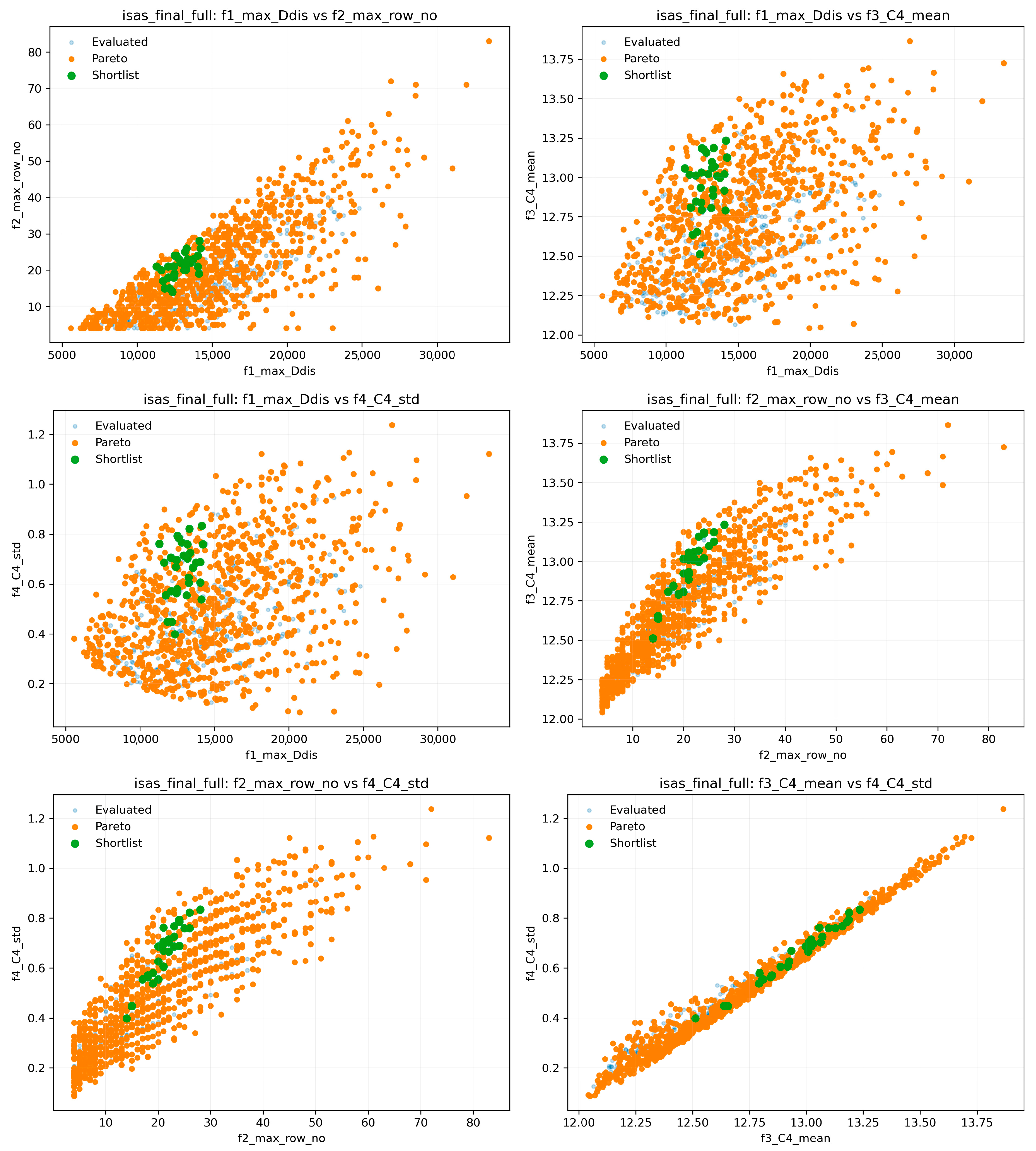
Figure A2.
Reduced-representation pairwise projections of evaluated Pareto set, shown for plot legibility when full front is visually dense. Panels match Figure A1: (a) f1–f2; (b) f1–f3; (c) f1–f4; (d) f2–f3; (e) f2–f4; (f) f3–f4; reduced set is used exclusively for visualization and does not change Pareto membership or any downstream decision calculations.
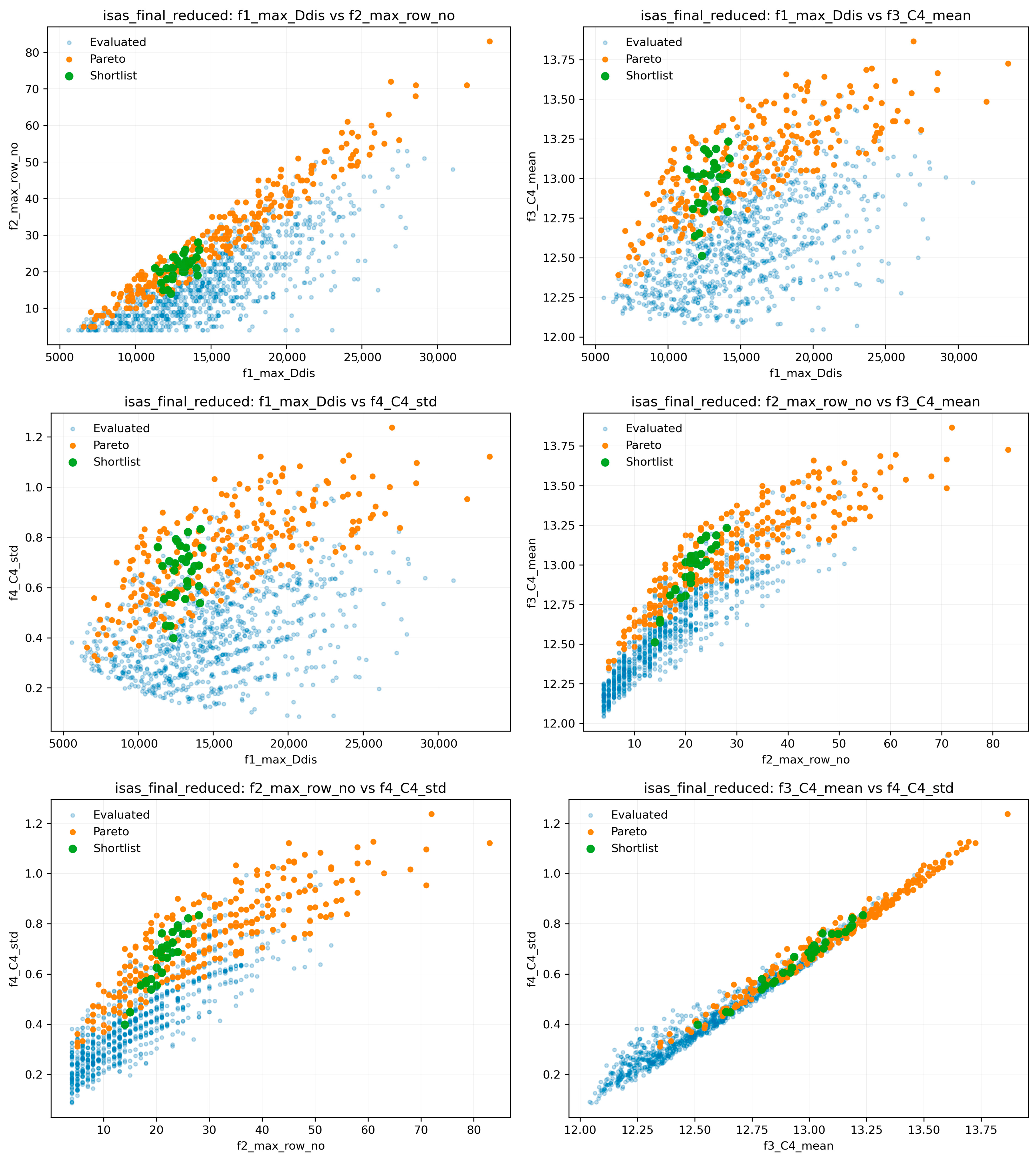
Appendix B
Table A9.
Learning-strategy alignment diagnostic (oracle acquisition score vs. Pareto membership).
Table A10.
Surrogate-family diagnostic (metrics in raw objective units).
Table A11.
Acquisition strategy comparison (same budget; post hoc oracle alignment).
| Algorithm A1. Stage SA verification (feature-drop ablation + rounding audits). |
| Throughout Algorithm A1, all settings of the baseline decision pipeline (Algorithm 2) are held fixed; Stage SA introduces no additional oracle evaluations and does not modify Input:
|
References
- Deb, K.; Pratap, A.; Agarwal, S.; Meyarivan, T. A fast and elitist multiobjective genetic algorithm: NSGA-II. IEEE Trans. Evol. Comput. 2002, 6, 182–197. [Google Scholar] [CrossRef] [Scilit]
- Zhou, A.; Qu, B.-Y.; Li, H.; Zhao, S.-Z.; Suganthan, P.N.; Zhang, Q. Multiobjective evolutionary algorithms: A survey of the state of the art. Swarm Evol. Comput. 2011, 1, 32–49. [Google Scholar] [CrossRef] [Scilit]
- Jin, Y. Surrogate-assisted evolutionary computation: Recent advances and future challenges. Swarm Evol. Comput. 2011, 1, 61–70. [Google Scholar] [CrossRef] [Scilit]
- Jones, D.R.; Schonlau, M.; Welch, W.J. Efficient global optimization of expensive black-box functions. J. Glob. Optim. 1998, 13, 455–492. [Google Scholar] [CrossRef] [Scilit]
- Forrester, A.I.J.; Keane, A.J. Recent advances in surrogate-based optimization. Prog. Aerosp. Sci. 2009, 45, 50–79. [Google Scholar] [CrossRef] [Scilit]
- Behzadian, M.; Otaghsara, S.K.; Yazdani, M.; Ignatius, J. A state-of-the-art survey of TOPSIS applications. Expert Syst. Appl. 2012, 39, 13051–13069. [Google Scholar] [CrossRef] [Scilit]
- Goldberg, D. What every computer scientist should know about floating-point arithmetic. ACM Comput. Surv. 1991, 23, 5–48. [Google Scholar] [CrossRef] [Scilit]
- Coello Coello, C.A. Theoretical and numerical constraint-handling techniques used with evolutionary algorithms: A survey of the state of the art. Comput. Methods Appl. Mech. Eng. 2002, 191, 1245–1287. [Google Scholar] [CrossRef] [Scilit]
- Miettinen, K. Nonlinear Multiobjective Optimization, 1st ed.; Springer: New York, NY, USA, 1998; Volume 12. [Google Scholar] [CrossRef] [Scilit]
- Elkhateeb, A.; Eldakdoky, S.; Fahmy, M.K.; Ibrahim, E. Sightline formulae in auditoria, review and new proposal to increase the visibility. Ain Shams Eng. J. 2024, 15, 102608. [Google Scholar] [CrossRef] [Scilit]
- Lawrence, A. Sightlines and soundlines—The design of an audience seating area. Appl. Acoust. 1983, 16, 427–440. [Google Scholar] [CrossRef] [Scilit]
- Joseph, D.; Kim, A.; Butler, A.; Haeusler, M.H. Optimisation for sport stadium designs: Advantages for shifting from macro level to micro level viewing optimisation in stadium design. In Proceedings of the CAADRIA 2015 (20th International Conference on Computer-Aided Architectural Design Research in Asia), Daegu, Republic of Korea, 20–22 May 2015; pp. 573–582. [Google Scholar] [CrossRef] [Scilit]
- Hudson, R.; Westlake, M. Simulating human visual experience in stadiums. In Proceedings of the SimAUD 2015 (Symposium on Simulation for Architecture and Urban Design), Alexandria, VA, USA, 12–15 April 2015. [Google Scholar]
- De Maesschalck, R.; Jouan-Rimbaud, D.; Massart, D.L. The Mahalanobis distance. Chemom. Intell. Lab. Syst. 2000, 50, 1–18. [Google Scholar] [CrossRef] [Scilit]
- Lloyd, S.P. Least squares quantization in PCM. IEEE Trans. Inf. Theory 1982, 28, 129–137. [Google Scholar] [CrossRef] [Scilit]
- Rousseeuw, P.J. Silhouettes: A graphical aid to the interpretation and validation of cluster analysis. J. Comput. Appl. Math. 1987, 20, 53–65. [Google Scholar] [CrossRef] [Scilit]
- Jin, Y. A comprehensive survey of fitness approximation in evolutionary computation. Soft Comput. 2005, 9, 3–12. [Google Scholar] [CrossRef] [Scilit]
- Knowles, J.D. ParEGO: A hybrid algorithm with on-line landscape approximation for expensive multiobjective optimization problems. IEEE Trans. Evol. Comput. 2006, 10, 50–66. [Google Scholar] [CrossRef] [Scilit]
- Forrester, A.I.J.; Sóbester, A.; Keane, A.J. Engineering Design via Surrogate Modelling: A Practical Guide; Wiley: Chichester, UK, 2008. [Google Scholar] [CrossRef] [Scilit]
- Jolliffe, I.T. Principal Component Analysis, 2nd ed.; Springer: New York, NY, USA, 2002. [Google Scholar] [CrossRef] [Scilit]
- Hornik, K.; Stinchcombe, M.; White, H. Multilayer feedforward networks are universal approximators. Neural Netw. 1989, 2, 359–366. [Google Scholar] [CrossRef] [Scilit]
- Kingma, D.P.; Ba, J. Adam: A Method for Stochastic Optimization. arXiv 2014, arXiv:1412.6980. [Google Scholar] [CrossRef] [Scilit]
- Deb, K.; Mohan, M.; Mishra, S. Towards a quick computation of well-spread Pareto-optimal solutions. In Evolutionary Multi-Criterion Optimization (EMO 2003); LNCS 2632; Springer: Berlin/Heidelberg, Germany, 2003; pp. 222–236. [Google Scholar] [CrossRef] [Scilit]
- Hwang, C.-L.; Yoon, K. Multiple Attribute Decision Making: Methods and Applications; Springer: Berlin/Heidelberg, Germany, 1981. [Google Scholar] [CrossRef] [Scilit]
- Sandve, G.K.; Nekrutenko, A.; Taylor, J.; Hovig, E. Ten simple rules for reproducible computational research. PLoS Comput. Biol. 2013, 9, e1003285. [Google Scholar] [CrossRef] [Scilit] [PubMed]
- Hamby, D.M. A review of techniques for parameter sensitivity analysis of environmental models. Environ. Monit. Assess. 1994, 32, 135–154. [Google Scholar] [CrossRef] [Scilit] [PubMed]
- Triantaphyllou, E.; Sánchez, A. A sensitivity analysis approach for some deterministic multi-criteria decision-making methods. Decis. Sci. 1997, 28, 151–194. [Google Scholar] [CrossRef] [Scilit]
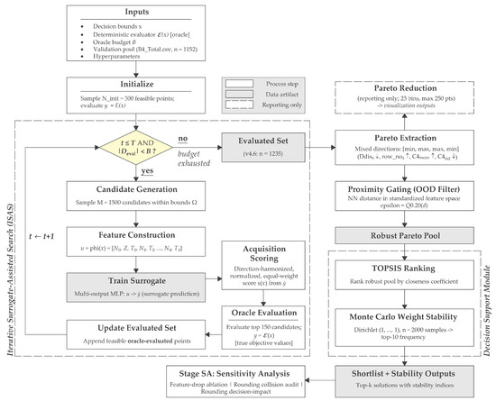
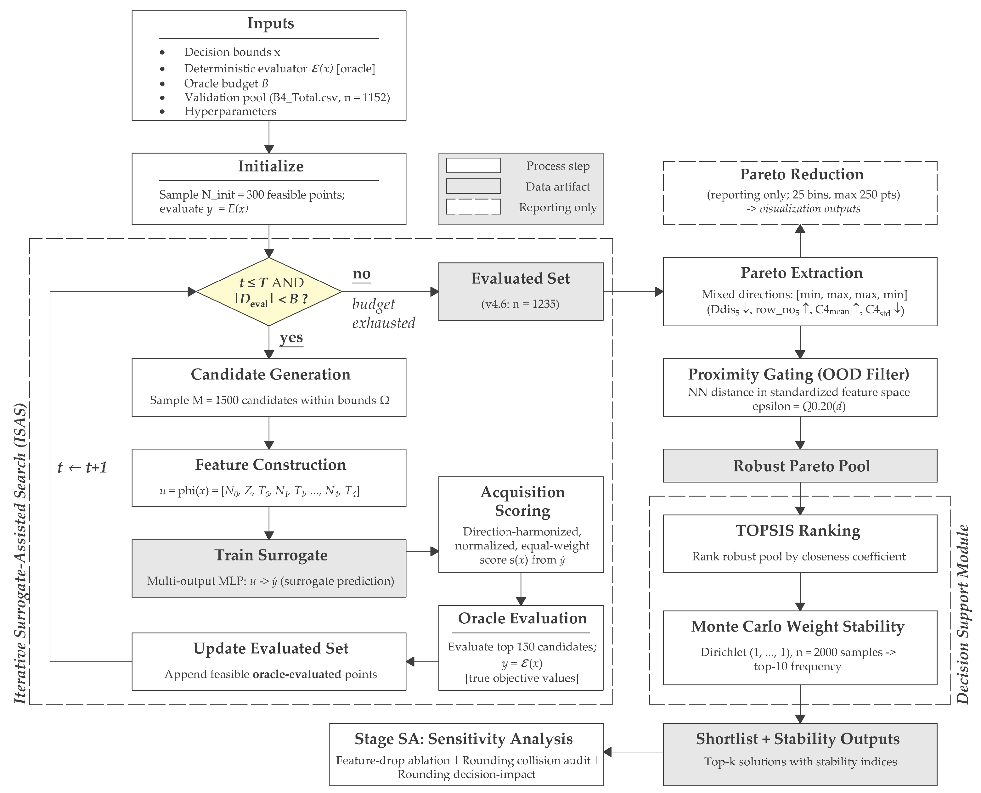
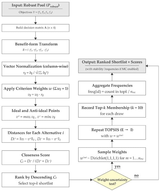
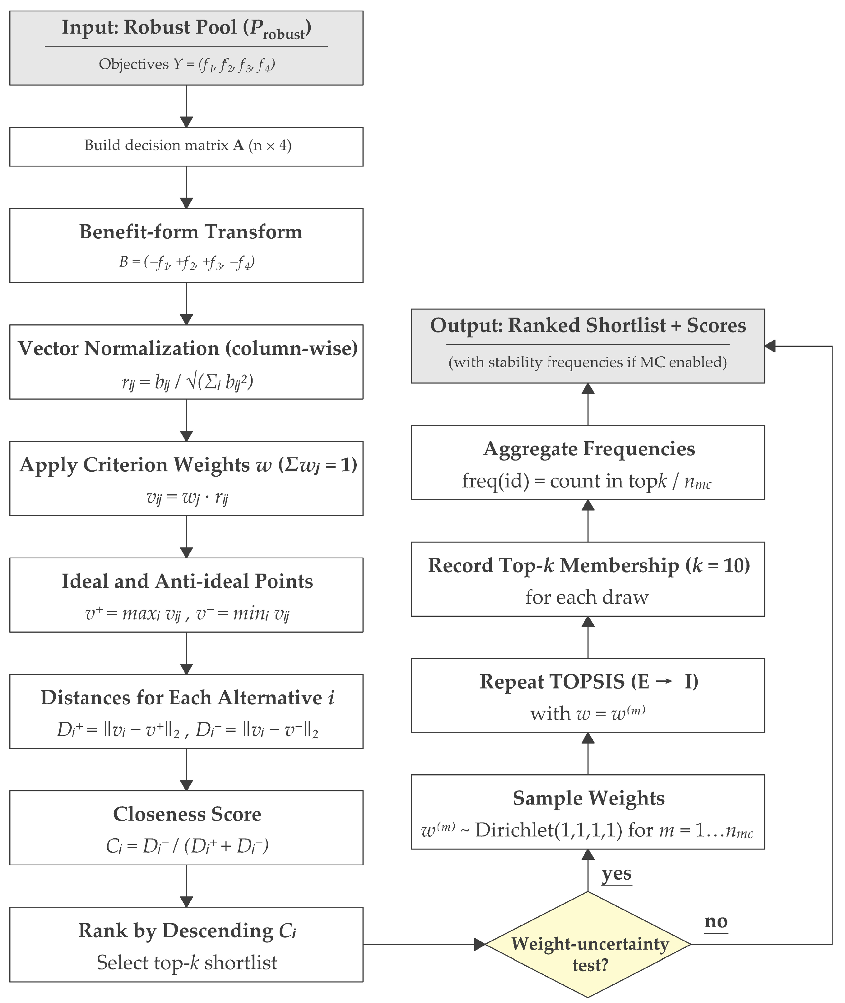
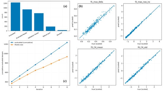
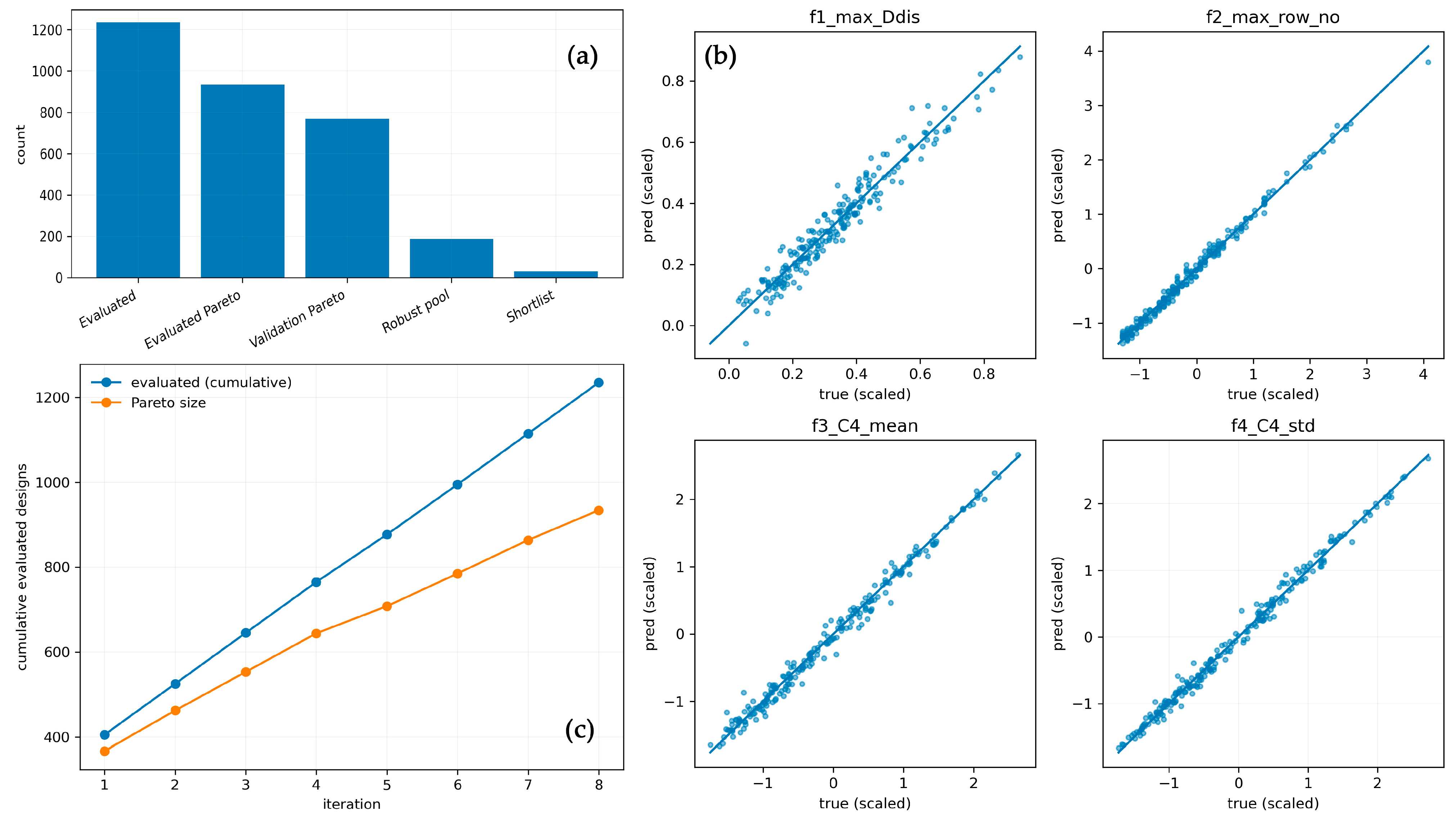
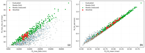
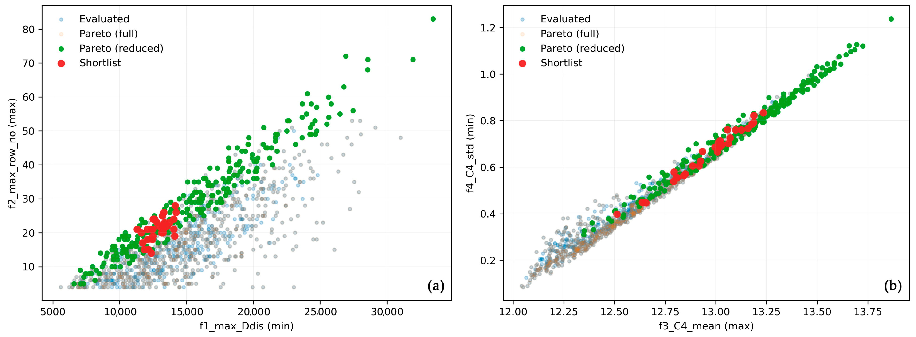
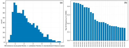
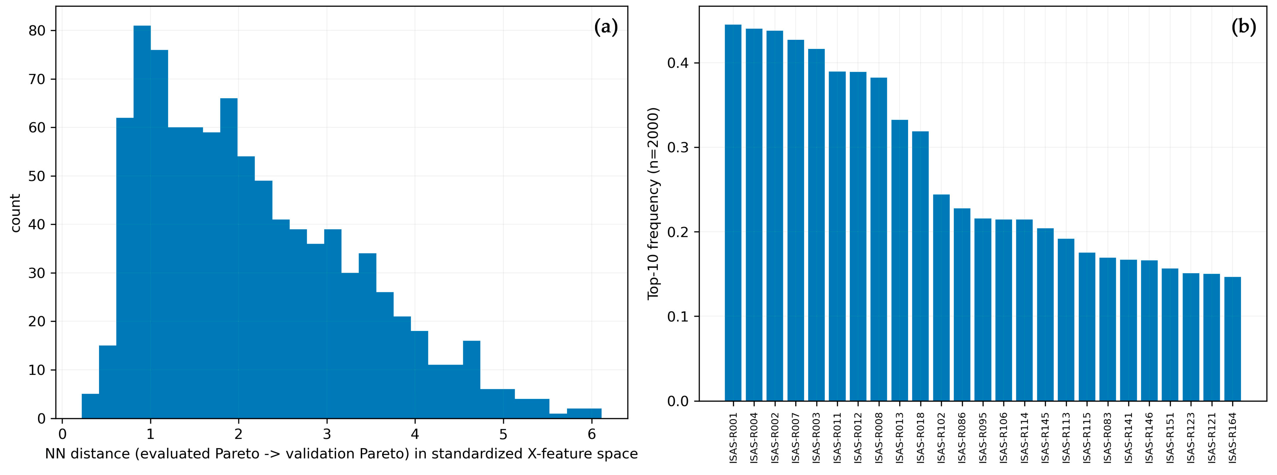
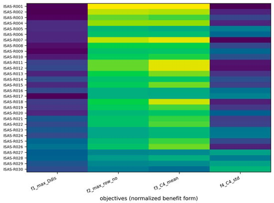
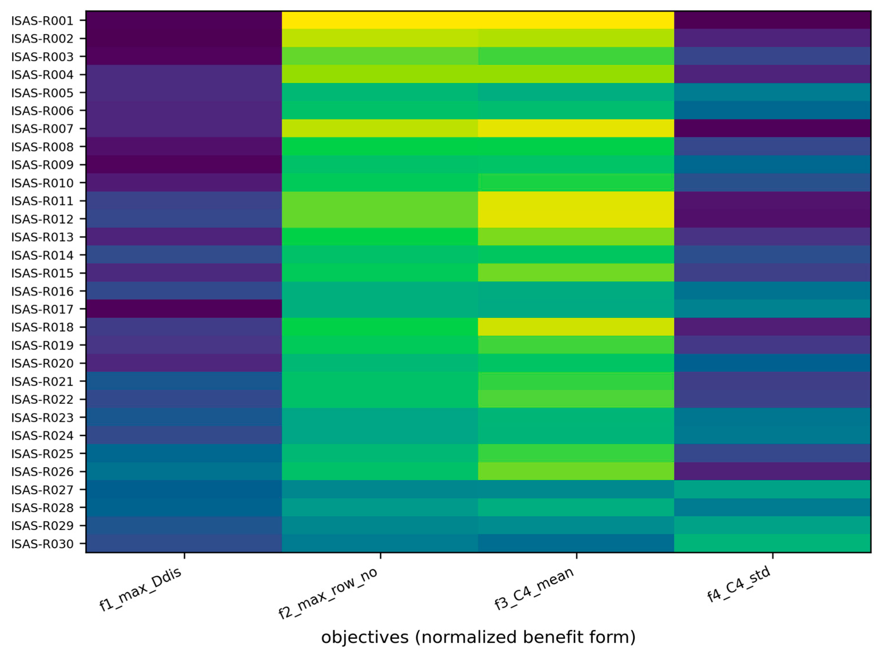
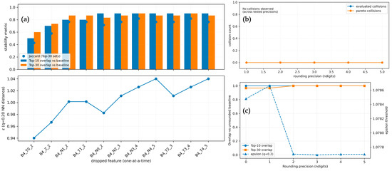
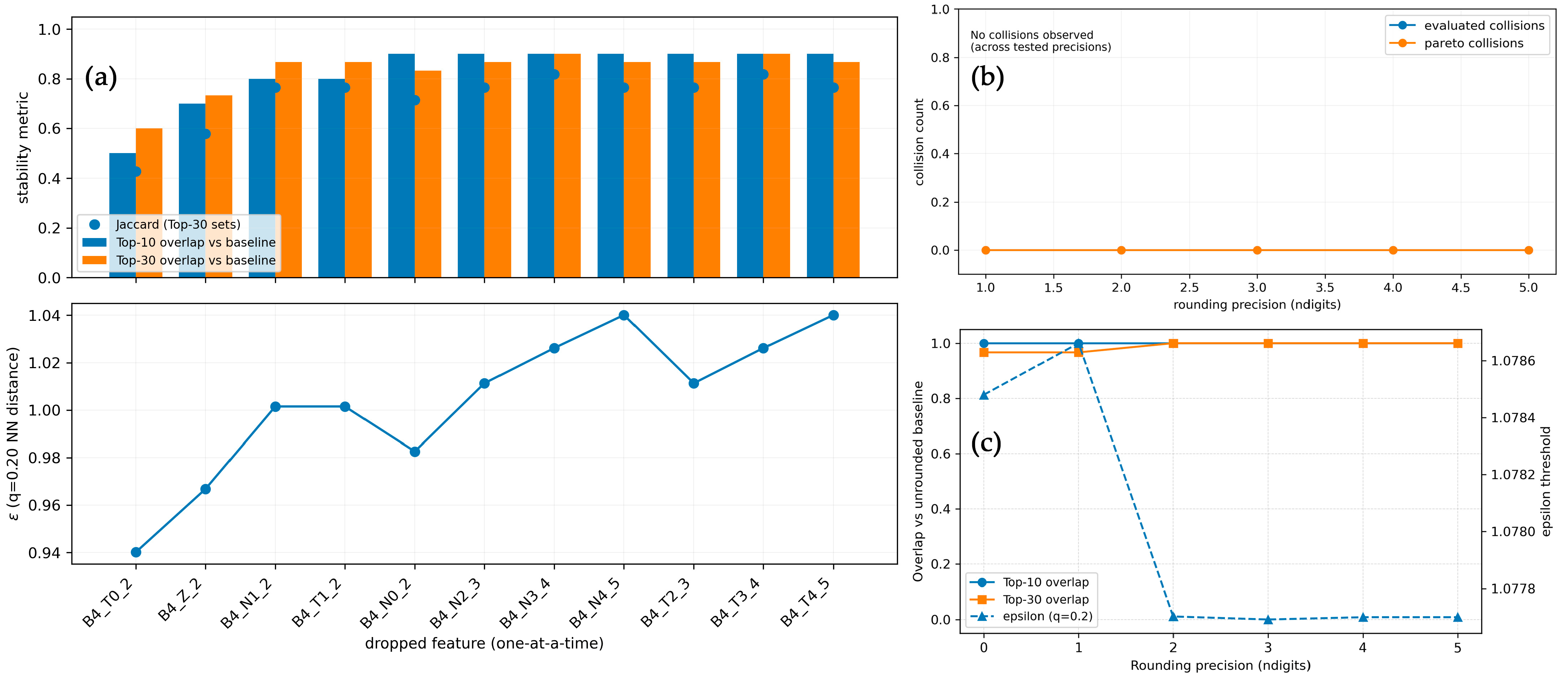

Disclaimer/Publisher’s Note: The statements, opinions and data contained in all publications are solely those of the individual author(s) and contributor(s) and not of MDPI and/or the editor(s). MDPI and/or the editor(s) disclaim responsibility for any injury to people or property resulting from any ideas, methods, instructions or products referred to in the content. |
© 2026 by the authors. Licensee MDPI, Basel, Switzerland. This article is an open access article distributed under the terms and conditions of the Creative Commons Attribution (CC BY) license.