


Abstract
In recent decades, considerable effort has been devoted to developing higher-order schemes for the discretization of convective terms that are both stable and reliable. In this work, the central idea is that the approximation should be made to reflect the physics of pure convection: the transported quantity is advected along streamlines, and information is propagated only in the upwind direction, i.e., the transported property is determined by previous values along the streamline but not by downstream values. In the proposed approach, streamlines on the computational mesh are represented by discrete streamlines, and the method is called the Discrete Streamline Method (DStreaM). A discrete streamline is constructed as a narrow triangle with one vertex at the node where the approximation is sought and two vertices at upstream neighbouring nodes. Discrete streamlines are oriented according to the local flow direction, in a manner similar to skew-upwind schemes, so that consistency with pure convection is ensured for DStreaM. The method is conservative only for uniform meshes with a constant velocity field; for general meshes and non-uniform velocity fields, it is non-conservative, and a non-zero local conservation error remains. The performance of DStreaM is assessed on the following standard test problems: convection of a step profile, a double-step profile, a sinusoidal profile, and the Smith–Hutton problem. DStreaM solutions are compared with those obtained using the first-order upwind scheme and second-order total variation diminishing (TVD) schemes with Minmod, QUICK, and SUPERBEE limiters. Across these benchmarks, high-resolution solution profiles and error levels comparable to those of the considered TVD schemes are produced by DStreaM. In the DStreaM construction, only local node coordinates and mesh connectivity are used; in this work, implementation is performed on both uniform Cartesian meshes and unstructured triangular meshes generated by a Delaunay triangulation. Representative results are reported with a focus on accuracy, iterative convergence, and conservation limitations.
Keywords:
Discrete Streamline Method (DStreaM); pure convection; skew-upwind scheme; convection-dominated flows; total variation diminishing (TVD) schemes; Smith–Hutton; unstructured triangular mesh MSC:
65M08; 76M12; 35L65; 65M12
1. Introduction
The development of higher-order approximation schemes for convective terms is an important problem in contemporary computational fluid dynamics (CFD). The Navier–Stokes (NS) equations are among the fundamental equations used in CFD to model fluid flows. The NS system describes the motion of viscous, incompressible or compressible, heat-conducting fluids and contains unsteady, convective, and diffusive terms. While these diffusive terms can usually be approximated in a straightforward way with at least second-order spatial accuracy, the convective terms are often discretized using the first-order upwind scheme. The first-order upwind scheme is very robust over a wide range of flow conditions, but it is excessively diffusive and, therefore, requires very fine meshes to obtain accurate solutions, which makes it computationally expensive in practice.
Second- and higher-order schemes for convective terms are widely available in modern CFD solvers and can provide substantially improved accuracy when applied carefully. Nevertheless, their use requires particular care near steep gradients and in convection-dominated regimes, where spurious oscillations and non-physical under- and overshoots may occur. From a theoretical point of view, Godunov’s theorem shows that no linear monotone scheme for a scalar conservation law can be more than first-order accurate; consequently, there is no simple modification of the first-order upwind scheme that yields a linear, monotone, higher-order discretization. This intrinsic limitation implies that schemes which are both accurate and robust must accept certain trade-offs (nonlinearity, loss of strict monotonicity, or other compromises), and it motivates the exploration of alternative viewpoints on the discretization of convection.
Up to now, two main routes have been followed in the development of higher-order approximation schemes for convective terms. One route is based on higher-order schemes that are essentially derived in one spatial dimension and then applied to multidimensional problems, primarily to reduce numerical diffusion. Total variation diminishing (TVD) schemes are typical representatives of this route: they are designed to prevent the undesirable oscillatory behaviour of higher-order schemes. In TVD schemes, the tendency towards oscillation is counteracted by adding an artificial diffusion contribution or by adding a weighting towards the upstream contribution. Early schemes based on these ideas were called flux-corrected transport (FCT) schemes; see Boris and Book [1,2]. Further contributions by van Leer [3,4,5,6], Harten [7,8], Sweby [9], Roe [10], Osher and Chakravarthy [11], Zijlema [12], Arora and Roe [13], Čada and Torrilhon [14], Ferreira et al. [15], Zhang et al. [16], Kriel [17], and many others have shaped the present-day family of TVD schemes.
More recent work has continued to refine such upwind-biased and high-resolution discretizations. Sukhinov et al. [18,19] and Dostál and Havlena [20] developed upwind-type schemes and mixed-mesh finite-volume methods tailored to transport-dominated hydrodynamics in complex geometries. High-order time-integration strategies for nonlinear convection–diffusion equations have also been investigated, for example, by Quinga et al. [21]. In the broader finite-volume context, Majima et al. [22] and Deng [23] introduced new TVD- and structure-preserving convection schemes that reduce numerical dissipation while maintaining stability, which have been implemented in open-source libraries.
The other route is based on multidimensional skew-upwind schemes that reduce numerical diffusion by taking into account the flow direction (in two and three dimensions) and selecting neighbouring points accordingly; in this sense, such schemes follow the streamlines. Raithby first presented the skew-upwind SUDS and SUWDS schemes in [24,25]. These schemes involve diagonal neighbours, as well as cells opposite to each cell face. Within the finite-volume context, Hassan, Rice, and Kim [26] proposed a mass-flow-weighted skew-upwind scheme as an improvement over the conventional skew-upwind scheme, which reduces numerical instability and numerical diffusion errors. In the finite-element context, Schneider and Raw [27] proposed an upwind procedure that accounts for the directionality of the flow field through a skewed approach while simultaneously precluding negative coefficients. Patel, Cross, and Markatos [28] retained the general objectives of Raithby’s scheme and proposed the CUPID scheme, which accounts for the flow angles at the corners of a cell rather than at the cell faces, as in Raithby’s SKEW schemes. A skew-upwind weighted differencing (SUWD) scheme was proposed by Busnaina, Zheng, and Sharif [29], where the convected quantity at a cell face is approximated by a weighted average of two quantities obtained by linear interpolation at two locations upstream of the resultant velocity vector at the cell face. Carey, Scanlon, and Fraser [30,31] developed the SUCCA scheme, which concentrates attention at the corners of finite-volume cells. Darwish and Moukalled [32] presented the STOIC scheme (Second- and Third-Order Interpolation for Convection), a high-resolution scheme developed within the normalized variable formulation of Leonard [33]. Ogedengbe and Naterer introduced the convective upwind scheme NISUS (Non-Inverted Skew-Upwind Scheme) in [34,35]; its main advantage is the avoidance of a costly inversion of the upwind coefficient matrix without a significant loss of accuracy. Karadimou and Markatos [36] retained the objectives of the CUPID and SUCCA schemes and reformulated the convection terms in the momentum and scalar conservation equations to treat three-dimensional flows, leading to the SUPER (Skew-Upwind and Corner Algorithm) scheme. Overall, both routes yield more accurate results than the first-order upwind scheme, but they may produce oscillations and under- or overshoots, especially in regions of strong gradients and in fast compressible flows. TVD schemes, in particular, perform very well for steady, slow, and moderate flows. Slow and moderate flows are often unsteady but close to a steady state for lower Reynolds numbers. For fast unsteady flows, TVD schemes may lose time accuracy [37], and for higher Reynolds numbers, even steady flows may exhibit unphysical oscillations. In such cases, a reliable solution can be obtained using the first-order upwind scheme, but only at the cost of substantial computational resources.
The spatial discretization of each term should, as far as possible, reflect the physical transport process that the term represents. Diffusive terms describe the exchange of a scalar quantity between neighbouring locations driven by its spatial gradients. The diffusive flux depends on the gradient of the concentration. Information is, therefore, exchanged in all directions around a given node. One of the simplest and most widely used approximations for diffusion terms is the central-difference scheme: it is formally second-order accurate in space and uses values at neighbouring nodes in all directions. In contrast, convection depends on the flow direction and is responsible for transporting the scalar quantity along streamlines. At the level of the continuous convection equation, the value of at a point is determined by the upstream data along the corresponding characteristic, which motivates discrete schemes that are predominantly upwind-biased along streamlines. Many TVD and related schemes, however, construct their nonlinear reconstructions from both upwind and downwind values of through limiter functions, in order to achieve higher-order accuracy while maintaining stability and avoiding spurious oscillations. In the present work, an alternative approach is explored in which the discrete stencil for the convective term is constructed solely from upstream nodes along a discrete streamline.
In this paper, an approximation approach for convective terms is presented that uses only upstream points and aligns the discrete stencil with the local streamline; it is thereby placed within the general class of skew-upwind schemes. The proposed Discrete Streamline Method (DStreaM) represents each discrete streamline by a narrow triangle with one vertex at the node where the flux is approximated and two vertices at upstream neighbouring nodes. The following four standard two-dimensional steady pure-convection test cases are used to assess the relative performance of DStreaM against standard schemes: the first-order upwind scheme and second-order TVD schemes with Minmod [10], QUICK [33], and SUPERBEE [10] limiters. Sweby [9] derived the necessary and sufficient conditions for a scheme to be second-order TVD; in this framework, the Minmod limiter traces the lower bound of the TVD region, SUPERBEE follows the upper bound, and QUICK lies in between.
The test problems considered are the convection of a step profile, a double-step profile, a sinusoidal profile, and the Smith–Hutton problem. Across these benchmarks, DStreaM produces solution profiles and error levels comparable to those obtained with the classical second-order TVD schemes considered. DStreaM is tested on a uniform Cartesian mesh and on an unstructured triangular (Delaunay) mesh, whereas the upwind and TVD schemes are evaluated on the uniform Cartesian mesh.
The present DStreaM formulation is strictly conservative only on a uniform Cartesian mesh with a constant velocity field. For general meshes and/or non-uniform velocities, the coefficient-compatibility residuals (Section 4.2) are, in general, non-zero; these residuals act as internal sources/sinks in the assembled global scheme and lead to a non-zero global conservation defect. The resulting global conservation error is quantified and discussed in Section 6.4, together with recommended use and limitations in Section 6.5. In its current form, DStreaM is best viewed as a high-resolution predictor/initial-guess scheme and as a prototype for future developments aimed at reducing and enforcing strict conservation on general meshes.
Supplementary Materials are provided, including the C++ source codes used in this work (ISO C++17; compiled with g++ 12.2.0 on Debian GNU/Linux 12), the supporting datasets, MATLAB 2020b, Python 3.12.9, Bash post-processing scripts (GNU bash 5.2.15), and Wolfram Mathematica 14.0 (.nb) notebooks containing the derivations of the governing equations.
2. Physical Considerations on Diffusion and Convection
Here, more detailed considerations of pure convection and pure diffusion are presented, which are important for the formulation and interpretation of the proposed approximation approach.
The steady convection–diffusion equation for a general property can be written in the form
where u and v are the velocity components along the x- and y-axes, is the density, and is a (constant) diffusion coefficient.
The diffusive terms in (1) describe pure diffusion. Diffusion is the movement of molecules or atoms from regions of high concentration (or high chemical potential) to regions of low concentration, driven by spatial gradients of . For isotropic diffusion with constant , the diffusive flux depends on the gradient of the concentration and is independent of the velocity field, so information is effectively exchanged in all directions around a given point. One of the simplest and most widely used discretizations for diffusion terms is the central-difference scheme: it is formally second-order accurate in space and uses values at neighbouring nodes in all directions. On uniform orthogonal grids, the central-difference approximation is consistent with the isotropic character of the diffusion operator and does not introduce spurious oscillations for pure diffusion problems. Therefore, a diffusion discretization based on a symmetric stencil is naturally aligned with the underlying physics of the diffusive process.
In contrast, convection is responsible for the transport of the scalar quantity by the flow and depends on the direction of the velocity field. For the continuous convection equation, the value of at a point is determined by the upstream data along the corresponding characteristic, which can be visualized as an information propagation cone. Figure 1b illustrates this schematically: information about at a given point is available only from within the upstream cone, while regions outside this cone, including directions opposite or normal to the velocity, do not influence the local value of in the absence of diffusion. This motivates discrete schemes for the convective terms that are predominantly upwind-biased along streamlines and whose stencils reflect the directional nature of advective information propagation.
Figure 1.
Schematic information propagation in a diffusion-dominated problem (a) and a convection-dominated problem (b).
The convective terms in Equation (1) represent the convection of the scalar by the velocity field. In the absence of diffusion and sources, convection can be idealized as the motion of fluid particles through streamtubes without exchange of the transported property between neighbouring streamtubes. The transported quantity is , and the velocities in the convective terms can be interpreted as determining the geometry of streamlines or pathlines of the fluid particles; see, for example, the derivation and discussion of the Navier–Stokes equations in [38,39]. Figure 2 illustrates the motion of a fluid particle from time to time through a streamtube. The velocity field is assumed known at each position, but, for pure convection, the value of the transported property at time is determined solely by its values at earlier times along the trajectory, up to ; it does not depend on future values such as at , which have not yet occurred and are not represented in the convective terms. This one-way (upstream-to-downstream) propagation of information in time and along streamlines is the key characteristic of pure convection. In the absence of diffusion and sources, the transported quantity of a given fluid particle remains constant along its path,
For constant density, this reduces to
Thus, for a steady pure-convection problem, the solution can be obtained by tracing characteristics (streamlines or pathlines) from the inflow boundary to each point in the domain. The basic idea of the proposed approach is to build a discrete approximation that reflects this unidirectional transport of information along streamlines.
Figure 2.
Transport of a fluid particle through a streamtube.
The propagation of information in convection-dominated problems on a mesh is important for designing an approximation that corresponds to the modelled flow. Figure 3 shows schematic information-propagation cones associated with the convective terms at the nodes of a uniform Cartesian mesh. In the ideal pure-convection limit, each cone half-angle (see Figure 1b) tends to zero (); the cone degenerates into a curve aligned with the streamline, and the value at a node is equal to the value at the upstream intersection of this curve with either another node or the inflow boundary of the computational domain. The limit corresponds to a numerical scheme without cross-stream numerical diffusion (often called false diffusion), i.e., without artificial spreading of information normal to the streamline. In practical discrete schemes for pure convection, numerical diffusion leads to a finite cone angle , as sketched in Figure 3.
Figure 3.
Information-propagation cones of a convection-dominated problem at mesh nodes.
The cones in Figure 3 can be grouped according to whether they intersect the node . In the example shown, the first group consists of nodes whose information certainly reaches ; these are and . A second group consists of nodes whose cones may or may not intersect , depending on the cone angle ; in the figure, these are , , , and . In the particular case illustrated, information from node reaches , while information from nodes , , and does not. The remaining nodes, , , , , and , form a third group whose information does not reach in this convection-dominated picture. The information-propagation cone associated with can also be considered in the reversed sense (rotated by ), which identifies the nodes that can be influenced by ; see Figure 4. In the present DStreaM formulation, the discrete stencil for the convective term at node is constructed from nodes belonging to the upstream domain of dependence of , i.e., from those nodes whose information can reach according to this cone-based interpretation.
Figure 4.
Reversed information-propagation cone and corresponding shape function for the convective term; the triangle is a discrete representation of a streamline through node .
3. Discrete Streamline Method (DStreaM)
3.1. Model Problem and Notation
A two-dimensional problem is considered here; the extension of DStreaM to three dimensions is straightforward.
The pure-convection equation is obtained from the convection–diffusion Equation (1) by setting . For simplicity, a constant density is assumed (), which leads to
Since is constant, it can be factored out of the divergence operator and divided out of the equation.
3.2. Discrete Streamlines and Triangular Stencil
For clarity, DStreaM is first introduced on a uniform Cartesian mesh. The construction relies only on local node coordinates and connectivity; therefore, the same discrete-streamline triangle can be built on unstructured meshes by selecting two appropriate upstream neighbours from the local connectivity graph. Figure 4 illustrates the reversed information-propagation cone for node . In the configuration shown, information from , , and can reach . The nodes , , and lie on a straight line, and the information that actually propagates to along this line comes from the closest upstream node ; the more distant node is “shadowed” by along the same streamline. Therefore, the shape function is chosen to interpolate the three nodes , , and , as shown in Figure 4. In this formulation, the shape function for the convective term is associated with a triangle with vertices at , , and . This triangle is interpreted as a discrete representation of the streamline through and forms the basic building block of the proposed approach, which motivates the name Discrete Streamline Method. The shape function is taken to be linear,
where the coefficients , , and are chosen such that interpolates the nodal values at the three vertices of the triangle.
3.3. Shape Function and Nodal Reconstruction
To obtain a more general expression, the three nodes of the shape function are denoted by , , and (Figure 5a), corresponding to , , and in Figure 4, respectively. The coefficients , , and of the linear shape function (3) are determined by requiring that interpolates the nodal values at the three vertices with coordinates , , and ,
Solving this linear system yields
Figure 5.
Averaging schemes: shape function with average velocities (a), horizontal average velocity approximation (b), and vectors and used to determine the sector of the approximation scheme (c).
The velocity is approximated locally by an average value over the three nodes,
which is used as a constant approximation of the velocity within the upwind triangle associated with the shape function.
3.4. Final Discrete Scheme and Algorithm
Figure 5b shows a geometric representation of . In the present formulation, the upwind triangular region coincides with the triangular region of the shape function. The average velocities and are treated as constant over this upwind triangle. Substituting the shape function (3) and the average velocities (5) into the convection Equation (2) and integration over the triangular region yields
where V is the area of the upwind triangle and the derivatives of the linear shape function are constant over the triangle. Eliminating and using (4) and simplifying yields a nodal relation of the form
with coefficients
A detailed derivation of the nodal relation (7) using barycentric (area) coordinates on the triangular control volume is given in Appendix A. The full derivation is also available in the Supplementary Materials as a Wolfram Mathematica .nb notebook and its PDF export:
- Simple_Conv_equation_derive_General_with_Barycentric_coordinates_and_constant_velocities_ua_va.nb
- Simple_Conv_equation_derive_General_with_Barycentric_coordinates_and_constant_velocities_ua_va.pdf
Thus, the value at the central node is expressed as a convex combination of the values at two upstream nodes and , with weights that depend on the local average velocity and the geometry of the triangular stencil.
3.4.1. Upwind-Triangle Selection on a Uniform Cartesian Mesh
On a uniform Cartesian mesh, the stencil radius R is defined as the half-width of the neighbourhood around node . Thus, corresponds to a stencil, to a stencil, and so on; see Figure 6. On a uniform Cartesian mesh with a spatial step
the nodes considered for the approximation at lie within the square
Figure 6.
Triangular shape functions on a Cartesian mesh, centred at node for stencil radii (a), (b), and (c).
Figure 6 shows the triangular shape functions associated with stencil radii , , and for node . Each triangle can be interpreted as a candidate discrete streamline through for the given radius. For , the neighbours involved have indices and , and the shape functions partition the plane around into eight sectors. When R is increased by one, each existing sector is subdivided and additional nodes are included, as follows: the numbers of candidate triangles for , , and are 8, 16, and 32, respectively (see Figure 6). For , all angles at vertex are equal, whereas for larger radii, the sectors generally have different angles.
For each node, the sector and the corresponding upstream nodes and used in the approximation are selected according to the local flow direction. For a given stencil radius R, the neighbours of are grouped into sectors, with each sector being associated with a candidate upwind triangle whose vertices are ; see Figure 5. For each candidate triangle, a sector-averaged velocity is computed using the same averaging formula as in (5). Candidates for which falls below a small tolerance are discarded.
The median vector is then defined
which points from the midpoint of the edge towards the central node , and evaluated as the signed squared cosine
This quantity is equal to sign(cosθ) cos2θ, where is the angle between and . Among all candidate sectors, the one with the largest value of is selected. In this way, the chosen upwind triangle is the one whose median direction is best aligned with the local flow and for which the flow points from the upstream edge towards the central node . The corresponding triangle is then used as the discrete streamline for DStreaM.
As the stencil radius R increases, the discrete streamline becomes narrower and tends to a line segment; in regions where the velocity field is locally uniform, this leads to a closer alignment with the exact streamline. When the local velocity field varies strongly, however, very large values of R may produce discrete streamlines that deviate significantly from the true local characteristics, and smaller radii are preferable. For non-uniform velocity fields, the average velocity depends on the selected sector and must be recomputed for each candidate triangle in the selection algorithm.
The above selection algorithm is implemented as part of the full DStreaM C++ code provided in the Supplementary Materials; for implementation details, see folder DStreaM_code (Cartesian mesh).
3.4.2. Upwind-Triangle Selection on Unstructured Meshes
Figure 7 shows an unstructured mesh and the corresponding upwind triangles for stencil radii and around the node . At a node (unknown ), an upwind triangle is formed by selecting two upstream neighbours and (values and ), such that acts as the discrete streamline control volume. For a prescribed stencil radius R, a candidate set is built by a breadth-first expansion of the mesh connectivity graph by R layers (an R-ring neighbourhood). Sector construction and shadowing removal are then performed geometrically using node coordinates, as illustrated in Figure 7d–g.
Figure 7.
Unstructured triangular mesh (green) (a); DStreaM discrete-streamline triangles (grey, black edges) constructed around node for stencil radii (b) and (c); candidate neighbour nodes in the local coordinate system (d) mapped to local polar coordinates (e); angular sorting and removal of shadowed nodes (f); and selection of the upwind triangle based on (g).
Algorithm (Upwind-Triangle Selection on an Unstructured Mesh)
- 1.
- Neighbourhood construction. Construct the candidate node set within stencil radius R (e.g., by breadth-first expansion of the connectivity graph); see Figure 7d.
- 2.
- Relative vectors and angles. For each , form the local coordinates and compute the local polar coordinateswhere primes (′) denote local coordinates relative to ; see Figure 7e.
- 3.
- Angular sorting. Sort the candidates by ; see Figure 7f.
- 4.
- Shadow removal. If two nodes have nearly the same direction from , i.e., (with periodic wrap-around), retain only the closer one (smaller r), and obtain a list of nodes between which upwind triangles are formed, where seconds (″) denote sorted local coordinates; see Figure 7f.
- 5.
- Candidate triangles. Let the remaining nodes in angular order be . Form M candidate triangles with wrap-around ; see Figure 7g.
- 6.
- Upwind selection. For each , compute the triangle-averaged velocity (as in (5), using the three vertices of ). Discard candidates with . Select the triangle maximizing , with and defined as in Section 3.4 and Equations (11) and (12). Assign its two non-central vertices as and ; see Figure 7g.
The selected upwind triangle is then used to evaluate from (7) with either the unlimited coefficients (8) or the limited coefficients (13).
The above selection algorithm is implemented as part of the full DStreaM C++ code for unstructured meshes provided in the Supplementary Materials; for implementation details, see folder DStreaM_code_unstuctured_mesh (unstructured triangular mesh).
3.4.3. Limiter for Coefficients and Monotonicity
The proposed approximation corresponds locally to a straight streamline, which makes the method simple, but also introduces limitations when the velocity field is strongly non-uniform and the stencil radius is large. In the numerical experiments with uniform velocity fields—the convection of a step profile, a double-step profile, and a sinusoidal profile—DStreaM produces solutions without under- or overshoots even for relatively large radii. When local streamlines are curved, however, the approximation shows its limitations for large R. The Smith–Hutton problem, in which the streamlines are strongly curved (see Section 5.4), provides a representative example. For this test case, DStreaM yields bounded solutions without under- or overshoots for radii up to . For , under- and overshoots appear in the solution.
A standard approach to prevent under- and overshoots and to enhance convergence is to enforce positivity of the coefficients and in (7); see, for example, the recommendations by Patel, Cross, and Markatos [28]. In the present context, this leads to the following limiter:
With this definition, , and the weights and in (7) are always non-negative and sum to one. Consequently, lies between and , which prevents new extrema from being created at the node.
The effect of limiting is illustrated in Figure 13, which compares solutions obtained with the unlimited coefficients (8), panels (a)–(e), and with the limited coefficients (13), panels (g)–(k). For radii up to , both formulations give essentially identical results. Differences appear for . For , the unlimited scheme exhibits small under- and overshoots, whereas the limited scheme produces a solution without under- or overshoots (Figure 13e and Figure 13j, respectively). For , the unlimited scheme develops large under- and overshoots (Figure 13e), while the limited scheme avoids overshoots but introduces some non-physical jumps between neighbouring nodes (Figure 13k). For the spatial resolution considered here, the maximal stencil radius that yields physically realistic results with the limited coefficients is . Overall, the limiter increases the robustness of the scheme and extends the range of stencil radii for which acceptable solutions are obtained.
Because the shape function and the coefficients in (7) depend only on the coordinates of three nodes and the local average velocity, the same discrete-streamline construction is used on unstructured meshes by selecting two upstream neighbours from the local connectivity graph (algorithms described in Section 3.4.1 and Section 3.4.2).
In summary, the DStreaM algorithm at a given node consists of the following steps:
- 1.
- Compute the local average velocities and using (5).
- 2.
- Determine the upwind nodes and by selecting the appropriate triangular sector for the chosen stencil radius R.
- 3.
4. Conservation Properties of DStreaM
Conservation is a fundamental requirement for numerical schemes that approximate transport equations. In a conservative formulation, the discrete convective operator can be written as a balance of numerical fluxes across interfaces, so that contributions associated with internal nodes (or internal faces) cancel when the equations are summed over the domain, and only boundary contributions remain.
In the present DStreaM formulation, the discrete relation at a node is obtained by integrating the convection equation over an upwind triangular region and expressing the central value in terms of two upstream values and ,
where the coefficients , , and are given by (8) in terms of the local geometry and the average velocity in the upwind triangle. In this section, the conditions under which the global scheme is conservative are examined.
4.1. Uniform Cartesian Grid with Constant Velocity
The idealised case of a uniform Cartesian grid with mesh spacing and a strictly positive constant velocity field is first considered
For this configuration, the upwind triangles associated with interior nodes have the same shape up to translation, and the average velocity in each triangle coincides with the constant velocity,
Figure 8 illustrates the upwind triangle associated with node (denoted as upwind triangle 0) and the upwind triangles of its neighbours that share the nodes , , and . In this configuration, the following are observed:
Figure 8.
Upwind triangle associated with node (upwind triangle 0) and upwind triangles of its neighbouring nodes that share the vertices , , and .
- Upwind triangle 0 has a central value at and upstream vertices at and at ;
- Upwind triangles 1 and 2 have centred values at node and at node and are downwind of ;
- Upwind triangles 3 and 4 have centred values at and at and are lateral neighbours;
- Upwind triangles 5 and 6 have centred values at and at and are upstream neighbours.
All of these triangles involve at least one of the nodes , , and as vertices (see Figure 8).
For a generic upwind triangle k, the coefficients in the local DStreaM relation (14) are denoted by and , and is set to . Thus, for triangle k, the following holds:
Conservation requires that when the relations (15) are summed over all upwind triangles that share a given interior node, the contributions associated with that node cancel. For the configuration in Figure 8, cancellation of the three interior nodes , , and leads to the following compatibility conditions for the coefficients:
Equation (16) expresses the requirement that the contributions involving cancel when the equations for upwind triangles 0, 1, and 2 are added; Relations (17) and (18) express the analogous conditions for and when triangles 0, 3, 5 and triangles 0, 4, 6 are combined, respectively.
On the uniform Cartesian grid with constant velocity, all these upwind triangles have identical geometry and the same average velocity. Using the expressions in (8) for and , one obtains for each triangle
so that
for all k. Substituting these expressions into (16)–(18) shows that all three compatibility conditions are satisfied identically, e.g.,
Therefore, for a uniform Cartesian mesh and a constant velocity field, the DStreaM discretization is conservative: when the local relations (15) are summed over all upwind triangles, the contributions associated with interior nodes cancel, and only boundary contributions remain.
4.2. Non-Uniform Velocity and General Meshes
In the general case of non-uniform velocity fields or non-uniform meshes, the situation changes. For a generic upwind triangle with vertices corresponding to nodes 0, 1, and 2, the average velocity entering the DStreaM coefficients is computed as
so that the coefficients and in (8) depend on both the local geometry and the local variation of the velocity field. As a consequence, the coefficients and associated with different upwind triangles sharing a given node are no longer identical, even when the underlying mesh is uniform.
For example, consider again the configuration in Figure 8 and the compatibility condition (16) for the node , which, in the conservative uniform case, reads
It is convenient to define a local conservation residual at as
Non-zero represents a failure of the coefficient-compatibility condition required for internal cancellation between neighbouring upwind triangles. When the nodal relations are assembled over the whole mesh, these non-cancelling contributions appear as a spurious internal production/consumption term (source/sink) in the global algebraic balance, and, therefore, can generate a net boundary–flux imbalance even after full iterative convergence.
In the uniform Cartesian constant-velocity case, the coefficients in all involved triangles are identical and (16) holds exactly, so . For non-uniform velocity fields and/or non-uniform meshes, the coefficients and vary from triangle to triangle, and in general, . Analogous residuals and can be defined for the nodes and based on the compatibility relations in (17) and (18). These non-zero local residuals are the origin of the discrete conservation error of the global scheme.
Further development will focus on reducing local residuals (enforcing coefficient compatibility more strictly), with the aim of improving global conservation on general meshes and for non-uniform velocity fields.
Consequently, the present DStreaM formulation is strictly conservative only in the special case of a uniform Cartesian mesh with a constant velocity field. This covers the first three test problems with constant convection velocity; in those cases, it has been verified that the discrete conservation error is at the level of machine precision for all grid resolutions considered. For the Smith–Hutton problem, which involves a non-uniform velocity field, the compatibility relations in (16)–(18) are no longer satisfied and DStreaM exhibits a non-zero global conservation error. In the present computations, this error is typically in the range – (see results in Section 5.4), whereas the finite-volume reference discretisation preserves the transported quantity to about . Although the DStreaM errors remain small in absolute terms and do not visibly affect the solution quality in the present benchmarks, they confirm that the current formulation is not strictly conservative. Therefore, the development of fully conservative streamline-based variants of DStreaM remains an important topic for future work.
5. Test Problems and Numerical Results
DStreaM is tested on the following four standard steady pure-convection benchmark problems: convection of a step profile, convection of a double-step profile, convection of a sinusoidal profile, and the Smith–Hutton problem. All discrete systems are solved using a pointwise Gauss–Seidel iteration with an initial guess . The order in which mesh nodes are updated influences the number of iterations required for convergence. Two update strategies are used. For the TVD schemes, each iteration starts from the corner . For the first-order upwind scheme, DStreaM, and DStreaM (U), the starting corner is cycled between the four corners of the domain from one iteration to the next. This ordering is used to reduce iteration-order bias; however, the consistently low iteration count mainly follows from the strictly upstream dependence of the discrete operator, which makes each iteration close to a marching update along the convection direction.
Convergence is monitored using the maximum change in between two successive Gauss–Seidel iterations,
and all runs are terminated when
In the tables below, this quantity is reported in the column labelled “Max change”.
The following schemes are compared: the first-order upwind scheme; DStreaM with stencil radii (denoted as DStreaM R1 to R5); DStreaM on an unstructured mesh with stencil radii (denoted as DStreaM R1 (U) to DStreaM R5 (U)); and TVD schemes with Minmod, QUICK, and SUPERBEE limiters. For the TVD schemes, under-relaxation is employed and the under-relaxation factor is tuned so as to minimise the number of iterations needed to reach the prescribed convergence criterion.
DStreaM can reproduce the exact discrete solution (i.e., the exact solution of the discrete pure-convection problem on the given mesh) for a uniform velocity field when the stencil radius is sufficiently large. For the test problems with uniform velocity, if the horizontal and vertical components are equal (), DStreaM already obtains the exact solution for radius . These include the convection of a step profile, a double-step profile, and a sinusoidal profile. To avoid this trivial situation and obtain a more discriminating test, and are used in these cases.
All results for the upwind and TVD schemes are obtained on a uniform Cartesian mesh.
Results labelled as DStreaM Rk are obtained on uniform Cartesian meshes (Figure 6), whereas DStreaM Rk (U) denotes the unstructured triangular-mesh implementation (Figure 7). Unstructured meshes (triangulations) are generated in Gmsh using the built-in 2D Delaunay algorithm [40]. Mesh generation is performed programmatically via the Gmsh C++ API integrated into the solver.
- Error norms and observed convergence rate.
The test problems considered in this section are steady pure-convection problems with a prescribed velocity field. The reference solution is obtained from the method of characteristics; for steady problems, characteristics coincide with streamlines of the velocity field (i.e., by mapping the inlet profile along streamlines of the prescribed velocity field). The discrete error at node I is
where is the node location and N is the number of degrees of freedom (number of nodes in the mesh). The following area-weighted discrete norms are used:
where is the area associated with node I (so that equals the domain area in 2D).
For uniform Cartesian meshes used here (), the characteristic mesh size is taken as . On unstructured meshes, h denotes the characteristic element size used in the mesh generator (Gmsh).
For two meshes with sizes and , the observed order in a given norm is
Computing environment and timing.
All computations were performed on a desktop workstation running Debian 12 (bookworm), equipped with an Intel Core i5-9400F CPU (2.90 GHz) and 64 GB RAM. The code was compiled with g++ using -O2 -mavx2. Reported compute time is the wall-clock time measured inside the iterative solver loop only (excluding mesh generation, memory allocation, and initialization). Timings were obtained from 20 repeated executions and are reported as the median value.
All source codes, supporting datasets, and post-processing scripts used to generate the results reported in this study are provided in the Supplementary Materials, including the DStreaM C++ codes for structured Cartesian and unstructured meshes (DStreaM_code and DStreaM_code_unstuctured_mesh) and the reference TVD C++ implementation (2D_convection_problem_TVD_code).
5.1. Convection of a Step Profile
For the convection of a step profile, and are used. The boundary conditions are the standard ones for this problem, see Figure 9a. The mesh is a uniform Cartesian grid with nodes. Figure 9b shows the profiles at obtained with considered schemes.
Figure 9.
Convection of a step profile: (a) physical domain, (b) profiles at obtained with the different schemes, and (c) and (d) error norms.
Figure 9c,d report the and error norms versus mesh size h on log–log axes. The corresponding observed rates and are summarised in Table 1.
Supporting datasets and post-processing scripts used to generate the results of the step profile are provided in the Supplementary Materials in the following folders:
- Convection_of_a_step_profile_problem_DStreaM
- Convection_of_a_step_profile_problem_DStreaM_unstructured
- Convection_of_a_step_profile_problem_TVD
- Convection_of_a_step_profile_problem_DStreaM_mesh_convergence_L1_L2_log-log_plot_data
- Convection_of_a_step_profile_problem_DStreaM_unstructured_mesh_convergence_L1_L2_log-log_plot_data
- Convection_of_a_step_profile_problem_TVD_mesh_convergence_L1_L2_log-log_plot_data
5.2. Convection of a Double-Step Profile
For the convection of a double-step profile, and are again used. The boundary conditions are the standard ones for this problem, see Figure 10a. The mesh is a uniform Cartesian grid with nodes. Figure 10b shows the profiles at obtained with the considered schemes.
Figure 10.
Convection of a double-step profile: (a) physical domain, (b) profiles at obtained with the different schemes, and (c) and (d) error norms.
Figure 10c,d report the and error norms versus mesh size h on log–log axes. The corresponding observed rates and are summarised in Table 2.
Table 2.
Iterative performance on the mesh and observed convergence rates for the convection of a double-step profile shown in Figure 10, with convergence criterion . The observed orders and are obtained from a least-squares fit of on the four finest meshes used in the mesh-refinement study (Figure 10c,d).
Supporting datasets and post-processing scripts used to generate the results of the double-step profile are provided in the Supplementary Materials in the following folders:
- Convection_of_a_double_step_profile_problem_DStreaM
- Convection_of_a_double_step_profile_problem_DStreaM_unstructured
- Convection_of_a_double_step_profile_problem_TVD
- Convection_of_a_double_step_profile_problem_DStreaM_mesh_convergence_L1_L2_log-log_plot_data
- Convection_of_a_double_step_profile_problem_DStreaM_unstructured_mesh_convergence_L1_L2_log-log_plot_data
- Convection_of_a_double_step_profile_problem_TVD_mesh_convergence_L1_L2_log-log_plot_data
5.3. Convection of a Sinusoidal Profile
For the convection of a sinusoidal profile, and are again used. The boundary conditions are the standard ones for this problem, see Figure 11a. The mesh is a uniform Cartesian grid with nodes. Figure 11b shows the profiles at obtained with the considered schemes.
Figure 11.
Convection of a sinusoidal profile: (a) physical domain, (b) profiles at obtained with the different schemes, and (c) and (d) error norms.
Figure 11c,d report the and error norms versus mesh size h on log–log axes. The corresponding observed rates and are summarised in Table 3.
Table 3.
Iterative performance on the mesh and observed convergence rates for the convection of a sinusoidal profile shown in Figure 11, with convergence criterion . The observed orders and are obtained from a least-squares fit of on the four finest meshes used in the mesh-refinement study (Figure 11c,d).
Supporting datasets and post-processing scripts used to generate the results of the sinusoidal profile are provided in the Supplementary Materials in the following folders:
- Convection_of_a_sinusoidal_profile_problem_DStreaM
- Convection_of_a_sinusoidal_profile_problem_DStreaM_unstructured
- Convection_of_a_sinusoidal_profile_problem_TVD
- Convection_of_a_sinusoidal_profile_problem_DStreaM_mesh_convergence_L1_L2_log-log_plot_data
- Convection_of_a_sinusoidal_profile_problem_DStreaM_unstructured_mesh_convergence_L1_L2_log-log_plot_data
- Convection_of_a_sinusoidal_profile_problem_TVD_mesh_convergence_L1_L2_log-log_plot_data
5.4. Smith–Hutton Problem
The Smith–Hutton problem [41] is considered with the velocity components
These velocities are derived from the stream function
and satisfy the incompressibility constraint
Along the inlet , the scalar is prescribed as
see Figure 12a. Along the lines , , and , is imposed, while along the outlet , a homogeneous Neumann condition (zero normal gradient) is specified for . The strongly convective case with is considered. Detailed comparisons are first presented on a mesh with nodes, followed by a mesh-convergence study including a finer mesh with nodes.
Figure 12.
Smith–Hutton problem with and : (a) boundary conditions, velocity equations, and streamlines, (b) profiles at the outlet (, ) obtained with the different schemes, (c) error norm, (d) error norm, (e) global conservation error, , and (f) number of iterations.
For a divergence-free prescribed velocity field, the conservative form reads ; hence, the exact solution satisfies . The reported global conservation error in Figure 12e is the absolute boundary–flux imbalance.
Table 4 (Max change column) and Figure 12e show that remains non-zero for the DStreaM discretisations even when the Gauss–Seidel iteration has converged (Max change ), which is consistent with the non-zero local residuals (Equation (21)) introduced in Section 4.2.
Table 4 summarises the iterative performance on the mesh.
Supporting datasets and post-processing scripts used to generate the results of the Smith and Hutton problem are provided in the Supplementary Materials in the following folders:
- Smith_Hutton_profile_problem_DStreaM
- Smith_Hutton_profile_problem_DStreaM_unstructured
- Smith_Hutton_profile_problem_TVD
- Smith_Hutton_profile_problem_DStreaM_mesh_convergence_L1_L2_log-log_plot_data
- Smith_Hutton_profile_problem_DStreaM_unstructured_mesh_convergence_L1_L2_log-log_plot_data
- Smith_Hutton_profile_problem_TVD_mesh_convergence_L1_L2_log-log_plot_data
As discussed in Section 4, DStreaM with the limiter in (13) produces solutions without under- or overshoots for stencil radii on the coarse mesh, whereas the non-limited version (8) develops spurious oscillations for ; see Figure 13. The underlying reason is that the local streamlines through are curved, while the discrete streamline represented by the upwind triangle becomes effectively straighter as R increases: for large radii, the discrete streamline no longer tracks the true curved characteristic sufficiently closely.
This interpretation is consistent with the behaviour on the finer mesh. When the spatial step is reduced to nodes, the physical distance associated with radius becomes
compared with
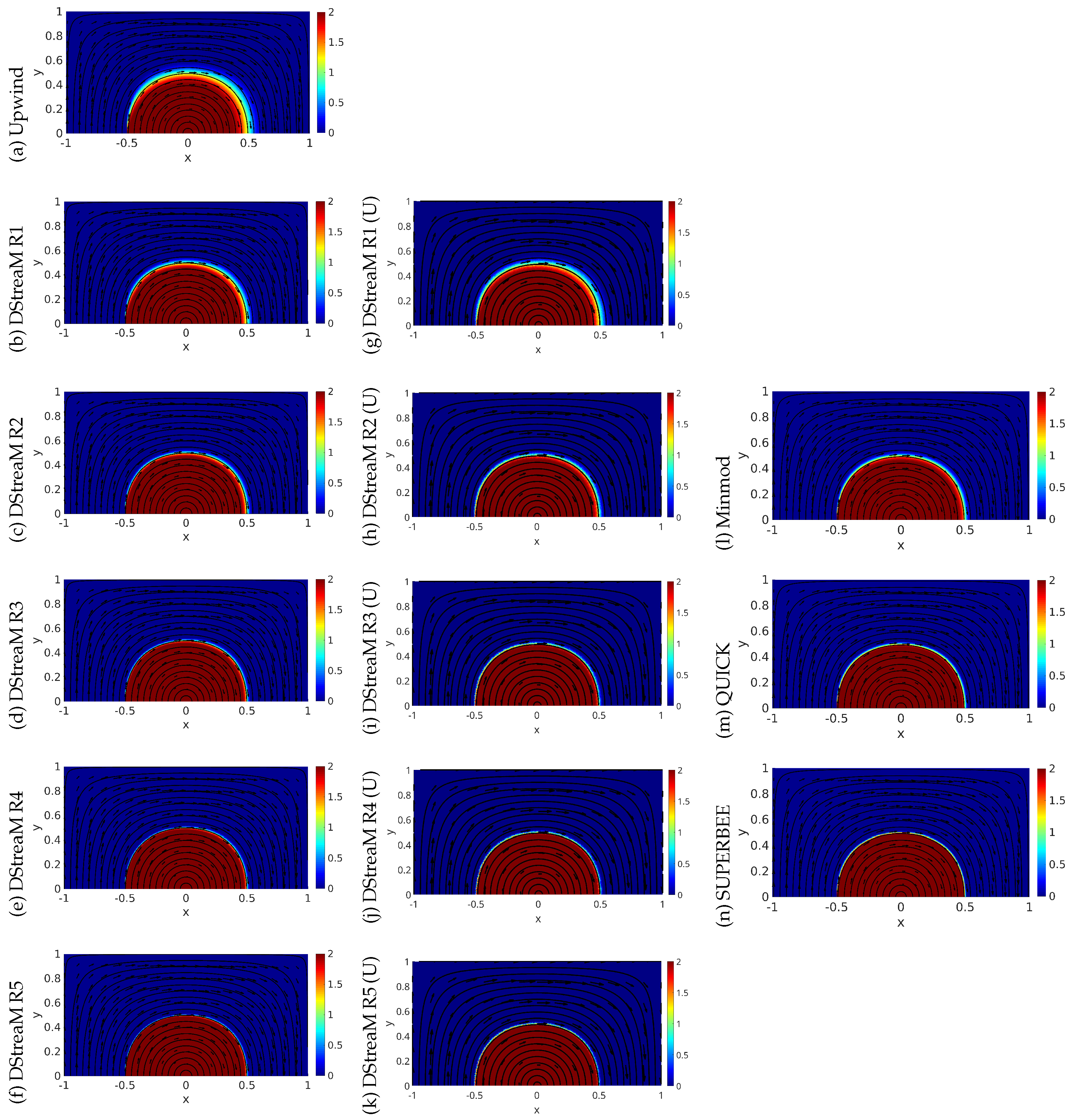
on the coarse mesh. The finer mesh, therefore, represents the curved streamlines by many shorter discrete segments, and DStreaM remains non-oscillatory up to larger radii; see Figure 14. In other words, decreasing allows larger stencil radii R while keeping the discrete streamline aligned with the local flow direction. This property is particularly relevant for applications on unstructured meshes, where smaller spatial steps are typically used in regions of high gradients.
Figure 13.
Smith–Hutton problem: Contours of on a structured Cartesian mesh (a–k,q–s) and an unstructured triangular mesh of comparable resolution (l–p) for and . (a–e) DStreaM with non-limited coefficients, Equation (8), using stencil radii . (f) First-order upwind scheme. (g–k) DStreaM with limited coefficients, Equation (13), with . (l–p) DStreaM (U) on an unstructured triangular mesh with limited coefficients, Equation (13), with . TVD schemes: Minmod (q), QUICK (r), and SUPERBEE (s).
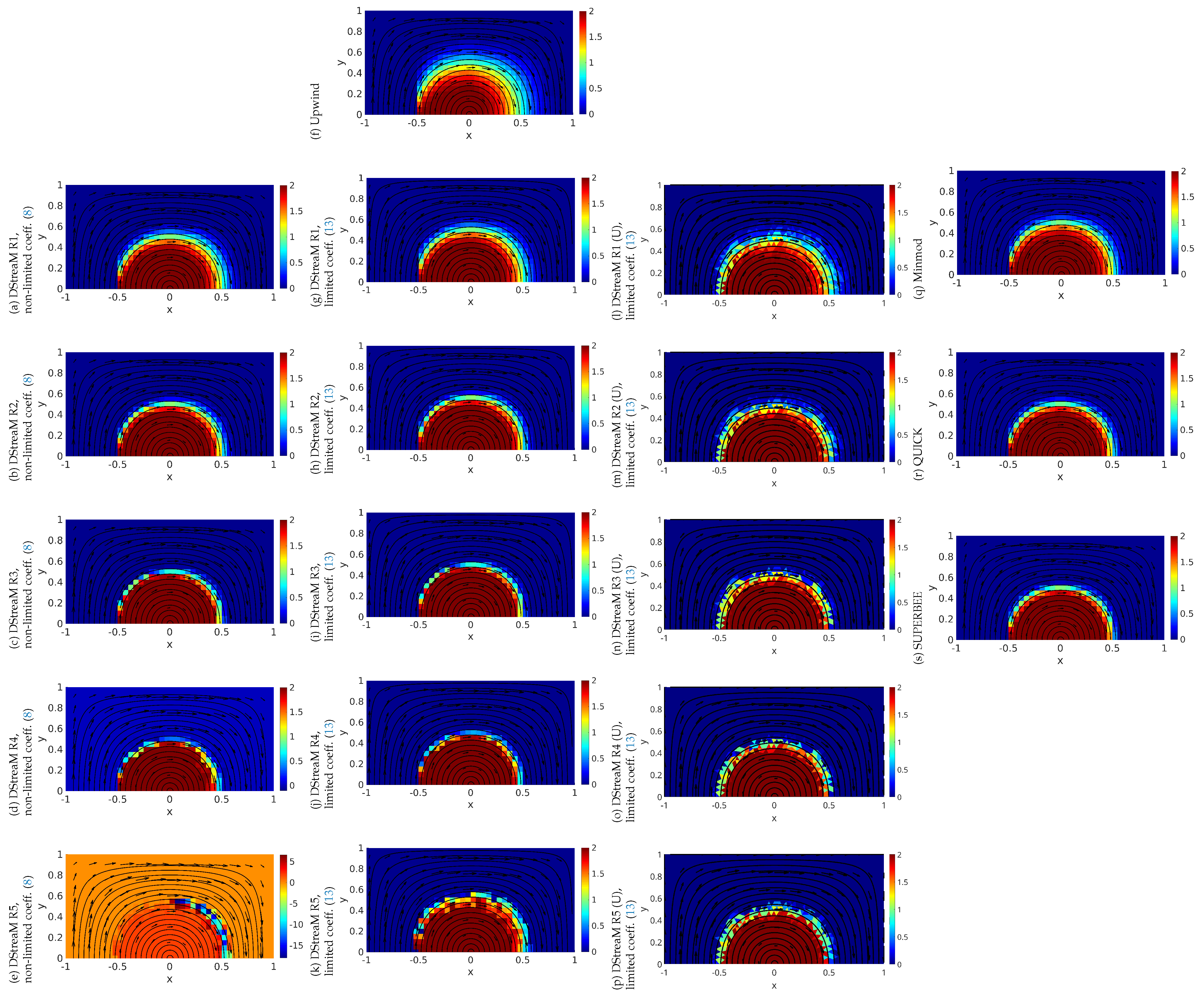
Figure 14.
Smith–Hutton problem: Contours of on a structured Cartesian mesh (a–f,l–n) and an unstructured triangular mesh of comparable resolution (g–k) for and . (a) First-order upwind scheme. (b–f) DStreaM with limited coefficients, Equation (13), with . (g–k) DStreaM (U) on an unstructured triangular mesh with limited coefficients, Equation (13), with . TVD schemes: Minmod (l), QUICK (m), and SUPERBEE (n).
6. Discussion: Mesh Refinement, Efficiency, Conservation, and Applicability
The four convection benchmarks in Section 5 exhibit consistent qualitative trends for DStreaM on both Cartesian and unstructured meshes, with problem-dependent differences in the observed rates and . To avoid repetition, the main common behaviour is discussed first, followed by short case-specific remarks that highlight differences.
6.1. Iterative Convergence and Iteration Counts
For the three uniform-velocity benchmarks (step, double-step, and sinusoidal profiles), the first-order upwind scheme and all structured-mesh DStreaM variants converge in two Gauss–Seidel iterations without under-relaxation (Table 1, Table 2 and Table 3). This behaviour follows from the strictly upstream dependence of the stencil: with a broadly flow-aligned ordering, the discrete operator is close to lower-triangular, and a single iteration acts similarly to a marching update. Cycling the starting corner between successive iterations reduces ordering bias in two dimensions (Section 5). For the TVD schemes, under-relaxation is required, and the iteration counts are one to two orders of magnitude larger: 30–187 iterations depending on the limiter and profile sharpness (Table 1, Table 2 and Table 3).
Keep in mind that iteration count alone is not a sufficient efficiency metric; Table 1, Table 2, Table 3 and Table 4 report wall-clock time for a comparison. The next subsection discusses the per-iteration overhead and its dependence on stencil radius and mesh type.
For the unstructured implementation DStreaM Rk(U), the iteration count is also low for (two iterations in the uniform-velocity benchmarks), while the least-compact case R1(U) requires more iterations (18) on the considered unstructured meshes (Table 1, Table 2 and Table 3). This is consistent with the reduced effectiveness of a single iteration when a strongly flow-aligned ordering is not available on unstructured mesh.
The Smith–Hutton benchmark differs because the velocity direction varies strongly and streamlines are curved (Figure 12a). Consequently, upwind and structured DStreaM converge in four iterations on the mesh, rather than two (Table 4). The TVD schemes again require substantially more iterations (Minmod: 81; QUICK: 62), while SUPERBEE fails to reach the prescribed tolerance within the imposed limit (Table 4).
Figure 12f complements the error and conservation plots by reporting the number of Gauss–Seidel iterations required to satisfy the stopping criterion under mesh refinement. In this curved-streamline benchmark, the upwind scheme and the structured-mesh DStreaM variants reach the prescribed tolerance in a small, essentially mesh-independent number of iterations (four in the reported cases), without under-relaxation, whereas the TVD schemes require substantially more iterations and careful under-relaxation tuning; SUPERBEE converges to the target tolerance only on the coarsest mesh and otherwise stagnates at a much larger maximum change. This behaviour is consistent with Table 4, where the low iteration count for DStreaM is maintained despite its higher per-iteration cost, while the conservative TVD discretisations trade cheaper iterations for markedly longer iteration histories (or stagnation in the SUPERBEE case).
6.2. Compute Time and Unstructured-Mesh Overhead
In all benchmarks, DStreaM reduces iteration count but increases the per-iteration work as the radius grows; this is reflected by the monotone increase in compute time from R1 to R5 on the meshes (Table 1, Table 2 and Table 3). For radii that yield TVD-like sharpness (typically R2–R4 in the uniform-velocity tests), the total time remains competitive with QUICK and SUPERBEE on the same mesh, despite the larger stencil. The unstructured variant DStreaM Rk(U) incurs additional overhead because increasing k requires accessing a larger set of neighbour nodes, and because an unstructured mesh leads to non-contiguous memory access (poor cache locality); for the test cases, this overhead becomes pronounced at a large radius (e.g., R5(U) versus R5 in Table 1, Table 2 and Table 3). A similar trend appears in the Smith–Hutton case on the mesh, where DStreaM Rk(U) is significantly more expensive than structured DStreaM at the same radius (Table 4).
6.3. Mesh Refinement: Error Norms, Observed Rates, and the Role of Smoothness
For all benchmarks, and decrease monotonically under mesh refinement (Figure 9c,d, Figure 10c,d, Figure 11c,d, and Figure 12c,d), and the fitted rates and are listed in Table 1, Table 2, Table 3 and Table 4. The observed order p measures the slope in a relation of the form , while visible profile sharpness at a fixed grid resolution depends strongly on the prefactor C (numerical diffusion level). Consequently, two discretisations can exhibit similar p but very different error magnitudes and solution profiles; this explains why DStreaM may produce TVD-like sharpness even when fitted slopes remain in the sub-unity range for non-smooth benchmarks.
The measured rates depend on (i) profile smoothness and (ii) the complexity/curvature of the characteristics, as follows:
- Step profile: The conservative TVD schemes show the expected ordering in rates (Minmod < QUICK < SUPERBEE; Table 1), while DStreaM on Cartesian meshes exhibits a clear trend of increasing fitted rates with stencil radius (e.g., from at R1 to at R4, and from to ), together with visibly sharper profiles as R increases (Figure 9b). DStreaM R5 reproduces the exact discrete solution and is excluded from the fit. On unstructured meshes, DStreaM Rk(U) shows the same qualitative behaviour (monotone decrease in , and fitted rates improving with R), but with lower observed orders at the same radius (e.g., at R1(U) to at R5(U); Table 1). This reduction is consistent with the geometric variability of the unstructured mesh and a less regular node-update ordering.
- Double-step profile: The TVD schemes again follow the expected ordering in fitted rates (Table 2), and DStreaM produces progressively sharper fronts as R increases (Figure 10b). However, on Cartesian meshes, the fitted DStreaM slopes vary only weakly with radius and remain comparatively modest in this two-front benchmark, indicating that increasing R mainly reduces the error prefactor C (numerical diffusion) rather than producing a substantially steeper asymptotic slope in global norms. DStreaM R5 again reaches round-off-level error and is excluded from the fit. For DStreaM (U), the fitted rates improve more strongly with radius (Table 2), showing that on unstructured meshes, larger radii can increase both the sharpness and the measured convergence slope for this case.
- Sinusoidal profile: For the smooth inlet profile, both DStreaM and TVD schemes achieve higher fitted rates than in the non-smooth tests (Table 3). On Cartesian meshes, DStreaM exhibits a clear improvement with radius and attains near-first-order rates in (up to at R4), while the TVD schemes yield larger fitted rates in this configuration. The unstructured variant DStreaM Rk(U) yields comparable and values for moderate radii, but at a higher wall-clock cost because the neighbourhood traversal is less cache-friendly and requires non-sequential (indirect) memory access.
- Smith–Hutton problem: All methods remain in the sub-first-order regime in this strongly convective, sharply graded case (Table 4), and Figure 13 confirms that accuracy is influenced by the ability to follow curved streamlines. For structured DStreaM, fitted rates decrease for larger radii (Table 4), consistent with the limitation that increasing radius alone does not guarantee higher-order consistency when the discrete streamline segment becomes effectively straighter than the underlying curved characteristic on a given mesh. For DStreaM (U), the fitted values remain around – (Table 4), which can be close to upwind in slope, while still providing visibly sharper fields for appropriate radii (Figure 12, Figure 13 and Figure 14).
Across all benchmarks, is typically smaller than because the norm places more weight on localized peak errors near steep gradients or discontinuities.
6.4. Conservation
The Smith–Hutton case highlights a structural difference between the conservative finite-volume schemes and the present DStreaM formulation. Table 4 (Max change column) and Figure 12e show that the global conservation error (, Equation (32)) remains non-zero for the DStreaM discretisations even when the Gauss–Seidel iteration has converged (Max change ), which is consistent with the non-zero local residuals (Equation (21)) introduced in Section 4.2. On the mesh, typical values are for DStreaM (e.g., for R2 and for R4), with a similar magnitude for DStreaM Rk(U) (Table 4). By contrast, the conservative finite-volume schemes yield much smaller imbalances once converged: on the same mesh, Minmod gives and QUICK gives , while the upwind scheme gives (Table 4) and decreases to round-off level under refinement (order on the mesh, Figure 12e). The larger conservation defect reported for SUPERBEE on the coarse mesh () is consistent with its incomplete convergence at the imposed iteration limit (Max change ), rather than with a loss of conservation in the underlying conservative discretisation.
Reducing the compatibility residuals is a natural next step toward improving conservation within the DStreaM framework.
6.5. Recommended Use and Limitations
Because the present DStreaM discretisation is not conservative by construction, strict global conservation is not guaranteed on general meshes and for non-uniform velocity fields (as quantified by in Figure 12e and Table 4). Therefore, DStreaM is recommended primarily for steady (or pseudo-steady) convection-dominated problems where solution sharpness is the main objective and a small global flux imbalance is acceptable for the quantity of interest, and/or as a predictor (initial guess) for a conservative finite-volume discretisation.
By contrast, DStreaM is not recommended for long-time unsteady simulations in closed or periodic domains (e.g., cavity-type, Couette, or Taylor–Couette configurations) and for applications where strict global conservation is critical (mass/species/energy balances), because a non-zero conservation defect can accumulate in time and lead to drift of integral quantities. For such cases, conservative schemes should be preferred, while DStreaM can still be used as a fast, high-resolution predictor to accelerate the convergence of a conservative solver.
6.6. Sensitivity to Flow Direction, Near-Stagnation Regions, and Rotating Fields
DStreaM selects an upwind triangle based on the local flow direction, and, therefore, inherits the usual sensitivity of streamline/upwind-biased discretisations to uncertainties in the velocity direction. If the prescribed velocity is inaccurate, the selected upstream nodes may not lie on the true characteristic, which primarily affects accuracy (and may increase limiter activity) rather than causing instability in the present steady Gauss–Seidel setting.
When the velocity magnitude becomes very small (), the upwind direction is ill-defined and any purely directional selection becomes ill-conditioned. In practice, this case can be handled by introducing a small tolerance and disabling directional selection when , using instead a purely geometric local choice (e.g., the tightest sector) or retaining the previous iterate. For convection–diffusion problems with , an alternative is to blend to a symmetric (central) discretisation in regions of small local Péclet number.
For rapidly varying or rotating velocity fields, the discrete streamline represents a straight-line surrogate of a curved characteristic over the selected stencil. This limits the usefulness of very large stencil radii: as demonstrated by the Smith–Hutton benchmark, increasing R beyond a moderate value can lead to misalignment with curved streamlines and the appearance of under- and overshoots. Therefore, in strongly curved-streamline regions, smaller radii are preferable.
A dependence on flow direction is inherent to upwind and TVD discretisations; DStreaM shares this general feature because its upstream triangle is selected from the local velocity field.
7. Conclusions
The Discrete Streamline Method (DStreaM) has been presented as a physically motivated discretisation for steady pure-convection problems, built on strictly upstream information transport along a locally defined discrete streamline. The scheme represents the local streamline by an upwind triangle and approximates the convective term via a linear reconstruction whose effective upstream reach is controlled by the stencil radius R. Algorithmic details for upwind-triangle selection on unstructured meshes are also provided, enabling a consistent implementation beyond Cartesian grids.
Across the studied benchmarks, DStreaM delivers high-resolution solutions with low numerical diffusion, comparable in sharpness to classical TVD schemes, while exhibiting very short Gauss–Seidel iteration histories due to its predominantly upstream coupling. Mesh-refinement results based on and error norms confirm monotone error reduction for all cases and show that the observed rates depend primarily on solution smoothness and on the curvature/complexity of the characteristics. In particular, increasing the radius R reduces the error prefactor (diffusion level) and can markedly improve solution quality at a fixed resolution, but it does not, by itself, guarantee a higher formal order of consistency—especially in discontinuous or strongly curved-streamline configurations. Because the larger stencil and directional-selection logic increase per-iteration work, overall efficiency should be judged using wall-clock time in addition to iteration counts; for radii that provide TVD-like sharpness, total compute times remain competitive on Cartesian grids, while unstructured-mesh runs incur a larger overhead due to neighbourhood traversal and reduced memory locality.
A central limitation of the current formulation is conservation. DStreaM is strictly conservative only on a uniform Cartesian mesh with a constant velocity field. For general meshes and/or non-uniform velocities, the coefficient-compatibility residuals do not vanish in general and act as spurious internal sources/sinks in the assembled global balance; consequently, the global boundary–flux imbalance can remain non-zero even after full iterative convergence (as quantified in Section 6.4). Therefore, in its present form, DStreaM is recommended primarily for steady (or pseudo-steady) convection-dominated problems where solution sharpness is the main objective and a small global flux imbalance is acceptable, and/or as a fast, high-quality predictor (initial guess) for a conservative finite-volume discretization. It is not recommended as a stand-alone scheme for long-time unsteady simulations or for applications where strict global conservation is critical.
Future developments should focus on (i) enforcing coefficient compatibility to reduce and achieve strict conservation on general meshes and non-uniform velocity fields; (ii) improving robustness for rapidly varying directions and near-degenerate local velocity states; (iii) extending the approach to transient and coupled transport systems within fully conservative CFD solvers; and (iv) improving cost-effectiveness on unstructured meshes (data structures, traversal strategies, and parallel implementations), alongside exploring higher-order streamline-aligned reconstructions that better follow curved characteristics.
Supplementary Materials
The following supporting information is provided as Supplementary Materials (ZIP archive). The canonical external record is hosted on Figshare (DOI: https://doi.org/10.6084/m9.figshare.31119316, accessed on 19 January 2026). A mirror copy is also available on Zenodo (https://zenodo.org/records/18331392, accessed on 19 January 2026). The MD5 checksum of the ZIP archive is 4da4b269ed3471aa3b08880fbcfb3dab). The archive contains the root directory paper_suplementary_materials/ with: (i) C++ source codes (with Makefiles and input files) for DStreaM on structured Cartesian meshes and on unstructured meshes, compiled and tested on Linux (Debian 12), together with MATLAB 2020b scripts for reading/plotting results; (ii) a reference TVD implementation for the 2D convection problem; (iii) reproducibility folders for each benchmark case (including InputData.txt, representative output fields, log files with iterations/timings, and MATLAB/Python/Bash post-processing scripts); (iv) mesh-convergence datasets for the Smith–Hutton case (L1/L2 log–log plot data); and (v) Wolfram Mathematica 14.0 derivations (notebook .nb and companion PDF. Top-level contents of paper_suplementary_materials/: DStreaM_code; DStreaM_code_unstuctured_mesh; 2D_convection_problem_TVD_code; Convection_of_a_step_profile_problem_DStreaM; Convection_of_a_step_profile_problem_DStreaM_unstructured; Convection_of_a_step_profile_problem_TVD; Convection_of_a_step_profile_problem_DStreaM_mesh_convergence_L1_L2_log-log_plot_data; Convection_of_a_step_profile_problem_DStreaM_unstructured_mesh_convergence_L1_L2_log-log_plot_data; Convection_of_a_step_profile_problem_TVD_mesh_convergence_L1_L2_log-log_plot_data; Convection_of_a_double_step_profile_problem_DStreaM; Convection_of_a_double_step_profile_problem_DStreaM_unstructured; Convection_of_a_double_step_profile_problem_TVD; Convection_of_a_double_step_profile_problem_DStreaM_mesh_convergence_L1_L2_log-log_plot_data; Convection_of_a_double_step_profile_problem_DStreaM_unstructured_mesh_convergence_L1_L2_log-log_plot_data; Convection_of_a_double_step_profile_problem_TVD_mesh_convergence_L1_L2_log-log_plot_data; Convection_of_a_sinusoidal_profile_problem_DStreaM; Convection_of_a_sinusoidal_profile_problem_DStreaM_unstructured; Convection_of_a_sinusoidal_profile_problem_TVD; Convection_of_a_sinusoidal_profile_problem_DStreaM_mesh_convergence_L1_L2_log-log_plot_data; Convection_of_a_sinusoidal_profile_problem_DStreaM_unstructured_mesh_convergence_L1_L2_log-log_plot_data; Convection_of_a_sinusoidal_profile_problem_TVD_mesh_convergence_L1_L2_log-log_plot_data; Smith_Hutton_profile_problem_DStreaM; Smith_Hutton_profile_problem_DStreaM_unstructured; Smith_Hutton_profile_problem_TVD; Smith_Hutton_profile_problem_DStreaM_mesh_convergence_L1_L2_log-log_plot_data; Smith_Hutton_profile_problem_DStreaM_unstructured_mesh_convergence_L1_L2_log-log_plot_data; Smith_Hutton_profile_problem_TVD_mesh_convergence_L1_L2_log-log_plot_data; Simple_Conv_equation_derive_General_with_Barycentric_coordinates_and_constant_velocities_ua_va.nb; Simple_Conv_equation_derive_General_with_Barycentric_coordinates_and_constant_velocities_ua_va.pdf.
Funding
This work was accomplished with financial support from the Bulgarian research fund, grant KP-06-N72/7, 2023. The work was partially supported by the Centre of Excellence in Informatics and ICT under the Grant No BG16RFPR002-1.014-0018-C01, financed by the Research, Innovation and Digitalization for Smart Transformation Programme 2021–2027 and co-financed by the European Union.
Institutional Review Board Statement
Not applicable.
Informed Consent Statement
Not applicable.
Data Availability Statement
The original contributions presented in this study are included in the Supplementary Material. Further inquiries can be directed to the corresponding author.
Conflicts of Interest
The author declares no conflicts of interest.
Appendix A. Derivation of the DStreaM Nodal Relation Using Barycentric Coordinates
In this appendix, the discrete relation (7) for the nodal value is derived by integrating the pure-convection equation over an upwind triangular region and using barycentric (area) coordinates. The derivation makes explicit the connection between the continuous equation and the DStreaM approximation.
The complete symbolic derivation is also provided in the Supplementary Materials as a Wolfram Mathematica .nb notebook and its PDF export:
- Simple_Conv_equation_derive_General_with_Barycentric_coordinates_and_constant_velocities_ua_va.nb
- Simple_Conv_equation_derive_General_with_Barycentric_coordinates_and_constant_velocities_ua_va.pdf
Appendix A.1. Upwind Triangular Region and Barycentric Coordinates
Consider an upwind triangular region T with vertices
associated with nodal values
Let denote the area of the upwind triangle. In the DStreaM approximation, the scalar field is represented locally by a linear shape function
chosen such that
An equivalent representation uses barycentric (area) coordinates defined by
and the affine mapping
In these coordinates, the linear interpolant can be written as
For later use, the standard expressions for the gradients of the barycentric shape functions are recalled, as follows:
where the area V is
Appendix A.2. Gradient of the Shape Function
Appendix A.3. Mapping to a Reference Triangle and Explicit Integrals
To make the integration explicit, the upwind triangular region T is mapped to the reference triangle
via the affine mapping
The Jacobian matrix of this mapping is
with determinant
Hence, the area element transforms as
and for any scalar function , the following relation holds:
In the present derivation, the derivatives and are constant on T, so the integrals reduce to
If one wishes to show the explicit limits as in a symbolic computation, this can be written as
and analogously for .
Appendix A.4. Integral Form of the Convection Equation on the Upwind Triangle
In the DStreaM approximation, the velocity is taken to be constant over the upwind triangular region,
and the scalar is approximated by . The steady pure-convection equation in conservative form is
Substituting , , and and integrating over the upwind triangular region T yields
Using (A14) and dividing by V yields the local condition
Substituting the expressions from (A9) gives a linear relation between the three nodal values,
with
Solving (A19) for gives
Introducing
The DStreaM nodal relation is recovered
with coefficients and consistent with Equations (7) and (8) in the main text.
References
- Boris, J.P.; Book, D.L. Flux-corrected transport. I. SHASTA, a fluid transport algorithm that works. J. Comput. Phys. 1973, 11, 38–69. [Google Scholar] [CrossRef] [Scilit]
- Boris, J.P.; Book, D.L. Solution of continuity equations by the method of flux-corrected transport. In Controlled Fusion; Killeen, J., Ed.; Academic Press: New York, NY, USA, 1976; pp. 85–129. [Google Scholar]
- van Leer, B. Towards the ultimate conservative difference scheme. II. Monotonicity and conservation combined in a second-order scheme. J. Comput. Phys. 1974, 14, 361–370. [Google Scholar] [CrossRef] [Scilit]
- Leer, B.V. Towards the ultimate conservative difference scheme III. Upstream-centered finite-difference schemes for ideal compressible flow. J. Comput. Phys. 1977, 23, 263–275. [Google Scholar] [CrossRef] [Scilit]
- Leer, B.V. Towards the ultimate conservative difference scheme. IV. A new approach to numerical convection. J. Comput. Phys. 1977, 23, 276–299. [Google Scholar] [CrossRef] [Scilit]
- van Leer, B. Towards the ultimate conservative difference scheme. V. A second-order sequel to Godunov’s method. J. Comput. Phys. 1979, 32, 101–136. [Google Scholar] [CrossRef] [Scilit]
- Harten, A. High resolution schemes for hyperbolic conservation laws. J. Comput. Phys. 1983, 49, 357–393. [Google Scholar] [CrossRef] [Scilit]
- Harten, A. On a Class of High Resolution Total-Variation-Stable Finite-Difference Schemes. SIAM J. Numer. Anal. 1984, 21, 1–23. [Google Scholar] [CrossRef] [Scilit]
- Sweby, P.K. High Resolution Schemes Using Flux Limiters for Hyperbolic Conservation Laws. SIAM J. Numer. Anal. 1984, 21, 995–1011. [Google Scholar] [CrossRef] [Scilit]
- Roe, P.L. Some contributions to the modelling of discontinuous flows. Lect. Appl. Math. 1985, 22, 163–193. [Google Scholar]
- Osher, S.; Chakravarthy, S. High Resolution Schemes and the Entropy Condition. SIAM J. Numer. Anal. 1984, 21, 955–984. [Google Scholar] [CrossRef] [Scilit]
- Zijlema, M. ON THE CONSTRUCTION OF A THIRD-ORDER ACCURATE MONOTONE CONVECTION SCHEME WITH APPLICATION TO TURBULENT FLOWS IN GENERAL DOMAINS. Int. J. Numer. Methods Fluids 1996, 22, 619–641. [Google Scholar] [CrossRef] [Scilit]
- Arora, M.; Roe, P.L. A Well-Behaved TVD Limiter for High-Resolution Calculations of Unsteady Flow. J. Comput. Phys. 1997, 132, 3–11. [Google Scholar] [CrossRef] [Scilit]
- Čada, M.; Torrilhon, M. Compact third-order limiter functions for finite volume methods. J. Comput. Phys. 2009, 228, 4118–4145. [Google Scholar] [CrossRef] [Scilit]
- Ferreira, V.; de Queiroz, R.; Lima, G.; Cuenca, R.; Oishi, C.; Azevedo, J.; McKee, S. A bounded upwinding scheme for computing convection-dominated transport problems. Comput. Fluids 2012, 57, 208–224. [Google Scholar] [CrossRef] [Scilit]
- Zhang, D.; Jiang, C.; Liang, D.; Cheng, L. A review on TVD schemes and a refined flux-limiter for steady-state calculations. J. Comput. Phys. 2015, 302, 114–154. [Google Scholar] [CrossRef] [Scilit]
- Kriel, A. Error analysis of flux limiter schemes at extrema. J. Comput. Phys. 2017, 328, 371–386. [Google Scholar] [CrossRef] [Scilit]
- Sukhinov, A.; Chistyakov, A.; Kuznetsova, I.; Belova, Y.; Rahimbaeva, E. Development and Research of a Modified Upwind Leapfrog Scheme for Solving Transport Problems. Mathematics 2022, 10, 3564. [Google Scholar] [CrossRef] [Scilit]
- Sukhinov, A.; Chistyakov, A.; Kuznetsova, I.; Belova, Y.; Rahimbaeva, E. Solving Hydrodynamic Problems Based on a Modified Upwind Leapfrog Scheme in Areas with Complex Geometry. Mathematics 2022, 10, 3248. [Google Scholar] [CrossRef] [Scilit]
- Dostál, J.; Havlena, V. Mixed Mesh Finite Volume Method for 1D Hyperbolic Systems with Application to Plug-Flow Heat Exchangers. Mathematics 2021, 9, 2609. [Google Scholar] [CrossRef] [Scilit]
- Quinga, S.; Pavon, W.; Ortiz, N.; Calvopiña, H.; Yépez, G.; Quinga, M. Numerical Solution of the Nonlinear Convection–Diffusion Equation Using the Fifth Order Iterative Method by Newton–Jarratt. Mathematics 2025, 13, 1164. [Google Scholar] [CrossRef] [Scilit]
- Majima, Y.; Wakimura, H.; Aoki, T.; Xiao, F. A new high-fidelity Total Variation Diminishing scheme based on the Boundary Variation Diminishing principle for compressible flows. Comput. Fluids 2023, 266, 106070. [Google Scholar] [CrossRef] [Scilit]
- Deng, X. A new open-source library based on novel high-resolution structure-preserving convection schemes. J. Comput. Sci. 2023, 74, 102150. [Google Scholar] [CrossRef] [Scilit]
- Raithby, G. Skew upstream differencing schemes for problems involving fluid flow. Comput. Methods Appl. Mech. Eng. 1976, 9, 153–164. [Google Scholar] [CrossRef] [Scilit]
- Raithby, G. A critical evaluation of upstream differencing applied to problems involving fluid flow. Comput. Methods Appl. Mech. Eng. 1976, 9, 75–103. [Google Scholar] [CrossRef] [Scilit]
- Hassan, Y.A.; Rice, J.G.; Kim, J.H. A STABLE MASS-FLOW-WEIGHTED TWO-DIMENSIONAL SKEW UPWIND SCHEME. Numer. Heat Transf. 1983, 6, 395–408. [Google Scholar] [CrossRef] [Scilit]
- Schneider, G.E.; Raw, M.J. A SKEWED, POSITIVE INFLUENCE COEFFICIENT UPWINDING PROCEDURE FOR CONTROL-VOLUME-BASED FINITE-ELEMENT CONVECTION-DIFFUSION COMPUTATION. Numer. Heat Transf. 1986, 9, 1–26. [Google Scholar] [CrossRef] [Scilit]
- Patel, M.K.; Cross, M.; Markatos, N.C. An assessment of flow oriented schemes for reducing ‘false diffusion’. Int. J. Numer. Methods Eng. 1988, 26, 2279–2304. [Google Scholar] [CrossRef] [Scilit]
- Busnaina, A.; Zheng, X.; Sharif, M. A modified skew upwind scheme for fluid flow and heat transfer computations. Appl. Math. Model. 1991, 15, 425–432. [Google Scholar] [CrossRef] [Scilit]
- Carey, C.; Scanlon, T.J.; Fraser, S.M. The Reduction of False Diffusion in the Simulation of Vortex Shedding. Proc. Inst. Mech. Eng. Part C J. Mech. Eng. Sci. 1992, 206, 399–406. [Google Scholar] [CrossRef] [Scilit]
- Carey, C.; Scanlon, T.; Fraser, S. SUCCA-an alternative scheme to reduce the effects of multidimensional false diffusion. Appl. Math. Model. 1993, 17, 263–270. [Google Scholar] [CrossRef] [Scilit]
- Darwish, M.; Moukalled, F. A new approach for building bounded skew-upwind schemes. Comput. Methods Appl. Mech. Eng. 1996, 129, 221–233. [Google Scholar] [CrossRef] [Scilit]
- Leonard, B.P. Simple high-accuracy resolution program for convective modelling of discontinuities. Int. J. Numer. Methods Fluids 1988, 8, 1291–1318. [Google Scholar] [CrossRef] [Scilit]
- Ogedengbe, E.O.B.; Naterer, G.F. Non-Inverted Skew Upwind Scheme for Three-Dimensional Convective Transport. Numer. Heat Transf. Part B Fundam. 2004, 46, 141–164. [Google Scholar] [CrossRef] [Scilit]
- Ogedengbe, E.O.B. Non-Inverted Skew Upwind Scheme for Numerical Heat Transfer and Fluid Flow Simulations. Ph.D. Thesis, University of Manitoba, Winnipeg, MB, Canada, 2006. [Google Scholar]
- Karadimou, D.; Markatos, N. A novel flow-oriented discretization scheme for reducing false diffusion in three-dimensional (3D) flows: An application in the indoor environment. Atmos. Environ. 2012, 61, 327–339. [Google Scholar] [CrossRef] [Scilit]
- Chung, T.J. Computational Fluid Dynamics; Cambridge University Press: Cambridge, UK, 2002. [Google Scholar] [CrossRef] [Scilit]
- Loitsiansky, L.G. Fluid and Gas Mechanics, 7th ed.; Drofa: Moscow, Russia, 2003; p. 840. [Google Scholar]
- White, F.M. Viscous Fluid Flow, 3rd ed.; Mcgraw Hill Series in Mechanical Engineering; McGraw-Hill Education: Columbus, OH, USA, 2005; p. 656. [Google Scholar]
- Geuzaine, C.; Remacle, J.F. Gmsh: A 3-D finite element mesh generator with built-in pre- and post-processing facilities. Int. J. Numer. Methods Eng. 2009, 79, 1309–1331. [Google Scholar] [CrossRef] [Scilit]
- Smith, R.M.; Hutton, A.G. THE NUMERICAL TREATMENT OF ADVECTION: A PERFORMANCE COMPARISON OF CURRENT METHODS. Numer. Heat Transf. 1982, 5, 439–461. [Google Scholar] [CrossRef] [Scilit]
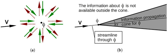
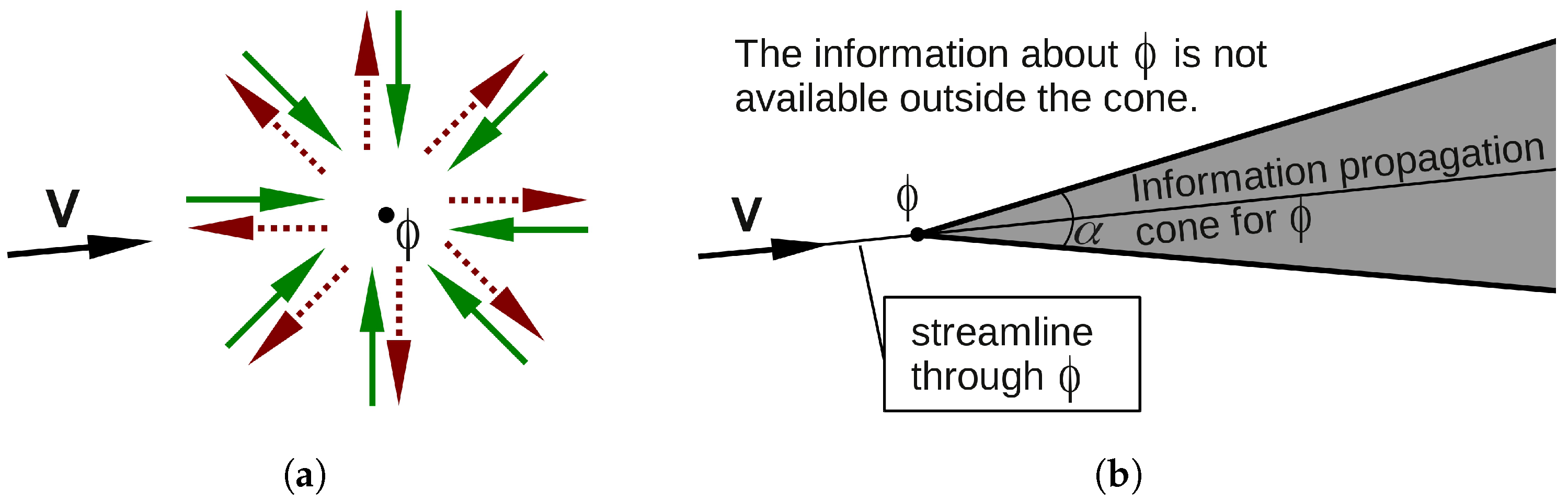
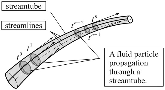
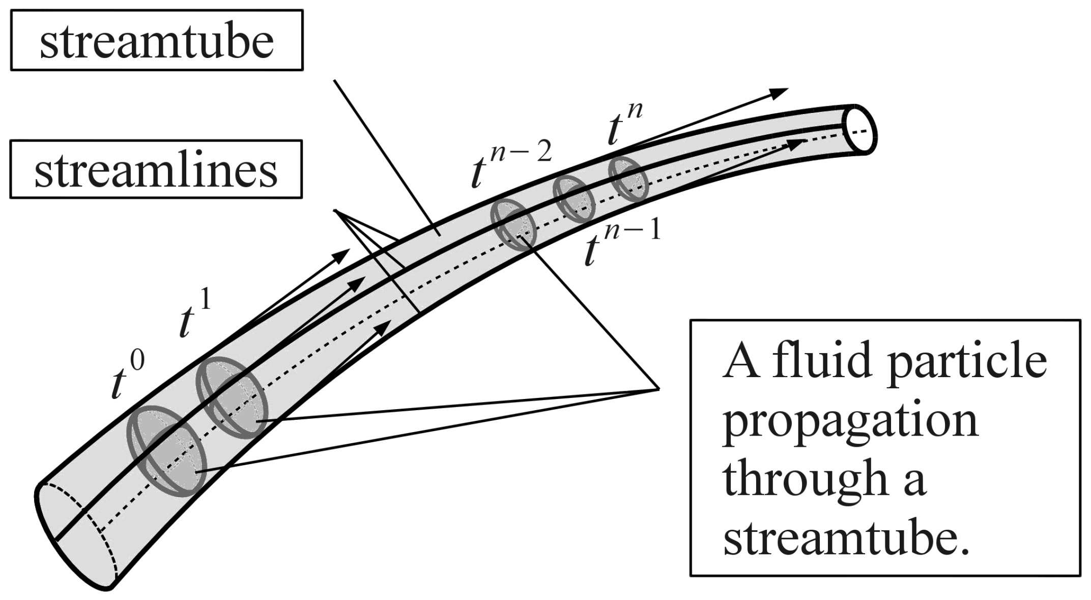
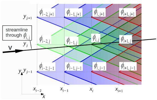
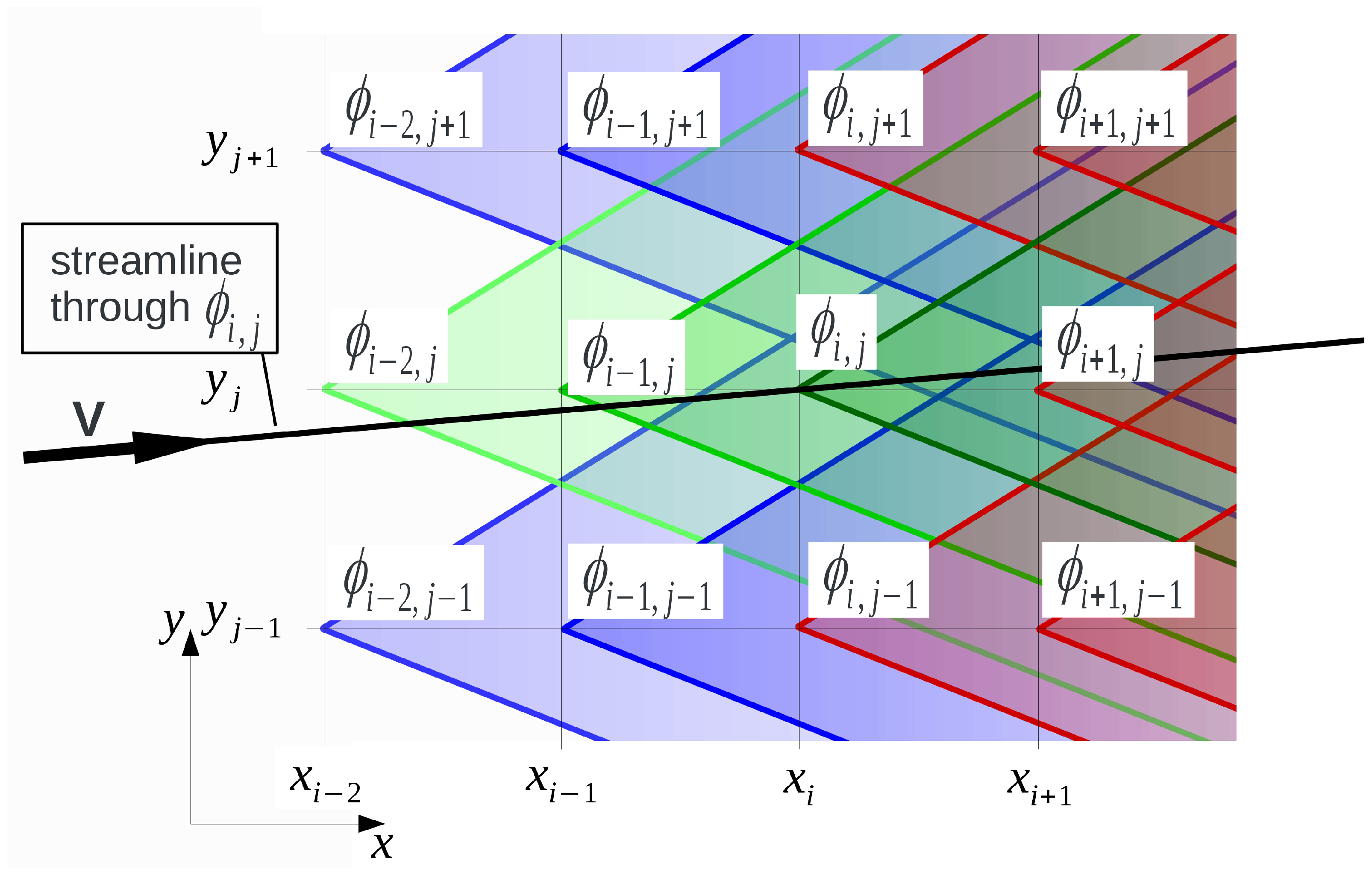
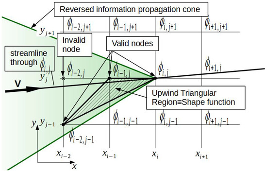
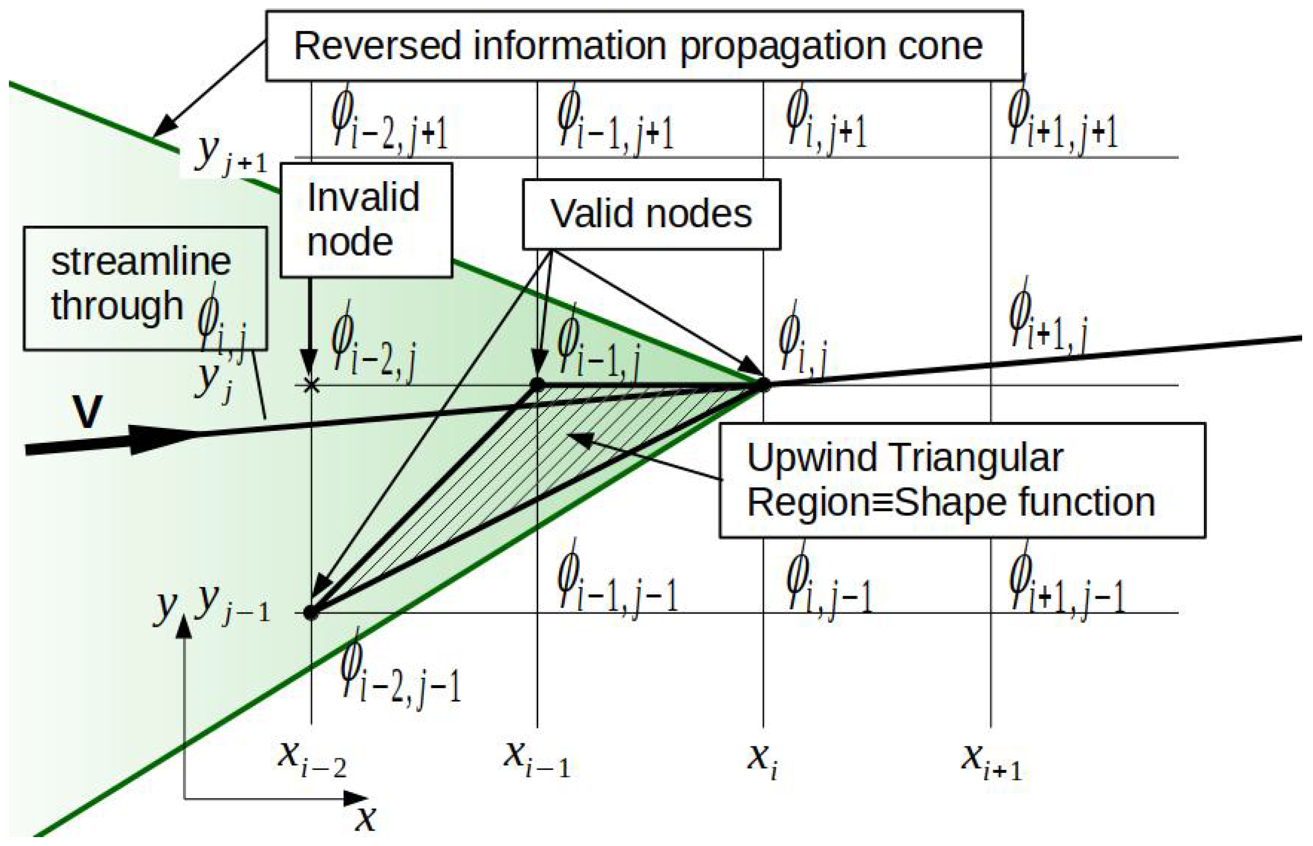


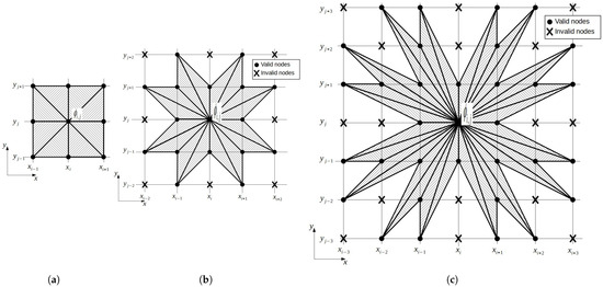
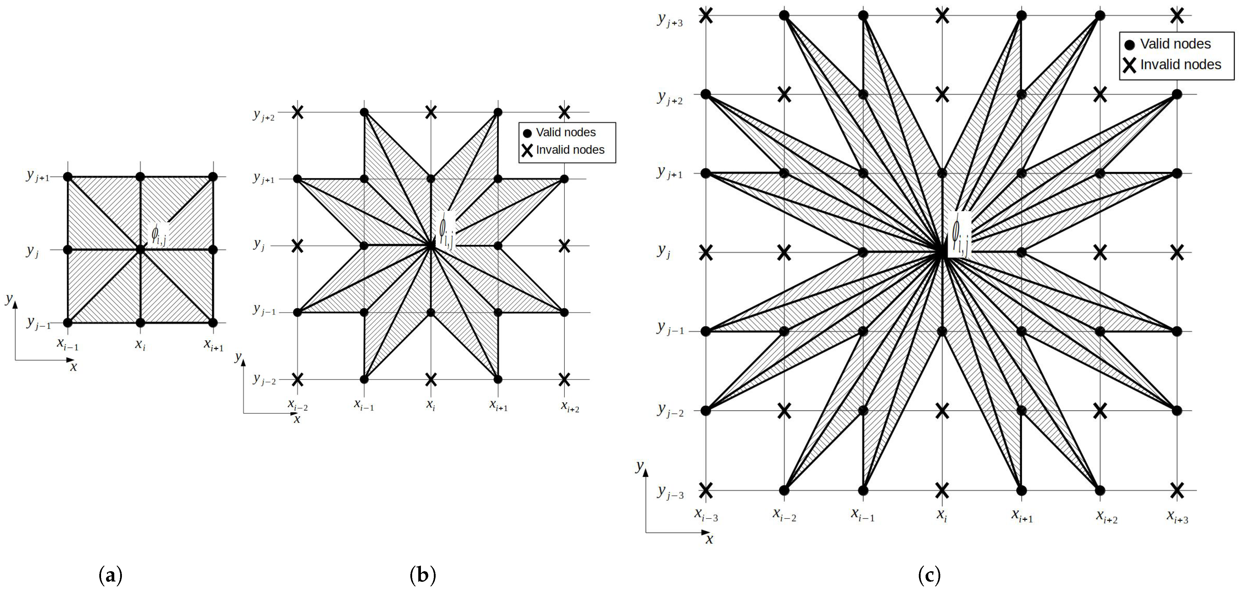
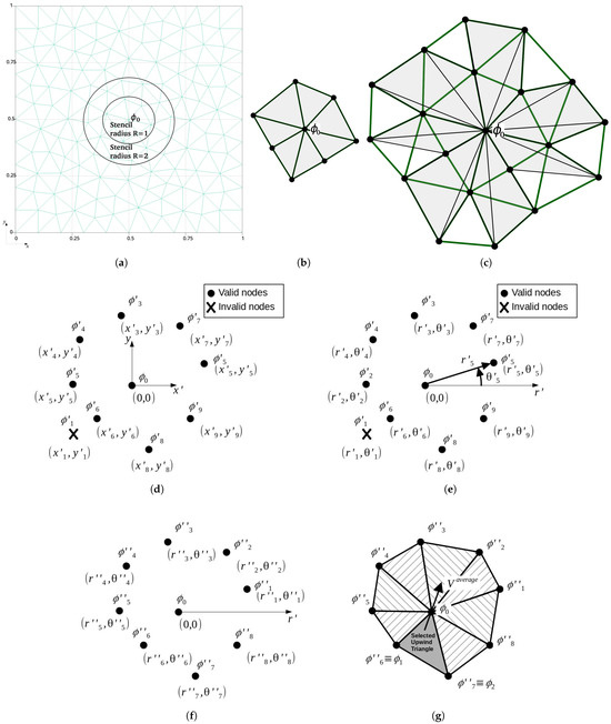
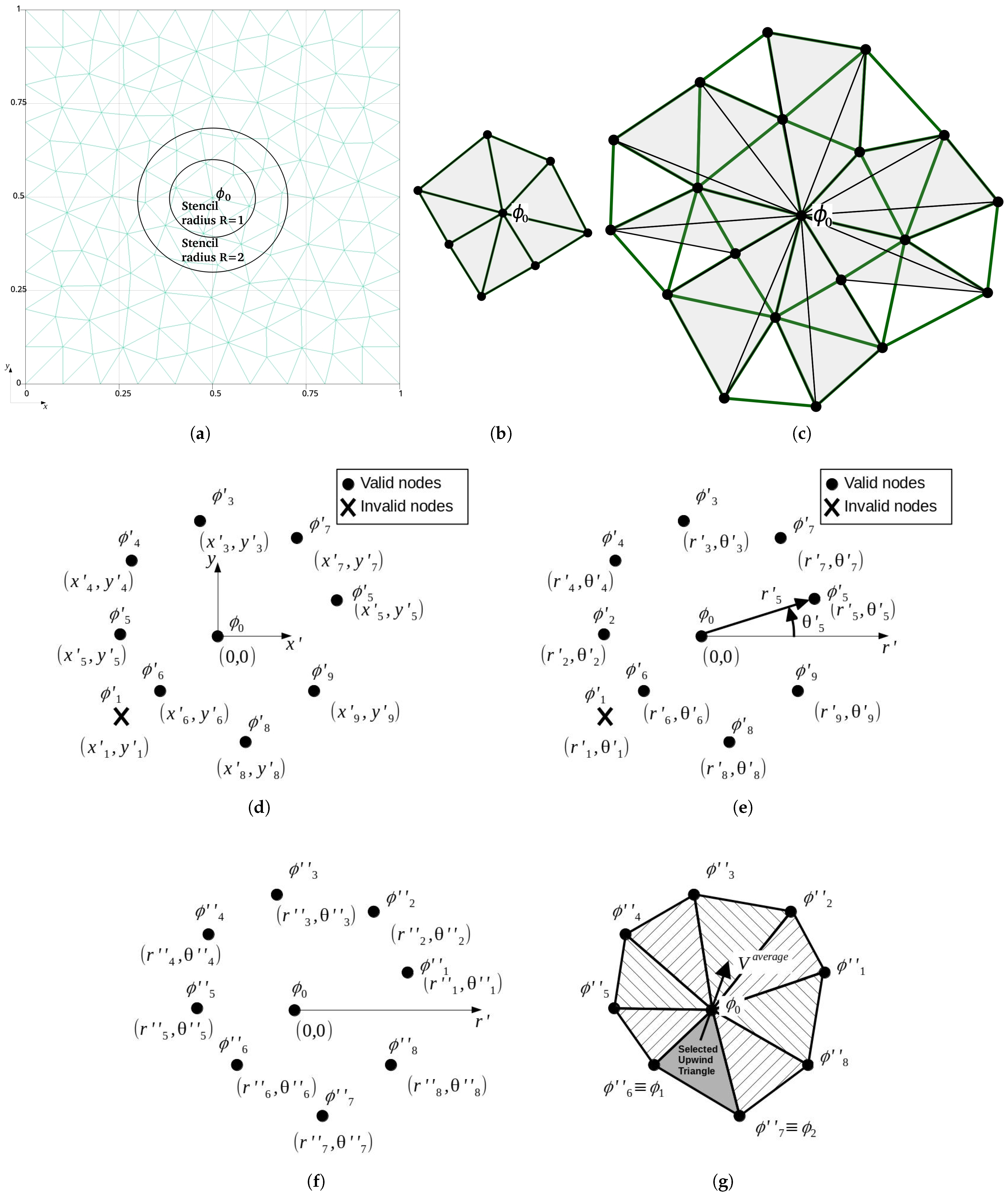
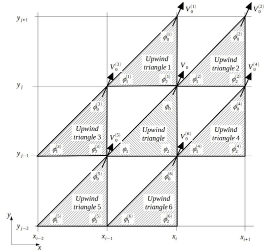
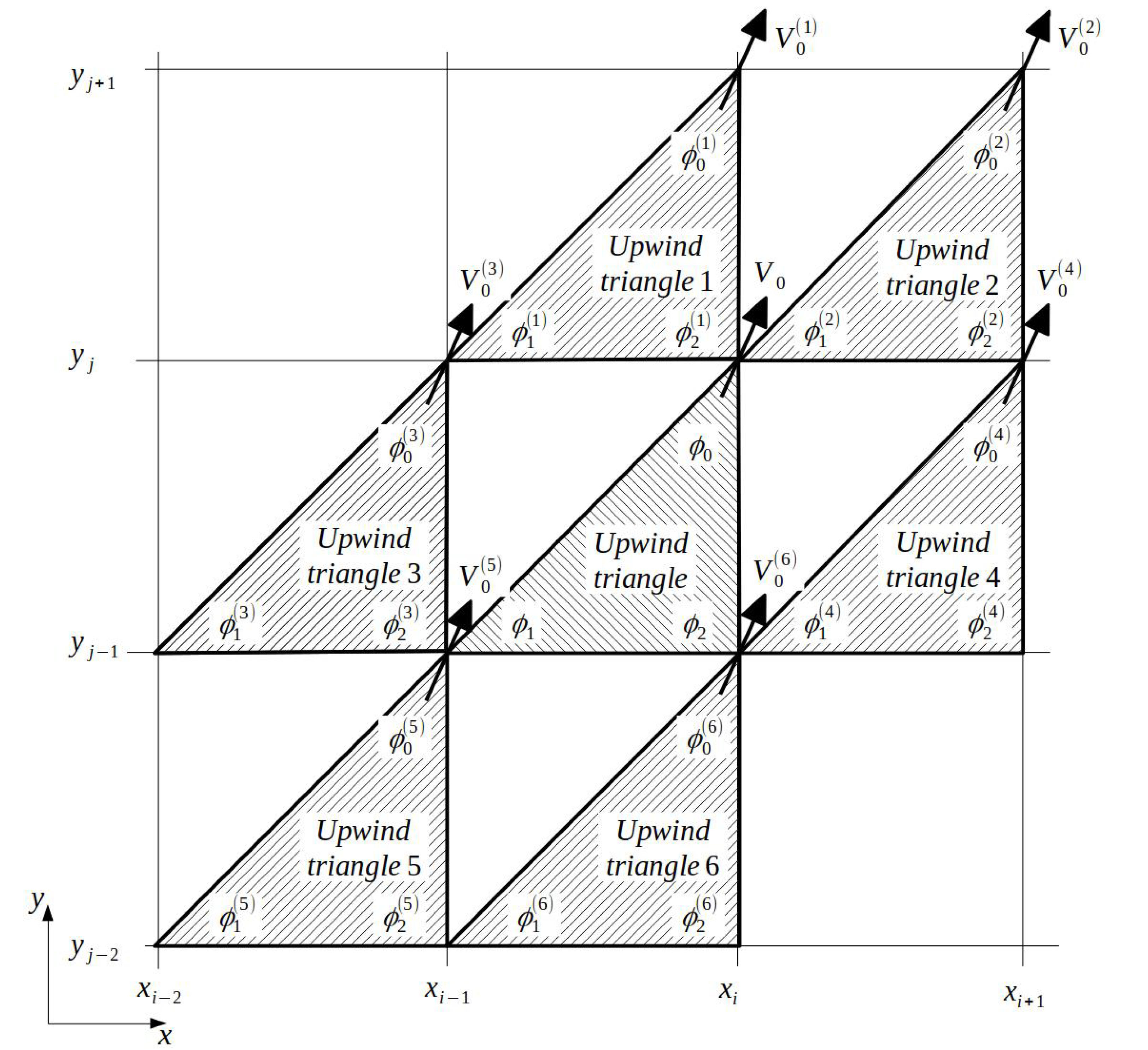
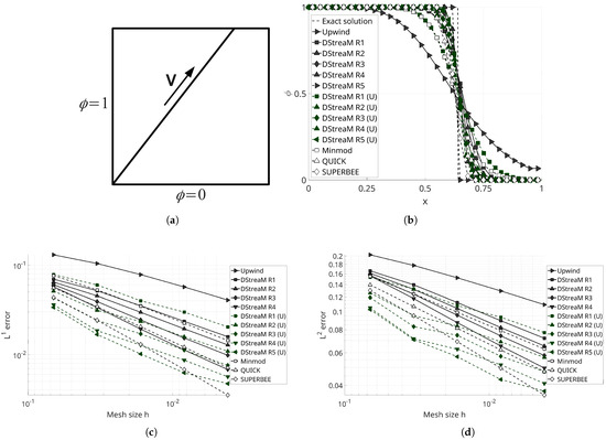
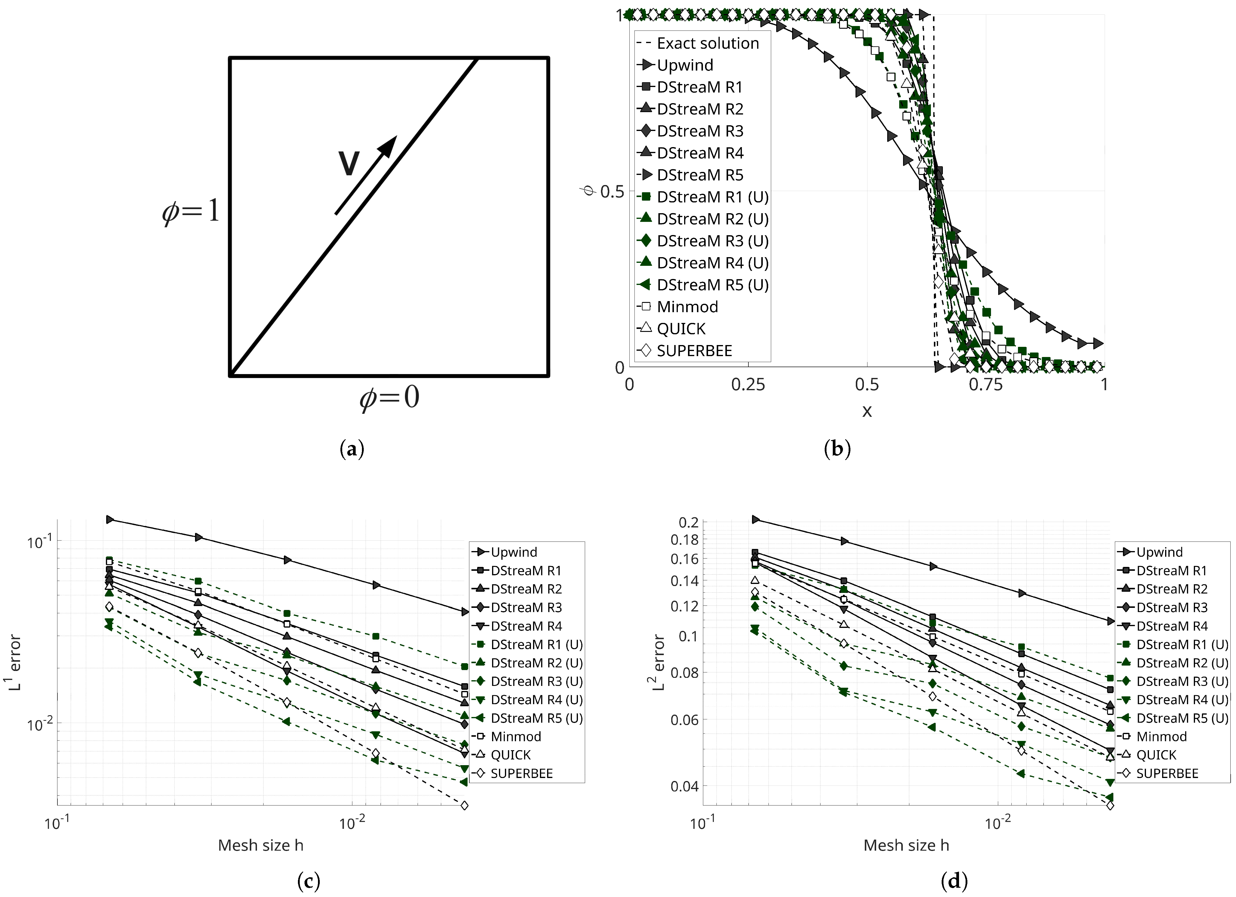
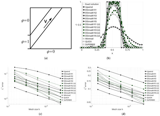
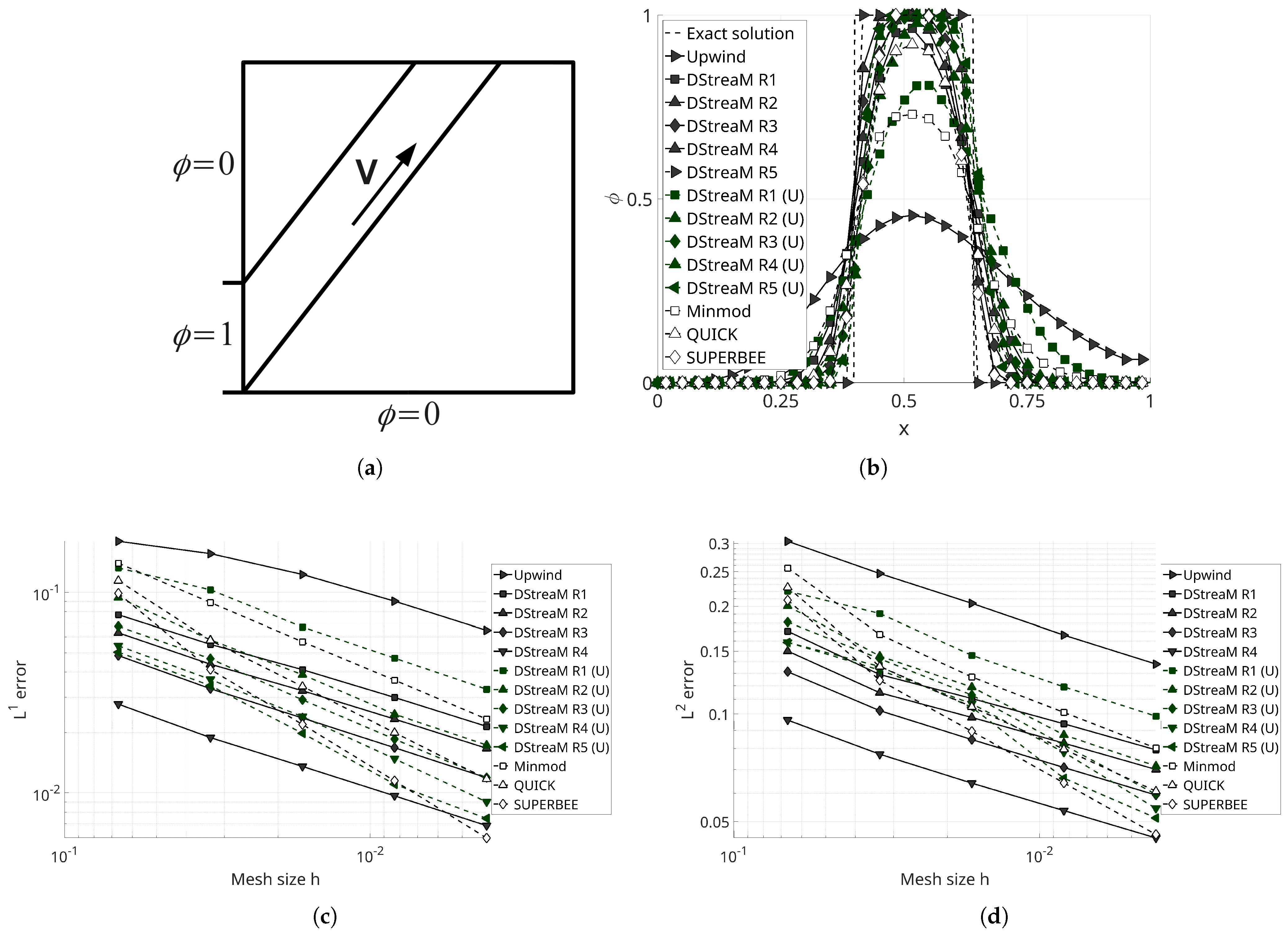
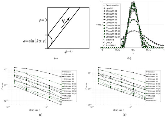
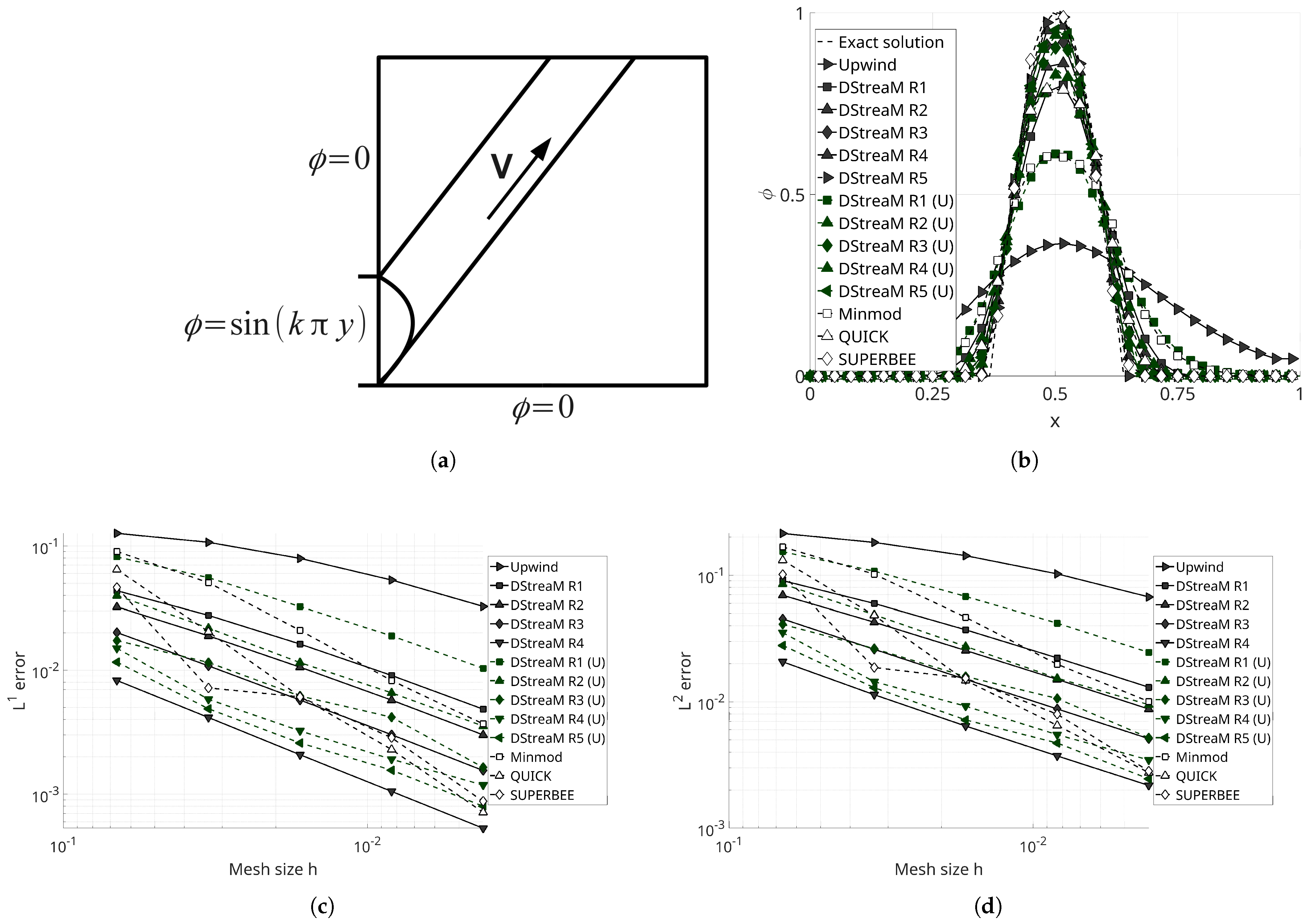
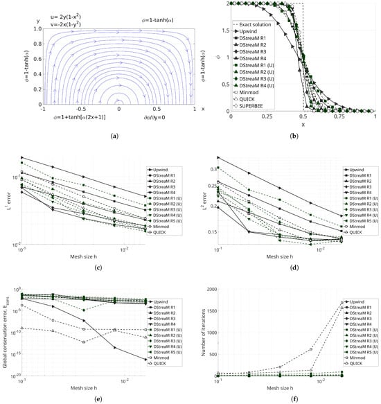
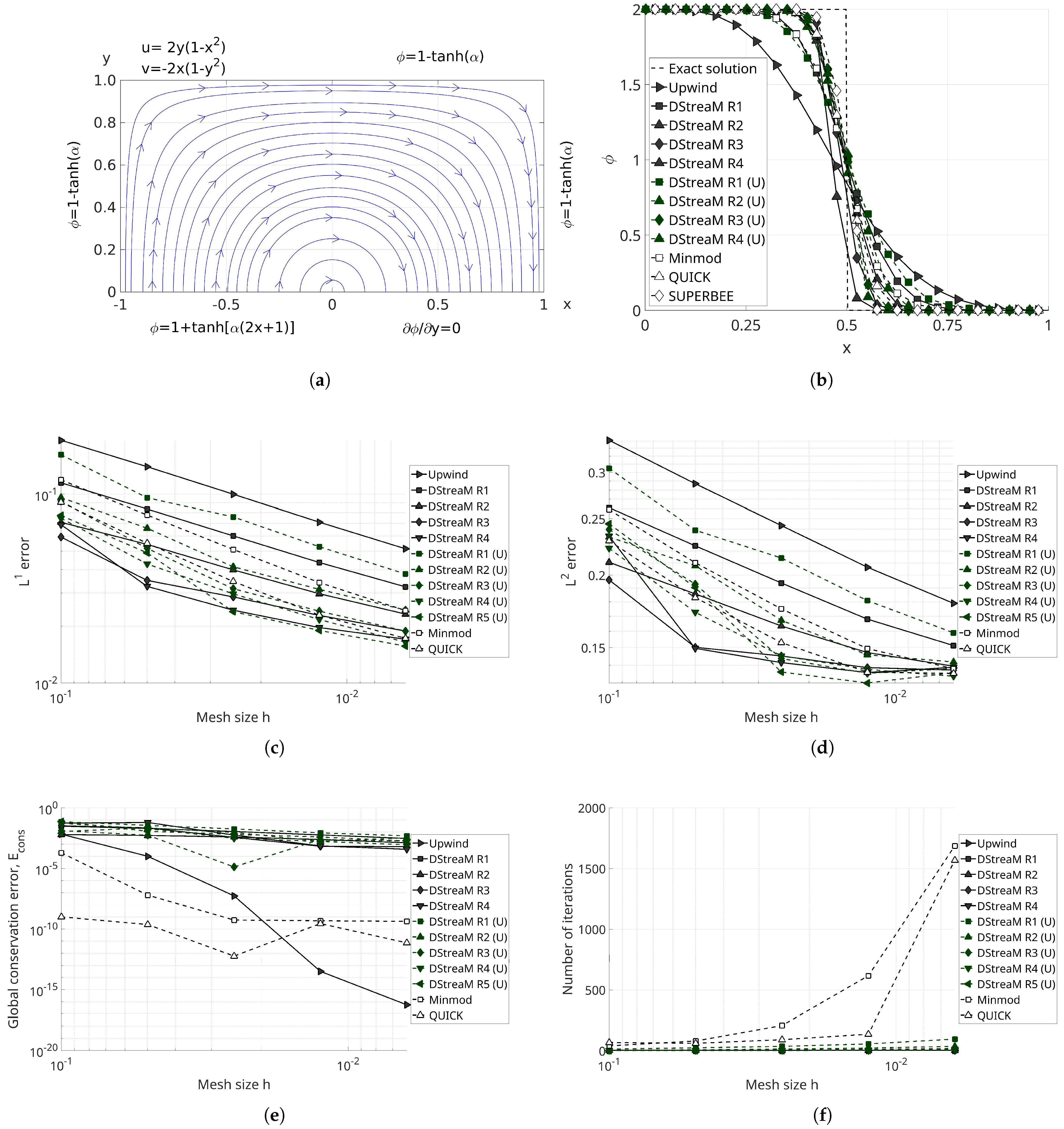

Disclaimer/Publisher’s Note: The statements, opinions and data contained in all publications are solely those of the individual author(s) and contributor(s) and not of MDPI and/or the editor(s). MDPI and/or the editor(s) disclaim responsibility for any injury to people or property resulting from any ideas, methods, instructions or products referred to in the content. |
© 2026 by the author. Licensee MDPI, Basel, Switzerland. This article is an open access article distributed under the terms and conditions of the Creative Commons Attribution (CC BY) license.