


Abstract
In this paper, recurrent MAP flows are constructed using a Markov modulated Poisson process. Given the deterministic dead time for these flows, recurrent observation flows are determined. Dead times are estimated as the minimum distances between adjacent observation times. The validity of these estimates is proved using an upper bound for the jump size of the random walk defined by the recurrent MAP flow. This upper bound is investigated using the continuity theorem for uniformly convergent series of continuous functions and the Weierstrass theorem on the maximum of a continuous function on a segment and has a form of geometric progression. Denominator of this geometric progression is also estimated.
MSC:
05C81; 60J28
1. Introduction
The problem of estimating dead time when monitoring flows in queueing systems is of great practical and theoretical interest. A large number of publications in the international scientific literature have been devoted to this problem: from early [1,2,3] to modern [4,5,6,7]. First and foremost, we should note the important applied work of A.M. Gortsev with colleagues [8,9,10,11,12]. These papers examine a generalized semisynchronous flow operating under conditions where the dead-time duration is an unknown fixed value. A comparison is made between the quality of estimates obtained using the maximum likelihood method (ML) and the method of moments (MM). The solution to the optimization problem is proven to be the ML estimate of the minimum intervals between adjacent observation points. It should be noted that dead time is determined solely by the operation of the device itself, and not by the operation of the queueing system receiving the flow of customers.
The most recent work of A.M. Gortsev and his collaborators on estimating the dead time of observations of Poisson flows with varying intensity is presented in articles [9,10,11,12,13]. In these articles the distribution densities of intervals between adjacent requests of these recurrent flows are explicitly calculated. The technique for obtaining such results could not be extended to the case where the number of states of the Poisson flow determining its intensity is greater than two. However, in [14] the recurrence conditions for the MAP flow (without taking dead time into account) were obtained, which motivated our research. For the reader’s convenience, the MAP flow model is successively complicated, progressing from the model in Theorem 2 to the model in Theorem 4.
In this paper, we propose a different approach based on defining a finite-state Markov chain that controls a Poisson flow. To establish the recurrence of this flow, regeneration moments corresponding to the appearance of a new event in the flow are identified in the Markov chain. These regeneration moments correspond to the control Markov chain reaching a certain distinguished state. Thus, a recurrent random flow J is defined based on the moments of regeneration of the Markov chain (see, for example, ([15], Chapters 12, 13)) that defines the transitions between the states of the Poisson flow generated the flow Suggested MAP representation, with a reset distribution after each arrival, is standard, see for example [16]. Only a case with deterministic dead time and with unknown parameters of the MAP flow is considered.
Based on these moments, the recurrence of the flow of observations J is established at the moments when the flow J crosses the dead time An upper estimate of the tail of the jump distribution that is less than one is constructed. To do this, we use the continuity theorem for a functional series of continuous functions uniformly converging on the positive semi axis and the Weierstrass theorem on the maximum of a continuous function on a segment. These theorems allow us to prove the consistency of the dead-time estimate, which is represented by the minimum n intervals between adjacent observations in the flow This construction is used both for a flow J defined with a required change of state/intensity upon the appearance of a new point/event, and for a flow in which state changes are possible without a new event.
This paper proposes an approach based on constructing a finite-state Markov chain that controls a Poisson flow. To establish the recurrence of this flow, regeneration moments are identified in the Markov chain, corresponding to the appearance of a new event in the flow. These regeneration moments correspond to the control Markov chain entering a certain distinguished state [15,17,18,19,20]. The constructed recurrent MAP flow can be viewed as a random walk within the dead time. This allows us to establish the recurrence of the observation flow at the moments when the flow crosses the dead time.
An estimate of the dead time T, represented by the minimum intervals between adjacent observations in the flow , is considered. To prove the consistency of the estimate , it is necessary to examine the tail of the distribution of the value of the random walk jump over a fixed level. Calculating the tail of the jump distribution in analytical and computational terms, as noted in [21,22], presents large difficulty. Therefore, to prove the consistency of the estimate , an upper estimate of the tail of the jump distribution is constructed. This upper estimate is a continuous function, since it can be represented as a uniformly convergent functional series with continuous terms. Using the Weierstrass theorem on the maximum of a continuous function on a segment, it is established that this estimate is less than one, which implies the consistency of the .
The estimator can be computed without precise knowing the arrival parameters, but its error bounds generally require parameter information or known lower bounds on event rates. To this end, in the most general case of MAP flow, one constructs not only estimates for the probability which take the form of a geometric progression but also estimates for the denominator of this progression.
The problem considered in this paper is very important in applied terms. It has been studied by many research groups. The results obtained have been repeatedly verified, including numerically. In this paper, obtaining new results required a comprehensive approach to both determining the recurrence of MAP flows and estimating their distortion due to dead time. This approach is based on an upper bound for the tail of the jump distribution. This required a graph-theoretic model of the recurrent MAP flow and calculating the interval distribution between adjacent instants in it.
The theoretical and applied novelty of this paper is determined by the following factors. First, for methods of [14] fail to yield a condition for the recurrence of the flow However, employing a graph-theoretic representation of the flow J makes it possible to overcome this difficulty. By using upper bounds for the tail of the overshoot distribution, it is possible to avoid complex calculations and to derive a consistency condition for the dead time estimate. The results obtained were illustrated through a computational experiment.
2. The Fundamental Theorem for a Recurrent Flow
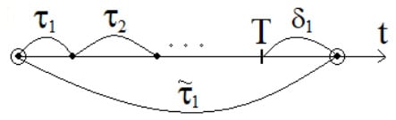
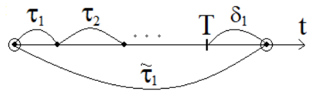
Let a recurrent flow J of points be given, defined by independent and identically distributed random variables (i.i.d.) Let denote the deterministic dead time, and, given the recurrent flow determine the recurrent flow of observed time instants (jumps). An observed instant of flow is the instant when the random walk jumps through fixed level T (see Figure 1). As an estimate of the parameter we consider , where i.i.d.v‘s. are the distances between adjacent points of the observed flow
Figure 1.
The first moment of the jump.
Remark 1.
In random walk theory are the step/jump increments, T is the fixed level/threshold, and is the overshoot.
Theorem 1.
If for some the function is positive, continuous and strictly monotonously decreasing, then is a consistent estimator of the parameter
Proof.
Since it follows that
Denote The overshoot of a random walk may begin at any point of the segment Therefore, regardless on the distribution of the initial overshoot point, the inequality
holds. And the function exists on the segment is continuous and is smaller than one, consequently Then Theorem 1 is proven. □
3. Deriving Recurrence Conditions for a Flow in the Simplest Case
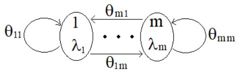
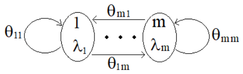
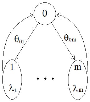
Consider a Poisson flow with a randomly varying intensity defined by a Markov chain with transition probabilities from state k to state . In the state k of the Markov chain , the process is at random time, distributed according to the exponential law with the parameter The moments at which these transitions occur correspond to the arrival times of new points in the flow J. Then the process instantly transitions into a state with probability . This section examines the simplest case (see Figure 2).
Figure 2.
Graph with initial transition probabilities.
For , the study [14] established conditions for the recurrence of a Markov arrival process (MAP) J, expressed in terms of the matrix . To achieve this, the joint probability density for a pair of successive inter-arrival times in the process J was calculated, and the conditions under which the equality holds referred to as the factorization conditions were determined. Distinct cases with exponential distributions and with mixtures of exponential distributions were identified, in which this factorization conditions are satisfied. Deriving the conditions for factorization proved to be quite complex and cumbersome even for , and it could not be carried out for .
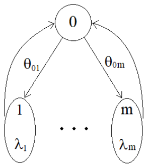
This raises the question how to modify the parameters of the flow J to render it recurrent in a simpler and more intuitive way. In this paper, we propose factorization conditions based on the assumption that the transition probabilities are independent of the first argument k. This conditions are equivalent to introducing a new state 0, and transforming the transition probability graph as shown in Figure 3. This approach yields a relatively simple conditions for the recurrence of the flow J. Furthermore, reaching state 0 serves as a regeneration point for the Markov chain , where . Consequently, for any , we obtain a condition for the recurrence of the flow J that is convenient to verify. This way of specifying factorization conditions can be extended, without significant difficulty, to more complex MAP models.
Figure 3.
Graph with transformed transition probabilities.
This construction is closely connected with a reset distribution after each arrival in [16].
4. Construction of an Estimate for Dead Time Based on a Flow of Observations and Establishment of Its Consistency
This simplification of the verification of recurrence for the flow J facilitates establishing the recurrence of the observation flow and constructing a consistent estimator . It should be noted that for and in the case when the distribution of the intervals between observations in the flow is exponential, and the estimate is a maximum-likelihood estimate.
Theorem 2.
If then and is a consistent estimator of the parameter
Proof.
Clearly, the intervals between the instants of occurrence of points in the random flow J are i.i.d.v‘s. with distribution
It is obvious that the function is positive and strictly monotonous decreasing. Then the consistency of the estimator of the parameter T follows from Theorem 1, since all its conditions are satisfied. In turn, for any
Theorem 2 is proven. □
Remark 2.
The following Monte-Carlo imitations have been made for N = 10,000. Here N is a number of realizations, each realization and
- If then and random variables are modeled for
- If then and random variables are modeled for
- If then and random variables are modeled for
- If then and random variables are modeled for
- If then and random variables are modeled for
- See Table 1.Table 1. Meanings of and
Remark 3.
It should be noted that the probability decreases with n as a geometric progression. This makes it possible to construct a confidence interval for T satisfying the condition
To obtain these results, precise knowledge of the MAP process parameters is not required. It suffices to have only constraints on MAP flow parameters.
- See Table 2.Table 2. Meanings of
For the simplest MAP flow the Ky Fan metric (see, for example [23,24])
It is worthy to note that for estimate considered in Remark 2 coincides with maximum likelihood estimator. If a deterministic T is replaced by a deterministic weakly perturbed T then an additional term is also included in the estimate .
5. The MAP Flow Model Defined by Erlang Distributions
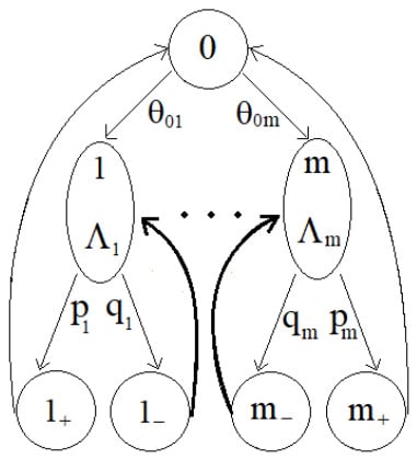
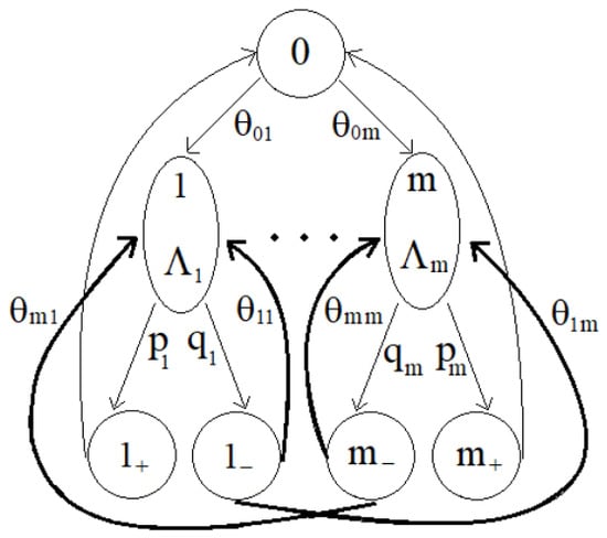
We now turn to a complication of model discussed in Section 4. Let the random time of a process in state k have a distribution tail Here is the appearance intensity of a new point of flow J, going from state k to state and from there to state 0, and is the intensity of getting from state k to state and from there to state k without getting to state 0 (see Figure 4).
Figure 4.
Graph of transition probabilities with thickened arrows from the substates .
Remark 4.
Since the Markov chain defining the MAP flow has regeneration points upon entering state 0 after which independent Poisson flows with parameters operate them the time intervals between the arrivals of new points in the flow J are also independent.
Remark 5.
The MAP flow model in Section 4 involves only a transition from state 0 to state k and a subsequent return to state 0 after a random time following an exponential distribution with parameter But In Section 5, two substates are introduced, and the Markov chain remains in a state k until it enters a sub state and, from there, transitions to state In this case, the interval between successive entries into the state follows an exponential distribution with parameter However, the transition to the state occurs after a random time following an exponential distribution with parameter . Then a new point in the MAP flow J appears.
Remark 6.
Lemma 1.
Assume that Figure 4 describes the Markov chain , which defines the MAP flow. Throughout the following, we assume Then the random variables are independent and .
Proof.
With probability , the chain enters state 0 (which corresponds to the appearance of a new moment in the flow J), and with probability it returns to state k. This cycle continues until enters state 0 for the first time (see Figure 4). The number cycles of the chain before returning to state 0 will determine the random time between points of the flow J, which has an Erlang distribution of order with density . We denote the tail of this distribution by and set .
The random variable is obvious to have an exponential distribution with parameter indeed,
Let us now calculate
This means that the random time spends in state k and the random variable , which determines the direction to state (to state ). Lemma 1 is proven. □
Theorem 3.
In conditions of Lemma 1 MAP flow defined by Erlang distributions the estimate of the parameter T is consistent.
Proof.
Let random variables and be independent and have exponential distributions with parameters Denote and set the Boolean random variable if , otherwise .
Denote thus, we can calculate the probabilities of the appearance of a new point in the flow J, taking into account the independence of random objects .
Here is the tail of the Erlang distribution of degree . The function is a functional series consisting of continuous functions. This series converges uniformly on , since the inequality
is satisfied. From the properties of uniform convergence of functional series it follows that is a continuous function on Since the functions are positive and strictly monotonous decreasing, the function also is positive and strictly monotonous decreasing on Then it follows the consistency of the estimate of the dead time T for the MAP flow from Theorem 1 determined by Erlang distributions. Theorem 3 is proven. □
6. Generalization of the MAP Flow Given by Erlang Distributions
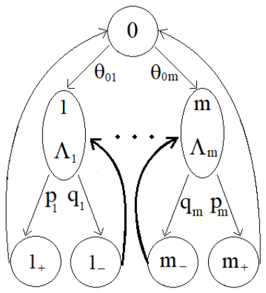
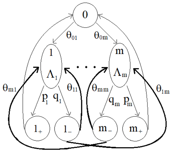
Let us generalize the model considered in Section 4. Let the Markov chain after being in state k instantly enters state with probability , and then enters state 0. Otherwise, the chain with probability instantly goes into state and from there into state with probability Here the transition probability matrix consists of non-negative elements, which add up to one in a row (see Figure 5).
Figure 5.
Graph of transition intensities for a generalized random flow model with thickened arrows from the substates .
Remark 7.
Theorem 4.
Assume that Figure 5 describes the Markov chain , which defines the MAP flow. Then for a generalized MAP flow, the estimate of the parameter T is consistent.
Proof.
Consider sequences consisting of numbers Then the Markov chain , controlling the random flow J, transits from state 0 to state with probability
Moreover, for any , the definition of the matrix and Lemma 1 implies the equality
Let us associate with each sequence of states of the Markov chain the sum of independent random variables with exponential distributions having parameters Then
From the last equality and Formula (1) we have
Consequently, the functional series consisting of continuous functions, converges uniformly on and therefore is continuous on this half-interval. Since the functions are positive and strictly monotonous decreasing, the function also is positive and decreasing on Then the statement of Theorem 4 follows from Theorem 1. Theorem 4 is proven. □
Theorem 5.
In terms and designations of Theorem 4 the following relations are true
Proof.
It is easy to obtain sequentially the following formulas
The statement of Theorem 5 is proven. □
Remark 8.
It should be noted that Theorem 5 defines the denominator of geometric progression of the upper bound for the sequence in Theorem 4. This proof requires a more careful examination of the monotonicity properties of the functions .
7. Conclusions and Discussion
A clear discussion of model limitations.
In this paper a concise summary of theoretical bounds and consistency properties of deterministic dead time T suggested estimate have been provided. These analyses were conducted under clearly specified conditions regarding the MAP (Markovian Arrival Process) that includes a reset distribution after each arrival. And the estimation of the deterministic dead time T is assumed as an absence of information about the MAP parameters. First condition allows for establishing the recurrence of the MAP flow J based on the regeneration ability of the Markov chain that controls it.
The second condition makes it possible to construct an estimate of the minimum distances between neighboring observations in the flow of observations without knowing its parameters. It complicates the construction of standard estimates for the parameter The rate of convergence of the estimate to the parameter T is investigated in terms of probability . It has been proven that this estimate is bounded by a decreasing geometric progression. Using the properties of functional series and the Weierstrass theorem on the maximum of a continuous function on a segment, inequalities are obtained for the tail of the distribution of a random jump through level T.
An upper bound for the common ratio of this progression is constructed. The paper also examines the issue how a perturbation in the deterministic parameter T affects the quality of the proposed estimate. The significance of this result lies in the fact that the exact calculation of the jump-size distribution for a random walk with is a computationally difficult task. For the simplest MAP flow confidence intervals have been calculated and the Ky Fan metric is estimated. The obtained analytical results were illustrated through a computational experiment.
Specific directions for future research.
It is necessary to spread numerical experiments for different partial models of MAP flow and for various values of the parameter n used to estimate the dead time T. It is also advisable to consider more complex MAP flows models with perturbed dead times. It is also of interest to examine a dead-time model with small random perturbations, both from a theoretical perspective and through computational experiments.
The research was carried out within the state assignment for IAM FEB RAS (N 075-00460-26-00).
Funding
This research received no external funding.
Data Availability Statement
The original contributions presented in this study are included in the article. Further inquiries can be directed to the corresponding author.
Conflicts of Interest
The author declares no conflict of interest.
References
- Albert, G.E.; Nelson, L. Contributions to the Statistical Theory of Counter Data. Ann. Math. Stat. 1953, 24, 9–22. [Google Scholar] [CrossRef] [Scilit]
- Meeks, C.; Siegel, P. Dead time correction via the time series. Am. J. Phys. 2008, 6, 589–590. [Google Scholar] [CrossRef] [Scilit]
- Basharin, G.P.; Gaidamaka, Y.V.; Samouylov, K.E. Mathematical theory of teletraffic and its application to the analysis of multiservice communication of next generation networks. Autom. Control. Comput. Sci. 2013, 47, 62–69. [Google Scholar] [CrossRef] [Scilit]
- Benali, A.; Peresan, A.; Varini, E.; Talbi, A. Modelling background seismicity components identified by nearest neighbour and stochastic declustering approaches: The case of Northeastern Italy. Stoch. Environ. Res. Risk Assess. 2020, 34, 775–791. [Google Scholar] [CrossRef] [Scilit]
- Naumov, V.; Gaidamaka, Y.; Yarkina, N.; Samouylov, K. Matrix and Analytical Methods for Performance Analysis of Telecommunication Systems, 1st ed.; Springer: Cham, Switzerland, 2021. [Google Scholar]
- Almousa, S.A.-D.; Horvath, G.; Telek, M. EM Based Parameter Estimation for Markov Modulated Fluid Arrival Processes. In Performance Engineering and Stochastic Modeling: 17-th European Workshop, EPEW 2021, and 26th International Conference, ASMTA 2021, Virtual Event, December 9–10 and December 13–14, 2021; Springer: Berlin/Heidelberg, Germany, 2021; pp. 226–242. [Google Scholar] [CrossRef] [Scilit]
- Bernal, M.G.; Lillo, R.E.; Ramirez-Cobo, P. Call center data modeling: A queueing science approach based on Markovian arrival process. Qual. Technol. Quant. Manag. 2025, 22, 631–658. [Google Scholar] [CrossRef] [Scilit]
- Gortsev, A.M.; Klimov, I.S. An estimate for intensity of Poisson flow of events under the condition of its partial missing. Radiotekhnika 1991, 12, 3–7. (In Russian) [Google Scholar]
- Gortsev, A.M.; Klimov, I.S. Estimation of the non-observability period and intensity of Poisson event flow. Radiotekhnika 1996, 2, 8–11. (In Russian) [Google Scholar]
- Gortsev, A.M.; Nezhelskaya, L.A. An asynchronous double stochastic flow with initiation of superfluous events. Discret. Math. Appl. 2011, 21, 283–290. [Google Scholar] [CrossRef] [Scilit]
- Kalyagin, A.A.; Nezhelskaya, L.A. Comparison of MP and MM estimates of the duration of dead time in a generalized semi-synchronous flow of events. Tomsk. State Univ. Bull. Manag. Comput. Sci. Inf. Technol. 2015, 3, 23–32. (In Russian) [Google Scholar] [CrossRef] [Scilit]
- Vetkina, A.; Nezhelskaya, L. Estimating the Distribution Parameter of Non-prolonging Random Dead Time Duration in Recurrent Semi-Synchronous Events Flow Through Maximum Likelihood. Lect. Notes Comput. Sci. 2024, 1423, 317–328. [Google Scholar] [CrossRef] [Scilit]
- Gortsev, A.M.; Vetkina, A.V. Application of the maximum likelihood method to estimate the uniform distribution parameter of the duration of non-extending dead time in a recurrent alternating semi-synchronous event flow. Tomsk. State Univ. Bull. Manag. Comput. Sci. Inf. Technol. 2023, 62, 36–49. (In Russian) [Google Scholar]
- Nezhelskaya, L.A. Joint probability density of the duration of intervals of a modulated MAP event flow and conditions for the recurrence of the flow. Tomsk. State Univ. Bull. Manag. Comput. Sci. Inf. Technol. 2015, 1, 57–67. (In Russian) [Google Scholar] [CrossRef] [Scilit]
- Borovkov, A.A. Probability Theory: Textbook; Springer: Berlin/Heidelberg, Germany, 2012. [Google Scholar]
- Nielsen, B.F. Note on the Markovian Arrival Process; 04141 Stochastic Processes; Danmarks Tekniske Universitet: Kongens Lyngby, Danmark, 1998; Volume 11. [Google Scholar]
- Smith, W.L. Regenerative Stochastic Processes. Proc. R. Soc. A Math. Phys. Eng. Sci. 1955, 232, 6-–31. [Google Scholar] [CrossRef] [Scilit]
- Haas, P.J. Regenerative Simulation: Stochastic Petri Nets: Springer Series in Operations Research and Financial Engineering; Springer: Berlin/Heidelberg, Germany, 2002; pp. 189–273. [Google Scholar] [CrossRef] [Scilit]
- Asmussen, S. Regenerative Processes. Applied Probability and Queues. Stoch. Model. Appl. Probab. 2003, 51, 168–185. [Google Scholar] [CrossRef] [Scilit]
- Sheldon, M.R. Introduction to Probability Models (9th Edition): Textbook; University of California, USA: Oakland, CA, USA, 2007. [Google Scholar]
- Lotov, V.I.; Tarasenko, A.S. On the distribution of the first exit time and overshoot in a two-sided boundary crossing problem. Sib. Adv. Math. 2013, 23, 91–98. [Google Scholar] [CrossRef] [Scilit]
- Lotov, V.I. Factorization method in boundary crossing problems for random walks. Markov Process. Relat. Fields 2019, 25, 709–722. [Google Scholar]
- Fan, K. Entfernung zweier zufalliger Großen und die Konvergenz nach Wahrscheinlichkeit. Math. Z. 1944, 49, 681–683. [Google Scholar] [CrossRef] [Scilit]
- Zolotarev, V.M. Modern Theory of Summation of Random Variables; Modern Probability and Statistics; VSP: Utrecht, The Netherlands, 1997. [Google Scholar]

Disclaimer/Publisher’s Note: The statements, opinions and data contained in all publications are solely those of the individual author(s) and contributor(s) and not of MDPI and/or the editor(s). MDPI and/or the editor(s) disclaim responsibility for any injury to people or property resulting from any ideas, methods, instructions or products referred to in the content. |
© 2026 by the author. Licensee MDPI, Basel, Switzerland. This article is an open access article distributed under the terms and conditions of the Creative Commons Attribution (CC BY) license.