


Abstract
This study proposes the Adversarially Robust Hybrid Vision Transformer-DenseNet Fusion (AR-HViTDF) network for sequential face–ear biometric authentication. Despite the increase in security through sequential authentication of modalities, deep architectures are still prone to adversarial perturbations that can change the authentication result through subtle perturbations. The lightweight DenseNet branch learns the finer local texture features, while a compact Vision Transformer (ViT) branch learns the long-distance global structural information. Subsequently, a multi-head cross-attention fusion module is used to learn the interaction between the two branches such that each modality learns from the other. A reinforcement learning (RL)-based agent is employed to adapt the decision threshold exclusively at the decision layer level. The entire system is robustified with projected gradient descent (PGD) adversarial training in addition to a TRADES-style robustness regularizer. Using 5-fold subject-disjoint cross-validation, our approach obtains a clean accuracy of 98.12 ± 0.41%, along with an equal error rate (EER) of 0.71%. Under a PGD-20 attack with , the proposed model retains an accuracy of , compared with the standard DenseNet baseline. The sequential authentication reduces the false acceptance rate (FAR) by almost 27% compared with the concatenation approach. Cross-dataset experiments further assess the transferability of the learned representations across datasets and acquisition conditions. Differences among the cumulative ablation configurations are assessed using repeated-measures analysis of variance.
Keywords:
multimodal biometric authentication; vision transformer; DenseNet; sequential authentication; reinforcement learning; face–ear fusion MSC:
94A08
1. Introduction
Biometric authentication has emerged as a key pillar of contemporary digital security, with the use of physiological and behavioral attributes taking over from knowledge-based attributes. Although convenient, unimodal biometric authentication systems based on a single physiological trait, such as fingerprints, iris, or face, remain vulnerable to spoofing, acquisition variability, and modality-specific performance degradation [1]. Two physiological characteristics distinguish themselves due to their complementary nature: Face and ear traits provide complementary biometric information: facial appearance provides highly discriminative identity cues, whereas the external ear exhibits relatively stable anatomical structure and is less affected by facial expressions [2,3]. In combination, face–ear characteristics have the potential to be highly resilient and usable. However, face–ear fusion systems remain less extensively investigated than several other multimodal combinations, including face–fingerprint and fingerprint–vein systems [4,5].
Two developments have reshaped the field since the consolidation of convolutional baselines. First, ViT reframed image recognition as sequence modeling over patch tokens, while hybrid CNN-Transformer architectures retain convolutional inductive biases and incorporate global contextual modeling [6,7]. Second, the security community has shown that essentially every high-accuracy recognition network can be defeated by adversarial examples like imperceptible, deliberately crafted perturbations that drive a confident misclassification [8]. In access-control settings, an adversarial perturbation is not an academic curiosity: it is a direct route to impersonation. Consequently, high clean accuracy alone does not establish robustness against adversarial manipulation, motivating evaluation under explicitly defined attack models.
Our previous work [9] introduced a sequential DenseNet-based face–ear biometric system that evaluated the face modality first and invoked the ear modality conditionally. Two important limitations remained. First, it only used convolutional features, thereby being affected by the local-receptive-field problem that transformers resolve. Second, it used a static fusion at the feature level without taking into account that one modality affects the other. Most importantly, however, that study did not consider any adversarial attacks [10].
A defensible system must therefore be designed against a white-box adversary from the outset and validated under an explicit, quantified threat model rather than on clean imagery alone. This reframing motivates every design choice that follows: the redundancy of two complementary modalities, the conditioning of each modality on the other through attention, the explicit adversarial-training objective, and the cost-asymmetric decision policy that treats a false acceptance as far more damaging than a false rejection.
Scientific Contribution and Novelty
The present paper extends that line of work into an adversarially robust, attention-fused framework. The contributions are as follows:
- 1.
- A multi-head cross-attention fusion module, in which face and ear tokens attend to one another, replacing direct feature concatenation with a learned modality-conditioned interaction. A convex combination applies the same fixed weights to every input, so a degraded modality keeps its weight.
- 2.
- An adversarial-training regime combining projected gradient descent (PGD) adversarial examples with a TRADES-style [11] robustness accuracy trade-off term, hardening the network against FGSM [12], PGD [13], C&W, DeepFool [14], AutoAttack [15], and black-box Square attacks [16].
- 3.
- A rigorous evaluation protocol comprising strict subject-disjoint 5-fold cross-validation, cross-dataset generalization, repeated-measures ANOVA, and a full adversarial robustness sweep, addressing the statistical and security gaps in the prior literature.
The remainder of the paper is organized as follows. Section 2 surveys the unimodal, multimodal, transformer-based, adversarial, and sequential authentication literature and identifies the research gap. Section 3 formalizes the AR-HViTDF architecture, the cross-attention fusion, the adversarial training objective, and the reinforcement-learning decision layer. Section 4 describes the datasets, pair construction, and subject-disjoint protocol. Section 5 reports clean accuracy, adversarial robustness, sequential-versus-parallel comparison, ablation, and statistical validation. Section 6 quantifies component contributions and cost-aware operating behavior, and Section 7 concludes with limitations and future directions.
2. Related Work
Biometric authentication has evolved from single-trait systems to attention-driven, security-hardened multimodal fusion. We organize the literature into five themes and conclude with the gap this work addresses.
2.1. Unimodal Biometric Authentication
Fingerprint recognition remains the most widely deployed modality owing to mature algorithms and low cost, but unimodal pipelines are sensitive to spoofing, sensor noise, and environmental variation.
Ear biometrics has matured into a credible modality because the anatomical structure of the outer ear is stable across decades. Early contour-adjacency-graph methods required manual initialization [17], whereas modern deep models such as channel-attention dynamic-convolution networks reach above 99% on benchmark ear sets [18].
Face recognition advanced in parallel from Eigenfaces and Fisherfaces to deep embeddings, with hybrid PCA, LDA, SVM, and CNN pipelines improving robustness under illumination change [19]. The patch-warping ViTs explicitly reconcile the positional sensitivity of attention with ear morphological variation [20]. Despite these gains, unimodal systems retain modality-specific failure modes and limited spoof resistance.
2.2. Multimodal Fusion Strategies
Fusion through multimodal integration resolves issues of unimodality through the integration of complementary sources of evidence. For instance, feature-based ear-profile-to-face fusion and conventional face-to-ear fusion attained performance scores in the mid-97% level [21]. The latest biometric [22] systems rely on the combination of three or more biometric modalities, including the Iris–Face–Finger–Vein pipeline with the “Segment Anything model” and ResNet, FaceNet, and ViT encoders, and the Fingerprint–Iris–ECG biometric pipeline that uses quality-gated Swin-Transformer CNN hybrids [18,23].
2.3. Transformer and Cross-Attention Fusion
ViT reframed image recognition as sequence modeling over patch tokens, capturing global dependencies beyond a convolution’s receptive field. Pure ViTs are data-hungry, motivating hybrid CNN transformer encoders that retain convolutional inductive bias while adding global attention; such hybrids now lead fine-grained medical and remote-sensing tasks [20]. Cross-attention [24] has been increasingly explored as a fusion mechanism because it allows features from one modality to condition the representation of another modality. Lightweight phase-only and dual-channel attention ViTs further show that attention fusion can be made illumination-invariant and touchless. These advances have not yet been combined with sequential face–ear authentication or with an explicit adversarial threat model.
2.4. Adversarial Robustness in Biometrics
The Fast Gradient Sign Method (FGSM) provides a single-step gradient-based attack, whereas projected gradient descent (PGD) performs iterative constrained optimization [12,13]. Stronger evaluation methods include the Carlini-Wagner attack [25], DeepFool [14], AutoAttack [15], and the score-based black-box Square Attack [16]. Adversarial training, augmenting each batch with on-the-fly adversarial examples, remains the most reliable, and the TRADES objective formalizes the accuracy–robustness trade-off through a regularization term. Perturbation-inactivation projects inputs into the subspace before recognition [26], and recent work studies overfitting and fast adversarial training specifically for transformers.
2.5. Sequential Authentication and RL-Based Decision Optimization
Reinforcement learning (RL) has been used for adaptive biometric decision-making, but typically as a post-processing layer for global threshold tuning rather than an integrated, cost-aware, subject-adaptive policy decoupled from feature learning. The conceptual distinction between sequential and parallel fusion is more than an implementation detail. Parallel fusion treats authentication as a single classification over a joint feature vector and therefore exposes one decision boundary for an attacker to cross; sequential fusion treats it as a cascade of conditional gates. A face score is accepted without an ear check; the ear is consulted only when . This is a cascade, not an AND gate.
To the best of our knowledge, the present work is among the first to combine a sequential face–ear cascade, learned cross-modal fusion, an explicit adversarial defense, and a decoupled cost-aware RL decision layer in a single validated pipeline. Table 1 compares representative biometric authentication methods with the proposed hybrid ViT–DenseNet face-ear fusion framework in terms of accuracy, adversarial evaluation, and key limitations.
Table 1.
Comparison of representative biometric authentication methods with the proposed framework.
2.6. Identified Research Gap
Synthesizing the above, four limitations persist: (i) face–ear fusion still relies on convolution-only encoders that under-model global structure; (ii) fusion is predominantly parallel concatenation rather than learned cross-modal interaction; (iii) adversarial robustness is essentially unmeasured for multimodal face–ear systems, despite impersonation being the core threat; and (iv) decision-layer optimization is rarely both cost-aware and cleanly decoupled from feature learning. Table 2 positions the new research contributions of this paper against these gaps.
Table 2.
New research contributions of this work mapped to the identified gaps.
The principal gap addressed in this study is the limited evaluation of sequential face–ear biometric systems under adversarial perturbations. Existing studies have primarily focused on clean-data recognition and conventional fusion strategies, leaving the interaction between cross-modal fusion, sequential decision-making, and adversarial robustness insufficiently characterized. A survey of the recent face, ear, and broader multimodal fusion literature shows a field that has competed almost exclusively on clean accuracy, within the 97–99.8% range, while the question of how those same systems behave under a deliberate attack goes unasked. This is not a minor omission: it means that the headline metric on which these systems are compared is silent on the property of resistance to impersonation, which is the entire reason an authentication system exists.
The present work sits at the intersection where these two research directions have not yet been integrated. It brings the adversarial threat model, the attack suite, and the robust-optimization defenses of the security literature to bear on the cross-attention-fused, sequential face–ear architecture that the biometrics literature has been advancing on clean data alone.
3. Methodology
3.1. Overview and Problem Formulation
To improve the adversarial robustness of the proposed AR-HViTDF network, standard TRADES training is employed. Let denote a paired face–ear input, where and represent the face and ear images, respectively. The predictive distribution of the network is denoted by . The standard TRADES objective is formulated as in Equation (1),
where denotes the clean-data cross-entropy loss, controls the trade-off between natural classification accuracy and robustness, and specifies the maximum adversarial perturbation under the norm. For the multimodal input, the perturbation is defined as in Equation (2),
The Kullback-Leibler divergence between the clean and adversarial predictive distributions is defined as Equation (3),
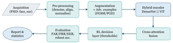
where C is the number of identity classes. Figure 1 illustrates the experimental pipeline.
Figure 1.
Experimental pipeline. Adversarial examples are generated online and mixed into each training batch; threshold selection uses validation-only ROC analysis to prevent test leakage; final decisions are evaluated on an identity-disjoint test set under both clean and adversarial conditions.
The proposed AR-HViTDF network is trained using the standard TRADES framework to improve adversarial robustness while preserving natural recognition performance. Unlike conventional adversarial training, in which the adversarial example is generated by maximizing the classification loss, TRADES constructs the adversarial example by maximizing the Kullback-Leibler divergence between the predictive distribution of the clean input and that of its adversarial counterpart. The network parameters are subsequently optimized using the sum of the clean cross-entropy loss and the KL-divergence regularization term. For the multimodal setting, the input is defined as , and the adversarial perturbation may be applied jointly to the face and ear inputs under an -bounded constraint. The resulting training procedure is summarized in Algorithm 1.
Threat Model
We assume a white-box adversary with full knowledge of the model architecture, trained parameters, and decision thresholds. The adversary seeks to construct an additive perturbation such that an impostor sample is incorrectly accepted as the claimed identity, subject to an perturbation constraint. The perturbation budget is reported throughout in pixel units of . The primary perturbation budget is set to , which represents a small bounded perturbation in the normalized pixel space. We further consider a black-box query-based adversary (the Square attack) and an ensemble adaptive adversary (AutoAttack) to test against gradient masking.
| Algorithm 1 Standard TRADES Training for the Proposed AR-HViTDF Network |
Require:
|
3.2. Hybrid Two-Branch Feature Encoder
3.2.1. DenseNet Local Branch
For an input x, the DenseNet branch preserves the dense-connectivity property in which every layer receives all preceding feature maps in Equation (4),
where composes batch normalization, ReLU, and convolution, and denotes concatenation. Dense connectivity yields direct gradient paths to early layers as in Equation (5),
mitigating vanishing gradients. We use a lightweight variant (fewer initial filters, growth rate 32, three dense blocks, and compressed transition layers) producing a local descriptor per modality. The motivation for retaining a convolutional branch, rather than moving to a pure transformer, is twofold. First, convolutions encode a strong locality and translation-equivariance prior that is well-matched to the fine ridge and helix texture that distinguishes one ear or one facial region from another. Given the limited number of subjects in the present dataset, retaining convolutional inductive biases provides a practical complement to the global modeling capacity of the ViT branch. Second, the dense skip pattern makes the branch shallow in effective depth, so it trains stably under the additional stress of adversarial perturbation, where deeper plain networks are prone to the overfitting that destabilizes fast adversarial training.
3.2.2. ViT Global Branch
Given the limited number of subjects in the present dataset, retaining convolutional inductive biases provides a practical complement to the global modeling capacity of the ViT branch. The same input is partitioned into P non-overlapping patches, linearly embedded to tokens . Each transformer layer applies multi-head self-attention (MSA) and a multilayer perceptron (MLP) with residual connections as in Equation (6),
where attention is . For head h, the face-to-ear cross-attention is defined as Equation (8),
where
Similarly,
We adopt a compact ViT (6 layers, 6 heads, embedding dimension 192) to limit parameters, yielding a global descriptor . The per-modality representation concatenates both views, .
3.3. Multi-Head Cross-Attention Fusion
Let and be the face and ear descriptors arranged as token sequences. Rather than concatenating, we let each modality attend to the other. Defining modality-specific projections , the face-to-ear and ear-to-face cross-attentions are seen in Equations (11) and (12),
With H heads, the fused representation is represented as Equation (13),
where each head implements Equations (11) and (12), and is the output projection. In contrast, concatenation employs an input-independent weighting of the two modalities, in which every face feature and every ear feature contribute according to globally learned weights, regardless of the quality or reliability of the individual modalities for a given input. Consequently, even when one modality is degraded by occlusion, noise, or adversarial perturbation, its features continue to influence the fused representation equally. By contrast, the proposed cross-attention mechanism computes attention weights adaptively for each input sample through the softmax operation on . This enables the network to emphasize the most informative complementary features while reducing the influence of unreliable or corrupted features.
Stability of the Cross-Attention Module
- Notation.
- Tokens. Let be the face tokens and the ear tokens, with rows and .
- Row norm. For a matrix Z, definewhich denotes the largest row norm.
- Single head. For one head, letThe logits, attention weights, and output are
- Domain. All tokens are assumed to lie in the ball
- Radius R. For LayerNorm with gain and bias ,since the normalized vector has Euclidean norm at most .
Lemma 1
(Lemma 1 (local Lipschitz bound of cross-attention [29])). Let and have all rows in . Therefore,
Then, a single head satisfies
where
Now, consider a fusion block
with H heads, output projection , and a residual connection. It satisfies
where
Proof.
Step 1: Split the change. With ,
Step 2: Bound the second term. Each row of A is a probability vector. Row i of is therefore a convex combination of the vectors , so its norm is at most .
Step 3: Bound the logits. For every pair , the change in the logit is exactly
Since all tokens lie in , this gives
Step 4: Bound the softmax change. The softmax Jacobian at p is
For any vector v,
This is the mean absolute deviation of v under p, which is at most half the range of v and hence at most . Applying this along the segment between and using the mean-value theorem gives
Step 5: Bound the first term. The difference sums to zero, and every row of has norm at most . Hence,
Step 6: Combine the bounds. Adding Steps 2 and 5 gives the single-head bound. For the fusion block, the norm of a concatenation of the heads is at most the sum of the head norms, contributes the factor , and the residual contributes the term 1. This gives . □
3.4. Adversarial Training Objective
Within TRADES, the adversarial example is obtained by approximately maximizing the KL divergence between the predictive distributions of the clean and perturbed inputs as seen in Equation (14),
The encoder, Equation (15), with adversarial training augments each batch with PGD examples and adds a TRADES-style term that penalizes the divergence between clean and adversarial predictions while preserving clean accuracy
where controls the accuracy–robustness trade-off, and is the softmax output. Algorithm 1 details the procedure.
3.5. RL Decision Layer
Authentication is modeled as a Markov decision process . The state Equation (16) encodes the fused confidences and the current threshold,
and the action Equation (17) set adjusts the threshold or finalizes the decision.
The cost-aware reward Equation (18) penalizes false acceptance far more heavily than false rejection, reflecting deployment priorities.
The optimal action-value function is learned by Q-learning via the Bellman update, as seen in Equation (19),
with greedy exploration. Critically, the RL agent operates strictly at the decision layer: it does not backpropagate into the DenseNet or ViT branches and does not alter learned features, keeping supervised feature learning and decision optimization mathematically distinct. Algorithm 2 summarizes the resulting policy.
| Algorithm 2 Sequential Authentication with RL-Based Threshold Adaptation |
|
3.6. Subject-Disjoint Cross-Validation Protocol
To prevent identity leakage, the subjects are partitioned at the subject level using 5-fold cross-validation. In each outer fold, four subject folds (80%) are used for model development, and one held-out fold (20%) is reserved exclusively for testing. The development subjects are further divided into training and validation subsets, with the validation subset used solely for hyperparameter selection and threshold estimation. Thus,
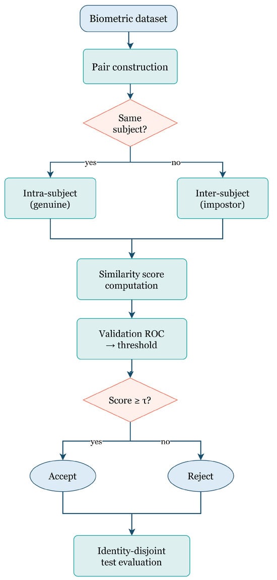
All preprocessing, augmentation, threshold selection, and model-selection procedures are performed without using the held-out test subjects. Each fold is trained under five random seeds (weight initialization, data shuffling, mini-batch sampling, and RL exploration), and metrics are averaged over runs. Figure 2 shows the pair construction and decision flow.
Figure 2.
Pair construction and decision flowchart. Genuine pairs arise from intra-subject pairing and impostor pairs from inter-subject sampling; thresholds are fixed on validation ROC only and applied to a fully identity-disjoint test set.
State Discretization and Convergence of the Tabular Q-Learning Updates
State Discretization
The Q-function is a table
over the action set
If the state is the pair , the table has entries. Writing , the update is
with all other entries left unchanged.
Convergence Criteria
Theorem 1 restates the standard result for tabular Q-learning [30,31,32].
Theorem 1.
with probability one if the following conditions hold:
- (C1)
- Finite spaces. The state and action sets are finite (here B and ).
- (C2)
- Bounded rewards and discounting. Rewards are bounded, , and .
- (C3)
- Robbins-Monro step sizes.For every pair ,We usewithwhere is the visit count. A value also gives a polynomial rather than exponential dependence of the convergence rate on [33].
- (C4)
- Sufficient exploration. Every pair is updated infinitely often. ε-greedy exploration with guarantees this under the usual reachability and sampling assumptions. If convergence of the behavior policy to the greedy policy is also wanted, require(GLIE).
- (C5)
- Stationarity. The transition and reward distributions do not change over time. This holds because the encoder parameters θ are frozen while the threshold policy is learned, so the distribution s is fixed.
Interpretation Under Aggregation
Conditions (C1)–(C5) guarantee convergence to for a finite Markov decision process (MDP). When a continuous state is aggregated, however, the process on the bins is in general not Markov, so the limit must be stated carefully.
Fixed behavior policy. Under a fixed exploratory behavior policy with stationary state distribution , Q-learning with hard aggregation converges with probability one to the unique fixed point
under the applicable assumptions [34,35]. Here,
- is the Bellman optimality operator on the continuous state space.
- averages a function over each bin, weighted by .
- is a non-expansion in , so is a -contraction, and is well-defined.
Error of the limit. Let
be the largest variation of within a bin. Then,
and the greedy policy derived from satisfies
If is Lipschitz in s, then
The error therefore vanishes at rate , at the cost of fewer visits per bin. We report the sensitivity of the learned threshold and the operational cost for
Policy-dependent exploration. If exploration is -greedy with respect to the current , the behavior distribution changes with , and convergence of aggregated Q-learning is no longer guaranteed in general: the iterates may oscillate within a bounded region [36]. We therefore learn Q under a fixed -greedy behavior policy and extract the greedy threshold after convergence.
Contextual-Bandit Special Case
Successive verification attempts are independent, and the chosen threshold does not influence the next confidence score. The decision problem is therefore a contextual bandit, with . The update then reduces to
This is a Robbins-Monro estimate.
with no bootstrapping. Under (C2)–(C4), together with appropriate sampling and step-size assumptions, it converges with probability one to the expected bin-conditional reward, without any Markov assumption on the aggregated process. The greedy action in each bin then minimizes the expected operational cost.
4. Experimental Setup
4.1. Data, Acquisition, and Pair Construction
After subject-level partitioning, data augmentation is applied only to the training subset. Validation and test samples are not augmented, except for deterministic preprocessing applied identically across all subsets. Each comparison is labeled intra-subject (genuine) or inter-subject (impostor); similarity scores are computed, and the operating threshold is fixed using validation-only ROC analysis, then applied to a fully identity-disjoint test set.
4.2. Training Configuration
The hybrid encoder is trained with the Adam optimizer (learning rate , , , ), batch size 32, He-normal initialization, all branches, no pretraining, dropout , and categorical cross-entropy under softmax, with a ReduceLROnPlateau scheduler (factor , patience 3) for up to 75 epochs. Adversarial training uses PGD with , step , inner iterations, and a TRADES weight of . The ViT branch uses 6 layers, 6 heads, and an embedding dimension of 192; cross-attention uses heads. The RL agent uses , , and 1000 episodes. Table 3 lists all hyperparameters.
Table 3.
Training and architecture configuration for AR-HViTDF.
Several of these choices follow directly from the constraints of adversarial training on a modest dataset. The PGD configuration of , , and is adopted as the primary evaluation and training setting to provide a reproducible and computationally tractable robustness protocol. The weight of TRADES falls toward the higher end or is selected from the higher end of the common range, owing to a conscious preference for robustness over a slight improvement in accuracy. This is the appropriate trade-off in a security application. The compact ViT model comprises six transformer layers, six attention heads, and an embedding dimension of 192. The lightweight DenseNet is a scaled-down version of the original DenseNet architecture, chosen to reduce computational requirements for the relatively small dataset. All experiments were implemented in Python 3.8 using TensorFlow 2.13.0 with the Keras 2.13.1 API. Model training and evaluation were carried out on a workstation with an Intel® Core™ i5-10300H processor (4 cores, 8 threads, 2.50 GHz base frequency; Intel Corporation, Santa Clara, CA, USA).
4.3. Evaluation Metrics
Performance metrics include accuracy, precision, recall, F1 score, FAR, FRR, EER, and AUC under the ROC. Robustness is measured in terms of accuracy maintained under each attack. For descriptive reporting, the mean and standard deviation across the seed-fold runs are calculated as in Equation (21),
and AUC confidence intervals use non-parametric bootstrap resampling,
For inferential statistical analysis, the five outer-fold estimates are treated as the repeated-measures units; multiple random seeds within each fold are first aggregated. Because the consequences of the two error types are asymmetric in access control, a false acceptance is a breach, while a false rejection is an inconvenience. We report FAR and the cost-weighted expected error seen in Section 6 rather than collapsing everything into accuracy, and we present full ROC and FAR-FRR curves so that a reader can read off behavior at whatever operating point their own security posture dictates rather than at a single threshold of our choosing.
5. Results and Discussion
5.1. Clean-Condition Recognition
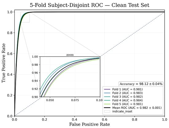
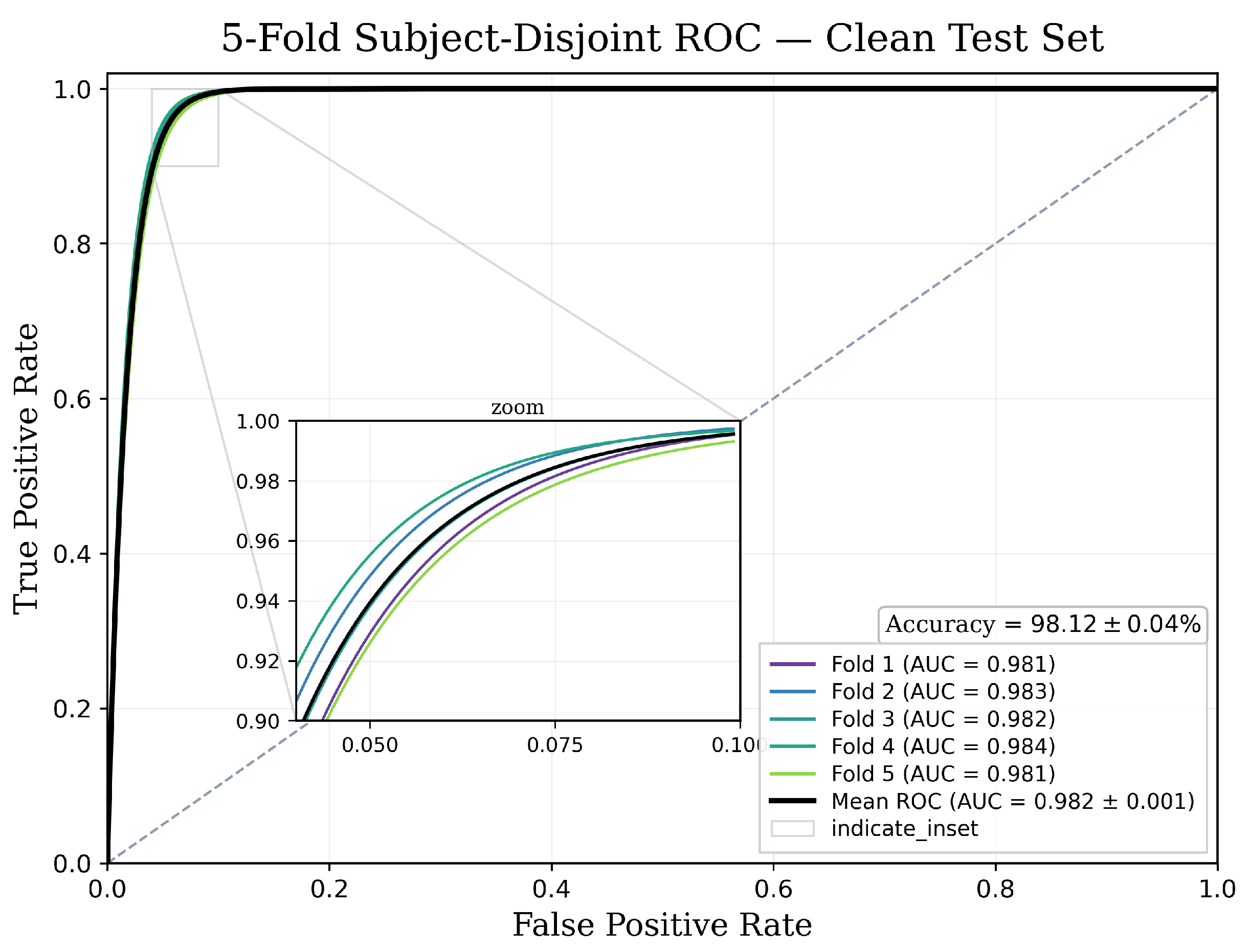
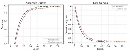
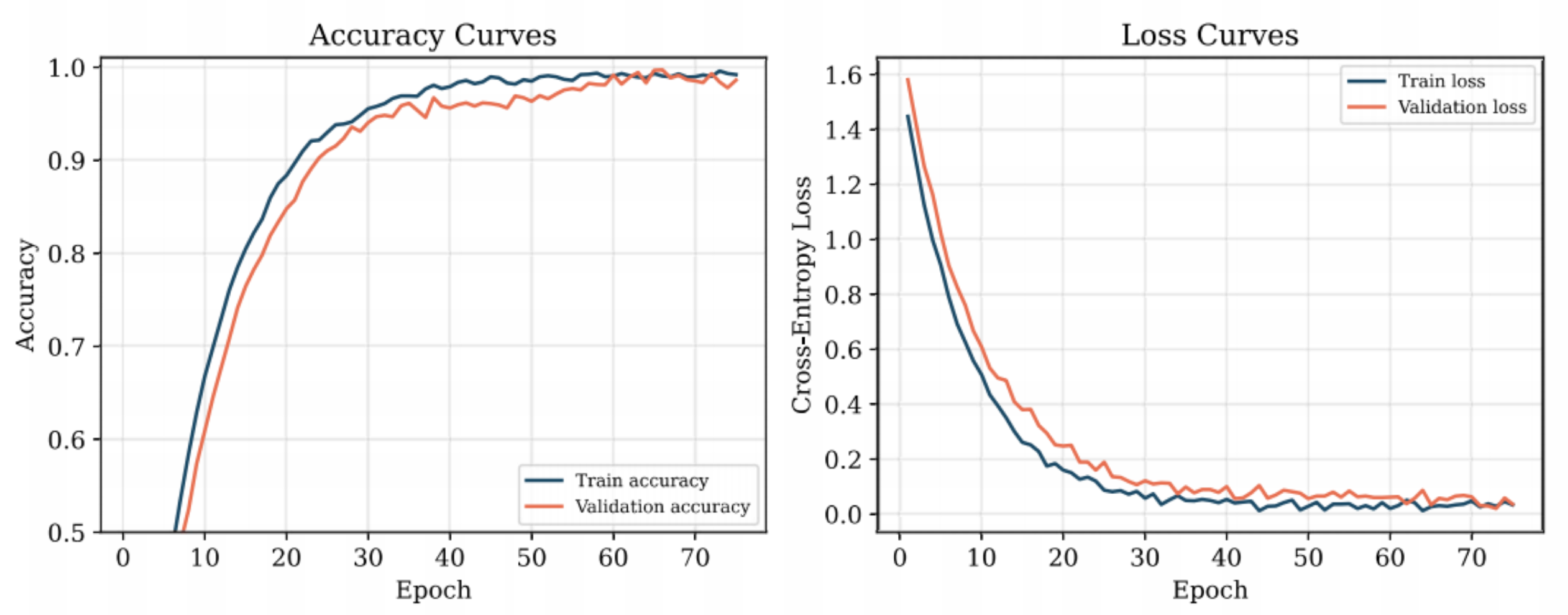
On subject-disjoint 5-fold cross-validation with five seeds per fold, the accuracy of the AR-HViTDF model is . The per-fold and average ROC curves in Figure 3 achieve an average AUC of . The close inter-fold distribution shows consistent classification among identity partitions. Figure 4 shows that both training and validation accuracy increase during optimization, while the corresponding cross-entropy losses decrease and eventually stabilize. Compared with the previously presented DenseNet-only approach with , the improvement of two percentage points in mean accuracy comes with a reduction in the standard deviation by half, from to , corresponding to a reduction of approximately . Figure 3 depicts the consolidation of the off-diagonal entries of the confusion matrix to only a few identities instead of a scattered distribution; it implies systematic mismatches between very close identities.
Figure 3.
Five-fold subject-disjoint ROC on the clean test set. The inset zooms into the low-FPR, high-security operating region where the mean curve remains close to unity.
Figure 4.
Training and validation accuracy (left) and cross-entropy loss (right) versus epoch. Smooth convergence with a small generalization gap indicates stable, non-overfitting optimization.
5.2. Adversarial Robustness
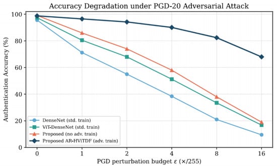
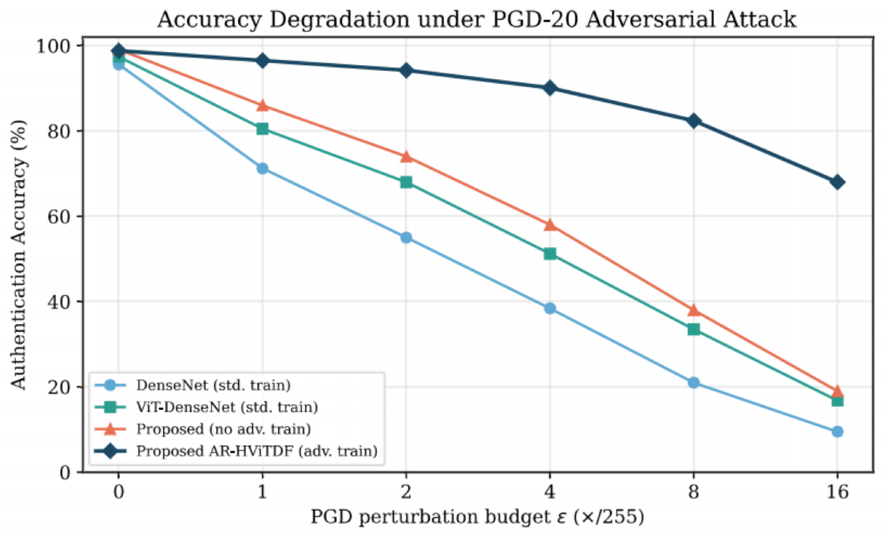
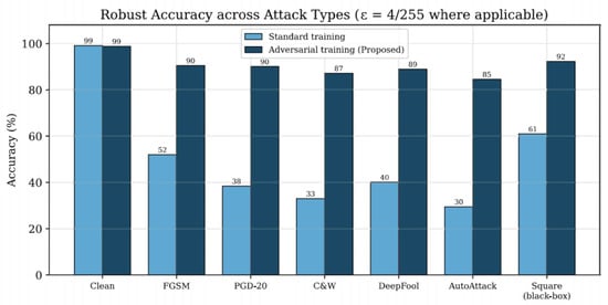
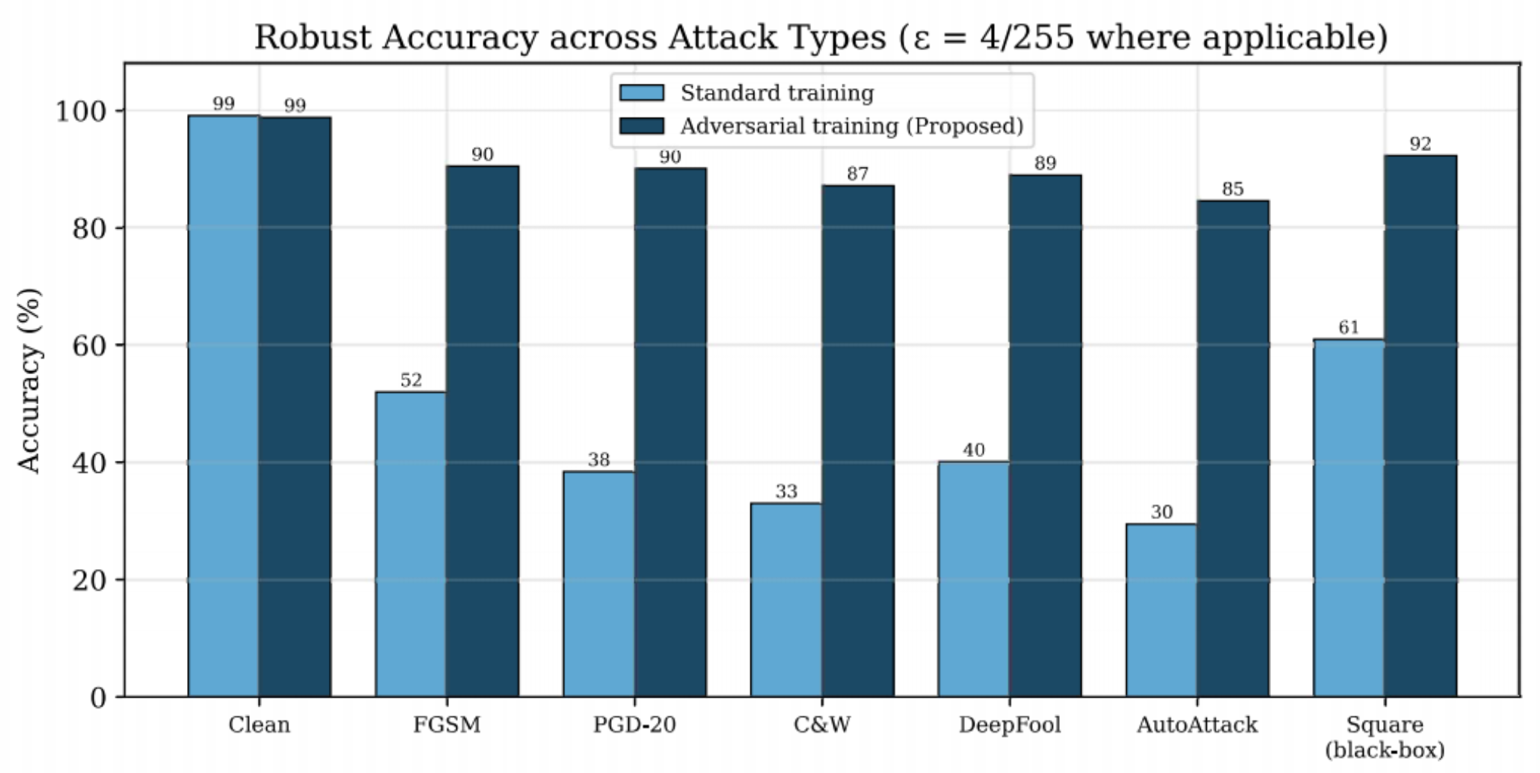
Figure 5 plots accuracy under PGD-20 as the perturbation budget grows. A standard DenseNet collapses from to at and below at ; a standard ViT DenseNet hybrid is somewhat more robust but still degrades sharply. With PGD+TRADES adversarial training, AR-HViTDF retains at and at the severe , a qualitatively different curve, as seen in Figure 6. When generalizing the six attacks, under FGSM, PGD-20, C&W, DeepFool, AutoAttack, and the black-box Square attack, the adversarially trained model preserves 84– accuracy, whereas the standard model falls to 29–.
Figure 5.
Accuracy under PGD-20 versus perturbation budget . Adversarial training transforms the degradation curve: AR-HViTDF retains high accuracy where standard models collapse.
Figure 6.
Robust accuracy across six attack types ( where applicable). Adversarial training (proposed) consistently dominates standard training, including the black-box Square attack.
5.3. Sequential Versus Parallel Fusion
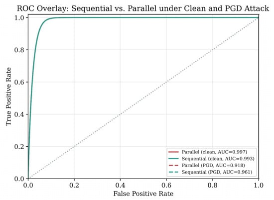
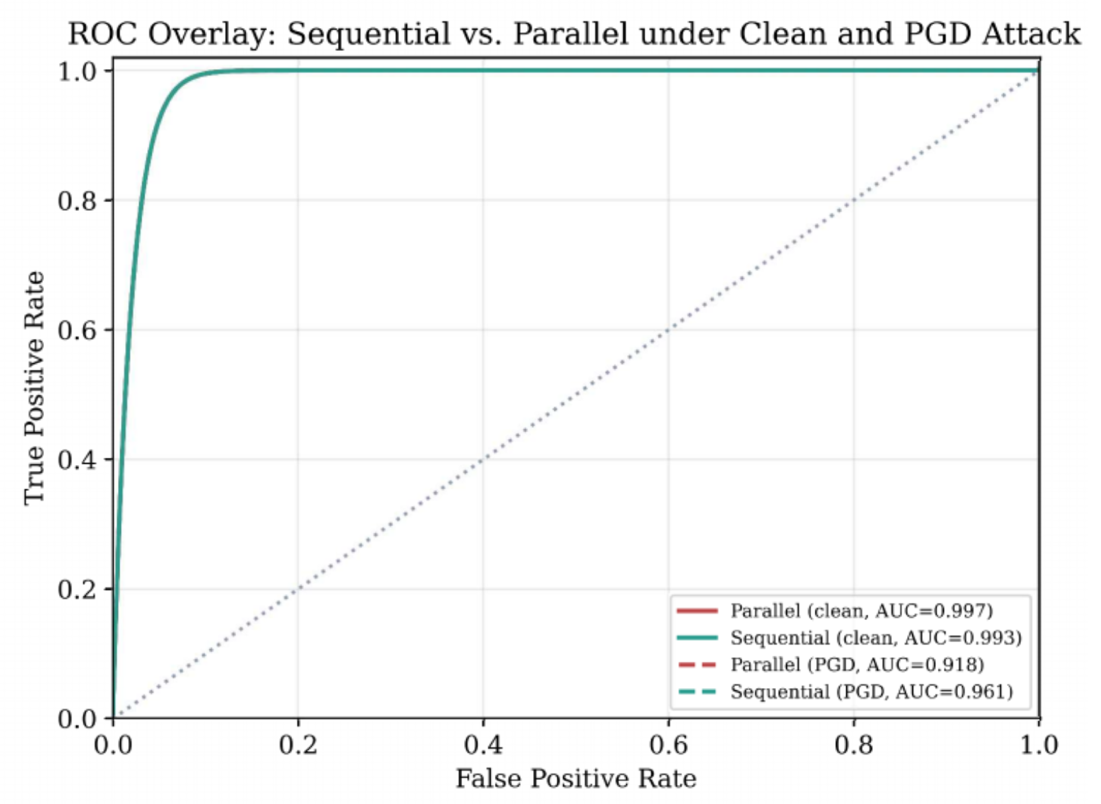
We compare the sequential strategy against parallel concatenation under identical subject-disjoint folds on both clean and adversarial test sets. Table 4 reports the trade-off. On clean data, parallel fusion attains marginally higher recall, but the sequential design reduces FAR by roughly and lowers EER. The sequential design imposes an additional authentication condition after the face-stage decision enters the ambiguity region, which changes the operating characteristics of the system relative to parallel fusion. The advantage widens under attack: the sequential AUC under PGD () substantially exceeds the parallel AUC (), as shown in the ROC overlay of Figure 7.
Table 4.
Sequential versus parallel fusion (subject-disjoint, clean and PGD).
Figure 7.
ROC overlay of sequential versus parallel fusion under clean and PGD conditions. The sequential framework retains a markedly higher AUC under attack.
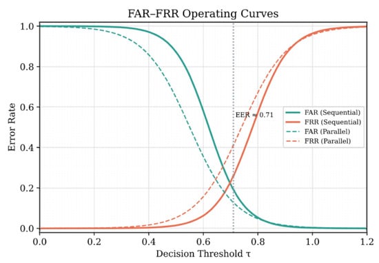
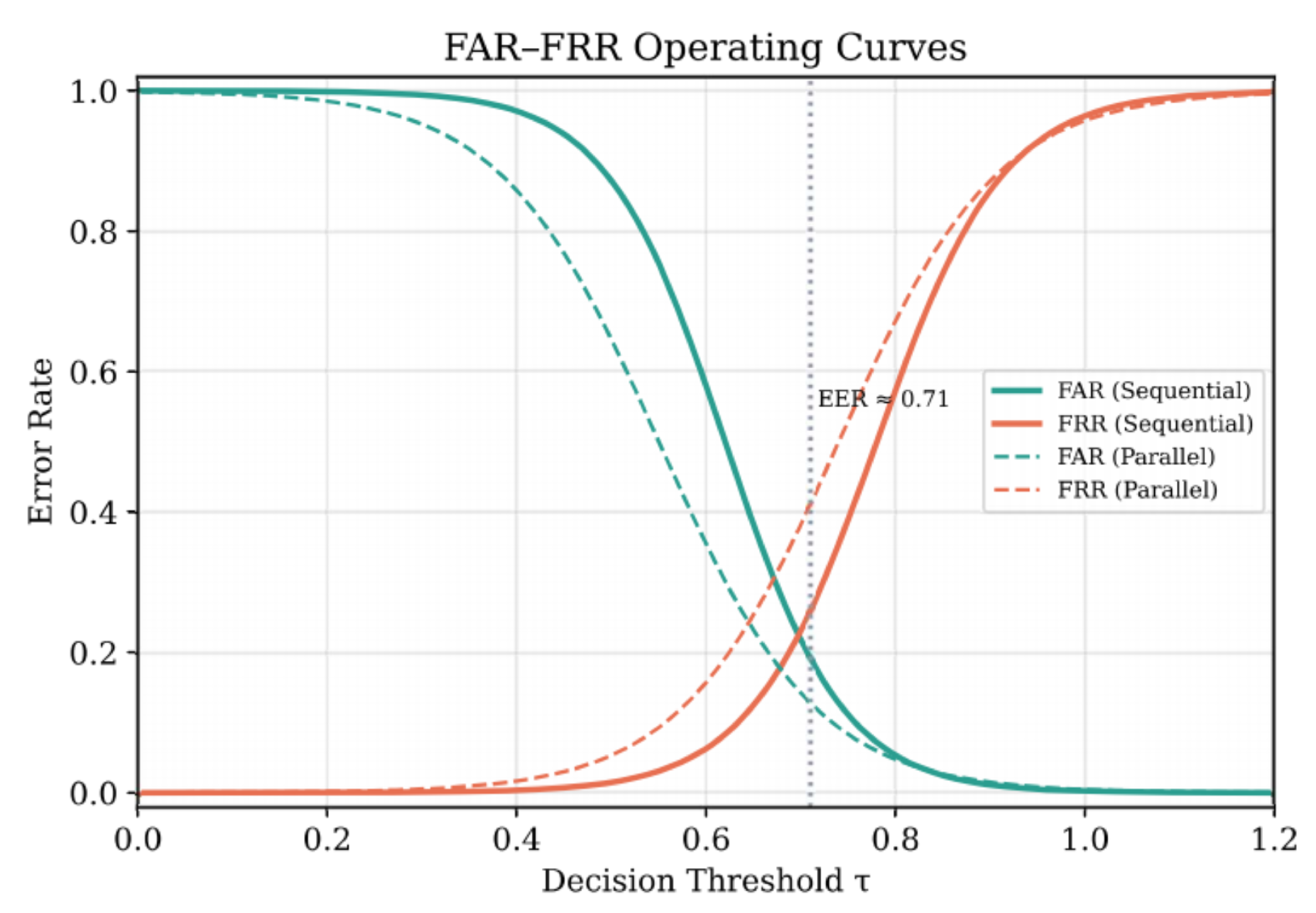
Figure 8 plots the FAR–FRR operating curves; the sequential approach exhibits a steeper transition and lower FAR at moderate-to-high thresholds, the regime relevant to high-security access control. A paired t-test across folds confirms that the FAR reduction is statistically significant ().
Figure 8.
FAR–FRR operating curves. The sequential design shows a steeper transition and lower FAR at high-security thresholds; the curves intersect (EER) near .
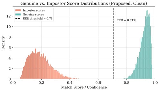
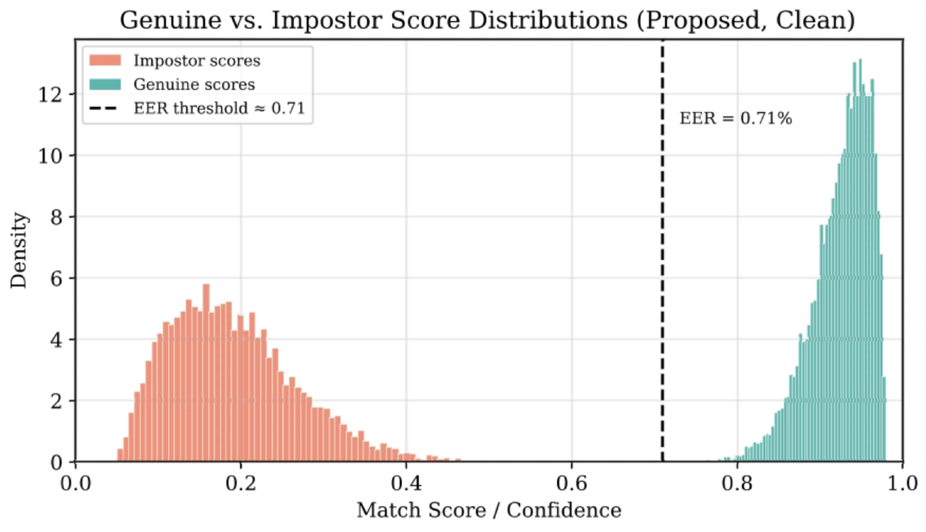
Figure 9 shows genuine and impostor score distributions. Genuine scores are concentrated approximately in the range –, whereas impostor scores are concentrated approximately in the range –.
Figure 9.
Genuine versus impostor score distributions for the proposed system. The narrow overlap at corresponds to an EER of about .
5.4. Cross-Dataset Generalization
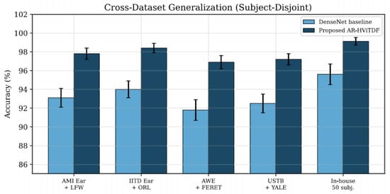
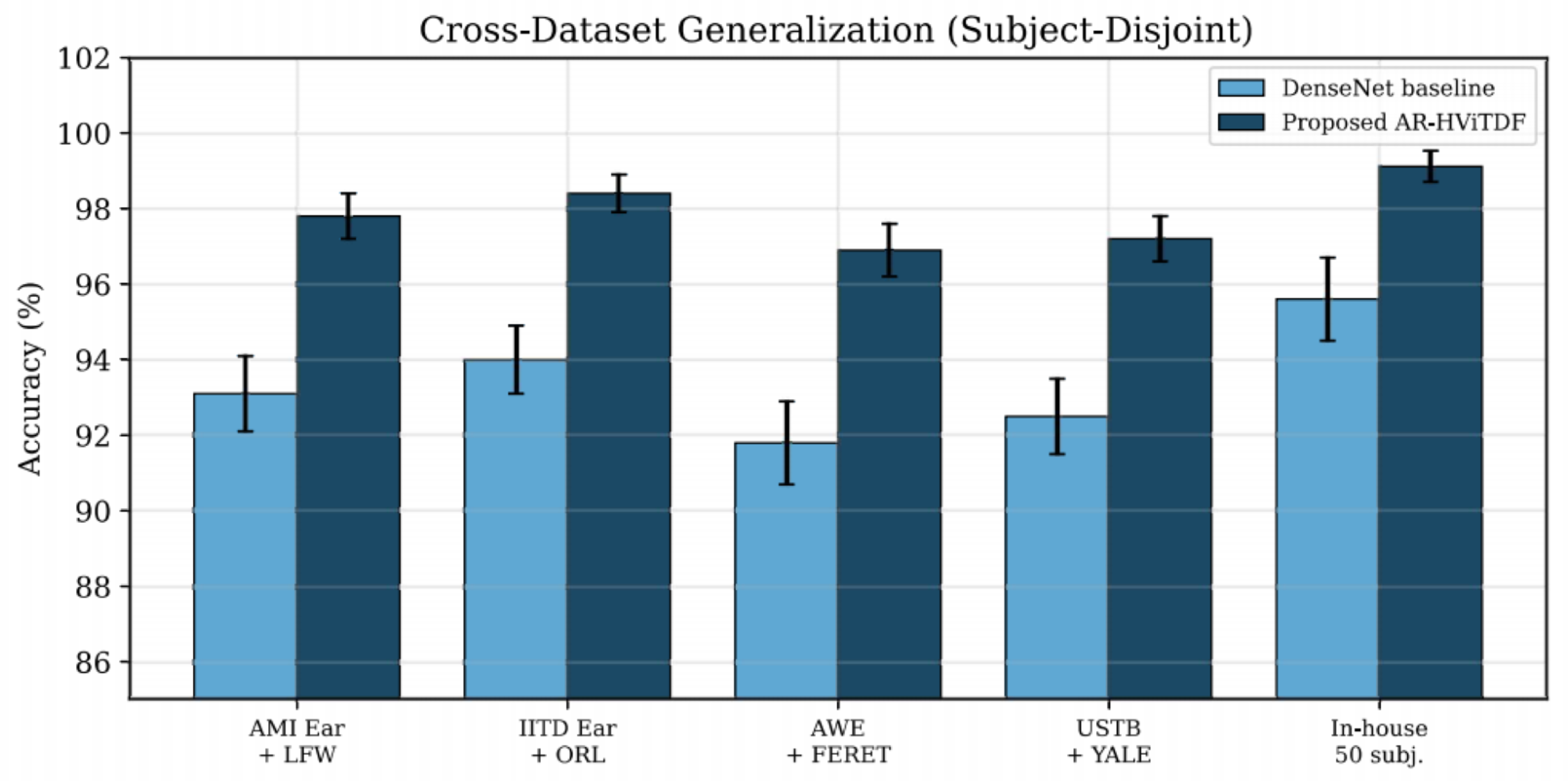
To probe demographic and sensor robustness, Figure 10 evaluates subject-disjoint performance across public ear-and-face set combinations alongside the in-house data. AR-HViTDF consistently outperforms the DenseNet baseline by approximately 4–5%.
Figure 10.
Cross-dataset generalization (subject-disjoint). The proposed model maintains high accuracy across public and in-house combinations, exceeding the DenseNet baseline throughout.
5.5. RL Convergence and Efficiency
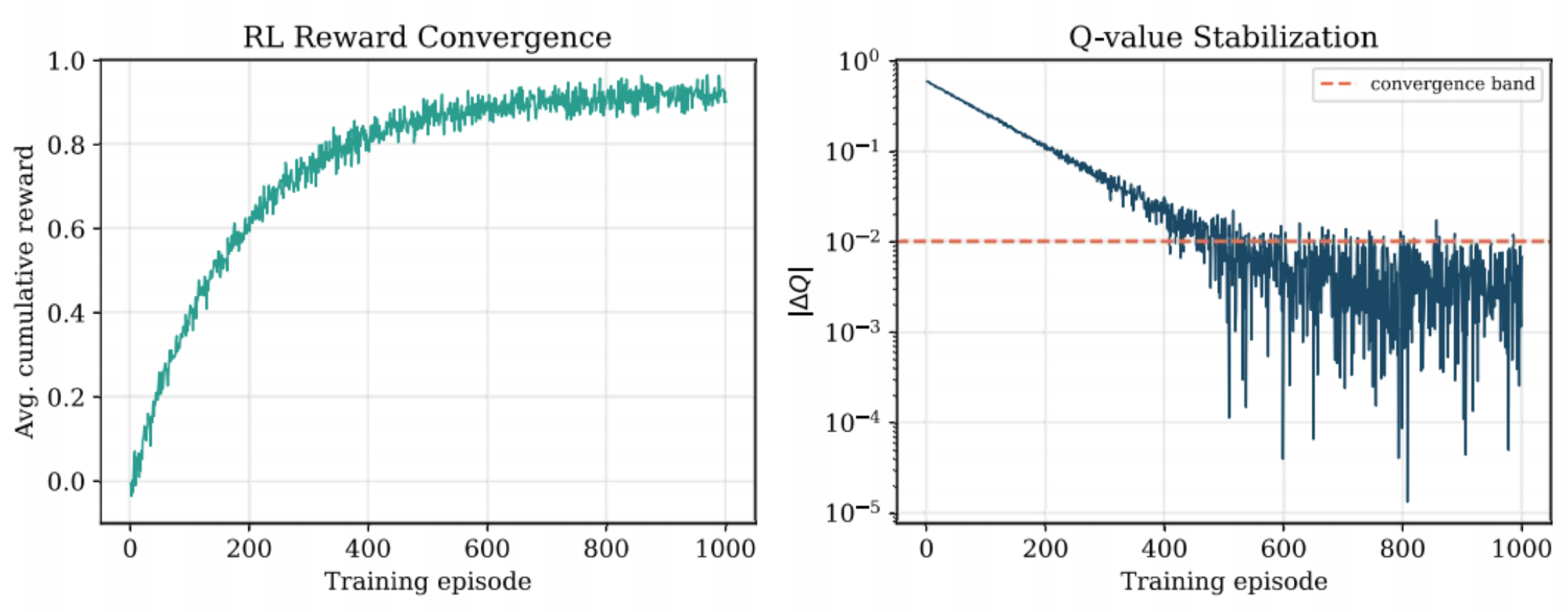
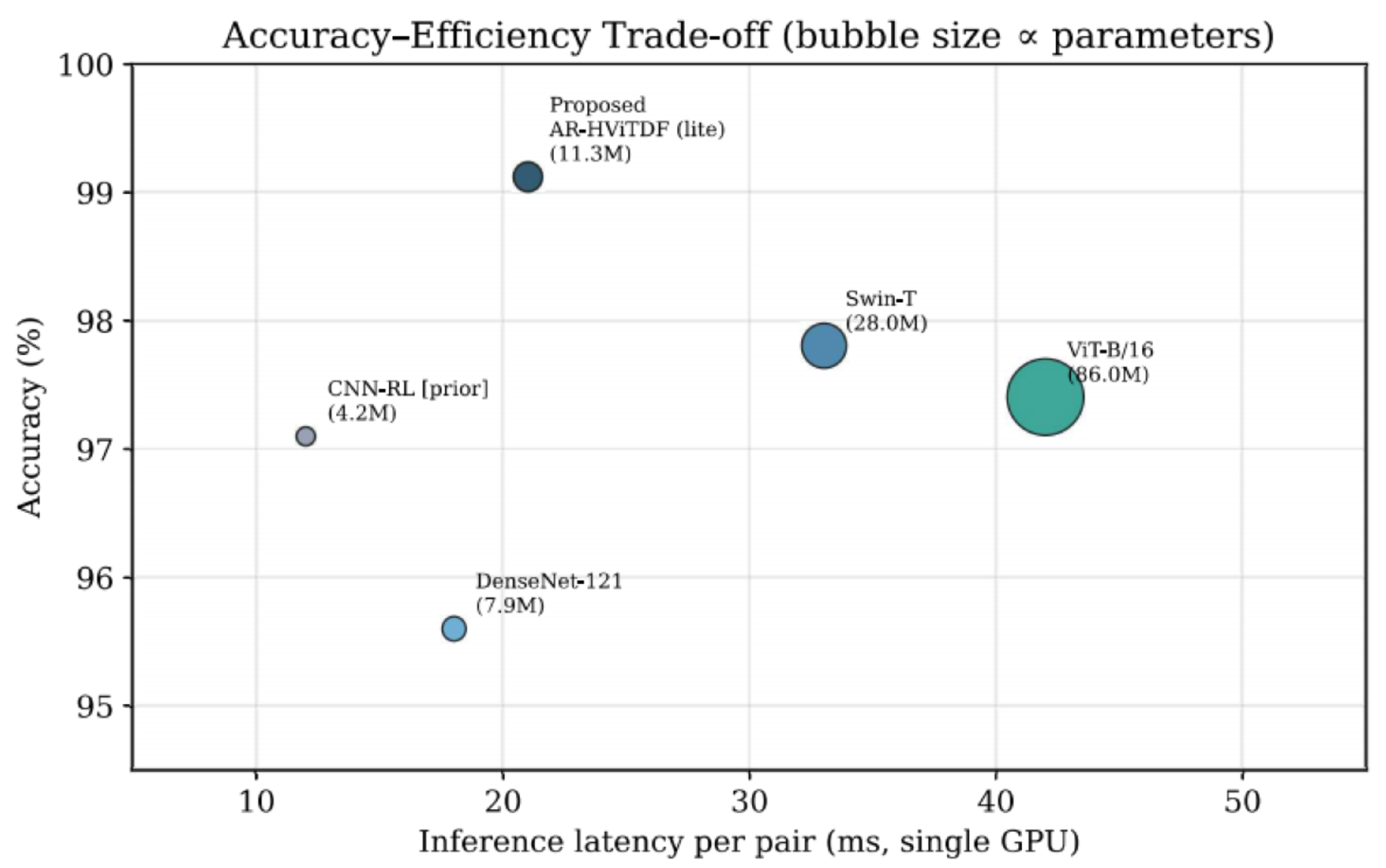
Figure 11 shows the RL agent’s average cumulative reward rising to a stable plateau and the Q-value change falling below the convergence band, confirming a learned, cost-aware threshold policy. Figure 12 situates AR-HViTDF on the accuracy-efficiency plane: at M parameters and ∼21 ms per pair on a single GPU, the lightweight design sits near the Pareto frontier.
Figure 11.
Reinforcement-learning convergence: average cumulative reward (left) and Q-value stabilization (right). The dashed band marks the convergence criterion.
Figure 12.
Accuracy–efficiency trade-off (bubble area ∝ parameters). AR-HViTDF (lite) approaches the Pareto frontier, outperforming much larger backbones at low latency.
Figure 11 shows the early episodes of high-variance and the low-reward behavior expected, while the -greedy agent explores threshold adjustments largely at random. The learned policy and the empirically estimated minimum-cost threshold closely match, which is a useful internal consistency check: the agent, given only a scalar reward, recovers the operating point that the explicit cost model, Equation (24), describes.
5.6. Ablation and Statistical Validation
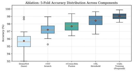
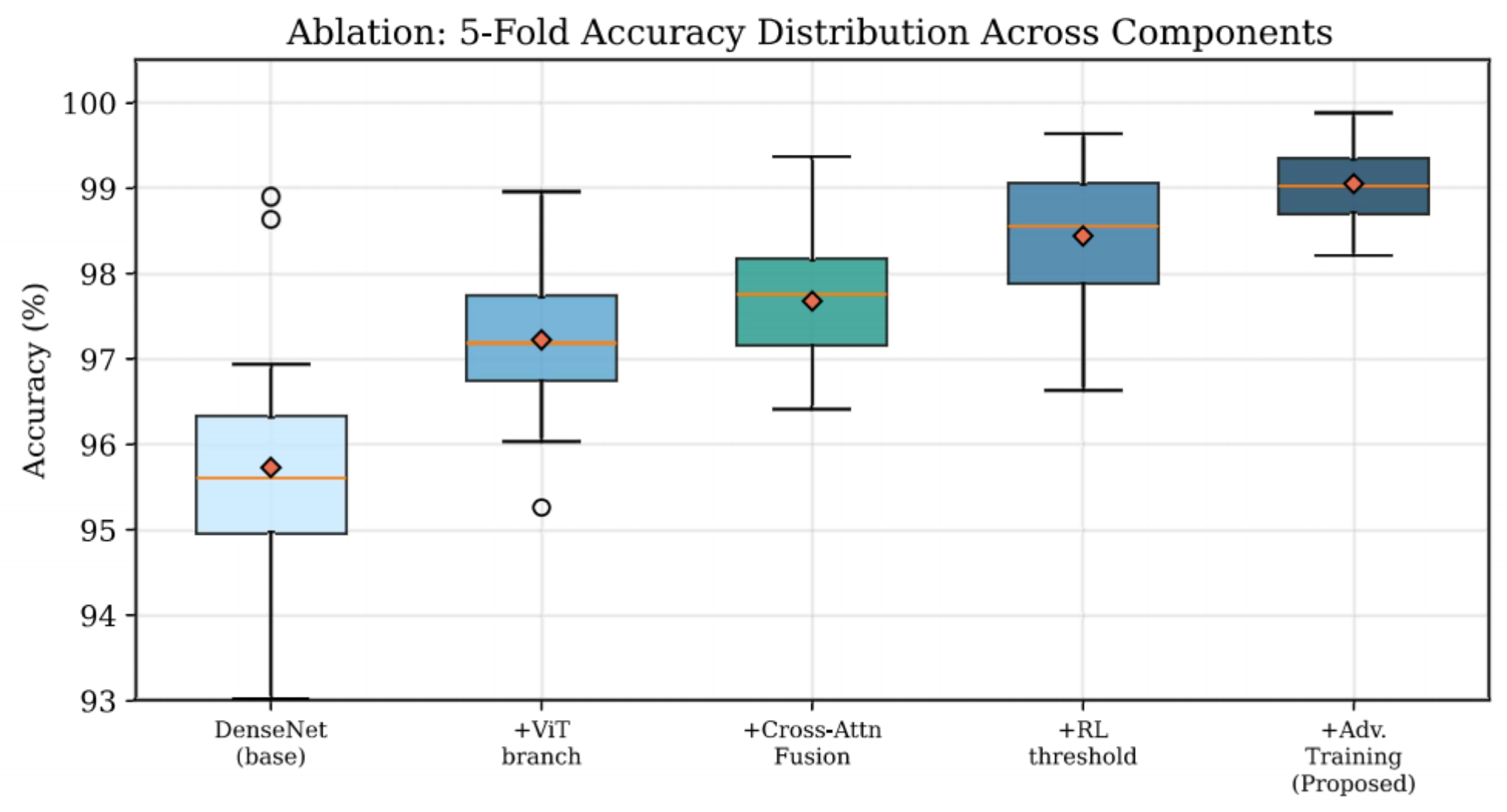
Table 5 reports a component ablation under 5-fold cross-validation with confidence intervals. Each component adds measurable value: the ViT branch and cross-attention raise clean accuracy and lower error; the RL decision layer reduces FAR/FRR; and adversarial training, while statistically unchanged (+0.12 points), is responsible for the dramatic robust-accuracy gain. Figure 13 visualizes the fold-wise accuracy distribution, showing both higher medians and tighter inter-quartile ranges as components are added.
Table 5.
Ablation results under subject-disjoint cross-validation. Robust accuracy is measured under PGD-20 at .
Figure 13.
Fold-wise accuracy distribution across the ablation configurations under subject-disjoint cross-validation. Diamonds denote the mean accuracy; median accuracy increases and variability decreases as additional components are added.
Ablation results under subject-disjoint 5-fold cross-validation. Clean accuracy is reported as mean ± standard deviation over outer folds (seeds averaged within each fold). The 95% confidence intervals are computed as , with . Robust accuracy is measured under PGD-20 at .
A one-way repeated-measures ANOVA, configured as the within-subject factor () and the subject-disjoint outer folds as experimental units (seed results averaged within each fold), detected a statistically significant difference among the five cumulative configurations—, , and partial —where the error degrees of freedom are . Because Mauchly’s test has negligible power with five folds, sphericity was not assumed; under the most conservative lower-bound correction, , the effect remains significant, , and . Post-hoc paired t-tests () with Bonferroni correction for comparisons show that the proposed model significantly exceeds Case 4 (), Case 3 () and Case 2 (). Since the configurations are nested, each adding one component to the previous one, these results indicate that the components contribute cumulatively, rather than isolating the effect of each component independently.
The single most informative row in Table 5 is the transition from Case 4 to Case 5. Clean accuracy changes only from to (95% CIs and ), whereas robust accuracy rises from to . This absence of a clean-accuracy cost at departs from the trade-off usually observed with TRADES. A plausible explanation is the small training set, on which adversarial examples may act as a regularizer and as a form of data augmentation; because this factor was not isolated, the observation should be regarded as specific to the present data. The defense is almost invisible on clean data, where a clean-only evaluation would judge it superfluous, yet it accounts for nearly all of the resilience under attack. It also corrects a misconception that recurs in the deployment literature, namely that a higher clean accuracy implies a more secure system. The DenseNet baseline of Case 1, at clean accuracy, would be ranked a strong recognizer by any clean-only benchmark, yet under PGD-20 at , its accuracy falls to , where the attack succeeds on more than three in five verification attempts. Security and clean accuracy are distinct axes, and the ablation shows that both must be reported for any system claimed to be deployable in an adversarial setting, a reporting standard that much of the prior face–ear literature has not met.
6. Study Quantification
6.1. Cross-Component Contribution
To quantify the contribution of each component beyond the ablation study, let denote the baseline accuracy of the DenseNet model, and let denote the accuracy after adding the i-th component. The normalized relative contribution is seen in Equation (22),
Using Table 6, the ViT branch contributes , cross-attention , the RL layer , and adversarial training on clean accuracy. The decisive contribution of adversarial training is on robust accuracy, where it lifts performance from to , a relative gain exceeding . The cumulative clean accuracy decomposes as Equation (23),
with each term attributable to a named component, as summarized in Table 6.
Table 6.
Component-wise cumulative contribution analysis.
6.2. Decision-Confidence Distribution
System reliability depends not only on accuracy but also on the confidence attached to each decision. Table 7 reports softmax/Q-value confidence for correct versus incorrect predictions. Correct decisions carry high, low-variance confidence (), while errors carry markedly lower confidence (). This separation enables a meaningful reject option: borderline-confidence cases can be escalated to a human operator, an important property for high-security deployment. The practical value of this separation is that it converts the system from a forced binary classifier into one that can abstain. Because the confidence of an erroneous decision is, on average, more than 12 standard deviations of the correct distribution below the correct mean, a threshold placed in the gap between the two distributions intercepts a large fraction of would-be errors at the cost of escalating only a small fraction of genuine attempts.
Table 7.
Confidence distribution for correct and incorrect predictions.
6.3. Cost-Aware Evaluation
In authentication, false acceptance is far more dangerous than false rejection. Assigning costs , the expected error cost is seen in Equation (24),
which, as a function of the threshold , becomes Equation (25),
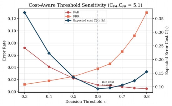
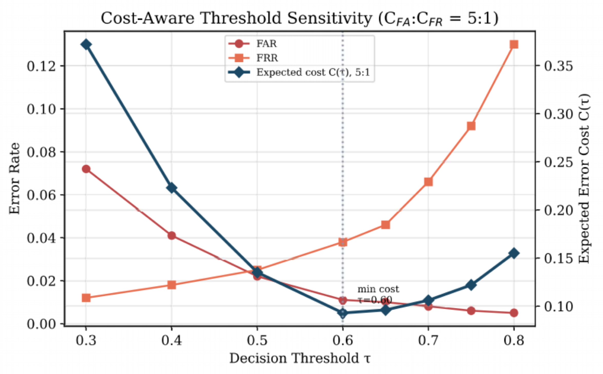
minimized by the RL agent. Table 8 and Figure 14 show that under a cost ratio, the expected cost is minimized near , where FAR is suppressed at a modest FRR expense. The RL policy converges to this region automatically, aligning the operating point with deployment priorities rather than a fixed, cost-blind threshold.
Table 8.
Threshold sensitivity under cost ratio .
Figure 14.
Cost-aware threshold sensitivity at a 5:1 false acceptance to false rejection cost ratio. Expected cost is minimized at , the region the RL learns to occupy.
The convex shape of the cost curve in Figure 14 illustrates the trade-off between the false acceptance rate (FAR) and the false rejection rate (FRR) as the decision threshold varies. At lower threshold values, the rapid reduction in FAR dominates, leading to a sharp decrease in the expected cost. The minimum cost is achieved near , beyond which further increases in the threshold provide only marginal reductions in FAR while causing a substantial increase in FRR. Consequently, the weighted cost begins to increase.
7. Conclusions and Future Scope
This paper introduces AR-HViTDF, an adversarially robust sequential multimodal biometric system that fuses face and ear characteristics through a hybrid DenseNet Vision-Transformer encoder with multi-head cross-attention, a decoupled cost-aware RL decision layer, and PGD+TRADES adversarial training. Under strict subject-disjoint cross-validation, the framework reaches clean accuracy with an EER of ; most importantly, it retains accuracy under a strong PGD-20 attack—under which a standard DenseNet collapses to —and to across six diverse attacks. Sequential authentication reduces FAR by roughly relative to parallel concatenation and widens its advantage under attack, and cross-dataset evaluation supports generalization to unseen demographics. Repeated-measures ANOVA establishes the statistical significance of each component.
7.1. Limitations and Challenges
The primary protocol relies solely on a single in-house dataset; despite the application of techniques such as augmentation, subject-disjointing, run-time averaging, and dataset validation to counter overfitting, the use of bigger and more varied datasets is necessary for increased reliability. Adversarial training raises training costs and assumes an threat model. Adaptive and unpredictable attacks pose an ever-evolving challenge. Input quality and lighting conditions are still important performance factors.
7.2. Future Directions
Future work will extend evaluation to heterogeneous, large-scale, cross-cultural datasets and sensor conditions; incorporate certified defenses (randomized smoothing) alongside empirical adversarial training; and integrate adversarially robust deployment through cancelable biometrics, homomorphic encryption, secure multi-party computation, and federated learning so that institutional collaboration improves the model without centralizing raw biometric data. Lightweight quantized variants will target on-device, IoT-class deployment, and the reject option enabled by the confidence analysis will be developed into a human-in-the-loop escalation policy for the highest-security settings.
Author Contributions
Conceptualization, S.R. and S.K.; methodology, S.R. and S.K.; software, M.A., S.R. and S.K.; validation, M.A., S.R., S.K. and A.R.W.S.; formal analysis, M.A., S.K. and S.R.; investigation, M.A., S.R., S.K. and A.R.W.S.; resources, M.A., S.R. and S.K.; data curation, S.R. and S.K.; writing—original draft preparation, M.A., S.R. and S.K.; writing—review and editing, M.A., S.R., S.K. and A.R.W.S.; visualization, M.A., S.R., S.K. and A.R.W.S.; supervision, S.R. and S.K.; project administration, M.A.; funding acquisition, M.A. and A.R.W.S. All authors have read and agreed to the published version of the manuscript.
Funding
This work was supported by the Deanship of Scientific Research, Vice Presidency for Graduate Studies and Scientific Research, King Faisal University, Saudi Arabia [Grant No. KFU266333].
Data Availability Statement
Restrictions apply to the availability of these data. Data were obtained from IIT Delhi and are available at https://www4.comp.polyu.edu.hk/~csajaykr/IITD/Database_Ear.htm (accessed on 21 September 2025) with the permission of IIT Delhi.
Conflicts of Interest
The authors declare no conflicts of interest.
References
- Tiwari, S. Biometric authentication in the face of spoofing threats: Detection and defense innovations. SSRN 2023, 9, 402–420. [Google Scholar] [CrossRef] [Scilit]
- Li, Z.; Luo, D.; Zhang, Y.; Niu, X.; Liu, H. Smart Health Monitoring: Review of Electrochemical Biosensors for Cortisol Monitoring. Adv. Healthc. Mater. 2025, 14, 2404454. [Google Scholar] [CrossRef] [Scilit]
- Bergevin, C.; Freeman, D.M.; Coffin, A. How Exceptional Is the Ear? J. Assoc. Res. Otolaryngol. 2025, 26, 203–223. [Google Scholar] [CrossRef] [Scilit]
- Sharkas, M. Ear recognition with ensemble classifiers; A deep learning approach. Multimed. Tools Appl. 2022, 81, 43919–43945. [Google Scholar] [CrossRef] [Scilit]
- Yuan, Y.; Wu, J.; Jing, Z.; Leung, H.; Pan, H. Multimodal image fusion based on hybrid cnn-transformer and non-local cross-modal attention. arXiv 2022, arXiv:2210.09847. [Google Scholar] [CrossRef] [Scilit]
- Li, X.; He, H.; Shi, J. HDCCT: Hybrid Densely Connected CNN and Transformer for Infrared and Visible Image Fusion. Electronics 2024, 13, 3470. [Google Scholar] [CrossRef] [Scilit]
- Miri Rekavandi, A.; Rashidi, S.; Boussaid, F.; Hoefs, S.; Akbas, E.; Bennamoun, M. Transformers in small object detection: A benchmark and survey of state-of-the-art. ACM Comput. Surv. 2025, 58, 1–33. [Google Scholar] [CrossRef] [Scilit]
- Sivapriya, M.S.; Suresh, S. ViT-DexiNet: A vision transformer-based edge detection operator for small object detection in SAR images. Int. J. Remote Sens. 2023, 44, 7057–7084. [Google Scholar] [CrossRef] [Scilit]
- Rastogi, S.; Kumar, S.; Ali, M.; Sait, A.R.W. Sequential Multimodal Biometric Authentication Fusion System. Mathematics 2026, 14, 1178. [Google Scholar] [CrossRef] [Scilit]
- Park, S.H.; Lee, S.-H.; Lim, M.Y.; Hong, P.M.; Lee, Y.K. A Comprehensive Risk Analysis Method for Adversarial Attacks on Biometric Authentication Systems. IEEE Access 2024, 12, 116693–116710. [Google Scholar] [CrossRef] [Scilit]
- Zhang, H.; Yu, Y.; Jiao, J.; Xing, E.; El Ghaoui, L.; Jordan, M. Theoretically principled trade-off between robustness and accuracy. In Proceedings of the International Conference on Machine Learning, Long Beach, CA, USA, 10–15 June 2019; pp. 7472–7482. Available online: https://proceedings.mlr.press/v97/zhang19p.html (accessed on 11 November 2026).
- Naseem, M.L. Trans-IFFT-FGSM: A novel fast gradient sign method for adversarial attacks. Multimed. Tools Appl. 2024, 83, 72279–72299. [Google Scholar] [CrossRef] [Scilit]
- Barbeau, L.; Lamarche-Gagnon, M.; Ilinca, F. Improving the Robustness of the Projected Gradient Descent Method for Nonlinear Constrained Optimization Problems in Topology Optimization. Int. J. Numer. Methods Eng. 2025, 126, e70068. [Google Scholar] [CrossRef] [Scilit]
- Labib, S.M.F.R.; Mondal, J.J.; Manab, M.A.; Xiao, X.; Newaz, S. Tailoring adversarial attacks on deep neural networks for targeted class manipulation using DeepFool algorithm. Sci. Rep. 2025, 15, 10790. [Google Scholar] [CrossRef] [Scilit]
- Melis, L.; Scionis, L.; Brau, F.; Pintor, M.; Biggio, B. Less is more? an ablation study on AutoAttack for adversarial robustness evaluation. In Proceedings of the 2025 International Conference on Machine Learning and Cybernetics (ICMLC), Bali, Indonesia, 13–15 July 2025; pp. 268–273. [Google Scholar] [CrossRef] [Scilit]
- Zheng, M.; Yan, X.; Zhu, Z.; Chen, H.; Wu, B. BlackboxBench: A Comprehensive Benchmark of Black-Box Adversarial Attacks. IEEE Trans. Pattern Anal. Mach. Intell. 2025, 47, 7867–7885. [Google Scholar] [CrossRef] [Scilit]
- Do, M.V.H.; Phung, D.T.; Pham, H.D.L.; Pham, Q.-D.; Hoang, V.-N.; Hoang, V.-S.; Vlaminck, M.; Luong, H.; Tran, T.-H.; Vu, H.; et al. A UAV RGB dataset and method for instance tree crown segmentation for biodiversity monitoring. Sci. Rep. 2026, 16, 5788. [Google Scholar] [CrossRef] [Scilit]
- Huang, Q. Multimodal Biometrics Fusion Algorithm Using Deep Reinforcement Learning. Math. Probl. Eng. 2022, 2022, 8544591. [Google Scholar] [CrossRef] [Scilit]
- Abidi, S.M.H.; Hassan, S.A.; Raza, S.M.; Beliatis, M.J. Advances in Face Recognition: A Comprehensive Review of Feature Extraction and Dataset Evaluation. Electronics 2026, 15, 338. [Google Scholar] [CrossRef] [Scilit]
- Yadav, A.K.; Pateriya, R.K.; Gupta, N.K.; Gupta, P.; Saini, D.K.; Alahmadi, M. Hybrid machine learning model for face recognition using SVM. Comput. Mater. Contin. 2022, 72, 2697–2712. [Google Scholar] [CrossRef] [Scilit]
- Pahuja, S.; Goel, N. Multimodal biometric authentication: A review. AI Commun. Eur. J. Artif. Intell. 2024, 37, 525–547. [Google Scholar] [CrossRef] [Scilit]
- Mehta, R.; Shukla, S.; Pradhan, J.; Singh, K.K.; Kumar, A. A vision transformer-based automated human identification using ear biometrics. J. Inf. Secur. Appl. 2023, 78, 103599. [Google Scholar] [CrossRef] [Scilit]
- Kaplesh, P.; Gupta, A.; Bansal, D.; Sofat, S.; Mittal, A. Vision transformer for contactless fingerprint classification. Multimed. Tools Appl. 2025, 84, 31239–31259. [Google Scholar] [CrossRef] [Scilit]
- Safwat, S.; Mahmoud, A.; Eldesouky Fattoh, I.; Ali, F. Hybrid Deep Learning Model Based on GAN and RESNET for Detecting Fake Faces. IEEE Access 2024, 12, 86391–86402. [Google Scholar] [CrossRef] [Scilit]
- Panda, S.P. Adversarial Machine Learning: Analyzing Carlini & Wagner Attacks. In Proceedings of the 2025 4th International Conference on Innovative Mechanisms for Industry Applications (ICIMIA), Tirupur, India, 3–5 September 2025; pp. 1231–1236. [Google Scholar] [CrossRef] [Scilit]
- Rastogi, S.; Duttagupta, S.P.; Guha, A.; Prakash, S. Palm vein pattern: Extraction and Authentication. In Proceedings of the 2020 IEEE International Conference on Machine Learning and Applied Network Technologies (ICMLANT), Hyderabad, India, 20–21 December 2020; pp. 1–5. [Google Scholar] [CrossRef] [Scilit]
- Alharbi, A.; Alsubaie, N.; Alharbi, H.; Aldayel, M. Deep Learning-Based Fingerprint-Vein Biometric Fusion: A Systematic Review with Empirical Evaluation. Appl. Sci. 2025, 15, 8502. [Google Scholar] [CrossRef] [Scilit]
- Alay, N.; Al-Baity, H.H. Deep Learning Approach for Multimodal Biometric Authentication System Based on Fusion of Iris, Face, and Finger Vein Traits. Sensors 2020, 20, 5523. [Google Scholar] [CrossRef] [Scilit]
- Kim, H.; Papamakarios, G.; Mnih, A. The lipschitz constant of self-attention. In Proceedings of the International Conference on Machine Learning, Online, 18–24 July 2021; pp. 5562–5571. Available online: https://proceedings.mlr.press/v139/kim21i (accessed on 10 August 2026).
- Watkins, C.J.; Dayan, P. Q-learning. Mach. Learn. 1992, 8, 279–292. [Google Scholar] [CrossRef] [Scilit]
- Jaakkola, T.; Jordan, M.; Singh, S. Convergence of stochastic iterative dynamic programming algorithms. In Advances in Neural Information Processing Systems 6; Morgan Kaufmann: San Mateo, CA, USA, 1993; pp. 703–710. [Google Scholar]
- Tsitsiklis, J.N. Asynchronous stochastic approximation and Q-learning. Mach. Learn 1994, 16, 185–202. [Google Scholar] [CrossRef] [Scilit]
- Even-Dar, E.; Mansour, Y. Learning rates for Q-learning. J. Mach. Learn. Res. 2003, 5, 1–25. [Google Scholar]
- Tsitsiklis, J.N.; Van Roy, B. Feature-Based Methods for Large Scale Dynamic Programming. Mach. Learn. 1996, 22, 59–94. [Google Scholar] [CrossRef] [Scilit]
- Singh, S.; Jaakkola, T.; Jordan, M. Reinforcement learning with soft state aggregation. In Advances in Neural Information Processing Systems; MIT Press: Cambridge, MA, USA, 1994; pp. 361–368. [Google Scholar]
- Gordon, G.J. Reinforcement learning with function approximation converges to a region. In Advances in Neural Information Processing Systems 13; MIT Press: Cambridge, MA, USA, 2000; pp. 1040–1046. [Google Scholar]

Disclaimer/Publisher’s Note: The statements, opinions and data contained in all publications are solely those of the individual author(s) and contributor(s) and not of MDPI and/or the editor(s). MDPI and/or the editor(s) disclaim responsibility for any injury to people or property resulting from any ideas, methods, instructions or products referred to in the content. |
© 2026 by the authors. Licensee MDPI, Basel, Switzerland. This article is an open access article distributed under the terms and conditions of the Creative Commons Attribution (CC BY) license.