


Abstract
Concurrent defects in rotating components produce overlapping vibration components, complicating the recognition of defect combinations absent from training. We formulate this task as compositional multi-label learning and propose a compositional evidence-grounded framework (CEG-LLM). The model uses a frozen large language model as a sequence encoder, with trainable low-rank adapters and four sigmoid defect outputs. Continuous waveform tokens and nominal characteristic-order descriptors represent the signal, while a four-node composition graph conditions label-wise attention. Spectral alignment and compositional regularization guide training, and a fixed template links predictions to structured signal records. On one dataset collected from a rotating component at 1500 rpm, CEG-LLM achieves an observed-state macro-F1 of 0.941. Corresponding values are 0.922 for a one-dimensional vision Transformer (ViT), 0.912 for a signal-to-text language encoder, and 0.900 for a convolutional neural network (CNN). Mean exact match across six withheld defect pairs is 0.767, and macro-F1 at dB is 0.819. A top-token versus random-mask deletion contrast of 0.207 indicates sensitivity to the selected representation under that intervention. These results assess recognition of unseen defect combinations and representation sensitivity within the evaluated operating condition.
Keywords:
large language model; multi-label learning; applied mathematics; compound defect detection; rotating components MSC:
68T07; 68T10; 62H30
1. Introduction
Compound defect detection is a multi-label inference problem in which overlapping signal components must be associated with their underlying defect types. Rotating components provide a representative application of this problem in mechanical equipment. A local defect changes contact forces, excites structural resonances, and may accelerate damage elsewhere. The resulting signal contains multiple impact trains, modulation products, transfer-path effects, and operating noise [1]. Its spectrum is more complex than a simple union of isolated defect patterns. Strong responses can mask weaker components, while shared harmonics can blur the distinction between defect sources [2,3,4]. A reliable detector must distinguish a second defect from harmonics generated by the first. Recent work combines physics-informed adaptation, nonstationary signal models, and operating-condition-aware measurements [5,6,7,8]. Such methods extend detection beyond closed-set recognition from a single representation [9]. Edge–cloud monitoring supports continuous data collection, but additional observations alone do not resolve the attribution of signal components to defects [10,11].
Many learning-based detectors map each signal window directly to a class identifier [12]. This formulation is suitable when every class appears in training [13], but becomes restrictive when each defect combination requires a separate class. The number of possible combinations grows rapidly, and some pairs may be absent from training [14]. A class identifier also provides no indication of which signal components support each detected defect. Multi-label and zero-shot methods reduce this combinatorial burden by modeling defect attributes or semantic prototypes [15,16,17,18]. Recent zero-shot detectors represent unseen compound states through semantic embedding, adaptive attribute weighting, or class-aware latent generation [19,20,21]. Label-vector generation and hybrid semantic attributes offer related strategies without requiring samples from every combination [22,23]. A model may nevertheless associate an attribute with a spurious resonance rather than a repeatable defect order [24]. Evaluation should therefore examine both the predicted label combination and the physical evidence associated with its components.
Large language models (LLMs) provide pretrained sequence representations that can be adapted to numerical signals [25]. Vibration-language models combine multiple vibration views with language representations [26]; explainable machinery models and FD-LLM align engineering information with language-compatible features [27,28]. Discretized-signal and human-in-the-loop approaches offer other input and interaction designs [29,30]. These studies support the feasibility of adapting language representations to vibration signals, although they do not establish that a language backbone is necessary. In this work, the backbone encodes continuous signal embeddings and contextual tokens. The problem is to represent known atomic defects in a withheld pair while retaining a separate, inspectable evidence record for each predicted label.
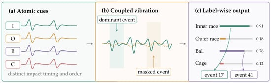
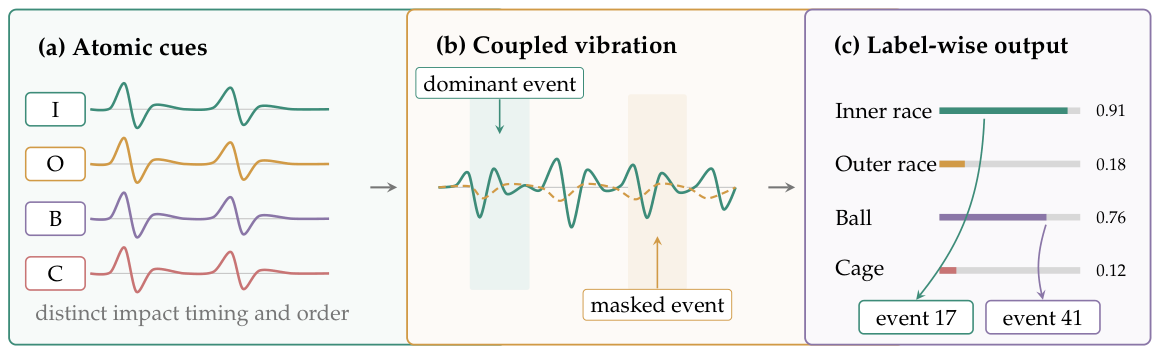
CEG-LLM combines local waveform tokens, nominal physical-order information, and four atomic defect queries to estimate a four-bit label vector. This representation permits known defect types to be recombined without assigning a distinct class to every combination. Beyond semantic prototype transfer or unseen-class feature synthesis, the framework retains token origins and evaluates label-conditioned representation sensitivity. Whereas some language models generate diagnostic text [31], CEG-LLM reports labels, scores, and origin records through a fixed template. The composition graph and evidence objective are evaluated separately to distinguish their contributions from the overall encoder contribution. Figure 1 illustrates the relationship between overlapping vibration components and separate label outputs.
Figure 1.
Illustration of compound defect detection with separate label outputs.
The study addresses the need to evaluate compositional recognition, alignment with available physical cues, and prediction sensitivity as distinct properties. Its contributions are summarized as follows:
- A signal representation that preserves local waveform information and explicitly records the availability of nominal characteristic-order evidence, including the cage-resolution limit.
- A four-label decoder conditioned by a composition graph, which represents combinations of known defect types without introducing a separate class for each pair.
- An evaluation that distinguishes label detection, withheld-pair exact match, and representation-deletion contrast, with attention and spectral overlap used to assess the associated evidence.
2. Related Work and Problem Formulation
2.1. Compound Defect Detection
Signal-based methods retain physically inspectable components before classification [32]. Resonance-demodulation semantics focus on informative resonances [33], while learnable wavelets adapt the representation to variable speed [34]. These mechanisms help preserve defect signatures, but overlapping sources still require separate label decisions. Multi-label domain adaptation directly models concurrent labels [2,35]; its transfer objective differs from withholding a compound pair within one dataset [36]. Physically structured features concern how signals are represented, whereas compositional recognition concerns how known defect types are combined in the output space. Table 1 Representation choices relevant to compound defect diagnosis in rotating components.
Table 1.
Representation choices relevant to compound defect diagnosis in rotating components.
2.2. Language Encoders for Vibration Signals
FD-MVLLM aligns multiple vibration views with a language backbone [26]. Explainable machinery LLMs and FD-LLM use language-compatible engineering representations [27,28]; discretized-signal diagnosis changes the input encoding [29]. These approaches motivate cross-modal adaptation, but their input and explanation mechanisms are not interchangeable. CEG-LLM preserves continuous patches and uses a fixed multi-label output head. Its template report is evaluated as structured attribution because the encoder is not used to generate diagnostic text. Isolating the effect of language pretraining would require comparisons with a matched non-language Transformer and a matched randomly initialized backbone.
2.3. Event-Driven Detection
The continuous time-frequency-gradient WPPM-SNN introduced the experimental dataset used in this study [37]. Its event-driven processing provides an alternative computational approach to a large frozen encoder. Sparse processing alone, however, does not establish which physical evidence supports each label. A matched comparison with the dataset-source method would help assess the role of event representations relative to encoder performance.
2.4. Semantic Composition and Transfer
Fault-semantics learning constructs a relationship between single and compound fault descriptions [38,39]. Generative semantic alignment instead connects fault semantics with synthesized feature representations [40]. Adaptively weighted semantic autoencoding emphasizes attribute weighting [20], while class-aware variational generation learns semantic representations through a generative latent model [21]. These mechanisms reduce the need for examples of every target combination [41,42], but they do not by themselves validate the origin of each label’s evidence. CEG-LLM differs in preserving token-origin records and auditing separate label queries. Its withheld-pair setting retains all four atomic defect types during training, so it addresses unseen combinations rather than novel defect types or cross-machine transfer.
2.5. Task Definition
Let denote a vibration segment, and let contain the available rotational speed, sampling frequency, and equipment geometry. Load can be included as an additional covariate when it is recorded. The four-component defect label vector is
The four labels denote inner-race, outer-race, ball, and cage defects. Normal operation is represented by the all-zero vector, so no separate normal label is predicted. Application to another machine requires a corresponding atomic defect vocabulary and physical-order library. Each compound sample in the present dataset activates two defect locations. The detector estimates
where is a defect composition graph. This factorization assumes conditional independence of the outputs given the shared input representation and graph. Classifier chains instead factorize the joint distribution as , explicitly conditioning later decisions on earlier labels [43]. Chains introduce label-order dependence and possible error propagation, while the four parallel queries avoid sequential decoding but may leave residual output dependence unmodeled. The present evaluation does not include a comparison with classifier chains. For each label, denotes an attention distribution over signal-origin hidden states, subject to the attribution limits described below.
3. Proposed CEG-LLM
3.1. Architecture Overview
The architecture in Figure 2 comprises an event tokenizer, a graph prompt encoder, low-rank adapters, and a label-wise decoder. The backbone weights remain fixed, while the adapter weights and task modules are optimized for defect detection. Freezing the backbone reduces the number of trainable parameters but retains the costs of forward computation and activation storage.
Figure 2.
CEG-LLM architecture.
For each sample, the tokenizer produces continuous patch tokens and sparse evidence tokens . The graph prompt encoder combines with operating metadata and the defect graph. The resulting prompt is concatenated with reprogrammed patch embeddings and passed through the frozen LLM. The detector queries hidden states with one prototype per atomic defect and returns both detection probabilities and evidence weights.
3.2. Physics-Anchored Event Tokenizer
A high-rate waveform must be mapped to a suitable representation before entering a language-model encoder. Encoding each amplitude as text produces long sequences that depend on amplitude quantization. Global statistics compress the signal but discard the local structure of impacts. CEG-LLM retains continuous local patches together with sparse physical-order anchors.
The normalized signal is divided into J overlapping patches . For each patch, the tokenizer computes a compact descriptor
Here indexes the I/O/B/C anchor channels, with a validity mask indicating unavailable anchors. The quantities , , and denote root-mean-square amplitude, kurtosis, and crest factor, respectively; denotes the quality indicator. Patches have length and are extracted with stride S. The resulting patch count is , and the overlap fraction is .
Spectral descriptors are computed from an analysis context that contains patch j. This context is defined as , with start index , length , and duration . Separating the patch and context is necessary because a 128-point patch cannot resolve low characteristic orders at the sampling rate considered here. Let denote the context envelope spectrum, and let indicate whether the context duration resolves the order of defect c. The corresponding normalized band energy is
Rotational speed and component geometry determine the center frequency . The associated band set is . Here, and contain the harmonic and shaft-sideband indices, respectively, and is the band half-width. This construction accounts for the characteristic order, its harmonics and sidebands, and the specified frequency tolerance. Because these sets can overlap, shared frequency bins cannot uniquely identify a defect. For context duration , the validity rule requires at least two nominal cycles. Masking an unavailable band distinguishes insufficient frequency resolution from a measured absence of energy.
For the rotating component used in the experimental evaluation, let denote shaft rotation frequency and n the number of rolling elements. Let d, D, and denote rolling-element diameter, pitch diameter, and contact angle, respectively. The nominal characteristic frequencies are
At a shaft speed of 1500 rpm, the rotation frequency is Hz. The nominal geometry , mm, mm, and gives , , , and Hz. These calculated frequencies describe nominal kinematic orders rather than measured spectral peaks. The component catalogue lists eight balls with a diameter of 4.762 mm [44]. The 5 mm diameter used in this order calculation is a rounded nominal value. Ball defects can also excite twice the ball-spin frequency (BSF), nominally 93.75 Hz for the stated geometry. A peak at BSF or twice BSF provides a candidate physical cue, but is insufficient on its own to identify a ball defect.
Each window spans s, giving 12 Hz Fourier-bin spacing; a 128-point patch alone gives 384 Hz. Two nominal ball-spin cycles require at least samples, with approximately 23.4 Hz bin spacing. Zero-padding does not improve physical resolution. Inner-race shaft sidebands occur at 100 and 150 Hz, and 150 Hz also equals twice the nominal outer-race frequency. Shared bins therefore require interpretation together with the waveform and context features. The nominal cage fundamental completes only 0.781 cycles in a full window, so its order anchor is masked.
Resonance bands are selected using the training partition before test-set assessment. This step supports envelope extraction for order-based description; the present comparison does not isolate the contribution of a particular band-search algorithm. For each candidate band, a fixed bandpass filter and Hilbert transform produce an envelope. The envelope spectrum is then expressed in order coordinates . All candidate frequencies and tolerances are fixed before the test set is inspected. Each local descriptor includes a quality flag for clipping, nonstationary speed, or a weak envelope. The decoder receives this flag, allowing difficult windows to remain in the analysis. If rotational speed is unavailable at inference, requires an independent estimate together with its uncertainty. This extension is outside the evaluation provided by the fixed-speed dataset.
The continuous token combines the patch, descriptor, and positional embedding:
Sparse event tokens are created only when a score exceeds a threshold selected from the training and validation partitions:
The indicator performs hard event selection and has zero gradient almost everywhere. Consequently, the threshold operation does not provide an ordinary differentiable path. The continuous patch stream preserves waveform information, while the discrete event stream selects explicit event records. Continuous tokens remain available even when their event scores fall below the threshold. Ambiguous signal information is therefore retained despite the binary event-selection decision.
Each event token carries an origin tuple identifying its patch, filtering band, nominal order, and quality flag. This metadata locates the token’s construction interval, but self-attention subsequently combines information across tokens. The final hidden state is therefore not restricted to information from that interval. Continuous patches also retain waveform responses outside the nominal order anchors. A cage label can consequently be predicted from waveform and shared context features even when its order anchor is masked. Such a prediction lacks resolved cage-frequency support and is excluded from the I/O/B order-overlap assessment.
3.3. Defect Composition Graph and Evidence Prompt
The label graph contains one node for each atomic defect in the equipment under study. Edges encode mechanically compatible co-occurrence without treating observed combinations as separate classes. The graph is specified by the task definition, independently of test labels. Node features combine a learned label prototype, equipment-specific order descriptors, and a short definition of the defect location.
A two-layer graph attention operator updates the label prototypes:
Here, denotes the aggregation neighborhood for query c. When included, a self-message carries the node’s own representation without imposing an additional co-occurrence constraint. Because all six pairs are admissible, the binary topology is the complete graph . The graph supports message exchange among the four atomic defect queries. Query differences arise from node features, learned attention, and edge attributes; the topology itself excludes no defect pair.
The prompt supplies operating context and signal descriptors. The following text illustrates its semantic structure:
- Sampling rate: 49,152 Hz.
- Shaft speed: 1500 rpm.
- Nominal orders: I 5.000, O 3.000, B 1.875, C 0.375.
- Cage anchor: unavailable.
- Event records: patch index, band, order energy, score, quality.
- Output: four atomic-label probabilities.
The orders in this context follow the stated nominal geometry. Decimal strings describe the operating context, while waveform patches enter as continuous embeddings. Event records attach patch identity, order energy, and quality to the corresponding signal representation.
3.4. Cross-Modal Reprogramming and Parameter-Efficient Adaptation
Signal tokens are mapped into the embedding space of the frozen LLM. Let denote a learned bank of M prototypes initialized from that space. Each patch token is represented by an attention-weighted combination of these prototypes:
The LLM processes the sequence , which concatenates prompt and signal embeddings. Low-rank adaptation (LoRA) is applied to the query and value projections:
where the backbone matrix is frozen, r is the adapter rank, and and are trainable. The symbol denotes the reprogramming projection and is distinct from the decoder-query projection . The pretrained backbone transforms the input sequence even though its original weights are fixed; adaptation changes the low-rank projections and task representations.
Training updates the signal projection, graph encoder, low-rank matrices, and decoder while holding backbone weights fixed. For adapted layers with two square query/value projections of width D, the adapter contribution is approximately parameters, excluding the task modules.
3.5. Evidence-Constrained Multi-Label Decoder
The decoder assigns one query to each atomic defect type. Cross-attention is normalized over hidden states corresponding to signal-origin tokens, with prompt-only states excluded from both evidence normalization and deletion. For label c, attention over these hidden states is given by
The attention vector ranks signal-origin hidden states separately for each label. After multi-layer self-attention, incorporates information from other signal and prompt positions. Excluding prompt-only states from normalization therefore does not remove their contextual influence on . Mapping attention weights to token origins visualizes the decoder readout at those positions, subject to this contextual dependence [45].
Prediction accuracy alone does not establish whether the associated evidence is faithful. Let denote patch impulsiveness normalized using training data. The physics score is computed from the input and kept independent of classifier updates. When , normalization gives the target distribution
The context length determines how this regularizer varies across patches. If is the same full window for every j, then . For each valid nonzero anchor, the target reduces to , with identical shapes for I, O, and B. A shorter sliding context can produce distinct local shapes, but reduces frequency resolution and may increase band overlap. Thus, defines a physical-band alignment target without guaranteeing label-specific physical localization.
For positive labels with a valid order anchor, the decoder is encouraged to align with this distribution. The target remains fixed for each input and cannot drift with the learned event gate. Labels without a resolvable anchor are excluded from the spectral alignment term. The exclusion applies to cage labels in an isolated 4096-point window. A characteristic order is not assumed to be sufficient for classification. The intervention assesses sensitivity of the learned representation to selected tokens.
Let be the signal-origin token pool, excluding prompt-only positions, and the K highest-ranked members for positive label c. For a specified masking operator , the top-token probability drop is
For a size-matched random set , define the reported deletion contrast as
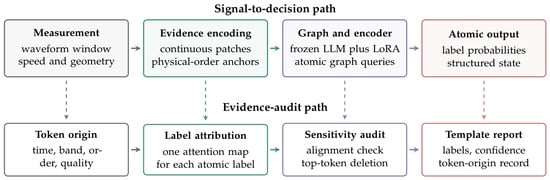
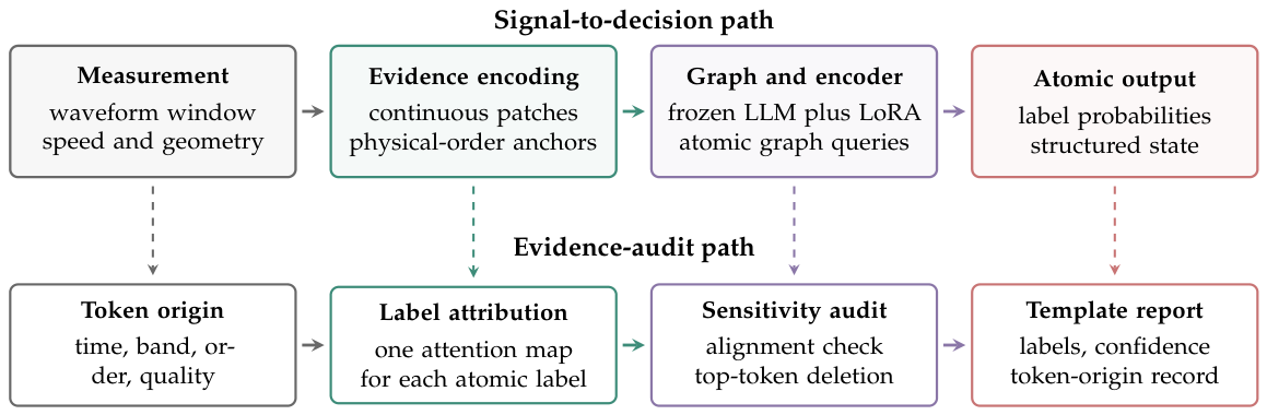
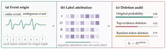
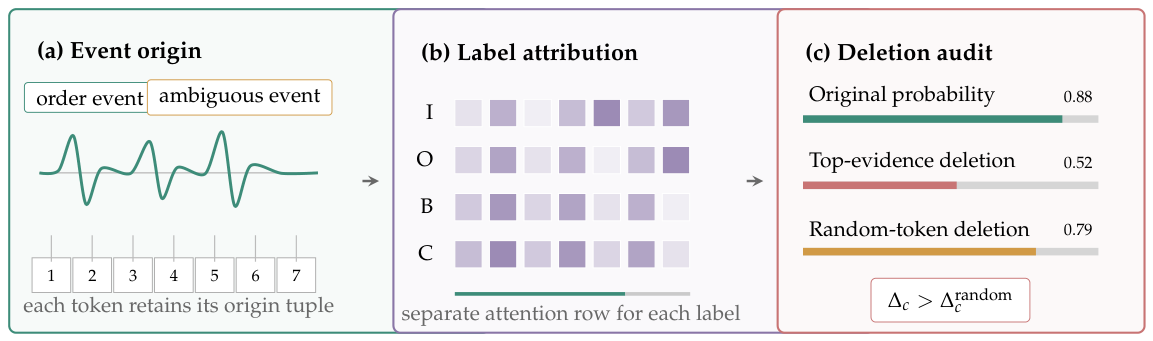
The deletion contrast in Equation (16) compares the probability drops from the two interventions. Both token sets are drawn from the same signal-origin pool and have cardinality K. Matching cardinality controls the number of affected tokens, while the intervention remains defined at the representation level. Masking can shift the input distribution, and zero replacement, mean replacement, and token removal induce different perturbations. The contrast therefore measures prediction sensitivity under the specified intervention. It is distinct from a remove-and-retrain assessment such as ROAR [46]. Figure 3 illustrates the evidence-grounding process, including token-origin tracking, label-conditioned attention, and representation deletion for assessing prediction sensitivity.
Figure 3.
Workflow illustration of origin tracking, label-conditioned attention, and representation deletion.
Order overlap describes alignment between the label readout and valid physical-order support. An attention-mass expression of this alignment is , where for an available anchor assigned to and zero otherwise.
3.6. Training Objective and Inference
The classification term uses class-balanced binary cross entropy over the four atomic defects:
Define . The evidence loss is zero when this set is empty and otherwise equals
For an observed two-defect training sample, compositional regularization encourages alignment between its representation and the sum of the two active label prototypes:
Here, is the mean hidden representation of the signal tokens, and is the graph-conditioned prototype of defect c. The term is zero for normal and single-defect samples. It is also omitted when either cosine argument has zero norm. The complete objective is
Here, denotes the complete set of trainable model parameters. All nonnegative loss coefficients and the positive and negative class weights are selected or estimated using training and validation data only. Normal operation corresponds to four negative defect labels, which rules out simultaneous normal and defect outputs by construction. No sample of a withheld pair contributes to the compositional loss. Its atomic prototypes are trained through the corresponding single-defect states and the other observed pairs. This exclusion ensures that the evaluation concerns a combination absent from training.
Per-label decision thresholds are selected using the validation set. Temperature scaling is fitted on a held-out portion of the training set, and calibration is evaluated using expected calibration error (ECE). A fixed reporting template associates predicted labels with their highest-ranked evidence tokens, including patch time, resolvable spectral order, and confidence. This template does not generate additional causal explanations beyond the recorded evidence. If no defect probability exceeds its threshold, a separate quality check determines the operational output. Windows that pass this check are reported as normal; other windows are reported as “insufficient evidence.” Primary detection metrics are computed from the four thresholded defect probabilities before the quality check.
4. Experimental Evaluation
4.1. Evaluation Setting
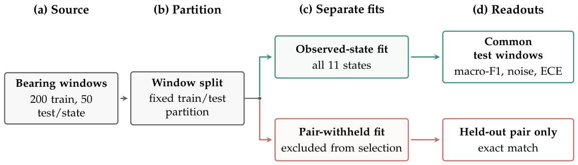
Experiments used the NSK 6200 bearing dataset introduced for continuous time-frequency-gradient compound defect detection [37]. It contains normal operation, four single-defect states, and all six pairs of inner-race, outer-race, ball, and cage defects. Each state provides 200 training windows and 50 test windows. Every window contains 4096 samples acquired at 49,152 Hz and a shaft speed of 1500 rpm.
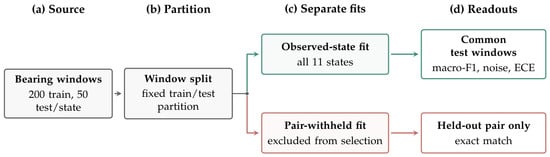
Observed-state detection uses all 11 states and is evaluated separately from the six leave-one-pair-out settings. In each leave-one-pair-out setting, the target pair is excluded from optimization, validation, and fitted preprocessing. Its atomic defect types remain represented through single-defect states and the other pairs. This protocol tests generalization to unseen combinations of known defect types within the same dataset. It does not evaluate new atomic defect types or transfer to another machine. The result records contain five seed values for each of six pair-index entries. For the observed-state summary, the six entries are averaged within each seed and are not treated as independent observed-state folds. Figure 4 illustrates the experimental evaluation settings, including data partitioning, observed-state detection, and withheld-pair evaluation with their corresponding performance metrics.
Figure 4.
Window-based evaluation settings.
The CNN applies local filtering to the normalized waveform, while the ViT applies self-attention to one-dimensional patches. The signal-to-text language encoder receives signal statistics and spectral summaries as textual input. CEG-LLM combines physical descriptors, graph conditioning, and an evidence objective. The comparison covers convolutional, patch-attention, textual-signal, and structured-evidence representations. Because these methods differ in several components, their results evaluate the complete implementations without isolating the effect of language pretraining.
The ablation study removes physical anchors, the graph-conditioned module, or the evidence loss individually. The “global statistics” variant replaces local patch and event inputs with a window summary. The “compact encoder” variant replaces the language backbone with a smaller encoder while retaining the other proposed task modules. Thus, three variants remove individual components, and two substitute the input representation or encoder. The compact-encoder comparison assesses an encoder substitution and does not isolate the contribution of linguistic knowledge.
Macro-F1 is the arithmetic mean of the four defect-label F1 values. Exact match requires equality between the predicted and reference four-bit vectors, with normal operation represented by the all-zero vector. The 16 possible output patterns include three- and four-defect predictions, which are not mapped to the nearest of the 11 observed states. The two primary measures assess atomic-label detection and exact recognition of withheld defect pairs, respectively. These aggregate measures do not directly quantify operational false alarms or false-positive compound outputs, which require separate decision criteria.
Multi-label calibration is defined by pooling the label/sample pairs and dividing the predicted probabilities into ten equal-width bins . The corresponding ECE estimator is
Empty bins contribute zero to the sum in Equation (21). Pooling label/sample pairs differs from averaging four separate label-wise ECE values. For the reliability-bin summaries, the weighted absolute gap is , where denotes the bin count. Consequently, similar high-confidence curves can yield different ECE values when lower-confidence bins contain different numbers of observations. ECE characterizes probability calibration and is evaluated separately from detection performance and physical attribution.
Additive-noise performance is evaluated at 6, 3, 0, and dB, together with a clean condition. The signal-to-noise energy ratio is , where denotes the additive noise. Clean and noisy results are compared within this evaluation series at the stated bearing operating condition. Changes in speed, load, or sensor placement alter the physical response and are not represented by additive noise alone.
The 30 pair-index/seed cells are not treated as independent experimental units. The six pair-indexed scores are first averaged within each seed. Table 2 then reports the mean across the five seed summaries.
Table 2.
Detection, composition, and noise results as mean across five seed summaries.
The two predefined CEG-LLM versus ViT endpoints were assessed using an exact two-sided paired Wilcoxon signed-rank test on the five seed summaries. Each summary first averaged the pair-indexed scores within its seed. Mean differences were 0.01898 for observed-state macro-F1 and 0.05295 for withheld-pair exact match. The respective ranges across seeds were 0.01584 to 0.02192 and 0.04917 to 0.05528. Both exact unadjusted p-values were 0.0625, with Holm-adjusted across the two endpoints.
4.2. Compositional Detection and Noise Response
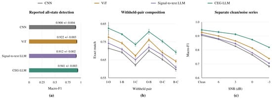
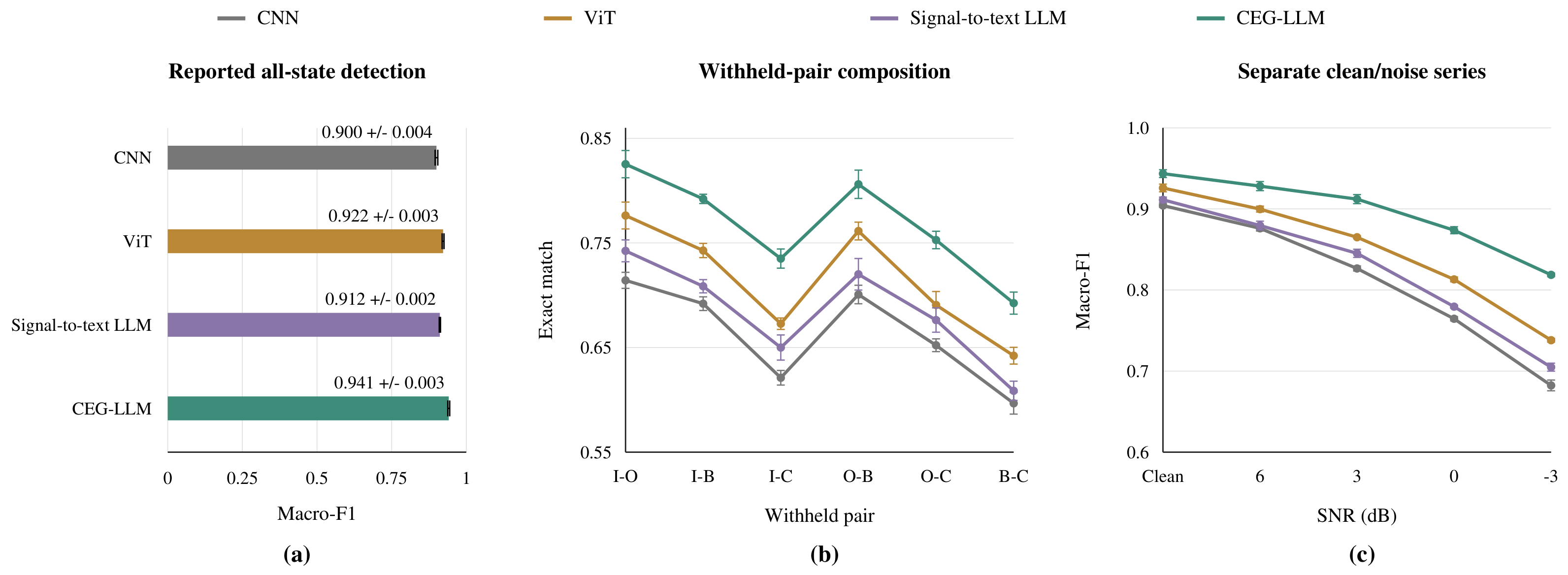
In observed-state detection, CEG-LLM achieved a mean macro-F1 of 0.941, compared with 0.922 for ViT (Figure 5a). The signal-to-text language encoder and CNN achieved 0.912 and 0.900, respectively. The CEG-LLM minus ViT difference was 0.019, equivalent to 1.9 percentage points.
Figure 5.
Detection performance and sensitivity to additive noise in the bearing evaluation. (a) Comparison of observed-state macro-F1 across different methods; (b) Exact-match performance on six withheld defect pairs; (c) Macro-F1 comparison under different SNRs.
Across the six withheld pairs, CEG-LLM achieved a mean exact match of 0.767, compared with 0.714 for ViT (Figure 5b). Corresponding means were 0.684 for the signal-to-text language encoder and 0.663 for CNN. The CEG-LLM minus ViT difference was approximately 0.053. CEG-LLM obtained its highest scores for I-O and O-B, while B-C and I-C were more difficult. CNN and ViT showed a similar ranking for cage-related pairs despite not using the proposed anchors. This common ranking cannot be attributed specifically to the masked CEG-LLM cage anchor. Cage-signal properties and dataset characteristics remain possible explanations that the aggregate results cannot distinguish.
Performance decreased from the clean condition to dB in the noise evaluation. Clean-condition means were 0.904 for CNN, 0.926 for ViT, 0.911 for the signal-to-text language encoder, and 0.944 for CEG-LLM. This separately indexed evaluation differs slightly from the observed-state summary, as distinguished in Table 2. At dB, the respective means were 0.682, 0.738, 0.705, and 0.819. Within this series, the clean-to- dB decreases were 0.18776 for ViT and 0.12482 for CEG-LLM. Because ViT also uses local patches, the smaller decrease characterizes the complete CEG-LLM method rather than patch-based encoding alone.
Table 3 presents the mean for each of the six withheld pairs. The CEG-LLM minus ViT differences computed from the rounded means were 0.049, 0.049, and 0.062 for I-O, I-B, and I-C, respectively. The corresponding differences were 0.045, 0.062, and 0.050 for O-B, O-C, and B-C. Their descriptive mean was 0.0528, with a range of 0.045 to 0.062. The lowest CEG-LLM exact match was 0.692 for the B-C pair. These pair-level comparisons use fold means without assuming independent folds or providing a paired p-value.
Table 3.
Withheld-pair exact match as mean across five seeds per pair.
4.3. Calibration, Evidence Sensitivity, and Ablation
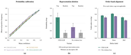
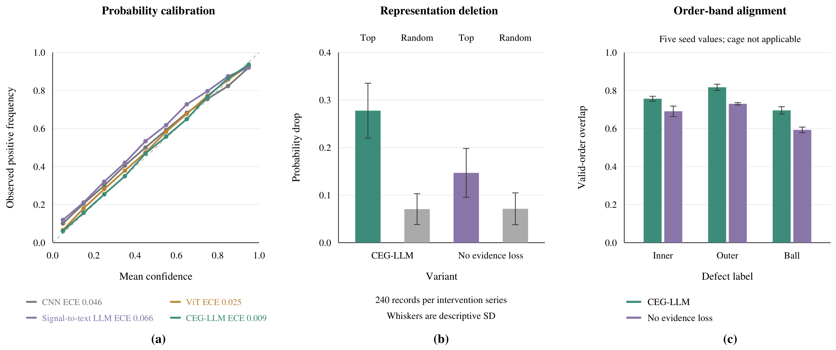
Calibration was evaluated independently of accuracy using mean confidence, observed positive frequency, and count for each reliability bin. Count-weighted absolute gaps gave ECE values of 0.009 for CEG-LLM, 0.025 for ViT, 0.046 for CNN, and 0.066 for the signal-to-text language encoder. Figure 6a presents the reliability curves and their ECE values. Differences in bin counts explain why similar high-confidence curves can yield different overall calibration errors.
Figure 6.
Calibration and attribution results from the bearing evaluation. (a) Probability calibration curves and ECEs across different methods; (b) Comparison of prediction probability drops under top-evidence and random-token deletion; (c) Comparison of valid-order overlap across defect labels with and without evidence loss.
Mean deletion contrast was 0.207 for the full model and 0.076 without evidence loss, giving a difference of 0.131. The full model’s mean valid-order overlap was 0.757 across the evaluated I/O/B channels. These measures assess representation sensitivity and alignment with the chosen order library, respectively.
Table 4 summarizes three individual component removals and two input or encoder substitutions. Removing physical anchors reduced macro-F1 from 0.941 to 0.924 and deletion contrast from 0.207 to 0.139. Removing the graph-conditioned module reduced withheld-pair exact match to 0.701, the largest decrease among the single-component removals. Global statistics and the compact encoder yielded lower exact-match values of 0.642 and 0.689, respectively, but involved broader input or encoder changes. Removing the evidence loss retained a macro-F1 of 0.937 while reducing deletion contrast to 0.076. Classification accuracy and representation sensitivity thus responded differently to this regularizer.
Table 4.
Ablation means across five seeds.
The compact encoder achieved 0.915 macro-F1 and 0.689 exact match, below ViT’s 0.922 and 0.714 despite retaining the proposed task components. Physical descriptors and graph conditioning alone therefore do not explain the full-model advantage. The full model exceeded the compact variant by 0.026 in macro-F1 and 0.078 in exact match.
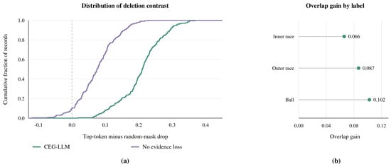
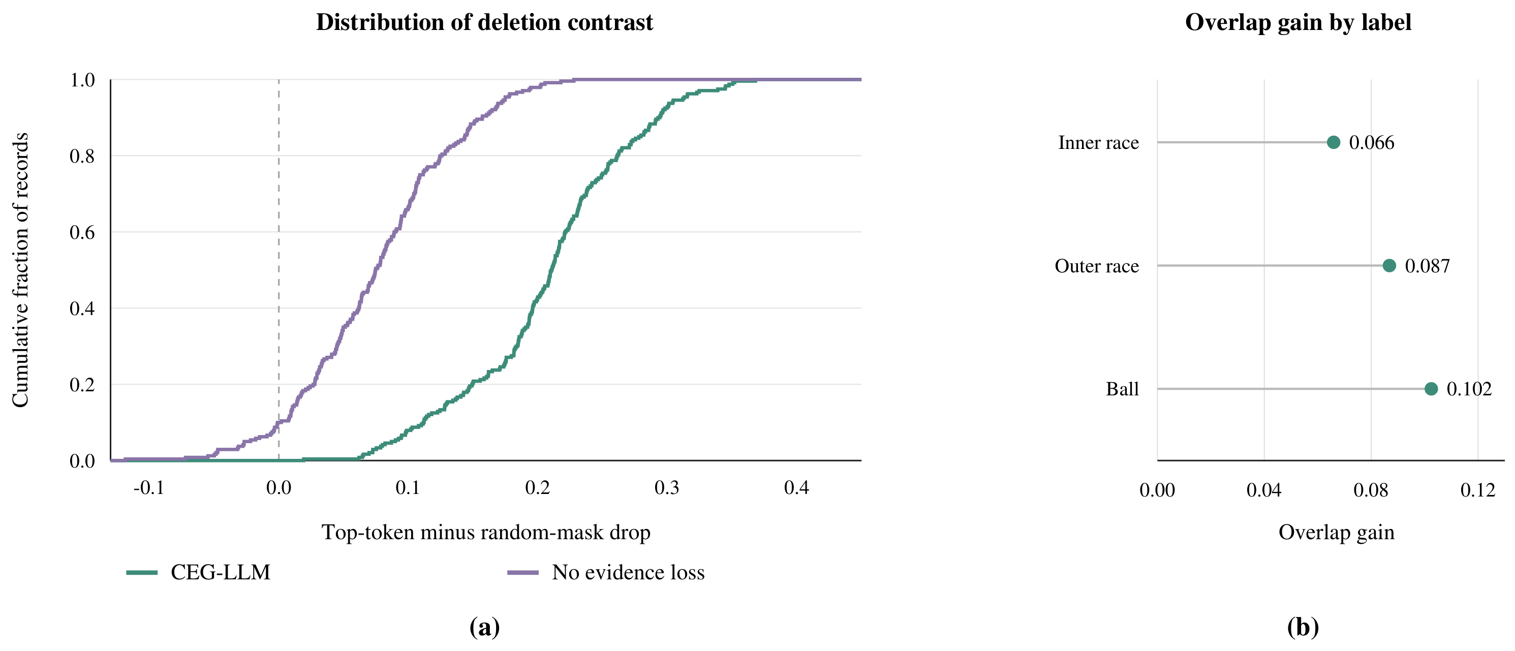
Figure 7 summarizes 240 paired top-token and random-mask intervention records per variant. Mean and median deletion contrasts were 0.20705 and 0.21060 for the full model, compared with 0.07558 and 0.07464 without evidence loss. The fractions of records with positive contrast were 1.000 and 0.900, respectively. These are descriptive summaries of intervention records and do not represent 240 independent experiments. The I/O/B overlap gains were 0.066, 0.087, and 0.102, respectively.
Figure 7.
Distribution of deletion contrasts and comparison of order alignment. (a) Cumulative distributions of deletion contrasts for CEG-LLM and the variant without evidence loss; (b) Valid-order overlap gains across different defect labels.
5. Discussion
5.1. Compositional Representation and Practical Interpretation
The formulation represents compound defects in rotating components through four atomic labels and links each prediction to an inspectable signal record. This separates the representation of defect types from the enumeration of their combinations, allowing known types to be recognized together without a new class. In practice, a report identifying I and B with their scores and token origins can guide inspection of the corresponding component locations. The report remains a diagnostic aid whose interpretation depends on the available signal evidence. An unresolved cage anchor, a shared harmonic, or an ambiguous quality flag warrants review of a longer signal record before a maintenance decision.
The ablations indicate that the encoder and task modules contribute differently to the evaluated quantities. Among single-component removals, excluding the graph module most reduces withheld-pair exact match, while excluding the evidence loss most reduces deletion contrast. Graph conditioning therefore contributes to compositional recognition, while the evidence objective influences sensitivity to selected representations. However, the graph is fully connected, and the compact encoder performs below the plain ViT. The observed advantage consequently cannot be attributed predominantly to physical descriptors or graph topology alone.
5.2. Attention and Physical Evidence
A token-origin record identifies the interval used to construct a token, while the final hidden state combines information across positions. Label attention visualizes the decoder readout but does not decompose the waveform into physical causes. A positive deletion contrast indicates greater prediction sensitivity to the selected representation than to a size-matched random control under the specified intervention. Distribution shifts induced by masking limit the interpretation of this comparison. Signal-origin tracking, representation sensitivity, and physical causality must therefore be distinguished when assessing the evidence associated with a prediction.
Cage detection illustrates how observation duration limits the available physical evidence. With the stated nominal geometry, a window covers less than one cage revolution, so the cage anchor and its evidence-loss term are masked. A positive cage output can still depend on waveform patterns and contextual features, although it lacks a resolved cage-frequency trace. I-C and B-C are also relatively difficult for CNN and ViT. This common ranking cannot be assigned solely to the proposed anchor mask and may reflect cage-signal observability or interactions among defect responses.
6. Conclusions
CEG-LLM formulates compound defect detection in rotating components as compositional multi-label learning using atomic labels, tokens with recorded origins, and graph-conditioned language-encoder representations. Spectral alignment and compositional regularization connect this formulation to the available physical cues and combinations of known defect types. The full model achieved higher mean detection and withheld-pair recognition scores than the evaluated baselines on the dataset collected from a rotating component at fixed speed. The ablations distinguish the contributions to classification, compositional recognition, and representation sensitivity. These findings support the evaluated formulation within the present dataset, while the evidence records remain subject to frequency-resolution and attribution limits.
Further work may aggregate evidence over longer temporal contexts for cage-related outputs and adapt order descriptions to changing operating conditions. More compact signal encoders may also reduce the processing cost of continuous monitoring. These directions address the distinct limits of short-window recognition, physical-order observability, and computational cost.
Author Contributions
Conceptualization, X.Z. and Z.W.; Methodology, X.Z. and Z.W.; Validation, X.Z.; Formal Analysis, M.W., M.C., H.Z., J.C. and Z.W.; Data Curation, X.Z., M.W. and M.C.; Writing (Original Draft), X.Z.; Writing (Review and Editing), X.Z., M.W., H.Z. and Z.W.; Visualization, X.Z., M.W., M.C., H.Z. and J.C.; Supervision, Z.W. All authors have read and agreed to the published version of the manuscript.
Funding
This research received no external funding.
Data Availability Statement
The datasets presented in this article are not readily available because the industrial data are obtained from an enterprise’s real platform and subject to confidentiality constraints. The data presented in this study are available on request from the corresponding author.
Acknowledgments
During the preparation of this manuscript, the authors used ChatGPT (GPT-5.6 Sol) solely for grammar and language editing. The authors reviewed and edited the output and take full responsibility for the content of this publication.
Conflicts of Interest
The authors declare no conflicts of interest.
References
- Xu, Z.; Jia, Z.; Wei, Y.; Zhang, S.; Jin, Z.; Dong, W. A strong anti-noise and easily deployable bearing fault diagnosis model based on time-frequency dual-channel Transformer. Measurement 2024, 236, 115054. [Google Scholar] [CrossRef] [Scilit]
- Chu, L.; Li, Q.; Yang, B.; Chen, L.; Shen, C.; Wang, D. Exploring the essence of compound fault diagnosis: A novel multi-label domain adaptation method and its application to bearings. Heliyon 2023, 9, e14545. [Google Scholar] [CrossRef] [Scilit] [PubMed]
- Jin, Y.; Qin, C.; Zhang, Z.; Tao, J.; Liu, C. A multi-scale convolutional neural network for bearing compound fault diagnosis under various noise conditions. Sci. China Technol. Sci. 2022, 65, 2551–2563. [Google Scholar] [CrossRef] [Scilit]
- Liao, J.X.; He, C.; Li, J.; Sun, J.; Zhang, S.; Zhang, X. Classifier-guided neural blind deconvolution: A physics-informed denoising module for bearing fault diagnosis under noisy conditions. Mech. Syst. Signal Process. 2025, 222, 111750. [Google Scholar] [CrossRef] [Scilit]
- Liu, B.; Yan, C.; He, C.; Lv, M.; Wei, J.; Wu, L. An Interpretable Physics-Informed Subdomain Moment-Enhanced Adaptation Network for Unsupervised Transfer Fault Diagnosis of Rolling Bearing. Adv. Eng. Inform. 2025, 67, 103491. [Google Scholar] [CrossRef] [Scilit]
- Dong, X.; Niu, G.; Wang, H.; Oh, H. Convenient Gearbox Fault Diagnosis Under Random Variable Speeds: A Motor Current Nonlinear Harmonic Approach. Mech. Syst. Signal Process. 2025, 225, 112290. [Google Scholar] [CrossRef] [Scilit]
- Chen, Y.; Li, Z.; Jiang, Y.; Gong, D.; Zhou, K. Sparse LPV–ARMA Model for Non-Stationary Vibration Representation and Its Application on Gearbox Tooth Crack Detection Under Variable Speed Conditions. Mech. Syst. Signal Process. 2025, 224, 112161. [Google Scholar] [CrossRef] [Scilit]
- Liu, B.; Yan, C.; Liu, Y.; Lv, M.; Huang, Y.; Wu, L. ISEANet: An Interpretable Subdomain Enhanced Adaptive Network for Unsupervised Cross-Domain Fault Diagnosis of Rolling Bearing. Adv. Eng. Inform. 2024, 62, 102610. [Google Scholar] [CrossRef] [Scilit]
- Zhang, Y.; Ji, J.C.; Ren, Z.; Ni, Q.; Wen, B. Multi-sensor open-set cross-domain intelligent diagnostics for rotating machinery under variable operating conditions. Mech. Syst. Signal Process. 2023, 191, 110172. [Google Scholar] [CrossRef] [Scilit]
- Wang, R.; Huang, W.; Lu, Y.; Wang, J.; Ding, C.; Liao, Y.; Shi, J. Cloud-edge collaborative transfer fault diagnosis of rotating machinery via federated fine-tuning and target self-adaptation. Expert Syst. Appl. 2024, 250, 123859. [Google Scholar] [CrossRef] [Scilit]
- Zhu, M.; Liu, J.; Hu, Z.; Liu, J.; Jiang, X.; Shi, T. Cloud-Edge Test-Time Adaptation for Cross-Domain Online Machinery Fault Diagnosis via Customized Contrastive Learning. Adv. Eng. Inform. 2024, 61, 102514. [Google Scholar] [CrossRef] [Scilit]
- Feng, J.; Bao, S.; Xu, X.; Zhang, Z.; Hou, P.; Steyskal, F.; Dustdar, S. Rotating machinery fault diagnosis based on feature extraction via an unsupervised graph neural network. Appl. Intell. 2023, 53, 21211–21226. [Google Scholar] [CrossRef] [Scilit]
- Weng, C.; Lu, B.; Chen, L.; Zhao, X.; Huang, W. A novel progressive domain separation network with multi-metric ensemble quantification for open set fault diagnosis of motor bearings. Adv. Eng. Inform. 2025, 64, 103060. [Google Scholar] [CrossRef] [Scilit]
- Wang, Z.; Xuan, J.; Shi, T. An autonomous recognition framework based on reinforced adversarial open set algorithm for compound fault of mechanical equipment. Mech. Syst. Signal Process. 2024, 219, 111596. [Google Scholar] [CrossRef] [Scilit]
- Qin, Y.; Liu, X.; Li, X.; Mao, Y. Simulation-data driven generalized zero-shot learning for multi-agent bearing compound fault diagnosis. Knowl.-Based Syst. 2025, 318, 113595. [Google Scholar] [CrossRef] [Scilit]
- Jiao, S.; Ning, S.; Zhu, X.; Liu, Y.; Zhang, R.; Karimi, H.R. Zero-shot bearing diagnosis via semantic prototype synthesis: From single to compound faults. Struct. Health Monit. 2026. [Google Scholar] [CrossRef] [Scilit]
- Ma, C.; Wang, X.; Li, Y.; Cai, Z. Broad zero-shot diagnosis for rotating machinery with untrained compound faults. Reliab. Eng. Syst. Saf. 2024, 242, 109704. [Google Scholar] [CrossRef] [Scilit]
- Xing, S.; Lei, Y.; Wang, S.; Lu, N.; Li, N. A label description space embedded model for zero-shot intelligent diagnosis of mechanical compound faults. Mech. Syst. Signal Process. 2022, 162, 108036. [Google Scholar] [CrossRef] [Scilit]
- Chen, H.; Hong, J.; Cheng, C.; Kong, Y.; Zheng, X. Zero-Shot Compound Fault Diagnosis Method Using Semantic Construction and Embedding. IEEE Trans. Instrum. Meas. 2024, 73, 1–13. [Google Scholar] [CrossRef] [Scilit]
- Wang, J.; Xu, Z.; Niu, F.; Liu, J.; Zhu, Z. Adaptively Weighted Semantic Autoencoder for Zero-Shot Compound Fault Diagnosis. IEEE Sens. J. 2024, 24, 37472–37481. [Google Scholar] [CrossRef] [Scilit]
- Oh, H.I.; Jung, J.H. A Generalized Zero-Shot Learning Framework for Bearing Compound Fault Diagnosis Using a Class-Aware VAE-Based Semantic Vector Extractor. Mech. Syst. Signal Process. 2026, 255, 114370. [Google Scholar] [CrossRef] [Scilit]
- Xu, J.; Li, K.; Fan, Y.; Yuan, X. A Label Information Vector Generative Zero-Shot Model for the Diagnosis of Compound Faults. Expert Syst. Appl. 2023, 233, 120875. [Google Scholar] [CrossRef] [Scilit]
- Shang, Z.; Tang, L.; Pan, C.; Cheng, H. A Hybrid Semantic Attribute-Based Zero-Shot Learning Model for Bearing Fault Diagnosis Under Unknown Working Conditions. Eng. Appl. Artif. Intell. 2024, 136, 109020. [Google Scholar] [CrossRef] [Scilit]
- Zhu, Q.; Liu, H.; Bao, C.; Zhu, J.; Mao, X.; He, S.; Peng, F. Decoupled Interpretable Robust Domain Generalization Networks: A Fault Diagnosis Approach Across Bearings, Working Conditions, and Artificial-to-Real Scenarios. Adv. Eng. Inform. 2024, 61, 102445. [Google Scholar] [CrossRef] [Scilit]
- Xu, C.; Wang, Z.; Jin, Y.; Nong, W. An adaptive industrial large language model for mechanical fault diagnosis under variable operating conditions. Adv. Eng. Inform. 2026, 74, 104821. [Google Scholar] [CrossRef] [Scilit]
- Li, D.; Pang, Z.; Chen, Y.; Yang, K.; Shao, J.; Luo, Y.; Zeng, Y.; He, C.; Gao, Y. FD-MVLLM: Fault diagnosis based on multimodal vibration data and large language model for bearing system. Mech. Syst. Signal Process. 2025, 239, 113226. [Google Scholar] [CrossRef] [Scilit]
- Qaid, H.A.A.M.; Zhang, B.; Su, S.; Li, D.; Ng, S.K.; Li, W. Large language models for explainable fault diagnosis of machines. Eng. Appl. Artif. Intell. 2026, 163, 113131. [Google Scholar] [CrossRef] [Scilit]
- Lin, L.; Zhang, S.; Fu, S.; Liu, Y. FD-LLM: Large Language Model for Fault Diagnosis of Complex Equipment. Adv. Eng. Inform. 2025, 65, 103208. [Google Scholar] [CrossRef] [Scilit]
- Zhang, C.; Wang, Y.; You, X. Fault diagnosis in rotating machinery with discretized signal representation leveraging large language models. Appl. Soft Comput. 2026, 189, 114487. [Google Scholar] [CrossRef] [Scilit]
- Zhang, Q.; Xu, C.; Li, J.; Sun, Y.; Bao, J.; Zhang, D. LLM-TSFD: An Industrial Time Series Human-in-the-Loop Fault Diagnosis Method Based on a Large Language Model. Expert Syst. Appl. 2025, 264, 125861. [Google Scholar] [CrossRef] [Scilit]
- Wang, Z.; Chen, J.; Wang, C.; Peng, C.; Xuan, J.; Shi, T.; Zuo, M. CNC-VLM: An RLHF-optimized industrial large vision-language model with multimodal learning for imbalanced CNC fault detection. Mech. Syst. Signal Process. 2026, 245, 113838. [Google Scholar] [CrossRef] [Scilit]
- Guo, J.; He, Q.; Zhen, D.; Gu, F.; Ball, A.D. Multi-sensor data fusion for rotating machinery fault detection using improved cyclic spectral covariance matrix and motor current signal analysis. Reliab. Eng. Syst. Saf. 2023, 230, 108969. [Google Scholar] [CrossRef] [Scilit]
- Tian, S.; Zhen, D.; Li, H.; Feng, G.; Zhang, H.; Gu, F. Adaptive Resonance Demodulation Semantic-Induced Zero-Shot Compound Fault Diagnosis for Railway Bearings. Measurement 2024, 235, 115040. [Google Scholar] [CrossRef] [Scilit]
- Qin, Y.; Zhao, L.; Chen, Y.; Xiao, D.; Mao, Y. Learnable Wavelet-Driven Physically Interpretable Networks for Bearing Fault Diagnosis Under Variable Speed. Mech. Syst. Signal Process. 2025, 237, 113121. [Google Scholar] [CrossRef] [Scilit]
- Wang, Z.; Xuan, J.; Shi, T.; Li, Y.F. Multi-label domain adversarial reinforcement learning for unsupervised compound fault recognition. Reliab. Eng. Syst. Saf. 2025, 254, 110638. [Google Scholar] [CrossRef] [Scilit]
- Chen, P.; Zhao, R.; He, T.; Wei, K.; Yuan, J. A novel bearing fault diagnosis method based joint attention adversarial domain adaptation. Reliab. Eng. Syst. Saf. 2023, 237, 109345. [Google Scholar] [CrossRef] [Scilit]
- Wang, Z.; Li, S.; Xuan, J.; Shi, T. Biologically inspired compound defect detection using a spiking neural network with continuous time–frequency gradients. Adv. Eng. Inform. 2025, 65, 103132. [Google Scholar] [CrossRef] [Scilit]
- Xu, J.; Liang, S.; Ding, X.; Yan, R. A Zero-Shot Fault Semantics Learning Model for Compound Fault Diagnosis. Expert Syst. Appl. 2023, 221, 119642. [Google Scholar] [CrossRef] [Scilit]
- Xia, H.; Meng, T.; Zuo, Z.; Ma, W. Fault semantic knowledge transfer learning: Cross-domain compound fault diagnosis method under limited single fault samples. Reliab. Eng. Syst. Saf. 2025, 260, 111050. [Google Scholar] [CrossRef] [Scilit]
- Xu, J.; Kong, H.; Li, K.; Ding, X. Generative Zero-Shot Compound Fault Diagnosis Based on Semantic Alignment. IEEE Trans. Instrum. Meas. 2024, 73, 1–13. [Google Scholar] [CrossRef] [Scilit]
- Wang, L.; Chen, D.; Mao, Y.; Qin, Y. A Zero-Shot Attribute-Embedded Model With a Feature Difference Mapping Sigmoid Function for Compound Fault Diagnosis of Rotating Machinery. ISA Trans. 2025, 157, 451–465. [Google Scholar] [CrossRef] [Scilit] [PubMed]
- Qin, Y.; Wang, L.; Qian, Q.; Mao, Y. Zero-Shot Attribute Consistent Model for Bearing Fault Diagnosis Under Unknown Domain. IEEE Trans. Instrum. Meas. 2024, 73, 1–11. [Google Scholar] [CrossRef] [Scilit]
- Read, J.; Pfahringer, B.; Holmes, G.; Frank, E. Classifier chains for multi-label classification. Mach. Learn. 2011, 85, 333–359. [Google Scholar] [CrossRef] [Scilit]
- NSK. 6200 Single-Row Deep Groove Ball Bearings. 2026. Available online: https://www.nsk.com/engineering/products/bearings/ball-bearings/deep-groove-ball-bearings/single-row-deep-groove-ball-bearings/6200-apn.html (accessed on 9 October 2026).
- Jain, S.; Wallace, B.C. Attention is not Explanation. In Proceedings of the NAACL-HLT, Minneapolis, MN, USA, 2–7 June 2019; pp. 3543–3556. [Google Scholar] [CrossRef] [Scilit]
- Hooker, S.; Erhan, D.; Kindermans, P.J.; Kim, B. A Benchmark for Interpretability Methods in Deep Neural Networks. In Proceedings of the Advances in Neural Information Processing Systems, Vancouver, BC, Canada, 8–14 December 2019; Volume 32. Available online: https://proceedings.neurips.cc/paper_files/paper/2019/hash/fe4b8556000d0f0cae99daa5c5c5a410-Abstract.html (accessed on 10 November 2026).

Disclaimer/Publisher’s Note: The statements, opinions and data contained in all publications are solely those of the individual author(s) and contributor(s) and not of MDPI and/or the editor(s). MDPI and/or the editor(s) disclaim responsibility for any injury to people or property resulting from any ideas, methods, instructions or products referred to in the content. |
© 2026 by the authors. Licensee MDPI, Basel, Switzerland. This article is an open access article distributed under the terms and conditions of the Creative Commons Attribution (CC BY) license.