A Formal Correspondence Between Bayesian Inference Problems and the Heisenberg Representation

Abstract

The proposed formulation establishes a formal correspondence between the Heisenberg representation and the Bayesian formulation of inverse problems. The likelihood function is first expressed in a Hilbert space through a quadratic norm of the difference between noisy observations and the response of a forward model depending on the unknown parameters $\mathit{\nu }$, weighted by the inverse of the observational noise covariance. Based on the common mathematical structure of this quadratic form and an operator expectation value, the inverse observational noise covariance operator is identified, as a modeling hypothesis, with the initial observable $\widehat{A}(\mathbf{s},0)\equiv {\mathsf{\Gamma }}_{\mathrm{noise}}^{-1}$. To establish this correspondence, a stochastic field with Matérn covariance C is considered and represented through the Karhunen–Loève expansion. The eigenvalues and eigenfunctions of this expansion are then used to define the state $|\mathsf{\Psi }⟩$ within the proposed formalism and to construct the Hamiltonian governing the Heisenberg evolution. The main theorem formalizes the correspondence between the Bayesian likelihood and the initial Heisenberg observable under this modeling hypothesis. Limiting cases of the Matérn covariance are analyzed as $\ell \to 0$ and $\ell \to \infty$. Finally, numerical examples illustrate a non-trivial Heisenberg evolution, verify the invariance of the observable trace, and demonstrate the numerical equivalence between the Bayesian likelihood and the Heisenberg representation in the Karhunen–Loève basis, including standard and hierarchical Bayesian benchmarks.

1. Introduction

Inverse methods have become an essential tool in different fields of science and engineering, such as geophysics [1,2], biomechanics, materials engineering, and medical tomography [3,4], among others [5]. The aim of these methods is to estimate unknown parameters, such as the physical or geometric properties of a medium or anomaly, from generally noisy observations [4]. There are multiple approaches to addressing inverse problems, from deterministic methods such as the Levenberg-Marquardt minimization method [6,7], to probabilistic methods such as Bayesian inference [4,8]. In the Bayesian approach, the posterior distribution $f_{\mathrm{post}}\left(\mathit{\nu }\right)$ of the unknown parameter $\mathit{\nu }$ is obtained using Bayes’s theorem by combining the prior distribution and the likelihood function [8].

In this paper, both the prior distribution and the likelihood are assumed to be Gaussian, a choice widely used in the literature [9]. Under this assumption, the posterior distribution is expressed as an exponential whose argument is the sum of two quadratic terms: one corresponding to the residual between the observed noisy data and the forward model prediction, and the other associated with the deviation of the unknown parameter from its prior mean [8]. The likelihood function is typically expressed in terms of the weighted Euclidean distance between the observed noisy data ${\mathbf{d}}^{obs}$ and the model response $\mathbf{f}\left(\mathit{\nu }\right)$, with weighting determined by the inverse observational noise covariance [8,9].

This formulation is natural in the Hilbert space of square-integrable functions, where the weighted Euclidean norm can be expressed in terms of an inner product induced by the inverse observational noise covariance operator ${\mathsf{\Gamma }}_{\mathrm{noise}}^{-1}$[10]. However, in practical Bayesian inverse problems, the observational noise covariance ${\mathsf{\Gamma }}_{\mathrm{noise}}$ may be unknown or only partially characterized. This provides additional motivation for studying an alternative mathematical representation of the observational noise structure, although the estimation of a fully unknown covariance operator is beyond the scope of the present work.

Recent works have investigated the role of observation operators in Bayesian inverse problems, analyzing how their choice can mitigate the effect of model error on the posterior distribution [11]. Another recent study considers linear Bayesian inverse problems in Hilbert spaces in which the forward operator and the prior covariance operator are not assumed to commute [12]. This work illustrates that non-commuting operators can arise naturally in the analysis of Bayesian inverse problems. The present work considers a different operator connection: the inverse observational noise covariance ${\mathsf{\Gamma }}_{\mathrm{noise}}^{-1}$ is identified with the initial observable of a Heisenberg evolution.

This paper proposes a formal correspondence between Bayesian inference and the Heisenberg representation. In the proposed formulation, the residual between the noisy observational data and the forward response is represented in the Karhunen–Loève (KL) basis, while the inverse observational noise covariance is introduced as the initial observable of the Heisenberg representation. The same KL spectral structure is used to represent the stochastic field and later, to construct the Hamiltonian governing the unitary evolution of the observable. This places the Bayesian weighted quadratic form and the Heisenberg evolution in the same operator framework.

The aim of this work is to establish a formal operator correspondence, not to introduce a new Bayesian estimator or inference algorithm. In particular, the inverse observational noise covariance ${\mathsf{\Gamma }}_{\mathrm{noise}}^{-1}$ is introduced through the modeling hypothesis $\widehat{A}(\mathbf{s},0)\equiv {\mathsf{\Gamma }}_{\mathrm{noise}}^{-1}$. The proposed construction does not imply quantization of the underlying physical inverse problem; the Heisenberg representation is used here as a mathematical operator framework.

Theorem 1 establishes the formal correspondence between the quadratic form of the Bayesian likelihood and the Heisenberg representation in the KL basis. In addition, the limiting cases of the Matérn covariance for $\ell \to 0$ and $\ell \to \infty$ are analyzed to characterize vanishing and long range correlation regimes.

The article is organized as follows. In Section 2, the necessary mathematical preliminaries are presented, including Hilbert space, Fock space, the Matérn covariance operator, and the Karhunen–Loève expansion. In Section 3, the Hamiltonian of the system is constructed in Fock space. In Section 4, the formulation of the state $|\mathsf{\Psi }⟩$ written as a stochastic field based on the KL basis is established. In Section 5, the evolution of an observable in the Heisenberg representation is studied, and its expected value is defined. Section 6 links the proposed formalism with Bayesian inference, and introduces the modeling hypothesis $\widehat{A}(\mathbf{s},0)\equiv {\mathsf{\Gamma }}_{\mathrm{noise}}^{-1}$. Section 7 presents the three structural propositions that provide the mathematical framework for the main theorem, followed by the analysis of the limiting cases of the Matérn covariance. Section 8 presents numerical examples illustrating the analytical results. Finally, Section 9 presents the conclusions and discusses possible directions for future research.

2. Mathematical Prerequisites

2.1. Hilbert Space of Functions

A Hilbert space is a real or complex inner product space that is complete with respect to the norm induced by the inner product [10].

In this paper, the Hilbert space of interest is the space of square-integrable functions $L^2\left(\mathsf{\Omega }\right)$, where $\mathsf{\Omega }=D\times I$, with $D\subset {\mathbb{R}}^N$ the spatial domain and $I=[0,T]$ the time domain [13]. The inner product in $L^2\left(\mathsf{\Omega }\right)$ is defined as

$$⟨f|g⟩={\int }_{\mathsf{\Omega }}d\mathbf{s}dt{f}^{*}(\mathbf{s},t)g(\mathbf{s},t),$$

and the associated norm is

$$\parallel f\parallel ={\left({\int }_{\mathsf{\Omega }}d\mathbf{s}dt{\left|f(\mathbf{s},t)\right|}^2\right)}^{1/2}.$$

This space provides the natural framework for the study of stochastic fields and integral operators, such as those appearing in the Karhunen–Loève expansion [14] and operator representations used in this work [15].

2.2. Fock Space and Second Quantization

2.2.1. Fock Space

In quantum mechanics, Fock space is a special Hilbert space constructed as the direct sum of tensor products (symmetrized or antisymmetrized) of another Hilbert space for a single particle [16]. This space is used to describe the state of a system consisting of a variable or indeterminate number of particles.

Fock space can be described using an occupation number basis, in which each basis vector specifies the occupation numbers associated with the available modes [15]. As in Hilbert space, Fock space contains creation operators $a_i^{†}$, which add a particle to state i, and annihilation operators $a_i$, which remove a particle from state i [17]. In the bosonic Fock space representation adopted in this work, the creation and annihilation operators satisfy [15],

$$[a_i,a_j^{†}]={\delta }_{ij},[a_i,a_j]=0,[a_i^{†},a_j^{†}]=0.$$

The Fock space formulation allows the field to be described using creation and annihilation operators associated with the Karhunen–Loève modes.

2.2.2. Second Quantization

Second quantization is a formulation that allows us to describe systems with a variable number of particles, in contrast to first quantization, which deals with systems of individual particles [17,18].

In quantum field theory, particles are viewed as excitations of quantum fields [18]. One of the characteristics of second quantization is that fields are transformed into operators acting on Fock space, which contains all possible states of the system with different numbers of particles; this allows us to describe processes in which particles are created or annihilated. This formalism provides a framework for describing many-particle systems. Second quantization allows us to interpret quantum fields in terms of particles. Each state can be interpreted as a vector in Fock space [19]. A state can be represented as a superposition of states with an integer number of quanta associated with the field, each having a well-defined energy [16].

In the context of this work, second quantization allows the modes of the Karhunen–Loève expansion to be represented by creation and annihilation operators. Each eigenfunction ${\varphi }_i$ of the Matérn covariance is associated with an occupation mode, and the corresponding field operators are expanded in the same spectral basis. This construction is used in Section 3 to define the Hamiltonian.

Although the construction of the Fock space is not required for the Bayesian likelihood itself, its role in this work is to provide the second quantized operator setting in which the Hamiltonian governing the Heisenberg evolution is constructed. The Fock space does not constitute an alternative Bayesian inference procedure; rather it provides the operator framework in which the initial observable is embedded and subsequently evolved according to the Heisenberg representation.

2.3. Matérn Kernel

Consider a stochastic field $u(\mathbf{s},t;\alpha )$, where the spatial dependence is given by $\mathbf{s}\in {\mathbb{R}}^N$ and the temporal dependence by $t>0$. The Whittle-Matérn stochastic differential equation that generates the field $u(\mathbf{s},t;\alpha )$ for each realization $\alpha$ is [20,21],

$${\displaystyle \frac{1}{\sqrt{\beta }}}{(I-{\ell }_s^2\Delta )}^{(\eta +{\displaystyle \frac{N}{2}})/2}{(I-{\ell }_t^2{\displaystyle \frac{{\partial }^2}{\partial t^2}})}^{({\eta }_t+{\displaystyle \frac{1}{2}})/2}u(\mathbf{s},t;\alpha )=W(\mathbf{s},t),$$

(1)

where $\Delta$ is the Laplacian operator, ${\displaystyle \frac{{\partial }^2}{\partial t^2}}$ is the second-order time derivative, $\eta >0$ is the spatial smoothing factor, ${\eta }_t>0$ is the temporal smoothing factor, ${\ell }_s$ and ${\ell }_t$ are the spatial and temporal length-scale parameters, respectively. In Equation (1), $W(\mathbf{s},t)$ is a Gaussian white noise process with unit variance and mean zero and $\beta$ is a constant that depends on the parameters of the Matérn kernel.

The spectral density $S_u(\mathbf{k},\omega )$ of the field $u(\mathbf{s},t;\alpha )$ is defined as

$$S_u(\mathbf{k},\omega )={\displaystyle \frac{\beta \mathbb{E}[|\widehat{W}(\mathbf{k},\omega ){|}^2]}{{\left(1+{\ell }_s^2{\left|\mathbf{k}\right|}^2\right)}^{\eta +N/2}{\left(1+{\ell }_t^2{\omega }^2\right)}^{{\eta }_t+1/2}}},$$

(2)

where $\mathbf{k}$ is the wave vector, $\omega$ is the temporal frequency and $E[|\widehat{W}(\mathbf{k},\omega ){|}^2]=1$. The Equation (2) allows the spectral density to be written as the product of the spatial spectral density $S_{\mathbf{s}}={\displaystyle \frac{1}{{\left(1+{\ell }_s^2{\left|\mathbf{k}\right|}^2\right)}^{\eta +N/2}}}$ with the temporal spectral density $S_t={\displaystyle \frac{1}{{\left(1+{\ell }_t^2{\omega }^2\right)}^{{\eta }_t+1/2}}}$. Therefore, the spectral density can be written as

$$S_u(\mathbf{k},\omega )=\beta S_{\mathbf{s}}\left(\mathbf{k}\right)S_t\left(\omega \right).$$

(3)

From this spectral density, the covariance is obtained using the inverse Fourier transform, that is,

$$C(\mathbf{s},{\mathbf{s}}^{\prime },t,t^{\prime })={\left(2\pi \right)}^{-(N+1)}{\int }_{\mathbb{R}}{\int }_{{\mathbb{R}}^N}{S}_u(\mathbf{k},\omega )\exp (-i[\mathbf{k}·(\mathbf{s}-{\mathbf{s}}^{\prime })-\omega (t-t^{\prime })])d\mathbf{k}d\omega .$$

(4)

Taking the inverse Fourier transform in Equation (4) yields the following Matérn-type space-time covariance,

$$C(\mathbf{s},{\mathbf{s}}^{\prime },t,t^{\prime })={\sigma }_u^2{\displaystyle \frac{2^{1-\eta }}{\mathsf{\Gamma }\left(\eta \right)}}{\left({\displaystyle \frac{\left|\right|\mathbf{s}-{\mathbf{s}}^{\prime }\left|\right|}{{\ell }_s}}\right)}^{\eta }{K}_{\eta }\left({\displaystyle \frac{\left|\right|\mathbf{s}-{\mathbf{s}}^{\prime }\left|\right|}{{\ell }_s}}\right){\displaystyle \frac{2^{1-{\eta }_t}}{\mathsf{\Gamma }\left({\eta }_t\right)}}{\left({\displaystyle \frac{|t-t^{\prime }|}{{\ell }_t}}\right)}^{{\eta }_t}{K}_{{\eta }_t}\left({\displaystyle \frac{|t-t^{\prime }|}{{\ell }_t}}\right),$$

(5)

where $K_{\eta }$ and $K_{{\eta }_t}$ are modified Bessel functions of the second kind of orders $\eta$ and ${\eta }_t$, respectively, and ${\sigma }_u^2$ is the variance of the field.

Using the same smoothing factor for both space and time, that is, $\eta ={\eta }_t=0.5$, the covariance $C(\mathbf{s},{\mathbf{s}}^{\prime },t,t^{\prime })$ in expression (5) simplifies to a product of exponential terms, that is,

$$C(\mathbf{s},{\mathbf{s}}^{\prime },t,t^{\prime })={\sigma }_u^2\exp \left(-{\displaystyle \frac{\left|\right|\mathbf{s}-{\mathbf{s}}^{\prime }\left|\right|}{{\ell }_s}}\right)\exp \left(-{\displaystyle \frac{|t-t^{\prime }|}{{\ell }_t}}\right),$$

(6)

where $\left|\right|\mathbf{s}-{\mathbf{s}}^{\prime }\left|\right|$ is the Euclidean distance between spatial points. The temporal dependence of the covariance is determined through the factor $e^{-{\displaystyle \frac{|t-t^{\prime }|}{{\ell }_t}}}$. The term ${\sigma }_u^2$ represents the variance of the field $u(\mathbf{s},t;\alpha )$ at a point.

The Whittle–Matérn operator ${(I-{\ell }_s^2\Delta )}^{(\eta +{\displaystyle \frac{N}{2}})/2}{(I-{\ell }_t^2{\displaystyle \frac{{\partial }^2}{\partial t^2}})}^{({\eta }_t+{\displaystyle \frac{1}{2}})/2}$ from (1) determines the covariance operator of the stochastic field. Writing this differential operator as L, the covariance operator is given by $C=\beta L^{-2}$. This property will be used later to construct the Hamiltonian of the system. The scaling parameter $\beta$ is chosen consistently with the variance ${\sigma }_u^2$ of the stochastic field introduced below.

2.4. Karhunen–Loève Expansion

Given a stochastic field $u(\mathbf{s},t;\alpha )$, whose covariance function is defined in Equation (5), it is possible to perform a spectral decomposition, thereby obtaining the eigenfunctions ${\varphi }_i(\mathbf{s},t)$ and the eigenvalues ${\lambda }_i$. The associated expression is [14]

$${\int }_{\mathsf{\Omega }}d{\mathbf{s}}^{\prime }d{t}^{\prime }C(\mathbf{s},{\mathbf{s}}^{\prime },t,t^{\prime }){\varphi }_i({\mathbf{s}}^{\prime },t^{\prime })={\lambda }_i{\varphi }_i(\mathbf{s},t),$$

(7)

where $\mathsf{\Omega }=D\times [0,T]$. The covariance operator admits the spectral representation,

$$C={\displaystyle \sum _{i=1}^{\infty }}{\lambda }_i|{\varphi }_i⟩⟨{\varphi }_i|.$$

(8)

The field $u(\mathbf{s},t;\alpha )$ admits a Karhunen–Loève expansion for each realization $\alpha$ [14], that is,

$$u(\mathbf{s},t;\alpha )=\overline{u}(\mathbf{s},t)+{\displaystyle \sum _{i=1}^{\infty }}\sqrt{{\lambda }_i}{\varphi }_i(\mathbf{s},t){\xi }_i\left(\alpha \right),$$

(9)

where $\overline{u}(\mathbf{s},t)$ is the mean of the stochastic field, and the coefficients ${\xi }_i\left(\alpha \right)$ satisfy $\mathbb{E}\left[{\xi }_i\left(\alpha \right)\right]=0$ and $\mathbb{E}\left[{\xi }_i\left(\alpha \right){\xi }_j\left(\alpha \right)\right]={\delta }_{ij}$.

The Karhunen–Loève expansion in Equation (9) can be truncated to the first M terms [14]. The eigenvalues in the expansion (9) are ordered in descending order, such that ${\lambda }_1\ge {\lambda }_2\ge \dots \ge {\lambda }_i\ge \dots$; the leading modes capture the dominant contribution to the variance of the field. The truncation error decreases as M increases, allowing the expansion to be approximated to the first M terms.

The Karhunen–Loève eigenfunctions ${\varphi }_i(\mathbf{s},t)$ diagonalize the covariance operator C and provide the spectral basis used to represent the stochastic field.

Once the stochastic field has been represented through the Karhunen–Loève expansion, the resulting eigenfunctions define the spectral basis used in the second quantized formulation introduced earlier. This same basis is subsequently used to construct the Hamiltonian in Section 3, which is diagonal in the KL basis.

3. The Hamiltonian

The Hamiltonian is constructed on Fock space through the direct sum of symmetrized or antisymmetrized tensor products of another Hilbert space [17,22], that is,

$$\widehat{H}=\sum _i{\widehat{H}}_i.$$

(10)

In this space, the total Hamiltonian is the sum of the Hamiltonians of each subsystem i, each of which acts trivially on the others. Thus, the total Hamiltonian of the system in its continuous form, in Fock space, and in its second quantization is given by [22,23]

$$\widehat{H}=\int dt{d}^N\mathbf{s}{\widehat{\psi }}^{†}(\mathbf{s},t)h(\mathbf{s},t)\widehat{\psi }(\mathbf{s},t),$$

(11)

where $h(\mathbf{s},t)$ is the single particle operator acting on the creation and annihilation field operators ${\widehat{\psi }}^{†}(\mathbf{s},t)$ and $\widehat{\psi }(\mathbf{s},t)$, respectively.

In the present work, the single particle operator is chosen as the covariance operator of the Matérn stochastic field. From Section 2.3, the covariance operator can be written as $C=\beta L^{-2}$. Therefore, the single-particle operator $h(\mathbf{s},t)$ is defined as follows:

$$h(\mathbf{s},t)\equiv C=\beta L^{-2}=\beta {(I-{\ell }_s^2\Delta )}^{-(\eta +{\displaystyle \frac{N}{2}})}{(I-{\ell }_t^2{\displaystyle \frac{{\partial }^2}{\partial t^2}})}^{-({\eta }_t+{\displaystyle \frac{1}{2}})},$$

(12)

where the scaling factor $\beta$ is included in the definition of $h(\mathbf{s},t)$. According to the representation of stochastic partial differential equations [20], this operator corresponds to the Matérn covariance operator. Therefore, in the present formulation $h(\mathbf{s},t)\equiv C$.

This choice allows the eigenfunctions ${\varphi }_i(\mathbf{s},t)$ and eigenvalues ${\lambda }_i$ of the KL decomposition to be used directly as the spectral basis of the Hamiltonian.

Since the eigenfunctions of the Matérn covariance form the spectral basis adopted in this work, the field operators are expanded in the same orthonormal basis. In second quantization, the modal coefficients are represented by annihilation and creation operators. Therefore, the field operators are defined as follows [23]:

$$\begin{array}{cc}\hfill \widehat{\psi }(\mathbf{s},t)& =\sum _i{\varphi }_i(\mathbf{s},t)a_i,\hfill \end{array}$$

(13)

$$\begin{array}{cc}\hfill {\widehat{\psi }}^{†}(\mathbf{s},t)& =\sum _i{\varphi }_i^{*}(\mathbf{s},t)a_i^{†},\hfill \end{array}$$

(14)

where $\widehat{\psi }(\mathbf{s},t)$ and ${\widehat{\psi }}^{†}(\mathbf{s},t)$ are the annihilation and creation operators, respectively, and ${\varphi }_i(\mathbf{s},t)$, ${\varphi }_i^{*}(\mathbf{s},t)$ are the eigenfunctions and their conjugate, respectively. In expressions (13) and (14), $a_i$ and $a_i^{†}$ are the annihilation and creation operators, in a discrete basis.

4. Definition of the State $\mathbf{|}\mathbf{\Psi }\mathbf{⟩}$

In order to express the KL expansion within the operator framework adopted in this work, the stochastic field is represented by a state in the Hilbert space $|\mathsf{\Psi }⟩$. Based on the KL expansion, the state $|\mathsf{\Psi }⟩$ is defined as a superposition of the eigenfunctions of the Matérn covariance, weighted by the stochastic coefficients ${\xi }_i\left(\alpha \right)$. Consequently, $|\mathsf{\Psi }⟩$ depends on the particular realization of the stochastic field and can be expressed as

$$|\mathsf{\Psi }⟩={\displaystyle \sum _{i=1}^{\infty }}\sqrt{{\lambda }_i}{\xi }_i\left(\alpha \right)|{\varphi }_i(\mathbf{s},t)⟩,$$

(15)

where $\left\{\right|{\varphi }_i⟩\}$ is an orthonormal basis of the Hilbert space $\mathcal{H}$, and the coefficients ${\xi }_i\left(\alpha \right)$ are random variables with $\mathbb{E}\left[{\xi }_i\left(\alpha \right)\right]=0$ and $\mathbb{E}\left[{\xi }_i\left(\alpha \right){\xi }_j\left(\alpha \right)\right]={\delta }_{ij}$. This identification for the state $|\mathsf{\Psi }⟩$ is natural, since a stochastic field $u(\mathbf{s},t;\alpha )$ is given by the KL expansion (9).

The corresponding space-time representation of the state is obtained by projection onto the position-time basis, that is,

$$\mathsf{\Psi }(\mathbf{s},t;\alpha )=⟨\mathbf{s},t|\mathsf{\Psi }\left(\alpha \right)⟩={\displaystyle \sum _{i=1}^{\infty }}\sqrt{{\lambda }_i}{\xi }_i\left(\alpha \right){\varphi }_i(\mathbf{s},t).$$

(16)

Both expressions (15) and (16), represent the state associated with the stochastic field: the first is the representation of the state in Hilbert space, and the second is its expansion in the basis of Matérn covariance eigenfunctions.

Using the field operator expansions introduced in Section 3, the total Hamiltonian can now be written in the KL basis. Substituting the definitions of the operators $\widehat{\psi }(\mathbf{s},t)$ and ${\widehat{\psi }}^{†}(\mathbf{s},t)$ into (11) gives

$$\widehat{H}=\sum _{i,j}\left(\int d^N\mathbf{s}dt{\varphi }_i^{*}(\mathbf{s},t)h(\mathbf{s},t){\varphi }_j(\mathbf{s},t)\right)a_i^{†}{a}_j.$$

(17)

Since the functions ${\varphi }_i$ are the eigenfunctions of the Matérn covariance C, the matrix element in parentheses reduces to

$$\int d^N\mathbf{s}dt{\varphi }_i^{*}(\mathbf{s},t)h(\mathbf{s},t){\varphi }_j(\mathbf{s},t)={\lambda }_j{\delta }_{ij},$$

where $h(\mathbf{s},t)$ is identified with the covariance operator.

Therefore, the Hamiltonian in the eigenfunction basis is given by

$$\widehat{H}=\sum _{i,j}{\lambda }_j{\delta }_{ij}{a}_i^{†}{a}_j.$$

(18)

5. The Observable and Its Evolution

The evolution of an observable $\widehat{A}(\mathbf{s},\tau )$ in the Heisenberg representation is governed by the equation of motion [15]:

$${\displaystyle \frac{d\widehat{A}(\mathbf{s},\tau )}{d\tau }}=-{\displaystyle \frac{i}{ћ}}[\widehat{A}(\mathbf{s},\tau ),\widehat{H}]+{\displaystyle \frac{\partial \widehat{A}(\mathbf{s},\tau )}{\partial \tau }}$$

(19)

where $\widehat{H}$ is the Hamiltonian of a system, introduced in Section 3. The formal solution of expression (19) is [18]

$$\widehat{A}(\mathbf{s},\tau )=U^{†}\left(\tau \right)\widehat{A}(\mathbf{s},0)U\left(\tau \right),$$

(20)

where $U\left(\tau \right)$ is the evolution operator, expressed as the time-ordered exponential as [15]

$$U\left(\tau \right)=\mathcal{T}\exp \left(-{\displaystyle \frac{i}{ћ}}{\int }_0^{\tau }\widehat{H}\left({\tau }^{\prime }\right)d{\tau }^{\prime }\right),$$

(21)

and $\mathcal{T}$ is the time-ordering operator.

Special case: If the Hamiltonian is time-independent, the evolution operator reduces to $U\left(\tau \right)=\exp (-i\widehat{H}\tau /ћ)$ (or $\exp (i\widehat{H}\tau /ћ)$ depending on the sign convention), and Equation (20) simplifies to the expression

$$\widehat{A}(\mathbf{s},\tau )=\exp (i\widehat{H}\tau /ћ)\widehat{A}(\mathbf{s},0)\exp (-i\widehat{H}\tau /ћ).$$

In this work, the Hamiltonian has no explicit dependence on the Heisenberg evolution parameter $\tau$ and the time-ordered evolution operator reduces to $U\left(\tau \right)=\exp \left({\displaystyle \frac{-i\widehat{H}\tau }{ћ}}\right)$.

The parameter $\tau$ is introduced exclusively as the evolution parameter of the Heisenberg representation. It is distinct from the temporal coordinate t of the stochastic field and is not interpreted as an unknown parameter or a Bayesian hyperparameter. Its role is to parameterize the Heisenberg evolution of the observable once the operator framework has been defined.

Expected Value of the Observable

The expected value of an observable $\widehat{A}(\mathbf{s},\tau )$ in a state $|\mathsf{\Psi }⟩$ [10,15] is defined as

$${⟨\widehat{A}(\mathbf{s},\tau )⟩}_{\mathsf{\Psi }}=⟨\mathsf{\Psi }|\widehat{A}(\mathbf{s},\tau )|\mathsf{\Psi }⟩,$$

(22)

where $⟨\mathsf{\Psi }|$ is the Hermitian conjugate of the state $|\mathsf{\Psi }⟩$. The definition in Equation (22) holds regardless of whether the observable depends explicitly on the Heisenberg evolution parameter $\tau$.

Using the definition of the observable operator (20), the expected value of $\widehat{A}(\mathbf{s},\tau )$ can be written as follows:

$${⟨\widehat{A}(\mathbf{s},\tau )⟩}_{\mathsf{\Psi }}=⟨\mathsf{\Psi }|U^{†}\left(\tau \right)\widehat{A}(\mathbf{s},0)U\left(\tau \right)|\mathsf{\Psi }⟩.$$

(23)

Equivalently, introducing the transformed state $\left|\mathsf{\Psi }\right(\tau )⟩=U(\tau \left)\right|\mathsf{\Psi }⟩$, the same expected value can be written as the quadratic form weighted by the initial observable $\widehat{A}(\mathbf{s},0)$ [10]:

$${⟨\widehat{A}(\mathbf{s},\tau )⟩}_{\mathsf{\Psi }}={\parallel \mathsf{\Psi }\left(\tau \right)\parallel }_{\widehat{A}(\mathbf{s},0)}^2=⟨\mathsf{\Psi }\left(\tau \right)|\widehat{A}(\mathbf{s},0)|\mathsf{\Psi }\left(\tau \right)⟩,$$

(24)

where the quadratic norm weighted by a self-adjoint positive definite operator P is defined as [10,24]

$${\parallel \mathsf{\Psi }\parallel }_P^2:=⟨\mathsf{\Psi }\left|P\right|\mathsf{\Psi }⟩,$$

In the present formulation, $P=\widehat{A}(\mathbf{s},0)$. This representation is particularly useful when $\widehat{A}(\mathbf{s},0)$ is an inverse covariance operator associated with observational noise.

In the context of stochastic fields, if $\mathsf{\Psi }$ is expanded in a Karhunen–Loève basis, the state can be written using the expression (9) for each realization $\alpha$, that is, $\mathsf{\Psi }={\sum }_i{\xi }_i\left(\alpha \right)\sqrt{{\lambda }_i}|{\varphi }_i⟩$.

Therefore, writing the expected value of ${⟨\widehat{A}(\mathbf{s},\tau )⟩}_{\mathsf{\Psi }}$ in terms of the Karhunen–Loève expansions (9) and (22),

$${⟨\widehat{A}(\mathbf{s},\tau )⟩}_{\mathsf{\Psi }}=\sum _{i,j}\sqrt{{\lambda }_i}\sqrt{{\lambda }_j}{\xi }_i{\left(\alpha \right)}^{*}{\xi }_j\left(\alpha \right)⟨{\varphi }_i{|U\left(\tau \right)}^{†}\widehat{A}(\mathbf{s},0)U\left(\tau \right)|{\varphi }_j⟩,$$

where $|{\varphi }_i⟩$ forms an orthonormal basis of the Hilbert space; therefore, $⟨{\varphi }_i|{\varphi }_j⟩={\delta }_{ij}$. However, the matrix representation of the evolved observable is not generally diagonal in this basis. Off-diagonal terms may remain when the observable does not commute with the KL Hamiltonian.

In the next Section, this expected value formulation is connected with the Bayesian representation of the inverse problem.

6. Bayesian Representation in the Heisenberg Formalism

The observational data ${\mathbf{d}}^{obs}$ are assumed to contain additive Gaussian noise $\mathit{\epsilon }\sim \mathcal{N}(0,{\mathsf{\Gamma }}_{\mathrm{noise}})$, where ${\mathsf{\Gamma }}_{\mathrm{noise}}$ is the covariance matrix of the observational noise and $\mathbf{f}\left(\mathit{\nu }\right)$ is the forward model that maps the parameters $\mathit{\nu }$ to the data.

Under this assumption, the likelihood function is given by [3,5,25]

$$\mathcal{L}({\mathbf{d}}^{obs}\mid \mathit{\nu })={\displaystyle \frac{1}{{\left(2\pi \right)}^{N_{obs}/2}\det {\left({\mathsf{\Gamma }}_{\mathrm{noise}}\right)}^{1/2}}}\exp \left\{-{\displaystyle \frac{1}{2}}{∥{\mathbf{d}}^{obs}-\mathbf{f}\left(\mathit{\nu }\right)∥}_{{\mathsf{\Gamma }}_{\mathrm{noise}}^{-1}}^2\right\},$$

(25)

where $N_{\mathrm{obs}}$ denotes the dimension of the observational data.

When the observational noise covariance ${\mathsf{\Gamma }}_{\mathrm{noise}}$ is assumed to be known and independent of $\mathit{\nu }$, the normalization factor involving $\det \left({\mathsf{\Gamma }}_{\mathrm{noise}}\right)$ is constant with respect to the unknown parameters and can therefore be omitted. Hence,

$$\mathcal{L}({\mathbf{d}}^{obs}\mid \mathit{\nu })\propto \exp \left\{-{\displaystyle \frac{1}{2}}{({\mathbf{d}}^{obs}-\mathbf{f}\left(\mathit{\nu }\right))}^T{\mathsf{\Gamma }}_{\mathrm{noise}}^{-1}({\mathbf{d}}^{obs}-\mathbf{f}\left(\mathit{\nu }\right))\right\}.$$

(26)

To establish the correspondence with the Heisenberg representation, the observational data and the forward model field are represented in the same Karhunen–Loève basis (introduced in Section 2.4). In this representation, let $d_i^{obs}$ and $f_i\left(\mathit{\nu }\right)$ denote the KL coefficients obtained by projecting ${\mathbf{d}}^{obs}$ and $\mathbf{f}\left(\mathit{\nu }\right)$, respectively, onto the eigenfunctions ${\varphi }_i$,

$$|{\mathsf{\Psi }}^{obs}⟩=\sum _i{d}_i^{obs}|{\varphi }_i⟩,|\mathsf{\Psi }\left(\mathit{\nu }\right)⟩=\sum _i{f}_i\left(\mathit{\nu }\right)|{\varphi }_i⟩.$$

(27)

The residual state is then defined as

$$|{\mathsf{\Psi }}_r\left(\mathit{\nu }\right)⟩=|{\mathsf{\Psi }}^{obs}⟩-|\mathsf{\Psi }\left(\mathit{\nu }\right)⟩=\sum _i\left[d_i^{obs}-f_i\left(\mathit{\nu }\right)\right]|{\varphi }_i⟩.$$

(28)

The KL eigenfunctions are determined by the Matérn covariance operator C of the stochastic field. However, the residual between the observational data and the forward model, defined as $\mathbf{r}={\mathbf{d}}^{obs}-\mathbf{f}\left(\mathit{\nu }\right)$, is weighted by the inverse observational noise covariance ${\mathsf{\Gamma }}_{\mathrm{noise}}^{-1}$ in the likelihood function. These two covariance operators play different roles in this formulation.

The correspondence proposed here is established by introducing an operator connection between the inverse observational noise covariance operator and the Heisenberg observable. The Matérn covariance operator C determines the KL basis and the Hamiltonian structure of the stochastic field representation, whereas ${\mathsf{\Gamma }}_{\mathrm{noise}}$ characterizes the uncertainty associated with the observations. Within the proposed framework, the inverse observational noise covariance is taken as the initial condition for the observable that subsequently evolves according to the Heisenberg representation. Accordingly, the following identification is introduced as a modeling hypothesis:

$$\widehat{A}(\mathbf{s},0)\equiv {\mathsf{\Gamma }}_{\mathrm{noise}}^{-1}.$$

(29)

This identification provides the initial operator condition used to establish the connection with the Bayesian likelihood (see Appendix A). Its consequences for the weighted residual and the posterior representation are developed below:

$${({\mathbf{d}}^{obs}-\mathbf{f}\left(\mathit{\nu }\right))}^T{\mathsf{\Gamma }}_{\mathrm{noise}}^{-1}({\mathbf{d}}^{obs}-\mathbf{f}\left(\mathit{\nu }\right))=⟨{\mathsf{\Psi }}_r\left(\mathit{\nu }\right)|\widehat{A}(\mathbf{s},0)|{\mathsf{\Psi }}_r\left(\mathit{\nu }\right)⟩.$$

(30)

Accordingly, the likelihood can be written as

$$\mathcal{L}({\mathbf{d}}^{obs}\mid \mathit{\nu })\propto \exp \left\{-{\displaystyle \frac{1}{2}}⟨{\mathsf{\Psi }}_r\left(\mathit{\nu }\right)|\widehat{A}(\mathbf{s},0)|{\mathsf{\Psi }}_r\left(\mathit{\nu }\right)⟩\right\}.$$

(31)

According to Bayes’ theorem, the posterior distribution is proportional to the product of the prior distribution and the likelihood function, that is [26,27]:

$$f_{\mathrm{post}}\left(\mathit{\nu }\right)\propto \mathcal{L}({\mathbf{d}}^{obs}\mid \mathit{\nu }){\mathcal{L}}_{\mathrm{prior}}\left(\mathit{\nu }\right),$$

(32)

where the prior probability is considered Gaussian, with mean ${\mathit{\nu }}_0$ and covariance ${\mathsf{\Gamma }}_{\mathrm{prior}}$ [5]:

$${\mathcal{L}}_{\mathrm{prior}}\left(\mathit{\nu }\right)\propto \exp \left\{-{\displaystyle \frac{1}{2}}{∥\mathit{\nu }-{\mathit{\nu }}_0∥}_{{\mathsf{\Gamma }}_{\mathrm{prior}}^{-1}}^2\right\}.$$

(33)

Therefore, the posterior density is given by [8]:

$$f_{\mathrm{post}}\left(\mathit{\nu }\right)\propto \exp \left\{-{\displaystyle \frac{1}{2}}{({\mathbf{d}}^{obs}-\mathbf{f}\left(\mathit{\nu }\right))}^T{\mathsf{\Gamma }}_{\mathrm{noise}}^{-1}({\mathbf{d}}^{obs}-\mathbf{f}\left(\mathit{\nu }\right))-{\displaystyle \frac{1}{2}}{(\mathit{\nu }-{\mathit{\nu }}_0)}^T{\mathsf{\Gamma }}_{\mathrm{prior}}^{-1}(\mathit{\nu }-{\mathit{\nu }}_0)\right\}.$$

(34)

Comparing the residual state defined in (28), and the identification $\widehat{A}(\mathbf{s},0)\equiv {\mathsf{\Gamma }}_{\mathrm{noise}}^{-1}$, the quadratic term of the likelihood can be equivalently represented in the KL basis as $⟨{\mathsf{\Psi }}_r\left(\mathit{\nu }\right)\left|\widehat{A}(\mathbf{s},0)\right|{\mathsf{\Psi }}_r\left(\mathit{\nu }\right)⟩$. The posterior density can be equivalently written as

$$f_{\mathrm{post}}\left(\mathit{\nu }\right)\propto \exp \left\{-{\displaystyle \frac{1}{2}}⟨{\mathsf{\Psi }}_r\left(\mathit{\nu }\right)|\widehat{A}(\mathbf{s},0)|{\mathsf{\Psi }}_r\left(\mathit{\nu }\right)⟩-{\displaystyle \frac{1}{2}}{(\mathit{\nu }-{\mathit{\nu }}_0)}^T{\mathsf{\Gamma }}_{\mathrm{prior}}^{-1}(\mathit{\nu }-{\mathit{\nu }}_0)\right\}.$$

(35)

In Equation (35) the correspondence is established through the quadratic structure of the Bayesian likelihood. Specifically, the residual between the observational data and the forward model response is represented as a state in the KL basis, while the inverse observational noise covariance operator is identified with the initial observable in the Heisenberg representation. Further details on the equivalence of the Bayesian quadratic form under its representation in the KL basis are provided in Appendix A.

The Bayesian correspondence is established at the initial observable $\widehat{A}(\mathbf{s},0)$, where the inverse observational noise covariance is introduced into the operator framework. The subsequent Heisenberg evolution $\widehat{A}(\mathbf{s},\tau )=U^{†}\left(\tau \right)\widehat{A}(\mathbf{s},0)U\left(\tau \right)$ is not used as an additional Bayesian update variable. Rather, it characterizes the evolution of the same observable within the operator representation generated by the Hamiltonian. In this sense, the role of the Fock space construction and of the Hamiltonian is to provide the operator setting in which the initial observable associated with the Bayesian quadratic form is embedded and subsequently evolved, while the Bayesian likelihood itself is evaluated at the initial observable.

7. Structural Propositions, Main Theorem and Limiting Cases

The following propositions summarize the standard results of operator theory and the Heisenberg representation. In this Section, these propositions are adapted to the formulation presented in this paper. Specifically, they establish the unitary nature of the evolution operator, the self-adjointness of the Hamiltonian, and the trace invariance of the observable.

Following these propositions, the main theorem then establishes the formal correspondence between the quadratic norm of the Bayesian likelihood and the initial observable in the Heisenberg representation under the modeling hypothesis $\widehat{A}(\mathbf{s},0)\equiv {\mathsf{\Gamma }}_{\mathrm{noise}}^{-1}$.

Finally, the limiting cases of the Matérn covariance are examined to characterize the behavior of the stochastic field as the correlation length becomes very small or very large.

Proposition 1

(Unitary evolution). The evolution operator expressed as a time-ordered exponential,

$$U\left(\tau \right)=\mathcal{T}\exp \left(-{\displaystyle \frac{i}{ћ}}{\int }_0^{\tau }\widehat{H}d{\tau }^{\prime }\right)$$

is unitary, that is,

$$U\left(\tau \right)U^{†}\left(\tau \right)=U^{†}\left(\tau \right)U\left(\tau \right)=\widehat{I},$$

where $\mathcal{T}$ is the time-ordering operator.

Proof. 

The Hamiltonian defined in Equation (11) is given by

$$\widehat{H}=\int dt{d}^N\mathbf{s}{\widehat{\psi }}^{†}(\mathbf{s},t)h(\mathbf{s},t)\widehat{\psi }(\mathbf{s},t),$$

where t denotes the temporal coordinate of the spatio-temporal stochastic field, whereas $\tau$ denotes the evolution parameter in the Heisenberg representation. Since the total Hamiltonian has no explicit dependence on the $\tau$ variable, it follows that

$${\displaystyle \frac{\partial \widehat{H}}{\partial \tau }}=0.$$

The evolution operator admits a Dyson expansion, that is,

$$U\left(\tau \right)={\displaystyle \sum _{n=0}^{\infty }}{\left(-{\displaystyle \frac{i}{ћ}}\right)}^n{\int }_0^{\tau }d{\tau }_1{\int }_0^{{\tau }_1}d{\tau }_2\cdots {\int }_0^{{\tau }_{n-1}}d{\tau }_n{\widehat{H}}^n,$$

where the term for $n=0$ is $\widehat{I}$. Since $\widehat{H}$ does not depend explicitly on $\tau$, it can be taken outside the evolution time integrals. Furthermore, the integrals of the above expression satisfy the following relation:

$${\int }_0^{\tau }d{\tau }_1{\int }_0^{{\tau }_1}d{\tau }_2\cdots {\int }_0^{{\tau }_{n-1}}d{\tau }_n={\displaystyle \frac{{\tau }^n}{n!}}.$$

Therefore, the Dyson expansion reduces to

$$U\left(\tau \right)={\displaystyle \sum _{n=0}^{\infty }}{\displaystyle \frac{1}{n!}}{\left(-{\displaystyle \frac{i\tau }{ћ}}\right)}^n{\widehat{H}}^n.$$

Since $\widehat{H}$ is self-adjoint, ${\widehat{H}}^{†}=\widehat{H}$ (see Proposition 2), the adjoint is

$$U^{†}\left(\tau \right)={\displaystyle \sum _{m=0}^{\infty }}{\displaystyle \frac{1}{m!}}{\left({\displaystyle \frac{i\tau }{ћ}}\right)}^m{\widehat{H}}^m.$$

Multiplying the series expansion of $U\left(\tau \right)$ and $U^{†}\left(\tau \right)$, it follows

$$\begin{array}{cc}\hfill U{U}^{†}=& {\displaystyle \sum _{n,m=0}^{\infty }}{\displaystyle \frac{1}{n!m!}}{\left(-{\displaystyle \frac{i\tau }{ћ}}\right)}^n{\left({\displaystyle \frac{i\tau }{ћ}}\right)}^m{\widehat{H}}^{n+m}.\hfill \end{array}$$

(36)

Rearranging Equation (36) by combining the prefactors and defining $N=n+m$ yields

$$U{U}^{†}={\displaystyle \sum _{N=0}^{\infty }}{\left({\displaystyle \frac{i\tau }{ћ}}\right)}^N{\widehat{H}}^N{\displaystyle \sum _{n=0}^N}{\displaystyle \frac{{(-1)}^n}{n!(N-n)!}}.$$

Using the factorial identity

$${\displaystyle \frac{1}{n!(N-n)!}}={\displaystyle \frac{1}{N!}}\left({\displaystyle \genfrac{}{}{0pt}{}{N}{n}}\right),$$

the product of the evolution operator and its conjugate is written as the following:

$$U{U}^{†}={\displaystyle \sum _{N=0}^{\infty }}{\displaystyle \frac{1}{N!}}{\left({\displaystyle \frac{i\tau }{ћ}}\right)}^N{\widehat{H}}^N{\displaystyle \sum _{n=0}^N}\left({\displaystyle \genfrac{}{}{0pt}{}{N}{n}}\right){(-1)}^n.$$

The sum over n is evaluated using Newton’s binomial theorem:

$$\begin{array}{ccc}\hfill {\displaystyle \sum _{n=0}^N}\left({\displaystyle \genfrac{}{}{0pt}{}{N}{n}}\right){(-1)}^n& ={\displaystyle \sum _{n=0}^N}\left({\displaystyle \genfrac{}{}{0pt}{}{N}{n}}\right)1^{N-n}{(-1)}^n\hfill & \hfill ={(1-1)}^N,\end{array}$$

for any $N>0$, this expression vanishes, whereas for $N=0$ it is equal to one. Consequently, the only term that survives is the one of order $N=0$. Therefore,

$$U{U}^{†}=\widehat{I}.$$

Applying the same procedure to $U^{†}U$ yields the same result. Thus, U is a unitary operator. □

Proposition 2

(Self-adjointness of the Hamiltonian). The total Hamiltonian of the system, $\widehat{H}$, is self-adjoint, that is, the following holds:

$$\widehat{H}={\widehat{H}}^{†},$$

where ${\widehat{H}}^{†}$ denotes the adjoint of $\widehat{H}$.

Proof. 

The self-adjointness of the Hamiltonian is a fundamental property of the operator construction and ensures that its eigenvalues are real, so the goal in this proposition is to prove that $\widehat{H}={\widehat{H}}^{†}.$

Using the definitions of the field operators $\widehat{\psi }(\mathbf{s},t)$ and ${\widehat{\psi }}^{†}(\mathbf{s},t)$, the total Hamiltonian can be rewritten by substituting (13) and (14), which yields the following relation:

$$\widehat{H}=\sum _{i,j}\left(\int d^N\mathbf{s}dt{\varphi }_i^{*}(\mathbf{s},t)h(\mathbf{s},t){\varphi }_j(\mathbf{s},t)\right)a_i^{†}{a}_j.$$

Since the functions ${\varphi }_i(\mathbf{s},t)$ are eigenfunctions of the Matérn covariance operator C, they are also eigenfunctions of the operator $h(\mathbf{s},t)$, so $h(\mathbf{s},t){\varphi }_j(\mathbf{s},t)={\lambda }_j{\varphi }_j(\mathbf{s},t)$, as defined previously in Section 3. By the orthonormality of the eigenfunctions, it can be written

$$\int d^N\mathbf{s}dt{\varphi }_i^{*}(\mathbf{s},t)h(\mathbf{s},t){\varphi }_j(\mathbf{s},t)={\lambda }_j{\delta }_{i,j}.$$

Therefore, the Hamiltonian in the eigenfunction basis is given by

$$\widehat{H}=\sum _{i,j}{\lambda }_j{\delta }_{i,j}{a}_i^{†}{a}_j,$$

(37)

where the Hamiltonian in Equation (37) involves a sum over two indices. Taking the conjugate of (37) yields

$${\widehat{H}}^{†}=\sum _{i,j}{\lambda }_j^{*}{\delta }_{i,j}{\left(a_i^{†}{a}_j\right)}^{†},$$

(38)

where ${\lambda }_j={\lambda }_j^{*}$ because the eigenvalues are real.

From expression (38) and using the adjoint property [15],

$${\left(AB\right)}^{†}=B^{†}{A}^{†},$$

together with the properties of creation and annihilation operators, the identities ${\left(a_i^{†}\right)}^{†}=a_i$ and ${\left(a_j\right)}^{†}=a_j^{†}$, it can be seen that expression (38) takes the following form:

$${\widehat{H}}^{†}=\sum _{i,j}{\lambda }_j{\delta }_{i,j}{a}_j^{†}{a}_i.$$

(39)

Since the Kronecker delta imposes $i=j$, the expression (39) reduces to

$${\widehat{H}}^{†}=\sum _i{\lambda }_i{a}_i^{†}{a}_i.$$

(40)

On the other hand, since the Kronecker delta selects the terms with $i=j$, the Hamiltonian reduces to

$$\widehat{H}=\sum _i{\lambda }_i{a}_i^{†}{a}_i.$$

Therefore, $\widehat{H}={\widehat{H}}^{†}$, proving that the Hamiltonian $\widehat{H}$ is self-adjoint. □

Proposition 3

(Conservation of the trace of the observable). In the finite-dimensional representation, the trace of the observable $\widehat{A}(\mathbf{s},\tau )$ is invariant under unitary evolution:

$$\mathrm{Tr}\left[\widehat{A}(\mathbf{s},\tau )\right]=\mathrm{Tr}\left[\widehat{A}(\mathbf{s},0)\right].$$

Proof. 

By setting $\widehat{A}(\mathbf{s},\tau )=U^{†}\widehat{A}(\mathbf{s},0)U$ [28], the following trace identity is obtained:

$$\mathrm{Tr}\left[U^{†}\widehat{A}(\mathbf{s},0)U\right]=\mathrm{Tr}\left[\widehat{A}(\mathbf{s},0)\right].$$

Using the cyclic property of the trace $\mathrm{Tr}\left[\widehat{B}\widehat{D}\widehat{E}\right]=\mathrm{Tr}\left[\widehat{E}\widehat{B}\widehat{D}\right]$ in the above expression [10],

$$\mathrm{Tr}\left[\widehat{A}(\mathbf{s},0)U{U}^{†}\right]=\mathrm{Tr}\left[\widehat{A}(\mathbf{s},0)\right],$$

since the evolution operator U is unitary, $U{U}^{†}=\widehat{I}$ (see Proposition 1). Therefore, the following equality holds,

$$\mathrm{Tr}\left[\widehat{A}(\mathbf{s},\tau )\right]=\mathrm{Tr}\left[\widehat{A}(\mathbf{s},0)\right],$$

(41)

which demonstrates, via Equation (41), that the trace of the observable $\widehat{A}(\mathbf{s},\tau )$ is invariant under unitary transformations.

Independently, the trace of the Matérn covariance operator $C_M$, obtained by retaining the first M KL modes, can be related to the integrated variance of the corresponding truncated field. Considering the first M KL modes,

$${\int }_{\mathsf{\Omega }}{d}^N\mathbf{s}dt\mathbb{E}\left[\right|u_M(\mathbf{s},t;\alpha )-\overline{u}{(\mathbf{s},t)|}^2]={\displaystyle \sum _{i=1}^M}{\lambda }_i{\int }_{\mathsf{\Omega }}{d}^N\mathbf{s}dt{\left|{\varphi }_i(\mathbf{s},t)\right|}^2={\displaystyle \sum _{i=1}^M}{\lambda }_i=\mathrm{Tr}\left(C_M\right),$$

where the cross-terms cancel out due to the uncorrelated coefficients ${\xi }_i\left(\alpha \right)$ and the orthogonality of the eigenfunctions ${\varphi }_i$. Here, M denotes the number of the truncated spectral expansion. The variance of the associated truncated field is related to the covariance trace, $\mathrm{Tr}\left(C_M\right)={\sum }_{i=1}^M{\lambda }_i$. □

Theorem 1

(Formal correspondence between the Bayesian likelihood and the Heisenberg observable). Under additive Gaussian observational noise, and assuming the modeling hypothesis

$$\widehat{A}(s,0)\equiv {\mathsf{\Gamma }}_{\mathrm{noise}}^{-1},$$

the quadratic form appearing in the Bayesian likelihood can be equivalently represented in the Karhunen–Loève basis as

$${({\mathbf{d}}^{obs}-\mathbf{f}\left(\mathit{\nu }\right))}^T{\mathsf{\Gamma }}_{\mathrm{noise}}^{-1}({\mathbf{d}}^{obs}-\mathbf{f}\left(\mathit{\nu }\right))=⟨{\mathsf{\Psi }}_r\left(\mathit{\nu }\right)|\widehat{A}(s,0)|{\mathsf{\Psi }}_r\left(\mathit{\nu }\right)⟩.$$

Therefore, under this modeling hypothesis, the Gaussian likelihood admits an equivalent operator representation in terms of the initial observable of the Heisenberg framework.

Proof. 

The identification $\widehat{A}(s,0)\equiv {\mathsf{\Gamma }}_{\mathrm{noise}}^{-1}$ is introduced in Section 6 as a modeling hypothesis and is not derived in this theorem. The purpose of the present theorem is to establish the operator representation of the Bayesian likelihood that follows from this identification.

The Bayesian likelihood is given by [8]

$$\mathcal{L}({\mathbf{d}}^{obs}\mid \mathit{\nu })\propto \exp \left\{-{\displaystyle \frac{1}{2}}{\parallel {\mathbf{d}}^{obs}-\mathbf{f}\left(\mathit{\nu }\right)\parallel }_{{\mathsf{\Gamma }}_{\mathrm{noise}}^{-1}}^2\right\}.$$

Comparing the residual between the noisy observational data ${\mathbf{d}}^{obs}$ and the output of the forward model $\mathbf{f}\left(\mathit{\nu }\right)$, it holds that the residual $\mathbf{r}={\mathbf{d}}^{obs}-\mathbf{f}\left(\mathit{\nu }\right)$ is represented in the KL basis by the residual state $|{\mathsf{\Psi }}^{obs}⟩-|\mathsf{\Psi }\left(\mathit{\nu }\right)⟩$, where $\mathit{\nu }$ are the unknown parameters of the inverse problem. When the KL representation is truncated to the first M modes, the resulting quadratic form provides an approximation to the complete representation. In the finite dimensional setting, the exact correspondence is recovered when all KL modes are retained. Furthermore, under the modeling hypothesis introduced in Section 6, ${\mathsf{\Gamma }}_{\mathrm{noise}}^{-1}\equiv \widehat{A}(\mathbf{s},0)$, the likelihood function in terms of the state is written as

$$\mathcal{L}({\mathsf{\Psi }}^{obs}\mid \mathit{\nu })\propto \exp \left\{-{\displaystyle \frac{1}{2}}{\parallel {\mathsf{\Psi }}^{obs}-\mathsf{\Psi }\left(\mathit{\nu }\right)\parallel }_{\widehat{A}(\mathbf{s},0)}^2\right\},$$

where the residual $({\mathsf{\Psi }}^{obs}-\mathsf{\Psi }\left(\mathit{\nu }\right))$ is weighted by the initial observable $\widehat{A}(\mathbf{s},0)$.

Expanding the quadratic term in the previous expression,

$$\begin{array}{cc}\hfill ⟨{\mathsf{\Psi }}^{obs}-\mathsf{\Psi }\left(\mathit{\nu }\right)\left|\widehat{A}(\mathbf{s},0)\right|{\mathsf{\Psi }}^{obs}-\mathsf{\Psi }\left(\mathit{\nu }\right)⟩& =⟨{\mathsf{\Psi }}^{obs}\left|\widehat{A}(\mathbf{s},0)\right|{\mathsf{\Psi }}^{obs}⟩\hfill \\ & -2\mathfrak{R}⟨{\mathsf{\Psi }}^{obs}\left|\widehat{A}(\mathbf{s},0)\right|\mathsf{\Psi }\left(\mathit{\nu }\right)⟩\hfill \\ & +⟨\mathsf{\Psi }\left(\mathit{\nu }\right)\left|\widehat{A}(\mathbf{s},0)\right|\mathsf{\Psi }\left(\mathit{\nu }\right)⟩.\hfill \end{array}$$

The first term $⟨{\mathsf{\Psi }}^{obs}\left|\widehat{A}(\mathbf{s},0)\right|{\mathsf{\Psi }}^{obs}⟩$ is independent of $\mathit{\nu }$ and can be absorbed into the proportionality constant. Therefore, the likelihood becomes

$$\mathcal{L}({\mathsf{\Psi }}^{obs}\mid \mathit{\nu })\propto \exp \left\{-{\displaystyle \frac{1}{2}}\left(-2\mathfrak{R}⟨{\mathsf{\Psi }}^{obs}|\widehat{A}(\mathbf{s},0)|\mathsf{\Psi }\left(\mathit{\nu }\right)⟩+⟨\mathsf{\Psi }\left(\mathit{\nu }\right)|\widehat{A}(\mathbf{s},0)|\mathsf{\Psi }\left(\mathit{\nu }\right)⟩\right)\right\}.$$

Assuming a Gaussian prior probability ${\mathcal{L}}_{\mathrm{prior}}\left(\mathit{\nu }\right)\propto \exp \left\{-{\displaystyle \frac{1}{2}}{\parallel \mathit{\nu }-{\mathit{\nu }}_0\parallel }_{{\mathsf{\Gamma }}_{\mathrm{prior}}^{-1}}^2\right\}$, where ${\mathsf{\Gamma }}_{\mathrm{prior}}$ is the prior covariance of the unknown parameters $\mathit{\nu }$, and multiplying the likelihood by the prior probability, the posterior density is obtained as

$$f_{\mathrm{post}}\left(\mathit{\nu }\right)\propto \exp \left\{-{\displaystyle \frac{1}{2}}\left(-2\mathfrak{R}⟨{\mathsf{\Psi }}^{obs}|\widehat{A}(\mathbf{s},0)|\mathsf{\Psi }\left(\mathit{\nu }\right)⟩+⟨\mathsf{\Psi }\left(\mathit{\nu }\right)|\widehat{A}(\mathbf{s},0)|\mathsf{\Psi }\left(\mathit{\nu }\right)⟩\right)-{\displaystyle \frac{1}{2}}{\parallel \mathit{\nu }-{\mathit{\nu }}_0\parallel }_{{\mathsf{\Gamma }}_{\mathrm{prior}}^{-1}}^2\right\},$$

thus, the Bayesian posterior density is formally expressed in terms of the same weighted quadratic form associated with the initial observable $\widehat{A}(\mathbf{s},0)$, which in the Heisenberg picture evolves as $\widehat{A}(\mathbf{s},\tau )=U^{†}\left(\tau \right)\widehat{A}(\mathbf{s},0)U\left(\tau \right)$.

The cross term in the above expression, $-2\mathfrak{R}⟨{\mathsf{\Psi }}^{obs}\left|\widehat{A}(\mathbf{s},0)\right|\mathsf{\Psi }\left(\mathit{\nu }\right)⟩$, depends on the weighted inner product between the observational state and the forward model state, while the second term, $⟨\mathsf{\Psi }\left(\mathit{\nu }\right)\left|\widehat{A}(\mathbf{s},0)\right|\mathsf{\Psi }\left(\mathit{\nu }\right)⟩$, retains the weighted quadratic structure associated with the initial observable.

Thus, the Bayesian posterior $f_{\mathrm{post}}\left(\mathit{\nu }\right)$ contains the same weighted quadratic structure associated with the initial observable, together with a cross term that couples the observed and the forward model states.

Therefore, a formal correspondence is established between the quadratic structure appearing in the Bayesian likelihood and the expectation value associated with the observable in the Heisenberg representation. This correspondence is conditional on the modeling hypothesis $\widehat{A}(\mathbf{s},0)\equiv {\mathsf{\Gamma }}_{\mathrm{noise}}^{-1}$. The theorem does not derive this identification; rather, it establishes the operator representation of the Bayesian likelihood that follows once this hypothesis is adopted. □

7.1. Remark: Interpretation of the Formal Correspondence

Under the modeling hypothesis introduced in Section 6, Theorem 1 establishes the equivalence between the Bayesian quadratic form and its operator representation in the KL basis. The Matérn covariance determines the KL spectral basis and the Hamiltonian, whereas the inverse observational noise covariance is identified, by assumption, with the initial observable. Thus, the theorem provides an operator representation of the Bayesian quadratic form under the adopted modeling hypothesis, without requiring the subsequent Heisenberg evolution. The latter is examined separately in Section 8.1 and does not modify the Bayesian inference procedure considered here.

7.2. Limiting Cases $\ell \to 0$

Next, the limiting cases for the Matérn covariance are analyzed. For the limit analysis, the spatial and temporal correlation lengths are assumed to be equal, ${\ell }_s={\ell }_t=\ell$. The first case is when the parameter $\ell \to 0$ in $C(\mathbf{s},{\mathbf{s}}^{\prime },t,t^{\prime })$.

The Matérn covariance of the stochastic equation with white noise given by expression (1) is written as

$$C(\mathbf{s},{\mathbf{s}}^{\prime },t,t^{\prime })={\sigma }_u^2{\displaystyle \frac{2^{1-\eta }}{\mathsf{\Gamma }\left(\eta \right)}}{\left({\displaystyle \frac{\left|\right|\mathbf{s}-{\mathbf{s}}^{\prime }\left|\right|}{\ell }}\right)}^{\eta }{K}_{\eta }\left({\displaystyle \frac{\left|\right|\mathbf{s}-{\mathbf{s}}^{\prime }\left|\right|}{\ell }}\right){\displaystyle \frac{2^{1-{\eta }_t}}{\mathsf{\Gamma }\left({\eta }_t\right)}}{\left({\displaystyle \frac{|t-t^{\prime }|}{\ell }}\right)}^{{\eta }_t}{K}_{{\eta }_t}\left({\displaystyle \frac{|t-t^{\prime }|}{\ell }}\right),$$

where ${\sigma }_u^2$ denotes the variance of the stochastic field. In the limiting case $\ell \to 0$, the argument of the modified Bessel function of the second kind, ${\displaystyle \frac{\left|\right|\mathbf{s}-{\mathbf{s}}^{\prime }\left|\right|}{\ell }}$, tends to infinity for $\parallel \mathbf{s}-{\mathbf{s}}^{\prime }\parallel \ne 0$.

Using the large-argument asymptotic behavior of the modified Bessel function of the second kind [29],

$$K_{\eta }\left({\displaystyle \frac{\left|\right|\mathbf{s}-{\mathbf{s}}^{\prime }\left|\right|}{\ell }}\right)\sim \sqrt{{\displaystyle \frac{\pi }{2\left(\frac{\left|\right|\mathbf{s}-{\mathbf{s}}^{\prime }\left|\right|}{\ell }\right)}}}\exp \left(-{\displaystyle \frac{\left|\right|\mathbf{s}-{\mathbf{s}}^{\prime }\left|\right|}{\ell }}\right),\ell \to 0.$$

(42)

The function $K_{\eta }\left({\displaystyle \frac{\left|\right|\mathbf{s}-{\mathbf{s}}^{\prime }\left|\right|}{\ell }}\right)$ in expression (42) decays exponentially to zero, therefore the spatial part of the Matérn covariance tends to zero for $\parallel \mathbf{s}-{\mathbf{s}}^{\prime }\parallel \ne 0$.

Similarly, for the time component, as $\ell \to 0$, the argument ${\displaystyle \frac{|t-t^{\prime }|}{\ell }}$ tends to infinity for $|t-t^{\prime }|\ne 0$. Using the same asymptotic behavior of the modified Bessel function,

$$K_{{\eta }_t}\left({\displaystyle \frac{|t-t^{\prime }|}{\ell }}\right)\sim \sqrt{{\displaystyle \frac{\pi }{2\frac{|t-t^{\prime }|}{\ell }}}}\exp \left(-{\displaystyle \frac{|t-t^{\prime }|}{\ell }}\right),\ell \to 0,$$

(43)

it is found that the temporal component of the covariance tends to zero for $|t-t^{\prime }|\ne 0$,

Combining both spatial and temporal limits yields

$$C(\mathbf{s},{\mathbf{s}}^{\prime },t,t^{\prime })\to 0(\mathbf{s},t)\ne ({\mathbf{s}}^{\prime },t^{\prime }).$$

(44)

7.3. Limiting Cases $\ell \to \infty$

In the limit case for the Matérn covariance when $\ell \to \infty$, the arguments of the modified Bessel functions of the second kind ${\displaystyle \frac{\left|\right|\mathbf{s}-{\mathbf{s}}^{\prime }\left|\right|}{\ell }}$ and ${\displaystyle \frac{|t-t^{\prime }|}{\ell }}$ tend to zero. The asymptotic behavior of the spatial Bessel function is:

$$K_{\eta }\sim {\displaystyle \frac{\mathsf{\Gamma }\left(\eta \right)}{2}}{\left({\displaystyle \frac{2}{\frac{\left|\right|\mathbf{s}-{\mathbf{s}}^{\prime }\left|\right|}{\ell }}}\right)}^{\eta },\ell \to \infty .$$

(45)

The asymptotic behavior of the temporal Bessel function is

$$K_{{\eta }_t}\sim {\displaystyle \frac{\mathsf{\Gamma }\left({\eta }_t\right)}{2}}{\left({\displaystyle \frac{2}{\frac{|t-t^{\prime }|}{\ell }}}\right)}^{{\eta }_t},\ell \to \infty .$$

(46)

Therefore, substituting the asymptotic behavior of the modified Bessel functions of the second kind as $\ell \to \infty$ into the Matérn covariance $C(\mathbf{s},{\mathbf{s}}^{\prime },t,t^{\prime })$ yields the following expression:

$$C(\mathbf{s},{\mathbf{s}}^{\prime },t,t^{\prime })={\sigma }_u^2{\displaystyle \frac{2^{1-\eta }}{\mathsf{\Gamma }\left(\eta \right)}}{\left({\displaystyle \frac{\left|\right|\mathbf{s}-{\mathbf{s}}^{\prime }\left|\right|}{\ell }}\right)}^{\eta }{\displaystyle \frac{\mathsf{\Gamma }\left(\eta \right)}{2}}{\left({\displaystyle \frac{2}{\frac{\left|\right|\mathbf{s}-{\mathbf{s}}^{\prime }\left|\right|}{\ell }}}\right)}^{\eta }{\displaystyle \frac{2^{1-{\eta }_t}}{\mathsf{\Gamma }\left({\eta }_t\right)}}{\left({\displaystyle \frac{|t-t^{\prime }|}{\ell }}\right)}^{{\eta }_t}{\displaystyle \frac{\mathsf{\Gamma }\left({\eta }_t\right)}{2}}{\left({\displaystyle \frac{2}{\frac{|t-t^{\prime }|}{\ell }}}\right)}^{{\eta }_t},$$

(47)

simplifying the expression (47) for the covariance $C(\mathbf{s},{\mathbf{s}}^{\prime },t,t^{\prime })$,

$$C(\mathbf{s},{\mathbf{s}}^{\prime },t,t^{\prime })\to {\sigma }_u^2,\ell \to \infty$$

(48)

Thus, the covariance approaches the constant value ${\sigma }_u^2$. Consequently, as $\ell \to \infty$, the covariance is not invertible, and the only possible nonzero eigenvalue is ${\lambda }_1$, which corresponds to a constant mode.

8. Numerical Examples

In this Section, three numerical examples are presented that illustrate and support the analytical results of the preceding theorem and the propositions.

8.1. Example 1: Non-Trivial Heisenberg Evolution and Trace Invariance of the Observable Operator

The purpose of this numerical example is twofold. First, it is intended to verify that the observable operator undergoes a non-trivial evolution with respect to the Heisenberg evolution parameter $\tau$. Second, it is used to verify numerically that the trace of the observable remains invariant under unitary evolution.

Since the observable has no additional explicit dependence on $\tau$, Equation (19) reduces to

$${\displaystyle \frac{d\widehat{A}(\mathbf{s},\tau )}{d\tau }}=-{\displaystyle \frac{i}{ћ}}[\widehat{A}(\mathbf{s},\tau ),\widehat{H}].$$

Therefore, a non-zero commutator implies a non-trivial Heisenberg evolution. In particular, at $\tau =0$,

$${\displaystyle \frac{d\widehat{A}(\mathbf{s},\tau )}{d\tau }}{|}_{\tau =0}=-{\displaystyle \frac{i}{ћ}}[\widehat{A}(\mathbf{s},0),\widehat{H}].$$

Consequently, the condition,

$$[\widehat{A}(\mathbf{s},0),\widehat{H}]\ne 0$$

guarantees that the observable initially evolves with $\tau$.

For the numerical experiment, a one dimensional spatial domain $D=[0,1]$ and a temporal domain $I=[0,1]$ are considered. Both domains are discretized using 10 points, resulting in $N=100$ space-time points. The Matérn covariance introduced in Section 2.3 is constructed using $\eta ={\eta }_t=1.5$ and ${\ell }_s={\ell }_t=0.2$, and a field variance ${\sigma }_u^2=1$. These values define a representative synthetic configuration with moderate space-time correlation.

The Matérn covariance matrix C is spectrally decomposed as

$$C\varphi =\varphi \mathsf{\Lambda },$$

where $\mathsf{\Lambda }=diag({\lambda }_1,\dots ,{\lambda }_N)$ contains the KL eigenvalues, and $\varphi$ is the matrix whose columns are the corresponding eigenvectors. In the KL basis considered in this numerical example, the Hamiltonian is represented by

$$H_{\mathrm{KL}}=diag({\lambda }_1,\dots ,{\lambda }_N).$$

This representation is consistent with the second quantized form given in Equation (18).

The observational noise covariance is constructed independently of the Matérn covariance used to describe the stochastic field. To consider a non-diagonal observational covariance, a constant noise standard deviation $\sigma =0.05$ is assumed, together with a synthetic space-time correlation between observational points. The correlation matrix is defined as

$$R_{i,j}=\exp \left(-{\displaystyle \frac{\parallel {\mathbf{s}}_i-{\mathbf{s}}_j{\parallel }_2}{{\delta }_s}}-{\displaystyle \frac{|t_i-t_j|}{{\delta }_t}}\right),$$

where ${\delta }_s=0.15$ and ${\delta }_t=0.30$ control the decay of the spatial and temporal correlations, respectively. These values are selected to define a representative synthetic correlated observational noise configuration. The observational covariance matrix is therefore defined as

$${\left({\mathsf{\Gamma }}_{\mathrm{noise}}\right)}_{i,j}={\sigma }^2{R}_{i,j}.$$

According to the modeling hypothesis introduced in Section 6, the initial observable is identified with the inverse observational noise covariance operator

$$\widehat{A}(\mathbf{s},0)={\mathsf{\Gamma }}_{\mathrm{noise}}^{-1},$$

with ${\mathsf{\Gamma }}_{\mathrm{noise}}={\left({\mathsf{\Gamma }}_{\mathrm{noise}}\right)}_{i,j}$.

Since the Hamiltonian is represented in the KL basis, the initial observable is expressed in the same basis as

$$A_{\mathrm{KL}}(\mathbf{s},0)={\varphi }^T{\mathsf{\Gamma }}_{\mathrm{noise}}^{-1}\varphi .$$

The initial commutator obtained is

$$\parallel [A_{\mathrm{KL}}(\mathbf{s},0),H_{\mathrm{KL}}]{\parallel }_F=442.0143,$$

which confirms that the initial observable does not commute with the Hamiltonian and therefore that the Heisenberg evolution is non-trivial.

The observable is subsequently evolved according to

$$A_{\mathrm{KL}}(\mathbf{s},\tau )=U^{†}\left(\tau \right)A_{\mathrm{KL}}(\mathbf{s},0)U\left(\tau \right),$$

with $U\left(\tau \right)=\exp \left(-{\displaystyle \frac{i{H}_{\mathrm{KL}}\tau }{ћ}}\right)$.

Dimensionless units with $ћ=1$ are adopted. The interval $\tau \in [0,1]$ is discretized using 101 equally spaced values, corresponding to $\Delta \tau =0.01$.

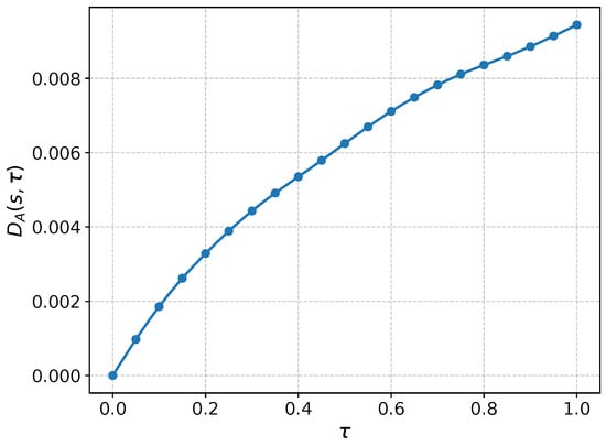
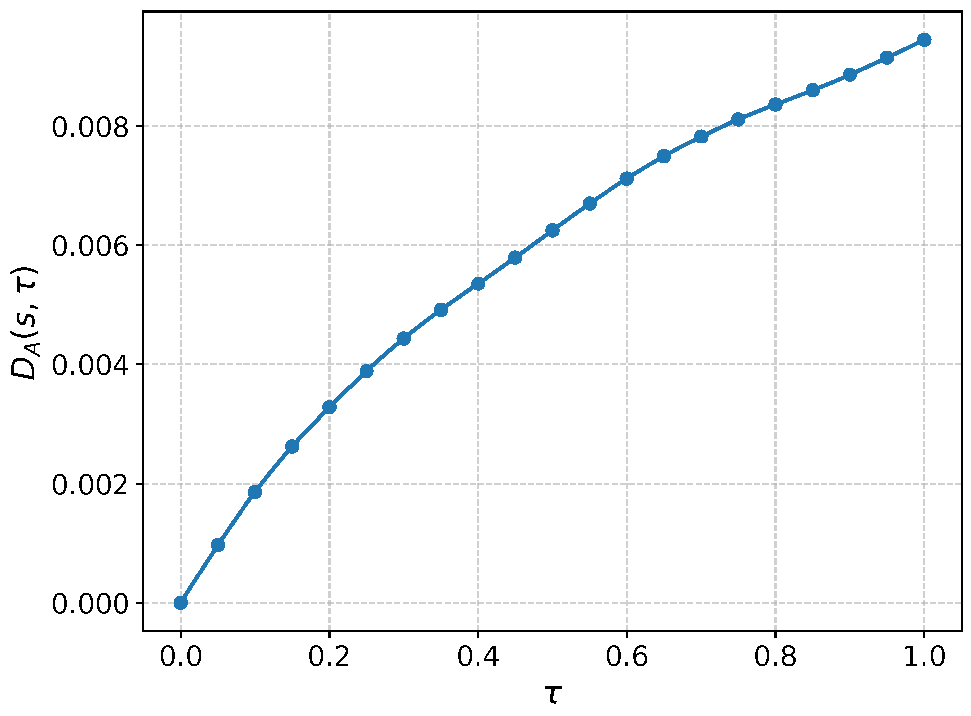
To quantify the evolution of the observable independently of its absolute scale, the normalized Frobenius distance is defined as

$$D_A(\mathbf{s},\tau )={\displaystyle \frac{\parallel A_{\mathrm{KL}}(\mathbf{s},\tau )-A_{\mathrm{KL}}{(\mathbf{s},0)\parallel }_F}{\parallel A_{\mathrm{KL}}{(\mathbf{s},0)\parallel }_F}}.$$

Figure 1 shows that the normalized distance increases from zero as $\tau$ evolves, confirming numerically that $A_{\mathrm{KL}}(\mathbf{s},\tau )\ne A_{\mathrm{KL}}(\mathbf{s},0)$. This result is consistent with the non-zero commutator obtained before.

Figure 1. Normalized evolution of the observable operator, $D_A(\mathbf{s},\tau )$, as a function of the Heisenberg evolution parameter $\tau$.

Although the observable evolves, its trace remains invariant under the unitary evolution. The trace was evaluated for all 101 values of $\tau$. The maximum relative trace error was found to be $e_{\mathrm{Tr}}^{\max }={\max }_{\tau }{\displaystyle \frac{|\mathrm{Tr}\left[A_{\mathrm{KL}}(\mathbf{s},\tau )\right]-\mathrm{Tr}\left[A_{\mathrm{KL}}(\mathbf{s},0)\right]|}{\left|\mathrm{Tr}\right[A_{\mathrm{KL}}(\mathbf{s},0)\left]\right|}}=3.60\times {10}^{-16}$. Numerically, this error is of the order of machine precision, confirming the conservation of the trace during the unitary evolution.

8.2. Example 2: ${\int }_{\mathsf{\Omega }}{\mathbb{E}\left[\right|U(\mathbf{s},t;\alpha )|}^2]d\mathbf{s}dt={\sum }_I{\lambda }_I=\mathrm{Tr}\left[C\right]$

The goal of this example is to show that the expected value of the square of a stochastic field expanded using the KL expansion can be expressed as the trace of the operator. Since a zero mean stochastic field is considered in this example, that is, $\overline{u}(\mathbf{s},t)=0$, the following relation holds: ${\int }_{\mathsf{\Omega }}{\mathbb{E}\left[\right|u(\mathbf{s},t;\alpha )|}^2]d\mathbf{s}dt={\sum }_i{\lambda }_i=\mathrm{Tr}\left[C\right]$, therefore, the total integrated variance of the stochastic field is given by the trace of the covariance operator. The field is expressed as

$$u(\mathbf{s},t;\alpha )={\displaystyle \sum _{i=1}^{\infty }}\sqrt{{\lambda }_i}{\varphi }_i(\mathbf{s},t){\xi }_i\left(\alpha \right),$$

where ${\xi }_i\left(\alpha \right)$ are independent random variables with mean zero and unit variance.

To perform the numerical demonstration, the Matérn covariance given by expression (5), is constructed using the parameters $\eta ={\eta }_t=1.5$ and ${\ell }_s={\ell }_t=0.2$ for the spatial and temporal components. For this numerical example, a one-dimensional spatial domain $D=[0,1]\subset \mathbb{R}$ and a temporal domain $I=[0,1]$ are considered. The spatial and temporal domains are each discretized using 10 points, resulting in a total of 100 space-time points. Although this grid is a coarse discretization, it is sufficient for the purpose of numerically illustrating the results.

Once the Matérn covariance is obtained, a spectral decomposition is performed to determine the eigenvalues and eigenfunctions. To approximate the continuous space-time integrals consistently, a trapezoidal quadrature is introduced over the discretized domain. For the uniform grids considered in this article, the corresponding quadrature weights are determined by the spatial and temporal increments $\Delta s$ and $\Delta t$. Let W denote the diagonal matrix containing these space-time quadrature weights. A symmetric discrete representation of the covariance operator consistent with this quadrature is defined as

$$C_W=W^{1/2}C{W}^{1/2}.$$

The symmetric matrix $C_W$ is then spectrally decomposed. The eigenvectors of $C_W$ are transformed through $W^{-1/2}$ to obtain the discrete KL eigenfunctions, which satisfy the weighted orthogonality condition ${\varphi }_i^{T}W{\varphi }_j={\delta }_{i,j}$.

The eigenvalues used in the discrete KL expansion are obtained from $C_W$ so that

$$\sum _i{\lambda }_i=\mathrm{Tr}\left(C_W\right),$$

which provides a quadrature-based discrete approximation of the continuous relation ${\int }_{\mathsf{\Omega }}{\mathbb{E}\left[\right|u(\mathbf{s},t;\alpha )|}^2]d\mathbf{s}dt=\mathrm{Tr}\left[C\right]$.

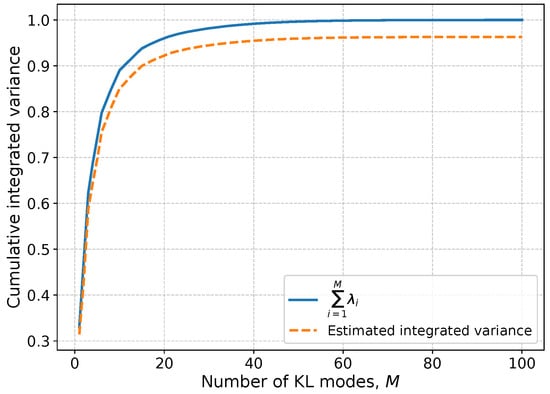
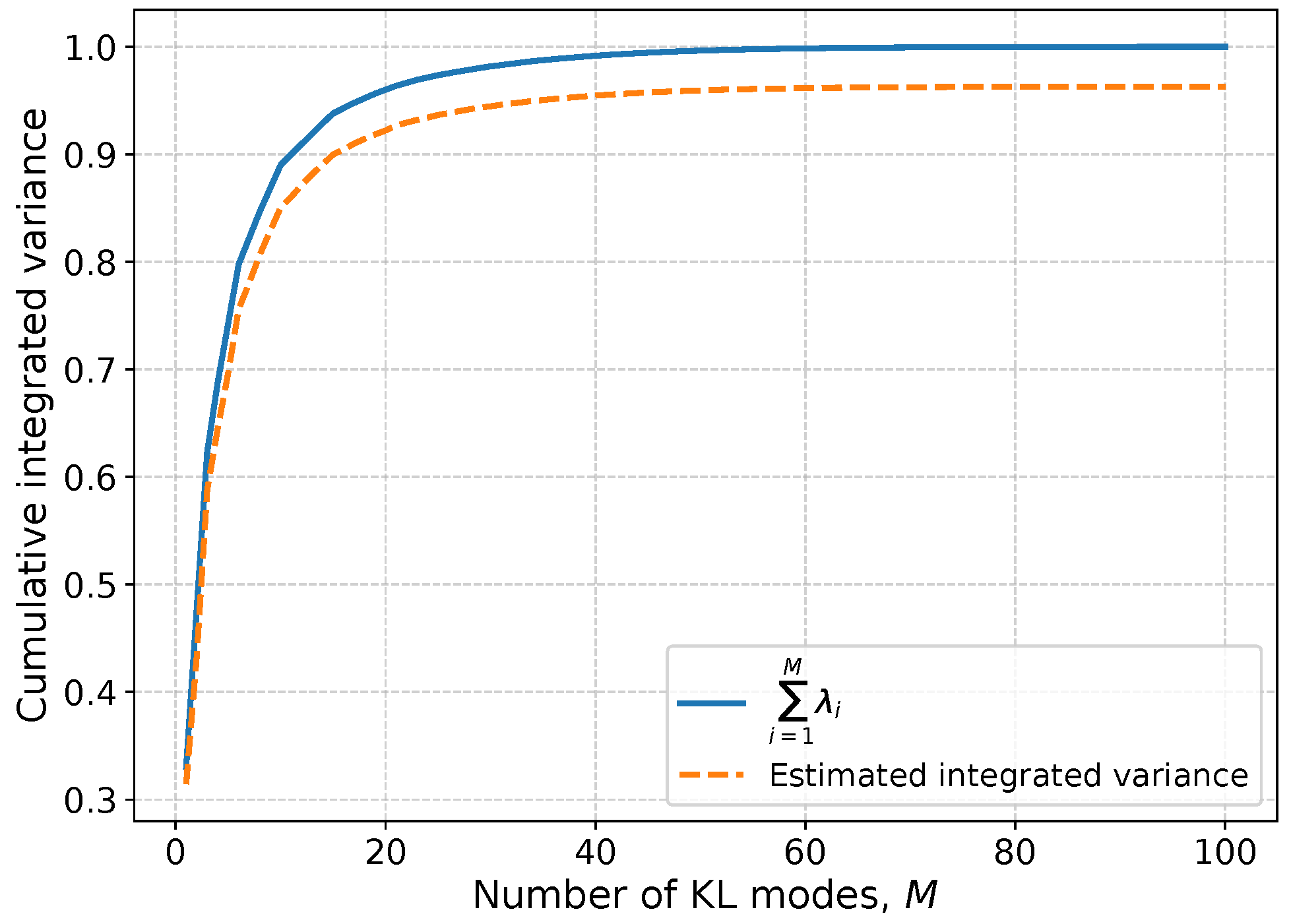
The KL discrete expansion with 100 modes is used, and 500 independent realizations are generated. The estimated integrated field variance, obtained from the 500 independent realizations and the trapezoidal quadrature, is ${\int }_{\mathsf{\Omega }}{\mathbb{E}\left[\right|u(\mathbf{s},t;\alpha )|}^2]d\mathbf{s}dt\approx 0.96301903$, while the sum of the eigenvalues is ${\sum }_i{\lambda }_i=1.00000000$. These two values differ by approximately $0.03698$ (a percentage difference of $3.70\%$), which is consistent with the finite number of stochastic realizations used to approximate the expectation.

Figure 2 compares the cumulative integrated field variance estimated from the stochastic realizations as a function of the number M of retained KL modes (dashed line) with the cumulative sum of the corresponding KL eigenvalues (solid line). As additional modes are incorporated, both quantities increase toward the total integrated variance.

Figure 2. Cumulative integrated field variance estimated with 500 independent stochastic realizations, and cumulative sum of KL eigenvalues, as functions of the number of retained KL modes M.

8.3. Example 3: Numerical Comparison with Standard and Hierarchical Bayesian Formulations

The purpose of this example is to verify numerically that the operator representation introduced in this work reproduces the Bayesian formulation when the initial observable $\widehat{A}(\mathbf{s},0)$ is identified, by assumption, with ${\mathsf{\Gamma }}_{\mathrm{noise}}^{-1}$, rather than to assess the performance of two independent Bayesian inference methods. Since the correspondence is established by representing the Bayesian quadratic form in the KL basis, agreement between the conventional and operator representations is expected when the complete basis is retained. These comparisons therefore serve to verify the numerical implementation of the correspondence established analytically in Theorem 1, at the levels of the quadratic form, posterior distributions and MAP estimates.

The comparison is performed at three levels: first, the Bayesian quadratic form is compared with its Heisenberg representation in the KL basis. Second, the complete posterior distribution and the corresponding maximum a posteriori (MAP) estimate are compared for a one parameter inverse problem. Finally, a hierarchical Bayesian benchmark is considered by introducing the observational noise amplitude as an additional unknown parameter.

As in the previous examples, the same space-time discretization and Matérn covariance are employed, with $N=100$ space-time points, a one dimensional spatial domain, ${\ell }_s={\ell }_t=0.2$ and $\eta ={\eta }_t=1.5$. The corresponding KL eigenvalues and eigenvectors are those obtained from the spectral decomposition introduced in Section 8.1. The observational noise covariance ${\mathsf{\Gamma }}_{\mathrm{noise}}$ is taken to be the same correlated and non-diagonal covariance introduced in Example 1 (Section 8.1), with $\sigma =0.05$, ${\delta }_s=0.15$ and ${\delta }_t=0.30$.

8.3.1. Quadratic Form Correspondence in the KL Basis

A synthetic field is defined as

$$\mathbf{f}\left(\mathit{\nu }\right)=\mathit{\nu }\sin \left(\pi \mathbf{s}\right)\cos \left(\pi t\right),$$

(49)

where $\mathit{\nu }$ is the scalar model parameter. Synthetic observations are generated from ${\mathit{\nu }}_{\mathrm{true}}=1$ by adding a realization of the correlated observational noise,

$${\mathbf{d}}^{obs}=\mathbf{f}\left({\mathit{\nu }}_{\mathrm{true}}\right)+\mathit{ϵ},\mathit{ϵ}\sim \mathcal{N}\left(\mathbf{0},{\mathsf{\Gamma }}_{\mathrm{noise}}\right).$$

For an arbitrary value $\mathit{\nu }$ of the model parameter, the residual is defined as

$$\mathbf{r}\left(\mathit{\nu }\right)={\mathbf{d}}^{obs}-\mathbf{f}\left(\mathit{\nu }\right).$$

Following the notation introduced in Appendix A, the residual can also be represented in the KL eigenfunction basis through the state

$$|{\mathsf{\Psi }}_r\left(\mathit{\nu }\right)⟩=\sum _i{r}_i\left(\mathit{\nu }\right)|{\varphi }_i⟩,$$

where $r_i\left(\mathit{\nu }\right)$ are the KL coefficients of the residual.

The quadratic form appearing in the standard Gaussian likelihood can be written as

$$J\left(\mathit{\nu }\right)=\mathbf{r}{\left(\mathit{\nu }\right)}^T{\mathsf{\Gamma }}_{\mathrm{noise}}^{-1}\mathbf{r}\left(\mathit{\nu }\right).$$

In the KL basis, the residual is represented as

$${\mathbf{r}}_{\mathrm{KL}}\left(\mathit{\nu }\right)={\varphi }^T\mathbf{r}\left(\mathit{\nu }\right),$$

while the initial observable is represented in the KL basis as

$$A_{\mathrm{KL}}(\mathbf{s},0)={\varphi }^T{\mathsf{\Gamma }}_{\mathrm{noise}}^{-1}\varphi .$$

The same Bayesian quadratic form expressed in KL basis is therefore

$$J_{\mathrm{KL}}\left(\mathit{\nu }\right)=⟨{\mathsf{\Psi }}_r\left(\mathit{\nu }\right)|\widehat{A}(\mathbf{s},0)|{\mathsf{\Psi }}_r\left(\mathit{\nu }\right)⟩={\mathbf{r}}_{\mathrm{KL}}^T\left(\mathit{\nu }\right)A_{\mathrm{KL}}(\mathbf{s},0){\mathbf{r}}_{\mathrm{KL}}\left(\mathit{\nu }\right).$$

To provide a non-trivial numerical comparison, an initial estimate of the unknown parameter $\mathit{\nu }=0.2$ is considered to evaluate the forward model and the corresponding residual. This estimate differs from the true value ${\mathit{\nu }}_{\mathrm{true}}=1$.

Using the complete KL basis, the numerical values obtained for a representative model given by the expression (49), are

$$J\left(\mathit{\nu }\right)=1358.2406213936108,$$

and

$$J_{\mathrm{KL}}\left(\mathit{\nu }\right)=1358.240621393612.$$

The corresponding relative error between $J\left(\mathit{\nu }\right)$ and $J_{\mathrm{KL}}\left(\mathit{\nu }\right)$ is $e_J={\displaystyle \frac{|J\left(\mathit{\nu }\right)-J_{\mathrm{KL}}\left(\mathit{\nu }\right)|}{\left|J\right(\mathit{\nu }\left)\right|}}=8.37\times {10}^{-16}$, showing that both representations agree up to numerical precision.

To investigate the effect of truncating the KL representation, the quadratic form is also evaluated using only the first M modes,

$$J_{\mathrm{KL}}^{\left(M\right)}\left(\mathit{\nu }\right)={\mathbf{r}}_M^T\left(\mathit{\nu }\right)A_M{\mathbf{r}}_M\left(\mathit{\nu }\right),$$

where

$${\mathbf{r}}_M\left(\mathit{\nu }\right)={\varphi }_M^T\mathbf{r}\left(\mathit{\nu }\right),A_M={\varphi }_M^T{\mathsf{\Gamma }}_{\mathrm{noise}}^{-1}{\varphi }_M.$$

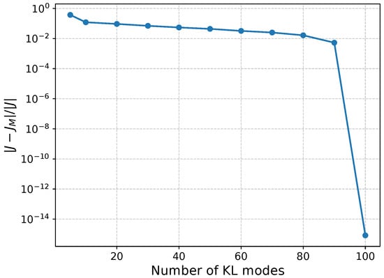
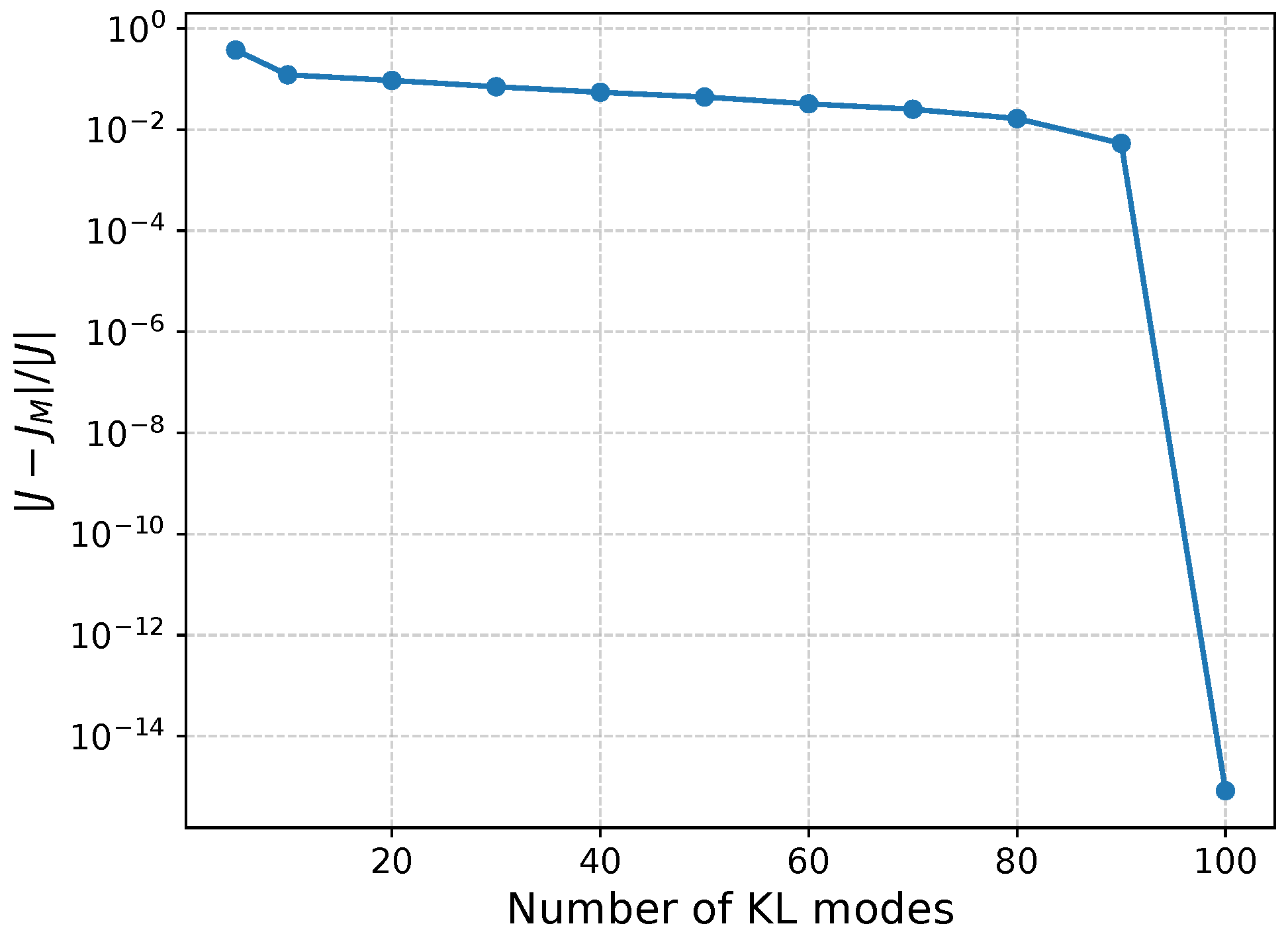
Figure 3 shows the relative discrepancy as the number of retained KL modes is increased, calculated by the expression $e_{\mathrm{rel}}^{\left(M\right)}={\displaystyle \frac{|J\left(\mathit{\nu }\right)-J_{\mathrm{KL}}^{\left(M\right)}\left(\mathit{\nu }\right)|}{\left|J\right(\mathit{\nu }\left)\right|}}$. It can be seen that the discrepancy decreases as additional modes are incorporated, and the complete representation $M=N=100$ recovers the standard quadratic form with a relative error of $8.37\times {10}^{-16}$.

Figure 3. Relative discrepancy between the standard Bayesian quadratic form and its truncated representation in the KL basis as a function of the number of retained KL modes.

8.3.2. Comparison of the Bayesian Posterior and MAP Estimate

The previous comparison verifies the quadratic form correspondence for a fixed value $\mathit{\nu }$. To verify that the correspondence also holds at the level of the complete Bayesian inverse problem, the parameter $\mathit{\nu }$ is treated as unknown and evaluated over the interval:

$$\mathit{\nu }\in [0.7,1.3].$$

A Gaussian prior is considered,

$$\mathit{\nu }\sim \mathcal{N}\left({\mathit{\nu }}_0,{\sigma }_{\mathit{\nu }}^2\right),$$

with

$${\mathit{\nu }}_0=1,{\sigma }_{\mathit{\nu }}=0.15.$$

Since the observational covariance is fixed in this comparison, the Bayesian likelihood is proportional to

$$\mathcal{L}\left({\mathbf{d}}^{obs}\right|\mathit{\nu })\propto \exp \left[-{\displaystyle \frac{1}{2}}\mathbf{r}{\left(\mathit{\nu }\right)}^T{\mathsf{\Gamma }}_{\mathrm{noise}}^{-1}\mathbf{r}\left(\mathit{\nu }\right)\right].$$

Using the Heisenberg representation expressed in the KL eigenfunction basis at $\tau =0$, the corresponding likelihood is

$${\mathcal{L}}^{\mathrm{KL}}({\mathbf{d}}^{obs}\mid \mathit{\nu })\propto \exp \left[-{\displaystyle \frac{1}{2}}⟨{\mathsf{\Psi }}_r\left(\mathit{\nu }\right)|\widehat{A}(\mathbf{s},0)|{\mathsf{\Psi }}_r\left(\mathit{\nu }\right)⟩\right].$$

Combining each likelihood with the same prior gives the corresponding posterior distributions

$$\begin{array}{cc}\hfill f_{\mathrm{post}}\left(\mathit{\nu }\right|{\mathbf{d}}^{obs})& \propto \mathcal{L}({\mathbf{d}}^{obs}\mid \mathit{\nu }){\mathcal{L}}_{\mathrm{prior}}\left(\mathit{\nu }\right)\hfill \end{array}$$

(50)

$$\begin{array}{cc}\hfill f_{post}^{\mathrm{KL}}\left(\mathit{\nu }\right|{\mathbf{d}}^{obs})& \propto {\mathcal{L}}^{\mathrm{KL}}({\mathbf{d}}^{obs}\mid \mathit{\nu }){\mathcal{L}}_{prior}\left(\mathit{\nu }\right).\hfill \end{array}$$

(51)

Over the complete parameter interval, the maximum relative discrepancy between the Bayesian quadratic form and its representation in the KL eigenfunction basis is

$$\underset{\mathit{\nu }}{\max }{\displaystyle \frac{\left|{\mathbf{r}}^T{\mathsf{\Gamma }}_{\mathrm{noise}}^{-1}\mathbf{r}-{\mathbf{r}}_{\mathrm{KL}}^T{A}_{\mathrm{KL}}(\mathbf{s},0){\mathbf{r}}_{\mathrm{KL}}\right|}{\left|{\mathbf{r}}^T{\mathsf{\Gamma }}_{\mathrm{noise}}^{-1}\mathbf{r}\right|}}=1.10\times {10}^{-15}.$$

The maximum absolute difference between the resulting posterior densities is

$$\underset{\mathit{\nu }}{\max }\left|f_{\mathrm{post}}\left(\mathit{\nu }\right|{\mathbf{d}}^{obs})-f_{\mathrm{post}}^{\mathrm{KL}}\left(\mathit{\nu }\right|{\mathbf{d}}^{obs})\right|=3.34\times {10}^{-13}.$$

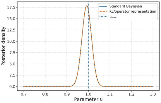
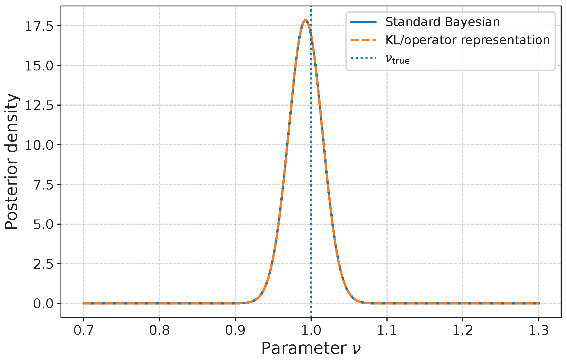
Figure 4 compares both posterior distributions. The two curves overlap within numerical precision.

Figure 4. Comparison between the posterior density obtained using the Bayesian formulation and the Heisenberg representation expressed in the KL eigenfunction basis at $\tau =0$. The vertical line indicates the true value ${\mathit{\nu }}_{\mathrm{true}}=1$.

Both formulations produce the same grid-based MAP estimate,

$${\mathit{\nu }}_{\mathrm{MAP}}={\mathit{\nu }}_{\mathrm{MAP}}^{\mathrm{KL}}=0.992.$$

The agreement between the two posterior distributions and their corresponding MAP estimates numerically confirms the equivalence between the standard and the Heisenberg representation expressed in the KL eigenfunction basis at $\tau =0$ for this example.

8.3.3. Hierarchical Bayesian Benchmark

As an additional benchmark, a hierarchical Bayesian formulation is considered in which the overall amplitude of the observational noise and the forward model parameter $\mathit{\nu }$ from Equation (49) are treated as unknown. Unlike the previous comparisons in Section 8.3.1 and Section 8.3.2, where the observational covariance is known, the covariance is now parameterized as

$${\mathsf{\Gamma }}_{\mathrm{noise}}\left(\sigma \right)={\sigma }^2{R}_{i,j},$$

where $R_{i,j}$ is the same fixed space-time correlation matrix introduced previously, and $\sigma >0$ controls the overall amplitude of the observational noise. In this case, the unknown parameters are $\mathit{\nu }$ and $\sigma$.

The synthetic observations used in this benchmark are generated using the true values: ${\mathit{\nu }}_{\mathrm{true}}=1$ and ${\sigma }_{\mathrm{true}}=0.05$. These values are used only to generate the synthetic observations and are treated as unknown during the hierarchical inference.

The unknown parameters are treated as a vector $\mathit{\theta }=[\mathit{\nu },\sigma ]$. Thus, the residual is written as $\mathbf{r}\left(\mathit{\theta }\right)={\mathbf{d}}^{\mathrm{obs}}-\mathbf{f}\left(\mathit{\nu }\right)$, and the quadratic form entering the Gaussian likelihood becomes

$${\mathbf{r}}^T\left(\mathit{\theta }\right){\mathsf{\Gamma }}_{\mathrm{noise}}^{-1}\left(\sigma \right)\mathbf{r}\left(\theta \right).$$

In the Heisenberg representation expressed in the KL eigenfunction basis at $\tau =0$, the corresponding quadratic form is

$$⟨{\mathsf{\Psi }}_r\left(\mathit{\theta }\right)|\widehat{A}(\mathbf{s},0;\sigma )|{\mathsf{\Psi }}_r\left(\mathit{\theta }\right)⟩={\mathbf{r}}_{\mathrm{KL}}^T\left(\mathit{\theta }\right)A_{\mathrm{KL}}(\mathbf{s},0;\sigma ){\mathbf{r}}_{\mathrm{KL}}\left(\mathit{\theta }\right),$$

with $|{\mathsf{\Psi }}_r\left(\mathit{\theta }\right)⟩=|{\mathsf{\Psi }}^{obs}⟩-|\mathsf{\Psi }\left(\mathit{\theta }\right)⟩$ and

$$A_{\mathrm{KL}}(\mathbf{s},0;\sigma )={\varphi }^T{\mathsf{\Gamma }}_{\mathrm{noise}}^{-1}\left(\sigma \right)\varphi .$$

Because the observational covariance depends on the unknown parameter $\sigma$, the logarithm of the likelihood, omitting terms that are constant with respect to $\mathit{\theta }$, is

$$\log \mathcal{L}({\mathbf{d}}^{\mathrm{obs}}\mid \mathit{\theta })=-{\displaystyle \frac{1}{2}}⟨{\mathsf{\Psi }}_r\left(\mathit{\theta }\right)|\widehat{A}(\mathbf{s},0;\sigma )|{\mathsf{\Psi }}_r\left(\mathit{\theta }\right)⟩-{\displaystyle \frac{1}{2}}\log \det {\mathsf{\Gamma }}_{\mathrm{noise}}\left(\sigma \right)$$

According to Bayes’ theorem in (32), the posterior distribution of the two unknown parameters is

$$f_{\mathrm{post}}\left(\mathit{\theta }\right)\propto \mathcal{L}({\mathit{d}}^{\mathit{obs}}\mid \mathit{\theta }){\mathcal{L}}_{\mathrm{prior}}\left(\mathit{\theta }\right).$$

Independent Gaussian priors are assigned to the two unknown parameters, with $\mathit{\nu }\sim \mathcal{N}(0,0.5^2)$ and $\sigma \sim \mathcal{N}(0.07,0.{03}^2)$. The parameter $\sigma$ is evaluated over the interval $[0.02,0.10]$, which contains the true value ${\sigma }_{\mathrm{true}}=0.05$.

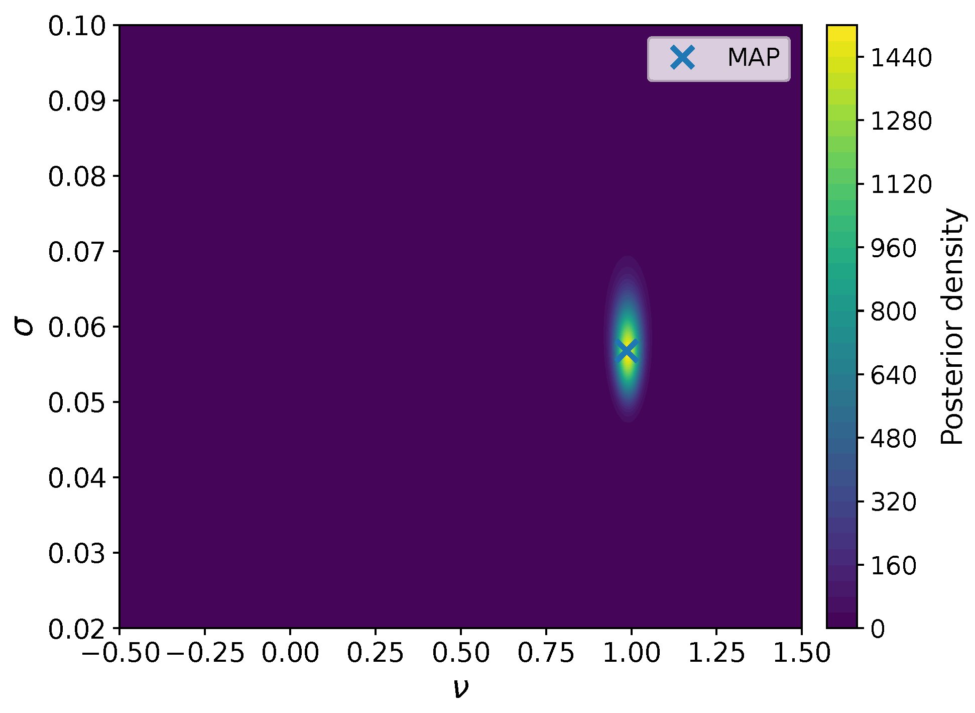
The hierarchical Bayesian formulation and the Heisenberg representation expressed in the KL eigenfunction basis produce the same MAP estimate,

$$({\mathit{\nu }}_{\mathrm{MAP}},{\sigma }_{\mathrm{MAP}})=(0.9867,0.0568).$$

The maximum relative discrepancy between the two Bayesian quadratic forms is $1.85\times {10}^{-15}$, while the maximum absolute difference between the resulting posterior densities is $5.28\times {10}^{-11}$.

Figure 5 shows the posterior density obtained in the hierarchical benchmark and the corresponding MAP location. The hierarchical Bayesian posterior and its posterior in the KL basis overlap within numerical precision. Therefore, only the standard hierarchical Bayesian posterior is shown.

Figure 5. Hierarchical posterior density in the parameter space $(\mathit{\nu },\sigma )$, obtained using the standard hierarchical Bayesian formulation. The marker indicates the MAP estimate $({\mathit{\nu }}_{\mathrm{MAP}},{\sigma }_{\mathrm{MAP}})=(0.9867,0.0568)$.

The hierarchical benchmark does not imply that the Heisenberg evolution parameter $\tau$ estimates the observational noise amplitude. The parameter $\sigma$ is estimated through the standard hierarchical Bayesian formulation, while the correspondence with the Heisenberg representation is evaluated at $\tau =0$ for each observational covariance considered.

9. Conclusions

This work establishes a formal correspondence between the Bayesian formulation of inverse problems and the Heisenberg representation. The central element of the proposed framework is the identification of the inverse observational noise covariance as the initial observable in the Heisenberg representation, according to the modeling hypothesis $\widehat{A}(\mathbf{s},0)\equiv {\mathsf{\Gamma }}_{\mathrm{noise}}^{-1}$.

The residual between the observational data and the forward model response is represented in the Karhunen–Loève basis obtained from a stochastic field with Matérn covariance. The same spectral structure is then used to construct the state and the Hamiltonian governing the Heisenberg evolution. Therefore, the Bayesian weighted quadratic form and the Heisenberg observable are expressed within the same operator framework.

The main theorem shows that, under the modeling hypothesis $\widehat{A}(\mathbf{s},0)\equiv {\mathsf{\Gamma }}_{\mathrm{noise}}^{-1}$, the quadratic form appearing in the Gaussian likelihood admits an equivalent representation in terms of the initial Heisenberg observable. The limiting cases of the Matérn covariance were also examined: when the correlation length tends to zero, the covariance vanishes between distinct points, whereas when the correlation length tends to infinity, the covariance tends to the field variance ${\sigma }_u^2$.

Three numerical examples were presented in Section 8. The first example considers a correlated, non-diagonal observational covariance and yields a non-zero commutator between the initial observable and the Hamiltonian $\left|\right|[A_{\mathrm{KL}}(\mathbf{s},0),H_{\mathrm{KL}}]{\left|\right|}_F=442.0143$, thereby producing a non-trivial Heisenberg evolution, while the trace remains invariant up to numerical precision. The second numerical example verifies the relation between the trace of the Matérn covariance operator and the integrated variance represented through the KL expansion using 500 independent realizations. The estimated integrated variance differs from the sum of the KL eigenvalues by approximately $3.70\%$. The third example confirms the equivalence between the Bayesian quadratic form and its operator representation in the KL basis. In Section 8.3.1, synthetic data were generated from a forward model $f\left(\mathit{\nu }\right)$ by adding correlated Gaussian noise. Using the complete KL basis, the relative discrepancy is approximately $8.37\times {10}^{-16}$, confirming the numerical equivalence between these two representations. The corresponding posterior distributions $f_{\mathrm{post}}$ and $f_{\mathrm{post}}^{\mathrm{KL}}$ also agree within numerical precision, with a maximum absolute difference of $3.34\times {10}^{-13}$. In both cases, the same MAP is obtained: ${\mathit{\nu }}_{\mathrm{MAP}}={\mathit{\nu }}_{\mathrm{MAP}}^{\mathrm{KL}}=0.992$. In addition, Section 8.3.3 compares the hierarchical benchmark with the Heisenberg representation expressed in the KL basis, where the model parameter $\mathit{\nu }$ and the observational noise amplitude $\sigma$ were treated as unknown parameters in the inverse problem. The numerical results yielded a maximum absolute difference equal to $5.28\times {10}^{-11}$ and the estimated parameter vector was $({\mathit{\nu }}_{\mathrm{MAP}},{\sigma }_{\mathrm{MAP}})=(0.9867,0.0568)$ in both formulations.

The numerical agreement between the conventional Bayesian formulation and its representation in the KL basis should not be interpreted as evidence of a new inference method. Rather, it confirms the consistency of the formal correspondence under the adopted modeling hypothesis. The distinctive feature of the proposed framework lies in representing the inverse observational noise covariance as the initial observable within the Heisenberg representation. Theorem 1 establishes the formal correspondence with the Bayesian likelihood at this initial observable, while the structural propositions in Section 7 describe properties of the operator framework, including unitary evolution and trace invariance. The evolution of the observable is illustrated numerically in Section 8.1 and does not modify the Bayesian inference procedure considered here. This correspondence does not imply a physical quantization of the underlying inverse problem. Possible extensions of this work include more general nonlinear forward models and formulations in which the inverse observational noise covariance is only partially known or must be characterized within the operator framework. Future work may also investigate the numerical properties of the proposed operator representation, convergence and computational performance under different numerical implementations.

References

- Abugattas, C.; Carpio, A.; Cebrián, E. Uncertainty quantification in inverse scattering problems. Entropy 2026, 28, 461. [Google Scholar] [CrossRef] [Scilit] [PubMed]
- Aster, R.C.; Borchers, B.; Thurber, C.H. Parameter Estimation and Inverse Problems, 3rd ed.; Elsevier: Amsterdam, The Netherlands, 2018. [Google Scholar]
- Carpio, A.; Cebrián, E.; Gutiérrez, A. Object based Bayesian full-waveform inversion for shear elastography. Inverse Probl. 2023, 39, 075007. [Google Scholar] [CrossRef] [Scilit]
- Kaipio, J.; Somersalo, E. Statistical and Computational Inverse Problems; Springer: New York, NY, USA, 2005. [Google Scholar]
- Carpio, A.; Iakunin, S.; Stadler, G. Bayesian approach to inverse scattering with topological priors. Inverse Probl. 2020, 36, 105001. [Google Scholar] [CrossRef] [Scilit]
- Levenberg, K. A method for the solution of certain non-linear problems in least squares. Q. Appl. Math. 1944, 2, 164–168. [Google Scholar] [CrossRef] [Scilit]
- Marquardt, D.W. An algorithm for least-squares estimation of nonlinear parameters. J. Soc. Ind. Appl. Math. 1963, 11, 431–441. [Google Scholar] [CrossRef] [Scilit]
- Tarantola, A. Inverse Problem Theory and Methods for Model Parameter Estimation; SIAM: Philadelphia, PA, USA, 2005. [Google Scholar]
- Stuart, A.M. Inverse problems: A Bayesian perspective. Acta Numer. 2010, 19, 451–559. [Google Scholar] [CrossRef] [Scilit]
- Nakahara, M. Geometry, Topology and Physics, 2nd ed.; CRC Press: Boca Raton, FL, USA, 2003. [Google Scholar]
- Cvetković, N.; Lie, H.C.; Bansal, H.; Veroy, K. Choosing Observation Operators to Mitigate Model Error in Bayesian Inverse Problems. SIAM/ASA J. Uncertain. Quantif. 2024, 12, 723–758. [Google Scholar] [CrossRef] [Scilit]
- Mathé, P. Bayesian inverse problems with non-commuting operators. Math. Comput. 2019, 88, 2897–2912. [Google Scholar] [CrossRef] [Scilit]
- Reed, M.; Simon, B. Methods of Modern Mathematical Physics I: Functional Analysis, 2nd ed.; Academic Press: New York, NY, USA, 1980. [Google Scholar]
- Ghanem, R.G.; Spanos, P.D. Stochastic Finite Elements: A Spectral Approach; Dover Publications: Mineola, NY, USA, 2003. [Google Scholar]
- Sakurai, J.J.; Napolitano, J. Modern Quantum Mechanics, 3rd ed.; Cambridge University Press: Cambridge, UK, 2020. [Google Scholar]
- Dereziński, J. Mathematical Introduction to Quantum Field Theory; Department of Mathematical Methods in Physics, University of Warsaw: Warsaw, Poland, 2020. [Google Scholar]
- Fetter, A.L.; Walecka, J.D. Quantum Theory of Many-Particle Systems; Dover Publications: Mineola, NY, USA, 2003. [Google Scholar]
- Peskin, M.E.; Schroeder, D.V. An Introduction to Quantum Field Theory; Westview Press: Boulder, CO, USA, 1995. [Google Scholar]
- Attal, S. Fock Spaces; Lecture Notes; Institut Camille Jordan, Université Lyon 1: Lyon, France, 2015. [Google Scholar]
- Lindgren, F.; Rue, H.; Lindström, J. An explicit link between Gaussian fields and Gaussian Markov random fields: The stochastic partial differential equation approach. J. R. Stat. Soc. Ser. B Stat. Methodol. 2011, 73, 423–498. [Google Scholar] [CrossRef] [Scilit]
- Rue, H.; Held, L. Gaussian Markov Random Fields: Theory and Applications; Chapman & Hall/CRC: Boca Raton, FL, USA, 2005. [Google Scholar]
- Salcedo, L.L. Introducción a la Teoría de Campos Cuánticos; Lecture Notes; Departamento de Física Atómica, Molecular y Nuclear, Universidad de Granada: Granada, Spain, 2018. [Google Scholar]
- Momeni, D. Reconstructing configurational Hamiltonians from Fock space. Nucl. Phys. B 2025, 1019, 117119. [Google Scholar] [CrossRef] [Scilit]
- Janson, S. On distance covariance in metric and Hilbert spaces. ALEA Lat. Am. J. Probab. Math. Stat. 2021, 18, 1353–1393. [Google Scholar] [CrossRef] [Scilit]
- Abugattas, C.; Carpio, A.; Cebrián, E.; Oleaga, G. Quantifying uncertainty in inverse scattering problems set in layered environments. Appl. Math. Comput. 2025, 500, 129453. [Google Scholar] [CrossRef] [Scilit]
- Bishop, C.M. Pattern Recognition and Machine Learning; Springer: New York, NY, USA, 2006. [Google Scholar]
- Jaynes, E.T. Probability Theory: The Logic of Science; Cambridge University Press: Cambridge, UK, 2003. [Google Scholar]
- Horn, R.A.; Johnson, C.R. Matrix Analysis, 2nd ed.; Cambridge University Press: Cambridge, UK, 2013. [Google Scholar]
- Abramowitz, M.; Stegun, I.A. Handbook of Mathematical Functions; Dover Publications: New York, NY, USA, 1972. [Google Scholar]
Disclaimer/Publisher’s Note: The statements, opinions and data contained in all publications are solely those of the individual author(s) and contributor(s) and not of MDPI and/or the editor(s). MDPI and/or the editor(s) disclaim responsibility for any injury to people or property resulting from any ideas, methods, instructions or products referred to in the content. |
© 2026 by the author. Licensee MDPI, Basel, Switzerland. This article is an open access article distributed under the terms and conditions of the Creative Commons Attribution (CC BY) license.