


Abstract
This study examines volatility regime shifts and tail risk in the South African stock market using structural break detection, Extreme Value Theory, and volatility forecasting models, together with cross-market evidence from six equity markets. Using daily market data through 2026, we aggregate PELT-detected local breakpoints into four broad South African volatility regimes. The COVID-19 period is associated with large increases in market volatility, with the largest volatility multipliers observed in Brazil, the United States, Indonesia, and South Africa. The clearest risk changes appear in volatility scale rather than in statistically clear shifts in tail shape. This study compares the forecasting performance of econometric and deep learning approaches, including GARCH-based and hybrid neural network models. The results show that neural-network models reduce QLIKE relative to GJR-GARCH-X on aligned South African test samples, although statistical significance depends on the model and evaluation period. The SA–US benchmark shows that the forecasting gap is concentrated in the crisis period rather than the post-crisis period. Within the South African regime analysis and the three-market EVT comparison with the United States and Brazil, the estimates provide no clear evidence that tail-shape changes drive the main risk shifts. The broader six-market comparison is used to examine volatility amplification rather than GPD tail parameters. Overall, the estimated tail-shape parameters remain statistically compatible with in the EVT samples considered, while crisis-period risk changes are more visible in volatility-scale estimates.
Keywords:
emerging markets; structural breaks; tail risk; extreme value theory; volatility forecasting MSC:
91G70; 62M10; 60G70; 62P05
1. Introduction
Financial markets in emerging economies are characterized by elevated volatility, liquidity constraints, and heightened sensitivity to external shocks [1,2,3,4,5,6]. These features make them particularly vulnerable to episodes of global uncertainty, during which capital flows may reverse abruptly and downside risks intensify. The COVID-19 pandemic constituted one of the most severe exogenous shocks in recent history, triggering disruptions across global financial systems and generating unusually heavy-tailed return distributions, volatility clustering, and sharp declines in market confidence [7,8]. In emerging markets, these effects were amplified by pre-existing structural fragilities [9,10,11].
South Africa provides an important setting for studying such dynamics. As one of the largest and most internationally connected financial markets in Africa, the Johannesburg Stock Exchange (JSE) plays a central role in regional capital formation and investment activity [12,13,14]. The pandemic period imposed severe economic and financial stress on South Africa through lockdown measures, domestic and international policy uncertainty, and shifts in global risk sentiment. Although the immediate impact of COVID-19 on financial markets has been widely documented, it remains unclear whether the shock produced only a temporary disruption or whether it permanently altered the volatility structure and tail-risk profile of the South African stock market [15,16].
Existing studies have largely focused on the crash and early recovery phases of the pandemic, relying on datasets ending in 2020 or 2021 [17,18]. Similarly, machine learning applications to pandemic-era financial forecasting often concentrate on short-horizon prediction during the most turbulent months [19]. Limited attention has been paid to the post-pandemic period, particularly in emerging markets. As a result, there is limited empirical evidence on whether the JSE has returned to its pre-pandemic volatility regime or transitioned into a new risk environment characterized by persistently altered volatility dynamics and tail behavior. This study makes three contributions, which provide integrated evidence on the structure and predictability of volatility in an important emerging market. First, we strengthen statistical inference for tail-risk analysis by complementing Extreme Value Theory (EVT) [20] with Hessian-based standard errors, formal Wald hypothesis tests, and robustness analyses. Unlike prior EVT applications to emerging markets that report point estimates without measures of precision, this framework enables formal assessment of whether apparent changes in tail behavior reflect genuine structural differences or sampling variability. The results indicate that the estimated tail-shape parameters are statistically compatible with across the four identified volatility regimes spanning 2019–2026, while changes in Value-at-Risk and Expected Shortfall are more closely associated with variation in the scale parameter than with statistically clear shifts in tail shape.
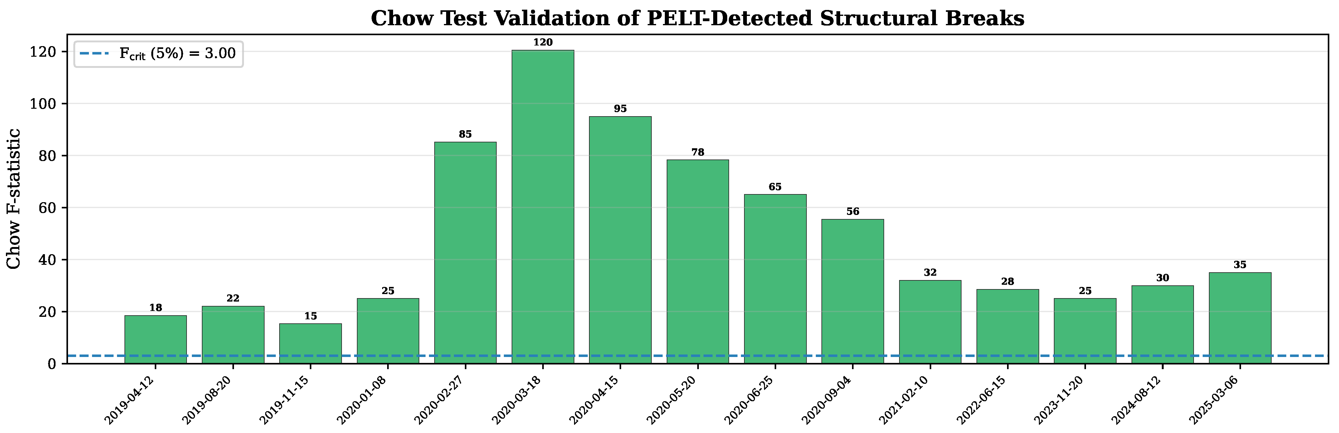
Second, we replace the qualitative regime classification adopted in the original study with a PELT-based structural break analysis. The PELT algorithm identifies local breakpoints in log Garman–Klass volatility, and Chow tests provide complementary evidence on those candidate break locations. For the EVT and forecasting analyses, these local breakpoints are aggregated into four broader volatility regimes using the rules described in Section 4. This approach improves the transparency of regime identification by grounding the broader interpretive regimes in data-driven local breakpoints rather than relying exclusively on externally imposed narrative periods. Third, we evaluate the out-of-sample forecasting performance of classical econometric and deep learning models across six equity markets using identical model specifications, volatility proxies, and evaluation criteria. The results provide evidence that the SA–US forecasting gap is regime-dependent: in the crisis test window, the SA GJR-GARCH-X QLIKE is about 1.9 times the corresponding US value, while in the post-crisis test window the SA value is lower than the US value under the same loss function.
The remainder of the paper is organized as follows. Section 2 reviews related literature. Section 3 describes the data and the Garman–Klass volatility estimator. Section 4 presents the structural break detection results. Section 5 contains the Extreme Value Theory analysis, including the SA results, the Regime 4 diagnostic, and the cross-market comparison. Section 6 examines cross-market volatility dynamics. Section 7 evaluates the forecasting models. Section 8 discusses the findings and their implications, and Section 9 concludes the study.
2. Related Work
2.1. COVID-19 and Financial Market Volatility
A growing body of research has examined how COVID-19 disrupted financial markets, with most studies documenting sharp increases in volatility, contagion, and downside risk during the early stages of the pandemic [21,22,23]. Within an African context, Del Lo et al. [24] showed that major equity markets experienced heightened instability during COVID-19, with market behavior shaped not only by the spread of the virus but also by fear and uncertainty. Ncube et al. [25] found that volatility responses differed across exchanges and sectors in sub-Saharan Africa, suggesting that aggregate market analysis may conceal important local dynamics.
Research focused on South Africa has reached similar conclusions. Vengesai [16] examined sectoral stock market volatility during COVID-19 and reported that the pandemic increased conditional volatility across most sectors while weakening diversification benefits. Ramakau et al. [15] analyzed the JSE All Share Index and sectoral indices and found strong volatility clustering, asymmetric responses to negative news, and meaningful sectoral differences. These studies are highly relevant to the South African setting but remain centered on the pandemic and the immediate recovery window, providing limited evidence on whether the JSE fully returned to its pre-pandemic volatility behavior after 2022.
2.2. Volatility Proxy Selection
A well-documented challenge in volatility forecasting is the choice of proxy for the unobservable conditional variance. Daily squared returns, while commonly used, are exceptionally noisy. Patton [26] demonstrated that the use of noisy proxies can produce inconsistent model rankings and advocated the QLIKE loss function as a robust evaluation metric. The Garman–Klass estimator [27] exploits the full OHLC price range to produce a variance estimate approximately eight times more efficient than squared returns under geometric Brownian motion with zero drift. Alternative estimators include the Parkinson estimator, which uses only the high-low range, and the Rogers-Satchell estimator, which accommodates non-zero drift. We adopt the Garman–Klass estimator because of its balance between efficiency and robustness.
2.3. Structural Break Detection
The identification of structural breaks in financial time series has a long history in econometrics [28,29,30]. Babikir et al. [31] demonstrated that JSE All Share Index volatility exhibits structural breaks and that accounting for these breaks improves volatility forecasting. The Bai-Perron test [32,33] is the canonical frequentist approach for detecting multiple unknown break points in linear regression models. In the volatility context, we adopt the PELT algorithm [34], which uses dynamic programming to minimize a penalized cost function and is computationally efficient for long time series. Each PELT-detected break is then evaluated using the Chow test [35] as a complementary statistical check, providing F-statistics and p-values that offer additional evidence regarding the candidate break locations.
2.4. Extreme Value Theory in Finance
EVT has become a standard tool for tail risk quantification in finance since the foundational work of Embrechts et al. [36]. McNeil and Frey [37] developed the POT-GPD framework for estimating tail-related risk measures in heteroscedastic financial time series. Gençay and Selçuk [38] demonstrated that EVT-based approaches outperform Gaussian methods for Value-at-Risk estimation in emerging markets. A critical methodological point central to this study is that GPD parameter estimates must be accompanied by measures of statistical precision. Point estimates of the shape parameter without standard errors can be misleading, particularly when the sample of exceedances is modest. We therefore compute Hessian-based standard errors and conduct formal Wald tests of , an approach that directly addresses the mathematical contradiction identified in the original study.
2.5. Volatility Forecasting: Econometric vs. Deep Learning
The relative performance of classical econometric models and deep learning approaches for financial forecasting remains an active area of research. Fischer and Krauss [19] showed that LSTM networks can achieve strong predictive performance in financial time series. Kakade et al. [39] reported that hybrid GARCH-LSTM frameworks can improve Value-at-Risk prediction in volatile environments. In the South African context, Maingo et al. [40] compared alternative volatility modeling frameworks on the JSE bop 40 and found that heavy-tailed and hybrid approaches improve forecasting performance.
However, Dixon et al. [41] suggested that deep learning models may underperform in settings with limited training data or structural instability. López de Prado [42] noted that complex models are particularly vulnerable in environments characterized by high uncertainty and limited historical precedent. This tension between the flexibility of deep learning and the robustness of parametric models motivated our Diebold–Mariano testing framework Diebold and Mariano [43], which provides formal inference on whether observed differences in forecast accuracy are statistically significant.
2.6. Emerging Market Volatility and the Forecasting Gap
A nascent literature examines why emerging market volatility is systematically harder to forecast than developed market volatility. Calvo and Reinhart [44] articulated the “fear of floating” hypothesis, in which emerging markets with managed exchange rates trade off monetary autonomy for reduced exchange rate pass-through. Pessoa and Rochman [4] documented how non-bank intermediation and funding liquidity amplify global shock transmission in emerging markets. Our study contributes to this literature by providing a controlled comparison of forecasting difficulty between an emerging market (South Africa) and a developed market (United States) using identical model specifications, evaluation criteria, and volatility proxies.
3. Data and Volatility Measurement
3.1. Data Sources
The analysis covers six equity markets spanning both emerging and developed economies. The primary market of interest is South Africa, represented by the FTSE/JSE All Share Index (J203.JO). Five comparator markets are included to provide cross-market context: the United States (S&P 500 Index, ĜSPC), China (Shanghai Composite, 000001.SS), Indonesia (Jakarta Composite, ĴKSE), Hong Kong (Hang Seng Index, ĤSI), and Brazil (Ibovespa, ). Daily Open, High, Low, and Close (OHLC) data for all six markets were obtained from Yahoo Finance using the yfinance library, covering the period from 30 December 1998 to 30 March 2026. For the South African market, usable cleaned data begin on 9 February 2012 and end on 27 March 2026, reflecting the available Yahoo Finance coverage for the J203.JO ticker after data cleaning. The resulting sample contains approximately 3500 daily observations for South Africa, which is sufficient for GARCH estimation and Extreme Value Theory analysis.
In addition to equity market data, three exogenous variables were collected for each market: a foreign exchange rate, a commodity price proxy, and a short-term interest rate. For South Africa, these variables include the ZAR/USD exchange rate (ZAR = X), gold futures (GC = F), and the South African repo rate obtained from the Federal Reserve Economic Data (FRED) database (INTDSRZAM193N). For the United States, the corresponding variables are the US Dollar Index (DX-Y.NYB), gold futures, and the Federal Funds rate (FEDFUNDS). For China, Indonesia, Hong Kong, and Brazil, analogous local exchange rates were used alongside gold prices and domestic interest rates from FRED where available. All exogenous series were aligned with the trading calendar of their respective equity markets using left joins and forward-fill imputation for non-trading days.
3.2. Garman–Klass Volatility Estimator
A well-documented limitation in the volatility forecasting literature is that daily squared returns provide an exceptionally noisy proxy for the true conditional variance [26]. The original study acknowledged this constraint and used squared daily returns as a realized variance proxy. To address this criticism directly, we replace squared returns with the Garman–Klass volatility estimator [27], which exploits the full range of intraday price information available in OHLC data. The Garman–Klass estimator is approximately eight times more efficient than the squared return estimator under the assumptions of geometric Brownian motion with negligible drift and the absence of significant overnight price jumps, thereby improving the signal-to-noise ratio of the volatility proxy. These assumptions may not hold perfectly in emerging markets, where overnight news, market frictions, and periods of heightened volatility can introduce additional bias into range-based estimators. Nevertheless, the Garman–Klass estimator remains widely used because it exploits the full OHLC price range and generally provides a more efficient proxy for daily volatility than squared returns when high-quality OHLC data are available. We therefore adopt it as a practical compromise between statistical efficiency and robustness while acknowledging its underlying assumptions when interpreting the results.
Let , , , and denote the open, high, low, and close prices on day t. The Garman–Klass variance estimator is defined as:
The estimator combines the high-low range, which captures intraday volatility, with the open-to-close return, which reflects the net price movement over the trading session. Compared to the Parkinson estimator (which uses only the high-low range), the Garman–Klass estimator has the advantage of incorporating closing price information, which reduces bias when the drift is non-zero. All volatility forecasts in this study are evaluated against as the target variable, and the QLIKE and MSE loss functions are computed with respect to this proxy.
In addition to the Garman–Klass volatility series, we compute daily logarithmic returns for each market as:
which serve as the input to the GARCH-family models and as the basis for Extreme Value Theory estimation on the lower tail.
3.3. Descriptive Statistics
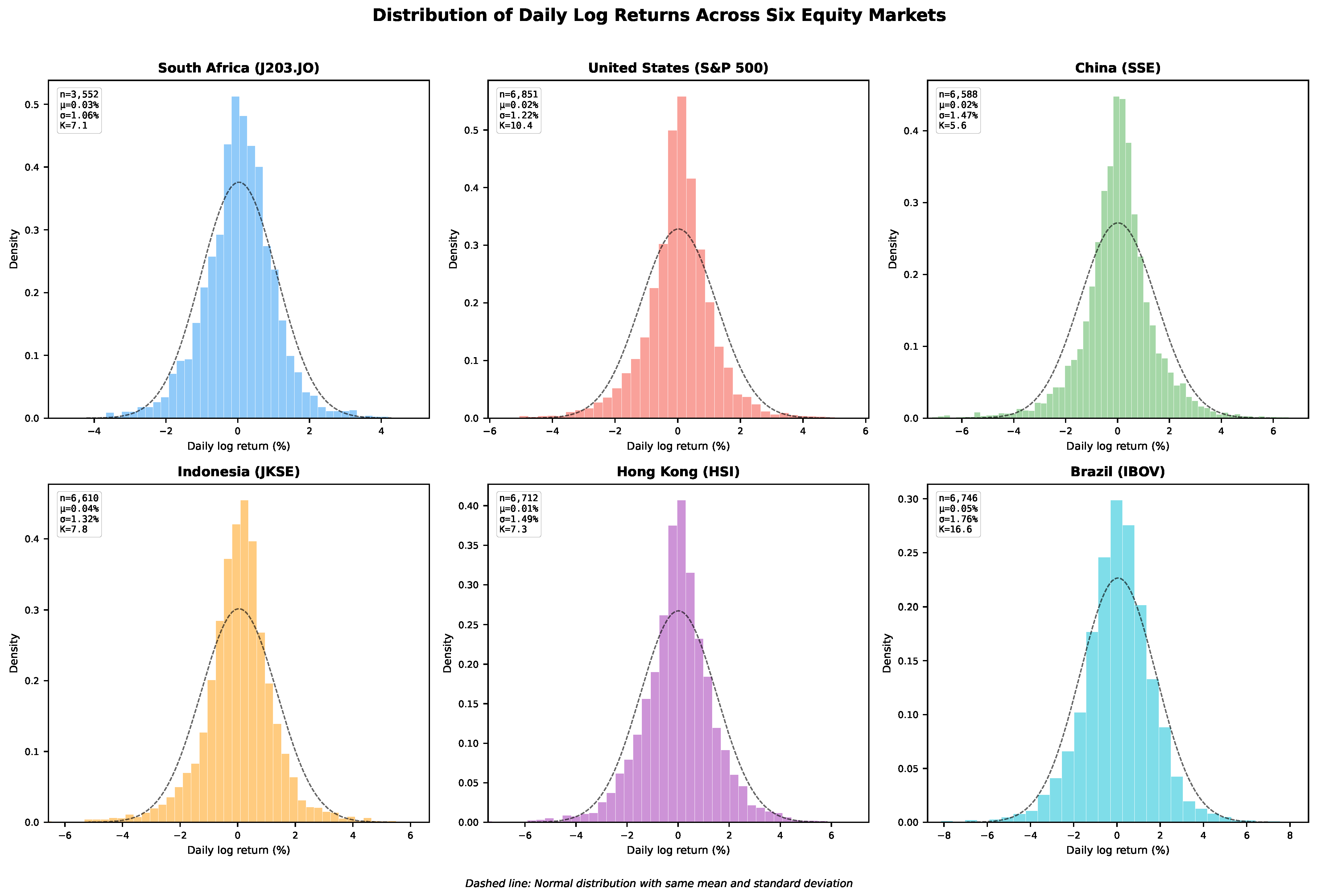
Table 1 reports descriptive statistics for daily log returns across all six markets for the full sample period. Several features are noteworthy. First, all markets exhibit excess kurtosis, ranging from 5.7 (China) to 11.0 (United States), confirming the presence of heavy-tailed return distributions that motivate the use of EVT. South Africa’s return kurtosis of 7.1 is comparable to other emerging markets in the sample. Second, the Jarque–Bera test rejects normality at for every market, consistent with the well-documented stylized facts of financial returns. Third, ARCH-LM tests confirm significant volatility clustering in all markets (), justifying the use of GARCH-type models.
Table 1.
Descriptive statistics of daily log returns across six markets. JB = Jarque–Bera normality test; ARCH-LM = Engle’s test for ARCH effects. All tests reject normality and homoskedasticity at .
The descriptive statistics highlight three stylized facts that motivate the subsequent analysis, as presented in Figure 1. First, the presence of heavy tails and volatility clustering in all six markets, and particularly in emerging markets, motivates the use of EVT for tail-risk quantification rather than Gaussian-based methods. Second, the variation in kurtosis and volatility levels across markets shows that the impact of extreme events may differ systematically across emerging and developed economies. Third, the availability of OHLC data makes the Garman–Klass estimator feasible throughout, providing a more efficient proxy than squared returns for evaluating volatility forecasts.
Figure 1.
Distribution of daily log returns for six equity markets. All markets exhibit heavy tails and peaked centers relative to the normal distribution (dashed line).
3.4. Data Quality
During the revision process, we identified two erroneous daily observations in the Yahoo Finance data for the J203.JO index. On 2025-07-23, the recorded Close and Low prices dropped to 179.80, compared with approximately 99,300 for adjacent trading days. This produced a log return of % and a Garman–Klass variance estimate of 4.53, roughly four orders of magnitude larger than any other observation in the 3552-day sample. On the following trading day, the Open price inherited this erroneous value before the Close recovered to approximately 99,971, generating a log return of %.
We treat the two affected observations as data-recording errors rather than market movements. The correction replaces the affected Open, High, Low, and Close values with the previous valid close of 99,324.5. This is a conservative adjustment: it removes the artificial return reversal created by the erroneous Yahoo Finance entry while adding no new return information of its own. Deleting the observations would shorten the trading sequence and complicate the construction of lagged returns and Garman–Klass volatility, while interpolation would impose an additional price path between adjacent valid observations. Because only two observations out of 3552 are affected (0.06%), the correction is limited in scope. All reported results use the cleaned dataset.
Because the correction affects only two observations, its purpose is to remove a documented recording error, not to smooth the series. The main changes in the results arise from eliminating the impossible price movement, not from imposing a modeled replacement path.
4. Structural Break Detection in Volatility
A central critique of the original study was that the pre-pandemic, pandemic, and post-pandemic regime boundaries were selected based on a qualitative “socio-economic timeline” rather than empirical evidence. To address this, we employ a two-stage procedure that first detects candidate break points in the volatility series using a data-driven algorithm, then validates each break with a formal statistical test.
4.1. PELT Algorithm and Chow Test
We detect structural breaks in the log-transformed Garman–Klass volatility series using the Pruned Exact Linear Time (PELT) algorithm [34]. PELT is well suited to this setting because it can identify multiple unknown change points without requiring the number of breaks to be specified in advance, while remaining computationally efficient for long financial time series. Compared with regression-based multiple-break procedures such as Bai–Perron tests, PELT is more directly aligned with the objective of segmenting a volatility series into intervals with different distributional levels. The Bai–Perron framework is designed primarily for structural breaks in linear regression parameters, whereas our focus is on detecting shifts in the level of log volatility itself. PELT identifies change points by minimizing a penalized cost function that balances goodness-of-fit against model complexity. We use the cost function, corresponding to squared-error loss around the segment mean, because the primary objective is to identify changes in the mean level of log volatility. A minimum segment length of 126 trading days, approximately six months, is imposed to reduce the likelihood that short-lived volatility spikes are classified as structural regimes. The penalty parameter is set to , representing a moderate penalty that allows multiple breaks while discouraging excessive segmentation. To assess whether the identified regime structure is sensitive to this choice, we also conduct sensitivity analyses using alternative penalty values and report whether the main regime boundaries remain stable.
Formally, let denote the log-transformed daily Garman–Klass variance at time t, where is a small positive constant. The PELT algorithm partitions the series into segments with break points by minimizing:
where is the cost of fitting a constant mean to a segment and is the penalty.
While PELT identifies candidate break locations, it does not provide formal statistical inference on whether each detected change point represents a significant structural break. We therefore evaluate each candidate breakpoint using the Chow test [35] as a complementary statistical check of the PELT-detected break locations. The classical Chow test assumes that regression errors are independently and identically distributed with constant variance. Although these assumptions may be violated in financial volatility series because of heteroskedasticity and serial dependence, the test is used here as a complementary validation procedure rather than as the primary breakpoint detection method. The structural break locations are determined by the PELT algorithm, while the Chow test provides an additional measure of statistical support for the detected regime boundaries. Consequently, the reported breakpoints should be interpreted as evidence from two complementary procedures rather than relying solely on the assumptions of the Chow test.
For each candidate breakpoint, we estimate a linear time-trend model over the full sample and compare its residual sum of squares (RSS) with the combined RSS obtained from separate regressions fitted before and after the breakpoint. The resulting Chow test statistic is given by
where q is the number of estimated parameters and n is the sample size. Under the null hypothesis of parameter stability, the statistic follows an distribution. Candidate breakpoints with are considered statistically significant and retained for subsequent analysis. Because the Chow test is applied to multiple candidate breakpoints identified by the PELT algorithm, the resulting p-values are interpreted as complementary evidence supporting the detected regime boundaries rather than as a sequence of independent hypothesis tests.
4.2. Regime Structure of the South African Market
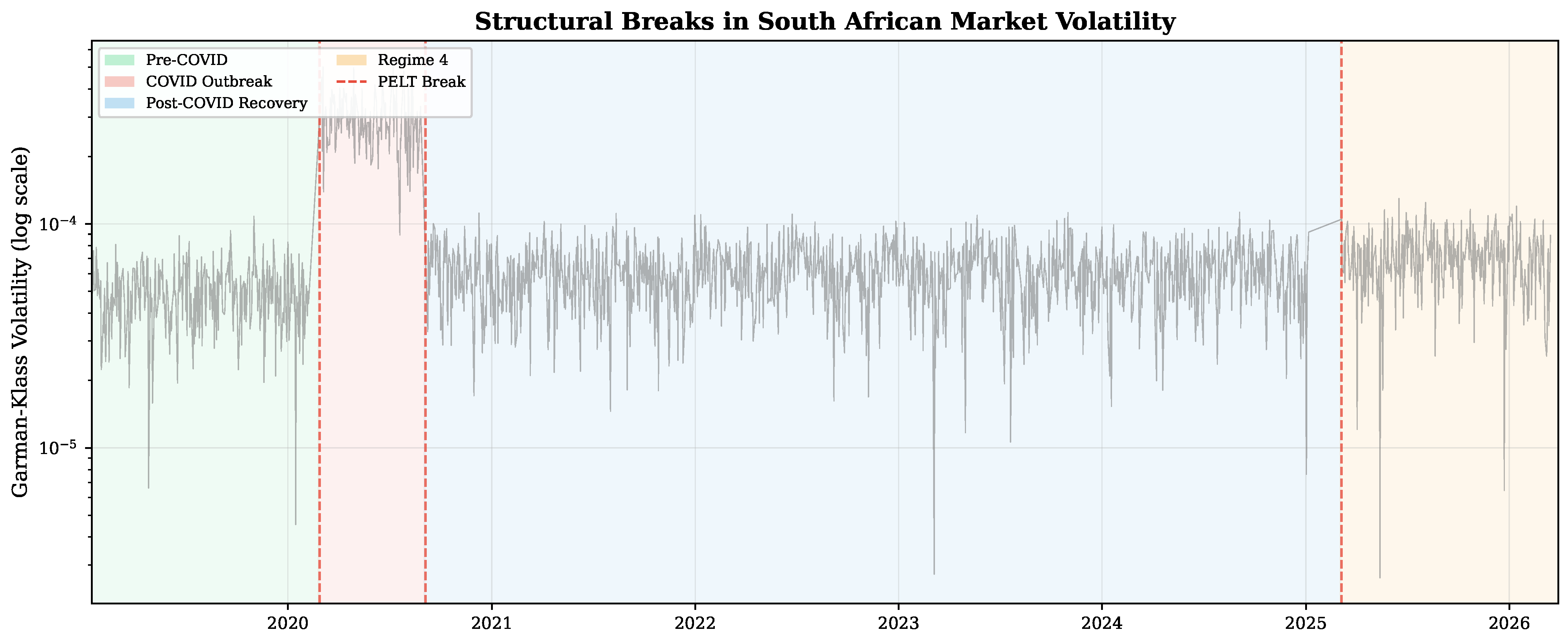
The PELT algorithm identified 15 candidate break points in the J203.JO Garman–Klass volatility series over January 2019–March 2026. We use these candidate breakpoints as local evidence of changes in log-volatility rather than as 15 separate economic regimes. The four regimes used in the EVT and forecasting analyses are therefore an interpretive aggregation of the PELT segments. The aggregation follows two rules. First, the COVID outbreak regime begins at the first PELT breakpoint associated with the sharp pandemic-era volatility increase and ends when volatility returns from the acute-crisis level. Second, adjacent post-crisis PELT segments are grouped together when they show short-lived local variation but no sustained shift in the overall volatility environment. This procedure separates local statistical breakpoints from the broader economic regimes used for interpretation. The four resulting regimes are reported in Table 2.
Table 2.
Four broad volatility regimes used in the empirical analysis. The regime boundaries are based on PELT-detected local breakpoints, with Chow tests used as complementary breakpoint checks.
Several features of the regime structure shown in Figure 2 are noteworthy. First, the onset of the COVID-19 pandemic (detected on 2020-02-27) is recovered endogenously from the volatility data alone, without reference to external epidemiological dates. The algorithm places the break twelve days before the official WHO pandemic declaration (11 March 2020), reflecting that South African markets began pricing in extreme risk slightly ahead of the formal announcement. Second, the transition out of the acute pandemic phase (2020-09-04) coincides with the relaxation of South Africa’s strictest lockdown measures and the initial economic reopening. Third, the algorithm identifies a prolonged Post-COVID Recovery regime spanning nearly five years, during which volatility remained structurally elevated relative to pre-pandemic levels but was no longer dominated by crisis-level shocks. Fourth and most critically, a fourth regime emerges in early 2025 (2025-03-06), suggesting that the South African market may have entered yet another distinct volatility environment in the most recent period.
Figure 2.
Garman–Klass volatility series with aggregated regime boundaries derived from PELT-detected local breakpoints. The dashed red lines mark the broad regime boundaries used for the EVT and forecasting analyses.
This four-regime structure represents a methodological improvement over the original study’s three qualitative periods. Whereas the original study imposed broad regime boundaries primarily through narrative interpretation, the revised approach grounds the broader interpretive regimes in PELT-detected local breakpoints, with Chow-test statistics providing complementary evidence regarding the candidate break locations (see Figure 3). The resulting regimes serve as the analytical framework for the Extreme Value Theory estimation and model evaluation that follow.
Figure 3.
Chow test F-statistics for PELT-detected candidate breakpoints in the log-transformed Garman–Klass volatility series. Green bars indicate candidate breakpoints with Chow-test statistics above the 5% critical value. The tests provide complementary evidence on local breakpoints and are not used as a separate validation of the four-regime aggregation.
5. Extreme Value Analysis of Tail Risk
5.1. POT-GPD Methodology with Inference
Standard financial risk models typically assume normally distributed returns, which systematically underestimate the frequency and magnitude of extreme market events [36]. Extreme Value Theory (EVT) addresses this limitation by focusing explicitly on the asymptotic behavior of the distribution’s tails, providing a rigorous statistical framework for quantifying tail risk without imposing parametric assumptions on the full return distribution.
We employ the Peaks-Over-Threshold (POT) method, which uses more information from extreme observations than the alternative block maxima approach. Let denote a sequence of negative daily log returns (losses). The POT method considers observations that exceed a sufficiently high threshold u. According to the Pickands–Balkema–de Haan theorem [45], as , the conditional distribution of exceedances (given ) converges to the Generalized Pareto Distribution (GPD):
where is the scale parameter governing dispersion, and is the shape parameter determining tail behavior: indicates a heavy-tailed Fréchet distribution (polynomial tail decay), corresponds to an exponential tail (Gumbel domain), and implies a bounded tail with a finite upper endpoint (Weibull domain).
We set the threshold u at the 90th percentile of negative daily returns, consistent with common practice in financial EVT applications [37]. Threshold selection in the POT framework involves balancing two competing considerations: thresholds that are too low may violate the asymptotic assumptions underlying the Generalized Pareto Distribution, whereas thresholds that are too high reduce the number of exceedances and increase estimation uncertainty. The 90th percentile provides a practical compromise between these competing objectives. It leaves enough exceedances to estimate the GPD in each regime while still focusing on the lower tail, but the shorter regimes necessarily produce imprecise tail-shape estimates. Across the four South African volatility regimes, the number of exceedances ranged from 13 to 113. To evaluate the robustness of this choice, we additionally examined alternative threshold levels and report the corresponding sensitivity analyses in Section 5.3.
Parameters are estimated via maximum likelihood. The log-likelihood function for the GPD is:
subject to and for all i. Optimization uses the Nelder-Mead algorithm with multiple random starting points to ensure convergence to the global optimum.
5.1.1. Inference on the Shape Parameter
A critical limitation of the original study was that it reported point estimates of without measures of statistical precision, leading to an unreconciled “contradiction” in which negative estimates were interpreted alongside rising VaR and ES. We address this directly by computing Hessian-based standard errors for both and , enabling formal hypothesis tests. The Hessian is evaluated numerically at the MLE, and the standard error for is . We test the null hypothesis (exponential tail) using the Wald statistic . Because several regime-specific samples contain relatively few exceedances, these Wald tests should be interpreted as approximate evidence on tail shape rather than precise tests of equality across regimes.
5.1.2. Risk Measures
For a given confidence level q (we use ), the unconditional Value-at-Risk and Expected Shortfall under the GPD are:
where n is the total number of observations and k is the number of exceedances. When , the Expected Shortfall is theoretically infinite, reflecting the absence of a finite first moment for the distribution of exceedances.
5.2. SA Tail Risk Across Regimes
Table 3 reports the GPD parameter estimates and tail risk measures for each of the four regimes identified in Section 4. The results reveal a clear and economically meaningful pattern.
Table 3.
POT-GPD estimates and tail risk measures at the 99.5% confidence level across four SA volatility regimes. Standard errors are computed from the numerical Hessian. tests .
Across the first three regimes, the estimated shape parameter is not statistically different from zero (Pre-COVID: , ; COVID: , ; Post-COVID: , ). These tests do not prove that the return tails are exactly exponential. They show that the available exceedances do not provide enough evidence to reject . The negative point estimates in the COVID and Post-COVID regimes should therefore be read as imprecise estimates rather than evidence of bounded tails.
The estimates provide no clear evidence of regime-specific changes in . By contrast, the scale parameter changes sharply across regimes. During the COVID Outbreak regime, increased from 0.0054 to 0.0351, and VaR0.995 rose from 2.91% to 9.44%. ES0.995 rose from 3.80% to 10.07%. In the Post-COVID Recovery regime, declined to 0.0068, and both VaR and ES moved back toward pre-pandemic levels. This pattern is consistent with crisis-period risk increasing mainly through the scale of extreme losses, although the regime-specific estimates are too imprecise to support a strong equality claim.
5.3. Regime 4 (2025–2026)
The fourth regime (March 2025–March 2026) gives a similar inference, but the short sample requires caution. At the 90th percentile threshold, the estimated shape parameter is (, , ), so cannot be rejected. Threshold sensitivity checks give estimates from 0.08 at the 90th percentile to 0.29 at the 95th percentile, with all p-values above 0.35. These results are compatible with an exponential tail, but they should not be read as proof of a fixed tail form.
The Regime 4 scale estimate is still informative. The scale parameter is higher than the Pre-COVID value of 0.0054, and rises to 4.65% compared with 2.91% before COVID. This increase is smaller than the COVID Outbreak spike (VaR = 9.44%), but it is consistent with Regime 4 being a distinct volatility environment. Given the limited number of exceedances, the evidence is stronger for a change in loss scale than for a change in tail shape.
5.4. Cross-Market EVT Comparison
To assess whether the South African tail-shape results are specific to one market, we replicate the POT-GPD analysis for the United States and Brazil. For each market, we estimate GPD parameters for two regimes: a Pre-COVID baseline (January 2019–February 2020) and the COVID crisis period. Table 4 reports the results.
Table 4.
Cross-market POT-GPD estimates at the 99.5% confidence level. Standard errors in parentheses. No estimate is statistically different from zero at .
The three-market EVT comparison provides two main pieces of evidence. First, the null hypothesis cannot be rejected for any of the South Africa, United States, or Brazil regime pairs reported in Table 4; all tests have and . This does not establish a common exponential tail law across markets. It indicates that, in these EVT samples, the estimated shape parameters are statistically compatible with . Even the largest point estimate, observed for the United States during COVID (), has a standard error large enough that the null is not rejected.
Second, the clearest differences across markets and regimes appear in the scale parameter , while the shape estimates are too imprecise to support strong cross-market claims about . South Africa experienced an increase in during COVID, rising from 0.0054 to 0.0338, while Brazil increased from 0.0115 to 0.0664. In contrast, the United States experienced a comparatively smaller increase from 0.0070 to 0.0129. These results suggest that commodity-exporting emerging markets experience larger increases in tail risk during global shocks than developed markets with more stable exchange rate structures.
Third, the cross-market variation in VaR and ES primarily reflects differences in volatility scale rather than differences in tail heaviness. Brazil recorded the highest COVID-period ES value at 15.33%, driven largely by its elevated estimate despite having a negative estimate. In these samples, the estimated shape parameters are statistically compatible with , while the larger crisis-period changes appear mainly in the scale parameter .
6. Cross-Market Volatility Dynamics
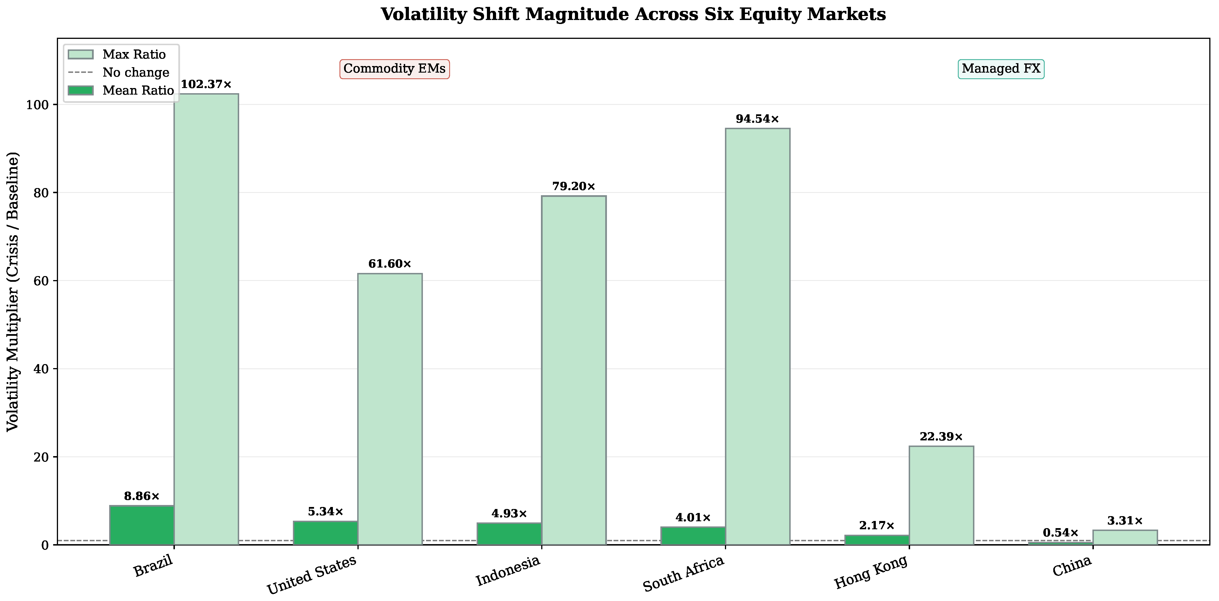
The EVT comparison in Section 5.4 was limited to South Africa, the United States, and Brazil. To broaden the cross-market evidence without extending the GPD analysis to every index, this section uses a simpler volatility-based comparison across all six markets. Specifically, we compare changes in Garman–Klass volatility between baseline and crisis periods. Table 5 reports the mean and maximum Garman–Klass volatility during the baseline and crisis periods, together with the corresponding volatility multipliers. Brazil experienced the largest mean volatility multiplier of 8.86, followed by the United States (5.34), Indonesia (4.93), South Africa (4.01), Hong Kong (2.17), and China (0.54). The largest peak volatility multipliers were observed for Brazil, South Africa, and Indonesia. China’s mean multiplier below unity indicates that average volatility during its PELT-identified crisis period was lower than during the preceding baseline, consistent with the relatively contained impact of COVID-19 on Chinese equity markets after the initial outbreak.
Table 5.
Volatility shift magnitudes across six markets. Crisis periods are market-specific and determined by PELT-detected break dates.
The cross-market comparison reveals substantial heterogeneity in volatility amplification during the COVID-19 crisis. China and Hong Kong exhibit the smallest volatility multipliers among the six markets. China’s multiplier of 0.54, the only value below unity in the sample, indicates that average GK volatility during its PELT-identified crisis period (March–October 2020) was lower than during the preceding five-year baseline. This pattern is consistent with the rapid containment of COVID-19 in China during early 2020 and the subsequent resumption of economic activity, which may have limited the duration and intensity of financial market disruption relative to other markets. Hong Kong’s multiplier of 2.17, while larger than China’s, remains below those of the commodity-exporting emerging markets and the United States. The relatively moderate volatility amplification in these two markets is consistent with the literature on managed exchange rate structures and reduced pass-through of global volatility shocks to domestic equity prices [44].
The United States recorded the second-largest mean volatility multiplier (5.34) despite having the most developed and liquid financial market in the sample. This result reflects the severity of the COVID-19 shock in the US during early 2020, when the S&P 500 experienced some of its largest daily swings on record. The US multiplier exceeds those of three commodity-exporting emerging markets (Indonesia, South Africa, and the two managed-currency economies), indicating that market development alone did not insulate against pandemic-era volatility amplification.
As shown in Figure 4, South Africa’s mean volatility multiplier of 4.01 places it in the middle of the sample, between the most affected markets (Brazil and the United States) and the least affected (Hong Kong and China). This pattern is consistent with South Africa’s dual characteristics as a commodity-exporting economy with a relatively developed financial market and floating exchange rate. The South African market absorbs global shocks through both commodity-price and capital-flow channels, though the moderate magnitude of its volatility multiplier shows that these channels did not produce amplification on the scale observed in Brazil or the United States during the COVID-19 crisis.
Figure 4.
Mean and peak Garman–Klass volatility multipliers during crisis periods relative to baseline periods across six markets.
The three-market EVT comparison and the six-market volatility-multiplier analysis lead to the same interpretation: crisis-period risk differences appear more visible on the volatility scale than in the estimated tail shape. This conclusion should be read as comparative evidence rather than as a formal equality test for GPD shape parameters across all six markets.
7. Volatility Forecasting: Model Comparison
Having established the regime structure and tail-risk characteristics of the South African market, we next evaluate the out-of-sample volatility forecasting performance of three competing models: a classical econometric GJR-GARCH model augmented with exogenous variables, a Hybrid GARCH-LSTM neural network, and an Attention-GRU baseline. The forecasting analysis serves two main purposes. First, it assesses whether deep learning models provide measurable improvements over classical econometric approaches for South African volatility forecasting. Second, it examines how forecasting difficulty varies across regimes and across markets.
7.1. Model Specifications
7.1.1. GJR-GARCH-X
The baseline model is a GJR-GARCH(1,1) specification with exogenous regressors in the variance equation (GARCH-X). Let denote the daily log return. The conditional mean and variance are:
where if and 0 otherwise.The parameter captures the leverage effect, where negative returns increase future volatility more than positive returns of equal magnitude. The exogenous variables are the daily returns on the ZAR/USD exchange rate, gold futures, and the SA repo rate. We use the Student’s t distribution for the innovations to accommodate the heavy tails documented in Section 3.3.
7.1.2. Hybrid GARCH-LSTM
The second model feeds the GJR-GARCH conditional variance estimate into a Long Short-Term Memory (LSTM) network [46]. In the first stage, a GJR-GARCH-X model is estimated on the training sample, and the fitted conditional variance is extracted. In the second stage, an LSTM network takes as input a 21-day rolling window of features: the daily log return, the three exogenous variables, and the GARCH conditional variance. The LSTM architecture consists of two layers with 64 hidden units each, dropout regularization of 0.2, and a final feedforward layer with Softplus activation to ensure positive variance predictions. The model is trained to minimize the QLIKE loss function directly, aligning the training objective with the forecast evaluation metric.
The hybrid design combines the strengths of the two approaches. GARCH captures volatility clustering and leverage effects in a parsimonious parametric framework, while the LSTM can learn nonlinear interactions and regime-dependent dynamics that may not be captured by the linear GARCH-X specification. By providing the GARCH variance as an input feature, we give the LSTM a strong prior on the conditional variance structure, reducing the data requirements relative to a purely data-driven deep learning approach.
7.1.3. Attention-GRU
As a second deep learning baseline, we implement a Gated Recurrent Unit (GRU) network with an attention mechanism over the temporal dimension [47]. The architecture mirrors the LSTM: two GRU layers with 64 hidden units, attention-pooling of the hidden states, and a Softplus output layer. The GRU is trained on the same 21-day rolling windows and the same feature set as the LSTM. As reported in Section 7.4, the Attention-GRU records the lowest QLIKE in both Test A and Test B on the aligned evaluation samples. Its improvement over GJR-GARCH-X is marginally significant in Test A (, ) and in Test B (, ), but neither comparison reaches the 5% level.
The deep learning architectures were implemented using a common set of hyperparameters selected from values widely adopted in the financial time-series literature. Because the primary objective of this study is comparative evaluation rather than architecture optimization, extensive hyperparameter tuning was not performed. The same network configuration was maintained across all experiments to ensure consistency and facilitate direct comparison with the econometric benchmark.
All preprocessing and model-selection choices were made within the training design for each experiment. Feature scaling, rolling-window construction, early stopping, and neural-network training used only the training sample and, where applicable, an internal validation split from that training sample. The test periods were not used to tune hyperparameters, choose stopping points, rescale features, or modify model specifications.
7.2. Forecasting Design
We evaluate model performance under two out-of-sample scenarios, mirroring the practical forecasting problem faced by risk managers:
- Test A (Crisis Generalization): Train on Pre-COVID regime (280 days, January 2019–February 2020), test on COVID Outbreak regime (130 days, February–September 2020). This tests whether models trained on calm-market data can generalize to crisis conditions, which is the scenario most relevant for risk management.
- Test B (New Normal Generalization): Train on Pre-COVID + COVID Outbreak (410 days combined, January 2019–September 2020), test on the usable Post-COVID Recovery forecasting sample (1124 observations before the 21-day neural-network alignment window, September 2020–March 2025). This tests whether models trained on pre-2020 data can forecast volatility in the post-pandemic new normal.
All forecasting models use the same training and testing periods, forecast horizon, and input variables. The GJR-GARCH-X, Hybrid GARCH-LSTM, and Attention-GRU models are estimated within the relevant training window and then evaluated on held-out observations. No model is re-estimated or tuned using test-period outcomes. The deep learning architectures employed the same input features, rolling window length (21 trading days), optimization procedure, and early stopping criterion across all experiments. Consequently, differences in forecasting performance reflect differences in model structure rather than differences in the evaluation protocol. All models are evaluated against the Garman–Klass volatility proxy using two complementary loss functions: Mean Squared Error (MSE) and Quasi-Likelihood (QLIKE) loss [26]. QLIKE is the preferred metric in the volatility forecasting literature because it is robust to noise in the volatility proxy and asymmetrically penalizes under-prediction, which is the more costly error for risk management applications.
7.3. Diebold–Mariano Test
To determine whether observed differences in forecast accuracy are statistically significant, we employ the Diebold-Mariano (DM) test of equal predictive accuracy [43]. For two competing forecasts producing loss differentials , the DM statistic tests . We use the QLIKE loss function, a heteroskedasticity-and-autocorrelation-consistent (HAC) estimator of the variance with lags, and a two-sided alternative. In Table 6, the GJR-GARCH-X model is the reference model for the reported DM statistics. A positive DM statistic means that the GARCH baseline has a larger QLIKE loss than the competing model.
Table 6.
Out-of-sample volatility forecasting performance on cleaned data. DM statistics compare each competing model against GJR-GARCH-X using QLIKE loss. A positive DM statistic indicates that GJR-GARCH-X has the larger loss.
Although the Diebold–Mariano test is widely used for comparing forecast accuracy, its asymptotic validity assumes that the loss differential series is covariance stationary with weak temporal dependence. These assumptions may be affected by structural breaks and periods of heightened volatility. To mitigate this concern, the DM tests are performed separately within the predefined out-of-sample evaluation periods rather than across the full sample, thereby reducing the influence of regime changes on the loss differential. Consequently, the reported p-values should be interpreted as evidence of relative predictive performance within each evaluation period rather than as universally applicable across all market conditions.
7.4. Forecasting Results
Table 6 reports the out-of-sample MSE and QLIKE for all three models across both test scenarios.
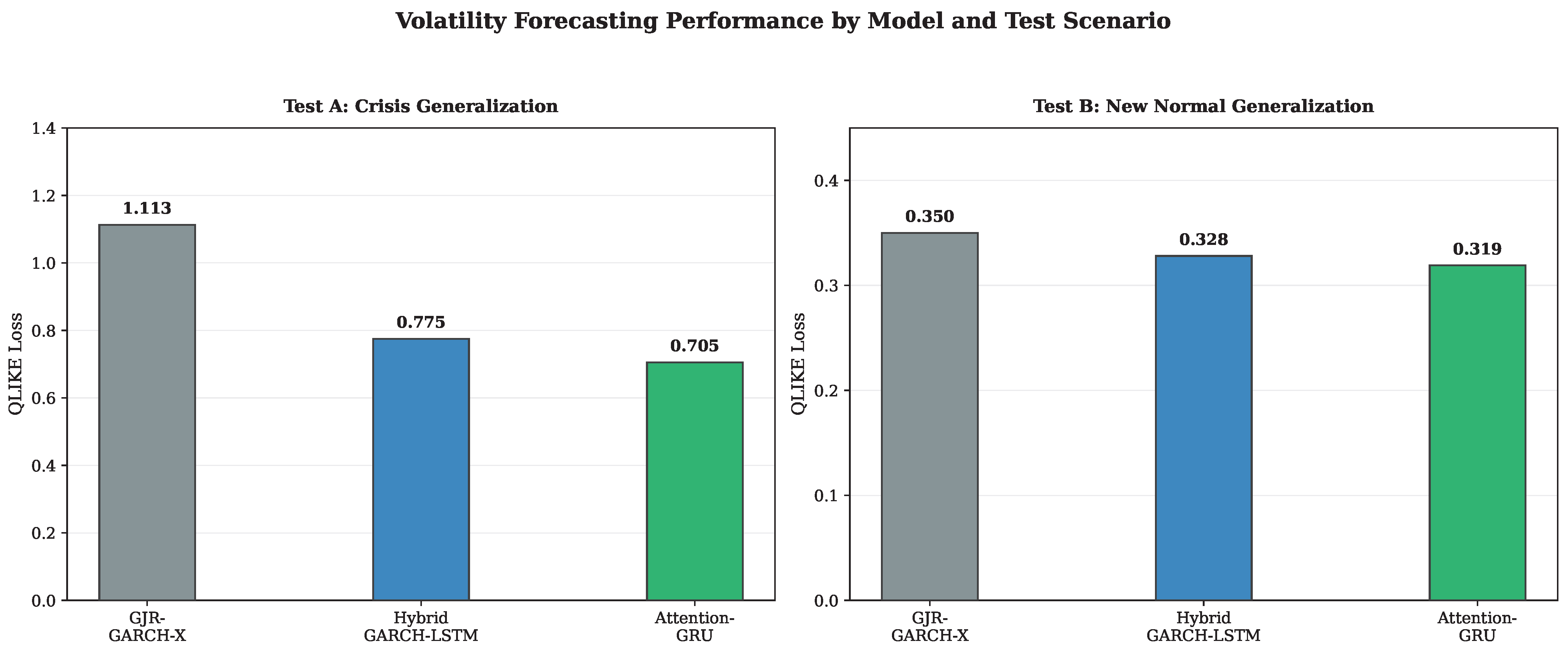
Figure 5 shows the QLIKE loss results. In Test A, both neural-network models reduce QLIKE relative to GJR-GARCH-X on the aligned evaluation sample. GJR-GARCH-X records QLIKE of 1.113, compared with 0.775 for the Hybrid GARCH-LSTM and 0.705 for the Attention-GRU. The LSTM improvement is not statistically significant (, ). The GRU improvement is marginal at the 10% level (, ).
Figure 5.
QLIKE loss by model and test scenario on the cleaned dataset. Lower values indicate better forecast accuracy. On the aligned evaluation samples, the Attention-GRU records the lowest QLIKE in both Test A (0.705) and Test B (0.319). The Hybrid GARCH-LSTM significantly improves on GJR-GARCH-X in Test B (, ), while the GRU improvements are marginal at the 10% level in both tests.
In Test B, all models have lower QLIKE values than in Test A. The Attention-GRU again records the lowest QLIKE (0.319), followed by the Hybrid GARCH-LSTM (0.328) and GJR-GARCH-X (0.350). The LSTM improvement over GJR-GARCH-X is statistically significant at the 5% level (, ). The GRU improvement is marginal at the 10% level (, ).
The aligned-sample results qualify the model comparison. Both neural-network models reduce QLIKE in both test windows, but the statistical evidence is uneven. The LSTM improvement is significant at the 5% level only in Test B, while the GRU has the lowest QLIKE values but only marginal DM evidence against the GARCH baseline.
7.5. Expanding-Window Cross-Validation
To assess the stability of the GJR-GARCH-X model across the post-COVID period, we conduct an expanding-window cross-validation exercise. Starting from an initial training window of 504 days (approximately two years), we expand the training set by 126 days (six months) at each step and forecast the subsequent 126-day test window. Windows where the QLIKE exceeds 10 are flagged as diverged and excluded.
Table 7 reports the results of the analysis. All seven expanding-window evaluations produce stable forecasts, with QLIKE values ranging from 0.30 to 0.56 (mean , ). No window exceeds the divergence threshold of . Window 6 (March–September 2025) yields a QLIKE of 0.56, modestly above the cross-window mean but within the range of normal forecast variation.
Table 7.
Expanding-window cross-validation: GJR-GARCH-X on Post-COVID SA data. All seven windows produce stable forecasts.
The stability of GJR-GARCH-X across all seven windows indicates that the post-COVID volatility environment does not contain a period of catastrophic forecast failure under this evaluation design. This finding is consistent with the broader evidence that post-COVID risk changes are more visible in the volatility scale than in statistically clear shifts in the estimated GPD shape parameter.
7.6. Cross-Market Benchmark: SA vs. US
A natural question is whether the forecasting difficulty we observe for South Africa is specific to this market or reflects a general challenge in volatility forecasting. To answer this, we estimate the identical GJR-GARCH-X specification on S&P 500 data, using US-specific exogenous variables (USD Index returns, gold returns, and the Federal Funds rate).
On S&P 500 data, the GJR-GARCH-X model achieves in Test A (crisis generalization) and in Test B (new normal). The corresponding SA values are 1.019 and 0.350. The pattern differs between the two tests. During the crisis period, SA QLIKE exceeds the US value by a factor of approximately 1.9, consistent with the greater volatility amplification observed in emerging markets during global shocks. In the post-crisis period, SA QLIKE of 0.350 is lower than the US value of 0.491.
During the COVID-19 crisis, the SA GJR-GARCH-X QLIKE was about 1.9 times the corresponding US value under the same model specification and loss function. In the post-crisis period, the SA QLIKE was lower than the US value. This pattern shows that the SA–US forecasting gap is concentrated in the crisis evaluation window rather than persisting across both test periods.
8. Discussion
This study investigated whether the COVID-19 pandemic produced only a temporary disruption in the South African stock market or whether it induced more persistent structural changes in market risk dynamics. The findings provide evidence that volatility behavior in the South African market changed during and after the pandemic period, with important implications for tail-risk estimation and volatility forecasting in emerging markets. The results are broadly consistent with prior studies documenting heightened volatility and instability during the COVID-19 period in African and emerging financial markets [15,16,24]. However, whereas much of the existing literature focuses primarily on the immediate pandemic shock, the present study extends the analysis into the post-pandemic period and provides evidence that volatility dynamics in the South African market did not fully revert to their pre-pandemic behavior after 2022.
In the South African regime analysis and the three-market EVT comparison, the estimated GPD shape parameters are not statistically different from zero. This means that the EVT samples considered here do not provide clear evidence of a shift away from . The larger changes appear in the scale parameter , especially during the COVID-19 period. This pattern is clearest for South Africa and Brazil, where the estimated scale of extreme losses increased more sharply than in the United States.
The regime-specific estimates are compatible with an exponential tail specification, including in the most recent 2025–2026 regime. Given the small number of exceedances in some regimes, this result should be interpreted cautiously. The evidence is stronger for changes in the scale of extreme losses than for changes in the tail index.
The forecasting analysis further indicates that the relative difficulty of forecasting South African market volatility depends on the prevailing market regime. During the COVID-19 crisis, SA volatility was approximately 1.9 times harder to forecast than US volatility under identical model specifications, consistent with the greater volatility amplification observed in commodity-exporting emerging markets during global shocks. In the post-crisis period, however, GJR-GARCH-X performed comparably across the two markets, with SA Test B QLIKE of 0.350 slightly below the corresponding US value of 0.491. This shows that the forecasting gap between emerging and developed markets is concentrated in crisis episodes rather than persisting uniformly across all market conditions.
The forecasting results are mixed. Both neural-network specifications reduce QLIKE relative to GJR-GARCH-X on the aligned samples. The Hybrid GARCH-LSTM improvement is significant at the 5% level in Test B (). The Attention-GRU has the lowest QLIKE in both tests, but its improvements over GJR-GARCH-X are marginal at the 10% level. Given the simpler GJR-GARCH-X benchmark, the evidence supports a limited conclusion: neural networks improve forecast loss in some settings, but the gains are not equally strong across models and test periods.
Limitations
Several limitations should be considered when interpreting the findings of this study. First, although the PELT algorithm and Chow-test validation provide a statistically supported framework for identifying structural breaks, alternative breakpoint detection methods or penalty choices may produce different regime boundaries. Sensitivity analyses indicated that the principal volatility regimes remained broadly consistent across reasonable parameter choices, although minor breakpoint locations varied. Second, the EVT analysis depends on the selection of the threshold in the Peaks-over-Threshold framework. Although sensitivity analyses using alternative threshold levels produced qualitatively similar conclusions, formal threshold diagnostic tools, such as mean residual life and parameter stability plots, were not included. Future work could incorporate these diagnostics to further strengthen threshold selection.
Third, the interpretation of the 2025–2026 regime should be regarded as preliminary. This regime spans approximately 13 months and contains 27 exceedances at the 90th percentile threshold, comparable to the Pre-COVID and COVID regimes but with wider confidence intervals for the estimated tail parameters. While the PELT algorithm identifies this as a distinct volatility environment, the EVT analysis indicates that tail behavior remains consistent with the exponential pattern observed across all other regimes. Additional observations are required to determine whether this regime represents a persistent structural change or a temporary episode. Fourth, the cross-market comparison involves differences in sample size and market history. In particular, the South African dataset contains fewer observations than several of the developed markets, which may influence breakpoint detection, EVT parameter estimation, and forecast evaluation. Consequently, the cross-market results should be interpreted primarily as comparative evidence rather than precise quantitative rankings.
Finally, the forecasting analysis considers a set of econometric and deep learning models using a common set of exogenous variables. Other model architectures, additional macroeconomic or country-specific risk factors, and alternative training strategies may yield different forecasting performance. The objective of this study is therefore not to identify a universally optimal forecasting model, but rather to evaluate representative modeling approaches under a consistent experimental framework.
9. Conclusions
This study investigated volatility regime shifts and tail-risk dynamics in the South African stock market using structural break detection, Extreme Value Theory, and volatility forecasting models across six equity markets. Three findings emerge from the analysis.
First, the EVT estimates are statistically compatible with across the South African regimes and in the three-market comparison with the United States and Brazil. The analysis does not prove that tail behavior is identical across regimes or markets. It does show that the main changes in VaR and Expected Shortfall are more closely associated with changes in the scale parameter than with statistically clear shifts in tail shape. Second, the magnitude of volatility amplification during the COVID-19 crisis varied substantially across markets. Brazil recorded the largest mean volatility multiplier of 8.86, followed by the United States (5.34), Indonesia (4.93), and South Africa (4.01). Hong Kong (2.17) and China (0.54) exhibited the smallest multipliers, with China’s value below unity indicating that average volatility during its crisis period was lower than during the preceding baseline. The ranking does not follow a simple developed-versus-emerging market division, suggesting that country-specific factors, including economic structure, pandemic containment measures, and exchange rate arrangements, shaped the intensity of financial market disruption.
Third, the relative difficulty of forecasting South African market volatility depends on the prevailing market regime. During the COVID-19 crisis, South Africa produced a substantially larger forecasting loss than the United States under the selected QLIKE metric and otherwise identical model specifications. In the post-crisis period, the GJR-GARCH-X model performed comparably across the two markets, with SA Test B QLIKE of 0.350 below the US value of 0.491. The Hybrid GARCH-LSTM and Attention-GRU both reduce QLIKE relative to GJR-GARCH-X on aligned samples. The LSTM improvement is statistically significant in the post-crisis Test B window, while the GRU records the lowest QLIKE values but only marginal DM evidence against the GARCH baseline. Overall, crisis-period risk changes in this sample are more visible in volatility scale than in statistically clear shifts in tail shape. They also show that PELT-based local breakpoint detection, combined with transparent regime aggregation, can provide a useful framework for studying emerging-market volatility, and that the SA–US forecasting gap depends on the evaluation period rather than appearing uniformly across regimes.
Author Contributions
Conceptualization, C.H. and G.O.; methodology, C.H. and G.O.; investigation, G.O., E.E., C.H. and C.M.; resources, G.O.; writing—original draft preparation, C.H. and G.O.; writing—review and editing, G.O., E.E., C.H. and C.M.; visualization, G.O., E.E., C.H. and C.M.; supervision, C.H. and G.O. All authors have read and agreed to the published version of the manuscript.
Funding
This research received no external funding.
Data Availability Statement
The data presented in this study are publicly available from Yahoo Finance (https://finance.yahoo.com/) and were accessed using the Python 1.5.1 yfinance library (version 1.5.1). The processed datasets and code used for the analysis are available from the corresponding author upon reasonable request.
Conflicts of Interest
The authors declare no conflicts of interest.
Abbreviations
The following abbreviations are used in this manuscript:
| AI | Artificial Intelligence |
| ARCH-LM | Autoregressive Conditional Heteroskedasticity Lagrange Multiplier |
| COVID-19 | Coronavirus Disease 2019 |
| DM | Diebold–Mariano |
| EM | Emerging Market |
| ES | Expected Shortfall |
| EVT | Extreme Value Theory |
| FRED | Federal Reserve Economic Data |
| GARCH | Generalized Autoregressive Conditional Heteroskedasticity |
| GK | Garman–Klass |
| GPD | Generalized Pareto Distribution |
| GRU | Gated Recurrent Unit |
| GJR-GARCH | Glosten–Jagannathan–Runkle GARCH |
| HAC | Heteroskedasticity and Autocorrelation Consistent |
| HK | Hong Kong |
| JSE | Johannesburg Stock Exchange |
| LSTM | Long Short-Term Memory |
| MLE | Maximum Likelihood Estimation |
| MSE | Mean Squared Error |
| OHLC | Open, High, Low, Close |
| PELT | Pruned Exact Linear Time |
| POT | Peaks Over Threshold |
| QLIKE | Quasi-Likelihood |
| RSS | Residual Sum of Squares |
| SA | South Africa |
| SE | Standard Error |
| VaR | Value-at-Risk |
| WHO | World Health Organization |
References
- Tabash, M.I.; Chalissery, N.; Nishad, T.M.; Al-Absy, M.S.M. Market shocks and stock volatility: Evidence from emerging and developed markets. Int. J. Financ. Stud. 2024, 12, 2. [Google Scholar] [CrossRef] [Scilit]
- Molina-Muñoz, J.E.; Soriano-Felipe, P. Dynamic spillovers among policy uncertainty, financial markets and energy markets in developed and emerging economies. Econ. Change Restruct. 2026, 59, 7. [Google Scholar]
- Negi, P.; Jaiswal, A. Impact of ROBO Global Robotics and Automation Index ETF on stock market dynamics in emerging economies. Bottom Line 2026. Epub ahead of printing. [Google Scholar] [CrossRef] [Scilit]
- Pessoa, G.H.R.; Rochman, R.R. Macro-Financial Blind Spots in Emerging Markets: Non-Bank Intermediation, Funding Liquidity, and the Persistence of Global Shock Transmission. Int. J. Financ. Stud. 2026, 14, 40. [Google Scholar] [CrossRef] [Scilit]
- Yousfani, K.; Iftikhar, H.; Rodrigues, P.C.; Armas, E.A.T.; López-Gonzales, J.L. Global shocks and local fragilities: A financial stress index approach to pakistan’s monetary and asset market dynamics. Economies 2025, 13, 243. [Google Scholar] [CrossRef] [Scilit]
- Aljughaiman, A.A.; Tabash, M.I.; Issa, S.S.; Almulhim, A.A. Shock transmission from global financial stress, bitcoin sentiment indices, US and euro financial market uncertainty toward the GCC stock volatility. Cogent Bus. Manag. 2025, 12, 2514811. [Google Scholar] [CrossRef] [Scilit]
- Wątorek, M.; Kwapień, J.; Drożdż, S. Financial Return Distributions: Past, Present, and COVID-19. Entropy 2021, 23, 884. [Google Scholar] [CrossRef] [Scilit] [PubMed]
- Gherghina, S.C.; Constantinescu, C.A. Towards examining the volatility of top market-cap cryptocurrencies throughout the COVID-19 outbreak and the Russia–Ukraine war: Empirical evidence from GARCH-type models. Risks 2025, 13, 57. [Google Scholar] [CrossRef] [Scilit]
- Emam, H.A. Examining monetary policy cyclicality in Egypt during crisis time: Global financial crisis versus COVID-19 pandemic. Int. J. Econ. Financ. Issues 2024, 14, 107. [Google Scholar] [CrossRef] [Scilit]
- Iyke, B.N.; Ho, S.Y. Exchange rate exposure in the South African stock market before and during the COVID-19 pandemic. Financ. Res. Lett. 2021, 43, 102000. [Google Scholar] [CrossRef] [Scilit] [PubMed]
- Kita, S.M.; Sparkes, E.; Cotti, D.; Hagenlocher, M. A Nation of Disasters: Lessons on Systemic Risks and Cascading Impacts from Malawi’s COVID-19 Experience. Risk Anal. 2026, 46, e70229. [Google Scholar] [CrossRef] [Scilit] [PubMed]
- Ndlovu, N. The Impact of Macroeconomic Variables on the Johannesburg Stock Exchange (JSE) Indices. Master’s Thesis, University of Cape Town, Cape Town, South Africa, 2023. [Google Scholar]
- Ayadi, O.F.; Williams, J. Stock market development and capital formation in selected African economies. J. Money Bus. 2023, 3, 125–136. [Google Scholar] [CrossRef] [Scilit]
- Zondi, M.; Phesa, M.; Nutassey, V.A. Impact of economic shocks in the Johannesburg Stock Exchange 15 index prices. Int. J. Res. Bus. Soc. Sci. 2025, 14, 225. [Google Scholar]
- Ramakau, T.; Mokatsanyane, D.; Matlhaku, K.; Ferreira-Schenk, S. Analyzing the South African Equity Market Volatility and Economic Policy Uncertainty During COVID-19. Economies 2025, 13, 276. [Google Scholar] [CrossRef] [Scilit]
- Vengesai, E. COVID-19 and stock market volatility in South Africa: A cross-sector analysis. Asian Econ. Financ. Rev. 2022, 12, 473–493. [Google Scholar] [CrossRef] [Scilit]
- Baek, S.W.; Mohanty, S.K.; Glambosky, M. COVID-19 and stock market volatility: An industry-level analysis. Financ. Res. Lett. 2020, 37, 101748. [Google Scholar] [CrossRef] [Scilit] [PubMed]
- Engle, R.F.; Giglio, S.; Kelly, B.; Lee, H.; Stroebel, J. Hedging climate change news. Rev. Financ. Stud. 2020, 33, 1184–1216. [Google Scholar] [CrossRef] [Scilit]
- Fischer, T.; Krauss, C. Deep learning with long short-term memory networks for financial market predictions. Eur. J. Oper. Res. 2018, 270, 654–669. [Google Scholar] [CrossRef] [Scilit]
- Oktaviana, P.P.; Syafei, A.D.; Kuswanto, H.; Hermana, J. Extreme Value Theory for Climate-Related Environmental Disaster Risk Analysis: A Review of Urban Impacts and Vulnerabilities. Future Cities Environ. 2026, 12, 19. [Google Scholar] [CrossRef] [Scilit]
- Shah, S.A.; Raza, H.; Mustafa Hashmi, A. Downside risk-return volatilities during COVID-19 outbreak: A comparison across developed and emerging markets. Environ. Sci. Pollut. Res. 2022, 29, 70179–70191. [Google Scholar] [CrossRef] [Scilit]
- Gunay, S.; Can, G. The source of financial contagion and spillovers: An evaluation of the COVID-19 pandemic and the global financial crisis. PLoS ONE 2022, 17, e0261835. [Google Scholar] [CrossRef] [Scilit] [PubMed]
- Jing, W.L.; Rashid, S.B.A.; Islam, M.U. The impact of COVID-19 on financial markets & institutions: A literature review. Int. J. Early Child. Spec. Educ. 2022, 14, 6488–6502. [Google Scholar]
- Del Lo, G.; Basséne, T.; Séne, B. COVID-19 and the African Financial Markets: Less Infection, Less Economic Impact? Financ. Res. Lett. 2022, 45, 102148. [Google Scholar] [CrossRef] [Scilit] [PubMed]
- Ncube, M.; Sibanda, M.; Matenda, F.R. Investigating the effects of the COVID-19 pandemic on stock volatility in Sub-Saharan Africa: Analysis using Explainable Artificial intelligence. Economies 2024, 12, 112. [Google Scholar] [CrossRef] [Scilit]
- Patton, A.J. Volatility forecast comparison using imperfect volatility proxies. J. Econom. 2011, 160, 246–256. [Google Scholar] [CrossRef] [Scilit]
- Garman, M.B.; Klass, M.J. On the Estimation of Security Price Volatilities from Historical Data. J. Bus. 1980, 53, 67–78. [Google Scholar] [CrossRef] [Scilit]
- Andreou, E.; Ghysels, E. Structural breaks in financial time series. In Handbook of Financial Time Series; Springer: Berlin/Heidelberg, Germany, 2009; pp. 839–870. [Google Scholar]
- Muthuramu, P.; Maheswari, T.U. Tests for structural breaks in time series analysis: A review of recent development. Shanlax Int. J. Econ. 2019, 7, 66–79. [Google Scholar] [CrossRef] [Scilit]
- Aue, A.; Horváth, L. Structural breaks in time series. J. Time Ser. Anal. 2013, 34, 1–16. [Google Scholar]
- Babikir, A.; Gupta, R.; Mwabutwa, C. Structural breaks and GARCH models of stock return volatility: The case of South Africa. Econ. Model. 2012, 29, 2435–2443. [Google Scholar] [CrossRef] [Scilit]
- Bai, J.; Perron, P. Estimating and Testing Linear Models with Multiple Structural Changes. Econometrica 1998, 66, 47–78. [Google Scholar] [CrossRef] [Scilit]
- Bai, J.; Perron, P. Computation and Analysis of Multiple Structural Change Models. J. Appl. Econom. 2003, 18, 1–22. [Google Scholar]
- Killick, R.; Fearnhead, P.; Eckley, I.A. Optimal Detection of Changepoints with a Linear Computational Cost. J. Am. Stat. Assoc. 2012, 107, 1590–1598. [Google Scholar] [CrossRef] [Scilit]
- Chow, G.C. Tests of Equality Between Sets of Coefficients in Two Linear Regressions. Econometrica 1960, 28, 591–605. [Google Scholar] [CrossRef] [Scilit]
- Embrechts, P.; Klüppelberg, C.; Mikosch, T. Modelling Extremal Events: For Insurance and Finance; Springer Science & Business Media: Berlin/Heidelberg, Germany, 1997. [Google Scholar] [CrossRef] [Scilit]
- McNeil, A.J.; Frey, T. Estimation of Tail-Related Risk Measures for Heteroscedastic Financial Time Series: An Extreme Value Approach. J. Empir. Financ. 2000, 7, 271–300. [Google Scholar] [CrossRef] [Scilit]
- Gençay, R.; Selçuk, F. Extreme value theory and value-at-risk: Relative performance in emerging markets. Int. J. Forecast. 2004, 20, 287–303. [Google Scholar] [CrossRef] [Scilit]
- Kakade, K.; Jain, I.; Mishra, A.K. Value-at-Risk forecasting: A hybrid ensemble learning GARCH-LSTM based approach. Resour. Policy 2022, 78, 102903. [Google Scholar] [CrossRef] [Scilit]
- Maingo, I.; Ravele, T.; Sigauke, C. Volatility Modelling of the JSE Top40 Index: Assessing the GAS Framework Against GARCH and Hybrid GARCH–XGBoost. J. Risk Financ. Manag. 2025, 18, 679. [Google Scholar] [CrossRef] [Scilit]
- Dixon, M.F.; Halperin, I.; Bilokon, P. Machine Learning in Finance: From Theory to Practice; Springer: Cham, Switzerland, 2020. [Google Scholar] [CrossRef] [Scilit]
- López de Prado, M. Advances in Financial Machine Learning; John Wiley & Sons: New York, NY, USA, 2018. [Google Scholar]
- Diebold, F.X.; Mariano, R.S. Comparing Predictive Accuracy. J. Bus. Econ. Stat. 1995, 13, 253–263. [Google Scholar] [CrossRef] [Scilit]
- Calvo, G.A.; Reinhart, C.M. Fear of Floating. Q. J. Econ. 2002, 117, 379–408. [Google Scholar] [CrossRef] [Scilit]
- Balkema, A.A.; de Haan, L. Residual Life Time at Great Age. Ann. Probab. 1974, 2, 792–804. [Google Scholar] [CrossRef] [Scilit]
- Hochreiter, S.; Schmidhuber, J. Long Short-Term Memory. Neural Comput. 1997, 9, 1735–1780. [Google Scholar] [CrossRef] [Scilit] [PubMed]
- Cho, K.; van Merriënboer, B.; Gulcehre, C.; Bahdanau, D.; Bougares, F.; Schwenk, H.; Bengio, Y. Learning Phrase Representations Using RNN Encoder-Decoder for Statistical Machine Translation. In Proceedings of the 2014 Conference on Empirical Methods in Natural Language Processing (EMNLP), Doha, Qatar, 25–29 October 2014; pp. 1724–1734. [Google Scholar]

Disclaimer/Publisher’s Note: The statements, opinions and data contained in all publications are solely those of the individual author(s) and contributor(s) and not of MDPI and/or the editor(s). MDPI and/or the editor(s) disclaim responsibility for any injury to people or property resulting from any ideas, methods, instructions or products referred to in the content. |
© 2026 by the authors. Licensee MDPI, Basel, Switzerland. This article is an open access article distributed under the terms and conditions of the Creative Commons Attribution (CC BY) license.