


Abstract
Shipwreck segmentation in side-scan sonar imagery remains challenging. This study investigates whether repeating a frozen encoder block can improve the Segment Anything Model (SAM) for this task and how to select the block without labelled validation masks. The proposed Repeated-Block Segment Anything Model (RB-SAM) executes one encoder block once more while retaining all pretrained weights. The Graph Transport-to-Expansion Efficiency (GTEE) score selects the repeat location from unlabelled reference images. It uses graph energy to quantify spatial variation in features and evaluates the energy reduction at the encoder output relative to the local expansion introduced by repetition. Under stated assumptions on feature preservation, perturbation contraction and decoder margins, the theoretical analysis connects energy reduction to pixel-error correction and improved mask overlap. In the main AI4Shipwrecks experiment, GTEE selected the best-performing configuration among the 12 candidates. With identical ground-truth bounding-box prompts, the selected RB-SAM variant achieved a five-fold mean best-score intersection over union (IoU) of 31.85%, compared with 26.60% for SAM. Ablation experiments showed that local-expansion normalisation was essential to this selection. These findings support encoder block repetition with label-free configuration selection as an approach to improving frozen SAM for shipwreck segmentation without additional training.
Keywords:
side-scan sonar; imagery; marine archaeology; Segment Anything Model; graph Dirichlet energy; repeated computation; image segmentation MSC:
68T45; 68T07; 05C50; 62G35
1. Introduction
As an underwater detection sensor, side-scan sonar (SSS) is widely used to locate and document shipwrecks, supporting the study of underwater cultural heritage [1,2,3]. Shipwreck segmentation identifies the image regions occupied by a wreck and provides a pixel-wise description of its extent. However, accurate shipwreck segmentation in SSS imagery remains challenging because of speckle noise, acoustic shadows, seabed clutter, and range-dependent variations in spatial resolution [4,5,6]. Recognising wrecks partly buried by sand or sediment, fragmented remains, and fractured hulls calls for high-level semantic understanding of wreck structure and its spatial context [2]. In addition, developing supervised segmentation models requires reference masks that distinguish shipwreck pixels from the surrounding seabed. Producing these pixel-wise annotations requires substantial manual effort and specialist expertise, limiting the availability of labelled data for model development and evaluation [7]. There is therefore a need for methods that improve shipwreck segmentation while reducing dependence on task-specific manual annotations.
The need to recognise partly buried wrecks, fragmented remains, and fractured hulls by interpreting incomplete structures and their spatial context motivates this study to adapt a large pretrained foundation model and use its broad visual representations rather than develop a smaller task-specific segmentation network. For instance, the Segment Anything Model (SAM) is a promptable segmentation model that generates object masks from spatial cues, such as points or bounding boxes [8]. Its image encoder extracts visual features, its prompt encoder represents the supplied cues, and its mask decoder combines this information to predict segmentation masks. It has also demonstrated zero-shot transfer to new images and tasks without additional task-specific training. Nevertheless, SSS imagery represents acoustic returns rather than optical appearance, and its imaging geometry and shadow formation differ from those of conventional photographs [9]. This motivates investigating how SAM’s pretrained representations can be used more effectively for shipwreck segmentation while retaining its existing weights.
Optical images record reflected light, whereas SSS images record acoustic backscatter as a function of travel time and survey position. For a pulse-duration-limited SSS system, the ground-range resolution can be expressed as Ry = c tp/(2 cos β), and the along-track resolution as Rx = D sin θh, where c is sound speed, tp is pulse duration, β is the grazing angle, D is the target range, and θₕ is the horizontal beamwidth [3]. At a fixed beamwidth, doubling the range doubles the along-track resolution distance and reduces the separability of nearby structures. Acoustic shadows arise where an object blocks insonification, so their extent depends on object relief and viewing geometry [3,9]. These effects, together with speckle and the absence of independent colour channels, contribute to the general shift from optical to sonar imagery.
Shipwreck segmentation adds a semantic difficulty to this imaging shift. The foreground may consist of disconnected hull fragments or partly buried structures whose membership in the same wreck must be inferred from shape and spatial context [2]. A strong acoustic boundary may separate a highlight from its shadow or a wreck from seabed clutter, but it does not by itself identify the annotated wreck extent. The task therefore requires both accommodation of sonar image formation and recognition of incomplete wreck structure.
One possible approach is to modify the computation performed during inference rather than update the pretrained parameters. Exploratory work on repeated computation has reported that traversing selected Transformer layers more than once can improve performance in particular settings without modifying their weights. The RYS report investigates this approach in language models [10], while a recent study applies circuit duplication to a frozen visual Transformer for marine species classification [11]. Building on these findings, this study investigates whether repeated execution within SAM’s image encoder can also improve shipwreck segmentation without task-specific retraining, and block repetition is chosen here to study adaptation with a fixed checkpoint and no parameter optimisation.
Testing this possibility requires specifying which part of the encoder is repeated. Repeating sequences of encoder blocks (EBs) of different lengths would vary several aspects of the computation simultaneously [12]. To examine the effect of repeat location under a fixed repetition rule, this study restricts each candidate configuration to a single additional execution of one EB. Specifically, the selected block is reapplied to its own output before processing continues through any remaining EBs, with all pretrained weights kept frozen. This design introduces no new trainable parameters and requires no additional training. In SAM’s Vision Transformer-Base (ViT-B) image encoder, the input representation passes through 12 successive EBs, each of which transforms the intermediate image features [8]. Repeating different blocks changes the representation at different stages of the encoder [13]. The resulting representation then passes through any remaining EBs, whose number and identity depend on the repeat location. The 12 possible repeat locations therefore define 12 candidate model configurations that differ only in the location of the additional block execution. Within this set of 12 candidates, the next question is how to identify a useful repeat location.
A direct way to choose among the 12 candidate configurations is to compare their predicted masks with expert-annotated reference masks and select the configuration with the highest segmentation accuracy. Although all model weights remain frozen, this approach still relies on labelled masks to determine which EB to repeat. To remove this dependence at the block-selection stage, this study introduces a method for selecting a useful repeated block (RB) from a small, fixed set of unlabelled reference images by assessing changes in encoder features on a graph constructed from each input image.
To be more specific, without reference masks, one possible basis for comparison is the change that each RB produces in the encoder’s feature representations. Graph signal processing provides a way to describe spatial variation by treating feature locations as graph vertices and their relationships as weighted edges [14]. The associated graph Dirichlet energy [15] measures weighted differences between features at connected locations, which means that when the graph is constructed from the input image, this energy can be computed from the encoder’s feature representations without segmentation labels. Moreover, the immediate change produced by an RB is only an intermediate result, because subsequent encoder operations continue to transform it. Based on these considerations, this study examines both the change introduced locally by the RB and the change that remains at the encoder output.
Accordingly, the Repeated-Block Segment Anything Model (RB-SAM) is proposed as a framework for selecting a repeated SAM EB without labelled validation masks. RB-SAM retains the pretrained weights, prompt encoder, and mask decoder and introduces Graph Transport-to-Expansion Efficiency (GTEE) as the block-selection criterion. For each unlabelled reference image, a graph is constructed by connecting horizontally and vertically adjacent feature locations, with edge weights determined by image-intensity similarity. The same graph is used to evaluate all candidate configurations. Then, GTEE compares the decrease in graph energy at the final encoder representation with the local increase in graph energy introduced by the additional block execution. These quantities describe, respectively, the terminal change associated with the repeat and its immediate expansion cost. Their ratio is used to compare candidate repeat locations, while a spatial-mean drift penalty accounts for uniform feature shifts that pairwise graph differences cannot detect.
Furthermore, the selection criterion also needs to account for variation among reference images. The image-wise GTEE scores, representing the GTEE score for each image, are therefore aggregated using their median and median absolute deviation (MAD) [16], which describe the typical score and its dispersion across the reference set. This aggregation is designed to favour configurations supported across multiple images rather than by a small number of unusually high scores. Once a block is selected, the repeat location is fixed for subsequent segmentation evaluation. In this study, label-free refers specifically to this block-selection stage: the selector uses unlabelled images and frozen encoder features, while reference masks are used afterwards to evaluate segmentation performance. A positive image-wise GTEE score is shown to imply a decrease in the defined terminal graph energy. Under explicit feature-contraction and decoder-margin conditions, the analysis further establishes when this decrease corrects mask errors and increases IoU.
RB-SAM is evaluated on AI4Shipwrecks [17], using a fixed set of 100 unlabelled reference images for the main selection and five evaluation folds with survey site–line groups kept intact. GTEE selects the block indexed as B1. Under identical prompting and decoding conditions, the selected configuration increases mean intersection over union (IoU), which measures the overlap between predicted and reference masks, from 26.60% for unchanged SAM to 31.85%, corresponding to an improvement of 5.25 percentage points (pp). The selected block also achieves the highest mean IoU among the 12 candidates in the subsequent comparison. Ablation studies show that accounting for local expansion is important for this selection. Repeated sampling further examines the sensitivity to reference-image composition. Across 500 reference sets of 100 images, B1 is selected in 84.00% of uniformly sampled sets and 93.80% of sets sampled with site stratification, providing retrospective evidence for label-free block selection.
The main contributions of this study are summarised as follows:
- RB-SAM, a training-free adaptation of SAM, is proposed for shipwreck segmentation in SSS imagery. The performance of the proposed model is enhanced by executing a selected frozen SAM EB once more during the inference process.
- The main methodological contribution is GTEE for selecting among these frozen encoder configurations without using reference masks in the score. It combines terminal graph-energy reduction with local-expansion normalisation, spatial-mean drift, and robust aggregation across images on a graph shared by all candidates for each image. The accompanying analysis separates the energy-descent property from the additional conditions needed for hard-mask IoU improvement.
- The selected configuration is evaluated against unchanged SAM, fixed and random repeat choices, and alternative selection criteria on the AI4Shipwrecks dataset. In addition, component ablations and reference-set sensitivity analyses examine which parts of the criterion support the selection and how it changes with the available unlabelled images.
The remainder of this paper is organised as follows. Section 2 reviews shipwreck segmentation, repeated computation in Transformers, and graph-based feature analysis. Section 3 presents RB-SAM, the GTEE selection criterion, and its mathematical properties. Section 4 reports the experimental settings, segmentation results, ablation studies, and sensitivity analyses. Section 5 discusses the findings and limitations. Finally, Section 6 concludes the paper.
2. Related Work
2.1. Encoder-Based Image Segmentation
Encoder-based image segmentation uses an encoder to represent image content and a decoder to recover a prediction for each pixel. A central architectural concern is how spatial detail and context remain available for mask prediction. Convolutional approaches combine context and spatial detail through predictions from different depths in fully convolutional networks [18] or encoder–decoder feature connections in U-Net [19]. Transformer encoders construct context through self-attention between image patches, with SegFormer supplying features at multiple resolutions for decoding [20]. The pretrained SAM reuses image features across prompts, which guide the decoder toward the regions to segment [8].
Autoencoders learn representations through reconstruction. Conventional variational autoencoders (VAEs) reconstruct data from samples of an encoded latent distribution. Mak et al. used VAEs for game-related image generation and Modified National Institute of Standards and Technology (MNIST) clustering [21], whereas Lee et al. combined variational encoding and adversarial learning for image authentication and restoration, using discriminator outputs and reconstruction residuals to locate tampered regions [22]. Latent representations can also be decoded as segmentation masks. MedSegLatDiff trains separate vector-quantised VAEs for images and reference masks, then generates latent masks through image-conditioned diffusion before decoding them [23]. The reviewed studies learn or reuse representations to produce task outputs. The use of feature changes measured on unlabelled images to guide the selection of a block to repeat in a frozen segmentation encoder remains unexplored in the reviewed studies.
2.2. Shipwreck Segmentation in Sonar Imagery and Promptable Foundation Models
Deep learning methods for sonar segmentation include supervised networks and adaptations of pretrained models. Ard and Barbalata [24] combined SSS imagery with seafloor depth data and used U-Net [19] to segment shipwrecks, examining how the input data affect segmentation. Sethuraman et al. [17] introduced AI4Shipwrecks, which provides pixel-wise annotations and a benchmark for comparing segmentation networks on shipwreck images. Task-specific networks have also been developed, including SW-Net [2], which integrates high-level semantic context with local spatial details and directional features to improve the segmentation of incomplete and fragmented shipwreck structures. These studies examine different inputs and network designs, with labelled sonar images used for supervised training.
SAM adaptation studies can be distinguished by the supervision they require, the components they update, and the role of prompts at inference. In remote sensing, Chakravorty and Chakraborty [7] investigate point-to-dense supervision with prototype refinement and topology learning, placing the emphasis on obtaining dense segmentation from sparse annotations. HQ-SAM [25] improves mask detail using a trainable output token and features from different layers while keeping the original SAM weights frozen. In underwater acoustic imagery, Wang et al. [26] compare encoder and decoder fine-tuning, including low-rank adaptation (LoRA) and learned prompt layers, on forward-looking sonar. Their study distinguishes box-prompted segmentation from automatic semantic segmentation. These settings should be distinguished from SSS shipwreck segmentation because the acquisition geometry, target categories, and prompting protocols differ. Together, they motivate specifying both the annotation requirement and the part of SAM being adapted.
The SAM variant used here has a ViT-B image encoder, a prompt encoder, and a mask decoder [8]. At the 1024 × 1024 evaluation resolution, 16 × 16 image patches form a 64 × 64 grid with 768 channels. Twelve Transformer blocks process this grid, and the neck converts it to a 256-channel image embedding for the decoder. RB-SAM changes the execution count of one image encoder block. The prompt encoder and mask decoder are kept frozen, as detailed in Section 3.
2.3. Repeated Computation and Feature Propagation
Repeated computation extends network depth by reusing existing layers. Universal Transformers are trained with a transformation shared across recurrent depth steps. Their adaptive variant also learns when to stop updating each token [27], and this work establishes a precedent for learned repeated computation. More recent studies have explored repetition in frozen pretrained models. Lad et al. found that repeating layers at particular depths could improve downstream performance [28]. Heakl et al. introduced Dr.LLM, which trains routers to skip, execute, or repeat individual layers while keeping the language model weights frozen [29]. For visual recognition, Rost repeated consecutive layers in frozen DINOv3 and selected configurations using validation performance on marine species classification [11].
In Transformers, intermediate representations pass through successive layers of attention and feed-forward computation [30]. Repeating a layer can therefore change both its immediate output and the representations processed by subsequent layers. Lys et al. examined this process in frozen language models and used hidden-state interpolation to stabilise repeated computation [13]. Their trajectory analysis also traced changes beyond the repeated layers into later layers [13]. Chen et al. compared simple repetition with smaller residual updates, showing that the update rule affects the performance of frozen looped models [31]. These studies examine how repetition changes feature propagation and model performance. The remaining question is whether changes in intermediate and final representations obtained from unlabelled images can support the selection of a block to repeat in a frozen segmentation encoder.
2.4. Graph Energies and Label-Free Selection
Graph Dirichlet energy measures variation between features at connected nodes, with edge weights determining the contribution of each difference [15]. Belkin and Niyogi used a graph Laplacian objective to preserve local neighbourhoods in low-dimensional embeddings [32]. In image segmentation, Grady used a graph-based Dirichlet formulation to assign unlabelled pixels to regions defined by labelled seeds [14]. In both cases, graph energy forms part of the task objective rather than a criterion for comparing pretrained model configurations.
Selection without target labels has been studied through error estimation and representation statistics. Deep Embedded Validation (DEV) estimates target error using labelled source validation data and unlabelled target features [33]. Saito et al. proposed Soft Neighborhood Density (SND), which selects domain adaptation models by measuring the density of neighbourhoods formed by target predictions [34]. Garrido et al. introduced RankMe, which uses the effective rank of learned embeddings to select self-supervised learning hyperparameters without labels [35]. SND and RankMe compare prediction or embedding structure, whereas DEV also relies on labelled source data. These criteria do not compare the local and final effects of modifying an encoder. This leaves open how graph-energy changes at these two stages can guide the selection of an RB in frozen SAM without labelled reference masks.
3. Method
3.1. Overall Architecture
This study examines the selection of a block to repeat in SAM’s frozen image encoder for shipwreck segmentation. SAM’s image encoder converts a sonar image into a spatial grid of feature vectors. Its final projection, called the neck, produces the image representation supplied to the mask decoder. One of the 12 image EBs in the SAM [8] ViT-B checkpoint is executed once more, while the pretrained weights, prompt encoder, mask decoder, and all remaining operations are unchanged. GTEE ranks these RB configurations from unlabelled reference images. GTEE uses graph energy to measure weighted squared differences between features at connected spatial locations. In this name, transport refers to the effect of block repetition on the terminal encoder-and-neck representation, whereas expansion refers to the positive relative increase in graph energy immediately after the extra block execution. For candidates with terminal energy reduction, the score compares that reduction with local expansion and penalises shifts in the local spatial mean. The local and terminal feature measurements, GTEE-based block selection, and subsequent segmentation evaluation are summarised in Figure 1.
Figure 1.
RB-SAM segmentation and label-free GTEE selection. (a) The selected RB-SAM variant repeats frozen block B1 once and produces segmentation masks using a ground-truth (GT) box prompt. The decoder masks are resized and thresholded, and either the token-0 mask or the mask with the highest predicted quality is retained. (b) GTEE evaluates candidate configurations using the 100-image unlabelled reference set R100. An image-conditioned four-neighbour graph, fixed across candidates for each image, is used to calculate local expansion A and terminal dissipation D. Spatial-mean drift M is computed separately from the feature activations. Image-wise GTEE scores are aggregated using a median penalised by the MAD, selecting B1 before mask evaluation. The lower panels detail graph construction and the three feature diagnostics. Root mean square (RMS) measures the feature scale after subtraction of the spatial mean. In M, it normalises the mean shift relative to the features before the extra block execution. Blue arrows indicate feature flow, blue dashed arrows indicate graph measurement, and orange dashed lines denote shared weights or the fixed repeat index. The extra block execution is highlighted in orange.
3.2. Block Repetition in Frozen SAM
The image encoder of the SAM ViT-B checkpoint used in this study contains 12 Transformer image EBs, denoted B0, …, B11. Each block has 768 feature channels, 12 attention heads, and a multilayer perceptron (MLP) hidden dimension of 3072. Blocks B2, B5, B8, and B11 use global attention, while the other blocks use 14 × 14 attention windows. The neck consists of a 1 × 1 convolution from 768 to 256 channels, layer normalisation, a 3 × 3 convolution with 256 output channels, and a second layer normalisation. It preserves the spatial grid.
Before the Transformer blocks, the encoder projects image patches into feature vectors and adds positional embeddings. The resulting feature grid passes through the blocks in order. Here, xi denotes the feature tensor reaching Bi after patch embedding and any preceding blocks.
Each image EB consists of multi-head self-attention (Attn) followed by a two-layer MLP, with layer normalisation (LN) before each sublayer and a residual connection around it [8]. Self-attention combines information across feature positions, whereas the MLP transforms the channels at each position separately. LN normalises the feature channels at each position, and each residual connection adds the sublayer input to its output. For an input feature tensor xi, the intermediate tensor is:
Attni denotes the complete attention transformation in block Bi. The intermediate tensor is then layer-normalised and passed through the MLP sublayer, and the MLP output is added to through a residual connection to obtain
Block Bᵢ maps the input feature tensor xᵢ to Uᵢ = Bᵢ(xᵢ). The corresponding RB-SAM(Bᵢ) candidate applies this frozen block to Ui once more, so that the transition becomes
The superscript (i) identifies the candidate repeat location. The 12 possible repeat locations define 12 candidate configurations. Each candidate adds one execution of a single block and then continues through the remaining encoder operations.
3.3. Label-Free Selection of the Repeated Block
The 12 candidate configurations should then be compared through changes in their features on unlabelled reference images to determine a repeat location.
3.3.1. Feature Measurements
The extra block execution changes an intermediate feature tensor, which is then transformed by subsequent blocks and the neck before reaching the mask decoder. GTEE is used to compare the tensors immediately before and after the extra execution and also the final representations produced by the baseline and candidate encoders. Measuring the changes in encoder features caused by block repetition is relevant to segmentation quality because these changes can shift the decoder’s per-pixel scores across the foreground–background decision threshold, thereby changing the overlap between predicted and reference masks.
For each reference sonar image I, the encoder receives a preprocessed square image tensor whose side length, in pixels, is denoted by r. Reference images are processed at r = 256 for GTEE selection, whereas segmentation evaluation uses r = 1024. The superscript (r) distinguishes features computed at these two input sizes.
For the tensor entering block , is the output of its first execution and is the output after the additional execution with the same frozen weights:
Let denote the neck, which projects the 768-channel block features into 256-channel image embeddings, and the composition of the subsequent blocks and the neck:
Applying this composition to the ordinary and repeated outputs gives the baseline and candidate terminal embeddings:
The blocks operate on 16 × 16 and 64 × 64 grids at r = 256 and r = 1024, respectively, and the neck preserves these spatial dimensions. At each grid location, the local tensors have 768 channels and the terminal tensors have 256 channels. Local refers to the extra-execution stage, while terminal refers to the output after the remaining blocks and the neck. In the graph measurements, feature diagnostics and selection scores that follow, the superscript is omitted and r = 256 is used.
To measure spatial variation in these feature tensors on a common basis, each reference image defines a weighted graph shared by the baseline and all candidate configurations. Each vertex corresponds to a position on the 16 × 16 feature grid, with edges joining horizontal and vertical neighbours. During GTEE selection, the 256 × 256 input is interpolated to this grid to provide the intensities used for edge weights. The input-intensity graph provides a common spatial reference for GTEE. Each image uses the same edge weights for the baseline and all candidates, so energy changes reflect feature changes under a fixed spatial measure.
Let gu be the normalised single-channel sonar intensity at vertex u, and let E contain each horizontal or vertical neighbour pair once. With duv = 3(gu − gv)2, the edge weights are
The contrast scale σ2 controls how rapidly edge weights decrease as intensity differences increase. The median is taken over positive contrasts, using the lower middle value for an even count. If the set is empty, zero is returned before the numerical floor is applied. The single greyscale sonar channel is replicated across the three input channels, so the sum of squared differences across these identical channels is three times the single-channel squared difference. The factor three preserves this contrast scale.
Similar intensities receive stronger connections, while intensity discontinuities receive weaker connections, as shown in Figure 2.
Figure 2.
Image-conditioned graph used by GTEE. (a) Four-neighbour connectivity without diagonal edges. (b) Stronger connections between similar image intensities and weaker connections across strong contrast. (c) Graph-energy measurement from neighbouring feature vectors, using the same weighted graph across all candidate variants for each reference image.
To compare spatial variation before and after block repetition, GTEE evaluates the local and terminal features using graph Dirichlet energy. This energy summarises differences between neighbouring feature vectors, with their contributions weighted by the image intensity similarities defined above. For a feature tensor X with one row per vertex, the graph Dirichlet energy [15] is defined by
where W is the symmetric weighted adjacency matrix and L = diag(W1) − W is the corresponding graph Laplacian. Since the edge weights are positive, L is positive semidefinite, and because the lattice is also connected, zero energy means a spatially constant feature in each channel. In addition, for an equal feature difference, a connection between similar image intensities makes a larger contribution to graph energy than a connection across strong intensity contrast.
To compare these energy contributions across baseline and candidate representations on a common basis, the edge weights are kept fixed. If weights were recomputed from each candidate’s features, changes in the weights could offset changes in the squared feature differences, obscuring the contribution of feature changes to the energy difference. A graph constructed once from baseline features would also provide fixed weights, but would tie the reference to a selected encoder representation. Input intensity is therefore used to define a shared contrast reference for local and terminal measurements without this additional choice of encoder layer.
For candidate i evaluated on reference image a, graph energy is compared between Ui and Ri at the repeat location, and between Obase and Oi at the terminal output. The corresponding local relative energy change and terminal relative dissipation are
The local expansion cost is . It records energy growth caused immediately by the extra block execution. A positive local relative energy change indicates energy reduction, whereas a negative value indicates energy growth.
The terminal quantity Di,a compares the graph energies of the baseline and candidate representations after the remaining encoder blocks and the neck. A positive value of Di,a means that the candidate has lower terminal energy.
Graph energy is unchanged by a uniform shift across spatial locations. The change in the spatial mean caused by the extra block execution is therefore measured by
where μ averages over graph vertices, C is the number of channels, and rmsc denotes the centred root-mean-square scale. This scale measures the magnitude of the feature values after subtraction of their spatial mean and provides the reference scale for the mean shift. The normalisation makes drift comparable across reference images.
3.3.2. GTEE Scoring and Block Selection
To compare candidate blocks, GTEE combines three feature measurements, namely terminal energy reduction, local expansion cost and spatial mean drift, into a single score. For candidate i and reference image a, the score is defined as
The ratio compares terminal relative energy reduction with local expansion. When Di,a > 0, increasing Ai,a lowers the score if the other terms remain fixed. The positive ε keeps the denominator positive when expansion is zero. The drift penalty reduces the score for changes in the spatial mean at the repeated block, complementing the local and terminal graph energy measurements.
To select a single repeat location for all evaluation images, GTEE aggregates each candidate’s scores across the reference images. GTEE uses only encoder and neck features at r = 256 to compute the robust candidate scores Qi(n). For Rn, a fixed set of n unlabelled reference sonar images, the aggregate candidate score is
The aggregate score subtracts λMAD to penalise variation in a candidate’s scores across reference images, favouring a high median score with low dispersion. The repeat location is then selected as
i* = min argmaxi ∈ {0,…,11} Qi(n).
3.3.3. Terminal Energy Descent
The GTEE score has a direct algebraic relationship with terminal graph-energy reduction. Rearranging Equation (11) and omitting the indices gives D = (ε + A)(q + νM). Let d denote the unnormalised reduction in terminal graph energy, and let ZE = EG(Obase) + 10−12 denote the positive normalisation factor used in D. Substituting the definition of D from Equation (9) expresses the unnormalised terminal energy decrease as
d := EG(Obase) − EG(Oi) = ZED = ZE(ε + A)(q + ν M).
Since graph energy is nonnegative, ZE = EG(Obase) + 10−12 > 0. Since ε > 0 and A = max(0,−glocal) ≥ 0, ε + A > 0. Since ν > 0 and M is a norm divided by a positive scale, νM ≥ 0. These inequalities ensure that a positive image-wise GTEE score gives d > 0 for the corresponding image. By the energy definition in Equation (8), this means that the candidate has a smaller total weighted squared difference between neighbouring terminal feature vectors than the baseline on the same image-conditioned graph. If the aggregate GTEE score Qi(n) > 0, the median image-wise score must be positive by Equation (12). Therefore, at least ⌈n/2⌉ reference images have positive GTEE scores. For these reference images, a positive GTEE score means that repeating the block reduces the graph energy of the final features compared with the baseline. A positive image-wise GTEE score therefore certifies terminal energy descent for that image, whereas a positive aggregate GTEE score implies this property for at least half, but not necessarily all, of the reference images. The following analysis examines when terminal energy reduction at the evaluation resolution can lead to pixel corrections and improved mask IoU.
3.3.4. Conditional IoU Analysis
To determine when changes in the final features improve mask IoU, let and denote the baseline and candidate terminal features for the same evaluation image. The analysis uses a common graph on the 64 × 64 feature grid, the same box prompt, and the same mask postprocessing. For either terminal representation z ∈ {z0, z1}, the unchanged decoder combines the image features with the prompt embeddings P(b) and image positional encoding Pimg:
where b is the ground-truth-derived box prompt with coordinates transformed to the resized image. In multimask mode, ℓ = (ℓ0, ℓ1, ℓ2) contains three 256 × 256 logit maps, and s = (s0,s1,s2) contains their predicted quality scores. Logits are real-valued mask scores before thresholding. The returned indices 0,1,2 correspond to internal mask tokens 1, 2, 3, respectively.
(ℓ,s) = Dec(z, P(b),Pimg),
Spatial restoration, denoted by Π, bilinearly upsamples all returned logit maps to the 1024 × 1024 canvas, crops them to the resized image extent, and bilinearly resizes them to the original image grid Ω. Token-0 evaluation retains the returned index k* = 0, whereas best-score evaluation uses k* = min argmax k∈{0,1,2}sk, resolving quality-score ties by the smaller index. The retained logits then determine the binary prediction:
The effect of a feature change on segmentation can therefore be assessed through the foreground decisions that change after decoding. Let Y ⊆ Ω be the reference foreground region, with P = |Y| > 0. True positives (TP) are reference foreground pixels predicted as foreground, whereas false negatives (FN) are reference foreground pixels predicted as background. False positives (FP) are reference background pixels predicted as foreground. For either model, IoU is the intersection divided by the union. Since P = TP + FN,
Applying this expression to the baseline and candidate gives J0 and J1, respectively. Subtracting the baseline IoU from the candidate IoU yields
where each change is candidate minus baseline and may be positive or negative. Since P + FP1 > 0, IoU increases, remains unchanged, or decreases according to whether ΔTP − J0ΔFP is positive, zero, or negative. To interpret this criterion in terms of individual pixel errors, correcting an FN increases TP by one, whereas correcting an FP reduces FP by one. Conversely, introducing either error has the opposite effect. The IoU comparison therefore accounts for the net effect of corrections and newly introduced errors, with false-positive changes weighted by J0. In this retrospective analysis, reference labels are used to identify those changes, whereas block selection uses the feature scores defined in Section 3.3.2. As for how these pixel-count changes arise from feature changes, terminal graph energy describes the feature change reaching the decoder, while the decoder response determines how that change moves individual logits. In turn, threshold crossings determine the pixel-count changes in Equation (18).
If correct baseline decisions are preserved, correcting existing errors increases TP or decreases FP, giving a nonnegative numerator in Equation (18). To examine when feature changes can produce these corrections, the following modelling assumption is introduced. Let S denote a hypothetical reference representation that would yield correct segmentation under the fixed prompt, returned mask index, and postprocessing specified below, and define N = z0 − S as the baseline feature residual. It is assumed that the candidate preserves S while contracting N by a single scalar factor:
z0 = S + N, z1 = S + αN, 0 ≤ α < 1.
Assume EG(N) > 0, so that the perturbation contributes spatial variation on the graph. The additional condition tr(S⊤LN) = 0 makes the energy contributions of S and N additive in Equation (8), giving EG(S + αN) = EG(S) + α2EG(N). Subtracting the candidate energy from the baseline energy then cancels the unchanged contribution of S and gives
d = EG(z0) − EG(z1) = (1 − α2)EG(N).
Thus, within this decomposition, the energy decrease measures the extent of perturbation contraction while the contribution of S remains unchanged.
The segmentation effect of that contraction depends on the decoder response. First, consider a fixed returned mask index, covering token-0 evaluation and best-score comparisons that retain the same index. Let fk,p(z) = [Π(ℓ(z))]k,p denote the spatially restored logit at pixel p for returned index k, and write fp(z) = fk,p(z) when k is fixed. With yp = +1 for reference foreground and yp = −1 for reference background, the signed margin mp(z) = ypfp(z) is positive when the logit lies on the correct side of zero. Threshold ties are excluded from this contraction analysis. The model assumes for every pixel, meaning that decoding the preserved component S with the same prompt, returned mask index, and spatial restoration would classify every pixel correctly.
To account for nonlinear decoding, express the candidate logit as fp(z1) = (1 − α)fp(S) + αfp(z0) + rp, where rp is the deviation from affine interpolation along the feature segment. Given a valid bound |rp| ≤ ηp, define and . The candidate margin then satisfies
mp(z1) ≥ hp − ηp.
For a baseline-error pixel, , so reducing α raises the interpolated margin hp towards the positive margin . When hp > ηp, the lower bound in Equation (21) is positive, ensuring that the candidate logit lies on the correct side of zero despite the bounded nonlinear deviation. For a baseline-correct pixel, the same inequality ensures that the candidate remains correct.
When decoding is affine along this segment, rp = ηp = 0. Every baseline-correct pixel remains correct because both and are positive. A baseline-error pixel, for which , becomes correct once . Using Equation (20), the corresponding energy condition is
This threshold connects the amount of energy reduction to the logit movement needed to correct a particular pixel. With nonlinear decoding, Equation (20) still determines , while Equation (21) additionally accounts for the decoder deviation. Combining Equation (14) with these relations requires its score and energy quantities to be computed on the same image, graph, and input resolution as the margin analysis.
A bound on the IoU change follows by counting the guaranteed corrections and requiring baseline-correct pixels to remain correct. Suppose hp > ηp holds for every baseline-correct pixel, and let a and b count baseline false negatives and false positives, respectively, that also satisfy this condition. If T and F are the baseline true-positive and false-positive counts, the candidate has at least T + a TP and at most F − b FP. Hence,
Under the stated feature-contraction and decoder-margin conditions, Equation (23) guarantees that IoU does not decrease. A strict increase is guaranteed when a(P + F) + Tb > 0, meaning that the guaranteed corrections include at least one false negative (a > 0), or at least one false positive while the baseline already contains a TP (b > 0 and T > 0). Equations (20)–(23) connect perturbation reduction to decoder margins, threshold crossings, and the resulting change in hard-mask IoU under the stated structure and decoder conditions.
Appendix A analyses a general finite feature update under a separate condition relating the decoder response along the feature segment to its energy change. The resulting IoU bound also accounts for changes in the selected mask index and the discrepancy between smooth scores and hard decisions.
4. Experiments
4.1. Experimental Setup and Main Results
The experiments evaluate RB-SAM for shipwreck segmentation on AI4Shipwrecks [17], with unchanged SAM as the main baseline. Segmentation performance is measured by IoU under identical prompting and decoding conditions. Comparisons with fixed and random block choices and simpler label-free scores assess the value of GTEE selection. Further analyses examine sensitivity to the reference images and score constants, together with the number of configurations requiring labelled evaluation relative to exhaustive validation.
The raw sonar images from the AI4Shipwrecks dataset [17] were preprocessed following the procedure described in [2]. The resulting dataset comprises 4261 unique 1024 × 1024 tiles from 25 sites and 258 site–line groups. Five folds were generated, and every site–line group was kept within a single fold to reduce leakage between spatially adjacent observations. Before fold assignment, site–line groups were ordered by image count, with the total annotated foreground-pixel count within each group used as the secondary sorting key. Across the five validation folds, 1320 ship-positive images were included in prompt-based IoU evaluation. An additional 2941 empty-label images were recorded for accounting but were not included in the ship-positive prompt IoU.
SAM ViT-B and its pretrained checkpoint were kept frozen. The same prompt generation and decoding procedure was applied to SAM and to every RB-SAM (Bᵢ) variant. The SAM mask decoder returns multiple mask candidates. Two IoU measures are used for evaluation: token-0 IoU uses the first returned multimask output at index 0, corresponding to internal mask token 1, whereas best-score IoU uses the mask candidate with the highest quality score predicted by SAM.
SonarSAM-LoRA [26], a SAM-based model fine-tuned on sonar images using LoRA, was included as a supervised comparator. For each outer fold, the model was fine-tuned on the remaining folds, and a checkpoint was selected by internal-validation IoU, with the outer fold excluded from both stages. Each selected checkpoint was evaluated on its corresponding held-out fold using the same ground-truth bounding-box prompts as SAM and RB-SAM.
For GTEE-based block selection, the notation Rn denotes a selection experiment using n reference images. Unless stated otherwise, these images are the first n entries in the fixed hash ordering. In each Rn setting, the 12 RB-SAM (Bᵢ) variants are evaluated on the selected reference images, and the highest-scoring variant is fixed before the five-fold IoU evaluation is performed. For each target dataset, GTEE evaluates the candidate configurations using a fixed set of unlabelled reference images drawn from that dataset and selects the block to repeat.
In the main deterministic setting, the 3410 images from the training portion of fold 0 were deduplicated by filename and then ordered using deterministic 256-bit Secure Hash Algorithm (SHA-256) hashes derived from those filenames. The first 1000 images in ascending hash order formed the fixed pool, and its first 100 images formed the primary reference set R100. Images with empty masks were retained. Images from 24 sites were represented in the pool, and 18 of these sites were represented in the primary set. After conversion to the three-channel SAM input, all 100 primary images had identical channel values, consistent with the single-channel graph representation in Section 3.3.1.
For the SAM and RB-SAM experiments, the frozen SAM ViT-B, the single-block repeat-once modification, the 12 values i = 0, …, 11, the GTEE constants (ε, ν, λ) = (0.01, 0.01, 0.25), the 256 × 256 inputs used for GTEE scoring, and the standard-resolution mask evaluation were kept fixed unless one of them was explicitly varied in a sensitivity experiment. Only reference-set size, reference-set composition, score components, or score constants were changed in the relevant experiments.
For each fold, the selected variant’s paired mean IoU difference from the baseline was calculated. The mean and sample standard deviation across the five folds, a 95.00% percentile-bootstrap confidence interval (CI) [36], and an exact sign-flip test [37] on the fold differences were reported. Only 32 sign patterns are possible for the five fold-wise mean IoU differences, so the exact test has coarse resolution: its smallest one-sided p-value is 0.03125, and its two-sided value is 0.0625. A second view is provided by site-level paired summaries, bootstrap intervals, and sign tests.
To complement the five-fold test with finer permutation resolution, a post hoc paired site-cluster test was performed for the fixed B1 configuration. For each of the 25 sites, TP, FP and FN were summed across its evaluated ship-positive images before computing each model’s IoU. The test statistic was the unweighted mean of the 25 paired site-level IoU differences. Model labels were swapped jointly for every image within a site, and all 33,554,432 possible site-level assignments were enumerated. Two-sided p-values are the proportions of assignments whose absolute test statistic is at least as large as the observed value. This procedure retains within-site pixel and image dependence. The test assumes independent site clusters and exchangeability of the paired model outcomes within sites under the null.
4.2. Selected Configuration and Segmentation Results
The highest aggregate GTEE score was Q1(100) = 0.1662 for RB-SAM (B1). The next highest score was 0.0855 for RB-SAM (B2), which resulted in a score gap of 0.0806. For RB-SAM (B1), 73 of the 100 image-wise scores were positive, implying strict terminal graph-energy descent on those images by Equation (14). The positive aggregate score alone implies that at least 50 reference images have positive image-wise scores, as established in Section 3.3.3. All 12,000 stored image–variant scores for the 1000 images and 12 RB-SAM (Bᵢ) variants were independently recomputed from their component fields, and the largest discrepancy was below 10−12. The per-image score pattern is shown in Figure 3.
Figure 3.
Image-wise GTEE scores for the 12 RB-SAM (Bᵢ) variants on the 100 reference images in R100. Rows represent repeat locations, columns represent reference images, and colour indicates the image-wise score. The aggregate score, calculated as the median minus 0.25 times the MAD across images, is highest for RB-SAM (B1).
RB-SAM (B1) repeats block B1 once with frozen weights. Compared with SAM, RB-SAM (B1) increased token-0 and best-score IoU by 5.66 ± 3.68 and 5.25 ± 4.12 pp, respectively.
With ground-truth box prompts, SonarSAM-LoRA achieved five-fold mean token-0 and best-score IoUs of 36.63% and 30.46%, respectively, as shown in Table 1. Its mask-quality prediction head was not supervised during LoRA fine-tuning, so its predicted scores may not reliably rank the adapted mask outputs. This helps explain the lower best-score IoU relative to token-0. RB-SAM does not consistently outperform SonarSAM-LoRA across the two decoding measures. Instead, it brings the segmentation accuracy of the original SAM closer to that of the fine-tuned model without additional training or parameter updates.
Table 1.
Five-fold mean segmentation IoU on ship-positive images.
The exact paired site-cluster test gave mean site-level IoU gains relative to SAM of 4.73 pp for token-0 and 2.56 pp for best-score decoding, with two-sided p-values of 0.005178 and 0.037055, respectively. Gains were positive at 19/25 and 17/25 sites. These results provide additional evidence of a positive average site-level effect under the test assumptions.
A post hoc analysis compared the aggregate GTEE scores obtained under R100 with the mean IoU changes across all 12 RB-SAM variants. Spearman’s rank correlation coefficient [38] was 0.0280 for token-0 IoU and −0.0909 for best-score IoU. The aggregate GTEE scores and mean IoU changes produced different candidate rankings. Supplementary post hoc analyses using the stored GTEE components and confusion counts therefore assessed selection gain, defined as the selected candidate’s IoU minus the arithmetic mean IoU of all 12 candidates, the expectation under uniform random selection. The IoU gap to the best candidate was defined as the highest candidate IoU minus the selected candidate’s IoU, with both metrics expressed in percentage points. A positive selection gain indicates an advantage over uniform random selection among the 12 candidates. A smaller gap indicates performance closer to the best candidate, with a zero gap indicating that the selected configuration achieves the highest IoU among the 12 candidates under the corresponding decoding rule. The frequency of selecting one of the three highest-IoU candidates was also assessed against the 25% uniform-random baseline.
All paired values below refer to token-0 and best-score decoding, respectively. For the five-fold analyses, each candidate’s IoU was obtained by summing TP, FP and FN within each fold, calculating the fold-specific IoU, and averaging the five IoUs equally. In the original five-fold evaluation, GTEE selected B1 using R100, with gains of 5.19 and 5.10 pp and zero gaps to the best candidate. Across 500 additional reference sets, each comprising 100 images sampled uniformly without replacement from the 1000-image pool, mean gains were 4.28 and 4.22 pp, mean gaps were 0.91 and 0.87 pp, and top-three selection frequencies were both 84.8%.
A further analysis excluded each of the 25 evaluation sites from the reference pool in turn, selected the first 100 remaining images in the fixed hash order, and evaluated only the excluded site. Site IoU was calculated from summed TP, FP and FN counts, with results averaged equally across sites. B1 was selected for all 25 sites. Mean gains were 4.16 and 2.88 pp, with 95% paired site-bootstrap intervals of [1.50, 7.69] and [1.05, 5.08] pp. These intervals were calculated from 5000 resamples. Mean gaps were 0.89 and 1.60 pp, compared with 5.05 and 4.48 pp for uniform random selection.
With 500 uniformly sampled 100-image reference subsets per site, again excluding the evaluation site, mean gains were 3.29 and 2.23 pp, with 95% site-bootstrap intervals of [1.15, 6.13] and [0.79, 3.99] pp. Mean gaps were 1.76 and 2.24 pp. Top-three selection frequencies, averaged equally across sites, were 62.06% and 44.60%. Each metric was first averaged over the 500 reference draws for each evaluation site, after which the bootstrap resampled the 25 sites with replacement using these averaged values. These findings provide evidence that GTEE can support configuration selection under variations in reference-set composition on this benchmark.
Figure 4 shows best-score examples from four different sites, using the same box-prompt construction as the quantitative evaluation. At the DM Wilson site, SAM extends across broad areas of the surrounding seabed, whereas RB-SAM (B1) follows the wreck contours more closely, increasing IoU from 12.24% to 79.65%. At WP Rend, the RB removes substantial background responses around an elongated wreck, and IoU increases from 23.96% to 83.32%. At Monohansett, SAM already identifies most of the wreck, and RB-SAM (B1) provides a more modest contour refinement, increasing IoU from 78.23% to 87.12%. The DR Hanna example shows a failure on a compact, high-contrast target: RB-SAM (B1) erodes the target mask, and IoU decreases from 89.24% to 29.00%. Overall, these site-specific examples illustrate both the main visual effect of the selected repeat—reduced background false positives and improved wreck contours—and its limitations.
Figure 4.
Qualitative comparison of best-score masks using the same ground-truth bounding-box prompt for both models in each example. From left to right, each row shows the input image, ground-truth mask, SAM result, and RB-SAM (B1) result. Ground-truth masks are shown in cyan. In the prediction panels, cyan denotes ground-truth regions missed by the prediction, magenta denotes predicted regions outside the ground truth, and white denotes their overlap. White rectangular outlines indicate the box prompts. Rows (a,b) show substantial reductions in background false positives, row (c) shows a more modest improvement in boundary agreement, and row (d) shows under-segmentation, with much of the ground-truth region omitted from the prediction.
4.3. Ablation Study
To determine whether the improvement was merely a consequence of adding one extra block execution, RB-SAM (B1), selected by GTEE under R100, was compared with fixed repeats at the first, middle, and final encoder positions, namely RB-SAM (B0), RB-SAM (B5), and RB-SAM (B11). These fixed baselines did not use a selection score. They changed only the RB, while retaining the same frozen model, repeat-once operation, prompts, and mask evaluation used for RB-SAM (B1). A uniform-random baseline gave all 12 RB-SAM variants equal selection probability. Its expected IoU was calculated as the arithmetic mean of the five-fold mean IoUs of these variants. Repeating B0, B5, and B11 changed the mean best-score IoU by −2.25 pp, 0.89 pp, and −0.18 pp, respectively. Uniform random selection had an expected change of 0.16 pp, compared with a gain of 5.25 pp for RB-SAM (B1). The improvement therefore depended on which block was repeated and was not a generic effect of increasing the number of block executions.
The score ablations reused the same R100 reference images and the same stored values of D(i,a), A(i,a), M(i,a), and g_local(i,a) for all 12 RB-SAM variants. Only the image-wise score or its cross-image aggregation was changed, while all unspecified settings were retained. For compactness, define the robust aggregation used by the main method as
The five tested rules are defined explicitly in Table 2, with ε = 0.01 and ν = 0.01. The main setting combined the complete image-wise GTEE score with robust aggregation. The no-drift setting removed M but retained the terminal-to-expansion ratio and robust aggregation. The median setting retained the complete image-wise GTEE score but removed the MAD penalty. The terminal-minus-drift setting removed normalisation by local expansion, whereas the local-only setting discarded both the terminal and drift terms. In every case, the RB-SAM variant with the largest reported score Qᵢ was selected before its segmentation result was examined.
Table 2.
Representative score ablations under R100. All methods use the same 12 RB-SAM (Bᵢ) variants. The final two columns report the selected variant’s five-fold mean best-score IoU change relative to SAM and its rank by five-fold mean best-score IoU among the 12 variants.
As shown in Table 2, removing either the drift penalty or the MAD penalty did not change the selected model, and RB-SAM (B1) retained a 5.25 pp best-score IoU gain. In contrast, removing normalisation by local expansion while retaining terminal gain and drift led to the selection of RB-SAM (B2), whose IoU changed by −0.63 pp. Using only the local signed gain led to the selection of RB-SAM (B6), whose IoU changed by −0.09 pp. These comparisons identify normalisation by local expansion as the component most closely associated with the useful choice in this experiment.
4.4. Reference-Set, Hyperparameter, and Prompt Sensitivity
To assess sensitivity to reference-set size while holding the deterministic ordering and scoring rule fixed, deterministic prefixes R25, R50, R75, R100, R200, R300, R400, R500, R600, R700, R800, R900, and R1000 were evaluated. At each budget, 500 uniform subsets drawn without replacement from the same 1000-image pool were also evaluated. RB-SAM (B1) was selected for every deterministic prefix. Under uniform sampling, RB-SAM (B1) was selected in 63.60%, 75.80%, 76.80% and 84.00% of reference sets for R25, R50, R75 and R100, respectively. Its selection frequency rose to 95.80% at R200, 98.60% at R300, 99.20% at R400, and 100.00% from R500 onwards. The gap between the two highest scores narrowed from 0.0806 at R100 to 0.0312 at R1000. The complete size results are reported in Table 3 and visualised in Figure 5. These results show that the selected block was invariant to the deterministic prefix, whereas random-subset uncertainty at small budgets was largely removed by approximately 200–300 reference images.
Table 3.
Selection stability across reference-set sizes. The selected block index and top-two aggregate GTEE score gap are reported for each deterministic prefix. The final column reports the frequency with which RB-SAM (B1) was selected across 500 uniformly sampled subsets of the same size, drawn without replacement from the 1000-image pool.
Figure 5.
Top-two aggregate GTEE score gap for deterministic reference-set prefixes (left axis) and selection frequency of RB-SAM (B1) across 500 uniformly sampled subsets at each reference-set size (right axis).
To isolate the effect of reference-set composition, the budget was fixed at R100 and only the sampling rule was changed. Uniform subsets contained 100 images drawn without replacement. For the site-stratified condition, one image was first sampled from each of the 24 sites represented in the pool, and the remaining 76 images were sampled without replacement. In the preceding size experiment, RB-SAM (B1) was selected in 84.00% of 500 uniformly sampled R100 subsets. Under 500 site-stratified R100 samples, the corresponding frequency increased to 93.80%. At the same reference-set size and score constants, more even site coverage increased the selection frequency by 9.80 pp and thereby reduced sensitivity to reference-set composition.
To assess sensitivity to the GTEE score constants, a grid of 125 parameter settings was evaluated using the same R100 images, the same 12 candidate variants, and the same robust aggregation rule. The constants ε, ν, and λ were tested at five values. Specifically, ε ∈ {0.001, 0.003, 0.01, 0.03, 0.1}, ν ∈ {0, 0.001, 0.01, 0.03, 0.1}, and λ ∈ {0, 0.1, 0.25, 0.5, 1.0}. Across these 125 settings, RB-SAM (B1) was selected in 76.00% of settings, while RB-SAM (B10) was selected in 24.00%. In particular, with λ = 0.25 fixed, RB-SAM (B1) was selected in all 25 ε–ν combinations. The main setting thus lies inside an empirically stable region of the tested grid.
Prompt sensitivity was evaluated on all 1320 ship-positive images using the same five folds and the fixed SAM ViT-B and RB-SAM (B1) models. For each ground-truth minimum bounding box, its centre was held fixed, and its width and height were multiplied by 1.00, 1.10 and 1.20, corresponding to 0%, 10% and 20% expansion. Thus, 10% expansion moves each side outward by 5% of the original width or height. Coordinates outside the image were retained to preserve the centre and scale. Both models received identical boxes, with token-0 and best-score decoding held constant. For each condition, IoU was calculated from pixel confusion counts pooled within each fold and then averaged equally across the five folds.
Table 4 shows that segmentation performance decreases for both SAM and RB-SAM as the prompt box becomes less precise. With best-score decoding, SAM IoU decreased from 27.23% at 0% expansion to 22.25% at 10% and 17.50% at 20%, while the corresponding RB-SAM values were 32.45%, 27.26% and 21.77%. Relative to each model’s 0% baseline, the reductions were 4.99 and 9.73 pp for SAM, compared with 5.20 and 10.69 pp for RB-SAM. Token-0 decoding showed the same pattern: reductions of 4.44 and 9.01 pp for SAM, versus 5.08 and 10.64 pp for RB-SAM. Therefore, both methods are sensitive to this form of prompt imprecision, with RB-SAM showing slightly greater absolute IoU reductions over the tested range. RB-SAM retained higher absolute IoU at both expanded-box settings.
Table 4.
Sensitivity to fixed-centre expansion of the ground-truth minimum box. Values are five-fold mean foreground IoU (%).
Furthermore, to complement the above analysis of expanded bounding boxes, SAM and the previously GTEE-selected RB-SAM configuration (B1) were evaluated using a box covering the entire image, which provides no object-specific localisation. The experiment used the same 1320 ship-positive images and five-fold partition, with model weights, ground-truth masks and decoding rules unchanged. Foreground IoU was calculated from pixel confusion counts pooled within each fold and then averaged equally across the five folds. With full-image box prompts, token-0 IoU was 2.62 ± 0.33% for SAM and 3.90 ± 0.36% for RB-SAM, while best-score IoU was 2.54 ± 0.31% and 3.70 ± 0.37%, respectively, with all values reported as the mean ± sample standard deviation across five folds. The corresponding gains were 1.29 and 1.17 pp. RB-SAM achieved higher IoU in all five folds under both decoding rules, but both methods had very low absolute IoU, indicating that the selected block repeat retained a relative advantage while useful spatial guidance remained important.
4.5. Evaluation Cost and Reproducibility
Exhaustive mask evaluation of SAM and the 12 RB-SAM variants requires label-based evaluation of 13 model configurations. With GTEE, label-based evaluation is needed only for SAM and the selected RB-SAM variant, so the number of configurations requiring labelled evaluation is reduced by 84.62%, and validation of 91.67% of the candidate variants is avoided. For the R100 reference set, all 12 RB-SAM variants are evaluated on each of the 100 reference images, yielding 1200 image–variant scores. Including one ordinary SAM forward pass per image brings the total to approximately 1300 encoder forward evaluations. These counts quantify the evaluation workload. Measured selection times are reported in Section 4.6.
Repeated evaluation of the first five reference images across all 12 variants reproduced all 60 component and score values exactly. The selection pipeline is therefore deterministic under a fixed reference-image order and parameterisation.
4.6. Measured Selection Efficiency
The timing benchmark used Windows, Python 3.8.20, PyTorch 2.2.1 with CUDA 11.8, and an NVIDIA GeForce RTX 4070 Ti. Both procedures processed the same 100 ship-positive validation images from the five folds, covering 18 sites. The subset was fixed before timing by sorting the 1320 sample identifiers by SHA-256 hashes computed from a fixed prefix followed by each identifier and retaining the first 100. GTEE accessed only the image paths, while the exhaustive procedure additionally read the masks and generated the box prompts. GTEE retained its 256-input FP16 feature scoring with batched active candidate branches. Exhaustive evaluation used 1024-input FP32 tensors with TF32 enabled, shared baseline-prefix caching and sequential candidate-suffix evaluation, covering unchanged SAM and all 12 repeats. After five warm-up images, each procedure was timed over five complete passes, with CUDA synchronisation at the timing boundaries. The outer wall-clock interval included image I/O, preprocessing, feature or mask computation, and final score or metric aggregation. Exhaustive timing also included label I/O, box generation, the evaluator’s existing diagnostic calculations and its periodic progress messages. Model initialisation, warm-up and result-file serialisation were excluded.
Table 5 reports the median complete-pass wall-clock time and, for per-image cost, the median across 100 images of each image’s five-run median. The 100-image exhaustive traversal took 146.393 s, compared with 9.331 s for GTEE on exactly the same images. The ratio of these medians was 15.69, corresponding to a 93.63% reduction for the implemented GTEE procedure. Across the five passes, exhaustive times ranged from 143.917 to 159.469 s and GTEE times from 9.185 to 9.637 s. Peak allocated GPU memory was 2.876 GiB (3,088,146,944 bytes) for exhaustive traversal and 0.389 GiB (418,152,960 bytes) for GTEE.
Table 5.
Measured costs on the same 100 validation images.
The common 100-image subset is a timing control. The comparison controls image count and image identity while retaining the two implemented procedures, their input resolutions and their batching strategies. In particular, the exhaustive evaluator includes auxiliary diagnostics beyond mask-based candidate ranking.
On the same hardware, both models were benchmarked over 1000 inferences each (100 images × ten passes), using identical box prompts, 1024 × 1024 inputs, FP32 tensors with TF32 enabled and batch size one. Mean inference time increased from 119.812 milliseconds (ms) for unchanged SAM to 124.420 ms for the final RB-SAM (B1), a 3.846% increase. Timing covered the interval from processing preloaded CPU inputs to producing the final binary mask on the CPU, excluding GTEE selection. The additional computation arises from executing B1 once more with shared weights, without adding parameters. Both models reached the same peak allocated GPU memory of 2771.211 MiB, including model parameters, indicating no observed increase in peak allocated memory under these settings.
4.7. Graph Energy Descent and Segmentation IoU
To examine the connection described in Section 3.3.4, a retrospective analysis compared unchanged SAM with the already selected RB-SAM (B1) on all 1320 ship-positive images. The checkpoint, folds, box prompts, and decoding rules were retained. Terminal graph energies were measured using the 1024 × 1024 evaluation inputs and their 64 × 64 feature lattice, with the image-conditioned graph construction in Section 3.3.1. Computation used the hardware and software environment reported in Section 4.6. The resulting per-image confusion counts reproduced the original IoU records exactly.
Table 6 shows that the total terminal graph energy decreased in every fold by 8.64–12.51%, while both IoU measures increased. IoU was calculated from the summed pixel confusion counts within each fold. The resulting five-fold means reproduce the main results: IoU increased from 25.52% to 31.18% for token-0 and from 26.60% to 31.85% for best-score decoding.
Table 6.
Fold-level energy decrease and IoU gain for RB-SAM (B1) relative to SAM. Total energy decrease is , with sums taken over images in each fold. IoU gains are changes in fold-pooled pixel IoU, expressed in pp.
At the image level, terminal energy decreased on 984 images (74.55%). Within this subset, token-0 IoU increased on 579 images (58.84%) and best-score IoU increased on 535 images (54.37%), with mean image-wise gains of 4.03 and 2.38 pp, respectively, as shown in Table 7. However, IoU decreased on 403 and 449 images, respectively. These examples show why energy descent alone is insufficient and why decoder-sensitive conditions are needed.
Table 7.
Image-level energy descent and IoU changes for RB-SAM (B1). IoU changes are measured within the 984 energy-descent images.
The positive Spearman coefficients of 0.259 and 0.150 indicate modest rank correlations. However, terminal graph-energy descent does not guarantee IoU gains. As analysed in Section 3.3.4, hard-mask IoU changes depend on which decoded logits cross the decision threshold and on the resulting balance between corrected and newly introduced pixel errors. A larger energy reduction can leave erroneous logits on the same side of the decision threshold, whereas a smaller reduction can move them across the threshold and correct pixel errors.
4.8. Exploratory Generalisation Analysis
To examine applicability beyond ViT-B, RB-SAM selection was evaluated with the official SAM ViT-L and ViT-H checkpoints. The candidate sets contained 12, 24 and 32 single-block-repeat configurations for ViT-B, ViT-L and ViT-H, respectively. GTEE used the same R100 reference images and 256-input feature-scoring procedure. All candidates were evaluated on the same 1320 ship-positive AI4Shipwrecks images using the original five folds, 1024-input preprocessing, ground-truth box prompts and best-score decoding. Foreground IoU was calculated from pixel confusion counts pooled within each fold and then averaged equally across the five folds.
As shown in Table 8, GTEE selected B1 for ViT-B, B22 for ViT-L and B1 for ViT-H, with mean best-score IoUs of 31.85%, 32.55% and 32.41%, respectively. The selected configurations ranked 1st of 12, 5th of 24 and 1st of 32 candidates. ViT-B retained the original parameters (ε, ν, λ) = (0.01, 0.01, 0.25), whereas both larger backbones used (1, 0.01, 4). The parameter settings for ViT-L and ViT-H were selected retrospectively using the measured candidate IoUs. These exploratory results indicate that GTEE can be applied to repeated-block configuration search across ViT backbones under the tested parameter settings.
Table 8.
GTEE-selected RB-SAM configurations across three ViT backbones.
5. Discussion
The experimental results show that the GTEE score selected RB-SAM (B1) from the 12 tested configurations. Subsequent evaluation found that it achieved the highest mean IoU among those candidates. However, the analyses in Section 3.3.4 and Appendix A link feature changes to improved hard-mask IoU only under sufficient conditions involving feature contraction, decoder margins, and compatibility between energy reduction and utility gain.
The inference-time comparison experiment indicates that repeating B1 slightly increases mean per-image inference time relative to SAM. For multi-block combinations, the computational trade-off involves both configuration-selection time and per-image inference time, together with the resulting mean IoU. Moreover, because repeating an earlier block changes the inputs to later blocks, the segmentation gains from individual repeats cannot simply be added to predict their combined performance. Comparisons should therefore consider how the number and locations of repeated blocks affect both segmentation performance and inference cost.
The box-prompt sensitivity experiment reveals that expanding the prompt boxes reduces segmentation accuracy, indicating that accurate object localisation and reliable prompt generation are required for consistent segmentation performance. Therefore, an object detector can be added before the existing prompt encoder to locate shipwrecks in each input image and supply their bounding boxes as prompts to achieve automation.
6. Conclusions
This study shows that using the GTEE score to select where to repeat a frozen EB can improve SAM’s performance on shipwreck segmentation and that the score allows the repeat location to be selected from unlabelled images before mask-based evaluation. To be more specific, GTEE relates the graph-energy reduction at the encoder output to the local expansion introduced by the extra execution, with a positive image-wise score certifying terminal energy descent. Under the stated feature-contraction and decoder-margin conditions, the analysis further establishes when terminal energy descent produces a strict increase in hard-mask IoU.
The main AI4Shipwrecks experiment selected RB-SAM (B1), the variant with the highest mean segmentation IoU among the 12 candidates. Its mean best-score IoU reached 31.85%, compared with 26.60% for unchanged SAM, and its token-0 IoU reached 31.18%, compared with 25.52%. The ablations identified local-expansion normalisation as important to this choice, while the sampling experiments showed that broader site coverage improved selection consistency. The method also makes configuration selection less computationally demanding. In a controlled timing comparison on the same 100 images, the implemented GTEE procedure took 9.331 s, compared with 146.393 s for the exhaustive evaluator.
These findings support a practical approach to adapting frozen SAM for segmenting previously localised shipwrecks in sonar imagery collected during autonomous underwater operations, combining improved mask accuracy with a less expensive configuration search. Future work will investigate how to select RB configurations that repeat multiple encoder blocks, evaluate GTEE on independent sonar datasets, and automate prompt generation by adding an object detector that locates shipwrecks in each input image and supplies their bounding boxes to the existing prompt encoder.
Author Contributions
Conceptualization, J.D. and J.H.; methodology, J.D.; software, J.D.; validation, J.D.; formal analysis, J.D.; investigation, J.D.; resources, J.D.; data curation, J.D.; writing—original draft preparation, J.D.; writing—review and editing, J.D. and J.H.; visualization, J.D.; supervision, J.H.; project administration, J.H.; funding acquisition, J.H. All authors have read and agreed to the published version of the manuscript.
Funding
This research was supported by funding from the National Natural Science Foundation of China (grant 52478049).
Institutional Review Board Statement
Not applicable.
Informed Consent Statement
Not applicable.
Data Availability Statement
The data presented in this study are openly available in Deep Blue Data at https://deepblue.lib.umich.edu/data/concern/data_sets/8623hz41x (accessed on 22 August 2026), reference number [17]. The original contributions presented in this study are included in the article. Further inquiries can be directed to the authors.
Acknowledgments
The authors would like to thank the editors and anonymous reviewers for their valuable comments and efforts toward improving the manuscript. During the preparation of this manuscript, the authors used ChatGPT 6.0 for language revision. The authors reviewed and edited the output and take full responsibility for the content of this publication.
Conflicts of Interest
The authors declare no conflicts of interest.
Abbreviations
The following abbreviations are used in this manuscript:
| CI | Confidence Interval |
| CUDA | Compute Unified Device Architecture |
| DEV | Deep Embedded Validation |
| EB | Encoder Block |
| FN | False Negative |
| FP | False Positive |
| GiB | Gibibyte |
| GPU | Graphics Processing Unit |
| GT | Ground Truth |
| GTEE | Graph Transport-to-Expansion Efficiency |
| IoU | Intersection over Union |
| LN | Layer Normalisation |
| LoRA | Low-rank Adaptation |
| MAD | Median Absolute Deviation |
| MLP | Multilayer Perceptron |
| MNIST | Modified National Institute of Standards and Technology |
| ms | milliseconds |
| pp | percentage points |
| RB | Repeated Block |
| RB-SAM | Repeated-Block Segment Anything Model |
| RMS | Root Mean Square |
| SAM | Segment Anything Model |
| SHA-256 | Secure Hash Algorithm, 256-bit |
| SND | Soft Neighborhood Density |
| SSS | Side-Scan Sonar |
| TP | True Positive |
| VAE | Variational Autoencoder |
| ViT | Vision Transformer |
| ViT-B | Vision Transformer-Base |
| ViT-H | Vision Transformer-Huge |
| ViT-L | Vision Transformer-Large |
Appendix A
This analysis considers a general finite update between the terminal representations z0 and z1, with returned mask indices k0 and k1. It uses the common image, graph, input resolution, prompt, and spatial restoration specified in Section 3.3.4. The restored logits fk,p(z), reference foreground set Y, foreground size P > 0, and baseline IoU J0 retain their definitions there. A condition on the decoder response along the feature segment replaces the particular structure-and-perturbation model in Equation (19).
A smooth score allows the decoder response to be followed along the feature segment. For threshold τ, temperature θ > 0, and sigmoid σ(u) = (1 + exp (−u))−1, define
The foreground and background weights follow the pixel-count combination in Equation (18). The sigmoid smooths the foreground decision over a transition controlled by θ. This utility is used for the analysis, while deployed masks follow the hard decision in Equation (16), with τ = 0.
Along the straight feature segment z(t) = z0 + t(z1 − z0), 0 ≤ t ≤ 1, write e(t) = EG(z(t)) and . The segment parametrises the comparison between the two terminal representations. To relate its energy change to the decoder response, assume that φ is absolutely continuous and that, almost everywhere,
Here, c specifies the assumed compatibility between energy reduction and utility gain, while b(t) bounds deviations from that relationship. Integrating gives , where d = EG(z0) − EG(z1).
The deployed candidate may use a different returned mask index. Its additional contribution is , which equals zero when the index is unchanged and can have either sign otherwise. Adding V therefore gives .
To convert this utility change into a statement about binary masks, the smooth decisions must be compared with the deployed threshold decisions. At endpoint j ∈ {0,1}, their absolute difference at pixel p is . Applying these errors to the weighted foreground and background sums gives
This bound is largest for logits near the threshold and decreases as their absolute distance from it grows. It also covers logits exactly at the threshold under the strict foreground decision in Equation (16). By the triangle inequality, . Combining this relation with the integrated utility bound and Equation (18) gives
A positive value of cd − Rpath + V − Bθ is sufficient for a strict increase in the deployed hard-mask IoU. The terms distinguish the energy contribution, accumulated decoder discrepancy, selected-index contribution, and thresholding error. Equation (14) can express d through the score components when all quantities refer to the same image, graph, and input resolution.
References
- Sha, Q.; Song, Y.; Guo, J.; Feng, C.; Li, G.; He, B.; Yan, T. Classification and Mosaicking of Side Scan Sonar Image. In Proceedings of the OCEANS 2017—Aberdeen, Aberdeen, UK, 19–22 June 2017. [Google Scholar] [CrossRef] [Scilit]
- Dai, J.; He, J. SW-Net: A Direction-Aware Deep Learning Model for Shipwreck Segmentation in Side-Scan Sonar Imagery. Sensors 2026, 26, 3483. [Google Scholar] [CrossRef] [Scilit] [PubMed]
- Grządziel, A. The Impact of Side-Scan Sonar Resolution and Acoustic Shadow Phenomenon on the Quality of Sonar Imagery and Data Interpretation Capabilities. Remote Sens. 2023, 15, 5599. [Google Scholar] [CrossRef] [Scilit]
- Yu, Y.; Zhao, J.; Huang, C.; Zhao, X. Treat Noise as Domain Shift: Noise Feature Disentanglement for Underwater Perception and Maritime Surveys in Side-Scan Sonar Images. IEEE Trans. Geosci. Remote Sens. 2023, 61, 4208115. [Google Scholar] [CrossRef] [Scilit]
- Pillai, S.; Courmontagne, P.; Sahoo, S.K. Improving SONAR Image Classification Performance Via Denoising. In Proceedings of the OCEANS 2024—Singapore, Singapore, 15–18 April 2024. [Google Scholar] [CrossRef] [Scilit]
- Zhang, C.; Chai, Y.; Wang, X.; Chen, Y. Enhancing Sonar Image Quality for Underwater Object Recognition in Marine Environments: A Review. Ocean Eng. 2025, 336, 121862. [Google Scholar] [CrossRef] [Scilit]
- Chakravorty, A.; Chakraborty, S. Point-to-Dense Supervision Framework for SAM Based Remote Sensing Segmentation with Prototype Refinement and Structure Aware, Confidence Guided Topology Learning. In Proceedings of the 2026 IEEE/CVF Winter Conference on Applications of Computer Vision Workshops (WACVW 2026), Tucson, AZ, USA, 6–10 March 2026; pp. 859–867. [Google Scholar] [CrossRef] [Scilit]
- Kirillov, A.; Mintun, E.; Ravi, N.; Mao, H.; Rolland, C.; Gustafson, L.; Xiao, T.; Whitehead, S.; Berg, A.C.; Lo, W.-Y.; et al. Segment Anything. In Proceedings of the IEEE/CVF International Conference on Computer Vision (ICCV 2023), Paris, France, 2–6 October 2023; pp. 4015–4026. [Google Scholar] [CrossRef] [Scilit]
- Xie, Y.; Bore, N.; Folkesson, J. Inferring depth contours from sidescan sonar using convolutional neural nets. IET Radar Sonar Navig. 2020, 14, 328–334. [Google Scholar] [CrossRef] [Scilit]
- dnhkng/RYS-XLarge. Available online: https://huggingface.co/dnhkng/RYS-XLarge (accessed on 18 September 2026).
- Rost, T.M. Inference-Path Optimization via Circuit Duplication in Frozen Visual Transformers for Marine Species Classification. arXiv 2026, arXiv:2604.03428. [Google Scholar] [CrossRef] [Scilit]
- Schioppa, A.; Kalchbrenner, N. Stacking Diverse Architectures to Improve Machine Translation. Trans. Mach. Learn. Res. 2023, 538. Available online: https://openreview.net/forum?id=mNEqiC924B (accessed on 23 September 2026).
- Lys, J.; Gripon, V.; Pasdeloup, B.; Marmoret, A.; Mauch, L.; Cardinaux, F.; Boukli Hacene, G. Inner Loop Inference for Pretrained Transformers: Unlocking Latent Capabilities Without Training. arXiv 2026, arXiv:2602.14759. [Google Scholar] [CrossRef] [Scilit]
- Grady, L. Random Walks for Image Segmentation. IEEE Trans. Pattern Anal. Mach. Intell. 2006, 28, 1768–1783. [Google Scholar] [CrossRef] [Scilit] [PubMed]
- Shuman, D.I.; Narang, S.K.; Frossard, P.; Ortega, A.; Vandergheynst, P. The emerging field of signal processing on graphs: Extending high-dimensional data analysis to networks and other irregular domains. IEEE Signal Process. Mag. 2013, 30, 83–98. [Google Scholar] [CrossRef] [Scilit]
- Rousseeuw, P.J.; Croux, C. Alternatives to the median absolute deviation. J. Am. Stat. Assoc. 1993, 88, 1273–1283. [Google Scholar] [CrossRef]
- Sethuraman, A.V.; Sheppard, A.; Bagoren, O.; Pinnow, C.; Anderson, J.; Havens, T.C.; Skinner, K.A. Machine Learning for Shipwreck Segmentation from Side Scan Sonar Imagery: Dataset and Benchmark. Int. J. Robot. Res. 2025, 44, 341–354. [Google Scholar] [CrossRef] [Scilit]
- Long, J.; Shelhamer, E.; Darrell, T. Fully Convolutional Networks for Semantic Segmentation. In Proceedings of the IEEE Conference on Computer Vision and Pattern Recognition (CVPR), Boston, MA, USA, 7–12 June 2015; pp. 3431–3440. [Google Scholar] [CrossRef] [Scilit]
- Ronneberger, O.; Fischer, P.; Brox, T. U-Net: Convolutional Networks for Biomedical Image Segmentation. In Proceedings of the 18th International Conference on Medical Image Computing and Computer-Assisted Intervention (MICCAI 2015), Munich, Germany, 5–9 October 2015; Volume 9351, pp. 234–241. [Google Scholar] [CrossRef] [Scilit]
- Xie, E.; Wang, W.; Yu, Z.; Anandkumar, A.; Alvarez, J.M.; Luo, P. SegFormer: Simple and Efficient Design for Semantic Segmentation with Transformers. In Proceedings of the 35th Conference on Neural Information Processing Systems (NeurIPS), Virtual Conference, 6–14 December 2021; Volume 34, pp. 12077–12090. Available online: https://proceedings.neurips.cc/paper_files/paper/2021/hash/64f1f27bf1b4ec22924fd0acb550c235-Abstract.html (accessed on 8 October 2026).
- Mak, H.W.L.; Han, R.; Yin, H.H.F. Application of Variational AutoEncoder (VAE) Model and Image Processing Approaches in Game Design. Sensors 2023, 23, 3457. [Google Scholar] [CrossRef] [Scilit] [PubMed]
- Lee, C.-F.; Yeh, C.-T.; Shen, J.-J.; Shon, T. Image Authentication and Restoration Using Block-Wise Variational Automatic Encoding and Generative Adversarial Networks. Electronics 2023, 12, 3402. [Google Scholar] [CrossRef] [Scilit]
- Trinh, N.H.; Nguyen, H.T.; Luong, S.B.; Tran, Q.L. Diffusion Model in Latent Space for Medical Image Segmentation Task. arXiv 2025, arXiv:2512.01292. [Google Scholar] [CrossRef] [Scilit]
- Ard, W.; Barbalata, C. Sonar Image Composition for Semantic Segmentation Using Machine Learning. In Proceedings of the IEEE/CVF Winter Conference on Applications of Computer Vision Workshops (WACVW 2023), Waikoloa, HI, USA, 3–7 January 2023; pp. 248–254. [Google Scholar] [CrossRef] [Scilit]
- Ke, L.; Ye, M.; Danelljan, M.; Liu, Y.; Tai, Y.-W.; Tang, C.-K.; Yu, F. Segment Anything in High Quality. In Proceedings of the 37th Conference on Neural Information Processing Systems (NeurIPS 2023), New Orleans, LA, USA, 10–16 December 2023; Volume 36, pp. 29914–29934. [Google Scholar] [CrossRef] [Scilit]
- Wang, L.; Ye, X.; Zhu, L.; Wu, W.; Zhang, J.; Xing, H.; Hu, C. When SAM Meets Sonar Images. IEEE Geosci. Remote Sens. Lett. 2024, 21, 1–5. [Google Scholar] [CrossRef] [Scilit]
- Dehghani, M.; Gouws, S.; Vinyals, O.; Uszkoreit, J.; Kaiser, Ł. Universal Transformers. In Proceedings of the 7th International Conference on Learning Representations (ICLR 2019), New Orleans, LA, USA, 6–9 May 2019; Available online: https://openreview.net/forum?id=HyzdRiR9Y7 (accessed on 25 September 2026).
- Lad, V.; Lee, J.H.; Gurnee, W.; Tegmark, M. Remarkable Robustness of LLMs: Stages of Inference? In Proceedings of the 39th Conference on Neural Information Processing Systems (NeurIPS 2025), San Diego, CA, USA, 2–7 December 2025; Volume 38, pp. 144216–144249. [Google Scholar] [CrossRef] [Scilit]
- Heakl, A.; Gubri, M.; Khan, S.; Yun, S.; Oh, S.J. Dr.LLM: Dynamic Layer Routing in LLMs. In Proceedings of the 14th International Conference on Learning Representations (ICLR 2026), Rio de Janeiro, Brazil, 23–27 April 2026; pp. 73320–73337. Available online: https://proceedings.iclr.cc/paper_files/paper/2026/hash/774164b966cc277c82a960934445140d-Abstract-Conference.html (accessed on 25 September 2026).
- Vaswani, A.; Shazeer, N.; Parmar, N.; Uszkoreit, J.; Jones, L.; Gomez, A.N.; Kaiser, Ł.; Polosukhin, I. Attention Is All You Need. In Proceedings of the 31st International Conference on Neural Information Processing Systems (NIPS 2017), Long Beach, CA, USA, 4–9 December 2017; pp. 5998–6008. Available online: https://papers.nips.cc/paper_files/paper/2017/hash/3f5ee243547dee91fbd053c1c4a845aa-Abstract.html (accessed on 25 September 2026).
- Chen, L.; Li, J.; Liang, C.; Lao, N.; Liu, Q. Training-Free Looped Transformers. arXiv 2026, arXiv:2605.23872. [Google Scholar] [CrossRef] [Scilit]
- Belkin, M.; Niyogi, P. Laplacian eigenmaps for dimensionality reduction and data representation. Neural Comput. 2003, 15, 1373–1396. [Google Scholar] [CrossRef] [Scilit]
- You, K.; Wang, X.; Long, M.; Jordan, M.I. Towards accurate model selection in deep unsupervised domain adaptation. In Proceedings of the 36th International Conference on Machine Learning, Long Beach, CA, USA, 9–15 June 2019; Volume 97, pp. 7124–7133. Available online: https://proceedings.mlr.press/v97/you19a.html (accessed on 24 September 2026).
- Saito, K.; Kim, D.; Teterwak, P.; Sclaroff, S.; Darrell, T.; Saenko, K. Tune it the right way: Unsupervised validation of domain adaptation via soft neighborhood density. In Proceedings of the IEEE/CVF International Conference on Computer Vision, Montreal, QC, Canada, 11–17 October 2021; pp. 9164–9173. [Google Scholar] [CrossRef] [Scilit]
- Garrido, Q.; Balestriero, R.; Najman, L.; LeCun, Y. RankMe: Assessing the Downstream Performance of Pretrained Self-Supervised Representations by Their Rank. In Proceedings of the 40th International Conference on Machine Learning (ICML 2023), Honolulu, HI, USA, 23–29 July 2023; Volume 202, pp. 10929–10974. Available online: https://proceedings.mlr.press/v202/garrido23a.html (accessed on 25 September 2026).
- Efron, B.; Tibshirani, R. Bootstrap methods for standard errors, confidence intervals, and other measures of statistical accuracy. Statist. Sci. 1986, 1, 54–75. [Google Scholar] [CrossRef] [Scilit]
- Winkler, A.M.; Ridgway, G.R.; Webster, M.A.; Smith, S.M.; Nichols, T.E. Permutation inference for the general linear model. NeuroImage 2014, 92, 381–397. [Google Scholar] [CrossRef] [Scilit] [PubMed]
- Hauke, J.; Kossowski, T. Comparison of values of Pearson’s and Spearman’s correlation coefficients on the same sets of data. Quaest. Geogr. 2011, 30, 87–93. [Google Scholar] [CrossRef] [Scilit]
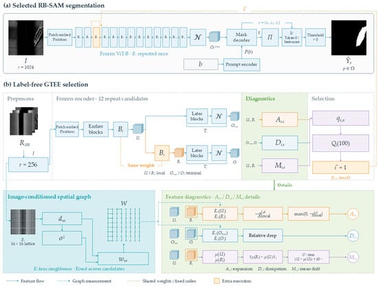
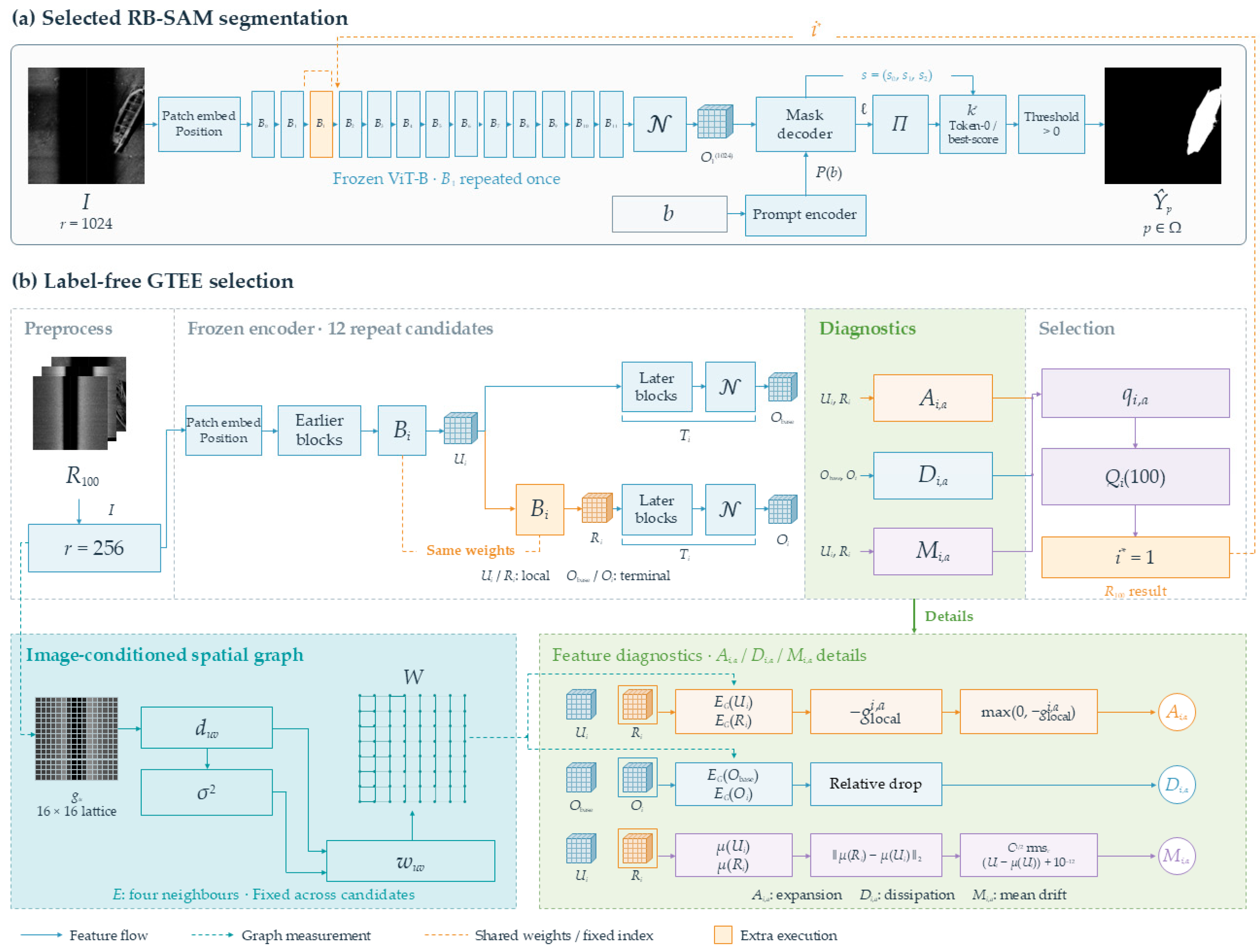
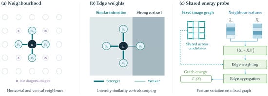
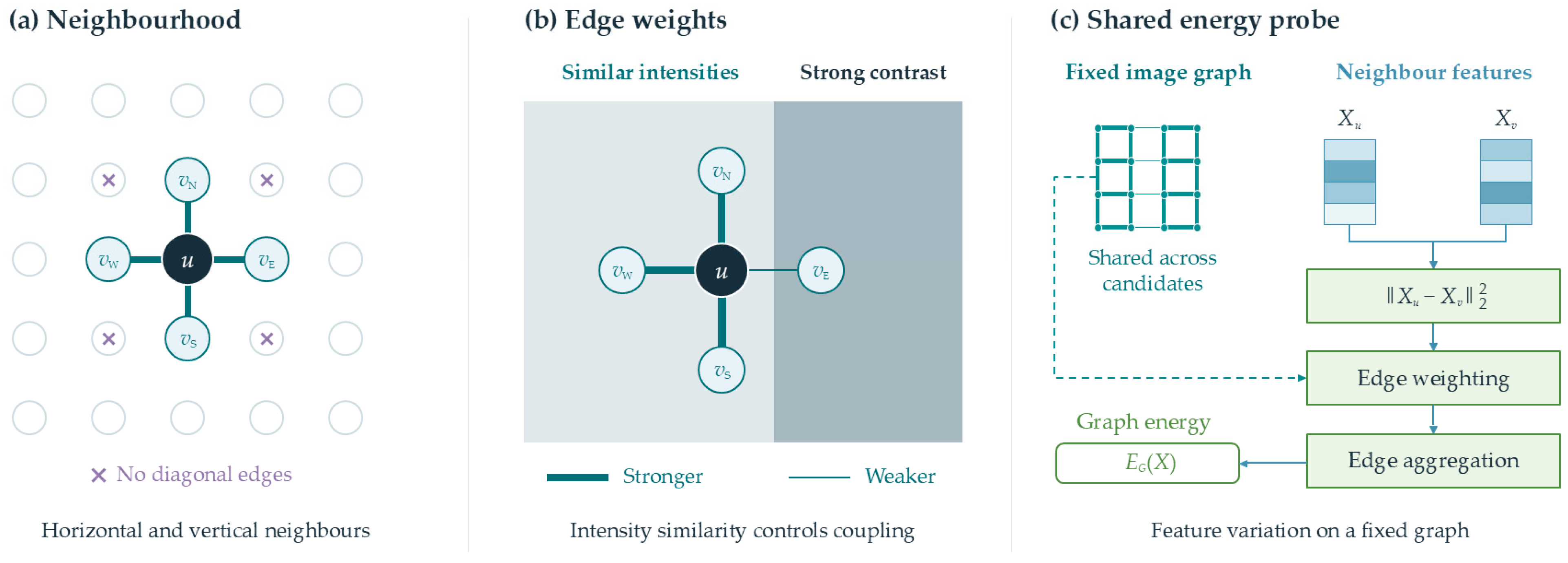
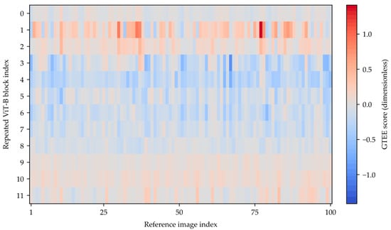
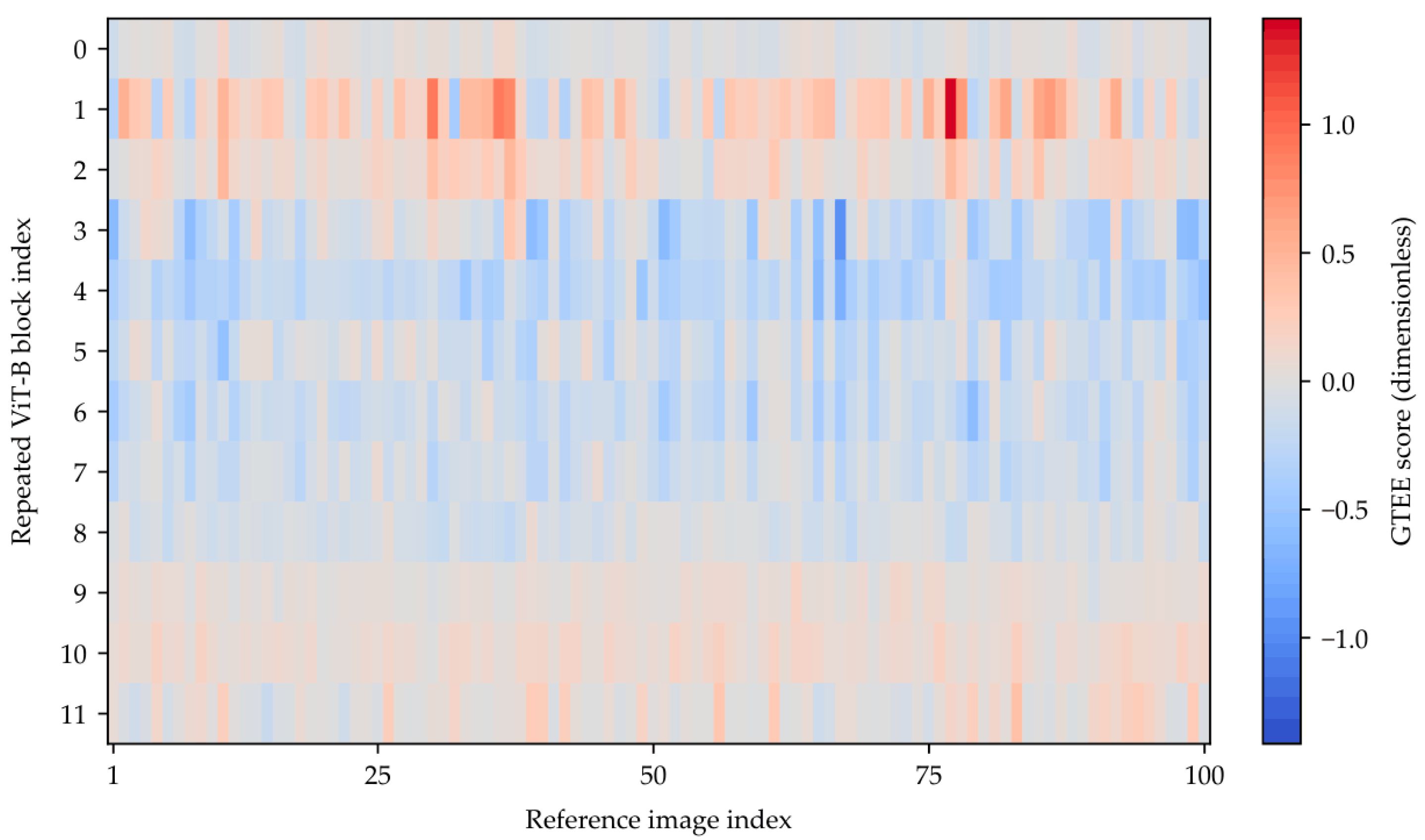
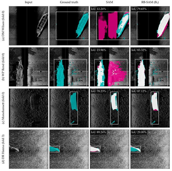
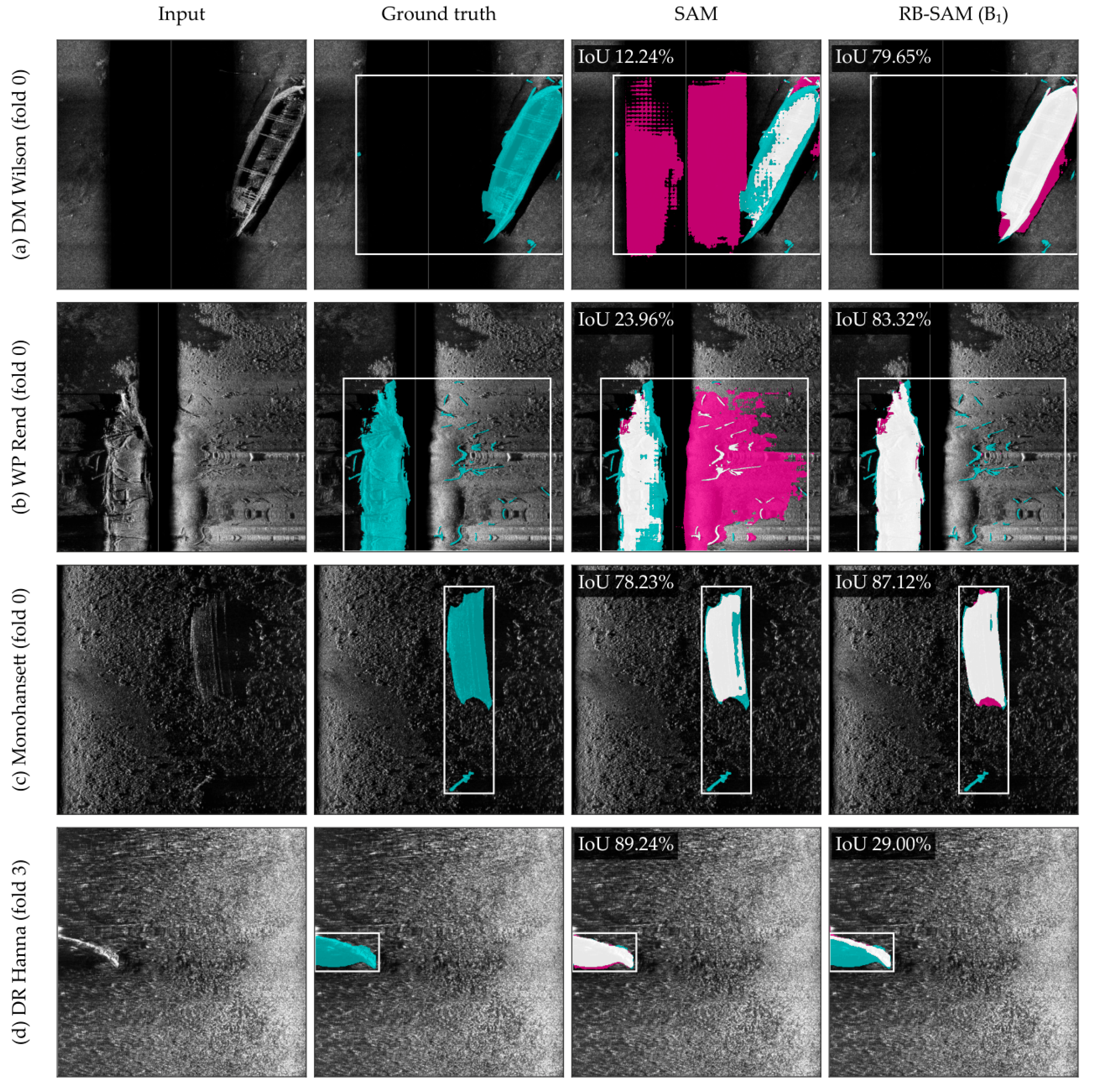
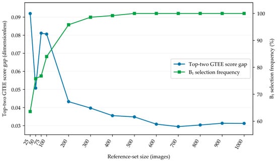

Disclaimer/Publisher’s Note: The statements, opinions and data contained in all publications are solely those of the individual author(s) and contributor(s) and not of MDPI and/or the editor(s). MDPI and/or the editor(s) disclaim responsibility for any injury to people or property resulting from any ideas, methods, instructions or products referred to in the content. |
© 2026 by the authors. Licensee MDPI, Basel, Switzerland. This article is an open access article distributed under the terms and conditions of the Creative Commons Attribution (CC BY) license.