


Abstract
Koopman model predictive control (MPC) iterates a lifted linear predictor over a horizon of tens of samples. Extended dynamic mode decomposition with control (EDMDc), however, fits that predictor by minimising only the one-step residual in the lifted space. This paper bounds the h-step output error of any lifted linear predictor by its one-step residual times an amplification factor that is computable from the model alone. The bound is attained for single-output systems, takes a horizon-uniform form through a scaled Lyapunov certificate, and extends to the suboptimality of the input sequence that MPC selects. The proposed HC-EDMDc minimises the rolled-out output error under a spectral-radius constraint, starts from the closed-form EDMDc solution as a warm start, and is selected by a held-out rolled-out criterion. The evaluation uses four measured benchmarks: a six-axis KUKA KR300 industrial robot, an electro-mechanical positioning system, a cascaded-tank process and the Silverbox oscillator. The one-step estimator returns a non-Schur transition matrix on 8 of 20 fits across 3 records, and its free run leaves the data range; the constraint removes this failure for at most 8.4 % of twenty-step accuracy. HC-EDMDc improves long-horizon accuracy on 2 records, reducing the twenty-step NRMSE on the cascaded tanks from 0.3431 for EDMDc + SR to 0.2827, and returns its warm start on the other 2; the size of the one-step residual does not predict which case a record falls into. Minimising collapses the predictor towards a mean-reverting model on 3 of the 4 records, and the certified bound moves opposite to the realised error on 2 of them. A valid bound is therefore not a model-selection criterion.
Keywords:
Koopman operator; extended dynamic mode decomposition; model predictive control; system identification; prediction horizon; transient amplification; industrial robot; data-driven control MSC:
93B30; 93B45; 47B33
1. Introduction
Model predictive control (MPC) is the standard method for driving constrained multivariable machinery, from industrial manipulators to process units, because it recasts a control specification as an optimisation problem solved online [1,2]. On embedded hardware, its appeal rests on one structural property. When the prediction model is linear, the optimisation is a convex quadratic program (QP), and modern operator-splitting solvers dispatch such problems in microseconds [3]. Nonlinear plants therefore set fidelity against tractability, and much of the data-driven control literature is devoted to reconciling the two.
The Koopman operator offers one reconciliation. Rather than linearising the dynamics around an operating point, it lifts the state into a space of observables in which the evolution is linear but infinite dimensional [4,5,6,7]. Dynamic mode decomposition made this operator accessible from data by extracting modes directly from snapshot sequences [8], and its connection to the Koopman spectrum was established shortly afterwards [9]. Extended dynamic mode decomposition (EDMD) approximates the operator on a finite dictionary by least squares [10,11]. Its convergence to the Koopman operator as the dictionary and the sample count grow is understood [12,13,14], spectral and stability-analytic uses of the operator are well developed [15,16], and finite-data error bounds are now available [17,18,19]. How to choose or learn the dictionary remains an active question [20,21,22,23], and Koopman autoencoders learn the observables jointly with the linear dynamics, often under multi-step or consistency losses [24,25,26].
Embedding the resulting linear predictor in MPC yields Koopman MPC [27]. The scheme has been applied to fluid systems [28], soft manipulators [29] and robotic platforms [30,31], extended to robust and tube-based formulations [32,33,34], and equipped with closed-loop stability guarantees under explicit error bounds [35,36,37]. Bilinear lifted forms retain more of the input dependence at the price of a non-convex control problem and constitute a parallel line of work [38,39,40].
Data-driven and machine-learning methods now extend well beyond control, spanning structural health monitoring and civil infrastructure [41,42,43,44,45,46], graph representation learning and network topology identification [47,48,49,50,51], antenna and electromagnetic design [52,53,54], energy and battery management systems [55,56,57,58], image reconstruction and remote sensing [59,60], fire-risk prediction [61,62], biomedical therapeutics [63], enterprise and social analytics [64,65,66], financial risk management [67], and natural-language processing [68]. In the control domain that the present work occupies, a different route to the same goal dispenses with an identified model altogether. Behavioural methods predict directly from raw trajectory libraries [69,70,71]. Adaptive dynamic programming and reinforcement-learning methods learn the control law or value function from data. Event-triggered adaptive dynamic programming with a dynamic penalty factor handles input saturation with uniformly ultimately bounded closed loops [72], and event-triggering conditions derived from the Hamilton–Jacobi–Bellman solution come with a performance upper bound and a minimum inter-event time [73]. Extended disturbance and state observers support event-triggered data-driven control of networked and disturbed nonlinear systems [74,75], a pseudo-partial-derivative description of the input–output map yields a Q-learning control law with an event-triggering rule [76], and off-policy interleaved Q-learning obtains optimal controllers for unknown affine nonlinear systems from measured trajectories alone [77]. These methods do not iterate a predictive model, which suits online adaptation and communication-limited settings. The present paper concerns the other, model-based branch, in which a lifted linear predictor is identified first and then embedded in MPC. Only this branch provides the QP structure, constraint handling and a state-space model that can be simulated, and it is in this branch that the mismatch between one-step fitting and multi-step use arises.
However, the predictor is fitted in one way and used in another. EDMD with control (EDMDc) minimises a one-step residual in the lifted space, whereas MPC propagates the model over a horizon of tens of samples, so the relevant quantity is the accuracy of the h-step map for h up to the horizon. Composing an approximate operator with itself amplifies its residual. The amplification is governed by the transient behaviour of the lifted transition matrix rather than by its spectral radius, a distinction that is classical for non-normal matrices [78] and that, as shown below, dominates the practical behaviour of Koopman predictors on real records. Recent work reaches the same diagnosis from the estimation side and learns the condensed multi-step map directly, which restores convexity at the price of horizon-specific matrices [79].
To address these gaps, this paper approaches the problem from the opposite direction. It keeps the single recursive linear predictor, which is what makes free-run simulation, spectral analysis and state-space stability certificates available, and asks what has to change in the estimator. The study combines an analysis of how the one-step residual propagates over the horizon, an estimator built on that analysis, a bound that carries model error into the closed loop, and an evaluation on measured data. The contributions are as follows.
- (i)
- An error-amplification analysis (Section 3) bounds the h-step output error of any lifted linear predictor by the product of its one-step residual and the amplification factor , which is computed directly from . A Lyapunov certificate gives a horizon-uniform version of the bound, and a construction shows that the bound is attained in the single-output case. Whereas existing finite-data error bounds [17,18] express the compounded error through spectral or Lipschitz-type constants, is a diagnostic of a single identified model and explains quantitatively why a predictor with an almost vanishing one-step residual can be useless over an MPC horizon.
- (ii)
- A stability-constrained horizon-consistent estimator, HC-EDMDc (Section 4), minimises the rolled-out output error over the horizon subject to a Schur constraint enforced by a spectral-radius retraction. It is warm-started at the closed-form EDMDc solution and selected on a held-out rolled-out criterion, so by construction, it is never worse than its warm start on that criterion (Proposition 3). At , it reduces to a convex one-step output-error problem that differs from EDMDc by the readout projection (Proposition 4). Unlike the horizon-specific condensed maps of [79], HC-EDMDc retains a single recursive predictor that can be simulated indefinitely, carries a spectral-radius certificate, and has a parameter count independent of H. Compared with the multi-step and consistency losses of Koopman autoencoders [24,25,26], it adds the spectral-radius constraint and the held-out selection rule.
- (iii)
- A negative result shows that a valid bound is not automatically a model-selection criterion. The bound of Theorem 1 is valid and worst-case tight, yet along a regularisation path its value is negatively correlated with the realised horizon error on two of the four benchmarks, uncorrelated on a third and positively correlated on the fourth. Minimising the product , the surrogate an optimiser is naturally handed, collapses the predictor towards a mean-reverting model on the three records on which that optimisation makes any progress at all.
- (iv)
- The methods are evaluated on four measured benchmarks rather than on simulated examples, namely a six-degree-of-freedom KUKA KR300 R2500 industrial robot, an electro-mechanical positioning system, a cascaded-tank process and the Silverbox electronic oscillator. A closed-loop study is carried out on a first-principles positioning-system model identified from the same measurements. The paper reports where the horizon-consistent fit helps, where it is neutral and why, and it also reports the computational cost (Section 8.2) and when the estimator is worth using (Section 8.3). Section 8.4 compares the approach with the related methods discussed above.
No single estimator dominates. The stability constraint prevents the free runs that leave the data range, which the plain one-step estimator produces on two of the four benchmarks, at a cost of up to 8.4% in twenty-step accuracy and considerably more at one step. The horizon-consistent refinement helps materially on the two records where it improves on its closed-form warm start, and is neutral on the other two, where it returns that warm start unchanged. Which regime a record falls into is not predicted by the size of its one-step residual, and Section 7 states this explicitly rather than leaving the reader to infer a rule that the data do not support.
The remainder of this paper is organised as follows. As Figure 1 shows, measured records pass through lifting and closed-form estimation to the amplification analysis, the horizon-consistent estimator, and finally open-loop and closed-loop evaluation. Section 2 fixes notation and recalls EDMDc and Koopman MPC. Section 3 develops the amplification analysis, and Section 4 defines the estimator and states its properties. Section 5 carries the model error into the closed loop. Section 6 describes the benchmarks and the protocol, and Section 7 reports the results. Section 8 discusses what the results show, the computational cost and scalability, when to use the estimator, its relation to the literature, and the limitations of the study (Section 8.5). Section 9 concludes.
Figure 1.
Overview of the proposed framework. Measured records are delay-embedded and lifted by a dictionary. The closed-form EDMDc solution serves as the warm start, and the amplification analysis yields . HC-EDMDc minimises the rolled-out output loss under a spectral-radius retraction and selects, by held-out loss, among candidates that include the warm start. The resulting predictor is used for open-loop evaluation and in Koopman MPC, the latter in a closed-loop study on an identified first-principles plant. Dashed arrows indicate where the analysis informs the design of the estimator.
2. Problem Setting and Preliminaries
2.1. Plant, Data, and Lifted Predictor
We consider a discrete-time plant with input and measured output generated by an unknown dynamical system
whose internal state is not available. The data are one or more finite input–output records collected from the physical device.
Since the state is unmeasured, we work with a delay-embedded surrogate state. Fix delay orders and set
Under the usual observability and genericity conditions, the delay vector (2) is a valid state for the input–output behaviour of (1) [80], and delay coordinates are a standard choice of Koopman observables [81,82].
The Koopman operator associated with (1) acts on observables by composition,
where F denotes the induced map on delay coordinates. It is linear but infinite dimensional, and a finite-dimensional approximation is obtained by restricting it to the span of a dictionary . We use the standard control-oriented form in which the lifted state carries the delay state itself,
with a fixed nonlinear feature map. Two dictionaries are used below: random Fourier features approximating a Gaussian kernel [83], and a random subset of quadratic monomials. The predictor is the linear system
with , and a readout . Because the lifted state contains , whose leading block is , the readout is exactly representable; we obtain it by least squares on the fitting data,
Crucially, once (5) is rolled forward, the lifted state is not re-lifted: the predictor is a genuine linear system, which is exactly the property that makes the downstream control problem a QP.
2.2. EDMD with Control
Given consecutive pairs on a fitting index set with , EDMDc [10,27,84] determines from the regularised one-step problem
whose solution is available in closed form. Writing ,
The residual that (7) controls is the root-mean-square one-step lifted residual
2.3. Koopman MPC
For a prediction horizon , weights , , and , and input box constraints , the tracking problem solved at each sampling instant is
Eliminating the lifted states gives the condensed prediction
so that (10) becomes the box-constrained QP
with , , , and D the first-difference matrix on U; the implementation uses a scalar S. Equation (11) makes the object of interest explicit: the controller consumes the powers and the Markov parameters for , not the one-step map.
3. Error Amplification over the Prediction Horizon
This section makes precise what the estimator (7) does and does not control. Let denote the lifted states actually generated by the plant data and define the one-step lifted residuals
so that in (9) is the root-mean-square norm of over the fitting set. We also allow for a readout mismatch , which is zero up to numerical precision for the lift (4) because is a linear function of .
Definition 1 (Amplification factor).
For a predictor and a horizon ,
Theorem 1 (Horizon error bound).
Let be the h-step prediction obtained by rolling (5) forward from with the realised inputs . Then,
and, consequently,
Moreover, let be a set of window starts such that and are defined for every , and let
be the root-mean-square residual over the windows and the root-mean-square readout mismatch at their endpoints. Then, by the Cauchy–Schwarz inequality followed by the triangle inequality in ,
Proof.
Equation (15) follows by induction on h: it holds trivially for by (13), and if it holds for h, then applying (13) once more and collecting terms gives the statement for . The rolled-out prediction is , so subtracting and multiplying by C,
The triangle inequality and submultiplicativity give (16). For (18), apply the Cauchy–Schwarz inequality to (19) in the form , average over to obtain , take square roots, and add the endpoint mismatch with the triangle inequality in . □
The averaged form is stated over the windows rather than over the fitting index set, because the residuals entering an h-step window need not all lie in the set on which of (9) is computed. The two statistics differ even when they do. Consecutive windows overlap, so a residual in the interior of is counted once for each of the h windows that contain it while one near either end is counted fewer times, which makes an overlap-weighted root-mean-square rather than the uniform one of (9). On the records used here, the ratio stays within two percent of unity, but is the statistic the argument requires and Section 7.2 evaluates the certificate with it.
Theorem 1 separates two independent quantities. The estimator (7) minimises ; nothing in it constrains . The next two results show that the second factor is neither a technicality nor conservative.
Proposition 1 (Worst case over residual sequences).
Fix A, C and h, and consider residual sequences with . The worst-case residual contribution to the h-step output error equals
For a single-output system (), one has , so in that case, the residual term of (16) is attained; for , the worst case is , which may be strictly smaller than . The readout term of (16) is attained only if it is aligned with the residual contribution, so (16) as a whole is attained when , which is the case for the lift (4) up to numerical precision.
Proof.
Because the residuals are unconstrained relative to one another, the supremum decouples once a direction w of the output error is fixed: for fixed w, the largest achievable value of is , attained at when that vector is non-zero and at an arbitrary admissible otherwise, since such a term contributes nothing. Maximising over gives (20); the inequality follows from . If , then is a row vector, , and for every i. □
Corollary 1 (Horizon-uniform certificate).
Let . The scaled discrete Lyapunov equation
has a unique solution , and with , ,
Proof.
Two consequences are worth stating explicitly, because both are visible in the experiments of Section 7. First, alone does not keep small: the constant M in (22) is a norm-equivalence factor between the Euclidean and the P-weighted norms. It equals one exactly when is normal in that inner product and grows with the departure from normality, but it also grows when the modal decay rates are widely spread or when is taken close to , so it is not a pure measure of non-normality. Either way, it can be arbitrarily large, which is the discrete-time face of transient growth in non-normal systems [78]. Second, does not by itself make diverge—if the unstable modes are unobservable through C, as for with , the sum (14) stays bounded—but it removes any horizon-uniform certificate, and whenever an unstable mode is observable, the sum grows geometrically in h. The retraction of Section 4 constrains , which is sufficient for a horizon-uniform bound and not necessary; we use it because it is the cheap and structure-agnostic choice, and because a free-run simulation of an unconstrained fit does leave the data range on two of our benchmarks.
Setting in the experiments is compatible with the hypothesis of Corollary 1 in the following sense. Theorem 1 holds for any A and any finite h, so with , it still provides a finite-horizon bound on every horizon used. The spectral-radius retraction returns a matrix with . Where the spectral radius is strictly below one, as for most of the fitted models in Section 7, any satisfies the hypothesis of Corollary 1 and the horizon-uniform certificate applies. A fit that the retraction places exactly on the unit circle keeps the finite-horizon bound but has no horizon-uniform certificate. Section 7.4 reports the results for , values at which the corollary applies directly, and the free-run simulation errors for and differ by at most . Taking in the main experiments therefore leaves the comparison between estimators unchanged.
The last result of this section explains why minimising a one-step criterion is not merely uninformative about but actively biased, and it does so in a form that the noise experiment of Section 7 can test.
Proposition 2 (Attenuation bias of the one-step criterion).
Let y be the stationary first-order autoregression with and e zero-mean, i.i.d., of variance , so that . Let the measurements be with zero-mean, i.i.d., independent of y and of e, of variance , and write . Let be the population minimiser of the H-step criterion and let be the corresponding per-step rate. Then,
Proof.
The criterion is quadratic in with minimiser . Independence of v from y gives and , so . Since and , and is the unique positive root. Monotonicity in H follows because increases to 1. □
The restriction to keeps the per-step rate well defined: for and even H, the H-step criterion determines only , and is defined up to sign.
Proposition 2 is the familiar equation-error versus output-error distinction of system identification [85,86] in a form tied to the horizon: the one-step criterion shrinks the identified dynamics towards zero by a factor that a horizon-H criterion reduces to its H-th root. Read as a prediction about identification from noisy records, it suggests that a horizon-consistent fit should matter more as the output noise grows and less as the fit becomes exact. Section 7 tests that reading on the four benchmarks and does not confirm it; the proposition itself is a population statement about a scalar autoregression and is verified as such. Every statement of this section was checked against a brute-force computation before being written down, using the script code/verify_theory.py in the Supplementary Materials. The two sides of (15), computed once with explicit matrix powers and once by stepwise roll-out, differ by at most in absolute value, and the inequalities were checked instance by instance on randomly generated examples, where (16) held on all 400 instances with a largest ratio of between the actual error and , (18) held with a largest ratio of between its two sides, and the ratio of Corollary 1 never exceeded . For Proposition 1, the analytic worst-case sequence attains to a relative difference of , whereas a direct search over 24,000 random residual sequences reaches at most of and never exceeds it (with several outputs, and the analytic sequence attains ), and the rate of Proposition 2 agrees with Monte Carlo simulation to within for and .
4. Stability-Constrained Horizon-Consistent Estimation
4.1. The Estimator
Theorem 1 suggests two modifications of (7): replace the one-step residual by the quantity the controller actually incurs, and keep under control uniformly in h, which by Corollary 1 follows from a Schur constraint. Let collect the indices t for which the whole window lies inside one contiguous record, and let with be horizon weights. Define the rolled-out output loss
and the (non-convex) stability set
The proposed estimator, HC-EDMDc, is
approached numerically from the closed-form warm start (8). Three implementation elements matter and are stated explicitly so that the reported results are reproducible.
Rolled-out gradient. The map makes (24) a polynomial of degree H in A, so (26) is non-convex for ; we evaluate by propagating the predictor forward inside each window—never re-lifting—and differentiate through that recursion. Writing for the h-step iterate and , back-substitution gives
Feasibility restoration. is not convex and the Euclidean projection onto it has no closed form. We use the scaling retraction
which is exact on the boundary, leaves feasible iterates untouched, and preserves the eigenvector structure of A while scaling its spectrum. It is a feasibility restoration, not a projection: is in general not the closest feasible matrix to A. Constraining instead would be convex but is far too strong here, since a delay-embedded predictor is strongly non-normal and routinely has .
Model selection. The ridge parameter and the stopping iterate are selected on a held-out slice of the training record, using the data term of (24) evaluated on that slice—the penalty is a fitting device and is not part of the validation criterion. The warm start is included among the candidates, and the retraction (28) is applied to every candidate before it is scored, so the model that is returned is the model whose validation loss was measured.
4.2. Properties
Proposition 3 (No degradation relative to the warm start).
Proof.
Immediate from and the definition of the selection rule; feasibility holds because (28) is applied to every candidate before it is scored. □
Proposition 3 is deliberately modest and close to a tautology. It guarantees only that a selection rule which counts the warm start among its candidates cannot return a model that is worse on the criterion it selects by. Nothing follows for the training loss or the test error, and the experiments report both; on one of the four benchmarks, the two do come apart. The statement is still worth one line, because it rules out a real failure mode of non-convex refinement, namely an optimiser that replaces a good closed-form solution by a worse iterate.
Proposition 4
(Behaviour at ; non-convexity for ). For , (24) reduces to the one-stepoutput-error criterion , which is convex in ; it differs from (7), which measures the residual in the lifted space, by the projection C. The same holds whenever for all . If instead for some , (24) is in general non-convex in A: for , , , , , a single window with and gives , whose second derivative at is , negative for .
Proof.
Four guarantees hold for HC-EDMDc. First, every candidate passes through the spectral-radius retraction (28) before it is scored, so the returned model satisfies . Second, by Proposition 3, it is no worse than the warm start on the held-out loss . Third, (27) is the exact gradient of ; checked against automatic differentiation, the largest absolute discrepancy is for and for . Fourth, for , the problem is convex (Proposition 4). For , is a polynomial of degree H in A and the problem is non-convex, so we claim neither a global minimiser nor convergence to a first-order stationary point or a local minimiser. The retraction is a feasibility restoration rather than a Euclidean projection, and the convergence theory of projected gradient methods therefore does not cover these iterates. Whether the first-order condition at the warm start and a short-horizon refinement actually produce descent is checked on data in Section 8.3. Taken together, these guarantees mean that the returned predictor is always feasible and at least as good as the closed-form solution on the criterion used to select it.
4.3. Why Minimising the Bound Surrogate Is Not the Right Objective
Theorem 1 suggests a cheap proxy for the horizon error: the product of its two ingredients, . We call that product a surrogate rather than a bound throughout, because it is neither of the two certified quantities. The pointwise form (16) pairs with the largest residual in each window; the root-mean-square form (18) pairs the larger constant with the overlap-weighted residual and adds the readout term . The product substitutes the fitting-set root-mean-square for both residual statistics and drops , so it is not an upper bound on the horizon error; the only inequality that holds universally between the two constants is . It is nonetheless the quantity an optimiser is naturally handed, since it is the cheapest expression built from the two factors, and it is tempting to minimise it directly and thereby avoid the rolled-out recursion altogether. We implemented this surrogate-minimising estimator, which we label BR-EDMDc, as
where the two factors need no relative weight—that is the appeal of the criterion—and the small ridge term is retained only for conditioning, with the same as the warm start. The following observation explains what we then measured.
Proposition 5 (The surrogate prefers the trivial predictor).
Let be the best input-only model, its residual, and let be any feasible pair with residual ; assume . The pair is feasible with , and the unregularised criterion of (29) assigns it a strictly smaller value than whenever
Proof.
Compare the two values and of the product and rearrange; the logarithm is increasing. That follows from (14) with , only the term surviving, and . □
Proposition 5 is a pairwise comparison, not a statement that the minimiser of (29) equals : it says that whenever (30) holds—taking for the one-step solution, the estimator one would otherwise have used—the criterion ranks the predictor that ignores the state above it. That is already enough to make the criterion useless for selection, and Section 7 reports what the numerical minimiser actually returns.
Condition (30) is satisfied by a wide margin on every benchmark considered here, because is a modest ratio while is one to two orders of magnitude larger than . The measured consequence is reported in Section 7: on the three records where the optimiser moves away from its warm start, BR-EDMDc drives into single digits and returns predictors whose accuracy is that of a mean-reverting model; on the fourth, it makes no progress at all. We record the result because the temptation to optimise a certificate is a natural one. The bound of Theorem 1 takes the worst case over residual directions—exactly of Proposition 1, which equals for a single output—while the realised error involves the specific residual sequence produced by the data. The gap between the two is what makes the surrogate unusable as a training objective, and Section 7.2 measures it along a regularisation path.
5. From Horizon Error to Control Performance
The estimator of Section 4 targets the horizon prediction error. This section connects that quantity to the quality of the decision the controller makes with it. We keep the statement at the level at which it can be proved without extra assumptions—the suboptimality of the input sequence chosen at one sampling instant—and refer to the literature for the closed-loop stability results that build on error bounds of this type [2,35,37,87].
Fix a sampling instant, a reference and the measured lifted state . For an admissible input sequence , let be the prediction (11) and the response the plant would actually produce. With , and as in (12), and carrying the previously applied input, define the predicted and realised costs
and the prediction gap over the admissible set,
If, in addition, the one-step residuals and the readout mismatch generated by every admissible input sequence obey and uniformly along the window, then Theorem 1 applied horizon by horizon gives the computable bound
That uniformity assumption is strong: the residuals are a property of the plant’s response to counterfactual inputs, and the data only reveal them along the recorded trajectories. The theorem below therefore uses as defined in (32), and (33) should be read as what the analysis yields when such a uniform bound is available.
Theorem 2 (Open-loop suboptimality of the certainty-equivalent input).
Let be the sequence returned by the QP (12) and the sequence a controller with perfect predictions would choose. Then,
Proof.
Collect the three cost contributions of (31) into a single vector,
so that and . The two vectors differ only in their first block; hence, for every , and the reverse triangle inequality gives . Therefore,
where the middle inequality is the optimality of for over , which contains . □
Theorem 2 is what ties the estimator to the controller: the loss incurred by using an approximate predictor is controlled by , which is a weighted horizon prediction error of the same kind that (24) minimises. The two are not the same functional— is a worst case over admissible input sequences with the weights Q, whereas (24) is an empirical average over recorded windows with the weights —but both are controlled by the product of (16), and reducing without controlling , which is what the one-step criterion does, need not reduce either.
Two caveats should be stated plainly. First, (34) is an open-loop, per-instant statement; the recursive-feasibility and stability questions for Koopman MPC require additional structure (terminal ingredients or cost controllability) and are treated in [35,36,37], building on the input-to-state-stability view of inherently robust MPC [88]. Second, as defined in (32) is a supremum over admissible input sequences, so the bound is conservative whenever the realised inputs stay in a small part of ; the experiments in Section 7 therefore report measured closed-loop cost rather than the bound.
6. Experimental Setup
6.1. Benchmarks
All identification experiments use physically measured records released for public benchmarking; no synthetic data enter the identification or the reported prediction results. Table 1 summarises them.
Table 1.
Measured benchmarks used in this study. Every record is a physical measurement released for public benchmarking; no synthetic data enter the identification experiments. Sample counts are after the fixed per-plant decimation described in Section 6.
The industrial robot record is the forward-identification task of the KUKA KR300 R2500 ultra SE benchmark [89]: six measured motor torques drive six measured joint positions, sampled at 10 Hz after the filtering and decimation prescribed by the benchmark. The plant exhibits backlash in every joint, pose-dependent inertia, gravitational and hydraulic loading, and temperature-dependent friction, so it is a genuinely hard multiple-input multiple-output identification problem; the benchmark’s own linear state-space baseline attains a test NRMSE of 1.1173 in simulation mode. The EMPS record is an electro-mechanical positioning system—the prismatic joint of a robot—driven by a measured motor force [90]. The cascaded tanks record is a two-tank liquid-level process with a soft saturation and a hard overflow nonlinearity [91], and the Silverbox record is an electronic realisation of a Duffing oscillator [92,93].
Decimation factors are fixed once per plant from its bandwidth and are identical for every estimator: the robot and the tanks are used as supplied, the EMPS is decimated from 1 kHz to a 100 Hz motion-control rate, and the Silverbox is kept at its full rate because its resonance lies close to the Nyquist frequency of any decimated rate.
6.2. Leakage Control in the Robot Record
The robot benchmark concatenates 33 trajectories, each executed twice. Recovering the segment boundaries from the homing pose shows 66 segments organised in blocks of six, with the second execution of segment i appearing as segment ; the median correlation between an execution and its partner is . A naive contiguous or random split would therefore place near duplicates on both sides of the fit/validation boundary. All robot splits below cut only at multiples of six segments, so both executions of every trajectory stay on the same side.
6.3. Protocol
The lifted state is the delay embedding (2) followed by a dictionary; the delay order and dictionary are selected once per benchmark on the rolled-out validation criterion, from a grid of nine candidates spanning delay orders , no dictionary, random Fourier features with 50–200 components, and 200 random quadratic monomials. Inputs and outputs are standardised with training-set statistics; all reported errors are converted back to physical units.
Model selection uses a rotating validation fold: with folds, seed s holds out the s-th contiguous block of the training record (snapped to trajectory-group boundaries for the robot) and fits on the remainder. This makes the reported spread a genuine measure of sensitivity to the fit/validation split rather than an artefact of a random dictionary draw. The ridge parameter is chosen from a nine-point logarithmic grid on the same rolled-out criterion for every estimator, including the one-step baselines, so the baselines are tuned for exactly the figure of merit on which they are scored.
Figures of merit follow the industrial-robot benchmark [89]. For channel n of a record of length K,
with and the standard deviation and mean of the measured channel; both are averaged over channels. We report two variants. is the h-step-ahead error obtained by re-initialising the predictor at every measured sample and rolling forward h steps—the quantity MPC consumes. is the free-run error over the entire test record from a single initial delay state, which is the benchmark’s own simulation-mode figure of merit. A free run that returns a non-finite value is recorded as diverged; no run reported here did so, and the free-run failures discussed below are finite values that leave the data range by many orders of magnitude.
6.4. Estimators Compared
- EDMDc: The closed-form one-step estimator (8).
- EDMDc + SR: The same estimator followed by the spectral-radius retraction (28) with . The returned matrix satisfies ; how this relates to the condition of Corollary 1 is explained in the remark following that corollary in Section 3, and results for are reported in Section 7.4.
- BR-EDMDc: Minimisation of the bound surrogate (29).
- HC-EDMDc (no SR): The rolled-out objective (24) without the stability constraint, included to separate the two ingredients.
- HC-EDMDc: The proposed estimator (26), with the same stability radius .
- NARX: A feed-forward network on the same delay state, trained either on the one-step or on the rolled-out criterion, as a black-box reference outside the Koopman class. Training a black-box model on a rolled-out criterion is the neural counterpart of output-error identification and has been studied in its own right [94,95,96].
Both constrained estimators therefore use the same stability radius , so any difference between EDMDc + SR and HC-EDMDc comes from the objective rather than from the constraint level.
Setting the dictionary to the identity recovers a linear model in delay coordinates, which is the regression form of classical subspace identification [97]; it is included in the dictionary grid and is selected on two of the four benchmarks.
The rolled-out objective is minimised in double precision with Adam on mini-batches of 2048 windows, started from the closed-form solution (8) and run for at most 150 epochs at a base learning rate of . Three details of the schedule matter for reproducing the numbers. The horizon follows a doubling curriculum, training at before the full horizon, which keeps the early iterates from being dominated by the deepest compositions. Feasibility is restored by the retraction (28) every ten optimiser steps rather than at every step, and once more at the end, so the returned iterate is always feasible. Gradients are norm-clipped at one, the learning rate is halved after twelve epochs without improvement, and training stops early on the held-out rolled-out loss with a patience of forty epochs; the selected epoch is the best one seen on that held-out loss, which is what makes Proposition 3 hold by construction. Experiments run on an NVIDIA RTX 5080 GPU; wall-clock fitting times are reported in Table 2.
Table 2.
Prediction accuracy on the measured test records, mean ± standard deviation over five validation folds. NRMSEh is the h-step-ahead error from every test sample; NRMSEsim is the free-run error over the whole test record. A superscript counts folds whose free run diverged, and “div.” marks a row in which every fold diverged. SR denotes the spectral-radius retraction.
6.5. Closed-Loop Study
No physical hardware was available for this study, so the controllers are evaluated against first-principles plant models whose parameters were identified from the same measured records and whose open-loop fits on the held-out measurements are reported. The EMPS positioning system uses the standard rigid-joint model
whose four parameters are obtained by least squares on the measured torque and the finite-difference velocity and acceleration; on the held-out measured record, it reproduces the position with . The cascaded tanks use the two-state square-root outflow model
with an overflow saturation and the four constants fitted by minimising the open-loop simulation error; it reaches on the held-out record.
The predictors in the loop are fitted only on the measured records and never see data from the simulated plants. Even the zero-mismatch level therefore contains a structural plant–model mismatch between the measured apparatus and its first-principles surrogate, of the size indicated by the open-loop fits above. The 10 and levels move the plant further from the apparatus on which the predictors were based by perturbing its dominant physical constants. On the EMPS, the inertia M and the viscous friction are inflated together. On the tanks, the upper-tank outflow coefficient is raised and the pump gain lowered by the same fraction, and with . Results split by mismatch level are given in Section 7.5.
The two plants play different roles. On the EMPS record, all estimators return the same predictor, so that loop is a consistency check, whereas the tank record is the one on which the predictors genuinely differ. The coarser tank surrogate is a limitation of the second experiment and is discussed in Section 8.5.
The controller is the QP (12) solved with OSQP [3]. Its weights are fixed once on the one-step baseline and held identical for every predictor, so that differences in tracking reflect the predictor rather than retuning. A textbook constant output-disturbance estimator provides offset-free tracking, and the input box constraints are taken from the measured input range. Three reference profiles (square wave, sinusoid, smoothed multi-level set-point sequence), three prediction horizons ( on the EMPS, on the tanks) and the three mismatch levels are combined with three validation folds, giving 81 runs per estimator and plant, 27 at each mismatch level.
7. Results
7.1. Prediction Accuracy
Table 2 and Figure 2 report the test accuracy of the five estimators on the four measured records. Three observations organise the rest of this section.
Figure 2.
Test error as a function of the prediction horizon h, mean over five validation folds with the shaded band showing one standard deviation. Both axes are logarithmic. The curves for BR-EDMDc sit at the level of a mean-reverting predictor on three of the four records.
The one-step estimator is not Schur stable. The closed-form estimator (8) returns on 8 of the 20 fits, spread over 3 of the 4 benchmarks, even though its ridge parameter was selected on a rolled-out criterion. We count individual fits rather than fold-averaged spectral radii because averaging first conceals a record on which only one fold leaves the unit disc. On the two records whose fold-mean radius also exceeds one, the free-run simulation leaves the data range: on the cascaded tanks the free-run NRMSE of EDMDc is against 0.443 once the retraction (28) is applied, and the same comparison on the robot record reads 2.045 against 1.914. The retraction costs one eigendecomposition each time it is applied—once per ridge candidate during selection, and periodically during the rolled-out fit—and it is not free in accuracy. At , it raises the test error by 8.4% on the tanks and 2.4% on the robot; at , where the unconstrained fit comes closest to interpolating the record, it costs 706.2% on the robot and 197.9% on EMPS. On Silverbox, where already holds, it changes nothing. The trade is therefore up to 8.4% of twenty-step accuracy, and much more at , against a free run that otherwise leaves the data range by eight orders of magnitude, and we take it as the default for a predictor that will be rolled out over an MPC horizon—not for one that will only ever be used a step at a time. The ablation HC-EDMDc (no SR) shows that this is not an artefact of the one-step criterion: removing the constraint from the horizon-consistent estimator also produces free runs that leave the numerical range on the robot and Silverbox records.
The horizon-consistent fit helps on two of the four records, and the separator is not the residual. On the cascaded tanks, HC-EDMDc improves the twenty-step error from 0.3431 to 0.2827 and the free-run error from 0.443 to 0.352. On Silverbox, the twenty-step error moves from 0.1027 to 0.0985. On the robot and EMPS records, the refinement returns its warm start: on every fold of those two records, no iterate generated by the optimiser improved on the warm start’s held-out rolled-out loss, so the selection rule of Proposition 3 returned it. That is a statement about the finite set of candidates the optimiser produced under the schedule of Section 6, not a proof that the warm start is a stationary point or a minimiser of (24); we did not test for either.
It is tempting to summarise this as “the refinement helps where the one-step residual is not negligible”, and we did so in an earlier draft, but the data do not support it. The root-mean-square lifted residual of the one-step fit is 1.90 on the robot, 6.29 on EMPS, 2.88 on the tanks and 0.99 on Silverbox: the largest of the four belongs to EMPS, which is one of the two neutral records. is in any case not comparable across these records, since it is measured in the lifted coordinates and those differ in dimension and in output scaling. What separates the regimes here is the observable stated above—whether the refinement generates any candidate that improves on its warm start—and we have not established what determines that in advance. Across the paired fold-by-fold comparison of HC-EDMDc against EDMDc + SR, the proposed estimator is no worse on 19 of 20 pairs at : 9 improvements, 10 exact ties contributed by the two records on which the refinement returns its warm start, and 1 regression. The ties pin the median relative change over all pairs to 0.0%; over the 10 pairs that actually differ, it is 4.4%. At , the same comparison gives 10 improvements, 10 ties and 0 regressions, with a median of 6.1% over the differing pairs. These counts are descriptive and we attach no significance test to them: the folds of a record share one held-out test trajectory and largely overlapping training data, so they are not independent replicates, and pooling absolute NRMSE differences across four records of different difficulty would not be testing a single effect.
Where short horizons pay for long ones. With uniform horizon weights, the rolled-out criterion spreads its attention over , so nothing obliges it to match the one-step estimator at . That trade-off materialises on one of the four records. On Silverbox, the one-step error of HC-EDMDc is 5.1 times that of EDMDc + SR, the two curves cross between and , and beyond the crossing, the rolled-out fit is the more accurate of the two. On the cascaded tanks, no such price is paid: the rolled-out fit is at least as accurate at every horizon tested, included. On the robot and EMPS records, the two estimators coincide. Figure 2 shows all four profiles. For an MPC application, the relevant question is therefore not which estimator is better in general but which horizon the controller uses; Section 7.5 takes that question up directly.
7.2. The Certified Bound Does Not Rank Models
Theorem 1 is a valid bound—we verified it numerically on random instances and it is attained in the worst case for single-output systems—so it is natural to ask whether it can be used to rank models. It cannot, and the reason is instructive.
Which quantity is being ranked matters here, and we distinguish two. The certified root-mean-square bound of (18) is , and we evaluate it as stated: with the window-shifted residual of (17) over the admissible windows, not with the fitting-set residual . The two differ by at most a factor 1.017 on these records, and is at the level of because the readout is exact for the lift (4), but the certificate is stated in terms of and reporting it with would understate it. The bare product that BR-EDMDc minimises in (29) is not a certificate at all: it pairs the smaller constant with a different residual statistic and omits . We therefore report the certified bound in Table 3 and treat as the surrogate it is.
Table 3.
Ridge path with everything else held fixed, mean over three validation folds. The fourth column is the certified root-mean-square bound of Theorem 1, evaluated with the overlap-weighted residual of (17); each entry is the mean of the per-fold bound, not a bound formed from averaged factors. The column before SR is the spectral radius of the closed-form estimate before the retraction is applied.
Figure 3 traces the ridge path: for each benchmark the regularisation parameter is swept over nine decades while everything else is held fixed. Panel (a) shows the trade-off the surrogate is made of. Increasing damps the transition matrix and drives down—by a factor of 7 to 10 depending on the record, to values near —while the one-step residual moves comparatively little over most of the path and then rises at the damped end. The certified bound is consequently not monotone in : it decreases along the path on EMPS and the tanks and turns back upwards on the robot and Silverbox, where a rising overtakes the falling amplification. Panel (b) shows the realised error over the same path, which rises throughout.
Figure 3.
Behaviour along the ridge path, mean over three validation folds; the parameter is swept over nine decades with everything else fixed. (a) One-step residual against amplification factor—the two factors of the surrogate. (b) Certified root-mean-square bound against the realised twenty-step test error, with the log–log correlation along each path. (c) Transient gain profiles on the cascaded-tank record at three values of .
The log–log correlation between the certified bound and the twenty-step test error is strongly negative on 2 of the 4 records (EMPS −0.90, cascaded tanks −0.93), essentially absent on Silverbox (−0.04) and positive on the robot (+0.46). For the surrogate , the picture is more uniformly negative—3 of 4 records, Silverbox reaching −0.92—which is worth stating because it is the surrogate, not the certificate, that an optimiser would be handed. On no record does either quantity rank models the way a selection criterion needs to, and on two of them, ranking by the bound would prefer the model that predicts worst. Table 3 gives the path in full.
This is Proposition 5 seen along a continuum rather than at a single optimum. The bound is worst case over residual directions, and its amplification factor is minimised exactly by the damped models that have no dynamics left to amplify. Panel (c) makes the mechanism visible on the tank record: at , the gain profile stays near unity out to , whereas at , it decays geometrically—small , and a model that has forgotten its input by the time the horizon ends.
One use of does survive. It is the quantity that grows without bound in h once an unstable mode is observable through C, and the raw spectral radius along the ridge path reaches 1.5938 on the robot, 1.0090 on the tanks and 1.3451 on Silverbox at some , so the constraint of Section 4 is doing real work at exactly those settings. It does not explain which records the refinement helps on: the two neutral records carry the two largest warm-start values, on the robot and 20.0 on EMPS, against 18.5 and 14.4 on the two active ones.
Figure 4 makes the consequence concrete on the robot record: the free-run simulation of all six joints over the whole six-minute test trajectory, from a single initial delay state.
Figure 4.
Free-run simulation of the six measured joint positions of the KUKA KR300 test record from a single initial delay state, for the one-step estimator with the stability retraction and for the proposed estimator. Panels (a–f) are joints to .
7.3. Minimising the Surrogate Does Not Work
Section 7.2 showed that neither the certified bound nor its surrogate ranks models along a regularisation path. Optimising the surrogate directly is the same phenomenon taken to its conclusion. On 3 of the 4 records, BR-EDMDc moves away from its warm start and reduces from 14.4–20.0 to 2.0–7.1, exactly as its objective asks, and in doing so destroys the predictor: its twenty-step errors in Table 2 land within a factor of two of a model that predicts the channel mean, whose NRMSE is one by the normalisation used here. This is Proposition 5 in action, and it is worth reporting because minimising a certificate—or, as here, the cheap surrogate standing in for one—is an attractive shortcut that avoids the non-convex rolled-out recursion entirely.
The robot record is the exception, and we report it as one rather than averaging it away. On that record, no iterate of the BR-EDMDc fit improved on its own objective, the best-iterate rule returned the closed-form warm start, and the corresponding row of Table 2 therefore coincides with EDMDc + SR at . That record carries the largest lifted state in the study, . We read the outcome as a failure of that optimisation to make progress on the largest instance, not as evidence that minimising the surrogate is harmless: the ridge path of Section 7.2, which lowers the same quantity by a different route, is anti-correlated with the realised error on two of the other three records.
7.4. Ablations
Table 4 varies the training horizon H. The pattern follows Proposition 2: on the benchmarks where the refinement is active, accuracy at improves as H approaches the evaluation horizon and saturates beyond it, while on the benchmarks where the one-step fit is already near-exact, the choice of H is immaterial.
Table 4.
Effect of the training horizon H on the 20-step test error (mean ± standard deviation over three folds). The last column repeats the free-run error of the H = 20 models for reference.
Table 5 varies the stability radius , and the pattern is more heterogeneous than the constraint’s role would suggest. Tightening from to is not free: on EMPS, the free-run error rises from to and on the tanks from to , because a strict radius damps modes the record actually needs. Relaxing to does not produce a matching collapse either—the tank free run is unchanged to three digits and Silverbox and EMPS are unaffected, since their unconstrained radii already lie below the threshold—and only the robot record degrades, from to . The reading we take from this is narrow: is a feasibility switch rather than a performance knob, and values just below one are the ones that leave the fit alone while still bounding the free run. Note that , used throughout the main experiments, is enough for to be finite at every finite h but not for the horizon-uniform certificate of Corollary 1, which requires ; the rows of this table are the ones for which that certificate applies.
Table 5.
Free-run test error as a function of the stability radius imposed by the retraction (mean ± standard deviation over three folds).
Table 6 and Table 7 were run to test the regime dependence that Proposition 2 suggests, and they do not confirm it. Adding output noise to the training record does not widen the gap in favour of the horizon-consistent fit. On the cascaded tanks—the one record where the refinement is active at every noise level—the twenty-step advantage is largest on the clean record at 14.2% and falls to 1.0–7.8% once noise is added. On Silverbox, an advantage of 4.3% on the clean record disappears as soon as noise is present. On EMPS at the largest noise level tested, a relative standard deviation of 0.1, the gap turns negative at −6.4%: the refined model is worse than its warm start on the test record, which Proposition 3 permits, since the guarantee is on the held-out criterion the model is selected on and not on test error at . The training-size sweep is likewise non-monotone; on Silverbox the advantage grows with record length, from 0.6% at a tenth of the record to 4.3% at the full record, which is the opposite of the predicted direction.
Table 6.
Twenty-step test error when zero-mean Gaussian noise of the stated relative standard deviation is added to the training outputs (mean ± standard deviation over three folds).
Table 7.
Twenty-step test error as a function of the fraction of the training record used (mean ± standard deviation over three folds).
We report this as a failure of the prediction to transfer, not as evidence against Proposition 2 itself: that proposition is a population statement about a scalar autoregression, and it is verified as such against a Monte Carlo simulation in Section 3. Two features of the experiment separate it from that setting. The rolled-out criterion is evaluated on the same noisy outputs that corrupt the one-step criterion, so both objectives degrade together rather than one relative to the other; and the model is selected on a held-out loss computed on that same noisy record, which on Silverbox returns the warm start at every noise level above zero. Establishing the regime boundary that Proposition 2 points to would need a design that separates estimation noise from selection noise, which we did not run. Figure 5 summarises both sweeps together with the per-fold spread of the improvement.
Figure 5.
(a) Per-fold relative improvement of HC-EDMDc over EDMDc + SR at ; violins show the distribution over validation folds and dots the individual folds. (b) Improvement as a function of the relative output-noise standard deviation added to the training record. (c) Improvement as a function of the fraction of the training record used. Values above zero favour the proposed estimator.
Table 8 places the comparison outside the Koopman model class. Two NARX networks with identical architecture, differing only in whether training minimises the one-step or the rolled-out output error, reproduce the same ordering as the two linear estimators, which supports the reading that the effect is a property of the training criterion rather than of the lifted representation. The networks are not uniformly more accurate than the lifted linear predictor at the horizons tested, and they forfeit the QP structure that motivates the Koopman construction in the first place.
Table 8.
Neural black-box reference. The two NARX networks share an architecture and differ only in the training horizon, which isolates the effect of the rolled-out criterion outside the Koopman model class; the proposed estimator is repeated from Table 2 for orientation.
7.5. Closed-Loop Tracking
Table 9 and Figure 6 report the closed-loop study described in Section 6.5. The result is essentially null, and we report it as such.
Table 9.
Closed-loop tracking with the same MPC law and weights, driven by predictors from different estimators. Each row aggregates 81 runs: three reference profiles × three prediction horizons × three plant–model mismatch levels × three validation folds. The plants are first-principles models whose parameters were identified from the same measured records (Section 6.5); no hardware experiment was performed.
Figure 6.
Closed-loop tracking, aggregated over three reference profiles, three plant–model mismatch levels and three validation folds. (a) Identified EMPS plant, on which the three estimators return the same predictor and the three curves coincide; (b) identified tank plant, on which the predictors differ; and (c) QP solve time per sampling instant. The three predictors are offset slightly along the horizontal axis for visibility.
Splitting the runs by plant–model mismatch level, as in Table 10, leaves the picture unchanged. On the EMPS plant, the three predictors coincide at every level, and the tracking error grows with the mismatch, from 0.4304 at 0% to 0.4595 at 20%. On the cascaded tanks, HC-EDMDc gives the lowest mean tracking NRMSE at all three levels, below EDMDc + SR by 1.4%, 0.8% and 0.6% at 0%, 10% and 20% mismatch respectively. Each of these differences is smaller than the standard deviation of the corresponding cell, which covers its 27 runs over three reference profiles, three prediction horizons and three validation folds. The ordering of the predictors therefore does not change with the mismatch level, so the near-zero differences in Table 9 are not produced by averaging over levels on which the predictors would separate. No run diverged at any level.
Table 10.
Closed-loop tracking NRMSE split by plant–model mismatch level, mean ± standard deviation over the 27 runs in each cell (three reference profiles × three prediction horizons × three validation folds). The mismatch levels are defined in Section 6.5; the runs are those of Table 9, regrouped.
On the EMPS plant the three estimators return numerically identical predictors—this is the interpolating regime of Section 7—so the three loops coincide to four decimal places. That is the expected consistency check rather than a finding. On the tank plant, where the predictors differ by roughly a fifth in twenty-step open-loop error, the mean closed-loop tracking cost differs between them by 1.0%, and the ordering is not consistent across the three horizons: the proposed estimator is better by 3.6% at and worse by 0.2% at . The mean tracking NRMSE exceeds unity on the tank plant for every controller (1.453 and 1.439), which says plainly that at a twenty-step open-loop error of 0.2827–0.3431, no predictor in this comparison is accurate enough for the horizon the controller uses.
The mechanism behind the compression is worth naming, because it qualifies Theorem 2. The bound there is per-instant and open-loop; in closed loop, the state is re-measured and the disturbance estimate re-anchored at every sample, so only the first few steps of each prediction are ever acted upon, and errors at are largely discarded before they matter. Feedback therefore attenuates exactly the quantity the horizon-consistent objective improves. The practical reading is that open-loop horizon accuracy is a necessary but far from sufficient proxy for closed-loop benefit, and that a closed-loop study should not be presented as a corollary of an open-loop one.
The QP itself is never the bottleneck: over every closed-loop run, the mean solve time stays below 0.42 ms and the 95th percentile reaches 1.00 ms at the longest horizon tested, , on a lifted state of a few hundred dimensions, so the entire cost of the method sits in the offline fit reported in Table 2.
8. Discussion
8.1. What the Results Say
The experiments support a narrower claim than “horizon-consistent training improves Koopman predictors”. They support the statement that the horizon error of a lifted linear predictor factorises, in the sense of Theorem 1, into a residual and an amplification, and that the two factors have to be managed separately.
The amplification factor is the part that is cheap to control and expensive to ignore. Requiring costs one eigendecomposition per retraction and, on the records where the constraint binds, up to 8.4% of twenty-step accuracy—considerably more at —and it is the difference between a predictor that can be simulated over a six-minute record and one that cannot. It is not needed for Theorem 1 itself, which is a finite-horizon statement and holds for every A; a strict radius buys the horizon-uniform certificate of Corollary 1, which requires and therefore does not apply at the used in the main experiments. That said, certifies very little on its own: the measured transient gains in Figure 3c grow by orders of magnitude before they decay, and Corollary 1 shows why—the constant M is a condition number of the Lyapunov solution, not a spectral quantity.
The residual is the part we understand less well. Proposition 2 offers a candidate mechanism. The one-step criterion shrinks the identified dynamics by a factor , where is the noise-to-signal ratio in the regressors, and a horizon-H criterion reduces that to its H-th root, so a rolled-out fit should matter more where the one-step fit is less exact. On these four records, that reading does not survive contact with the data. The record with the largest lifted residual is EMPS, and it is one of the two on which the refinement changes nothing; and deliberately degrading the records with output noise, which by the same argument should enlarge the effect, shrank it instead (Section 7). A narrower and more mechanical observable separates the records. On the two neutral records, the optimiser generated no candidate that improved on its closed-form warm start, so the selection returned it. The warm start is not a first-order stationary point there, yet no epoch of the fit lowers either the training objective or the held-out loss, and Section 8.3 shows that this is visible within the first twenty epochs. Reporting both regimes rather than the favourable one is, we think, the useful contribution. It tells a practitioner to read the opening epochs of the fit before paying for the whole non-convex optimisation, and it marks where our own explanation stops being predictive, since the residual does not say in advance which regime a record falls into.
The negative result on the bound deserves emphasis, because it cuts against the way such bounds are often used. Theorem 1 is valid and, by Proposition 1, attained in the worst case; nevertheless, along a regularisation path, its value is strongly negatively correlated with the realised horizon error on 2 of the four records, uncorrelated on a third and positively correlated only on the fourth, and minimising the surrogate that an optimiser would actually be handed drives the estimator to a nearly trivial model on 3 of them. The reason is structural rather than a matter of constants: the amplification factor is minimised by damped models, and damping is precisely how a predictor stops being useful. A valid bound is not automatically a valid model-selection criterion, and reporting a small certified error can mean the model has been flattened rather than improved. A related point has been made from a different direction for uncontrolled EDMD, namely that the one-step residual is not the quantity that measures predictive quality and that consistency-based diagnostics track it better [98].
The size of the certificate on the measured records makes the same point in absolute terms. On the warm-start models (EDMDc + SR with the ridge parameter selected by the original protocol, , ), evaluated on the fitting windows in standardised units and averaged over five folds, the certified root-mean-square bound of (18) is 41.1 on the industrial robot against a realised twenty-step RMS error of 0.083, 126 against 0.0050 on EMPS, 54.5 against 0.23 on the cascaded tanks and 14.5 against 0.093 on Silverbox. The ratio of realised error to bound lies between and , and , and , and and on the four records, so the certificate exceeds the error by between two and four and a half orders of magnitude. On random instances, the same ratio reaches 0.41 for (18) and 0.64 for (16), and Proposition 1 attains equality for a single output. The bound is therefore tight in the worst-case sense and numerically large on measured data, because the realised residual sequences are far from aligned with the worst-case directions. The factorisation of Theorem 1 does provide an explanation of where the horizon error comes from, in particular of why an unstable mode that is observable through C is fatal while is not by itself reassuring, together with the guarantee that the error stays finite over every finite horizon. It is not a numerical forecast of that error. The constant of Theorem 2 is to be read in the same way, which is why the closed-loop part of this study reports measured cost (Section 7.5) rather than the bound.
8.2. Computational Cost and Scalability
The cost of the horizon-consistent fit is set by the rolled-out recursion. One epoch propagates every window through H steps, and each step multiplies the lifted state by an matrix and the input by an matrix and applies one readout, so the forward and backward passes together cost per epoch. The automatic-differentiation graph holds entries for a batch of b windows, and the spectral-radius retraction adds one eigendecomposition every ten steps. The closed-form EDMDc estimate costs and is computed once. On the four records, this difference appears in the column of Table 2, where the fit time rises from 0.6 s for EDMDc to 28.4 s for HC-EDMDc on the robot, from 0.4 s to 4.4 s on EMPS, from below 0.1 s to 1.2 s on the tanks and from 0.1 s to 27.3 s on Silverbox.
Table 11 separates the three factors of the per-epoch cost on the Silverbox record, varying the lifted dimension N, the training horizon H and the number of training windows one at a time.
Table 11.
Training time per epoch of the horizon-consistent fit on the Silverbox record, measured on an RTX 5080 GPU in double precision with a batch size of 2048; each entry is the mean over ten timed epochs, without the horizon curriculum. The last column is the time of one closed-form EDMDc fit at the same lifted dimension. The three blocks vary the lifted dimension N, the training horizon H and the number of training windows (10, 25, 50 and 100% of the training record) in turn.
The time per epoch is close to linear in the training horizon and in the number of windows, rising from 0.55 s at to 8.30 s at and from 0.23 s at 5185 windows to 1.81 s at 52,030. The dependence on N is flatter than the complexity count suggests at small sizes. Up to , the GPU is not saturated and the time stays between 1.68 s and 2.02 s, whereas from to , it grows from 4.34 s to 13.59 s, about 3.1 times, in line with the term. The closed-form fit stays at or below 1.53 s over the whole range, and the setting , that recurs in all three blocks (1.63–1.81 s) indicates the resolution of these timings.
The online cost of Koopman MPC does not depend on how the predictor was identified. The dimension of the condensed QP is fixed by the prediction horizon and the input dimension m, so every estimator in this study yields a QP of the same size. In the closed-loop runs, the mean solve time stayed below 0.42 ms and the 95th percentile reached 1.00 ms at (Section 7.5), which places the whole additional cost of the method in the offline fit.
The horizon-consistent fit is therefore suited to applications in which the model is identified once offline and then used over many control periods. There, an offline cost of a few seconds to a few tens of seconds is an acceptable price for long-horizon accuracy or a stable free-run simulation. Adaptive schemes that re-identify the model at every sampling period are better served by the closed-form EDMDc estimate or its recursive form.
8.3. When to Use the Horizon-Consistent Fit
The results of Section 7, together with a short probe from the warm start, give a practitioner an ordered sequence of checks. The probe was run on every record and fold. It evaluates the gradient of at the warm start and then runs twenty epochs from it at the original learning rate over the full horizon , recording after each epoch the training rolled-out objective and the held-out loss. The four steps are as follows.
- Fit the closed-form EDMDc estimate first and check . The one-step estimator returned on 8 of the 20 fits in this study, and whenever the radius is not below one, the spectral-radius retraction should be applied. Its price is at most 8.4% of twenty-step accuracy, against a free run that otherwise leaves the data range.
- Establish which part of the horizon the controller actually uses. A controller that relies on one-step or very short predictions is better served by EDMDc + SR, since on Silverbox the one-step error of HC-EDMDc is 5.1 times that of EDMDc + SR and the two curves cross only between and . For long horizons, HC-EDMDc is the appropriate choice, with the training horizon matched to the control horizon, because Table 4 shows the accuracy at improving as H approaches the evaluation horizon. On the cascaded tanks the rolled-out fit is no worse at any horizon tested.
- Read the first twenty epochs of the fit. The gradient at the warm start is non-zero on every record and fold, with the scale-free first-order measure between and , so the warm start is never a first-order stationary point. Even so, on the robot and EMPS records, no epoch-end iterate lowered the training objective or the held-out loss on any of the five folds, and the held-out criterion returns the warm start. Both warm starts nearly interpolate their records, with NRMSEh+=5 of 0.0008 and 0.0013 against 0.1332 on the tanks and 0.0314 on Silverbox, and a first-order method finds no descent step from them. On the cascaded tanks the training objective fell on four of five folds, by 10.5–41.7%, while the held-out loss fell on two folds (17.3% and 45.3%) and rose on two (57.3% and 112.8%). That record is short, and selection on the held-out set decides the outcome. On Silverbox, the training objective fell on all five folds by 5.5–8.6% and the held-out loss by 5.2–8.4%, which is the regime in which the refinement pays. The probe took 2.5 s on EMPS, 2.0 s on the tanks, 17.1 s on the robot and 39.0 s on Silverbox.
- Do not decide on the size of the one-step residual or of the certified bound. The residual is 1.90 on the robot, 6.29 on EMPS, 2.88 on the tanks and 0.99 on Silverbox, and the largest of the four belongs to EMPS, on which the refinement changes nothing. The bound does not rank models either (Section 7.2).
These checks distinguish three regimes, namely a warm start from which no descent step is found, a short record on which held-out selection dominates, and a record on which training and held-out losses fall together. They turn a boundary that could previously be observed only after the full fit into a quantity that can be read once the fit has started.
8.4. Relation to the Literature
Earlier work has already observed that composing an EDMD approximant amplifies its error. This observation motivates the finite-data error bounds of [17,18] and the closed-loop guarantees built on them [35,37], and it is the explicit starting point of the multi-step formulation of [79].
Our treatment differs from these works in two respects. First, we express the amplification through the computable quantity rather than through a spectral or Lipschitz surrogate, which makes it available as a per-model diagnostic and shows, via Proposition 1, that it is attained for single-output systems. Second, and in deliberate contrast to [79], we keep a single recursive lifted linear predictor rather than learning horizon-dependent condensed maps. This choice gives up convexity, the strength of their formulation, and in return provides a model that can be simulated beyond its training horizon, a spectral-radius certificate, and a parameter count independent of H. Which trade is preferable depends on whether the model is wanted as a one-shot horizon predictor or as a state-space object.
Neither ingredient of the proposed estimator is new on its own. Training on a rolled-out criterion is what separates output-error identification from equation-error methods [85,86], and it appears in the learning literature as multi-step or consistency losses for Koopman autoencoders [24,25,26]. Stability-constrained learning of linear dynamics has a similar history [99,100,101,102]. Recent work parametrises Koopman models with built-in stability and stabilisability [103] or learns a noise-robust stable Koopman operator from Hankel-DMD observables for model predictive control [104]. Our contribution is to tie both ingredients to the same computable bound and to measure what each is worth on measured industrial records.
Table 12 places the proposed estimator among five classes of existing approaches. HC-EDMDc is the only row that combines a single recursive predictor, an explicit stability constraint and a computable multi-step error bound. The price is a training problem that is non-convex for every .
Table 12.
Training criterion, predictor structure, stability handling and guarantees of related identification approaches and of the proposed estimator.
The analysis also applies beyond the estimator and plant studied here. Theorem 1, Proposition 1 and Corollary 1 use only the fact that the predictor is applied recursively, so they hold for any lifted linear predictor, including the local predictor of each subsystem in distributed MPC. In Koopman-DMPC under bounded communication delay [105], neighbour information arrives up to d samples late, each local prediction extrapolates steps, and the relevant amplification factor is . HC-EDMDc can then be trained with , with the neighbours’ coupling signals entering B as additional input channels. Bilinear lifted forms [38,39] have a state-dependent input matrix, so the bound has to be re-derived for them. The experiments in this paper cover only centralised MPC of a single plant.
8.5. Limitations
Several limitations remain. First, the closed-loop plant is not hardware but a first-principles plant model identified from the same measured record as the predictor. With an open-loop fit of , the EMPS model is a reasonable stand-in. The cascaded-tanks model is considerably coarser (), so the absolute tracking levels obtained on it do not indicate attainable performance. On that record, only the comparison between predictors run against the identical plant carries meaning, and that comparison differed by less than one percent. A hardware loop, or a plant identified from records held out from predictor training, is needed before the closed-loop numbers can be read as more than relative.
Second, the closed-loop study does not separate the estimators, and no setting has been constructed in which it would. An open-loop gain of roughly one fifth at changed closed-loop cost by 1.0%. The reason is structural and is given in Section 7.5. Receding-horizon feedback discards most of each prediction. A closed-loop benefit from horizon-consistent identification can only be shown in a regime that forces the loop to rely on the far end of its prediction, such as long sampling intervals, input-rate limits or explicitly economic objectives, and that experiment remains to be done.
Third, the rolled-out objective (24) is non-convex. It is solved by a first-order method under a horizon curriculum, starting from a closed-form warm start. Proposition 3 guarantees only that the returned model does not worsen the criterion on which it is selected. No guarantee of reaching a global minimiser is available, and on the two benchmarks where no generated iterate improved on the warm start, the optimiser made no progress.
Fourth, the retraction (28) restores feasibility without being the Euclidean projection onto . The iterates therefore fall outside the convergence theory of projected gradient methods.
Fifth, the spectral-radius constraint governs asymptotic behaviour only. By Corollary 1, the constant M in is the condition number of the Lyapunov solution and is not bounded by . Imposing consequently neither limits transient amplification nor guarantees better prediction accuracy. In Figure 3c, the gain curves of models that satisfy the constraint grow by several orders of magnitude before decaying, and in Table 5, tightening the radius to raises the EMPS free-run simulation error from 0.088 to 0.664. Criteria that act on transient amplification directly do exist. A spectral-norm or contraction constraint is convex and would restore the projected-gradient theory, but it is far too strong for delay-embedded predictors. A Lyapunov inequality for a given P, or an LMI constraint with an upper bound on , constrains M as well. Stable parametrisations that are stable by construction [102,103,104] and constraint-generation or nearest-stable-matrix methods [99,100,101] offer further routes. Combining these criteria with the rolled-out objective and comparing their accuracy cost has not been done here and is the next step.
Sixth, the evidence comes from four records, and however different they are, four records remain a small sample. Three are single-output. Only the robot record is genuinely multivariable, and the refinement is neutral on it. The regime boundary proposed in Section 7 thus rests on the two records where the refinement is active, and the noise and training-size sweeps designed to probe it did not reproduce the predicted direction. The boundary is a conjecture, and a weaker one than expected. The distributed and delayed setting of Koopman MPC discussed in the preceding subsection was not tested experimentally.
Finally, Theorem 2 is an open-loop suboptimality statement that holds at each instant. A closed-loop guarantee would require terminal ingredients or a cost-controllability assumption of the kind used in [2,35]. The constant in (32) is a supremum over the whole admissible input set, so it is conservative whenever the realised inputs cover only part of that set.
9. Conclusions
This paper quantified the gap between how extended dynamic mode decomposition fits a lifted linear predictor and how model predictive control uses it. The fit minimises a one-step residual, whereas the controller applies the predictor over a horizon of tens of samples. Theorem 1 bounds the h-step output error by the product of the one-step residual and the amplification factor , and Proposition 1 shows that the bound is attained for single-output systems. Corollary 1 gives a horizon-uniform version through a scaled Lyapunov certificate, whose constant is a norm-equivalence factor rather than a spectral one. Theorem 2 carries the same quantity into the control loop and bounds the suboptimality of the certainty-equivalent input sequence by twice the weighted horizon prediction error.
The two ingredients of the resulting estimator, HC-EDMDc, behave differently on four measured industrial records, and both outcomes are worth stating. HC-EDMDc minimises the rolled-out output error under a spectral-radius constraint, starts from the closed-form solution as its warm start and is selected on a held-out rolled-out criterion. The stability constraint prevents the free runs that leave the data range, which the unconstrained one-step estimator produces on two of the four benchmarks, at a cost of at most 8.4% in twenty-step accuracy and considerably more at one step. The horizon-consistent refinement improves horizon accuracy on the two records where it finds an improvement over its warm start—by roughly a fifth on the cascaded-tank record—and returns that warm start unchanged on the other two. The size of the one-step residual does not predict which case a record falls into, since the largest residual of the four belongs to a neutral record. The first twenty epochs of the fit already show the case (Section 8.3); on the robot and EMPS records, no iteration lowers the training objective, on the cascaded tanks, the training objective falls while the held-out loss rises and falls, and on Silverbox, both fall together. Proposition 2 offers a candidate explanation for the boundary through the attenuation bias of the one-step criterion, but the noise and data-size sweeps do not confirm the direction it predicts, and we report them as they came out; the experiments do not identify a quantity that predicts the regime in advance. We also report a negative result. Although the bound of Theorem 1 is valid and worst-case tight, its value moves opposite to the realised horizon error along a regularisation path on 2 of the four records, is absent on a third and runs the other way on the fourth. Minimising the product directly collapses the predictor towards a mean-reverting model on the three records on which that optimisation improves its own objective at all. On the four recorded warm-start models, the certified RMS bound exceeds the realised twenty-step error by two to four and a half orders of magnitude (Section 8). A valid certificate is therefore not automatically a model-selection criterion.
Five directions follow from these results.
- The amplification factor is differentiable and cheap to evaluate, so it can enter the choice of dictionary and delay order rather than serve only as a post hoc diagnostic.
- The boundary between the regimes identified here is empirical. A finite-sample statement relating dictionary richness, sample count and the horizon at which the two criteria separate would allow for the three cases to be predicted before fitting.
- The spectral-radius constraint can be replaced by stability conditions that limit transient amplification directly, such as Lyapunov or LMI constraints with an upper bound on and parametrisations that are stable by construction. Combining these conditions with the rolled-out criterion would show how their accuracy cost compares with that of the spectral-radius constraint.
- The analysis and the estimator can be extended to distributed Koopman MPC and to Koopman MPC with communication delay, where the amplification factor becomes , and to event-triggered data-driven control. In each setting, closed-loop stability and recursive feasibility have to be established under a terminal ingredient or a cost-controllability assumption.
- The closed-loop evaluation here is against an identified first-principles plant. A hardware study on an industrial manipulator, with scenarios that force the controller to rely on the far end of the prediction (long sampling intervals, input-rate limits, economic objectives), would test whether the open-loop gains turn into closed-loop gains.
Supplementary Materials
The following supporting information can be downloaded at: https://www.mdpi.com/article/10.3390/math14214047/s1, Analysis code (data staging, estimators, baselines, Koopman MPC controller, figure generation and numerical checks of the theoretical results) and the per-run result files behind every number and table reported in the article.
Author Contributions
Conceptualization, D.T.; methodology, J.Z. and D.T.; software, J.Z.; validation, J.Z.; formal analysis, J.Z.; investigation, J.Z.; data curation, J.Z.; writing—original draft preparation, J.Z.; writing—review and editing, D.T.; visualization, J.Z.; supervision, D.T.; project administration, D.T. All authors have read and agreed to the published version of the manuscript.
Funding
This research received no external funding.
Data Availability Statement
All four records analysed in this study are publicly released measurement data and no new data were created. The industrial-robot identification benchmark is available from the RPTU Kaiserslautern research-data repository at https://doi.org/10.26204/DATA/5 under a dual MIT/CC BY-SA 4.0 licence (accessed on 11 August 2026). The electro-mechanical positioning system, cascaded-tank and Silverbox records are available from the nonlinear-system-identification benchmark collection at https://www.nonlinearbenchmark.org/benchmarks/emps (accessed on 11 August 2026), https://www.nonlinearbenchmark.org/benchmarks/cascaded-tanks (accessed on 11 August 2026) and https://www.nonlinearbenchmark.org/benchmarks/silverbox (accessed on 11 August 2026). The Supplementary Materials contain the complete analysis code—data staging, estimators, baselines, controller, figures of merit and the numerical checks of the theorems, propositions and corollary—together with the per-run result files behind every number and table reported here. The measured records themselves are not redistributed in them: prepare_data.py stages them from the sources above into the form the remaining scripts consume, after which those scripts reproduce the reported values.
Conflicts of Interest
The authors declare no conflicts of interest.
References
- Rawlings, J.B.; Mayne, D.Q.; Diehl, M.M. Model Predictive Control: Theory, Computation, and Design, 2nd ed.; Nob Hill Publishing: Madison, WI, USA, 2017. [Google Scholar]
- Grüne, L.; Pannek, J. Nonlinear Model Predictive Control: Theory and Algorithms, 2nd ed.; Springer: Cham, Switzerland, 2017. [Google Scholar]
- Stellato, B.; Banjac, G.; Goulart, P.; Bemporad, A.; Boyd, S. OSQP: An operator splitting solver for quadratic programs. Math. Program. Comput. 2020, 12, 637–672. [Google Scholar] [CrossRef] [Scilit]
- Koopman, B.O. Hamiltonian Systems and Transformation in Hilbert Space. Proc. Natl. Acad. Sci. USA 1931, 17, 315–318. [Google Scholar] [CrossRef] [Scilit]
- Mezić, I. Spectral Properties of Dynamical Systems, Model Reduction and Decompositions. Nonlinear Dyn. 2005, 41, 309–325. [Google Scholar] [CrossRef] [Scilit]
- Budišić, M.; Mohr, R.; Mezić, I. Applied Koopmanism. Chaos Interdiscip. J. Nonlinear Sci. 2012, 22, 047510. [Google Scholar] [CrossRef] [Scilit]
- Brunton, S.L.; Budišić, M.; Kaiser, E.; Kutz, J.N. Modern Koopman Theory for Dynamical Systems. SIAM Rev. 2022, 64, 229–340. [Google Scholar] [CrossRef] [Scilit]
- Schmid, P.J. Dynamic mode decomposition of numerical and experimental data. J. Fluid Mech. 2010, 656, 5–28. [Google Scholar] [CrossRef] [Scilit]
- Rowley, C.W.; Mezić, I.; Bagheri, S.; Schlatter, P.; Henningson, D.S. Spectral analysis of nonlinear flows. J. Fluid Mech. 2009, 641, 115–127. [Google Scholar] [CrossRef] [Scilit]
- Williams, M.O.; Kevrekidis, I.G.; Rowley, C.W. A Data–Driven Approximation of the Koopman Operator: Extending Dynamic Mode Decomposition. J. Nonlinear Sci. 2015, 25, 1307–1346. [Google Scholar] [CrossRef] [Scilit]
- Klus, S.; Nüske, F.; Koltai, P.; Wu, H.; Kevrekidis, I.; Schütte, C.; Noé, F. Data-Driven Model Reduction and Transfer Operator Approximation. J. Nonlinear Sci. 2018, 28, 985–1010. [Google Scholar] [CrossRef] [Scilit]
- Korda, M.; Mezić, I. On Convergence of Extended Dynamic Mode Decomposition to the Koopman Operator. J. Nonlinear Sci. 2018, 28, 687–710. [Google Scholar] [CrossRef] [Scilit]
- Mezić, I. On Numerical Approximations of the Koopman Operator. Mathematics 2022, 10, 1180. [Google Scholar] [CrossRef] [Scilit]
- Arbabi, H.; Mezić, I. Ergodic Theory, Dynamic Mode Decomposition, and Computation of Spectral Properties of the Koopman Operator. SIAM J. Appl. Dyn. Syst. 2017, 16, 2096–2126. [Google Scholar] [CrossRef] [Scilit]
- Mauroy, A.; Mezic, I. Global Stability Analysis Using the Eigenfunctions of the Koopman Operator. IEEE Trans. Autom. Control 2016, 61, 3356–3369. [Google Scholar] [CrossRef] [Scilit]
- Mauroy, A. Koopman Operator Framework for Spectral Analysis and Identification of Infinite-Dimensional Systems. Mathematics 2021, 9, 2495. [Google Scholar] [CrossRef] [Scilit]
- Nüske, F.; Peitz, S.; Philipp, F.; Schaller, M.; Worthmann, K. Finite-Data Error Bounds for Koopman-Based Prediction and Control. J. Nonlinear Sci. 2023, 33, 14. [Google Scholar] [CrossRef] [Scilit]
- Philipp, F.M.; Schaller, M.; Worthmann, K.; Peitz, S.; Nüske, F. Error bounds for kernel-based approximations of the Koopman operator. Appl. Comput. Harmon. Anal. 2024, 71, 101657. [Google Scholar] [CrossRef] [Scilit]
- Kostic, V.; Novelli, P.; Maurer, A.; Ciliberto, C.; Rosasco, L.; Pontil, M. Learning Dynamical Systems Via Koopman Operator Regression in Reproducing Kernel Hilbert Spaces. In Proceedings of the Advances in Neural Information Processing Systems 35, New Orleans, LA, USA, 28 November–9 December 2022; pp. 4017–4031. [Google Scholar] [CrossRef] [Scilit]
- Li, Q.; Dietrich, F.; Bollt, E.M.; Kevrekidis, I.G. Extended dynamic mode decomposition with dictionary learning: A data-driven adaptive spectral decomposition of the Koopman operator. Chaos Interdiscip. J. Nonlinear Sci. 2017, 27, 103111. [Google Scholar] [CrossRef] [Scilit]
- Folkestad, C.; Pastor, D.; Mezic, I.; Mohr, R.; Fonoberova, M.; Burdick, J. Extended Dynamic Mode Decomposition with Learned Koopman Eigenfunctions for Prediction and Control. In Proceedings of the 2020 American Control Conference (ACC), Denver, CO, USA, 1–3 July 2020; pp. 3906–3913. [Google Scholar] [CrossRef] [Scilit]
- Korda, M.; Mezic, I. Optimal Construction of Koopman Eigenfunctions for Prediction and Control. IEEE Trans. Autom. Control 2020, 65, 5114–5129. [Google Scholar] [CrossRef] [Scilit]
- Cibulka, V.; Korda, M.; Haniš, T. Dictionary-Free Koopman Model Predictive Control with Nonlinear Input Transformation. SIAM J. Appl. Dyn. Syst. 2025, 24, 94–130. [Google Scholar] [CrossRef] [Scilit]
- Lusch, B.; Kutz, J.N.; Brunton, S.L. Deep learning for universal linear embeddings of nonlinear dynamics. Nat. Commun. 2018, 9, 4950. [Google Scholar] [CrossRef] [Scilit]
- Otto, S.E.; Rowley, C.W. Linearly Recurrent Autoencoder Networks for Learning Dynamics. SIAM J. Appl. Dyn. Syst. 2019, 18, 558–593. [Google Scholar] [CrossRef] [Scilit]
- Azencot, O.; Erichson, N.B.; Lin, V.; Mahoney, M.W. Forecasting Sequential Data Using Consistent Koopman Autoencoders. In Proceedings of the 37th International Conference on Machine Learning; Proceedings of Machine Learning Research: Cambridge, MA, USA, 2020; Volume 119, pp. 475–485. [Google Scholar]
- Korda, M.; Mezić, I. Linear predictors for nonlinear dynamical systems: Koopman operator meets model predictive control. Automatica 2018, 93, 149–160. [Google Scholar] [CrossRef] [Scilit]
- Arbabi, H.; Korda, M.; Mezic, I. A Data-Driven Koopman Model Predictive Control Framework for Nonlinear Partial Differential Equations. In Proceedings of the 2018 IEEE Conference on Decision and Control (CDC); IEEE: New York, NY, USA, 2018; pp. 6409–6414. [Google Scholar] [CrossRef] [Scilit]
- Bruder, D.; Fu, X.; Gillespie, R.B.; Remy, C.D.; Vasudevan, R. Koopman-Based Control of a Soft Continuum Manipulator Under Variable Loading Conditions. IEEE Robot. Autom. Lett. 2021, 6, 6852–6859. [Google Scholar] [CrossRef] [Scilit]
- Mamakoukas, G.; Castano, M.; Tan, X.; Murphey, T. Local Koopman Operators for Data-Driven Control of Robotic Systems. In Proceedings of the Robotics: Science and Systems XV, Freiburg, Germany, 22–26 June 2019. [Google Scholar] [CrossRef] [Scilit]
- Bevanda, P.; Sosnowski, S.; Hirche, S. Koopman operator dynamical models: Learning, analysis and control. Annu. Rev. Control 2021, 52, 197–212. [Google Scholar] [CrossRef] [Scilit]
- Zhang, X.; Pan, W.; Scattolini, R.; Yu, S.; Xu, X. Robust tube-based model predictive control with Koopman operators. Automatica 2022, 137, 110114. [Google Scholar] [CrossRef] [Scilit]
- Mamakoukas, G.; Di Cairano, S.; Vinod, A.P. Robust Model Predictive Control with Data-Driven Koopman Operators. In Proceedings of the 2022 American Control Conference (ACC), Atlanta, GA, USA, 8–10 June 2022; pp. 3885–3892. [Google Scholar] [CrossRef] [Scilit]
- Caldarelli, E.; Chatalic, A.; Colomé, A.; Molinari, C.; Ocampo-Martinez, C.; Torras, C.; Rosasco, L. Linear quadratic control of nonlinear systems with Koopman operator learning and the Nyström method. Automatica 2025, 177, 112302. [Google Scholar] [CrossRef] [Scilit]
- Bold, L.; Grüne, L.; Schaller, M.; Worthmann, K. Data-Driven MPC with Stability Guarantees Using Extended Dynamic Mode Decomposition. IEEE Trans. Autom. Control 2025, 70, 534–541. [Google Scholar] [CrossRef] [Scilit]
- Narasingam, A.; Son, S.H.; Kwon, J.S.I. Data-driven feedback stabilisation of nonlinear systems: Koopman-based model predictive control. Int. J. Control 2023, 96, 770–781. [Google Scholar] [CrossRef] [Scilit]
- Strässer, R.; Worthmann, K.; Mezić, I.; Berberich, J.; Schaller, M.; Allgöwer, F. An overview of Koopman-based control: From error bounds to closed-loop guarantees. Annu. Rev. Control 2026, 61, 101035. [Google Scholar] [CrossRef] [Scilit]
- Goswami, D.; Paley, D.A. Bilinearization, Reachability, and Optimal Control of Control-Affine Nonlinear Systems: A Koopman Spectral Approach. IEEE Trans. Autom. Control 2022, 67, 2715–2728. [Google Scholar] [CrossRef] [Scilit]
- Iacob, L.C.; Tóth, R.; Schoukens, M. Koopman form of nonlinear systems with inputs. Automatica 2024, 162, 111525. [Google Scholar] [CrossRef] [Scilit]
- Haseli, M.; Cortés, J. Generalizing dynamic mode decomposition: Balancing accuracy and expressiveness in Koopman approximations. Automatica 2023, 153, 111001. [Google Scholar] [CrossRef] [Scilit]
- Huang, J.; Huang, Z.; Xie, C.; Zhang, Y.; Ostachowicz, W.; Cao, M. Unsupervised deep learning framework for damage identification under ambient excitations: Trait of damage localization and demonstrative applications. Mech. Syst. Signal Process. 2026, 250, 114123. [Google Scholar] [CrossRef] [Scilit]
- Zhou, X.; Li, Z.; Liu, X.; Wang, Y.; Du, L. Calculation model for the thermal conductivity of concrete considering microstructural characteristics. Case Stud. Therm. Eng. 2026, 79, 107789. [Google Scholar] [CrossRef] [Scilit]
- Liu, X.; Fang, L.; Zhou, X.; Xu, Q.; Cheng, K. Mechanical response characteristics and influencing factors analysis of non-parallel complex subway station-tunnel groups close proximity construction. Tunn. Undergr. Space Technol. 2026, 171, 107472. [Google Scholar] [CrossRef] [Scilit]
- Zhou, X.; Li, Z.; Liu, X.; Wang, Y.; Liang, N.; Zhong, Z. Physics-informed neural network (PINN) for predicting the temperature field in high geothermal tunnels. Tunn. Undergr. Space Technol. 2026, 169, 107265. [Google Scholar] [CrossRef] [Scilit]
- Cui, B.; Wang, H. Optimization of Risk-Based and Cost-Minimized Maintenance Strategy for Corroded Pipeline Using Reinforcement Learning. Reliab. Eng. Syst. Saf. 2026, 276, 112929. [Google Scholar] [CrossRef] [Scilit]
- Liu, Z.; Gu, X.; Kwan, M.P.; Cui, B. Integrated Ultrasonic Testing and Numerical Simulation for Damage Detection in Steel Bridge Deck Pavements. Eng. Struct. 2026, 355, 122421. [Google Scholar] [CrossRef] [Scilit]
- Nguyen Thi My, L.; Vo, T. An Integration of Fuzzy-Enhanced Heterophilic Graph Representation Learning for Improving Performance of Link Prediction. Cybern. Syst. 2025, 57, 2084–2112. [Google Scholar] [CrossRef] [Scilit]
- Cui, Q.; Ding, Z.; Chen, F. Hybrid Directed Hypergraph Learning and Forecasting of Skeleton-Based Human Poses. Cyborg Bionic Syst. 2024, 5, 0093. [Google Scholar] [CrossRef] [Scilit]
- Wang, H.; Wang, Y.; Yan, S.; Du, X.; Gao, Y.; Liu, H. Merge-and-Split Graph Convolutional Network for Skeleton-Based Interaction Recognition. Cyborg Bionic Syst. 2024, 5, 0102. [Google Scholar] [CrossRef] [Scilit]
- Ye, W.; Wang, J.; Chen, L.; Dai, L.; Sun, Z.; Liang, Z. Adaptive Spatial–Temporal Aware Graph Learning for EEG-Based Emotion Recognition. Cyborg Bionic Syst. 2024, 5, 0088. [Google Scholar] [CrossRef] [Scilit]
- Chen, Y.; Liu, Z.W.; Qin, Y. Finite-Time Topology Identification of Delayed Complex Dynamical Networks and Its Application. Cyborg Bionic Syst. 2024, 5, 0092. [Google Scholar] [CrossRef] [Scilit]
- Ji, Z.; Sun, G.; Wang, K.; Wong, H.; Yu, Z.; Li, Z.; Wei, C.; Liu, P. A Circularly Polarized Complementary Antenna with Substrate Integrated Coaxial Line Feed for X-Band Applications. Electronics 2024, 13, 785. [Google Scholar] [CrossRef] [Scilit]
- Wei, C.; Wu, K.L. Array-antenna decoupling surfaces for quasi-yagi antenna arrays. In Proceedings of the 2017 IEEE International Symposium on Antennas and Propagation & USNC/URSI National Radio Science Meeting; IEEE: New York, NY, USA, 2017; pp. 2103–2104. [Google Scholar] [CrossRef] [Scilit]
- Wu, W.J.; Cheng, Y.F.; Chen, S.; Wei, C.; Wang, G. Decoupling and bandwidth equalization for MIMO antennas by using novel network design. Microw. Opt. Technol. Lett. 2022, 64, 1462–1467. [Google Scholar] [CrossRef] [Scilit]
- Mao, F.; Lin, J.; Hou, Y. Dynamic evolution and frontiers of energy decentralization research: A bibliometric-based review. Energy Strategy Rev. 2026, 64, 102097. [Google Scholar] [CrossRef] [Scilit]
- Xiao, B.; Guo, X.; Si, F. Reassessing determinants of urban energy intensity in China: Insights from controllable and uncontrollable factors. Environ. Sci. Pollut. Res. 2024, 31, 38367–38384. [Google Scholar] [CrossRef] [Scilit]
- Zhu, B.; Yan, J.; Hu, M.; Yang, Y.; Ji, B.; She, X. A Highly Simplified Active Battery Equalizer Based on a High-Accuracy Series-Port Converter with Voltage Self-Equalization. IEEE Trans. Ind. Electron. 2026, 1–11. [Google Scholar] [CrossRef] [Scilit]
- Zhu, B.; Liu, C.; She, X.; Wu, H.; Yang, Y. A Series-Port Voltage High-Precision Self-Balancing Based on Flyback Converter Circuit for Active Balancing of Battery Packs. IEEE Trans. Power Electron. 2026, 1–12. [Google Scholar] [CrossRef] [Scilit]
- Yang, S.; Ren, X.; Zha, B.; Bao, Q.; Feng, B.; Xu, Z. EFSRNet: Multi-scale exposure normalization and dual-branch aggregation for overexposed face super-resolution. Knowl.-Based Syst. 2026, 339, 115578. [Google Scholar] [CrossRef] [Scilit]
- Liu, Z.; Kwan, M.P.; Jiang, W.; Liu, Y.; Cui, B. A Lightweight Multiscale Fusion Framework for Traffic Vehicle Detection from Satellite Remote Sensing, UAV, and CCTV Imagery. IEEE Trans. Geosci. Remote Sens. 2026, 64, 5632717. [Google Scholar] [CrossRef] [Scilit]
- Yan, W.; Ren, J.; Feng, J.; Duan, Y.; Wei, C. A New Forest Fire Risk Rating Forecast Model Based on XGBoost. In Proceedings of the 2022 International Seminar on Computer Science and Engineering Technology (SCSET), Indianapolis, IN, USA, 8–9 January 2022; pp. 227–230. [Google Scholar] [CrossRef] [Scilit]
- Wei, C.; Guo, C.; Yan, W. Forest Fire Risk Forecast Method with Pseudo Label Based on Semi-supervised Learning. In Proceedings of the 2021 3rd International Conference on Machine Learning, Big Data and Business Intelligence (MLBDBI), Taiyuan, China, 3–5 December 2021; pp. 36–39. [Google Scholar] [CrossRef] [Scilit]
- Xia, Y.; Shi, B.; Wang, K.; Hu, L.; Wang, Q.; Xu, S.; Wang, X.; Xu, P.; She, Y.; Xie, H.; et al. A trinity STING-activating nanoparticle harnesses cancer cell STING machinery for enhanced immunotherapy. J. Control. Release 2025, 377, 256–266. [Google Scholar] [CrossRef] [Scilit]
- Chen, Y.; Si, F.; Lu, X.; Li, X. Research on the Influence Mechanism of the Across-Industrial-Chain Investment Speed on Innovation Performance of AI Enterprises: Improvement Path of Artificial Intelligence Technology Application. Mob. Inf. Syst. 2021, 2021, 6149746. [Google Scholar] [CrossRef] [Scilit]
- Liu, Y.; Chen, Y.; Peng, K.; Si, F. Tourist perception of city marketing quality: Scale development and validation. Asia Pac. J. Tour. Res. 2025, 30, 1610–1640. [Google Scholar] [CrossRef] [Scilit]
- Qi, Z.; Chen, Z.; Si, F. Multi-Algorithm Optimization of Explanation Stability in Ensemble Learning for Human Capital Attrition Risk Prediction. Mathematics 2026, 14, 3283. [Google Scholar] [CrossRef] [Scilit]
- Zhang, Y.; Zhang, Y.; Liang, Y.; Mu, S.; Zhang, Z.; Chen, X. AD-VGF: An Improved Generative Adversarial Network for Credit Card Risk Identification and Management in Digital Economy. Cybern. Syst. 2025, 57, 2058–2083. [Google Scholar] [CrossRef] [Scilit]
- Li, S.; Si, F.; Mo, D.; He, C. Stochastic Mirror-Prox Optimisation of Group Distributionally Robust Multimodal Logistic Regression for Multilingual Fact-Checking Verdict Prediction. Mathematics 2026, 14, 3574. [Google Scholar] [CrossRef] [Scilit]
- Coulson, J.; Lygeros, J.; Dorfler, F. Data-Enabled Predictive Control: In the Shallows of the DeePC. In Proceedings of the 2019 18th European Control Conference (ECC), Naples, Italy, 25–28 June 2019; pp. 307–312. [Google Scholar] [CrossRef] [Scilit]
- Markovsky, I.; Dörfler, F. Behavioral systems theory in data-driven analysis, signal processing, and control. Annu. Rev. Control 2021, 52, 42–64. [Google Scholar] [CrossRef] [Scilit]
- Berberich, J.; Allgöwer, F. An Overview of Systems-Theoretic Guarantees in Data-Driven Model Predictive Control. Annu. Rev. Control Robot. Auton. Syst. 2025, 8, 77–100. [Google Scholar] [CrossRef] [Scilit]
- Shen, M.; Wang, X.; Zhu, S.; Wu, Z.; Huang, T. Data-Driven Event-Triggered Adaptive Dynamic Programming Control for Nonlinear Systems With Input Saturation. IEEE Trans. Cybern. 2024, 54, 1178–1188. [Google Scholar] [CrossRef] [Scilit]
- Luo, B.; Yang, Y.; Liu, D.; Wu, H.N. Event-Triggered Optimal Control With Performance Guarantees Using Adaptive Dynamic Programming. IEEE Trans. Neural Netw. Learn. Syst. 2020, 31, 76–88. [Google Scholar] [CrossRef] [Scilit]
- Shen, M.; Wang, X.; Park, J.H.; Yi, Y.; Che, W.W. Extended Disturbance-Observer-Based Data-Driven Control of Networked Nonlinear Systems With Event-Triggered Output. IEEE Trans. Syst. Man. Cybern. Syst. 2023, 53, 3129–3140. [Google Scholar] [CrossRef] [Scilit]
- Wang, X.; Qin, W.; Park, J.H.; Shen, M. Event-triggered data-driven control of discrete-time nonlinear systems with unknown disturbance. ISA Trans. 2022, 128, 256–264. [Google Scholar] [CrossRef] [Scilit]
- Shen, M.; Wang, X.; Zhu, S.; Huang, T.; Wang, Q.G. Event-Triggered Data-Driven Control of Nonlinear Systems via Q-Learning. IEEE Trans. Syst. Man. Cybern. Syst. 2025, 55, 1069–1077. [Google Scholar] [CrossRef] [Scilit]
- Li, J.; Chai, T.; Lewis, F.L.; Ding, Z.; Jiang, Y. Off-Policy Interleaved Q-Learning: Optimal Control for Affine Nonlinear Discrete-Time Systems. IEEE Trans. Neural Netw. Learn. Syst. 2019, 30, 1308–1320. [Google Scholar] [CrossRef] [Scilit]
- Trefethen, L.N.; Embree, M. Spectra and Pseudospectra: The Behavior of Nonnormal Matrices and Operators; Princeton University Press: Princeton, NJ, USA, 2005. [Google Scholar]
- Wu, L.; Tan, W.G.Y.; Zhou, L.; Braatz, R.D.; Drgoňa, J. Least-Squares Multi-Step Koopman Operator Learning for Model Predictive Control. arXiv 2026, arXiv:2601.11901. [Google Scholar] [CrossRef] [Scilit]
- Takens, F. Detecting strange attractors in turbulence. In Dynamical Systems and Turbulence, Warwick 1980; Lecture Notes in Mathematics; Springer: Berlin/Heidelberg, Germany, 1981; Volume 898, pp. 366–381. [Google Scholar] [CrossRef] [Scilit]
- Kamb, M.; Kaiser, E.; Brunton, S.L.; Kutz, J.N. Time-Delay Observables for Koopman: Theory and Applications. SIAM J. Appl. Dyn. Syst. 2020, 19, 886–917. [Google Scholar] [CrossRef] [Scilit]
- Brunton, S.L.; Brunton, B.W.; Proctor, J.L.; Kaiser, E.; Kutz, J.N. Chaos as an intermittently forced linear system. Nat. Commun. 2017, 8, 19. [Google Scholar] [CrossRef] [Scilit]
- Rahimi, A.; Recht, B. Random Features for Large-Scale Kernel Machines. In Proceedings of the Advances in Neural Information Processing Systems, Vancouver, BC, Canada, 3–6 December 2007; Volume 20, pp. 1177–1184. [Google Scholar]
- Proctor, J.L.; Brunton, S.L.; Kutz, J.N. Dynamic Mode Decomposition with Control. SIAM J. Appl. Dyn. Syst. 2016, 15, 142–161. [Google Scholar] [CrossRef] [Scilit]
- Ljung, L. System Identification: Theory for the User, 2nd ed.; Prentice Hall: Upper Saddle River, NJ, USA, 1999. [Google Scholar]
- Schoukens, J.; Ljung, L. Nonlinear System Identification: A User-Oriented Road Map. IEEE Control Syst. 2019, 39, 28–99. [Google Scholar] [CrossRef] [Scilit]
- Berberich, J.; Kohler, J.; Muller, M.A.; Allgower, F. Data-Driven Model Predictive Control With Stability and Robustness Guarantees. IEEE Trans. Autom. Control 2021, 66, 1702–1717. [Google Scholar] [CrossRef] [Scilit]
- Limon, D.; Alamo, T.; Raimondo, D.M.; de la Peña, D.M.; Bravo, J.M.; Ferramosca, A.; Camacho, E.F. Input-to-State Stability: A Unifying Framework for Robust Model Predictive Control. In Nonlinear Model Predictive Control; Lecture Notes in Control and Information Sciences; Springer: Berlin/Heidelberg, Germany, 2009; pp. 1–26. [Google Scholar] [CrossRef] [Scilit]
- Weigand, J.; Götz, J.; Ulmen, J.; Ruskowski, M. Dataset and Baseline for an Industrial Robot Identification Benchmark. In Proceedings of the 6th Workshop on Nonlinear System Identification Benchmarks, Leuven, Belgium, 25–27 April 2022. [Google Scholar] [CrossRef]
- Janot, A.; Gautier, M.; Brunot, M. Data Set and Reference Models of an Electro-Mechanical Positioning System. In Proceedings of the Workshop on Nonlinear System Identification Benchmarks, Eindhoven, The Netherlands, 10–12 April 2019. [Google Scholar]
- Schoukens, M.; Mattson, P.; Wigren, T.; Noël, J.P. Cascaded Tanks Benchmark Combining Soft and Hard Nonlinearities. In Proceedings of the Workshop on Nonlinear System Identification Benchmarks, Brussels, Belgium, 25–27 April 2016. [Google Scholar]
- Wigren, T.; Schoukens, J. Three free data sets for development and benchmarking in nonlinear system identification. In Proceedings of the 2013 European Control Conference (ECC), Zürich, Switzerland, 17–19 July 2013; pp. 2933–2938. [Google Scholar] [CrossRef] [Scilit]
- Schoukens, M.; Noël, J. Three Benchmarks Addressing Open Challenges in Nonlinear System Identification. IFAC-PapersOnLine 2017, 50, 446–451. [Google Scholar] [CrossRef] [Scilit]
- Forgione, M.; Piga, D. dynoNet: A neural network architecture for learning dynamical systems. Int. J. Adapt. Control Signal Process. 2021, 35, 612–626. [Google Scholar] [CrossRef] [Scilit]
- Beintema, G.I.; Schoukens, M.; Tóth, R. Deep subspace encoders for nonlinear system identification. Automatica 2023, 156, 111210. [Google Scholar] [CrossRef] [Scilit]
- Ribeiro, A.H.; Tiels, K.; Umenberger, J.; Schön, T.B.; Aguirre, L.A. On the smoothness of nonlinear system identification. Automatica 2020, 121, 109158. [Google Scholar] [CrossRef] [Scilit]
- Van Overschee, P.; De Moor, B. N4SID: Subspace algorithms for the identification of combined deterministic-stochastic systems. Automatica 1994, 30, 75–93. [Google Scholar] [CrossRef] [Scilit]
- Haseli, M.; Cortes, J. Temporal Forward–Backward Consistency, Not Residual Error, Measures the Prediction Accuracy of Extended Dynamic Mode Decomposition. IEEE Control Syst. Lett. 2023, 7, 649–654. [Google Scholar] [CrossRef] [Scilit]
- Boots, B.; Gordon, G.J.; Siddiqi, S.M. A Constraint Generation Approach to Learning Stable Linear Dynamical Systems. In Proceedings of the Advances in Neural Information Processing Systems, Vancouver, BC, Canada, 3–6 December 2007; Volume 20, pp. 1329–1336. [Google Scholar]
- Umenberger, J.; Manchester, I.R. Specialized Interior-Point Algorithm for Stable Nonlinear System Identification. IEEE Trans. Autom. Control 2019, 64, 2442–2456. [Google Scholar] [CrossRef] [Scilit]
- Gillis, N.; Mehrmann, V.; Sharma, P. Computing the nearest stable matrix pairs. Numer. Linear Algebra Appl. 2018, 25, e2153. [Google Scholar] [CrossRef] [Scilit]
- Bevanda, P.; Beier, M.; Kerz, S.; Lederer, A.; Sosnowski, S.; Hirche, S. Diffeomorphically Learning Stable Koopman Operators. IEEE Control Syst. Lett. 2022, 6, 3427–3432. [Google Scholar] [CrossRef] [Scilit]
- Fan, F.; Yi, B.; Rye, D.; Shi, G.; Manchester, I.R. Learning stable Koopman embeddings for identification and control. Automatica 2026, 189, 113003. [Google Scholar] [CrossRef] [Scilit]
- Sakib, S.A.; Pan, S. Learning Noise-Robust Stable Koopman Operator for Control With Hankel DMD. IEEE Trans. Control Syst. Technol. 2026, 34, 139–153. [Google Scholar] [CrossRef] [Scilit]
- Zhang, C.; Ma, H.; Cheng, Z.; Ren, H. A Koopman-DMPC Strategy for Nonlinear Cyberphysical Systems Under Bounded Communication Delays. IEEE Trans. Syst. Man. Cybern. Syst. 2026, 56, 5595–5605. [Google Scholar] [CrossRef] [Scilit]
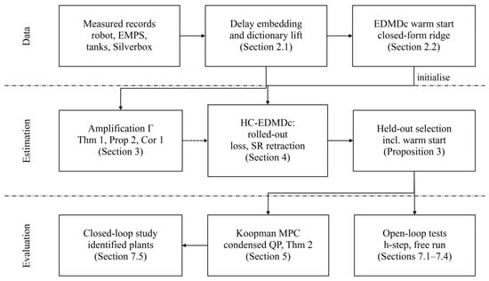
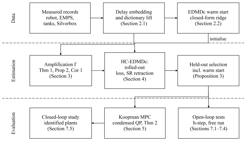
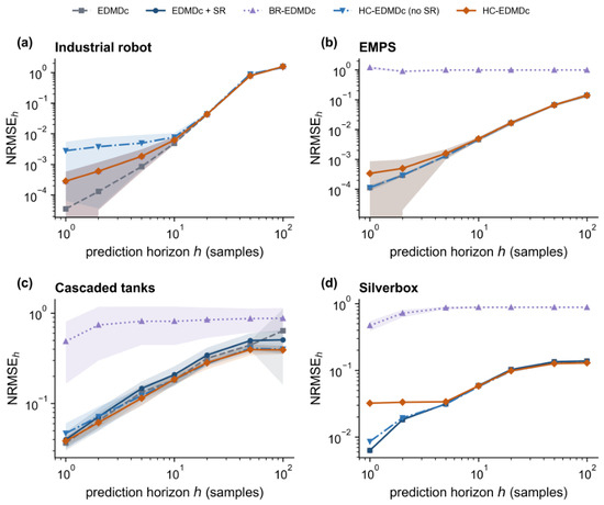
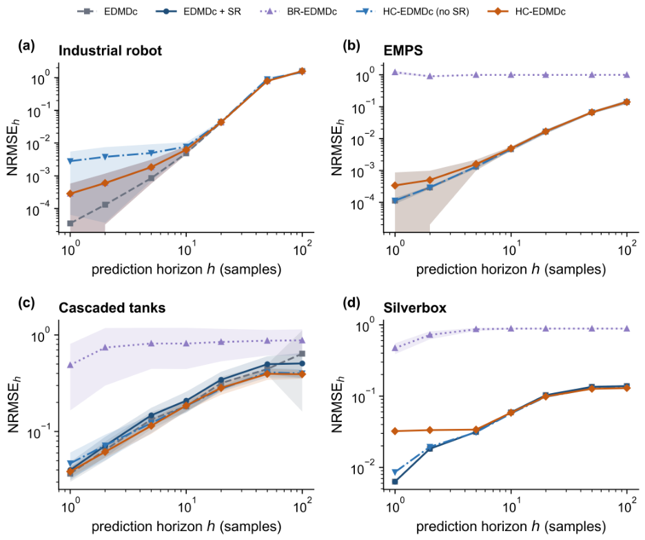
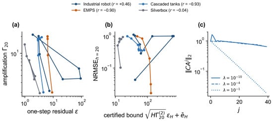
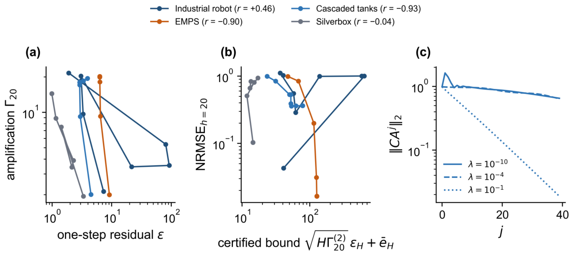
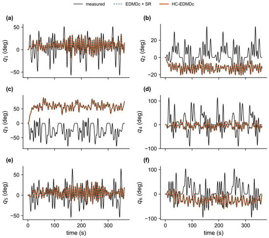
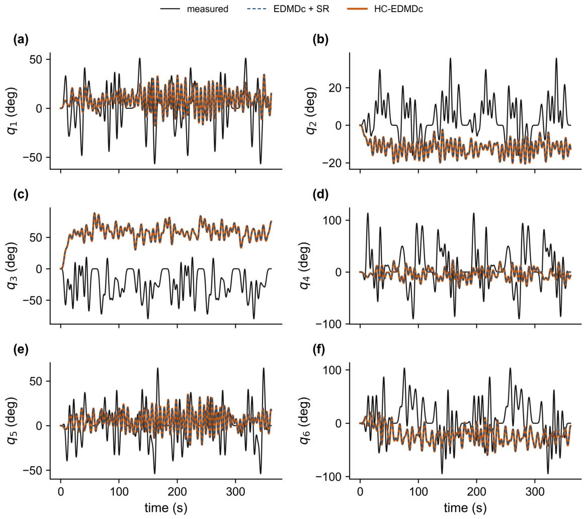
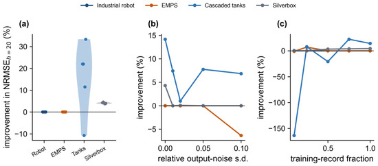
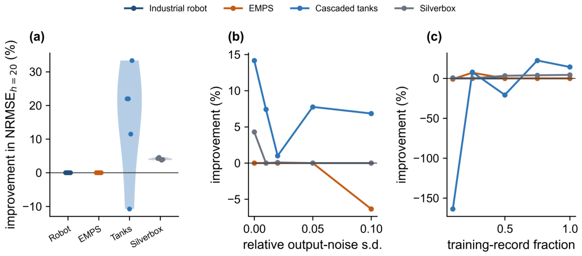
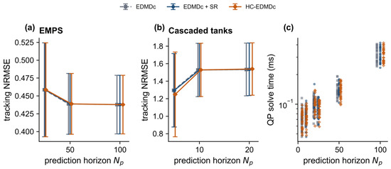
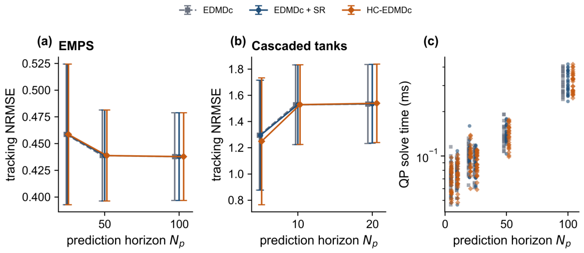

Disclaimer/Publisher’s Note: The statements, opinions and data contained in all publications are solely those of the individual author(s) and contributor(s) and not of MDPI and/or the editor(s). MDPI and/or the editor(s) disclaim responsibility for any injury to people or property resulting from any ideas, methods, instructions or products referred to in the content. |
© 2026 by the authors. Licensee MDPI, Basel, Switzerland. This article is an open access article distributed under the terms and conditions of the Creative Commons Attribution (CC BY) license.