Neural Finite Volume and Mixture-of-Experts Physics-Informed Networks for the Isentropic Cargo–LeRoux Model: An Exact-Solution-Grounded Comparative Study

Abstract

We compare three neural approaches to the Riemann problem of the isentropic Cargo–LeRoux model with an exact solver and with classical Godunov-type schemes. The model has a linearly degenerate contact field and a strictly convex closure that is singular at $a\rho =1$. We pose the star-state system as constrained residual minimisation. Without entropy constraints, the minimiser contains an expansion shock on 78.6% of well-conditioned cases; with entropy bounds on each wave, it is correct on all 1237 solvable cases and identifies all 163 vacuum cases. Eliminating the contact relation reduces the problem to a monotone scalar equation whose root exists, uniquely, exactly when no vacuum forms; a bracketed solve gives the same reliability at about 1/116 of the cost. Godunov schemes built on the two solvers agree to 8 × 10⁻¹⁰, need no fallback, and are 1.4–2.8 times more accurate than Rusanov; without entropy constraints, the scheme forms an expansion shock at the sonic point. At a contact, cell averaging breaks the equilibrium of $p+q$; a contact-consistent update restores it to machine precision on an isolated contact. Over five wave patterns and three seeds, a Mixture-of-Experts physics-informed network matches a first-order Rusanov scheme. A neural finite volume (NFV) scheme fitted to each target is 6–34 times more accurate than Rusanov, but its flux is inconsistent, its error grows 6–19-fold on held-out data, and it produces negative densities near vacuum in one of three seeds. A hybrid scheme’s detector flags every vacuum case, yet its surrogate star states violate the Riemann relations by 18–25%.

1. Introduction

The exact solution of the Riemann problem underlies Godunov-type schemes for compressible flow [1,2,3,4]. A local Riemann problem at every cell interface determines the numerical flux. The accuracy and robustness of the scheme therefore depend directly on the quality of that solution. This dependence makes the Riemann problem a natural target for machine learning [5,6]. Several recent studies train neural networks to reproduce or accelerate the exact or approximate solution, rather than replace the finite-volume framework [7,8,9].

The Cargo–LeRoux model [10] poses a Riemann problem with two features rarely combined in this literature. It is a hyperbolic system of three conservation laws for isentropic flow with an advected potential q that enters the momentum flux. Its van der Waals-type closure is strictly convex in density, but it is singular at $a\rho =1$, where pressure and sound speed diverge. The middle characteristic field is linearly degenerate. The exact Riemann solution consists of a genuinely nonlinear wave, a contact discontinuity and a second genuinely nonlinear wave. Jana and Kuila [11] derived the exact solution. Karna and Satapathy [12] analysed its Lie symmetries, and Sahoo et al. [13] studied wave interactions in the pressureless variant. Khan et al. [14] implemented a Godunov method for it. None of these studies applies machine learning to the model.

This gap matters for two reasons. First, a linearly degenerate middle field is a known difficulty for multidimensional and learned solvers in related models [15]. Second, two recent neural paradigms, Mixture-of-Experts physics-informed networks [16,17] and neural finite volume methods [15], have not been applied, to our knowledge, to a system that combines a degenerate field with a singular closure. Applying both to the same model, against the same exact solver, isolates how each one handles shocks, contacts and near-vacuum states.

The two wave families behave differently, and the two paradigms respond differently to them. A genuinely nonlinear field compresses into shocks and expands into rarefactions. A linearly degenerate field only advects a jump. A network trained on a smooth residual represents an expanding profile with little effort, but it must fit unbounded gradients to represent a shock [18]. The usual vanishing-viscosity remedy restores an entropy selection principle, and it smooths the discontinuity in exchange. Section 5 quantifies the consequence: the MoE-PINN density error is 4.3–8.3 times larger on the shock-containing patterns than on the purely rarefactive one. A first-order Rusanov scheme shows a ratio of 3.2–5.7 on the same data, so the ratio reflects the cost of discontinuities for any smoothing method, not a feature unique to the network.

The neural finite volume scheme conserves mass, momentum and $\rho q$ exactly through its update. Conservation alone, however, does not deliver the Lax–Wendroff guarantee; the numerical flux must also be consistent with the physical flux [19]. We measure this consistency directly and find relative mismatches of 0.02–8.7 on the visited states. The trained flux therefore reproduces its training target closely but does not inherit a convergence guarantee, and its accuracy falls by a factor of 6–19 on a held-out configuration.

The hybrid scheme tests a third principle: a classical solver’s own failure can be predicted more cheaply than it can be repaired. The exact solver fails only on a characterisable subset of data, near vacuum or near the equation-of-state singularity. A detector built from that characterisation is reused, with its logical form unchanged, from an HLLC-based hybrid scheme [20]. The detector isolates this subset reliably; the learned fallback does not yet supply accurate star states inside it.

A fourth finding concerns classical schemes. Across a contact, u and $p+q$ are continuous, while $\rho$, p and q jump. Cell averaging of $\rho$ and $\rho q$ breaks the balance of $p+q$ in smeared cells. A conservative scheme then generates a spurious velocity and a density dip at the contact. This mechanism resembles the pressure oscillations of multicomponent flow computations [21]. It persists under grid refinement, and it appears with the exact Godunov flux as well as with the Rusanov flux.

The comparison also raises two classical questions. Which optimisation strategy should solve the star-state system, and how does that choice affect a Godunov scheme built on it? The system is two nonlinear equations, and Newton-type solvers fail near vacuum and near the singularity. Residual minimisation over an admissible set is a natural alternative because it can impose positivity and entropy admissibility as constraints. We show that it returns the physical star state only when the entropy constraints are explicit. The contact relation then reduces it to one monotone equation, which settles existence, uniqueness and vacuum detection at once and gives a solver that cannot diverge.

This paper makes eight contributions. Section 2 gives an exact Riemann solver with a closed-form Riemann invariant, a convexity and fan-ordering analysis and a validation. Section 3 describes the MoE-PINN and its vanishing-viscosity regularisation. Section 4 describes the NFV scheme, its consistency and its time-step control. Section 5 compares both methods with the exact solution and a Rusanov baseline on five configurations, and it reports PDE residuals, admissibility and oscillation measures for every method. Section 6 evaluates a hybrid exact–neural scheme with a multi-seed design and cross-validates the exact solver against published test cases. Section 7 poses the star-state system as constrained residual minimisation, shows that the entropy constraints decide its outcome, reduces it to a monotone scalar equation with existence and uniqueness, and compares ten solution strategies. Section 8 builds Godunov schemes on these solvers, including residual-minimisation solvers with and without entropy constraints, and compares them with HLL and Rusanov for accuracy, robustness, entropy consistency and contact consistency. Section 9 extends the model to two dimensions and discusses irregular geometries.

2. Governing Equations and the Exact Riemann Solver

2.1. Governing System

Following [11,14], the isentropic Cargo–LeRoux system in conservative form is

$${\displaystyle \frac{\partial U}{\partial t}}+{\displaystyle \frac{\partial F\left(U\right)}{\partial x}}=0,U=\left(\begin{array}{c}\rho \\ \rho q\\ \rho u\end{array}\right),F\left(U\right)=\left(\begin{array}{c}\rho u\\ \rho qu\\ \rho u^2+p+q\end{array}\right),$$

(1)

where $\rho >0$ is density, u is velocity and q is the potential. The pressure follows the van der Waals-type closure

$$p\left(\rho \right)=A{\left({\displaystyle \frac{\rho }{1-a\rho }}\right)}^{\gamma },0<a\rho <1,\gamma >1.$$

(2)

which implies,

$$p^{\prime }\left(\rho \right)={\displaystyle \frac{A\gamma {\rho }^{\gamma -1}}{{(1-a\rho )}^{\gamma +1}}}>0,p^{″}\left(\rho \right)={\displaystyle \frac{A\gamma {\rho }^{\gamma -2}}{{(1-a\rho )}^{\gamma +2}}}\left(\gamma -1+2a\rho \right)>0.$$

(3)

The closure is therefore strictly increasing and strictly convex on the physical domain. It departs from the polytropic law through its singularity at $a\rho \to 1$, where p and $p^{\prime }$ diverge, and not through any loss of convexity. All experiments use $A=0.5$, $a=0.035$ and $\gamma =1.4$. Reference [14] uses the same constants, and Section 6.2 compares the exact solver with its published test cases.

In primitive variables $V={(\rho ,q,u)}^T$, system (1) takes the quasi-linear form $V_t+A\left(V\right)V_x=0$ with

$$A\left(V\right)=\left(\begin{array}{ccc}u& 0& \rho \\ 0& u& 0\\ p^{\prime }\left(\rho \right)/\rho & 1/\rho & u\end{array}\right),$$

(4)

whose characteristic polynomial factors as $(u-\lambda )[{(u-\lambda )}^2-{\sigma }^2]=0$ with

$$\sigma \left(\rho \right)=\sqrt{p^{\prime }\left(\rho \right)}=\sqrt{{\displaystyle \frac{A\gamma {\rho }^{\gamma -1}}{{(1-a\rho )}^{\gamma +1}}}}.$$

(5)

The eigenvalues ${\lambda }_1=u-\sigma$, ${\lambda }_2=u$ and ${\lambda }_3=u+\sigma$ are real and distinct whenever $\rho >0$ and $a\rho <1$, so the system is strictly hyperbolic on the physical domain. For fields 1 and 3, $\nabla \lambda ·r$ is proportional to $\rho p^{″}+2p^{\prime }$, which is positive by (3); both fields are genuinely nonlinear. Field 2 is linearly degenerate and carries the contact discontinuity, across which u and $p+q$ are continuous, while $\rho$ and q may jump.

2.2. Riemann Invariants in Closed Form

Let $\mathrm{\Phi }\left(\rho \right)={\int }_0^{\rho }\sigma \left(\xi \right)/\xi d\xi$. The integrand equals $\sqrt{A\gamma }{\rho }^{(\gamma -3)/2}{(1-a\rho )}^{-(\gamma +1)/2}$, and it is the derivative of a power of $\rho /(1-a\rho )$. Hence

$$\mathrm{\Phi }\left(\rho \right)={\displaystyle \frac{2\sqrt{A\gamma }}{\gamma -1}}{\left({\displaystyle \frac{\rho }{1-a\rho }}\right)}^{(\gamma -1)/2}={\displaystyle \frac{2\sigma \left(\rho \right)(1-a\rho )}{\gamma -1}},$$

(6)

which reduces to the polytropic invariant $2\sigma /(\gamma -1)$ when $a=0$. The closed form is exact and costs one power evaluation. An earlier version of our solver tabulated $\mathrm{\Phi }$ by quadrature and interpolated it with a cubic spline on a uniform grid of spacing 0.007. That table was accurate to ${10}^{-7}$ for $\rho \ge 0.1$, but its error reached 0.04 at $\rho =0.01$ and 0.49 at $\rho ={10}^{-3}$. Near vacuum this error moved the star density of Configuration 2 (Section 6) from its correct value 0.00282 to 0.00462. All results in this paper use (6).

Across a 1-rarefaction from $({\rho }_l,u_l)$ to the star state $({\rho }_{-},u_{-})$, constancy of $u+\mathrm{\Phi }\left(\rho \right)$ gives

$$u_{-}=u_l-[\mathrm{\Phi }\left({\rho }_{-}\right)-\mathrm{\Phi }\left({\rho }_l\right)],{\rho }_{-}\le {\rho }_l.$$

(7)

Across a 3-rarefaction from the star state $({\rho }_{+},u_{+})$ to $({\rho }_r,u_r)$, constancy of $u-\mathrm{\Phi }\left(\rho \right)$ gives

$$u_{+}=u_r-[\mathrm{\Phi }\left({\rho }_r\right)-\mathrm{\Phi }\left({\rho }_{+}\right)],{\rho }_{+}\le {\rho }_r.$$

(8)

Remark 1

(sign check of the 3-rarefaction relation). Relation (8) agrees with the third-family invariant of Table 1 and with Table 1 and Equation (16) of [14]. Transcribing (7) to field 3 without using that field’s own invariant gives the sign-flipped candidate $u_{+}=u_r+[\mathrm{\Phi }\left({\rho }_r\right)-\mathrm{\Phi }\left({\rho }_{+}\right)]$. A rarefaction fan requires $u_{+}+\sigma \left({\rho }_{+}\right)\le u_r+\sigma \left({\rho }_r\right)$. On 7200 pairs $0<{\rho }_{+}<{\rho }_r\le 25$, relation (8) satisfies this ordering in every case, while the sign-flipped candidate violates it in 4384 cases (60.9%). Our implementation uses (8); we use the check only as a safeguard against this transcription error, and we attribute no error to the published literature.

Table 1. Riemann invariants of the three characteristic fields; $\mathrm{\Phi }$ is given in closed form by (6).

Field	Invariant 1	Invariant 2
1 (left, $u-\sigma$)	q	$u+\mathrm{\Phi }\left(\rho \right)$
2 (contact, u)	u	$q+p$
3 (right, $u+\sigma$)	q	$u-\mathrm{\Phi }\left(\rho \right)$

2.3. Shocks and the Coupled Nonlinear System

Across a k-shock, the Rankine–Hugoniot conditions give

$${(u_K-u_{*})}^2=[p\left({\rho }_{*}\right)-p\left({\rho }_K\right)]\left({\displaystyle \frac{1}{{\rho }_K}}-{\displaystyle \frac{1}{{\rho }_{*}}}\right),$$

(9)

so a 1-shock (${\rho }_{-}>{\rho }_l$) and a 3-shock (${\rho }_{+}>{\rho }_r$) satisfy

$$u_{-}=u_l-\sqrt{[p\left({\rho }_{-}\right)-p\left({\rho }_l\right)]\left({\displaystyle \frac{1}{{\rho }_l}}-{\displaystyle \frac{1}{{\rho }_{-}}}\right)},u_{+}=u_r+\sqrt{[p\left({\rho }_{+}\right)-p\left({\rho }_r\right)]\left({\displaystyle \frac{1}{{\rho }_r}}-{\displaystyle \frac{1}{{\rho }_{+}}}\right)}.$$

(10)

Mass conservation gives the shock speed $S=({\rho }_{*}{u}_{*}-{\rho }_K{u}_K)/({\rho }_{*}-{\rho }_K)$. Let ${\omega }_1,{\omega }_3$ denote the branch functions that return the shock relation (10) or the rarefaction relation (7)/(8). The Riemann problem reduces to two nonlinear equations for ${\rho }_{-},{\rho }_{+}$:

$$u_l-{\omega }_1({\rho }_{-},{\rho }_l)=u_r+{\omega }_3({\rho }_{+},{\rho }_r),q_l+p\left({\rho }_{-}\right)=q_r+p\left({\rho }_{+}\right).$$

(11)

We solve (11) with MINPACK’s hybrid Powell method (SciPy fsolve), a Newton-type method with a trust-region safeguard, started from $({\rho }_l,{\rho }_r)$. Reference solutions in Section 5 and Section 6 use several starting points and keep the converged root with the smallest residual.

Vacuum generation. Both nonlinear waves are rarefactions when the data separate. If

$$u_r-u_l\ge \mathrm{\Phi }\left({\rho }_l\right)+\mathrm{\Phi }\left({\rho }_r\right),$$

(12)

the two fans detach and a vacuum forms, because (7) and (8) cannot reach a common velocity with ${\rho }_{\pm }>0$ and $\mathrm{\Phi }\left(0\right)=0$. System (11) then has no root. The solver of this section does not construct the vacuum solution, and such data fall into the flagged set of Section 6. Section 7 generalises (12) to $\Delta q\ne 0$ and gives a solver that returns the star state or proves the vacuum.

2.4. Validation

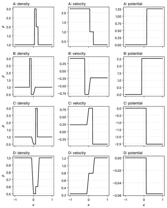
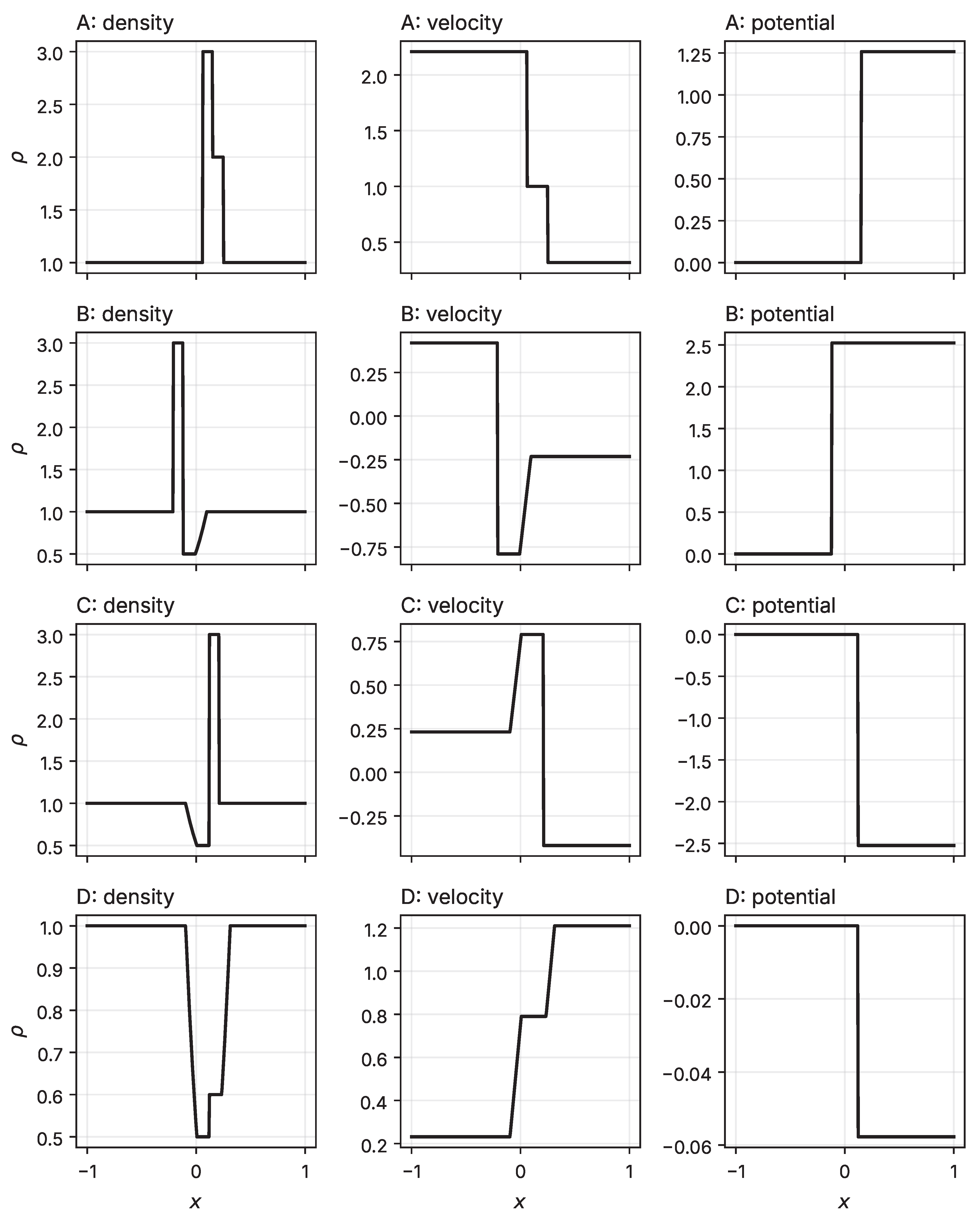
We validate the implementation by construction. For each configuration, we choose a target $({\rho }_{-},{\rho }_{+},u^{*})$, back-solve the far-field states, and check that the forward solve recovers the target. Table 2 lists the back-solved states, so that every configuration can be reproduced. The forward solve recovers every target with a residual below 10⁻¹¹. Configurations A–D fix ${\rho }_l={\rho }_r=1$ as a construction choice, and Configuration E uses unequal far-field densities (${\rho }_l=2$, ${\rho }_r=0.5$). Figure 1 shows the exact solutions.

Table 2. Self-consistency validation ($A=0.5$, $a=0.035$, $\gamma =1.4$, $q_l=0$). Far-field states are back-solved from the target star state; t./r. = target/recovered; res. = Euclidean residual of (11) at the recovered root.

Config.	${\mathit{\rho }}_{\mathit{l}}$	${\mathit{u}}_{\mathit{l}}$	${\mathit{\rho }}_{\mathit{r}}$	${\mathit{u}}_{\mathit{r}}$	${\mathit{q}}_{\mathit{r}}$	${\mathit{\rho }}_{-}$ (t./r.)	${\mathit{\rho }}_{+}$ (t./r.)	${\mathit{u}}^{*}$ (t./r.)	res.
A	1.0	2.2092	1.0	0.3162	1.2582	3.0000/3.0000	2.0000/2.0000	$1.0000$/$1.0000$	$1.0\times {10}^{-13}$
B	1.0	0.4193	1.0	−0.2313	2.5247	3.0000/3.0000	0.5000/0.5000	$-0.7899$/$-0.7899$	$4.4\times {10}^{-16}$
C	1.0	0.2313	1.0	−0.4193	−2.5247	0.5000/0.5000	3.0000/3.0000	$0.7899$/$0.7899$	0
D	1.0	0.2313	1.0	1.2100	−0.0577	0.5000/0.5000	0.6000/0.6000	$0.7899$/$0.7899$	$3.1\times {10}^{-15}$
E	2.0	1.8427	0.5	0.4244	3.7753	4.0000/4.0000	1.0000/1.0000	$1.0000$/$1.0000$	$2.3\times {10}^{-12}$

A: shock–contact–shock; B: shock–contact–rarefaction; C: rarefaction–contact–shock; D: rarefaction–contact–rarefaction; E: shock–contact–shock with ${\rho }_l\ne {\rho }_r$.

Figure 1. Exact solutions of Configurations A–D (Table 2) at $t=0.15$.

3. Mixture-of-Experts Physics-Informed Networks

3.1. Why a Pointwise Residual Is the Wrong Object at a Discontinuity

A standard PINN minimises the pointwise residual $\mathcal{R}\left[U_{\theta }\right]={\partial }_t{U}_{\theta }+{\partial }_{x}F\left(U_{\theta }\right)$ at collocation points. This residual is well posed only where the solution is classically differentiable. At a shock, ${\partial }_{x}F\left(U\right)$ is a distribution, so minimising $\mathcal{R}$ pointwise forces the network to smooth the step. The vanishing-viscosity principle addresses this:

$${\mathcal{R}}_{\epsilon }\left[U_{\theta }\right]={\partial }_t{U}_{\theta }+{\partial }_{x}F\left(U_{\theta }\right)-\epsilon {\left({\partial }_{xx}{\rho }_{\theta },0,0\right)}^T,$$

(13)

with $\epsilon$ annealed geometrically from 0.05 to ${\epsilon }_T=1.0\times {10}^{-3}$ over training. Kružkov theory [22,23] shows that the vanishing-viscosity limit selects the admissible weak solution. Two consequences follow. A non-zero $\epsilon$ smooths the shock over a width that scales with $\epsilon$, independently of network capacity. A rarefaction has small ${\partial }_{xx}\rho$, so the regularisation costs the network little on smooth waves. Because the viscous term acts on the mass equation only, the regularised and actual residuals differ only in that component (Section 5.2).

3.2. Mixture-of-Experts Architecture

We fit a gated mixture

$$U_{\theta }(x,t)={\displaystyle \sum _{i=1}^m}{\lambda }_i(x,t)f_i(x,t;{\theta }_i),{\lambda }_i={\displaystyle \frac{\exp g_i(x,t;{\theta }_g)}{{\sum }_j\exp g_j(x,t;{\theta }_g)}}.$$

(14)

We use $m=2$ experts. Each expert applies $\sin (·)$ to its input coordinates and then three hidden layers of 20 tanh units. The gate is a tanh network with two hidden layers of 16 units. The density output passes through a softplus and a floor of ${10}^{-3}$, which enforces $\rho >0$ by construction. The loss is the mean-square residual (13) at 1500 collocation points, resampled uniformly in $[x_{\min },x_{\max }]\times [0,T]$ at every iteration, plus 20 times the mean-square initial-condition error at 300 points. We train with Adam (learning rate $2\times {10}^{-3}$) for 2000 iterations. The loss contains no boundary term and no gate-sparsity term. Each new Riemann problem requires a new training run.

4. Neural Finite Volume

4.1. Conservation, Consistency and the Lax–Wendroff Argument

NFV does not represent $U(x,t)$ directly. It trains a network ${\mathrm{\Phi }}_{\theta }$ to act as the numerical flux in the conservative update

$$U_i^{n+1}=U_i^n-{\displaystyle \frac{\Delta t}{\Delta x}}\left[{\mathrm{\Phi }}_{\theta }(U_i^n,U_{i+1}^n)-{\mathrm{\Phi }}_{\theta }(U_{i-1}^n,U_i^n)\right].$$

(15)

Update (15) conserves $\rho$, $\rho q$ and $\rho u$ exactly, whatever ${\mathrm{\Phi }}_{\theta }$ is. The Lax–Wendroff theorem [19] adds a second requirement: a convergent conservative scheme converges to a weak solution only if its flux is consistent, ${\mathrm{\Phi }}_{\theta }(U,U)=F\left(U\right)$. An unconstrained network does not satisfy this identity. We measure the relative inconsistency

$${\kappa }_k={\displaystyle \frac{\parallel {\mathrm{\Phi }}_{\theta ,k}(U,U)-F_k{\left(U\right)\parallel }_2}{\parallel F_k{\left(U\right)\parallel }_2}}$$

(16)

over all states visited in a rollout. It ranges from 0.02 to 8.7 (median 0.98) over the 24 trained networks of Section 5 and Section 6. The Lax–Wendroff guarantee therefore does not apply to the trained NFV. Its sharp shocks come from supervised fitting, not from a convergence theorem.

The flux network takes the two adjacent conserved states (6 inputs) and has two hidden layers of 30 tanh units. The grid has 80 cells, zero-gradient boundaries and CFL number 0.4. For each configuration, we unroll (15) from the Riemann data to $t=T$, compare the final conserved state with the exact cell averages (five-point quadrature per cell), and backpropagate through the unrolled graph. We train with Adam (learning rate $3\times {10}^{-3}$, gradient norm clipped at 1) for 500 epochs. The reported NFV error on a configuration is thus a fitting error on that configuration’s own target; Section 5.1 measures transfer to unseen data.

4.2. Time-Step Control

Explicit schemes of form (15) with an upwind-type flux are stable under $\Delta t\le \mathrm{CFL}·\Delta x/{\max }_i\left(\right|u_i|+\sigma \left({\rho }_i\right))$. During autoregressive rollout, the network sees its own predictions, and the wave speeds of those predictions can exceed the speeds of the initial data. We therefore recompute $\Delta t$ from the current predicted state at every step and detach this computation from the gradient graph. To test whether a fixed step is harmful, we repeat the training of Configurations A–E with $\Delta t$ fixed from the initial data. At nominal CFL 0.4, the realised CFL number rises to at most 0.63, and training remains stable. At nominal CFL 0.8, the realised CFL number reaches 0.95–5.24 in Configurations A–C, yet 0 of 9 runs diverge, and the final density error stays within 13% of the adaptive runs. A learned flux is not bound by the stability analysis of an upwind flux, and the fit compensates for the larger step. We keep the adaptive step as a safeguard because nothing guarantees this compensation, but our experiments do not show that a fixed step causes divergence.

5. Comparison of MoE-PINN and NFV with the Exact Solution

We evaluate both methods on Configurations A–D at $t=0.15$ on $[-1,1]$, with three random seeds (0, 1, 2) per method. We add a first-order Rusanov (local Lax–Friedrichs) scheme [24] on the same 80-cell grid as a classical reference. MoE-PINN errors use 200 equispaced points; NFV and Rusanov errors use exact cell averages.

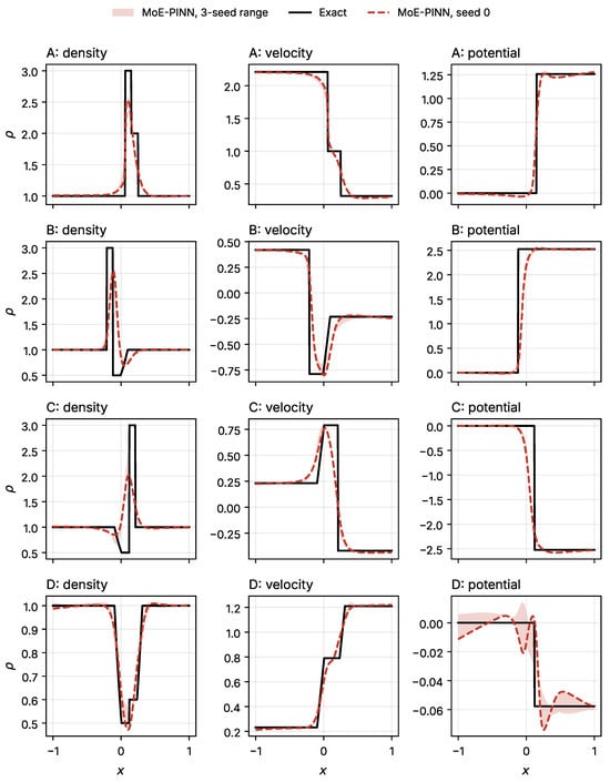
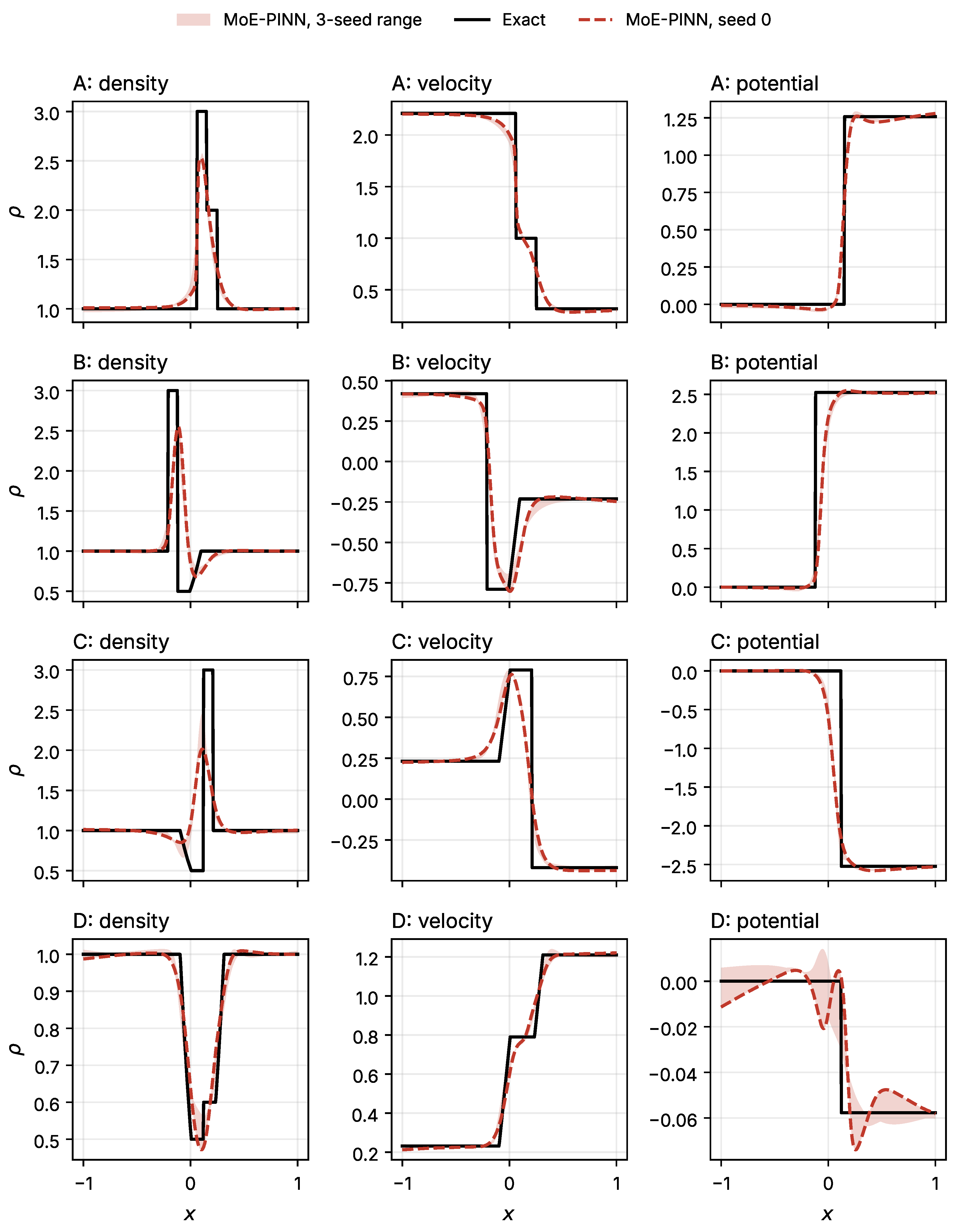
The MoE-PINN density error on the shock-containing patterns A–C is 4.3–8.3 times its error on the purely rarefactive pattern D. The velocity error grows by a factor of 2.7–3.0, the potential error by 5.7–17.3, and the summed error by 3.8–7.1. The mean shock peaks fall short of the exact value 3.0 by 15–25% (Table 3, Figure 2), which is the smoothing that (13) predicts. A first-order Rusanov scheme shows a density-error ratio of 3.2–5.7 on the same data, and the MoE-PINN density error is 0.94–1.36 times that of Rusanov. MoE-PINN thus performs like a first-order classical scheme on an 80-cell grid.

Table 3. MoE-PINN $L_1$ errors against the exact solution, mean ± standard deviation over 3 seeds.

Config.	${\mathit{L}}_1\left(\mathit{\rho }\right)$	${\mathit{L}}_1\left(\mathit{u}\right)$	${\mathit{L}}_1\left(\mathit{q}\right)$	Peak $\mathit{\rho }$ (Exact: 3, 3, 3, 1)
A	$0.086\pm 0.009$	$0.061\pm 0.005$	$0.037\pm 0.002$	$2.54\pm 0.03$
B	$0.147\pm 0.006$	$0.060\pm 0.003$	$0.101\pm 0.008$	$2.42\pm 0.10$
C	$0.164\pm 0.004$	$0.066\pm 0.001$	$0.114\pm 0.006$	$2.24\pm 0.18$
D	$0.020\pm 0.000$	$0.022\pm 0.002$	$0.007\pm 0.000$	$1.01\pm 0.00$

Figure 2. MoE-PINN against the exact solution, Configurations A–D, $t=0.15$. Dashed: seed 0; shading: range over seeds 0–2.

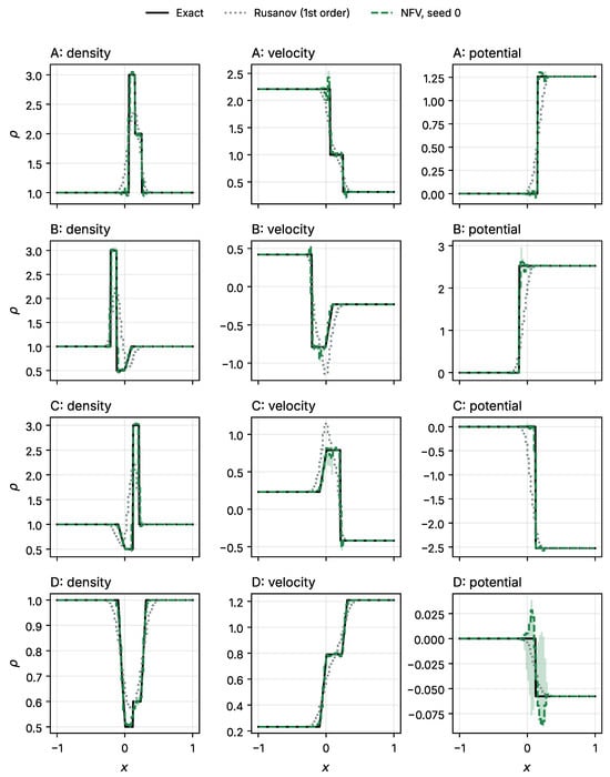
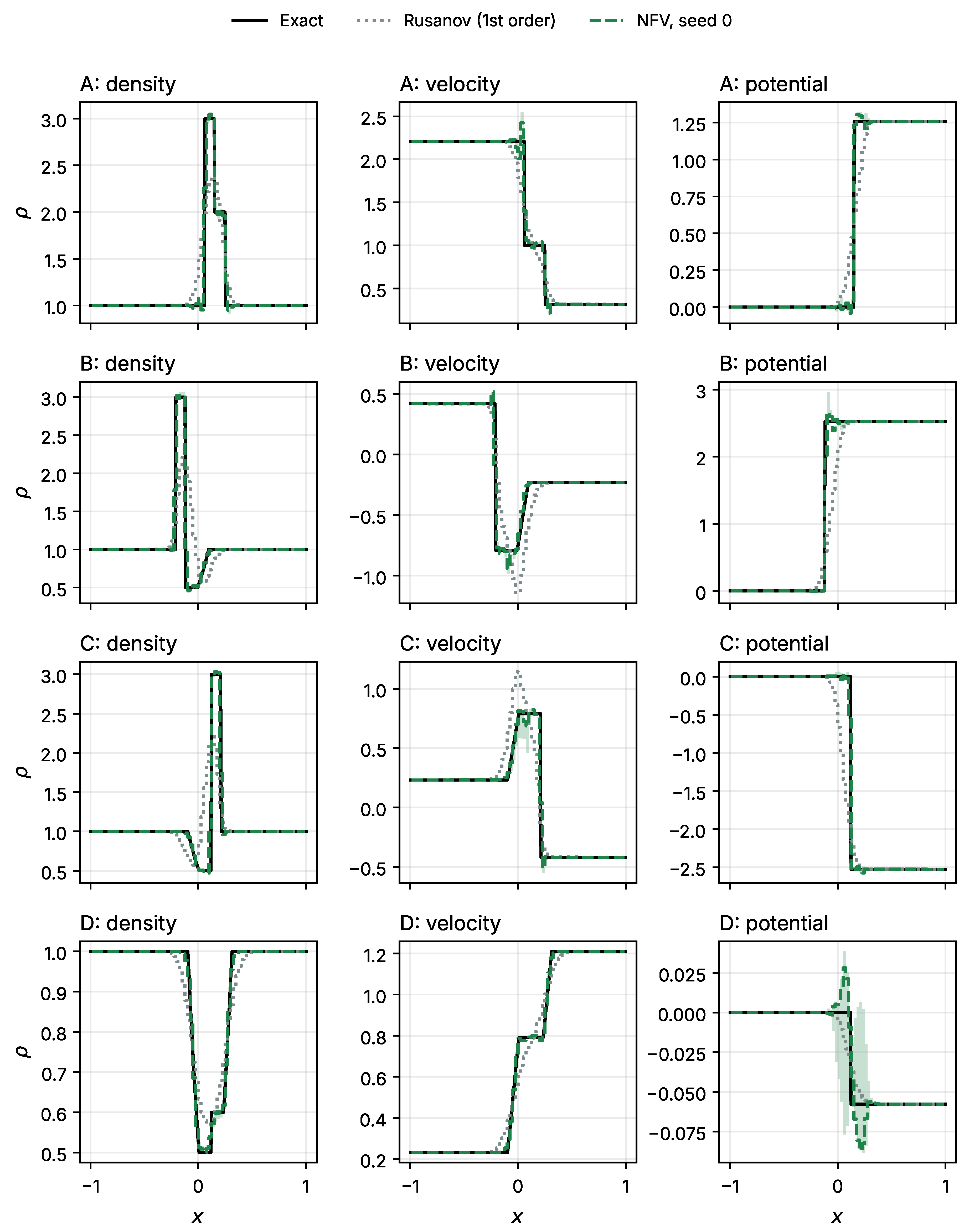
The NFV density error is 6–34 times smaller than that of Rusanov on the same grid, and it recovers the shock peaks to within 2% (Table 4). This accuracy is a fit to each configuration’s own exact solution (Section 4). Figure 3 shows the profiles; NFV places the shocks correctly but adds cell-scale oscillations near steep features, which Section 5.3 quantifies.

Table 4. NFV $L_1$ errors against exact cell averages, mean ± standard deviation over 3 seeds, and the first-order Rusanov scheme on the same 80-cell grid (deterministic, one run).

	NFV (3 Seeds)				Rusanov
Config.	${\mathit{L}}_{\mathbf{1}}\left(\mathit{\rho }\right)$	${\mathit{L}}_{\mathbf{1}}\left(\mathit{u}\right)$	${\mathit{L}}_{\mathbf{1}}\left(\mathit{q}\right)$	Peak $\mathit{\rho }$	${\mathit{L}}_{\mathbf{1}}\left(\mathit{\rho }\right)$	${\mathit{L}}_{\mathbf{1}}\left(\mathit{u}\right)$	${\mathit{L}}_{\mathbf{1}}\left(\mathit{q}\right)$
A	$0.0080\pm 0.0012$	$0.0122\pm 0.0007$	$0.0054\pm 0.0010$	$3.06\pm 0.01$	0.067	0.037	0.038
B	$0.0044\pm 0.0023$	$0.0091\pm 0.0012$	$0.0110\pm 0.0045$	$3.03\pm 0.03$	0.120	0.057	0.093
C	$0.0035\pm 0.0005$	$0.0118\pm 0.0062$	$0.0039\pm 0.0004$	$3.03\pm 0.00$	0.120	0.057	0.093
D	$0.0033\pm 0.0004$	$0.0032\pm 0.0003$	$0.0045\pm 0.0027$	$1.00\pm 0.00$	0.021	0.023	0.002

Figure 3. NFV against exact cell averages, Configurations A–D, $t=0.15$, 80 cells. Dashed green: NFV, seed 0; light-green shading: range of the NFV solutions over seeds 0–2 (visible where the seeds differ, e.g., the potential of Configuration D); dotted grey: first-order Rusanov on the same grid.

5.1. Transfer to a Held-Out Configuration

To measure generalisation, we trained one flux network jointly on Configurations A–D and evaluated it on Configuration E, which it never saw. Configuration E has the same wave pattern as A but different density levels.

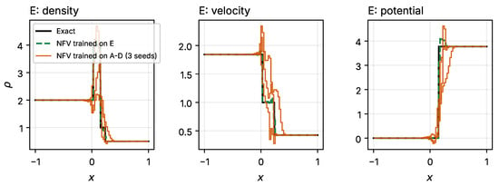
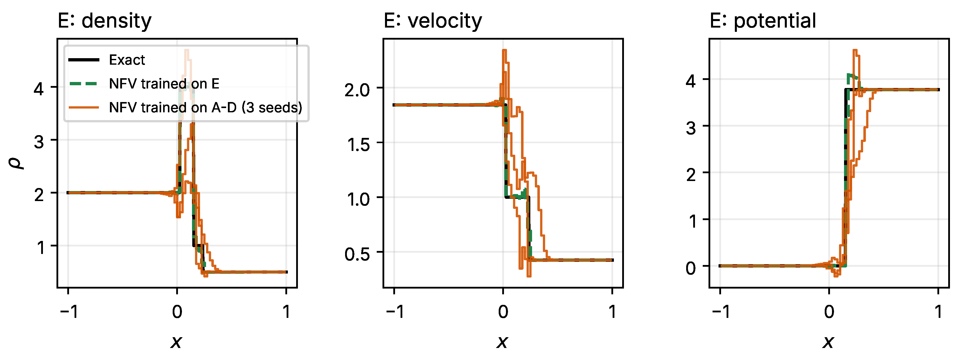
On the held-out configuration, the NFV density error rises to 0.062–0.181, which is 6–19 times its error when trained on E itself (Table 5). On its training configurations A–D, the same jointly trained network reaches 0.008–0.048. The held-out error is comparable to those of MoE-PINN and Rusanov. The peak density ranges from 2.21 to 4.69 across seeds, against an exact value of 4.0, and the velocity overshoots its exact range by up to 35% (Figure 4). The NFV advantage in Table 4 therefore holds on the data it was fitted to, and largely disappears on new data.

Table 5. Configuration E: $L_1$ errors and peak density (exact peak 4.0), mean ± standard deviation over 3 seeds; Rusanov is one deterministic run.

Method	${\mathit{L}}_1\left(\mathit{\rho }\right)$	${\mathit{L}}_1\left(\mathit{u}\right)$	${\mathit{L}}_1\left(\mathit{q}\right)$	Peak $\mathit{\rho }$
NFV trained on E	$0.010\pm 0.003$	$0.006\pm 0.003$	$0.027\pm 0.010$	$4.06\pm 0.00$
NFV trained on A–D (E held out)	$0.124\pm 0.049$	$0.069\pm 0.040$	$0.123\pm 0.048$	$3.40\pm 1.02$
MoE-PINN	$0.114\pm 0.002$	$0.070\pm 0.007$	$0.067\pm 0.003$	$3.79\pm 0.03$
Rusanov (first order)	0.130	0.071	0.127	3.29

Figure 4. Configuration E, excluded from training of the jointly trained network. Dashed: NFV trained on E (seed 0); solid orange: NFV trained on A–D (seeds 0–2).

5.2. Substituting the Predictions into the Governing Equations

Error against the exact solution does not show whether a prediction satisfies the PDE. We therefore substitute every output into the conservation law in two forms. For MoE-PINN, which is differentiable, we evaluate the strong residual (13) at 20,000 fresh points drawn uniformly in $[x_{\min },x_{\max }]\times [0.02T,T]$, none of which is a training point. We report it separately for points within 0.05 of an exact discontinuity path and for the remaining smooth region, both with $\epsilon ={\epsilon }_T$ (regularised) and with $\epsilon =0$ (actual PDE).

For all methods, including the exact solution, we evaluate the weak (integral) residual on space–time control volumes $[x_a,x_b]\times [t_a,t_b]$,

$$r={\int }_{x_a}^{x_b}\left[U(x,t_b)-U(x,t_a)\right]dx+{\int }_{t_a}^{t_b}\left[F\left(U(x_b,t)\right)-F\left(U(x_a,t)\right)\right]dt,$$

(17)

which vanishes for every weak solution, shocks included. We use 9 columns with edges at the centres of every eighth NFV cell and 5 time slabs, and we normalise $|r_k|$ by $(x_b-x_a)$ times the range of conserved component k in the exact solution. For NFV and Rusanov, the solution is piecewise constant in x and t, and F is the physical flux at the cell centres. For MoE-PINN and the exact solution, we use midpoint quadrature with 400 points in x and 200 in t; the exact solution’s residual measures the quadrature error.

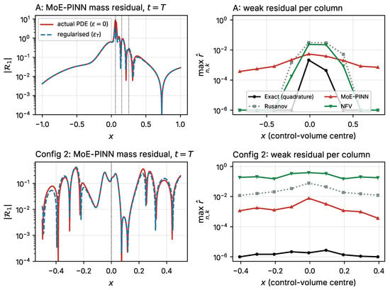
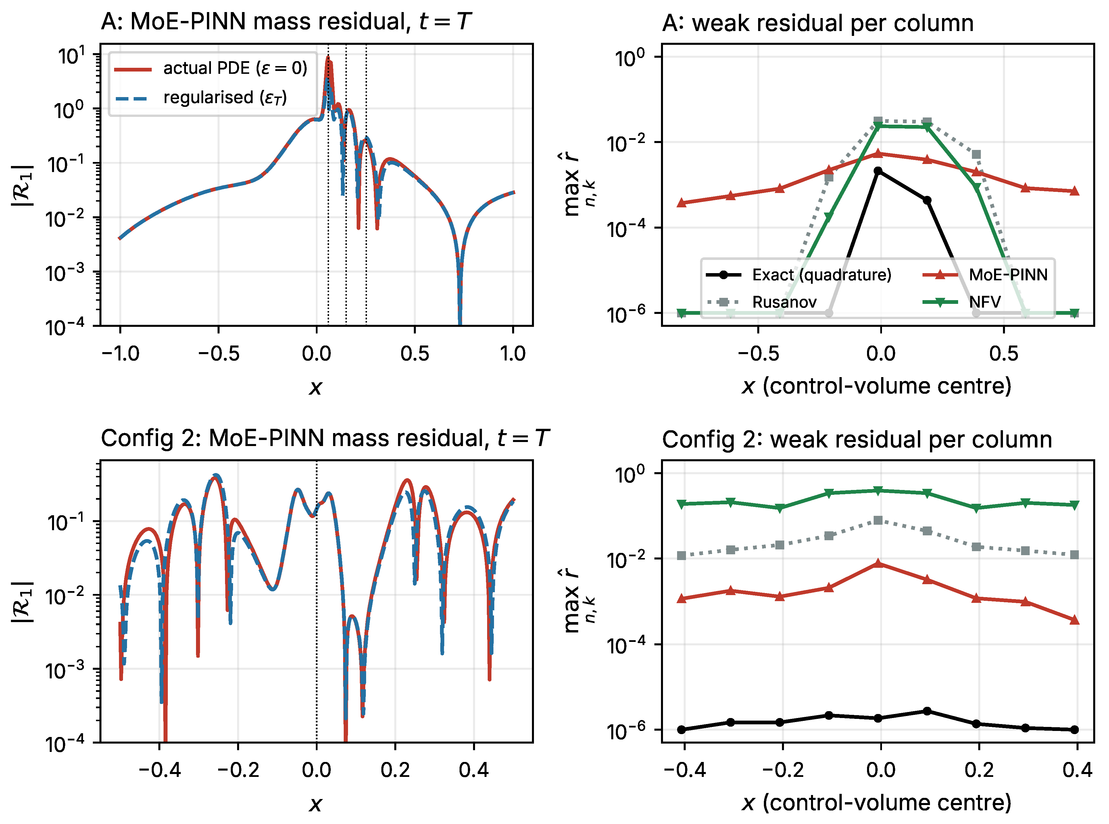
Three results follow from Table 6 and Figure 5. First, MoE-PINN does not satisfy the PDE pointwise. Its mass residual is 0.10–0.22 in smooth regions of the shock-containing configurations and 0.52–1.20 near discontinuities, 4–10 times larger. Second, the regularisation changes only the mass equation near shocks, where it lowers the RMS residual by 4–54%; the regularised residual therefore understates the PDE violation. Third, in the integral sense all methods conserve to within a few per cent of the state range: the maximum weak residual is 0.004–0.021 for MoE-PINN and 0.024–0.070 for NFV, against 0.025–0.061 for Rusanov and 0.0009–0.0029 for the exact solution. The MoE-PINN error is small but spread over the whole domain, while those of NFV and Rusanov are confined to the columns that contain waves (Figure 5). The discrete residuals of NFV and Rusanov carry an $O(\Delta x)$ consistency error near discontinuities, so their weak residuals and that of MoE-PINN are comparable in magnitude, not in kind. Near vacuum (Configuration 2), the NFV weak residual reaches 0.43, six times larger than on any other configuration.

Table 6. Residual checks, mean over 3 seeds. Strong residual (RMS) of MoE-PINN for the mass equation (smooth region; near discontinuities, actual PDE and regularised) and the largest of the $\rho q$ and momentum equations (smooth; near). Weak residual: maximum normalised $\left|r\right|$ of (17) over control volumes and components.

	MoE-PINN, Mass Eq.			MoE-PINN, Other Eqs.		Weak Residual, Max
Config.	Smooth	Near ($\mathit{\epsilon }=\mathbf{0}$)	Near (${\mathit{\epsilon }}_{\mathit{T}}$)	Smooth	Near	Exact	Rusanov	MoE-PINN	NFV
A	0.119	1.205	0.688	0.099	0.497	0.0021	0.031	0.005	0.024
B	0.122	0.524	0.417	0.108	0.427	0.0029	0.025	0.004	0.031
C	0.119	0.567	0.543	0.114	0.485	0.0029	0.027	0.005	0.050
D	0.034	0.117	0.110	0.038	0.156	0.0009	0.026	0.021	0.055
E	0.220	0.925	0.730	0.143	0.707	0.0009	0.052	0.005	0.040
Config. 1	0.096	0.525	0.342	0.080	0.234	0.0015	0.058	0.013	0.070
Config. 3	0.106	0.781	0.360	0.086	0.308	0.0017	0.061	0.006	0.045
Config. 2	0.079	0.328	0.297	0.094	0.490	0.0000	0.078	0.008	0.427

Figure 5. Spatially resolved residuals. (Left): MoE-PINN mass residual $|{\mathcal{R}}_1|$ at $t=T$ (seed 0), actual and regularised; dotted lines mark exact discontinuities. (Right): maximum normalised weak residual per control-volume column (mean over 3 seeds); values below ${10}^{-6}$ are drawn at ${10}^{-6}$. (Top): Configuration A; (Bottom): Configuration 2 (near vacuum, Section 6).

5.3. Admissibility, Oscillations and Limiting

An overshoot that drives $\rho$ to zero or $a\rho$ to one produces a state outside the domain of (2). We therefore record the minimum density over the whole space–time evaluation (a $400\times 61$ grid for MoE-PINN; every cell and step for NFV and Rusanov), the maximum of $a\rho$, and the excursion of $\rho$ and u beyond the range of the exact solution at $t=T$, as a percentage of that range. Table 7 lists these measures for every configuration.

Table 7. Admissibility and oscillation measures (worst seed of 3 for MoE-PINN and NFV). ${\rho }_{\min }$: minimum over space–time; excursion: largest overshoot or undershoot beyond the exact range at $t=T$, in % of that range.

		${\mathit{\rho }}_{\min }$			$\mathit{\rho }$ Excursion (%)			u Excursion (%)
Config.	Exact ${\mathit{\rho }}_{\min }$	MoE	NFV	Rus.	MoE	NFV	Rus.	MoE	NFV	Rus.
A	1	0.8629	0.569	1	1.7	4.2	0.0	1.7	17.8	0.0
B	0.5	0.6832	0.189	0.573	0.0	2.9	0.0	1.6	15.8	29.2
C	0.5	0.6623	0.194	0.573	0.0	1.3	0.0	1.5	10.9	29.2
D	0.5	0.4715	0.482	0.569	5.7	0.0	0.0	3.1	0.0	0.0
E	0.5	0.4062	0.492	0.27	1.4	1.9	6.6	2.5	4.1	78.4
Config. 1	0.68	0.7718	0.513	0.636	0.0	8.8	2.9	4.9	14.4	21.3
Config. 3	1	0.9351	0.936	1	3.8	2.9	0.0	4.4	2.3	0.0
Config. 2	0.002823	0.001119	−0.00304	0.00144	0.2	0.3	0.1	2.5	931.0	0.0

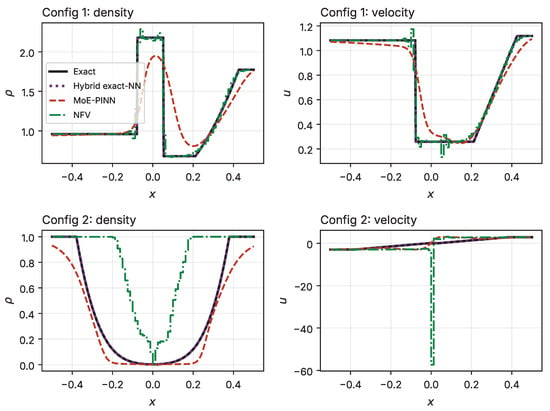
(a) Admissible range. No method produced $a\rho \ge 1$; the largest value of $a\rho$ over all runs was 0.148. MoE-PINN keeps $\rho >0$ by construction, but on Configuration 2 two of three seeds collapsed to the trivial state $\rho \approx {10}^{-3}$ everywhere (peak densities 0.932, 0.001, 0.001; Figure 6), because a vacuum state also makes the residual small. NFV left the admissible range in one seed of Configuration 2: its density fell to −0.0030 in 119 cell steps, and the primitive-variable recovery clamped $\rho$ at ${10}^{-4}$ in 123 cell-steps. This clamp keeps the rollout running but breaks exact conservation. Rusanov kept $\rho >0$ everywhere, and Section 8 shows that a Godunov scheme on the reduced solver of Section 7 stays positive and below $a\rho =1$ even on vacuum-generating and near-singular data.

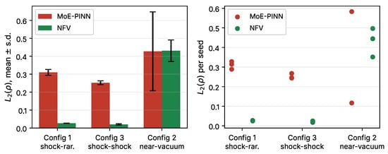
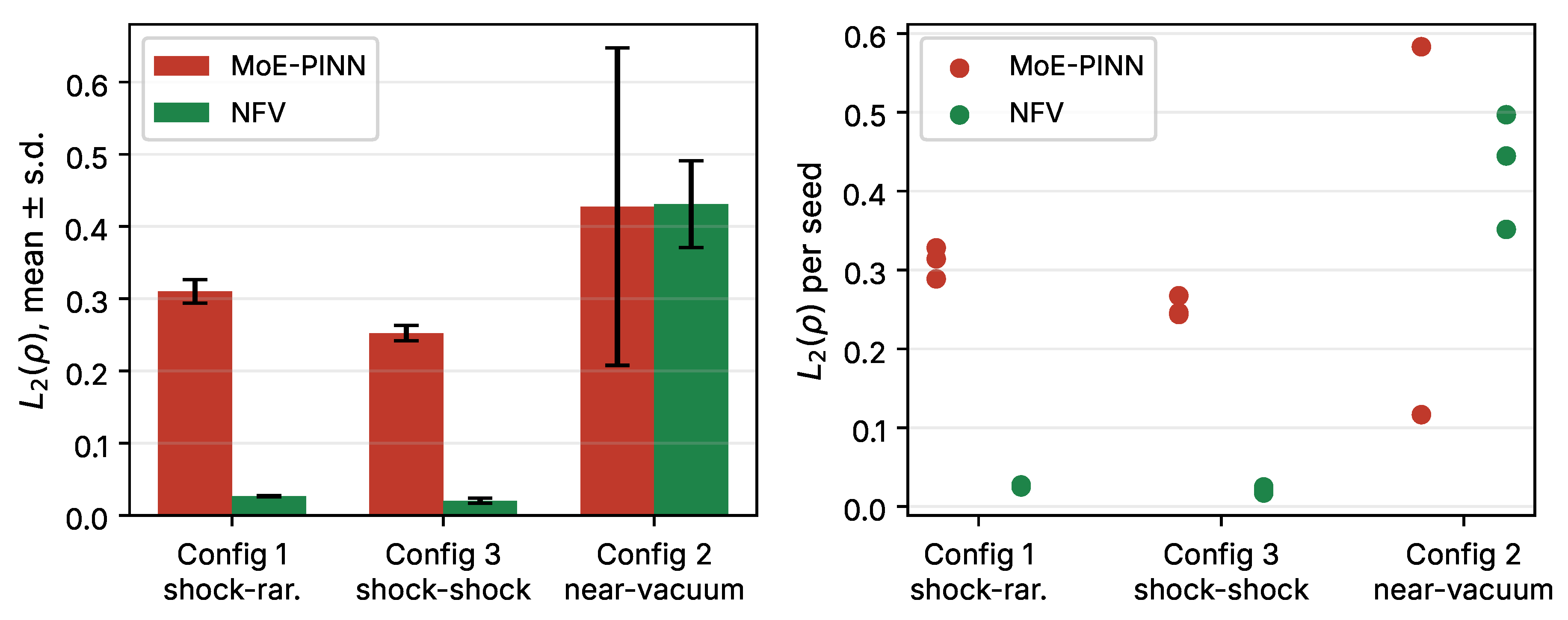
Figure 6. (Left): mean $L_2\left(\rho \right)$ error with standard-deviation bars, 3 seeds per method. (Right): individual seed values. On Configuration 2, the MoE-PINN seeds span 0.117–0.583 and those of NFV span 0.352–0.497.

(b) Size of the oscillations. On well-conditioned data, the MoE-PINN excursions stay below 6% for $\rho$ and 5% for u; its smoothing replaces overshoot. NFV overshoots by up to 8.8% in $\rho$ and 17.8% in u, and its velocity excursion reaches 931% near vacuum, where $u=\rho u/\rho$ is ill-conditioned (Figure 7). These oscillations do not crash the rollouts on well-conditioned data, but they are a substantive accuracy defect: a 10–18% velocity overshoot is too large for a solver used inside a coupled simulation. We regard them as acceptable only for qualitative wave-pattern prediction.

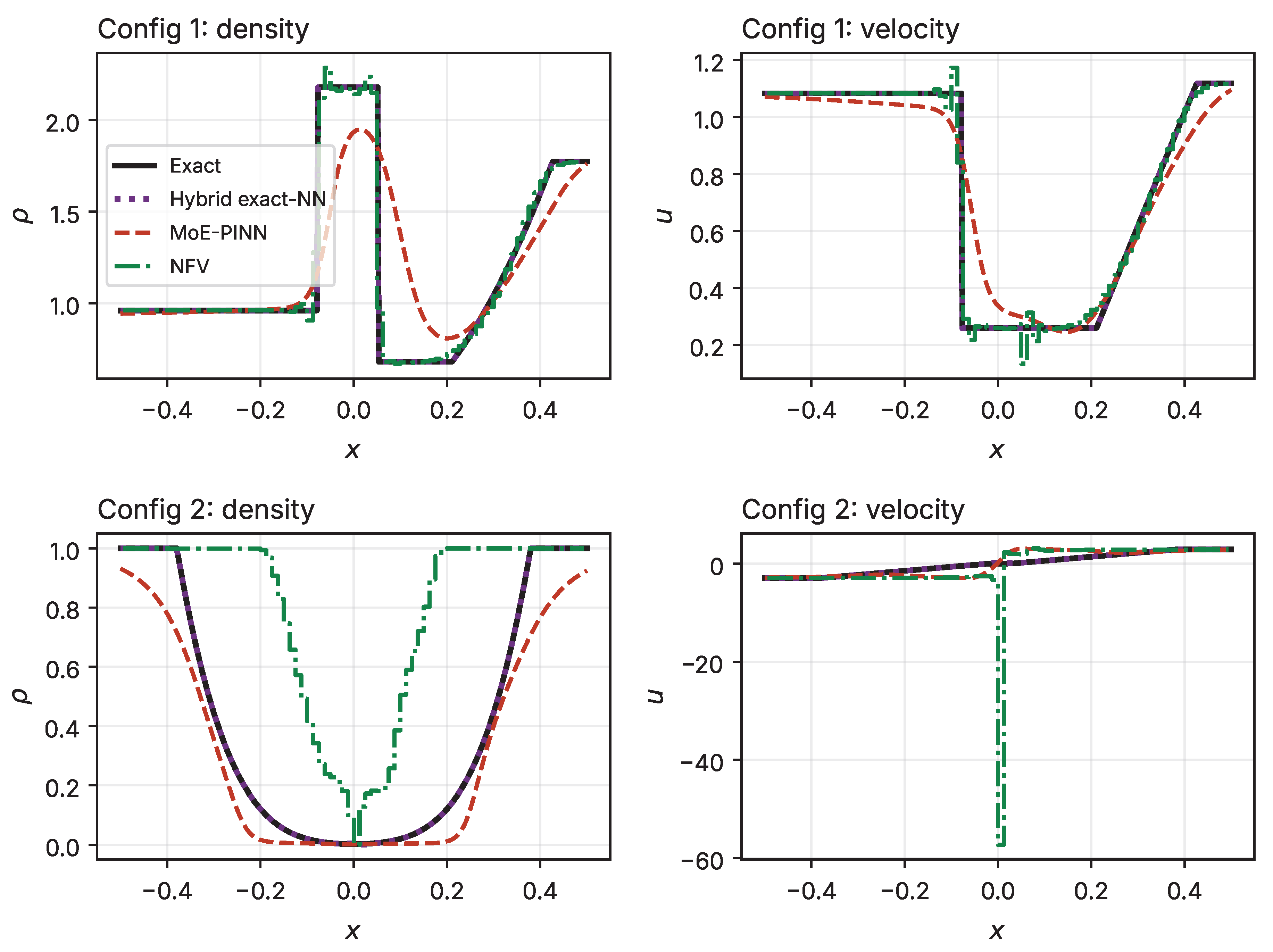
Figure 7. Representative profiles (seed 0) of Configurations 1 and 2 for all four methods. On Configuration 2, NFV seed 0 is the run with negative cell densities; its velocity spike at $x\approx 0$ results from dividing $\rho u$ by a near-zero density.

(c) Classical baselines also oscillate near contacts. Rusanov, which has no learned component, overshoots the velocity range by 29% on B and C and by 78% on E. To test whether the contact, where q jumps, can generate such excursions on its own, we computed a pure contact: $\rho$ jumps from 3.0 to 0.5, $u=u^{*}=-0.7899$ on both sides, and q is chosen so that $p+q$ is continuous. The exact solution translates the step with uniform velocity. The Rusanov, HLL and exact Godunov fluxes all generate a velocity error above 1.2 and a density dip toward zero at the contact, and the defect does not shrink between 100 and 800 cells (Section 8.5). Cell averaging of $\rho$ and $\rho q$ breaks the continuity of $p+q$ in the smeared cells by 0.62–0.84, independently of the grid, and the resulting momentum-flux imbalance drives the spurious velocity. The same mechanism produces pressure oscillations in multicomponent flow computations, where quasi-conservative updates of the advected variable remove it [21]; Section 8.5 adapts that remedy to this model.

(d) Limiting. None of the three neural methods uses a limiter or a monotonicity constraint. MoE-PINN enforces only $\rho >0$, through its output transform. The NFV conservative form admits standard positivity limiting, for example by blending ${\mathrm{\Phi }}_{\theta }$ with a positivity-preserving flux in cells that approach $\rho \le 0$ [25,26], and slope or flux limiting would damp its cell-scale oscillations. These devices act on the update, not on the network, so they cannot correct the inconsistency $\kappa$ of (16). The contact defect in (c) needs a different remedy, a contact-consistent update of q, for classical and learned conservative schemes alike; Section 8.5 tests one. Without such mechanisms, the oscillations in (b) and the near-vacuum failures in (a) remain a core limitation of the neural methods relative to positivity-preserving classical schemes.

6. A Hybrid Exact–Neural Scheme, Cross-Validated and Multi-Seed Evaluated

Section 3 and Section 4 each use a network globally: for the full solution field (MoE-PINN) or for the flux at every interface (NFV). This section tests a different approach, adapted from a hybrid HLLC-NN scheme [27] built for the Euler equations [20]. It keeps the exact solver of Section 2 at every interface and calls a trained network only where a cheap detector flags the solver’s root find as unreliable.

6.1. Failure Mode of the Exact Solver and the Detector

The root find for (11) fails, or converges outside $0<a\rho <1$, when the star densities approach vacuum or the singularity $a\rho \to 1$, and it has no root at all under (12). We build a detector for this failure:

$$\mathrm{flag}=(\mathtt{ier}\ne 1)\vee \parallel (F,G)\parallel >{10}^{-6}\vee \min ({\rho }_{-},{\rho }_{+})<{10}^{-3}\vee \max (a{\rho }_{-},a{\rho }_{+})>0.95,$$

(18)

where ier is the solver’s convergence flag and $(F,G)$ is the residual of (11). On a 400-case stress test concentrated near vacuum and near the singularity, the detector flags 193 cases (48.25%). Of the flagged cases, 30 have a star state and 163 generate a vacuum and have none, by Proposition 1 of Section 7; these 163 are all the vacuum cases of the test. On every unflagged case the solver returns the correct star state. Varying the residual tolerance and the density floor by factors of 0.2–5, and the singularity margin between 0.90 and 0.99, changes the flagged fraction to between 48.00% and 49.75%.

6.2. Cross-Validation Against Published Test Cases

Reference [14], co-authored by one of us, uses the same constants. Its two published test cases provide a check outside the self-consistency construction of Table 2.

The present solver reproduces Test 1’s ${\rho }_{-}$ to all six reported digits and agrees with the remaining three values to within 2.2–7.4% (Table 8). Both tests have the same wave pattern in both sources. We could not identify the cause of the remaining differences; the present values satisfy (11) to ${10}^{-12}$, and the closed form (6) removes any quadrature error from our side.

Table 8. Star densities for the two test cases of [14]: published values and the present solver (residual of (11) below $3\times {10}^{-12}$ in both cases).

Test	Quantity	Published [14]	Present	Difference
1 (shock–contact–shock)	${\rho }_{-}$	18.8009	18.8009	0.00%
	${\rho }_{+}$	18.450	18.8485	2.16%
2 (shock–contact–rarefaction)	${\rho }_{-}$	2.13	2.1799	2.34%
	${\rho }_{+}$	0.6330	0.6800	7.43%

6.3. Surrogate and Experimental Design

The surrogate predicts $({\rho }_{-},{\rho }_{+},u^{*})$ from $({\rho }_l,u_l,{\rho }_r,u_r,\Delta q)$ with a four-hidden-layer MLP (80 ReLU units per layer). We choose this architecture by analogy to [20], without validating alternatives for this model. We train it on 30,000 converged exact solutions (15,000 broad samples and 15,000 concentrated near vacuum and near the singularity), with the physics-based normalisation of [20]: per-sample scales, log-transformed densities and standardisation. We evaluate three configurations with three seeds (0, 1, 2) for MoE-PINN and NFV and five seeds (0–4) for the surrogate:

• Configuration 1: shock–contact–rarefaction (Test 2 of [14]); the detector does not fire, so the hybrid scheme equals the exact solution.
• Configuration 2: symmetric near-vacuum double rarefaction (${\rho }_l={\rho }_r=1$, $u_l=-2.92$, $u_r=2.92$, $q_l=q_r=0$); the star density is 0.00282. The solve started from $({\rho }_l,{\rho }_r)$ converges to negative densities, so the detector fires and the surrogate is used.
• Configuration 3: shock–contact–shock (${\rho }_l=1.5$, $u_l=0.8$, $q_l=0.5$, ${\rho }_r=1.0$, $u_r=-0.8$, $q_r=0.8$); the detector does not fire.

6.4. Results

On Configurations 1 and 3, the NFV error is about 12 times smaller than that of MoE-PINN, with small seed variance for both (Table 9, Figure 6). On Configuration 2, the hybrid scheme’s density-profile error is 0.00104 ± 0.00103 over five seeds, but this low value is misleading. The predicted star densities range over ${\rho }_{-}\in [0.00022,0.0040]$ and ${\rho }_{+}\in [0.0009,0.0223]$ against 0.00282, and the predicted $u^{*}$ ranges over $[0.152,0.422]$ against exactly 0. The profile error is small only because the true densities are themselves near zero.

Table 9. $L_2\left(\rho \right)$ error, mean ± standard deviation. MoE-PINN and NFV: 3 seeds (0–2). ^a Hybrid surrogate: 5 seeds (0–4). Bold: the lower of the NFV and MoE-PINN errors where their difference is statistically significant (paired t-test, $p<0.002$).

Config.	Hybrid Exact–NN	NFV	MoE-PINN
1 (shock–rarefaction)	0 (exact; detector silent)	$\mathbf{0.0265}\pm \mathbf{0.0011}$	$0.310\pm 0.016$
3 (shock–shock)	0 (exact; detector silent)	$\mathbf{0.0202}\pm \mathbf{0.0034}$	$0.252\pm 0.011$
2 (near-vacuum)	${0.00104\pm 0.00103 }^a$	$0.431\pm 0.060$	$0.428\pm 0.220$

Substituting the surrogate’s star states into the Riemann relations exposes the problem directly. On Configuration 2, the predicted $({\rho }_{-},{\rho }_{+})$ violate the velocity condition of (11) by 18–25% of the velocity scale $\sqrt{(p_l+p_r)/({\rho }_l+{\rho }_r)}$. On the 30 flagged stress cases that have a star state, the median relative star-density error is 10.9–25.3 (that is, 1090–2528%), and the median residual of (11) is 0.24–0.28. Between 11 and 21 of the 193 flagged predictions lie outside $0<a\rho <1$. The detector transfers; the surrogate does not yet provide reliable fallback states.

Table 10 gives two relative density errors. The floor-normalised metric divides by $\max \left(\right|{\rho }_{\mathrm{exact}}|,{10}^{-3})$ and is dominated by the floor as the exact density approaches zero; the NFV value of 9.5 does not mean a 950% error. Normalising by ${\rho }_0$ gives the error as a fraction of the initial density scale. Under this metric, the two methods are indistinguishable on Configuration 2 (0.168 ± 0.020 for NFV and 0.155 ± 0.077 for MoE-PINN, all three seeds), while the floor-normalised metric suggests a twelvefold difference.

Table 10. Relative density errors, mean ± standard deviation over 3 seeds. ${\rho }_0={\rho }_l+{\rho }_r$. Floor-normalised: mean of $|\rho -{\rho }_{\mathrm{exact}}|/\max (|{\rho }_{\mathrm{exact}}|,{10}^{-3})$.

Config.	Metric	NFV	MoE-PINN
1	$L_1\left(\rho \right)/{\rho }_0$	$0.0052\pm 0.0001$	$0.0642\pm 0.0046$
3	$L_1\left(\rho \right)/{\rho }_0$	$0.0030\pm 0.0004$	$0.0573\pm 0.0041$
2	$L_1\left(\rho \right)/{\rho }_0$	$0.168\pm 0.020$	$0.155\pm 0.077$
2	floor-normalised	$9.5\pm 1.6$	$0.8\pm 0.2$

We test the ranking with a paired t-test and a bootstrap 95% confidence interval on the mean difference in $L_2\left(\rho \right)$ (MoE-PINN minus NFV, $n=3$ seeds per configuration). Table 11 lists the results.

Table 11. Paired comparison of MoE-PINN and NFV, $L_2\left(\rho \right)$, 3 seeds.

Config.	Mean Difference	Paired-t p-Value	Bootstrap 95% CI
1	0.284	0.0017	(0.261, 0.301)
3	0.232	0.0015	(0.221, 0.250)
2 (near-vacuum)	−0.003	0.9874	(−0.380, 0.232)

With $n=3$, these tests have low power. The intervals for Configurations 1 and 3 exclude zero ($p=0.0017$ and $p=0.0015$). The interval for Configuration 2 spans zero ($p=0.9874$), so no ranking is supportable near vacuum.

Table 12 shows a cost structure that accuracy alone does not convey. MoE-PINN and NFV, following the per-problem training of [15,16], must be retrained for every new initial condition. The hybrid scheme trains once and reuses the surrogate. On the stress-test mix, where 48.25% of interfaces are flagged, the surrogate adds about 28% to the exact solver’s cost; on well-conditioned flows, it adds only the detector’s comparisons.

Table 12. Computational cost, single CPU thread. Per-call costs: one star-state solve or prediction; one MoE-PINN evaluation of a 200-point profile; one NFV flux evaluation over 81 interfaces (one time step). Training: range over all runs of this study. Per-call costs were measured together in one run; absolute values depend on the machine.

Method	Training Cost	Per-Call Cost	Reuse
Exact solver (hybrid Powell)	none	468 μs	any configuration
Exact solver (reduced, Section 7)	none	70 μs	any configuration, vacuum included
MoE-PINN	54–89 s per Riemann problem	852 μs per profile	none: retrained for each new initial state
NFV	5–21 s per Riemann problem	105 μs per step	none across new initial data
Hybrid exact–NN	about 23 s data generation plus 23 s training, once	468 μs, plus 267 μs when flagged	any future Riemann problem under this equation of state

6.5. What This Comparison Supports, and What It Does Not

On well-conditioned configurations (1, 3, A–D), NFV fits the exact solution 6–34 times more closely than a first-order scheme and 12 times more closely than MoE-PINN, with small seed variance. This advantage rests on supervised fitting of each target, and it shrinks to a factor near one on held-out data (Section 5.1). No ranking is supportable near vacuum: the seed spread exceeds the difference between methods, and both methods fail there in different ways, MoE-PINN by collapsing to a trivial state and NFV by leaving the admissible range. The hybrid scheme’s detector isolates the hard subset, including every vacuum case, but its surrogate returns star states that violate the Riemann relations.

The surrogate’s star-state errors call for a physics-constrained fallback with an explicit vacuum branch. Section 7 shows that a classical reduced solve provides exactly this, which leaves the learned fallback without a role on this model. The 2.2–7.4% differences from [14] remain unexplained.

7. Star-State Solvers as Constrained Residual Minimisation

Section 2, Section 3, Section 4, Section 5 and Section 6 leave three questions about the exact solver open. Is the 3-rarefaction relation of Remark 1 the one that the Riemann invariants require, and are the reported results unaffected by it? Do the reference star states, against which every method is measured, actually satisfy the Riemann relations? And can the solver’s failures near vacuum and near the singularity be removed without a learned fallback, which Section 6 showed to be unreliable? This section answers all three. It also asks how the star-state system (11) should be solved. We pose it as a constrained residual-minimisation problem, in which positivity and entropy admissibility enter as constraints, and we compare ten solution strategies.

The answer has two parts. First, the constraints decide the outcome. With positivity bounds alone, minimising the Rankine–Hugoniot residual returned a state with an expansion shock on 78.6% of the well-conditioned cases. With explicit entropy bounds on each wave, minimisation returned the correct star state on all 1237 solvable cases and identified all 163 vacuum cases. Second, eliminating the contact relation reduces the constrained problem to one monotone equation on a guaranteed bracket. This reduced form has the same reliability, needs a median of 14 residual evaluations, and costs about $1/116$ as much. Newton-type and least-squares solvers on the unconstrained or positivity-bounded residual failed on up to 34.9% of the well-conditioned cases.

7.1. The Constrained Residual-Minimisation Problem

Let $y=({\rho }_{-},{\rho }_{+})$, and let $R(y;U_l,U_r)\in {\mathbb{R}}^2$ collect the velocity relation and the contact relation of (11). The residual-minimisation formulation seeks

$$\underset{y\in \mathcal{A}}{\min }J\left(y\right)=\frac{1}{2}{∥R(y;U_l,U_r)∥}_2^2,\mathcal{A}=\{y:g_i\left(y\right)\le 0\},$$

(19)

where the constraints $g_i$ encode positivity, ${\rho }_{\pm }\ge 0$, the closure bound $a{\rho }_{\pm }<1$, and the entropy conditions of the two nonlinear waves. A star state is a point of $\mathcal{A}$ with $J=0$. For this model, the entropy conditions reduce to bounds on single densities.

Lemma 1.

Let $U^{*}\ne U_l$ lie on the 1-Hugoniot locus through $U_l$. The Lax conditions ${\lambda }_1\left(U^{*}\right)<S_1<{\lambda }_1\left(U_l\right)$ hold if and only if ${\rho }_{-}>{\rho }_l$. Let $U^{*}$ lie on the 1-integral curve through $U_l$. The fan is admissible, ${\lambda }_1\left(U_l\right)\le {\lambda }_1\left(U^{*}\right)$, if and only if ${\rho }_{-}\le {\rho }_l$. The same statements hold for field 3, with ${\rho }_{+}$, ${\rho }_r$ and the conditions ${\lambda }_3\left(U_r\right)<S_3<{\lambda }_3\left(U^{*}\right)$ and ${\lambda }_3\left(U^{*}\right)\le {\lambda }_3\left(U_r\right)$.

Proof. 

By Table 1, q is a Riemann invariant of fields 1 and 3, so it is constant across these waves. The mass and momentum equations of (1) then form the isentropic gas-dynamics system with pressure p. In specific volume $\tau =1/\rho$, $d^{2}p/d{\tau }^2={\rho }^3(\rho p^{″}+2p^{\prime })>0$ by (3). For such a pressure law, the Lax-admissible part of the Hugoniot locus is its compressive branch, ${\rho }_{*}>{\rho }_K$ [28,29]. Along the integral curve, $d{\lambda }_1/d\rho =-(\sigma +\rho {\sigma }^{\prime })/\rho <0$, because $\rho {\sigma }^{\prime }=\rho p^{″}/\left(2\sigma \right)>0$. Hence ${\lambda }_1$ increases as $\rho$ decreases, which proves the fan statement. Field 3 follows by symmetry. □

Lemma 1 turns each entropy condition into a bound on one star density. We compare three formulations of (19). On each side, the residual uses either the Hugoniot relation (S), continued through $U_K$ as $u_{-}=u_l-\mathrm{sgn}({\rho }_{-}-{\rho }_l)\sqrt{[p\left({\rho }_{-}\right)-p\left({\rho }_l\right)](1/{\rho }_l-1/{\rho }_{-})}$, or the Riemann-invariant relation (R) of (7) or (8).

• RH residual, positivity bounds. Both sides use the Hugoniot relation, and $\mathcal{A}$ contains only ${\rho }_{\pm }\ge 0$. No constraint enforces entropy admissibility.
• RH residual + Lax constraints. As above, with the Lax bounds ${\rho }_{-}\ge {\rho }_l$ and ${\rho }_{+}\ge {\rho }_r$ of Lemma 1 added.
• Wave-configuration residual + entropy bounds (RM-E). For each of the four wave configurations $w=(w_l,w_r)$, with $w_l,w_r\in \{\mathrm{S},\mathrm{R}\}$, the residual $R_w$ uses the relation of w on each side, and ${\mathcal{A}}_w$ imposes Lemma 1’s bound for that wave: ${\rho }_{-}\ge {\rho }_l$ for a 1-shock, ${\rho }_{-}\le {\rho }_l$ for a 1-rarefaction, and likewise on the right. The solver accepts the configuration whose minimum is zero. If no configuration reaches zero, it evaluates the velocity residual at the boundary point of $\mathcal{A}$ where the contact relation holds and the density on the low-pressure side vanishes. A non-positive value proves a vacuum (Corollary 1 below); a positive value is reported as a failure.

• All three solve bound-constrained least-squares problems with TRF [30]. The unknowns are $z_{\pm }=\mathrm{\Phi }\left({\rho }_{\pm }\right)$. Because $\mathrm{\Phi }$ increases from $\mathrm{\Phi }\left(0\right)=0$ to $+\infty$ as $a\rho \to 1$, positivity becomes $z\ge 0$, the singular bound drops out, and the residual stays well conditioned near vacuum. The S and R bounds overlap by a relative ${10}^{-6}$ at ${\rho }_K$, so that a weak wave lies inside a box. The Hugoniot locus and the integral curve agree to second order at $U_K$, so their relations differ by $O\left(\right|{\rho }_{*}-{\rho }_K{|}^3)$, at most ${10}^{-18}$ in relative terms, inside the overlap. Each problem starts from $({\rho }_l,{\rho }_r)$ projected into its box. Inside a Godunov scheme it starts instead from the previous step’s star state at the same interface, and the solver tries that state’s configuration first. We accept a minimiser if its residual, scaled by the velocity and pressure scales of the data, is below ${10}^{-8}$.

7.2. A Reduced Formulation with Existence and Uniqueness

The contact relation in (11), $p\left({\rho }_{-}\right)-p\left({\rho }_{+}\right)=\Delta q$ with $\Delta q=q_r-q_l$, fixes one star density once the other is known, because p is strictly increasing with the explicit inverse

$$p^{-1}\left(P\right)={\displaystyle \frac{s}{1+as}},s={(P/A)}^{1/\gamma }.$$

(20)

We take as the single unknown the star density s on the low-pressure side of the contact: $s={\rho }_{+}$ and ${\rho }_{-}=p^{-1}(p\left(s\right)+\Delta q)$ if $\Delta q>0$; otherwise $s={\rho }_{-}$ and ${\rho }_{+}=p^{-1}(p\left(s\right)-\Delta q)$. The map then adds a non-negative quantity, so it involves no cancellation as $s\to 0$. Define

$$f\left(s\right)=u_{-}\left({\rho }_{-}\left(s\right)\right)-u_{+}\left({\rho }_{+}\left(s\right)\right),0\le s<1/a,$$

(21)

where $u_{-}$ is given by (7) or (10) and $u_{+}$ by (8) or (10).

Proposition 1.

Let $0<{\rho }_l,{\rho }_r<1/a$. Then f is continuous and strictly decreasing on $[0,1/a)$, and $f\left(s\right)\to -\infty$ as $s\to 1/a$. Hence system (11) has a solution with $0<{\rho }_{\pm }<1/a$ if and only if $f\left(0\right)>0$, and that solution is unique. If $f\left(0\right)\le 0$, no star state with positive densities exists and the Riemann solution contains a vacuum. For $\Delta q=0$, the condition $f\left(0\right)>0$ reduces to $u_r-u_l<\mathrm{\Phi }\left({\rho }_l\right)+\mathrm{\Phi }\left({\rho }_r\right)$, the complement of (12).

Proof. 

On the rarefaction branch, $d{u}_{-}/d\rho =-\sigma \left(\rho \right)/\rho <0$. On the shock branch, $u_{-}=u_l-\sqrt{g}$ with $g=[p\left(\rho \right)-p\left({\rho }_l\right)](1/{\rho }_l-1/\rho )$, a product of two positive, strictly increasing factors for $\rho >{\rho }_l$. Both branches equal $u_l$ at $\rho ={\rho }_l$, so $u_{-}$ is continuous and strictly decreasing; the same argument shows that $u_{+}$ is continuous and strictly increasing. Both ${\rho }_{-}\left(s\right)$ and ${\rho }_{+}\left(s\right)$ increase strictly with s, because p and $p^{-1}$ do. Hence f is strictly decreasing. As $s\to 1/a$, both star densities tend to $1/a$, p diverges, and the shock branches give $u_{-}\to -\infty$ and $u_{+}\to +\infty$. The intermediate value theorem then gives a root if and only if $f\left(0\right)>0$, and strict monotonicity makes it unique. At $s=0$ with $\Delta q=0$, both star densities vanish and $f\left(0\right)=u_l+\mathrm{\Phi }\left({\rho }_l\right)-u_r+\mathrm{\Phi }\left({\rho }_r\right)$. □

The branch functions select a shock exactly when the star density exceeds the far-field density. By Lemma 1, this choice satisfies the Lax entropy conditions, so the unique root is the entropy solution. Positivity is built into the unknown’s domain. The reduced solve therefore imposes both admissibility constraints of (19) without penalty terms. We solve $f\left(s\right)=0$ with Brent’s method [31] on $[0,s_{\mathrm{hi}}]$, where $s_{\mathrm{hi}}=(1-\delta )/a$ and $\delta ={10}^{-2},{10}^{-4},\dots$ until $f\left(s_{\mathrm{hi}}\right)<0$. The bracket always exists by Proposition 1, so the iteration cannot diverge.

Corollary 1

(one-dimensional residual minimisation). Restrict problem (19), with the entropy bounds of Lemma 1, to the contact manifold $R_2=0$. On it, s parametrises the admissible set as $0\le s<1/a$, and $J=\frac{1}{2}f{\left(s\right)}^2$. Because $f^{\prime }<0$, the derivative $J^{\prime }=f{f}^{\prime }$ vanishes only where $f=0$. If $f\left(0\right)>0$, the unique minimiser is the root of f, with $J=0$. If $f\left(0\right)\le 0$, J increases on $[0,1/a)$, and the unique minimiser is the positivity boundary $s=0$, with $J\left(0\right)=\frac{1}{2}f{\left(0\right)}^2\ge 0$. In that case the minimiser lies on the boundary of $\mathcal{A}$, and the Riemann solution contains a vacuum.

The reduced solve is therefore problem (19) with the contact relation eliminated, and the bracketed root search is its exact one-dimensional minimisation. The elimination is possible because the contact field is linearly degenerate: its relation $p\left({\rho }_{-}\right)-p\left({\rho }_{+}\right)=\Delta q$ is explicit and monotone. The vacuum test of RM-E evaluates the same boundary value $f\left(0\right)$.

Proposition 1 also settles the sign question of Remark 1. Its proof needs $u_{+}$ to increase with ${\rho }_{+}$ on both branches, and relation (8) gives $d{u}_{+}/d{\rho }_{+}=\sigma /{\rho }_{+}>0$. The sign-flipped candidate would give $d{u}_{+}/d{\rho }_{+}=-\sigma /{\rho }_{+}<0$ on the rarefaction branch, so f would lose its monotonicity and the root its uniqueness. The reduced solve, which shares no code path with the solver of Section 2, reproduces the star states of Table 2, of Configurations 1–3 and of both test cases of [14] to a relative difference of at most $9\times {10}^{-13}$. Every result of Section 2, Section 3, Section 4, Section 5 and Section 6 therefore stands as reported.

Proposition 1 also corrects the vacuum count of the stress test in Section 6. Criterion (12) assumes $\Delta q=0$ and flags 39 of the 400 cases as vacuum-generating; the general condition $f\left(0\right)\le 0$ applies to 163.

7.3. Six Strategies on the Branch-Function Residual

We compare the reduced solve with six strategies that work directly on the two-variable residual $R({\rho }_{-},{\rho }_{+})$ of (11): Newton–Raphson with a finite-difference Jacobian; damped Newton with backtracking and projection into $0<\rho <1/a$; the MINPACK hybrid Powell method [32], used in Section 2, Section 3, Section 4, Section 5 and Section 6; Broyden’s quasi-Newton method [33]; Levenberg–Marquardt least squares [34,35]; and the bound-constrained least-squares problem

$$\underset{{\rho }_{\pm }}{\min }\frac{1}{2}{\parallel R({\rho }_{-},{\rho }_{+})\parallel }_2^2\mathrm{subject}\mathrm{to}0<{\rho }_{\pm }<1/a,$$

(22)

solved with a trust-region reflective (TRF) method [30]. Problem (22) is (19) with positivity and singularity bounds on the branch-function residual. The branch functions already select the admissible wave, so (22) needs no separate entropy constraint; Section 7.4 shows what happens when the residual does not select it. All strategies start from $({\rho }_l,{\rho }_r)$, as a Godunov scheme would. The four unbounded methods evaluate R with the densities clipped into the domain as in our original implementation. We count an output as correct if it lies in $0<{\rho }_{\pm }<1/a$ and satisfies (11) to a relative residual below ${10}^{-8}$, scaled by the velocity and pressure scales of the data. By Proposition 1, such an output is the unique root. The test sets are 1000 random well-conditioned cases (${\rho }_{l,r}\in [0.1,10]$, $u_{l,r}\in [-2,2]$, $\Delta q\in [-2,2]$, all with a star state) and the 400-case stress test of Section 6, of which 237 have a star state (largest $a{\rho }_{\pm }$ = 0.938) and 163 generate a vacuum.

Three results follow from Table 13. First, every unbounded method converges to inadmissible states: Newton–Raphson on 34.9% of the well-conditioned cases, Levenberg–Marquardt on 14.6%, Broyden on 10.5% and hybrid Powell on 9.3%. Clipping the densities inside R creates spurious zeros at negative densities, where the clipped residual vanishes; Configuration 2, for example, converges to ${\rho }_{\pm }=-2.344$ from its natural starting point. A convergence flag is therefore no evidence of a physical star state. Second, the two bounded methods never return inadmissible states, but they stop at admissible non-roots (damped Newton on 16 and TRF on 2 solvable stress cases). On every vacuum case they return a bounded minimiser with a non-zero residual, so the residual must be checked after the solve. TRF is also the most expensive method, at 4.2 ms per solve. Third, the reduced solve is correct on every solvable case, identifies every vacuum case, reaches a relative residual of at most 7 × 10⁻¹⁵, and needs at most 32 residual evaluations, at a median of 66 μs.

Table 13. Star-state solvers, started from $({\rho }_l,{\rho }_r)$. Well-conditioned: 1000 cases with a star state (% correct, inadmissible output, admissible non-root). Stress: 400 cases; correct/inadmissible/non-root on the 237 cases with a star state, and the outcome on the 163 vacuum cases. Cost: median residual evaluations and median time per solve on the well-conditioned set (single CPU thread). Bold: the reduced solver of Proposition 1, the only method correct on every case with a star state that also identifies every vacuum case.

	Well-Conditioned (%)			Stress Test		Cost
Method	Correct	Inadm.	Non-Root	with Star State	Vacuum Cases	Evals	μs
Newton–Raphson	65.1	34.9	0.0	154/82/1	163 inadm.	18	247
damped Newton (bounds)	99.7	0.0	0.3	221/0/16	163 non-root	27	640
hybrid Powell (fsolve)	90.7	9.3	0.0	208/28/1	151 inadm., 12 non-root	19	154
Broyden (quasi-Newton)	89.5	10.5	0.0	181/53/3	163 inadm.	16	1740
Levenberg–Marquardt	85.4	14.6	0.0	179/57/1	163 inadm.	24	1647
bound-constrained LS (TRF)	99.7	0.0	0.3	235/0/2	163 non-root	25	4200
reduced bracketed (Brent)	100.0	0.0	0.0	237/0/0	163 identified	14	66

The reduced solve also removes the need for the learned fallback of Section 6. Of the 193 cases the detector flags, it solves all 30 cases with a star state and proves the vacuum in the other 163, without training data. Its median cost of 70 μs is below the hybrid Powell solve alone (468 μs, Table 12), even before the surrogate’s 267 μs.

7.4. Entropy Constraints in the Minimisation

Table 14 gives three results. First, the Rankine–Hugoniot residual with positivity bounds alone has a zero in every case, but that zero is the entropy solution only when both waves are shocks. Of the 1000 well-conditioned cases, 207 contain two shocks. On the other 793, minimisation converges to a root with an expansion shock in all but seven, which have weak rarefactions; overall, 78.6% of the outputs violate the entropy condition. On all 163 vacuum cases, it returns a spurious root because expansion shocks can close any velocity gap. Each such root satisfies its Rankine–Hugoniot relations to machine precision, so a residual check cannot reject it.

Table 14. Residual minimisation with and without entropy constraints (Section 7.1), on the test sets of Table 13. Well-conditioned (%): correct star state; root with an expansion shock (entropy-violating); non-zero minimum. Stress: correct/entropy-violating/non-zero on the 237 cases with a star state, and vacuum identified/spurious root/non-zero minimum on the 163 vacuum cases. Cost: median residual evaluations and median time per solve on the well-conditioned set. Bold: the reduced solver of Proposition 1, which matches the reliability of RM-E at about 1% of its run time.

	Well-Conditioned (%)			Stress Test		Cost
Formulation	Correct	Entropy-Viol.	Non-Zero	with Star State	Vacuum Cases	Evals	ms
RH, positivity only	21.4	78.6	0.0	53/184/0	0/163/0	22	2.1
RH + Lax bounds	20.7	0.0	79.3	49/0/188	0/0/163	30	3.1
RM-E, entropy bounds	100.0	0.0	0.0	237/0/0	163/0/0	76	7.7
reduced (Prop. 1)	100.0	0.0	0.0	237/0/0	163/0/0	14	0.07

Second, the Lax constraints remove every entropy-violating root, but the constrained problem then has no zero whenever a rarefaction is present (79.3% of the well-conditioned cases). Its minimum lies on the constraint ${\rho }_{*}={\rho }_K$ with a positive residual. Lax constraints can detect a rarefaction, but they cannot represent one.

Third, the wave-configuration formulation with entropy bounds returns the correct star state on all 1000 well-conditioned and all 237 solvable stress cases, and it identifies all 163 vacuum cases. We check every accepted state against the Lax conditions in their characteristic form, with the computed shock speeds; none violates them. RM-E solves 2.39 bound-constrained problems per case on average (3.16 on the stress set), at a median of 76 residual evaluations and 7.7 ms. That cost is about 116 times that of the reduced solve. The comparison isolates the cause: all three formulations use the same minimisation algorithm, and only their constraints differ. The entropy constraints, not the algorithm, decide whether residual minimisation returns the physical star state.

8. Godunov Schemes Built on the Star-State Solvers

Section 5.3 finds that the neural methods leave the admissible range near vacuum and oscillate near steep features, and that classical conservative schemes also oscillate at contacts. This section asks whether a classical scheme built on a solver whose star states are always admissible stays in the admissible range, satisfies the entropy condition and converges, and whether the contact defect can be repaired. It measures how the choice of Riemann solver affects the accuracy, robustness and entropy consistency of a first-order Godunov scheme. We compare a Godunov scheme whose interface flux uses the exact Riemann solution from the reduced solve (“Godunov”), the same scheme with the Powell or TRF solve and a Rusanov fallback when that solve fails, the same scheme driven by the residual-minimisation solvers of Section 7.1 (Section 8.4), and the approximate HLL [36] (with Davis wave-speed estimates [37]) and Rusanov fluxes. The exact flux samples the self-similar solution at $x/t=0$, including the two-rarefaction vacuum solution when Proposition 1 detects one. All schemes use 100–800 cells, CFL 0.5 and transmissive boundaries. On well-conditioned data, the exact-flux scheme is the most accurate of the three conservative fluxes, needs no fallback on any test, and stays positive. Driven by entropy-constrained residual minimisation, the same scheme gives the same solution; without the entropy constraints, it forms expansion shocks.

8.1. Accuracy and Convergence

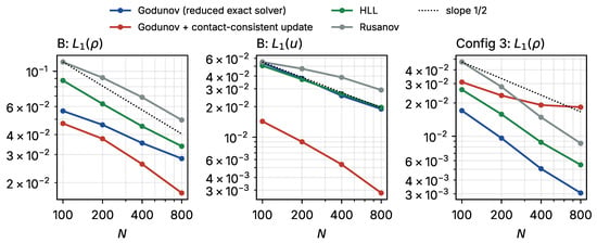
Among the three conservative fluxes, Godunov with the exact solver gives the smallest density error on every configuration (Table 15). Its error is 1.4–2.8 times smaller than that of Rusanov and 1.01–1.80 times smaller than that of HLL. All schemes converge at the reduced rates typical of first-order schemes with discontinuities: the observed order of $L_1\left(\rho \right)$ lies between 0.23 and 0.84 (Figure 8). The exact flux costs about 1.6 times as much as Rusanov per run in our implementation.

Table 15. $L_1$ errors at $N=800$ against exact cell averages, and the observed order of convergence (EOC) of $L_1\left(\rho \right)$, fitted over $N=100$–800. QC: Godunov with the contact-consistent update (24). Bold: smallest $L_1\left(\rho \right)$. All schemes are deterministic (one run each).

	${\mathit{L}}_1\left(\mathit{\rho }\right)$				${\mathit{L}}_1\left(\mathit{u}\right)$				EOC of ${\mathit{L}}_1\left(\mathit{\rho }\right)$
Config.	Godunov	QC	HLL	Rusanov	Godunov	QC	HLL	Rusanov	Godunov	Rusanov
A	0.0114	0.0182	0.0120	0.0201	0.0026	0.0052	0.0026	0.0064	0.45	0.56
B	0.0283	0.0172	0.0338	0.0494	0.0189	0.0028	0.0197	0.0292	0.34	0.40
C	0.0282	0.0172	0.0338	0.0494	0.0189	0.0028	0.0197	0.0292	0.33	0.40
D	0.0040	0.0056	0.0040	0.0057	0.0038	0.0050	0.0038	0.0056	0.54	0.56
E	0.0408	0.0284	0.0447	0.0555	0.0151	0.0038	0.0165	0.0218	0.23	0.33
Config. 1	0.0253	0.0383	0.0417	0.0451	0.0106	0.0148	0.0163	0.0173	0.51	0.47
Config. 3	0.0031	0.0183	0.0055	0.0086	0.0014	0.0050	0.0018	0.0035	0.84	0.83

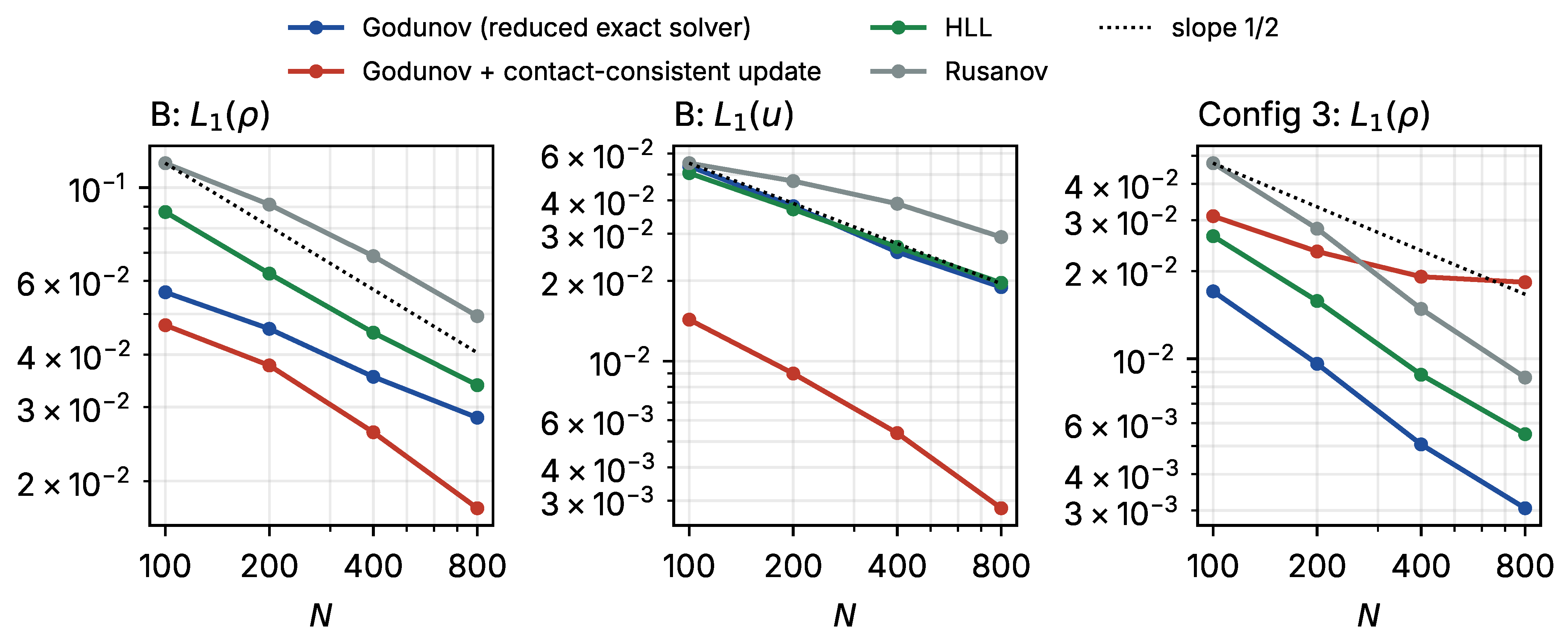
Figure 8. Grid convergence of the $L_1$ errors for Configuration B (density and velocity) and Configuration 3 (density).

8.2. Robustness near Vacuum and near the Singularity

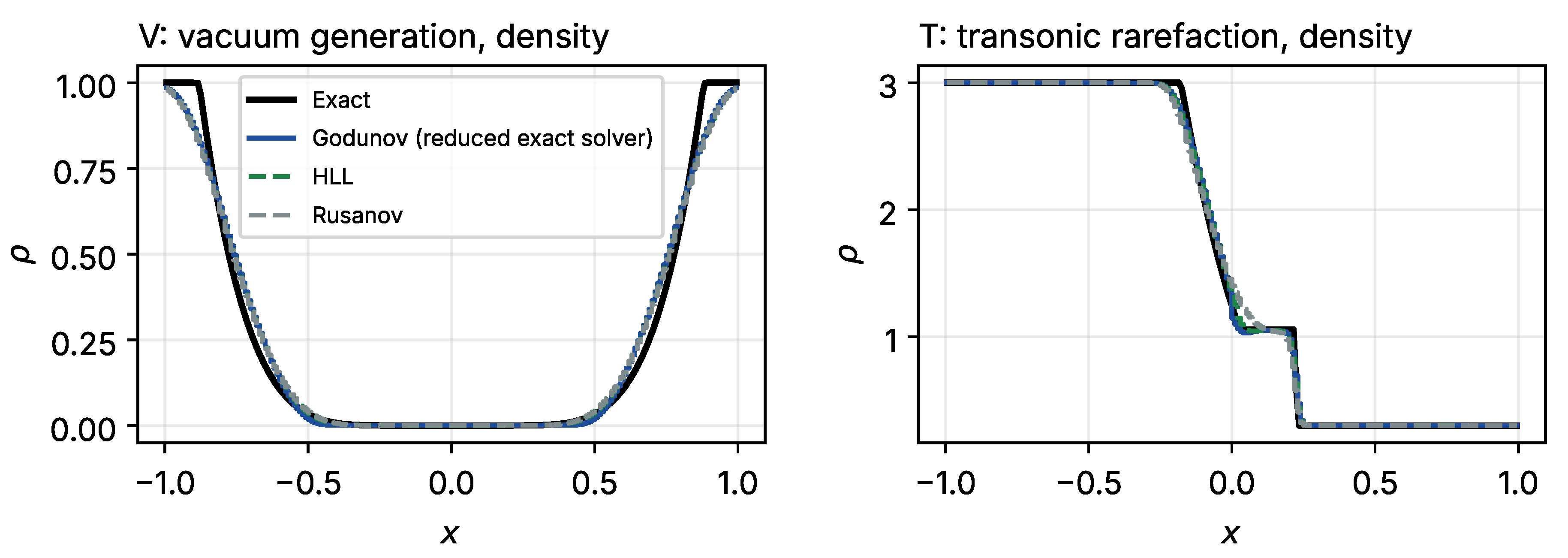
We run four demanding problems at $N=200$: Configuration 2 (near vacuum); V, which generates a vacuum (${\rho }_{l,r}=1$, $u_{l,r}=\mp 5$, $q\equiv 0$); S, whose star density reaches $a\rho =0.908$ (${\rho }_{l,r}=15$, $u_{l,r}=\pm 6$, $T=0.05$); and T, a transonic rarefaction (${\rho }_l=3$, ${\rho }_r=0.3$, $u\equiv 0$, $q\equiv 0$).

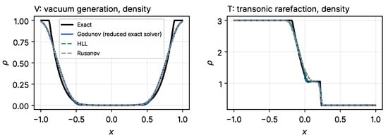
The reduced solver needs no fallback on any test, including the vacuum problem, where the exact flux samples the two-rarefaction vacuum solution (Table 16, Figure 9). The Powell solve fails on 0.1% of the interface problems of Configuration 2 and on 1.1% of those of V, and the scheme runs only because of the Rusanov fallback. The bound-constrained TRF solve, started from $({\rho }_l,{\rho }_r)$ at every step, fails on 6.9% of them and takes 831 s against 2.1 s; Section 8.4 shows that a warm start removes most of this cost. No scheme produces a negative density or reaches $a\rho \ge 1$. Near the singularity (S), the exact flux is 3.6 times more accurate than Rusanov and 2.6 times more accurate than HLL. Near vacuum, all fluxes give similar density errors because first-order smearing dominates.

Table 16. Robustness at $N=200$. Fallbacks: interface Riemann problems whose solve failed and fell back to the Rusanov flux, over all distinct interface solves. ${\rho }_{\min }$ and $\max a\rho$ over all cells and steps; time in seconds for the whole run.

Test	Scheme	${\mathit{L}}_1\left(\mathit{\rho }\right)$	Fallbacks	${\mathit{\rho }}_{\min }$	$\max \mathit{a}\mathit{\rho }$	Time (s)
Config. 2 (near vacuum)	Godunov, reduced	0.0269	0/19,118	0	0.035	2.1
	Godunov, Powell + fallback	0.0252	24/19,739	3.8 $\times {10}^{-5}$	0.035	4.3
	Godunov, TRF (cold) + fallback	0.0267	1368/19,710	0	0.035	831.1
	HLL	0.0249	–	0.002	0.035	0.4
	Rusanov	0.0251	–	0.0003	0.035	0.6
V (vacuum)	Godunov, reduced	0.0289	0/21,966	6.2 $\times {10}^{-13}$	0.035	3.1
	Godunov, Powell + fallback	0.0283	283/24,661	8.1 $\times {10}^{-7}$	0.035	5.3
	HLL	0.0283	–	1 $\times {10}^{-6}$	0.035	0.5
	Rusanov	0.0286	–	1.5 $\times {10}^{-12}$	0.035	0.7
S (near singular)	Godunov, reduced	0.0186	0/12,499	15	0.910	2.1
	Godunov, Powell + fallback	0.0190	4/12,570	15	0.910	3.2
	HLL	0.0480	–	15	0.908	0.7
	Rusanov	0.0679	–	15	0.908	1.7
T (transonic)	Godunov, reduced	0.0164	0/2967	0.3	0.105	0.4
	Godunov, Powell + fallback	0.0164	0/2958	0.3	0.105	0.6
	HLL	0.0173	–	0.3	0.105	0.3
	Rusanov	0.0249	–	0.3	0.105	0.2

Figure 9. Density at $N=200$ for the vacuum problem V ($t=0.15$) and the transonic rarefaction T ($t=0.15$).

8.3. Entropy Consistency

Every interface solution of the exact solver satisfies the Lax conditions by construction (Proposition 1). We checked the discrete solution on the transonic rarefaction T, where schemes without entropy fixes can form expansion shocks at the sonic point.

The Godunov scheme converges on T with order 0.76, like HLL (0.77) and faster than Rusanov (0.66), and it has the smallest error at every resolution (Table 17). Its jump ratio stays between 1.6 and 2.1 as N grows eightfold, so the largest jump inside the fan shrinks like $1/N$: the scheme shows the known first-order kink at the sonic point but no expansion shock.

Table 17. Transonic rarefaction T. Jump ratio: largest density jump between neighbouring cells inside the fan, divided by the largest jump between neighbouring exact cell averages; an expansion shock would make this ratio grow like N.

	Godunov		HLL		Rusanov
$\mathit{N}$	${\mathit{L}}_{\mathbf{1}}\left(\mathit{\rho }\right)$	Jump Ratio	${\mathit{L}}_{\mathbf{1}}\left(\mathit{\rho }\right)$	Jump Ratio	${\mathit{L}}_{\mathbf{1}}\left(\mathit{\rho }\right)$	Jump Ratio
100	0.0282	1.64	0.0302	0.63	0.0393	0.58
200	0.0164	1.88	0.0173	0.85	0.0249	0.66
400	0.0097	2.05	0.0103	0.96	0.0161	0.73
800	0.0059	2.14	0.0060	0.95	0.0099	0.78

8.4. Godunov Schemes Driven by Residual Minimisation

We embedded three residual-minimisation solvers in the same Godunov scheme and ran all eleven tests of Table 15 and Table 16 at $N=200$: the entropy-constrained RM-E; TRF on the branch-function residual (22), now warm-started from the previous step’s star state at the same interface; and the RH residual with positivity bounds only. When a solve returns a non-zero residual, the interface uses the Rusanov flux. For the RH solver, the flux samples each wave as a jump that moves at its Rankine–Hugoniot speed, which is the two-shock approximation [38].

RM-E needs no fallback on any of the eleven tests, 93,015 interface solves in total. Its solution matches the reduced Godunov solution to a relative difference of at most 8 × 10⁻¹⁰ (Table 18). The accuracy, robustness and entropy results of Section 8.1, Section 8.2 and Section 8.3 therefore hold for the RM-E scheme. The warm start cuts the work per solve: RM-E solves at most 1.32 bound-constrained problems per interface, against 2.39 from a cold start (Table 14). The cost remains high, at 44–66 times the run time of the reduced solve.

Table 18. Godunov schemes whose interface solver is a residual-minimisation method, $N=200$. RM-E: Rusanov fallbacks (fallb.); maximum relative difference from the Godunov solution with the reduced solve, over all cells and variables; mean bound-constrained problems per interface solve (probl.); run time. Reduced: run time of the Godunov scheme with the reduced solve. TRF, warm start: fallbacks and run time. RH, no entropy constraint: share of interface solves whose root contains an expansion shock, and $L_1\left(\rho \right)$ relative to the reduced Godunov scheme.

	Godunov, RM-E				Reduced	TRF, Warm Start		RH, No Entropy Constr.
Test	Fallb.	Max Diff	Probl.	Time (s)	Time (s)	Fallb.	Time (s)	Exp. sh. (%)	${\mathit{L}}_{\mathbf{1}}\left(\mathit{\rho }\right)$ Ratio
A	0	$6\times {10}^{-12}$	1.01	17	0.32	0	4	2	1.00
B	0	$7\times {10}^{-11}$	1.05	24	0.38	13	6	48	1.17
C	0	$4\times {10}^{-11}$	1.04	25	0.50	13	6	47	1.19
D	0	$8\times {10}^{-10}$	1.03	16	0.29	0	4	79	1.04
E	0	$2\times {10}^{-11}$	1.05	14	0.25	0	3	60	1.00
Config. 1	0	$9\times {10}^{-12}$	1.03	57	1.09	0	17	73	1.00
Config. 3	0	$8\times {10}^{-10}$	1.05	28	0.42	0	6	5	1.00
Config. 2	0	$2\times {10}^{-12}$	1.02	67	1.29	140	27	89	1.00
V	0	$3\times {10}^{-12}$	1.01	74	1.68	177	36	89	1.00
S	0	$6\times {10}^{-10}$	1.32	67	1.17	0	17	58	1.00
T	0	$6\times {10}^{-10}$	1.03	14	0.24	0	3	47	1.24

The warm start also helps TRF on the branch-function residual. On Configuration 2 its failures fall from 6.9% of interface solves to 0.7%, and its run time from 831 s to 27 s. It still fails near vacuum (140 fallbacks on Configuration 2 and 177 on V) and at the spurious near-vacuum states of the contact defect in B and C (13 each). Each fallback replaces the exact flux by the Rusanov flux, so on these four tests, the solution departs from the exact-flux solution by 0.13–0.43 in relative terms.

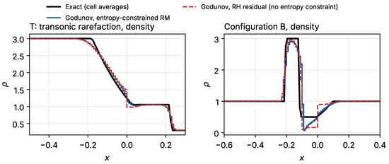
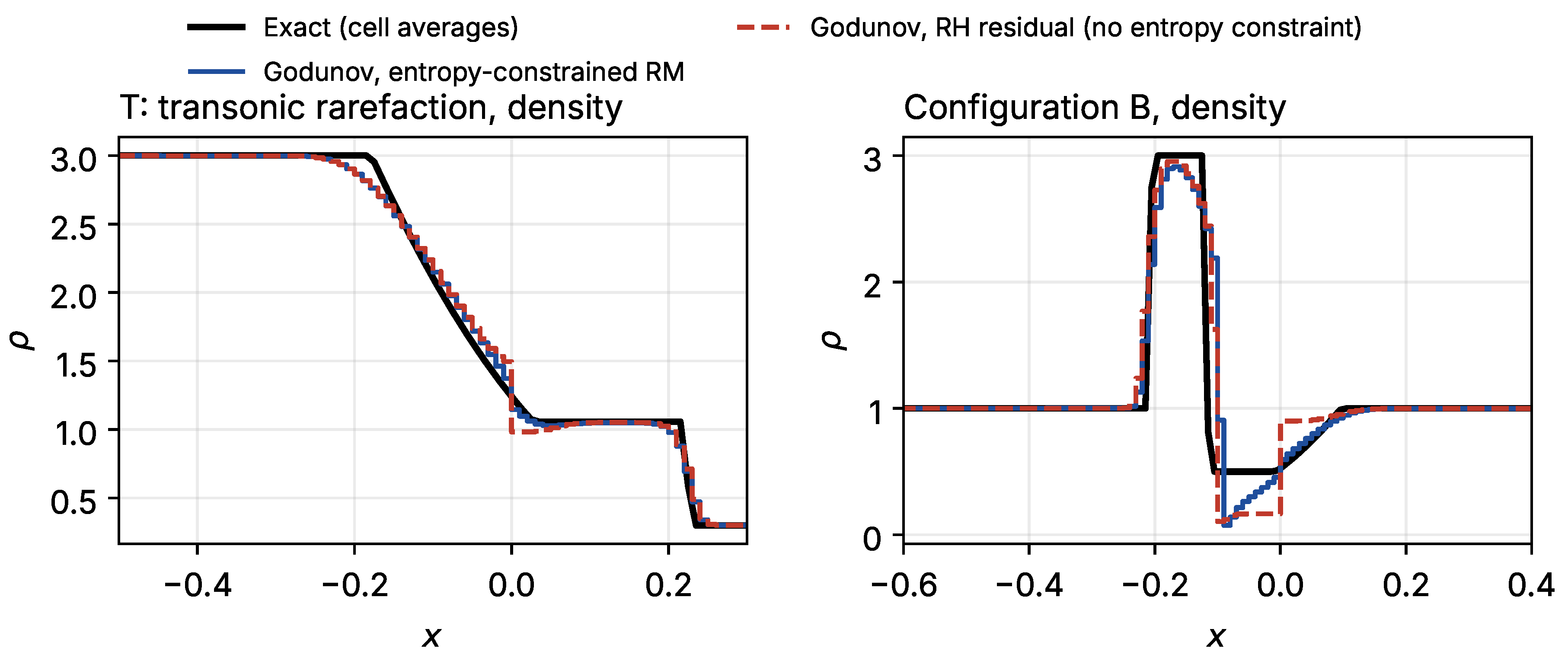
Without entropy constraints, the scheme forms expansion shocks. The RH residual chooses an expansion shock in 2–89% of the interface solves. Where the rarefactions are weak or move away from the interface, the two-shock flux stays within 4% of the exact flux in $L_1\left(\rho \right)$. Next to the contact in B and C, it raises $L_1\left(\rho \right)$ by a factor of 1.17–1.19, and on B it raises $L_1\left(u\right)$ by a factor of 2.1. At the sonic point of T, it forms a stationary expansion shock (Figure 10).

Figure 10. Density at $N=200$, $t=0.15$, from Godunov schemes driven by entropy-constrained residual minimisation (RM-E) and by the RH residual without entropy constraints. Left: transonic rarefaction T. Right: Configuration B. The unconstrained scheme forms a stationary expansion shock at $x=0$ in both problems.

The expansion shock does not disappear under refinement (Table 19). Its jump ratio grows from 2.4 to 16.1 as N grows eightfold, so the jump inside the fan keeps its size, and the observed order of $L_1\left(\rho \right)$ falls from 0.76 to 0.55. The RM-E scheme reproduces the reduced Godunov solution at every resolution, to at most 1 × 10⁻⁹, and its jump ratio stays near 2.

Table 19. Transonic rarefaction T with residual-minimisation Godunov schemes. Jump ratio as in Table 17. Expansion shocks: interface solves whose RH root contains an expansion shock.

	Godunov, RM-E		Godunov, RH (No Entropy Constraint)
$\mathit{N}$	${\mathit{L}}_{\mathbf{1}}\left(\mathit{\rho }\right)$	Jump Ratio	${\mathit{L}}_{\mathbf{1}}\left(\mathit{\rho }\right)$	Jump Ratio	Expansion Shocks
100	0.0282	1.64	0.0321	2.42	428
200	0.0164	1.88	0.0204	4.22	1431
400	0.0097	2.05	0.0137	8.18	4779
800	0.0059	2.14	0.0102	16.15	19,324

8.5. Contact Consistency

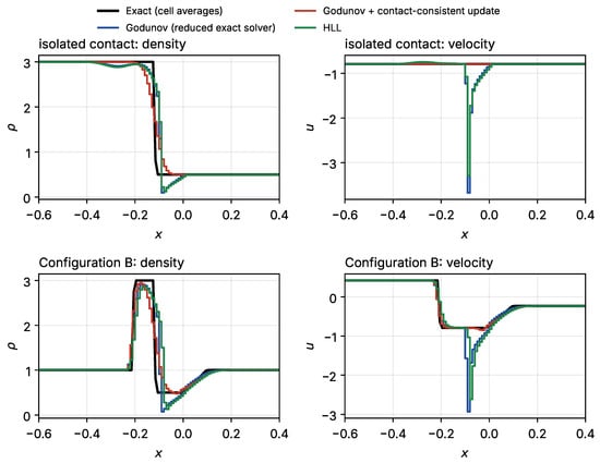
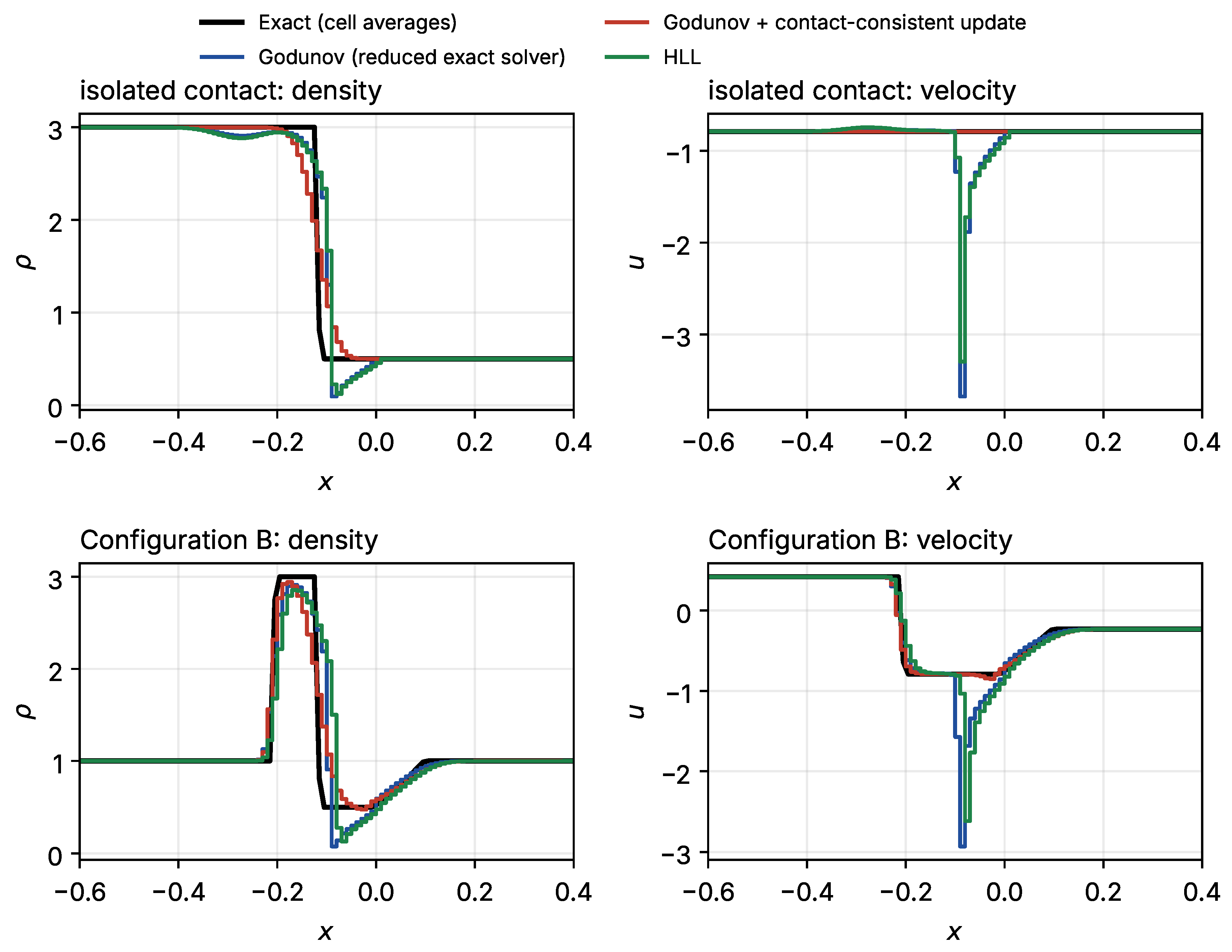
Section 5.3 shows that conservative fluxes produce a velocity spike and a density dip at a contact where q jumps. The exact flux does not cure this. On the isolated contact of Section 5.3 (Table 20), the Godunov, HLL and Rusanov schemes all give velocity errors between 1.3 and 3.1 and density minima between 0.06 and 0.24 (exact minimum 0.5), at every resolution from 100 to 800 cells.

Table 20. Isolated contact ($\rho$: 3.0 → 0.5, $u\equiv -0.7899$, $p+q$ continuous), $t=0.15$: maximum velocity error $\max |u-u^{*}|$ and minimum density (exact: 0 and 0.5).

	Godunov		Godunov + QC		HLL		Rusanov
$\mathit{N}$	$\max |\mathit{u}-{\mathit{u}}^{*}|$	${\mathit{\rho }}_{\min }$	$\max |\mathit{u}-{\mathit{u}}^{*}|$	${\mathit{\rho }}_{\min }$	$\max |\mathit{u}-{\mathit{u}}^{*}|$	${\mathit{\rho }}_{\min }$	$\max |\mathit{u}-{\mathit{u}}^{*}|$	${\mathit{\rho }}_{\min }$
100	2.54	0.096	0.00	0.500	2.07	0.082	1.26	0.237
200	2.89	0.069	0.00	0.500	2.51	0.065	1.83	0.135
400	2.45	0.067	0.00	0.500	3.09	0.064	2.59	0.080
800	1.55	0.067	0.00	0.500	2.17	0.064	2.57	0.071

The defect has a simple cause and a simple remedy. Across a contact, u and $\mathrm{\Pi }=p+q$ are continuous, and for smooth solutions $\mathrm{\Pi }$ obeys

$${\mathrm{\Pi }}_t+u{\mathrm{\Pi }}_x+\rho {\sigma }^2{u}_x=0.$$

(23)

Conservative averaging of $\rho$ and $\rho q$ does not preserve $\mathrm{\Pi }$, because p is nonlinear in $\rho$. We therefore update $\rho$ and $\rho u$ conservatively and, only in cells within two cells of a jump in q, advance $\mathrm{\Pi }$ with an upwind discretisation of (23),

$${\mathrm{\Pi }}_i^{n+1}={\mathrm{\Pi }}_i^n-\frac{\Delta t}{\Delta x}\left[{(u_{i-{\displaystyle \frac{1}{2}}}^{*})}^{+}({\mathrm{\Pi }}_i^n-{\mathrm{\Pi }}_{i-1}^n)+{(u_{i+{\displaystyle \frac{1}{2}}}^{*})}^{-}({\mathrm{\Pi }}_{i+1}^n-{\mathrm{\Pi }}_i^n)+{\rho }_i{\sigma }_i^2(u_{i+{\displaystyle \frac{1}{2}}}^{*}-u_{i-{\displaystyle \frac{1}{2}}}^{*})\right],$$

(24)

with ${\mathrm{\Pi }}^n=p\left({\rho }^n\right)+q^n$, the interface velocities $u^{*}$ of the exact Riemann solutions, and $q^{n+1}={\mathrm{\Pi }}^{n+1}-p\left({\rho }^{n+1}\right)$. This follows the quasi-conservative idea of Abgrall [21]. With u uniform across the contact, (24) advects $\mathrm{\Pi }$ exactly, so the momentum flux sees no spurious gradient.

The contact-consistent update removes the defect on the isolated contact: the velocity stays exact to machine precision and the density never falls below 0.5, at every resolution (Table 20, Figure 11). When the contact separates from a rarefaction (B, C, E), it reduces the velocity error by a factor of 6.7 on B and 4.0 on E, and it raises the minimum density of B from 0.065 to 0.466 (exact 0.5; Table 15). The update has two costs. It gives up exact conservation of $\rho q$: on the configurations with an order-one jump in q, the total of $\rho q$ drifts by 0.03–0.21, against at most 0.004 for the conservative scheme. And when a shock lies within a few cells of the contact (A and Configurations 1 and 3), it increases the density error by a factor of 1.5–6.0, because the non-conservative update then acts across the shock. A switch that applies (24) only where the pressure jump is small would combine the two regimes; we leave its design open.

Figure 11. Isolated contact (top) and Configuration B (bottom) at $N=200$, $t=0.15$: Godunov with and without the contact-consistent update, and HLL.

9. Extension to Two Spatial Dimensions

No two-dimensional version of the Cargo–LeRoux model appears in the published literature. We construct one by advecting q with the full velocity field:

$$U=\left(\begin{array}{c}\rho \\ \rho q\\ \rho u\\ \rho v\end{array}\right),F\left(U\right)=\left(\begin{array}{c}\rho u\\ \rho qu\\ \rho u^2+p+q\\ \rho uv\end{array}\right),G\left(U\right)=\left(\begin{array}{c}\rho v\\ \rho qv\\ \rho uv\\ \rho v^2+p+q\end{array}\right),$$

(25)

which reduces to (1) when $G\equiv 0$. The spectrum in direction x is $u-\sigma ,u,u,u+\sigma$; the middle eigenvalue has multiplicity two, carried by q and v. We discretise (25) with an unsplit first-order Rusanov scheme on uniform Cartesian grids (CFL 0.4, transmissive boundaries).

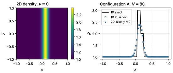
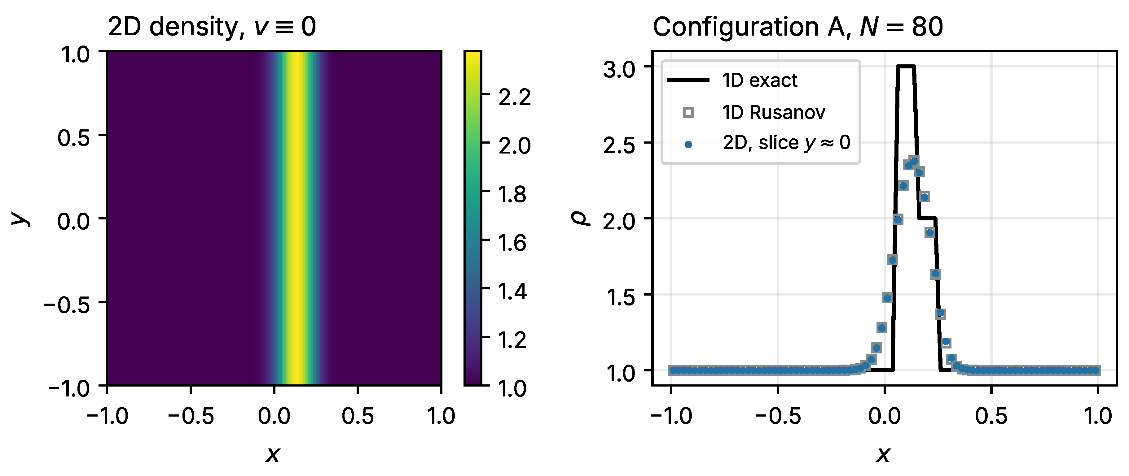
Reduction test. Configuration A with $v\equiv 0$ and x-dependent data must stay independent of y. On an $80\times 80$ grid, the y-variation of the density is exactly zero and v stays exactly zero. The $y=0$ slice differs from the 1D Rusanov solution by at most 0.012 because the 2D time step accounts for both directions (Figure 12).

Figure 12. Reduction test, Configuration A, $N=80$, $t=0.15$. Left: 2D density. Right: the 2D slice at $y\approx 0$ against the 1D Rusanov solution and the exact solution.

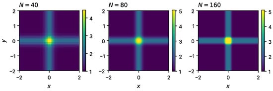
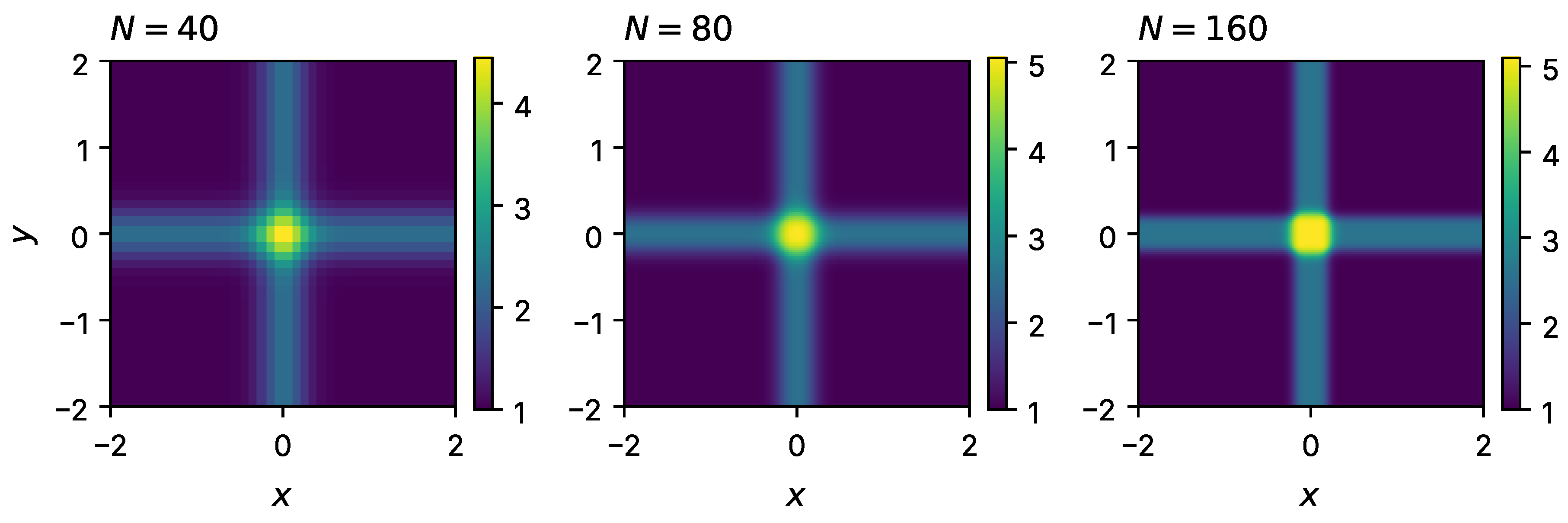
Four-quadrant converging flow. We start from $\rho =1$, $q=0$ and $(u,v)=-U_0(\mathrm{sign}x,$$\mathrm{sign}y)$ on ${[-2,2]}^2$, which compresses the flow onto both axes, and we run to $t=0.3$ at $N=40$–160 for $U_0=1,2,3$. Table 21 shows that the step count grows linearly with N, the density never falls below its initial value 1, $a\rho$ stays at or below 0.544, and the solution keeps its eightfold symmetry to $5\times {10}^{-15}$. A $2\times 2$ odd–even indicator, $\frac{1}{4}|{\rho }_{i,j}-{\rho }_{i+1,j}-{\rho }_{i,j+1}+{\rho }_{i+1,j+1}|$, evaluated for $\left|x\right|,\left|y\right|>0.5$, is at most $9.6\times {10}^{-3}$ at $N=40$, at most $1.0\times {10}^{-5}$ at $N=80$ and at most $3\times {10}^{-10}$ at $N=160$. The scheme shows no corner instability and no checkerboard pattern on these tests (Figure 13).

Table 21. Four-quadrant converging flow, unsplit first-order Rusanov, $t=0.3$. ${\rho }_{\min },{\rho }_{\max }$: extremes over all steps; symmetry: $\max \left(\right|\rho -{\rho }^T|,|\rho -\rho (-x,·)\left|\right)$; odd–even: maximum indicator for $\left|x\right|,\left|y\right|>0.5$ at $t=0.3$.

${\mathit{U}}_0$	N	Steps	${\mathit{\rho }}_{\min }$	${\mathit{\rho }}_{\max }$	$\max \mathit{a}\mathit{\rho }$	Symmetry	Odd–Even
1	40	31	1.000	4.44	0.155	$4\times {10}^{-16}$	$1.4\times {10}^{-3}$
1	80	62	1.000	5.05	0.177	$9\times {10}^{-16}$	$1.0\times {10}^{-5}$
1	120	94	1.000	5.09	0.178	$9\times {10}^{-16}$	$5.4\times {10}^{-8}$
1	160	126	1.000	5.10	0.178	$9\times {10}^{-16}$	$3.0\times {10}^{-10}$
2	40	47	1.000	10.02	0.351	$9\times {10}^{-16}$	$4.3\times {10}^{-3}$
2	80	98	1.000	10.82	0.379	$2\times {10}^{-15}$	$3.1\times {10}^{-6}$
2	120	149	1.000	10.82	0.379	$3\times {10}^{-15}$	$9.3\times {10}^{-10}$
2	160	200	1.000	10.82	0.379	$2\times {10}^{-15}$	$2.5\times {10}^{-13}$
3	40	64	1.000	15.38	0.538	$3\times {10}^{-15}$	$9.6\times {10}^{-3}$
3	80	133	1.000	15.54	0.544	$2\times {10}^{-15}$	$2.0\times {10}^{-6}$
3	120	204	1.000	15.54	0.544	$3\times {10}^{-15}$	$1.7\times {10}^{-10}$
3	160	274	1.000	15.54	0.544	$5\times {10}^{-15}$	$2.0\times {10}^{-14}$

Figure 13. Density of the four-quadrant converging flow, $U_0=1$, $t=0.3$, at $N=40$, 80 and 160.

Arbitrary geometry and irregular boundaries. All tests in this paper use Cartesian grids, and none uses an irregular domain. The three approaches extend to such domains with varied effort.

• NFV needs an unstructured or body-fitted finite-volume mesh. Its flux network would act on face-normal states: one rotates $(u,v)$ into the face frame, applies ${\mathrm{\Phi }}_{\theta }$, rotates back and weights each face flux by its length [3,39]. This relies on the rotational invariance of (25), and it requires training data with all face orientations. Wall faces need a ghost state or a dedicated boundary flux. The cost per step scales with the number of faces, as for a classical scheme. Section 4 also shows that the learned flux is not consistent, so on a new mesh the network would need retraining or a consistency constraint, for instance ${\mathrm{\Phi }}_{\theta }(U_L,U_R)=\frac{1}{2}[F\left(U_L\right)+F\left(U_R\right)]-\frac{1}{2}{D}_{\theta }(U_L,U_R)(U_R-U_L)$ with a learned dissipation $D_{\theta }\ge 0$.
• MoE-PINN extends most naturally because collocation needs no mesh: points are sampled inside the domain and on its boundary, and wall conditions enter the loss. Domain-decomposition variants such as XPINNs [40] assign experts to subdomains, which matches the gated mixture of (14). The training cost scales with the number of collocation points, which must resolve every discontinuity in two space dimensions plus time, and the network must still be retrained for every new initial condition. The smoothing of Section 5 would persist.
• Hybrid exact–NN needs only a one-dimensional Riemann problem normal to each face, so it carries over to unstructured meshes in the same way as a classical Godunov scheme; its cost scales with the number of faces. Its surrogate needs no retraining because it works on face-normal 1D data. With the reduced solver of Section 7, each face solve cannot fail and costs a median of 70 μs, so the cost grows linearly with the number of faces and needs no fallback.

The contact defect of Section 5.3 would carry over to any conservative discretisation on any mesh.

10. Conclusions

This paper gives an exact Riemann solver for the isentropic Cargo–LeRoux model with a closed-form Riemann invariant, and it compares three neural approaches against it. The closed form replaces a tabulated invariant that had overestimated the near-vacuum star density by 64%. The closure is strictly convex; its difficulty lies in the singularity at $a\rho =1$ and in vacuum generation, which system (11) cannot represent.

The star-state system can be posed as constrained residual minimisation, and its constraints decide the outcome. Without entropy constraints, the minimiser of the Rankine–Hugoniot residual contains an expansion shock on 78.6% of well-conditioned cases, and a Godunov scheme built on it forms an expansion shock that does not vanish under refinement. With Lax and rarefaction bounds on each wave configuration, minimisation returns the correct star state on every solvable case and identified every vacuum case. A Godunov scheme driven by it needs no fallback on eleven tests and matches the exact-flux scheme to 8 × 10⁻¹⁰. Eliminating the linearly degenerate contact relation reduces the same problem to a monotone scalar equation whose root exists exactly when no vacuum forms and is then unique. Its bracketed solve has the same reliability at a median of 14 residual evaluations, about $1/116$ of the cost. Newton-type and least-squares solvers on the unconstrained or positivity-bounded residual converge to inadmissible or non-physical points on up to 34.9% of well-conditioned cases. The exact-flux Godunov scheme needs no fallback, stays positive, satisfies the entropy condition at the sonic point, and is the most accurate of three conservative schemes on every test.

MoE-PINN performs like a first-order Rusanov scheme on an 80-cell grid. Its density error grows by a factor of 4.3–8.3 on shock-containing patterns, and substitution into the PDE shows residuals 4–10 times larger near discontinuities than in smooth regions. Its viscosity regularisation lowers the reported residual only near shocks, so a regularised residual understates the PDE violation. NFV conserves exactly but is not consistent with the physical flux. It fits its own training targets 6–34 times more closely than Rusanov, and it loses that advantage on a held-out configuration. A fixed time step did not cause divergence in our implementation, even at a realised CFL number of 5.2.

The admissibility checks show that no method reaches $a\rho \ge 1$, that NFV produces negative densities near vacuum in one of three seeds, and that MoE-PINN collapses to a trivial near-vacuum state in two of three seeds. The NFV velocity overshoots near steep features reach 18%. A classical finding accompanies them: at a contact where q jumps, conservative cell averaging breaks the equilibrium of $p+q$, and both Rusanov and the exact Godunov flux then generate velocity errors above 1.1 and density dips to 0.07–0.28 (exact minimum 0.5) that do not vanish under refinement. Any Godunov-type solver for this model, classical or learned, needs a contact-consistent treatment of q. A quasi-conservative update of $p+q$ near contacts removes the defect exactly on an isolated contact and reduces the velocity error up to 6.7-fold, but it loses exact conservation of $\rho q$ and degrades accuracy when a shock lies next to the contact.

The hybrid scheme’s detector transfers from the HLLC setting and flags every vacuum case of a 400-case stress test, at about 28% extra cost on that mix. Its surrogate, however, returns star states that violate the Riemann relations by 18–25% near vacuum, even where the profile-level error looks small. NFV outperforms MoE-PINN on well-conditioned patterns ($p<0.002$), and no ranking holds near vacuum. A first-order Rusanov discretisation of the two-dimensional extension stays positive, symmetric and free of odd–even patterns up to $N=160$.

Three lessons reach beyond this model. A learned component should be checked at the level of its own output, by substitution into the governing relations, and not only through a downstream error norm. Conservative discretisations of systems in which an advected quantity enters the momentum flux need contact-consistent updates, whether the flux is exact, approximate or learned. And an optimisation-based Riemann solver is only as admissible as its constraint set: the entropy conditions must enter it explicitly, wave by wave.

References

- Lax, P.D. Hyperbolic systems of conservation laws II. Commun. Pure Appl. Math. 1957, 10, 537–566. [Google Scholar] [CrossRef] [Scilit]
- Godunov, S.K. A difference method for numerical calculation of discontinuous solutions of the equations of hydrodynamics. Mat. Sb. 1959, 47, 271–306. [Google Scholar]
- Toro, E.F. Riemann Solvers and Numerical Methods for Fluid Dynamics: A Practical Introduction, 3rd ed.; Springer: Berlin, Germany, 2009. [Google Scholar]
- LeVeque, R.J. Finite Volume Methods for Hyperbolic Problems; Cambridge University Press: Cambridge, UK, 2002. [Google Scholar]
- Raissi, M.; Perdikaris, P.; Karniadakis, G.E. Physics-informed neural networks: A deep learning framework for solving forward and inverse problems involving nonlinear partial differential equations. J. Comput. Phys. 2019, 378, 686–707. [Google Scholar] [CrossRef] [Scilit]
- Karniadakis, G.E.; Kevrekidis, I.G.; Lu, L.; Perdikaris, P.; Wang, S.; Yang, L. Physics-informed machine learning. Nat. Rev. Phys. 2021, 3, 422–440. [Google Scholar] [CrossRef] [Scilit]
- Liu, J.; Zheng, S.; Song, X.; Xu, D. Locally linearized physics-informed neural networks for Riemann problems of hyperbolic conservation laws. Phys. Fluids 2024, 36, 116135. [Google Scholar] [CrossRef] [Scilit]
- Urbán, J.F.; Pons, J.A. An approximate Riemann solver approach in physics-informed neural networks for hyperbolic conservation laws. Phys. Fluids 2025, 37, 096114. [Google Scholar] [CrossRef] [Scilit]
- Ruggeri, M.; Roy, I.; Mueterthies, M.J.; Gruenwald, T.; Scalo, C. Neural-network-based Riemann solver for real fluids and high explosives; application to computational fluid dynamics. Phys. Fluids 2022, 34, 116121. [Google Scholar] [CrossRef] [Scilit]
- Cargo, P.; LeRoux, A.Y. Un schéma équilibre adapté au modèle d’atmosphère avec termes de gravité. C. R. Acad. Sci. Paris 1994, 318, 73–76. [Google Scholar]
- Jana, S.; Kuila, S. Exact solution of the flux perturbed Riemann problem for Cargo–LeRoux model in a van der Waals gas. Chaos Solitons Fractals 2022, 161, 112369. [Google Scholar] [CrossRef] [Scilit]
- Karna, A.K.; Satapathy, P. Lie symmetry analysis for the Cargo–LeRoux model with isentropic perturbation pressure equation of state. Chaos Solitons Fractals 2023, 177, 114241. [Google Scholar] [CrossRef] [Scilit]
- Sahoo, S.M.; Sekhar, T.R.; Raja Sekhar, G.P. Wave interactions in pressureless Cargo–LeRoux model with flux perturbation. Math. Methods Appl. Sci. 2023, 46, 8663–8679. [Google Scholar] [CrossRef] [Scilit]
- Khan, I.; Ahmed, S.; Rauf, A.; Koh, W.S. Numerical solution to the Cargo LeRoux model. Contemp. Math. 2026, 7, 1055–1067. [Google Scholar] [CrossRef] [Scilit]
- Lichtlé, N.; Canesse, Q.; Fu, Z.; Matin, N.; Delle Monache, M.L.; Bayen, A. (U)NFV: Supervised and unsupervised neural finite volume methods for solving hyperbolic PDEs. arXiv 2025, arXiv:2505.23702. [Google Scholar]
- Bischof, R.; Kraus, M.A. Mixture-of-experts-ensemble meta-learning for physics-informed neural networks. In Proceedings of the 33rd Forum Bauinformatik, Munich, Germany, 7–9 September 2022. [Google Scholar]
- Dan, J.; Sun, J.; Li, J.; Shi, S. An adaptive optimal selection approach of the mixture-of-experts model embedded with PINNs for one-dimensional hyperbolic conservation laws. Commun. Nonlinear Sci. Numer. Simul. 2025, 149, 108936. [Google Scholar] [CrossRef] [Scilit]
- Fuks, O.; Tchelepi, H.A. Limitations of physics informed machine learning for nonlinear two-phase transport in porous media. J. Mach. Learn. Model. Comput. 2020, 1, 19–37. [Google Scholar] [CrossRef] [Scilit]
- Lax, P.D.; Wendroff, B. Systems of conservation laws. Commun. Pure Appl. Math. 1960, 13, 217–237. [Google Scholar] [CrossRef] [Scilit]
- Nogueira, X.; Ramos, L.; Seijo, S.; Couceiro, I.; Khelladi, S.; Ramírez, L. Data-driven Riemann solvers: A neural network approach and a hybrid solver. Phys. Fluids 2025, 37, 096142. [Google Scholar] [CrossRef] [Scilit]
- Abgrall, R. How to prevent pressure oscillations in multicomponent flow calculations: A quasi conservative approach. J. Comput. Phys. 1996, 125, 150–160. [Google Scholar] [CrossRef] [Scilit]
- Majda, A.; Osher, S. Numerical viscosity and the entropy condition. Commun. Pure Appl. Math. 1979, 32, 797–838. [Google Scholar] [CrossRef] [Scilit]
- Kružkov, S.N. First order quasilinear equations in several independent variables. Math. USSR-Sb. 1970, 10, 217–243. [Google Scholar] [CrossRef] [Scilit]
- Rusanov, V.V. The calculation of the interaction of non-stationary shock waves and obstacles. USSR Comput. Math. Math. Phys. 1962, 1, 304–320. [Google Scholar] [CrossRef] [Scilit]
- Perthame, B.; Shu, C.-W. On positivity preserving finite volume schemes for Euler equations. Numer. Math. 1996, 73, 119–130. [Google Scholar] [CrossRef] [Scilit]
- Zhang, X.; Shu, C.-W. On positivity-preserving high order discontinuous Galerkin schemes for compressible Euler equations on rectangular meshes. J. Comput. Phys. 2010, 229, 8918–8934. [Google Scholar] [CrossRef] [Scilit]
- Toro, E.F.; Spruce, M.; Speares, W. Restoration of the contact surface in the HLL-Riemann solver. Shock Waves 1994, 4, 25–34. [Google Scholar] [CrossRef] [Scilit]
- Smoller, J. Shock Waves and Reaction–Diffusion Equations, 2nd ed.; Springer: New York, NY, USA, 1994. [Google Scholar]
- Godlewski, E.; Raviart, P.-A. Numerical Approximation of Hyperbolic Systems of Conservation Laws; Springer: New York, NY, USA, 1996. [Google Scholar]
- Branch, M.A.; Coleman, T.F.; Li, Y. A subspace, interior, and conjugate gradient method for large-scale bound-constrained minimization problems. SIAM J. Sci. Comput. 1999, 21, 1–23. [Google Scholar] [CrossRef] [Scilit]
- Brent, R.P. Algorithms for Minimization Without Derivatives; Prentice-Hall: Englewood Cliffs, NJ, USA, 1973. [Google Scholar]
- Moré, J.J.; Garbow, B.S.; Hillstrom, K.E. User Guide for MINPACK-1; Report ANL-80-74; Argonne National Laboratory: Argonne, IL, USA, 1980. [Google Scholar]
- Broyden, C.G. A class of methods for solving nonlinear simultaneous equations. Math. Comp. 1965, 19, 577–593. [Google Scholar] [CrossRef]
- Levenberg, K. A method for the solution of certain non-linear problems in least squares. Quart. Appl. Math. 1944, 2, 164–168. [Google Scholar] [CrossRef] [Scilit]
- Marquardt, D.W. An algorithm for least-squares estimation of nonlinear parameters. J. Soc. Ind. Appl. Math. 1963, 11, 431–441. [Google Scholar] [CrossRef] [Scilit]
- Harten, A.; Lax, P.D.; van Leer, B. On upstream differencing and Godunov-type schemes for hyperbolic conservation laws. SIAM Rev. 1983, 25, 35–61. [Google Scholar] [CrossRef] [Scilit]
- Davis, S.F. Simplified second-order Godunov-type methods. SIAM J. Sci. Stat. Comput. 1988, 9, 445–473. [Google Scholar] [CrossRef] [Scilit]
- Colella, P. Glimm’s method for gas dynamics. SIAM J. Sci. Stat. Comput. 1982, 3, 76–110. [Google Scholar] [CrossRef] [Scilit]
- Barth, T.J.; Jespersen, D.C. The design and application of upwind schemes on unstructured meshes. In Proceedings of the 27th Aerospace Sciences Meeting, Reno, NV, USA, 9–12 January 1989. [Google Scholar]
- Jagtap, A.D.; Karniadakis, G.E. Extended physics-informed neural networks (XPINNs): A generalized space–time domain decomposition based deep learning framework for nonlinear partial differential equations. Commun. Comput. Phys. 2020, 28, 2002–2041. [Google Scholar] [CrossRef] [Scilit]
Disclaimer/Publisher’s Note: The statements, opinions and data contained in all publications are solely those of the individual author(s) and contributor(s) and not of MDPI and/or the editor(s). MDPI and/or the editor(s) disclaim responsibility for any injury to people or property resulting from any ideas, methods, instructions or products referred to in the content. |
© 2026 by the authors. Licensee MDPI, Basel, Switzerland. This article is an open access article distributed under the terms and conditions of the Creative Commons Attribution (CC BY) license.