


Abstract
Meritocratic lotteries seek to implement prescribed selection probabilities reflecting merit or priority while meeting diversity quotas. We study this implementation problem on a hypergraph, with arbitrary target marginals and integer lower and upper quotas. Assuming consistency of the target marginals with the quotas and prescribed group size, we adapt existing decomposition and rounding results to establish two guarantees: (1) exact quota compliance when the traits admit a partition into two disjoint-set families; and (2) for general trait hypergraphs, a violation of each quota by at most , where D is the maximum number of traits possessed by an agent. Both constructions preserve all marginals and the group size exactly, run in polynomial time, and produce explicit lotteries supported on at most as many selected groups as there are agents. The explicit lists of groups and their probabilities allow organisers to publish and inspect these lotteries before the draw. We then obtain trait-specific bounds when a small set of agents has high trait overlap and a concentration-based guarantee allowing small marginal errors. Applications to representative selection illustrate the trade-off between exact marginal implementation and exact quota compliance.
Keywords:
randomized rounding; discrepancy theory; hypergraphs; convex decomposition; overlapping quotas; committee selection; random allocation MSC:
05C65; 90C27
1. Introduction
Selection procedures often seek to reconcile meritocracy with diversity. An institution may wish to honor individual selection probabilities reflecting merit or priority while ensuring representation across overlapping traits. Lotteries provide a way to implement these probabilities when selecting a group of a prescribed size. Representation requirements arise in citizens’ assemblies, admissions lotteries, juries, and the allocation of public-program places [1,2,3]. The resulting mathematical question is whether a prescribed vector of selection probabilities can be expressed as a lottery over groups that satisfy every representation quota.
Let be a finite population, let be a family of nonempty traits, and fix a target vector with . Each trait has integer lower and upper quotas and . We seek a distribution over sets with such that
in every outcome. A necessary condition is consistency: for every trait. Overlap between traits can prevent this expectation-level condition from being sufficient.
The target probabilities may reflect merit, priorities, needs, or entitlements, or may be uniform. Weighted admissions and medical-allocation lotteries provide examples [4,5,6]. When the targets encode merit or priority, we interpret their exact implementation as meritocracy and call the resulting lottery meritocratic. We take the targets as given and do not prescribe how merit or priority should be assessed. In the formal definitions and results, we use marginal preservation for exact implementation of the target probabilities, because the results apply to any consistent target vector. Representation requirements can refer to several attributes and their intersections, so the traits need not form partitions or nested families.
Two parameters of the trait hypergraph play distinct roles. Its chromatic index is the minimum number of families of pairwise disjoint traits into which can be partitioned; we call these families dimensions. Its maximum degree is the largest number of quotas affected by one selection. Always , but their ratio can be arbitrarily small. This distinction separates the structure needed for exact implementation from the sparsity governing additive approximation.
We first give a constructive exact benchmark for (Theorem 1). Consistency then suffices. The existence result follows from standard network integrality and is a special case of the bihierarchy framework of Budish et al. [1]. We provide a direct circulation construction, a mean-preserving cycle-rounding implementation, and an explicit lottery supported on at most groups. Examples with three dimensions show that this sufficient condition cannot be extended to all higher-dimensional instances.
For arbitrary trait hypergraphs, Theorem 2 constructs a lottery that preserves all marginals and the group size exactly and violates every quota by at most . The rounding step adapts the algorithm of Flanigan et al. [7] to the present trait-hypergraph setting. The algorithm combines Beck–Fiala floating-variable rounding [8] with repeated support reduction. It belongs to the sparse approximate-decomposition tradition of Nguyen et al. [9]. Our formulation accommodates arbitrary overlapping traits and consistent two-sided quotas, and its deterministic output is an explicit distribution over at most groups. The bound depends on the number of constraints involving an individual, rather than on the number of trait dimensions.
The explicit representation of the lottery has practical value, particularly for sortition. The algorithm produces a list of at most selected groups together with their probabilities. Organisers can publish or print this list before conducting the draw. Each group’s size and quota compliance, up to the stated approximation guarantee, can be checked directly. Likewise, each individual’s prescribed selection probability can be verified by summing the probabilities of the listed groups containing that individual. The final selection then requires only a draw from this explicitly specified finite lottery. Thus, the support reduction makes the construction transparent and readily inspectable, in addition to keeping its representation small.
We develop two complementary refinements. First, if most agents have low degree, the guarantee need not be determined by the few agents who have many traits. For an exceptional set , Theorem 3 bounds the violation of trait e by , where is the largest degree outside B. Thus, at most r agents with degree above d yield a uniform bound of . Second, Theorem 4 combines dependent rounding [10] with rejection sampling. Allowing marginal errors of at most gives a quota bound of order , which can be useful when the maximum degree is large.
The results yield a design alternative to procedures that impose exact quotas and optimize the resulting marginal probabilities. In particular, LEXIMIN [2] prioritizes exact representation and then makes selection probabilities as equal as possible. Our construction preserves an externally specified vector and makes the required quota relaxation explicit. A small example shows that even when exactly diverse groups exist, preserving uniform marginals can require relaxing a quota. An illustration using citizens’ assembly data reports substantially smaller quota deviations than the worst-case bound. We also discuss type compression and the limited incentive implication of maintaining marginals independently of reported traits.
Section 2 positions the results in the related literature. Section 3 presents the model and its matrix formulation. Section 4 and Section 5 give the exact and approximate implementation results. Section 6 discusses implementation and applications, and Section 7 concludes. Detailed proofs appear in Appendix A.
2. Related Literature
Apportionment and panel-selection rounding. Cembrano et al. [11] study multidimensional political apportionment (other related papers in apportionment include [12,13,14]). Like us, they identify a sharp two-versus-three-dimensional divide: exact proportionality is guaranteed in two dimensions but may fail with three or more, and they provide approximation guarantees for higher dimensions. Our results differ from theirs in three respects. First, our object is a lottery over selected groups with prescribed individual marginals, rather than an apportionment vector. Second, our model incorporates arbitrary ex ante target probabilities p in addition to ex post representation quotas. Third, our approximation guarantee depends on , the maximum number of traits possessed by an agent, rather than on the number of dimensions. Since the former is weakly smaller than the latter, and the gap can be arbitrarily large, this distinction can be substantial.
Flanigan et al. [7] [Lemmas 3 and 9] present a result closely related to Theorem 2. Conditional on a realized volunteer pool, they start from individual marginals summing to the panel size and use Beck–Fiala floating-variable rounding [8] to preserve these marginals and the panel size, while keeping each trait count within an additive error equal to the exogenously specified number of dimensions minus one (although their displayed guarantee uses a weak bound equal to the number of dimensions, their proof yields a strict error smaller than that number; consequently, when expressed relative to consistent integer quotas, their argument gives the same one-unit refinement as Theorem 2 in their feature-partition setting). In their model, every agent possesses exactly one trait in each dimension. By contrast, Theorem 2 applies to arbitrary trait hypergraphs in which agents need not possess a trait in every dimension, accommodates arbitrary consistent lower and upper quotas, and produces in polynomial time an explicit lottery with support size at most . Their polynomial-time result instead provides a sampling procedure; their alternative column-generation method constructs an explicit distribution but is not guaranteed to run in polynomial time. Finally, our degree-based formulation can yield a substantially smaller bound when the maximum number of traits possessed by an agent is strictly smaller than the number of dimensions.
Sparse approximate decomposition. Nguyen et al. [9] [Theorem 2.1] show that a fractional assignment of bundles can be implemented as a lottery over integral assignments, preserving the fractional assignment exactly and over-allocating each good by at most the maximum bundle size minus one. Viewing an agent’s traits as a bundle connects that size parameter to the column sparsity of our trait-incidence matrix. Their result therefore already establishes the combination of exact marginal preservation and a sparsity-minus-one additive relaxation. The direct candidate-as-bundle interpretation does not itself impose a fixed number of selected candidates in every realization. We give a direct construction for fixed-size subsets with overlapping lower and upper quotas, together with the exceptional-agent and approximate-marginal refinements below. The degree-based bound should thus be understood within this established sparse-rounding framework.
Network flows, b-matchings, and dependent rounding. After adding trivial traits where needed, the two-dimensional case can be viewed as a bipartite b-matching problem with lower and upper degree bounds and fixed cardinality: traits form the two vertex classes, and agents correspond to unit-capacity edges. Theorem 1 gives a direct lottery implementation of the associated integral-flow formulation [15]. For Theorems 1 and 2, Appendix A.2 combines mean-preserving rounding with Carathéodory support reduction to construct explicit lotteries over fixed-size subsets. Theorem 4 instead applies the dependent-rounding and concentration results of Gandhi et al. [10], followed by rejection sampling, to obtain simultaneous quota guarantees with small marginal errors.
Diverse committees, sortition, and citizens’ assemblies. A growing literature studies representative committees and citizens’ assemblies, including diverse representation, multiwinner selection with diversity constraints, and sortition [16,17,18,19,20,21,22,23,24,25]. Another important benchmark is the LEXIMIN approach of Flanigan et al. [2], which restricts attention to exactly quota-feasible panels and then makes individual selection probabilities as equal as possible. We compare our algorithm with LEXIMIN in Section 6.
Random allocation, priorities, and implementable lotteries. A central question in random allocation is when a desired fractional assignment can be implemented as a lottery over deterministic feasible outcomes. In classical random assignment, the Birkhoff–von Neumann decomposition underlies lottery implementations of doubly stochastic matrices and mechanisms such as probabilistic serial [26,27]. Budish et al. [1] extend this logic to random allocation with additional constraints, identifying structural conditions, such as bi-hierarchical constraints, that allow fractional allocations to be decomposed into feasible deterministic outcomes. Indeed, the existence part of Theorem 1 can be viewed as a special case of their bihierarchy result: when traits can be partitioned into two dimensions, the two families of pairwise-disjoint traits form two hierarchies, so consistency implies that the target marginal vector can be decomposed into quota-feasible selected groups. More recent work studies priorities, constraints, and approximate implementability in random allocation [28,29,30,31].
Our question belongs to this implementability tradition, but with differently structured constraints. Trait quotas are overlapping and intersectional: a selected agent may affect many constraints, and the traits need not be disjoint or nested. We take an arbitrary target marginal vector p and ask whether it can be decomposed into a lottery over groups satisfying, or approximately satisfying, every quota ex post.
Distributional constraints in market design. Distributional constraints are central in market design, especially in school choice, affirmative action, and matching with regional or type-specific quotas. The school-choice framework of Abdulkadiroğlu and Sönmez [3] and subsequent work on controlled choice and affirmative action study how priorities, preferences, and constraints interact [32,33]. Kamada and Kojima [34,35,36] analyze matching with distributional constraints, including existence, stability, efficiency, and strategy-proofness issues. Carvalho et al. [37] emphasize that single-dimension affirmative-action policies can miss important intersectional effects.
Relative to this literature, our model abstracts from preferences and strategic behavior. In applications such as sortition, juries, and lotteries among qualified applicants, the central institutional question is often not which object an agent prefers, but whether a prescribed priority vector can be implemented without violating representation constraints. Our results characterize this implementation problem under intersectional quotas.
3. Model
Setting. We study the problem of selecting a group of k agents from a finite population, subject to target ex ante selection probabilities and ex post diversity requirements. Depending on the context, the selected group may represent a committee, a citizens’ assembly, a jury, a scholarship cohort, or an admissions class.
Formally, a setting is a tuple , where:
- 1.
- is a finite nonempty set of agents.
- 2.
- is a finite nonempty set of nonempty subsets of agents.
- 3.
- is the target selection probability of each agent v, where .
- 4.
- is the lower bound on the number of selected agents with each trait e.
- 5.
- is the upper bound on the number of selected agents with each trait e.
- 6.
- is the number of selected agents.
We interpret each as a diversity trait. For every and , membership indicates that agent v has trait e, and indicates that agent v does not have trait e. Observe that constitutes a finite hypergraph (a hypergraph is a pair of a vertex set and a collection of subsets of , called hyperedges).
Quota Feasibility and Marginal Preservation. We require the random selection process to satisfy:
- 1.
- ex post diversity: The number of selected agents with each trait e must be between and .
- 2.
- ex ante marginal preservation: Each agent v should be selected with probability . The target vector may represent merit, need, entitlement, or equal treatment; its interpretation is separate from the implementation problem.
A selected group (of size k) is a subset of k agents, i.e., a set satisfying . A selected group S is diverse if the number of selected agents with each trait is between the trait’s lower bound and its upper bound, i.e., if for each trait .
Denote the set of all selected groups of size k by . A k-selection lottery is a distribution over selected groups of size k. Given a k-selection lottery and an agent v, let be the marginal selection probability of agent v. We say that a k-selection lottery is marginal-preserving if for each agent v, and we say that it is diverse if every selected group in its support is diverse.
Matrix formulation and computational conventions. Let , and define the incidence matrix by if and only if . Write for the incidence vector of S. The problem is to find weights and sets such that
Consistency means . The parameter is the maximum column sum of A, whereas two-dimensionality is a structural restriction on its rows. An explicit lottery consists of the sets and their probabilities . Throughout, input probabilities are rational and encoded in binary, quotas are integers, and polynomial time refers to the total encoding length, including the trait-incidence data. Bounds stated in terms of numbers of agents and traits use this convention.
Remark 1.
The target selection probabilities may themselves be derived from a social-welfare objective. For example, suppose that society evaluates a k-selection lottery μ according to , where represents the merit or priority weight assigned to agent v. Maximizing W over all k-selection lotteries is equivalent to maximizing it over all marginal vectors satisfying . Provided that for every the unique welfare-maximizing marginal probabilities are for every Thus, the target probabilities may be interpreted as the welfare-maximizing probabilities associated with society’s merit or priority weights.
Dimensionality. It turns out that the ability to achieve both marginal preservation and diversity crucially depends on the dimensionality of the traits, which is the minimum number of classes (dimensions) into which the set of traits can be partitioned, such that all traits within the same dimension are pairwise disjoint. For example, the different dimensions might be race, gender, socioeconomic status, and locale type.
Formally, the dimensions correspond to a proper edge-coloring of the hypergraph : each color class represents one dimension, and the hyperedges of that color represent the traits within that dimension (e.g., for gender, or for locale type). Properness means that hyperedges (traits) of the same color are pairwise disjoint. Thus, the chromatic index , i.e., the minimum number of colors in a proper edge-coloring of the hypergraph, captures the dimensionality of the traits. Henceforth, we define the number of dimensions in a setting as the chromatic index .
Examples
Real-world examples. Various random selection processes require ex ante marginal preservation, ex post diversity, or both. The simplest case is the equal-priority case, in which all agents are entitled to the same ex ante probability of selection. This arises, for example, in some forms of jury selection, citizens’ assemblies, and school admission lotteries, where uniform randomization is used to treat similarly situated candidates symmetrically.
In other settings, the required selection probabilities are non-uniform and reflect heterogeneity in merit, priority, need, or entitlement. Some examples include:
- GPA-band weighted lottery. For several decades, admission to Dutch medical schools was based on a national weighted lottery. Applicants with higher GPAs received higher lottery weights, with students in the highest GPA category having about three times the selection probability of those in the lowest category [4].
- Charter-school weighted admissions lottery. Some charter schools use weighted admissions lotteries, giving priority applicants higher selection probabilities [5]. For example, a Jersey City charter school doubles the lottery weight of applicants receiving certain forms of public assistance [38].
- Weighted lottery for scarce medical treatments. During COVID-19 shortages, some health systems allocated scarce therapeutics by weighted lottery, giving higher chances to patients with ethical or medical priority factors, such as essential-worker status, social disadvantage, or expected clinical benefit [6].
Various selection procedures include ex post diversity quotas. Some examples include:
- Citizens’ assemblies. Random selection processes for citizens’ assemblies typically try to implement either approximately equal or non-uniform selection probabilities that compensate for non-uniform response rates [7], subject to the constraint that the resulting assembly satisfies diversity quotas across dimensions. For example, the Irish Citizens’ Assembly was required to satisfy diversity quotas in four dimensions: gender, age, region, and social class [39].
- Affordable housing. Affordable housing is often allocated by lottery under the constraint that the share of units allocated to applicants with disabilities must meet a specified minimum quota; for example, 7% in NYC [40].
- Diversity quotas for juries. Several Argentine provinces require a 12-person criminal jury to be composed of six women and six men. In addition, when an Indigenous defendant faces a criminal jury trial in Chaco province, at least 6 of the jurors must belong to the defendant’s Indigenous community [41].
Illustrative examples. We illustrate our model with two simple examples.
Example 1.
Consider 6 agents and 3 diversity dimensions: locale type, age, and height. Each agent has exactly two traits (and has no diversity trait in the remaining dimension): Agent 1 is urban and old; Agent 2 is old and tall; Agent 3 is rural and short; Agent 4 is urban and tall; Agent 5 is young and short; and Agent 6 is rural and young. Thus, each trait is held by exactly two agents. This is represented by , and The hypergraph is 2-uniform, hence a graph, and consists of two disjoint triangles; its chromatic index is 3. The left panel of Figure 1 depicts with a proper 3-edge-coloring, where colors correspond to dimensions.
Figure 1.
Trait hypergraphs. The (left) panel shows the two disjoint triangles of Example 1 with a proper 3-edge-coloring. The (right) panel shows the hypergraph of Example 2 with a proper 2-edge-coloring.
Let , and require each trait to be represented by at least one selected agent, i.e., and for every . The group is not diverse, since it contains no young agents. In contrast, is diverse, since every trait has a selected member. Assume that we require equal selection probability for all agents, i.e., for each . Consider the set consisting of selected groups with two members from and two members from , i.e., Clearly, every selected group in is diverse. Let μ be the uniform distribution over . Observe that μ is marginal-preserving (i.e., for each ) and diverse.
Example 2.
Consider a population of six agents with two diversity dimensions—age and height—where each dimension has two traits. Agents 1 and 2 are old and tall; Agent 3 is old and short; Agent 4 is young and tall; Agent 5 is young and has no height trait; and Agent 6 is young and short. The right panel of Figure 1 illustrates the resulting hypergraph. Observe that the chromatic index of the hypergraph is 2.
4. Results with Exact Diversity
4.1. Consistent Settings
A setting is consistent if for each trait e, and it is inconsistent otherwise. Observe that when the setting is inconsistent, every selection lottery must violate either diversity or marginal preservation.
Claim 1.
If a setting is inconsistent, then any lottery over selected groups must violate either diversity or marginal preservation.
Proof.
Since the setting is inconsistent, there is a trait such that . Suppose, toward a contradiction, that a lottery satisfies both marginal preservation and diversity. By marginal preservation, for every , so the expected number of selected agents with trait e is . Since satisfies diversity, every selected group S in its support satisfies , and hence . This contradicts . □
Thus, in what follows, we focus on conditions for the existence of diverse and marginal-preserving selection processes in consistent settings.
4.2. Exact Diversity with Two Dimensions
In this section, we restrict attention to settings with at most two diversity dimensions (e.g., race and gender), i.e., . It is well known that one can decide in polynomial time whether a hypergraph has chromatic index at most 2 (however, determining the exact value of is NP-hard in general). Thus, one can decide in polynomial time whether a setting admits a representation using at most two dimensions. For completeness, we include a proof in Appendix A.1.
Fact 1.
There exists an algorithm that, given a hypergraph , runs in time polynomial in and decides whether .
The following constructive form of the network-integrality benchmark shows that when there are at most two dimensions (i.e., ), diverse and marginal-preserving k-selection lotteries always exist. Moreover, they can be found with running time polynomial in the number of agents () and traits ().
Theorem 1.
There exists an algorithm that, given a consistent setting with , runs in time polynomial in and outputs an explicit description of a diverse and marginal-preserving k-selection lottery μ with support size at most .
The formal proof of Theorem 1 appears in Appendix A.3. It combines an auxiliary circulation-graph construction in the spirit of [42] with a rounding scheme in the spirit of [10]. We now sketch the proof outline.
Let be a partition of the hyperedges into two color classes (the two trait dimensions). Without loss of generality, assume ; otherwise, for each such that , add to an auxiliary hyperedge that includes the agents with no trait in dimension i. We assign this auxiliary hyperedge trivial bounds 0 and k, so it imposes no additional diversity constraint. Any solution for the augmented hypergraph (with the added auxiliary hyperedge) is also a solution for the original. We treat traits in the two color classes as distinct labeled copies, even if two augmented subsets coincide. Since hyperedges of the same color form a partition of , each vertex belongs to exactly one hyperedge of and one hyperedge of .
We now construct an auxiliary directed multigraph (a directed multigraph allows multiple directed edges between the same ordered pair of vertices). (following [42]) in which: (1) the set of vertices is the hyperedges of (with the added auxiliary hyperedges mentioned above) and two distinguished vertices s and t arranged in four tiers, and (2) the arc set consists of one arc for each , one arc for each agent , one arc for each , and one arc . The arcs from s to and from to t correspond to traits (elements of ) and the arcs from to correspond to agents (elements of ). The edges are described in Table 1 and illustrated for the setting of Example 2 in Figure 2.
Table 1.
Arcs and flows in the auxiliary circulation graph G.
Figure 2.
Auxiliary circulation graph for Example 2, with , , , and .
For each vertex , let and denote the set of outgoing and incoming edges of v, respectively. A circulation is a vector that assigns a real value to each edge of G while satisfying flow conservation, i.e., for every vertex, the inflow equals the outflow:
Table 1 specifies an initial circulation , which represents the target marginal selection probabilities . Observe that this initial circulation satisfies flow conservation.
Starting from , we repeatedly apply a standard cycle-based perturbation argument (see, e.g., [15] [Section 9.6]), which gradually turns fractional arc flows into the neighboring integers while preserving flow conservation. At each step, let denote the current circulation, and consider an undirected multigraph F obtained from G by removing the arcs whose current flow is integral. If this multigraph were acyclic, it would have a leaf vertex v. Then exactly one edge incident to v would be fractional, while all others would be integral, which contradicts flow conservation at v. Hence F contains an undirected cycle C, possibly of length two. Fix such a cycle C and choose an arbitrary traversal direction. Define a signed circulation that assigns to each arc of C whose orientation agrees with the chosen traversal direction and to each arc whose orientation disagrees with it, and 0 to all other edges (not in C).
Observe that satisfies flow conservation. Let be maximal such that and remain within the current floor–ceiling bounds, i.e., for every . By maximality, at least one additional edge becomes integral in each of . We randomize between them so that the expected flow remains , choosing with probability . Thus the expected final circulation remains . Each step strictly reduces the number of fractional edges, so after at most steps we obtain an integer circulation. This circulation corresponds to a diverse selected group; since its expectation is , the induced lottery is marginal-preserving. Finally, by Carathéodory’s theorem, because all diverse selected-group incidence vectors lie in the affine hyperplane of dimension at most , the marginal vector p can be expressed as a convex combination of at most diverse selected groups. Hence the lottery has support size at most .
Figure 2 illustrates the auxiliary multigraph for the setting of Example 2 with selected group size , uniform selection probabilities , and diversity quotas and for each trait e. The figure shows the initial flow , an undirected cycle C (the diamond-like shape marked with thick yellow lines), one possible flow after a single cycle-perturbation step with respect to C, and one possible realization for the final integer flow. The final integer flow corresponds to a diverse committee that includes agent 1 (old and tall), agent 3 (old and short) and agent 5 (young with no height trait).
4.3. Impossibility in High Dimensions ()
The following example illustrates that even a small deviation from the two-dimensional case is sufficient to make diverse selected groups infeasible. Specifically, we revisit Example 1, where there are three dimensions and each agent has two diversity traits, and we show that no diverse selected groups of size 3 exist.
Example 1 (cont.).
We change the selected group size to be and the uniform selection probability to be . Suppose, for contradiction, that there exists a diverse selected group of size 3. Observe that the selected group has at most one member from one of the “triangles” in the left panel of Figure 1, i.e., either or . The former (resp., latter) implies that the selected group misses at least one of the following traits: urban, old, or tall (resp., rural, young, or short). This contradicts S being diverse because there is a trait e with no selected members even though .
In Example 1, any selected group falls short of diversity by at most one member for each trait (i.e., for some traits it has 0 members where the lower quota is 1). By contrast, the next example shows that for any n, there exists a consistent setting in which every selected group falls short by at least n members for some trait.
Example 3.
Let be a setting with and , where the hyperedges are all -element subsets of . Assume uniform selection probabilities, for each , and require each trait to have at least n selected members, i.e., and for every . The setting is consistent. However, any selected group of size contains no members of its complement , which is itself a -element trait. Since this trait has lower quota n, the group S falls short by n members.
5. Approximate Diversity
5.1. Few Diversity Traits per Agent
In many applications, the maximum number of diversity traits held by a single agent is small (e.g., four in the Irish citizens’ assembly application [39] and at most eight and typically fewer in the applications analyzed in [2]). Our next result (Theorem 2) shows an efficient algorithm to construct a marginal-preserving k-selection lottery that is approximately diverse. The approximation error is additive and strictly smaller than the maximum number of traits held by any single agent.
We say that a selected group is d-approximately diverse if no diversity trait is either underrepresented or overrepresented in the selected group by more than d members. Formally,
Definition 1.
Fix a setting and . A selected group is d-approximately diverse if for every , . A k-selection lottery is d-approximately diverse if all selected groups in its support are d-approximately diverse.
The number of diversity traits of agent v is captured by its degree in the hypergraph . The maximum degree of the hypergraph, , captures the intersectionality of the traits, i.e., the maximum number of traits held by a single agent.
Our next result shows that any consistent setting admits a marginal-preserving and -approximately diverse selection lottery. Moreover, such a selection lottery can be implemented in polynomial time. Note that the maximum degree of is always at most the number of dimensions (i.e., ), and the gap between them can be arbitrarily large (for any , let and let , where . Then every vertex lies in exactly two hyperedges ( and ), so . Moreover, any two hyperedges intersect in , and therefore there are m dimensions ()). Note that the related approximation notions in [7,11] scale with the number of dimensions, making it uninformative when agents have far fewer traits than there are dimensions, i.e., .
Example 1 shows that the guarantee is tight when : exact diversity may be impossible, whereas Theorem 2 guarantees 1-approximate diversity. Our analysis leaves open whether the bound is tight for higher values of .
Theorem 2.
There exists an algorithm that, given a consistent setting , runs in time polynomial in and outputs a marginal-preserving and -approximately diverse k-selection lottery with support size at most .
The sparsity-minus-one form of this guarantee is closely related to the approximate decomposition of Nguyen et al. [9] and to the algorithm of Flanigan et al. [7]; see Section 2. The construction below keeps the cardinality equation exact throughout the rounding process.
The formal proof is presented in Appendix A.4. Its main steps also give a sampling implementation. Let . Start from , and at each stage let
Keep integral coordinates fixed, preserve , and preserve the trait sums for all . These requirements admit a nonzero perturbation direction whenever is nonintegral. To see the key point, set and identify repeated restrictions . If there are r distinct large restrictions, incidence counting gives . Including the cardinality equation still leaves fewer than m independent equations: if , then , so any large restriction must be the whole fractional set and the cardinality equation is redundant. If there are no large restrictions, integrality of k excludes . Lemma A2 gives the full argument.
Choose a nonzero direction satisfying these homogeneous equations and move to the two endpoints of the feasible line segment in . Each endpoint has at least one additional integral coordinate. Randomizing between the endpoints to preserve the current vector in expectation preserves every target marginal. The cardinality equation is maintained deterministically at every step.
For a fixed trait e, its sum remains equal to until at most D of its coordinates are fractional. Each remaining coordinate can subsequently change by less than one, giving
Consistency and the integrality of the quotas then yield
Thus the process terminates after at most steps along each sampled path. To produce an explicit lottery without expanding the full branching tree, we round every current support point one step and then reduce the support while preserving its mean. Since all vectors satisfy , Carathéodory reduction retains at most points. Appendix A.2 details this construction.
5.2. A Small Set of Highly Overlapping Agents
The maximum-degree bound can be driven by a small number of agents. The next refinement separates an arbitrary exceptional set B from the remaining population and gives a bound for each trait according to its intersection with B.
Theorem 3.
Let be a consistent setting and let be any set of agents. Define and There exists an algorithm that, given the setting and B, runs in time polynomial in and outputs a marginal-preserving k-selection lottery with support size at most such that every selected group S in its support satisfies
In particular, the lottery is -approximately diverse. Hence, if at most r agents possess more than d traits, then one can construct a marginal-preserving and -approximately diverse k-selection lottery with support size at most .
The proof appears in Appendix A.5. It uses the same rounding scheme, preserving a trait sum while more than nonexceptional coordinates in that trait remain fractional. Once the sum is released, at most coordinates can still change. Taking recovers Theorem 2; allowing a nonempty B can improve the bound when high-degree agents are rare.
5.3. Result for Settings with High Intersectionality
When some agents possess many traits, the degree-based guarantee of Theorem 2 can become large. We next present an alternative algorithm for achieving approximate diversity and marginal preservation, whose guarantees may improve on those of Theorem 2 at high levels of intersectionality (though such high levels do not typically occur in citizens’ assembly applications).
We first define an additive notion of approximate marginal preservation.
Definition 2.
Fix . A k-selection lottery is δ-approximately marginal-preserving if
Our next result shows that, for every , one can implement a k-selection lottery that is -approximately marginal-preserving and -approximately diverse, with .
Theorem 4.
Fix a consistent setting and fix . Let
Then there exists a k-selection lottery that is -approximately diverse and δ-approximately marginal-preserving.
The formal proof appears in Appendix A.6. The basic idea is that is implemented by a rejection-sampling procedure. First, we draw a selected group from a marginal-preserving lottery by applying the dependent-rounding algorithm of Gandhi et al. [10] (Theorem 2.3). By applying probabilistic tail bounds [10] (Theorem 3.1), we show that the resulting selected group S satisfies
with probability at least . We accept the draw if this condition holds; otherwise, we reject it and draw again. The expected number of draws is at most , and conditioning on acceptance yields a -approximately diverse and -approximately marginal-preserving selection lottery.
Remark 2.
The additive bound in Theorem 4 tends to be large, and often too loose to be practically informative (for instance, in the HD dataset presented in Section 6.2 (, ), Theorem 4 gives , compared with the degree-based bound of 6 from Theorem 2. Indeed, the former bound cannot improve on the latter for any ). In various settings, diversity considerations impose only lower quotas (i.e., for each trait e). In such settings, minor adaptations to the proof yield a sharper, trait-specific bound for each trait e (where is its expected representation): (The factor 2 inside the logarithm disappears because only lower-tail deviations need to be controlled. The union bound therefore involves one event per trait, whereas Theorem 4 controls both lower- and upper-tail deviations).
As an illustration consider a hypothetical setting with 1000 candidates, a committee size of , and uniform targets . Partition the candidates into 100 types of 10 candidates, arranged cyclically, and define 100 traits, each comprising 50 consecutive types. Each trait therefore contains 500 candidates, and each candidate possesses 50 traits (a level of intersectionality significantly higher than typical citizen assembly applications). Set and for every trait. These quotas are consistent with the targets, since for every . Theorem 2 gives an additive bound of , whereas the preceding bound, with , gives Thus, the trait-specific bound guarantees at least 22 selected candidates from every trait, compared with the lower guarantee of one candidate implied by the degree-based bound.
6. Discussion
6.1. Compressed Settings and Fast Running Times
The algorithms presented here run in time polynomial in . However, when the population size is very large, potentially in the millions, direct implementation may raise practical running-time concerns. In this subsection, we show that any setting can be transformed into a compressed setting by merging agents who share the same selection probability and trait profile into a single vertex. We then run slightly adapted versions of our algorithms on the compressed instance. Even in applications with very large populations, the number of distinct agent types may remain small, often only a few dozen in citizens’ assembly applications, so the adapted algorithms can run efficiently in practice.
Given a setting , define its compressed setting as a tuple :
- is the finite set of distinct agent types. Each vertex corresponds to a pair , where is a trait profile and is a selection probability, such that there exists at least one agent satisfying andfor every . Let denote the set of agents of type ; that is,
- is the finite set of compressed traits. Each trait corresponds to a trait , with
- is the mass of each agent type, namely, the number of agents of that type: Observe that
- is the marginal selection mass of each agent type, namely, the expected number of selected agents of that type: Observe that and
- assigns each trait the same lower bound as its corresponding trait in the original setting.
- assigns each trait the same upper bound as its corresponding trait in the original setting.
- is the number of selected agents.
In a compressed setting, a selected group is a vector such that for every and It is diverse if
for every .
The exact-marginal algorithms in Theorems 1–3 can be adapted to integer-bounded compressed settings. The circulation and floating-variable steps round each type count within its current floor–ceiling interval. Trait counts and the total selected-group size are computed from these type counts, so the same rounding arguments apply. The main difference is that the output of the algorithms specifies the number of selected agents of each type rather than their identities. To implement the output, for each agent type , we select uniformly at random agents from . Since all agents of type have the same target probability and the compressed lottery satisfies
each agent is selected with marginal probability
Thus, implementing the compressed lottery in this way preserves the target selection probability of every original agent. A compact distribution over type-count vectors need not expand to a distribution over individual groups with equally small support; it instead gives a compact two-stage sampling implementation. For the exceptional-agent refinement, the designated exceptional agents may be kept as separate vertices before compressing the remaining population.
6.2. An Illustration Using Citizens’ Assembly Data
In this subsection, we compare the sampling procedure underlying Theorem 2 with the influential LEXIMIN algorithm for selecting citizens’ assemblies [2]. Whenever a quota-feasible group exists, LEXIMIN selects only groups satisfying all lower and upper quotas and lexicographically maximizes the vector of individual selection probabilities sorted from smallest to largest.
Paul Gölz kindly shared with us anonymized versions of the CCA and HD citizens’ assembly selection datasets used in Flanigan et al. [2], courtesy of the Center for Climate Assemblies and Healthy Democracy, respectively. The main characteristics of these datasets are summarized in Table 2.
Table 2.
Characteristics of the two citizens’ assembly datasets.
The datasets specify lower and upper quotas for each trait but do not include target selection probabilities. To enable comparison with our algorithm, we construct two separate adaptations of each dataset:
- 1.
- Original quotas with consistent targets. We retain the original quotas and add nonuniform target probabilities that depend only on agents’ trait profiles. Specifically, we minimize subject to , , for every , and equal probabilities for agents with identical trait profiles. Thus, the targets are as close as possible to uniform under this criterion, while ensuring that expected trait counts satisfy the original quotas.
- 2.
- Uniform targets with adjusted quotas. We set for every agent and adjust each trait’s lower and upper quotas to the floor and ceiling, respectively, of its expected count: and .
This yields four comparisons, summarized in Table 3. Our algorithm preserves the target selection probabilities exactly, whereas LEXIMIN satisfies all quotas in every selected group. The table reports the remaining deviations: quota violations under our algorithm and deviations from target probabilities under LEXIMIN. The quota-violation statistics are based on 10,000 runs of the randomized sampling procedure underlying Theorem 2, each producing a single selected group. This procedure preserves the prescribed marginals, the group size, and the theorem’s worst-case quota guarantee. The experiments do not implement the repeated Carathéodory support reduction used to construct an explicit lottery with support size at most . For a selected group S and trait , the quota violation is . We report its average across traits and runs, and the average across runs of its maximum across traits. The data, code, and detailed results are available in the Supplementary Material.
Table 3.
Quota violations under Theorem 2 and LEXIMIN deviations from target probabilities.
Table 3 shows that the algorithm of Theorem 2 preserves the prescribed selection probabilities with small average quota violations in these instances. The mean violation across traits and runs ranges from 0.11 to 0.47 agents, while the mean maximum violation across traits ranges from 1.29 to 1.80 agents. For HD, the mean maximum violations of 1.66 and 1.39 are substantially below the worst-case bound of 6; for CCA, the corresponding values of 1.80 and 1.29 are below the bound of 3. The largest observed violation of any single trait quota across the simulated groups was three seats for CCA and four seats for HD. The CCA averages are computed using the 61 nonempty traits.
The comparison also illustrates the algorithms’ different objectives. With the original quotas and added nonuniform targets, LEXIMIN’s mean absolute deviations from the targets are 8.0 and 9.3 percentage points, and its maximum absolute deviations are 64.6 and 66.6 percentage points. These targets are not inputs to LEXIMIN, which instead optimizes its own egalitarian objective subject to quota satisfaction. With uniform targets and adjusted quotas, LEXIMIN satisfies all quotas and matches the target selection probabilities up to numerical precision in both instances. Thus, the illustration demonstrates how our algorithm can preserve prescribed marginals while allowing small quota violations, including when those marginals differ substantially from the probabilities selected by LEXIMIN.
6.3. Additional Comments
Strategy-proofness Various applications share three properties: (1) agents care only about their own selection probability (e.g., they wish to maximize it); (2) selection probabilities are based on verifiable information; and (3) some diversity traits are privately known, self-reported, and difficult to verify. With p fixed independently of trait reports, preserving p at every admissible report profile makes truthful reporting weakly optimal under the preferences above. This applies to the algorithms in Theorems 1 and 2 on their respective domains. Extending the conclusion to other report profiles requires a fallback preserving marginals and group size, but not necessarily the quota guarantees. This observation does not cover participation choices, reports determining p, or preferences over the identities of other selected members.
Social welfare. Consider welfare criteria that combine penalties for deviations from target selection probabilities with expected penalties for quota violations. In consistent settings with at most two dimensions, Theorem 1 eliminates both types of deviation and therefore maximizes every such criterion with componentwise nonincreasing welfare components. Beyond two dimensions, these objectives can conflict. Appendix A.7 formalizes the welfare criterion and illustrates the trade-off in an example. Theorem 2 may therefore be attractive when marginal preservation has priority, while LEXIMIN [2] may be attractive when exact quota compliance has priority.
7. Conclusions
Main results. Building on established decomposition and rounding methods, we implement prescribed marginals under overlapping quotas. Theorem 1 gives an exact circulation-based construction for at most two dimensions. For arbitrary trait hypergraphs, Theorem 2 preserves marginals and group size with quota violations of at most . Theorem 3 refines this bound when high overlap is concentrated in a small exceptional set. These constructions yield explicit lotteries supported on at most groups. Theorem 4 instead uses rejection sampling to obtain concentration-based quota guarantees with small marginal errors.
Practical implications and limitations. Explicit lotteries allow organisers to inspect groups, probabilities, and quota guarantees before the draw. Section 6.2 illustrates the sampling implementation of Theorem 2 on two adaptations of each of the CCA and HD datasets, documenting small average quota violations and clarifying the different objectives of our algorithm and LEXIMIN. Our results address implementation given targets and quotas; they do not determine appropriate quotas or definitions of merit. The guarantees assume consistent prescribed targets, integer quotas, fixed group size, and known binary trait memberships that remain unchanged during selection. Multicategory attributes and intersections can be encoded as multiple traits. Uncertain or missing inputs, changing characteristics, and endogenous participation require further modeling.
Open problems. Open questions include sharper degree-dependent bounds beyond the tight degree-two case, efficient selection of exceptional sets, and the attainable trade-off between marginal error and quota violation. Further extensions include uncertain inputs, changing populations, and repeated selection.
Supplementary Materials
The following supporting information can be downloaded at https://www.mdpi.com/article/10.3390/math14214027/s1, replication material for Section 6.2.
Author Contributions
Conceptualization, Y.H., R.P. and A.S.; Methodology, Y.H., R.P. and A.S.; Software, Y.H. and A.S.; Validation, Y.H., R.P. and A.S.; Formal analysis, Y.H., R.P. and A.S.; Investigation, Y.H., R.P. and A.S.; Resources, Y.H., R.P. and A.S.; Data curation, Y.H. and A.S.; Writing—original draft, Y.H., R.P. and A.S.; Writing—review & editing, Y.H., R.P. and A.S.; Visualization, Y.H., R.P. and A.S.; Project administration, Y.H.; Funding acquisition, Y.H. All authors have read and agreed to the published version of the manuscript.
Funding
Yuval Heller acknowledges support from the Israel Science Foundation, grant number 458/25. Ron Peretz acknowledges support from the Israel Science Foundation, grant number 1461/26.
Institutional Review Board Statement
Not applicable. The study did not involve new data collection from human participants; the numerical illustration uses only anonymized, previously collected datasets.
Informed Consent Statement
Not applicable.
Data Availability Statement
The original contributions presented in this study are included in the Supplementary Materials. For further inquiries, please contact the corresponding author.
Acknowledgments
We thank Paul Gölz, Arye Hillman, and the participants in the Silvaplana Workshop 2026 for helpful comments. A previous version was titled “Feasible Diversity: Individually Fair Lotteries with Intersectional Constraints.” During preparation of this manuscript, GPT-6 Astra (OpenAI) was used to assist with manuscript organization, language editing, LaTeX preparation, and the empirical illustration in Section 6.2. The authors reviewed and edited the AI-assisted material and take full responsibility for the content of the manuscript.
Conflicts of Interest
The authors declare no conflicts of interest.
Appendix A. Appendix
Appendix A.1. Proof of Fact 1
Define the intersection graph (also called the line graph) of a hypergraph as follows: , and two vertices are adjacent iff . By definition of hypergraph edge-coloring, a proper 2-edge-coloring of H assigns colors from to hyperedges so that any two intersecting hyperedges receive different colors. This is exactly a proper 2-vertex-coloring of . Conversely, any proper 2-vertex-coloring of yields a proper 2-edge-coloring of H by coloring each hyperedge e with the color of the corresponding vertex in . Therefore, if and only if is 2-colorable, which holds if and only if is bipartite.
We can thus decide whether by constructing and running a linear-time bipartiteness test, for example, by breadth-first search. Moreover, the test returns a 2-coloring of , which translates to a proper 2-edge-coloring of H.
Appendix A.2. General Framework for a Rounding Scheme
The algorithms we use in Theorems 1 and 2 share a common rounding-based scheme, which we describe here (the scheme follows the approach of [10]).
For a vector , denote its integer coordinates by . A mean-preserving rounding procedure is an algorithm that takes as input a vector and expresses it as a convex combination where and , such that for every and we have and .
That is, each output coordinate remains within its current floor–ceiling interval while at least one additional coordinate becomes integral. Our framework is driven by such a procedure that also preserves desired properties, such as diversity constraints: if the input has the desired properties, then so do all output vectors .
Given a mean-preserving rounding procedure, the framework operates as follows. Start with a vector whose relevant coordinates encode the target marginal selection probabilities p. Apply the rounding procedure to and sample by setting with probability . Repeat to obtain until, after at most n iterations, an all-integer vector is obtained. The mean-preserving property ensures . Thus, whenever the agent coordinates of are equal to p, the induced lottery is marginal-preserving.
When the one-step decompositions are computed explicitly, repeated support reduction yields a deterministic output: an explicit distribution supported on a polynomial-size set of integral outcomes. If we naively followed all possible continuations and tracked their probabilities, we would obtain an exponential tree of alternatives. To overcome this, we repeatedly compress supports using Carathéodory’s theorem. Specifically, start with and the Dirac measure . Suppose that at stage d we have a measure over possible realizations of with mean and support size at most the affine dimension of the admissible vectors plus one (in our applications, the relevant agent-coordinate vectors satisfy , so they lie in an affine subspace of dimension at most , and Carathéodory’s theorem yields support size at most ). Apply the rounding procedure to each point in to obtain a measure over possible realizations of with mean and polynomial-size support. Then reduce the support while preserving its mean. If the current vectors are affinely dependent, find coefficients , not all zero, with and . For their current positive weights , set and replace by . The weights remain nonnegative, preserve their sum and barycenter, and at least one vanishes. Iterating leaves at most the affine dimension plus one support points. In our fixed-cardinality applications this is at most , yielding with the same mean. After at most n rounds, the process terminates at a measure over integral outcomes. In the applications below, this gives an explicit k-selection lottery whose agent marginals are p.
Appendix A.3. Proof of Theorem 1
Our proof uses a rounding procedure within the general framework described in Appendix A.2. The key step is the following lemma, which gives a mean-preserving rounding operation for circulations. The argument is a standard cycle-based perturbation; see Ahuja et al. [15] [Section 9.6] for a textbook treatment.
Lemma A1.
Let be a directed multigraph and let be a circulation on G. Suppose there exists an arc such that . Then one can efficiently find circulations and and such that
- 1.
- ,
- 2.
- for every and ,
- 3.
- for every , i.e., and have more integral coordinates than f.
Proof.
Let be the set of fractional arcs and assume . Consider the undirected multigraph obtained from G by keeping exactly the arcs in F and ignoring orientation. If this graph were acyclic, it would have a leaf vertex v. Then exactly one arc incident to v would be fractional, while all others would be integral. This contradicts flow conservation at v, since the sum of incoming flows would be an integer while the sum of outgoing flows would be non-integer, or vice versa. Hence F contains an undirected cycle C, possibly of length two.
Fix such a cycle C and choose an arbitrary traversal direction. Define a vector by setting
Each vertex on C is incident to exactly two arcs of C. Regardless of their orientations, the signed inflow and outflow balance at every vertex of the cycle, so h satisfies flow conservation. Therefore is a circulation for every .
Let and . Since all arcs of C are fractional, there exist maximal such that and remain in the box . Define
Then , both and are circulations satisfying for all , and in each of at least one previously fractional arc becomes integral. Hence for . All steps can be carried out in time polynomial in . □
Proof of Theorem 1.
Let be a consistent setting with . By Fact 1, a proper 2-edge-coloring of can be found in polynomial time. Let be the corresponding partition into two color classes.
We assume without loss of generality that . Otherwise, for each such that , add to an auxiliary hyperedge , consisting of the agents with no trait in dimension i. We assign each auxiliary hyperedge trivial bounds 0 and k, so it imposes no additional diversity constraint. Any solution for the augmented hypergraph is therefore also a solution for the original setting. For notational simplicity, after this augmentation we continue to write and for the two color classes.
Traits in the two color classes are distinct labeled copies, even if two augmented subsets coincide. Since hyperedges of the same color are disjoint and each color class covers , each agent belongs to exactly one hyperedge of and one hyperedge of .
We now construct an auxiliary directed multigraph . Its vertices are Its arcs are as follows:
The arcs from s to and from to t correspond to traits, the arcs from to correspond to agents, and the arc from t to s records the total selected-group size.
Define an initial circulation on G by
Since each color class partitions and , the vector satisfies flow conservation at every vertex of G, and hence is a circulation.
Starting from , repeatedly apply Lemma A1 within the rounding framework of Appendix A.2. After at most steps, we obtain a distribution over integer circulations of G whose expectation is .
Each integer circulation in the support induces a selected group where and are the unique hyperedges containing v in the two dimensions. Since , the corresponding agent arc is rounded to either 0 or 1. Moreover, because the flow on is initially the integer k, it remains equal to k throughout the rounding process. Therefore .
We next show that every selected group in the support is diverse. Consider any original trait . If , then the number of selected agents with trait e is the final integer flow on the arc ; if , it is the final integer flow on the arc . By consistency, Since and are integers, the final integer flow on the corresponding trait arc lies between
and this interval is contained in . Thus every selected group in the support satisfies the diversity constraints for every original trait. Auxiliary hyperedges impose only the trivial bounds 0 and k.
Finally, the lottery is marginal-preserving. For each agent v, the arc has initial flow , and the distribution over final integer circulations has expectation . Hence the probability that v is selected is exactly .
The procedure yields a distribution over diverse selected groups with marginal vector p. By the Carathéodory compression in Appendix A.2, it can be represented with support size at most , since all selected-group incidence vectors lie in the affine hyperplane , which has dimension at most . The construction and compression steps are polynomial-time, so the algorithm outputs an explicit diverse and marginal-preserving k-selection lottery with support size at most in time polynomial in . □
Appendix A.4. Proof of Theorem 2
The proof adapts the marginal-preserving floating-variable argument of Flanigan et al. [7] [Lemmas 3 and 9] to an arbitrary trait hypergraph and combines it with Carathéodory compression to produce an explicit compact-support lottery.
Fix a consistent setting , and let . We construct a marginal-preserving lottery supported on -approximately diverse selected groups.
Consider the polytope of fractional selected groups
Let be defined by and let be the Dirac measure at .
For , let be the set of integer coordinates, and define the set of “large” traits by Define by fixing the floor and ceiling of each coordinate, as well as the trait sums on large traits:
The following lemma is the purification step.
Lemma A2.
For every with , there exist such that and .
Proof of Lemma A2.
Let with . Since the coordinates in are fixed for all vectors in , it is enough to consider the remaining coordinates Let and let . The projection of onto the coordinates in is the intersection of the cube with the solution set of the linear system
The additional equation for corresponds to the requirement .
Since lies in the interior of , it suffices to show that the solution space of (A1) has positive dimension. We do this by showing that the number of distinct equations is smaller than the number of variables, i.e., .
If , then . Since is an integer and all coordinates in are fractional, we must have , and hence .
Suppose next that . Every has size greater than D, and every vertex in belongs to at most D sets in . Counting incidences gives Thus . If , then , so . If , then . If , then , and the incidence inequality implies so . But since , some has size greater than D, implying . Hence , and every such f must be equal to , contradicting . Therefore in all cases.
It follows that the solution space of (A1) has positive dimension and contains a line through . Moving in the two directions along this line until hitting the boundary of yields two points such that . In each of and , at least one previously fractional coordinate becomes integral, while all previously integer coordinates remain fixed. Hence . □
We now apply the general rounding framework of Appendix A.2. At stage n, we maintain a measure on with barycenter and support size at most . For each in the support, if is integral we keep it unchanged; otherwise, Lemma A2 gives a decomposition for some , where have strictly more integral coordinates. Replacing each nonintegral in this way yields a refined measure with the same barycenter . We then apply the Carathéodory compression from Appendix A.2 to obtain a measure with the same barycenter and support size at most .
Since at each nonterminal step the minimum value of over points in the support strictly increases, the process halts after at most stages with a measure supported on integral points of . Each integral point is the incidence vector of a selected group of size k. Moreover, and therefore the induced k-selection lottery is marginal-preserving.
It remains to show that every selected group in the support is -approximately diverse. Fix any realization of the purification process, ending at an integral vector , and fix a trait . Let be the first stage at which . Such a stage exists because the final vector is integral. At every earlier stage, e is large, so the sum is preserved exactly. Hence At stage , at most D coordinates in e are fractional. From that point onward, the coordinates in never change, and each of the remaining at most D coordinates can change by less than 1. Therefore
By consistency, Thus Since , , and are integers, this implies
Equivalently, where . Hence every selected group in the support is -approximately diverse.
The running time is polynomial because each purification step, each Carathéodory compression, and the number of stages are polynomial in . The support-size bound follows from the Carathéodory compression in Appendix A.2. This completes the proof.
Appendix A.5. Proof of Theorem 3
Proof of Theorem 3.
Fix , and write . We adapt the purification argument used in the proof of Theorem 2. Let
and let be given by for every . For , let and define the set of large traits by
Thus, a trait is large when it contains more than fractional nonexceptional agents. Define
We first establish the corresponding purification step.
Lemma A3.
For every with , there exist such that
Proof of Lemma A3.
Let , and . Thus, R and Q are, respectively, the fractional nonexceptional agents and the fractional exceptional agents. Let
After the coordinates in are fixed, the projection of onto the coordinates in is the intersection of the cube with the solution set of
The equation corresponding to imposes .
Since lies in the interior of , it is enough to prove that
If , then . Moreover, is an integer, while every coordinate indexed by is fractional. It follows that , and hence
Suppose now that . In this case . Every contains at least agents from R, while each belongs to at most sets in . Counting incidences between R and gives
Consequently, . Suppose first that . If , then . If , then
It remains to consider the case , so that . If , then .
Suppose instead that . If, contrary to the claim, , then . Combining this inequality with (A3) yields and therefore On the other hand, since , some member of contains more than elements. Hence . It follows that . Every member of containing more than elements must then equal , contradicting . Thus, in all cases.
The solution space of (A2) therefore has positive dimension and contains a line through . Move from in the two directions along this line until reaching the boundary of . The resulting points satisfy , and at least one previously fractional coordinate is integral in each of and . All previously integral coordinates remain fixed. Hence □
Starting from , apply Lemma A3 within the general rounding framework of Appendix A.2. At every nonintegral point , replace it by a convex combination of the two points supplied by the lemma. This preserves the barycenter and makes at least one additional coordinate integral along every branch. As in the proof of Theorem 2, repeated Carathéodory compression keeps the support size at most .
After at most stages, the resulting measure is supported on integral points and has barycenter p. Each such integral point is the incidence vector of a selected group of size k. Moreover, and therefore the induced k-selection lottery is marginal-preserving.
It remains to bound quota violations. Fix a terminal integral vector , a trait , and a branch of the purification process leading to . Let be the first stage on this branch at which Before that stage, the sum on e is preserved exactly. Therefore,
At stage , at most nonexceptional coordinates in e are fractional, and at most exceptional coordinates in e are fractional. Hence, at most coordinates in e remain fractional. Coordinates that are already integral never change, and each remaining fractional coordinate changes by strictly less than one before the process terminates. Consequently,
By consistency, It follows that
Since , , and are integers, this implies
Thus, every selected group in the support satisfies the asserted trait-specific bound, and hence is -approximately diverse.
Finally, suppose that at most r agents possess more than d traits, and set Then , , and . Therefore, the lottery constructed above is -approximately diverse.
The purification, linear algebra, and Carathéodory compression steps are polynomial-time, exactly as in the proof of Theorem 2. This completes the proof. □
Appendix A.6. Proof of Theorem 4
Proof of Theorem 4.
Fix a consistent setting and . Let
We first construct an unconditioned dependent-rounding lottery. Consider the star graph whose center is a dummy vertex r and whose leaves correspond to the agents in . For each agent , let be the edge connecting r to the leaf corresponding to v, and assign this edge the fractional value Since for every v and , this is a valid input to the dependent-rounding algorithm of Gandhi et al. [10] [Section 2.1]. Let denote the rounded value of edge .
By Gandhi et al. [10] (Theorem 2.3), the rounded variables satisfy properties (P1), (P2), and (P3) of that theorem. We use these three properties as follows.
First, property (P1), marginal preservation, gives Second, property (P2), degree preservation, applied to the center r of the star gives with probability one, because the fractional degree of r is which is an integer. Therefore is a selected group of size exactly k with probability one. Let denote the distribution of over .
Third, property (P3), negative correlation, gives that for every subset and every ,
This is the negative-correlation property used below.
Fix a trait . Define
Since the setting is consistent,
We first bound the lower tail of . If , set . Applying the lower-tail bound of Gandhi et al. [10] (Theorem 3.1(ii)) to the variables , using the negative correlation for the events given by property (P3), yields
If , then the event is empty. Thus, for every ,
where the inequality is immediate when , and otherwise follows from .
We next bound the upper tail of by applying the same lower-tail inequality to the complement count. Let Since with probability one, and If , set . Applying Gandhi et al. [10] [Theorem 3.1(ii)] to the variables , again using property (P3) for the events , gives
Since
we obtain
If , then the event is empty, so the same final bound holds trivially. Thus, for every ,
Combining the two tails, for every trait and every ,
Substituting gives
By the union bound
Let G denote the event Observe that On the event G, every selected group is -approximately diverse. Indeed, for every ,
where the middle inequalities use consistency.
Define to be the conditional distribution Since is supported only on outcomes in G, it is -approximately diverse. It remains to prove approximate marginal preservation. Let . Since , we have . For any event A,
and similarly Therefore for every event A. Applying this bound to the event and using property (P1) of Gandhi et al. [10] (Theorem 2.3), we obtain for every . Thus is -approximately marginal-preserving.
Finally, the rejection sampler described above draws independently from and accepts exactly on the event G. Hence its accepted draw has distribution . Since each draw is accepted with probability , the number of draws is geometrically distributed with mean . The star-graph special case of Gandhi et al. [10] [Theorem 2.3] runs in linear time per dependent-rounding draw, and the acceptance test is polynomial in the input size. This completes the proof. □
Appendix A.7. Social Welfare
Fix a setting and a k-selection lottery . A broad family of welfare functions that account for both marginal preservation and diversity is
Here is the weight assigned to marginal preservation, while and are componentwise nonincreasing functions representing the welfare effects of marginal deviations and quota violations, respectively.
In a consistent setting with at most two dimensions, Theorem 1 produces a lottery with zero marginal deviations and zero quota violations, thereby maximizing every welfare function in this class. With more than two dimensions, achieving both objectives can be impossible even when exactly diverse groups exist, as the following example shows.
Example A1.
Consider six agents, , a selected-group size of , and uniform target probabilities for every . There are three diversity dimensions: locale type, age, and height, with the following traits (see Figure A1):
Figure A1.
The trait hypergraph in the welfare example, Example A1.
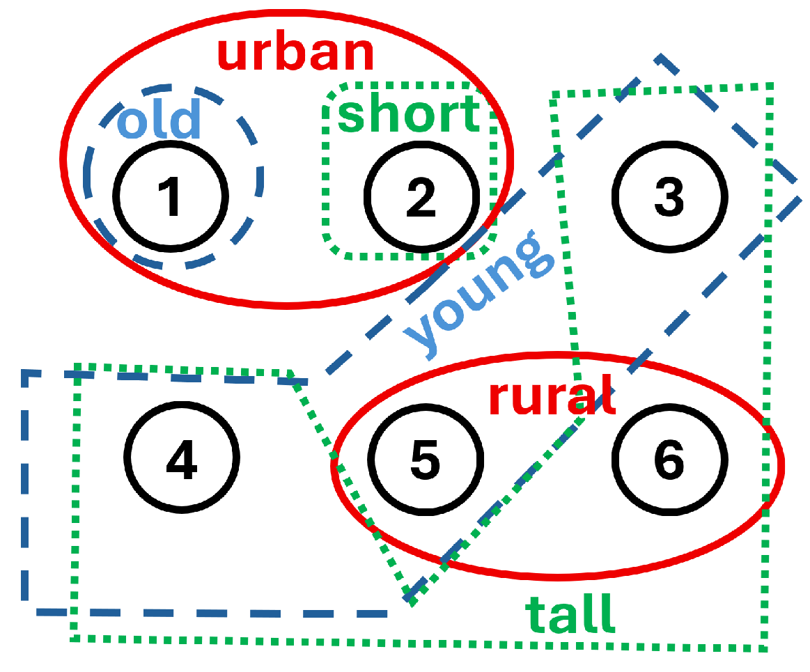
Each agent has exactly two traits, so . Set and , with all remaining lower quotas equal to zero and all upper quotas nonbinding. These lower quotas equal the expected trait counts rounded down, so the setting is consistent.
Every exactly diverse selected group contains exactly one agent from and three from . Indeed, the urban quota requires at least one of Agents 1 and 2. Selecting both would force the remaining two agents to be Agents 3 and 4 to satisfy the young and tall quotas, leaving the rural quota unsatisfied. Conversely, selecting one agent from and any three from satisfies every quota.
Consequently, every exactly diverse lottery satisfies . At least one of these agents therefore has selection probability at most , which is at least below the target .
By contrast, the uniform lottery over all groups of size four preserves every target probability exactly. Every group in its support violates each lower quota by at most one, so this lottery is 1-approximately diverse, consistent with the guarantee of Theorem 2.
The preferred lottery thus depends on the welfare components and their relative weights. A society placing sufficiently high weight on marginal preservation may prefer the uniform lottery, while a society prioritizing exact quota compliance may prefer an exactly diverse lottery.
References
- Budish, E.; Che, Y.-K.; Kojima, F.; Milgrom, P. Designing random allocation mechanisms: Theory and applications. Am. Econ. Rev. 2013, 103, 585–623. [Google Scholar] [CrossRef] [Scilit]
- Flanigan, B.; Gölz, P.; Gupta, A.; Hennig, B.; Procaccia, A.D. Fair algorithms for selecting citizens’ assemblies. Nature 2021, 596, 548–552. [Google Scholar] [CrossRef] [Scilit]
- Abdulkadiroğlu, A.; Sönmez, T. School choice: A mechanism design approach. Am. Econ. Rev. 2003, 93, 729–747. [Google Scholar] [CrossRef] [Scilit]
- Cohen-Schotanus, J.; Muijtjens, A.M.; Reinders, J.J.; Agsteribbe, J.; Van Rossum, H.J.; Van Der Vleuten, C.P. The predictive validity of grade point average scores in a partial lottery medical school admission system. Med. Educ. 2006, 40, 1012–1019. [Google Scholar] [CrossRef] [Scilit]
- Baum, L.E. State Laws on Weighted Lotteries and Enrollment Practices. Technical Report, National Alliance for Public Charter Schools; Prepared by the Law Office of Lauren E. Baum, PC and Civil Rights Solutions, LLC, 2015. Available online: https://publiccharters.org/wp-content/uploads/2023/01/NPC035_WeightedLotteries_Digital_rev.pdf (accessed on 26 October 2026).
- White, D.B.; McCreary, E.K.; Chang, C.-C.H.; Schmidhofer, M.; Bariola, J.R.; Jonassaint, N.N.; Persad, G.; Truog, R.D.; Pathak, P.; Sonmez, T.; et al. A multicenter weighted lottery to equitably allocate scarce COVID-19 therapeutics. Am. J. Respir. Crit. Care Med. 2022, 206, 503–506. [Google Scholar] [CrossRef] [Scilit]
- Flanigan, B.; Gölz, P.; Gupta, A.; Procaccia, A.D. Neutralizing self-selection bias in sampling for sortition. Adv. Neural Inf. Process. Syst. 2020, 33, 6528–6539. [Google Scholar]
- Beck, J.; Fiala, T. “Integer-making” theorems. Discret. Appl. Math. 1981, 3, 1–8. [Google Scholar] [CrossRef] [Scilit]
- Nguyen, T.; Peivandi, A.; Vohra, R. Assignment problems with complementarities. J. Econ. Theory 2016, 165, 209–241. [Google Scholar] [CrossRef] [Scilit]
- Gandhi, R.; Khuller, S.; Parthasarathy, S.; Srinivasan, A. Dependent rounding and its applications to approximation algorithms. J. ACM 2006, 53, 324–360. [Google Scholar] [CrossRef] [Scilit]
- Cembrano, J.; Correa, J.; Verdugo, V. Multidimensional political apportionment. Proc. Natl. Acad. Sci. USA 2022, 119, e2109305119. [Google Scholar] [CrossRef] [Scilit]
- Grimmett, G. Stochastic apportionment. Am. Math. Mon. 2004, 111, 299–307. [Google Scholar] [CrossRef] [Scilit]
- Correa, J.; Gölz, P.; Schmidt-Kraepelin, U.; Tucker-Foltz, J.; Verdugo, V. Monotone randomized apportionment. In Proceedings of the 25th ACM Conference on Economics and Computation; ACM Digital Library: New York, NY, USA, 2024; p. 71. [Google Scholar]
- Gölz, P.; Peters, D.; Procaccia, A.D. In this apportionment lottery, the house always wins. Oper. Res. 2026, 74, 390–407. [Google Scholar] [CrossRef] [Scilit]
- Ahuja, R.K.; Magnanti, T.L.; Orlin, J.B. Network Flows: Theory, Algorithms, and Applications; Prentice-Hall: Hoboken, NJ, USA, 1993. [Google Scholar]
- Aziz, H.; Brill, M.; Conitzer, V.; Elkind, E.; Freeman, R.; Walsh, T. Justified representation in approval-based committee voting. Soc. Choice Welf. 2017, 48, 461–485. [Google Scholar] [CrossRef] [Scilit]
- Aziz, H. A rule for committee selection with soft diversity constraints. Group Decis. Negot. 2019, 28, 1193–1200. [Google Scholar] [CrossRef] [Scilit]
- Bredereck, R.; Faliszewski, P.; Igarashi, A.; Lackner, M.; Skowron, P. Multiwinner elections with diversity constraints. In Proceedings of the AAAI Conference on Artificial Intelligence; Association for the Advancement of Artificial Intelligence: Washington, DC, USA, 2018; Volume 32. [Google Scholar]
- Mehrotra, A.; Pradelski, B.S.R.; Vishnoi, N.K. Selection in the presence of implicit bias: The advantage of intersectional constraints. In Proceedings of the 2022 ACM Conference on Fairness, Accountability, and Transparency; ACM Digital Library: New York, NY, USA, 2022; pp. 599–609. [Google Scholar]
- Ebadian, S.; Kehne, G.; Micha, E.; Procaccia, A.D.; Shah, N. Is sortition both representative and fair? Adv. Neural Inf. Process. Syst. 2022, 35, 3431–3443. [Google Scholar] [CrossRef] [Scilit]
- Baharav, C.; Flanigan, B. Fair, manipulation-robust, and transparent sortition. In Proceedings of the 25th ACM Conference on Economics and Computation; ACM Digital Library: New York, NY, USA, 2024; pp. 756–775. [Google Scholar]
- Assos, A.; Baharav, C.; Flanigan, B.; Procaccia, A.D. Alternates, assemble! selecting optimal alternates for citizens’ assemblies. In Proceedings of the 26th ACM Conference on Economics and Computation; ACM Digital Library: New York, NY, USA, 2025; pp. 719–738. [Google Scholar]
- Halpern, D.; Procaccia, A.D.; Shapiro, E.; Talmon, N. Federated assemblies. Proc. AAAI Conf. Artif. Intell. 2025, 39, 13897–13904. [Google Scholar] [CrossRef] [Scilit]
- Talmon, N.; Shapiro, E. Grassroots federation: Fair democratic governance at scale. In Proceedings of the 25th International Conference on Autonomous Agents and Multiagent Systems; ACM Digital Library: New York, NY, USA, 2026; pp. 1156–1164. [Google Scholar]
- de Azevedo, G.; Gölz, P. Maximally random sortition. arXiv 2026, arXiv:2604.02712. [Google Scholar]
- Hylland, A.; Zeckhauser, R. The efficient allocation of individuals to positions. J. Political Econ. 1979, 87, 293–314. [Google Scholar] [CrossRef] [Scilit]
- Bogomolnaia, A.; Moulin, H. A new solution to the random assignment problem. J. Econ. Theory 2001, 100, 295–328. [Google Scholar] [CrossRef] [Scilit]
- Akbarpour, M.; Nikzad, A. Approximate random allocation mechanisms. Rev. Econ. Stud. 2020, 87, 2473–2510. [Google Scholar] [CrossRef] [Scilit]
- Balbuzanov, I. Constrained random matching. J. Econ. Theory 2022, 203, 105472. [Google Scholar] [CrossRef] [Scilit]
- Han, X. A theory of fair random allocation under priorities. Theor. Econ. 2024, 19, 1185–1221. [Google Scholar] [CrossRef] [Scilit]
- Basteck, C.; Ehlers, L. On (constrained) efficiency of strategy-proof random assignment. Econometrica 2025, 93, 569–595. [Google Scholar] [CrossRef] [Scilit]
- Hafalir, I.E.; Yenmez, M.B.; Yildirim, M.A. Effective affirmative action in school choice. Theor. Econ. 2013, 8, 325–363. [Google Scholar] [CrossRef] [Scilit]
- Ehlers, L.; Hafalir, I.E.; Yenmez, M.B.; Yildirim, M.A. School choice with controlled choice constraints: Hard bounds versus soft bounds. J. Econ. Theory 2014, 153, 648–683. [Google Scholar] [CrossRef] [Scilit]
- Kamada, Y.; Kojima, F. Efficient matching under distributional constraints: Theory and applications. Am. Econ. Rev. 2015, 105, 67–99. [Google Scholar] [CrossRef] [Scilit]
- Kamada, Y.; Kojima, F. Stability and strategy-proofness for matching with constraints: A necessary and sufficient condition. Theor. Econ. 2018, 13, 761–793. [Google Scholar] [CrossRef] [Scilit]
- Kamada, Y.; Kojima, F. Fair matching under constraints: Theory and applications. Rev. Econ. Stud. 2024, 91, 1162–1199. [Google Scholar] [CrossRef] [Scilit]
- Carvalho, J.-P.; Pradelski, B.S.R.; Williams, C. Intersectionality: Affirmative action with multidimensional identities. Manag. Sci. 2025, 71, 4495–4509. [Google Scholar] [CrossRef] [Scilit]
- Learning Community Charter School. Weighted Lottery Information. 2026. Available online: https://www.lccsnj.org/admissions/weighted-lottery-information (accessed on 3 July 2026).
- Farrell, D.M.; Suiter, J. Reimagining Democracy: Lessons in Deliberative Democracy from the Irish Front Line; Cornell University Press: Ithaca, NY, USA, 2021. [Google Scholar]
- NYC. Affordable Housing Guide for Applicants with Disabilities. 2022. Available online: https://www.nyc.gov/assets/hpd/downloads/pdfs/services/affordable-housing-guide-for-applicants-with-disabilities.pdf (accessed on 4 July 2026).
- Diamond, S.S.; Hans, V.P.; Chizik, N.; Harfuch, A. The arrival of the civil jury in Argentina: The case of Chaco. Chic.-Kent Law Rev. 2024, 98, 167–192. [Google Scholar]
- Balinski, M.L.; Demange, G. An axiomatic approach to proportionality between matrices. Math. Oper. Res. 1989, 14, 700–719. [Google Scholar] [CrossRef] [Scilit]
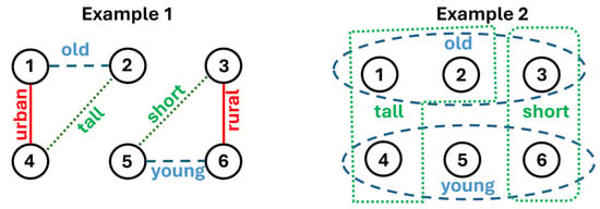
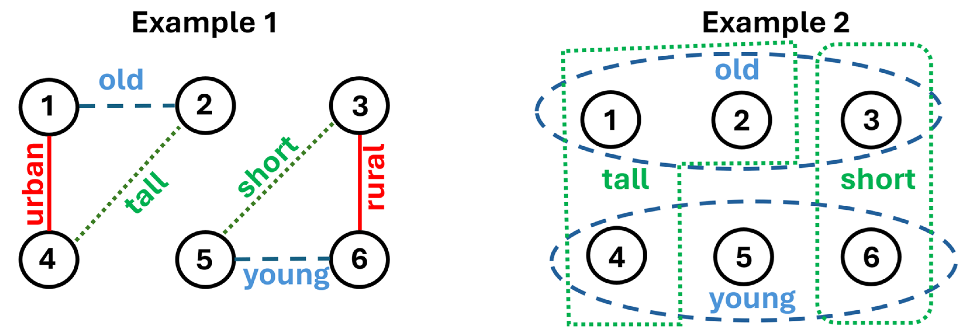
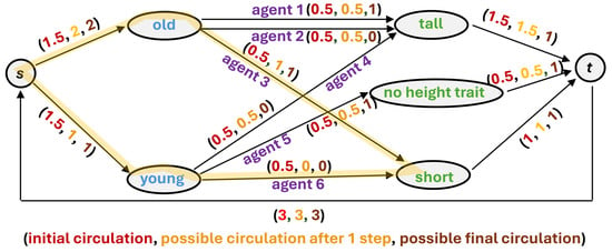
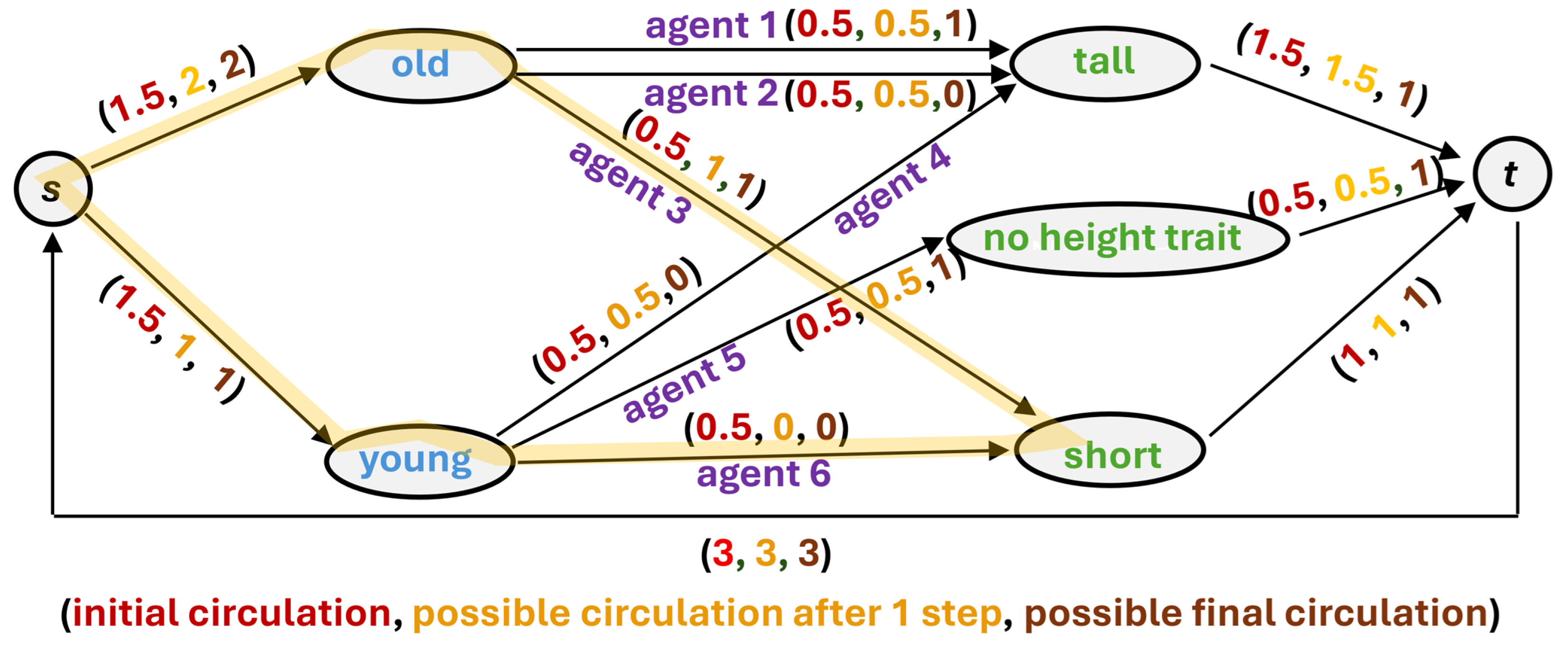

Disclaimer/Publisher’s Note: The statements, opinions and data contained in all publications are solely those of the individual author(s) and contributor(s) and not of MDPI and/or the editor(s). MDPI and/or the editor(s) disclaim responsibility for any injury to people or property resulting from any ideas, methods, instructions or products referred to in the content. |
© 2026 by the authors. Licensee MDPI, Basel, Switzerland. This article is an open access article distributed under the terms and conditions of the Creative Commons Attribution (CC BY) license.