


Abstract
Exploration quality and policy parameter updates influence the training of deterministic actor–critic controllers. This study presents ES–TD3, an evolution strategy-assisted Twin Delayed Deep Deterministic Policy Gradient framework that combines population-based actor-parameter search with off-policy learning. Candidate actors undergo Gaussian perturbation, episodic evaluation, elite selection, and fitness-weighted recombination. The mathematical analysis establishes that the recombined parameter vector lies within the convex hull of the elite actors and bounds its displacement from the current population center by the largest elite displacement, with a perturbation-dependent bound for Gaussian candidates. For a mass–spring–damper plant with positive mass, damping, and stiffness, bounded-input/bounded-state and Lyapunov analyses establish uniform ultimate boundedness of the physical state under the bounded deterministic actor output. These guarantees concern individual recombination steps and plant-state boundedness, not asymptotic tracking or global training convergence. MATLAB/Simulink simulations compare ES–TD3 with standard TD3 and PID control, examine reference and initial condition variations, and assess sensitivity to evolutionary settings. The best observed configuration reaches the moving-average reward threshold of 126,500 at generation 203 and attains a final moving-average reward of 126,512. The reported ES–TD3 run exhibits smoother reward progression than the TD3 baseline, while the deployed policy produces bounded tracking responses across the tested scenarios. The results support the feasibility of combining evolutionary policy search with actor–critic learning for the considered control problem; broader performance claims require independent repeated trials.
Keywords:
deep reinforcement learning; twin delayed deep deterministic policy gradient; evolution strategy; policy-space exploration; continuous control; hybrid optimization MSC:
68T05; 68W50; 93C15
1. Introduction
Continuous-control problems arise in many engineering applications in which a controller must generate smooth, real-valued actions while maintaining accurate tracking, stable transient behavior, and acceptable control effort. Classical methods, including proportional–integral–derivative (PID), state-space, optimal, adaptive, and robust controllers, remain effective when the system model and operating conditions are sufficiently well defined [1,2]. Vision-based control research has similarly combined complementary image-space and Cartesian-space information through probabilistic 2D/3D integration and has employed particle filtering to estimate target models required for visual servoing [3,4]. Recent developments continue to improve these approaches; for example, adaptive chattering-free sliding-mode control has been used to compensate for disturbances and uncertainties while maintaining continuous control inputs in robotic trajectory tracking [5]. Their performance, however, may deteriorate when the required model information is incomplete or when nonlinearities, parameter variations, uncertain dynamics, external disturbances, or actuator constraints are not adequately represented [6,7]. These challenges have motivated increasing interest in data-driven control methods that can learn control policies directly through interaction with a dynamic environment.
Reinforcement learning (RL) provides a general framework for learning sequential decision-making policies from sampled experience [8,9,10,11]. Unlike conventional model-based methods, RL does not necessarily require an exact analytical model of the controlled plant and can therefore be useful when the dynamics are difficult to derive, partially unknown, or time varying [12,13]. Related data-driven approaches have addressed unknown nonlinear dynamics through event-triggered model-free adaptive iterative learning control and have combined trajectory imitation with RL for complex continuous systems with sparse or difficult-to-specify rewards [14,15]. Perception-driven autonomy has also benefited from learned visual representations, including robust localization in highly crowded urban environments and deep-learning-based obstacle detection and avoidance for powered wheelchairs [16,17]. A more recent wheelchair navigation framework unifies CNN-based corridor following with image-based visual-servoing obstacle avoidance under a common perception-and-control architecture [18]. Deep RL has consequently been applied to a range of continuous-control tasks, including robotic manipulation, locomotion, visuomotor control, and embodied decision-making [19,20,21,22]. Recent control applications include RL-based motion planning for quadrotor navigation, real-time model-free stabilization of a quadruple inverted pendulum, and multi-actor–critic trajectory planning for robotic manipulators [23,24,25].
For continuous action spaces, actor–critic algorithms provide a practical mechanism for jointly learning a control policy and an approximation of its long-term value. Recent robust actor–critic control has combined learned policies with integral error feedback for perturbed mobile-robot tracking [26]. TD3 has also been formulated as an adaptive PID-like controller using error, integral-error, and derivative-error observations for uncertain mass–spring–damper dynamics [27]. Learning-based controllers can additionally be combined with model-derived structure: examples integrate deep RL with high-gain feedback or inverse dynamics [28,29], combine Pure Pursuit and PID control with TD3-based corrective actions for differential-drive robots [30], or use learned actors and critics to guide model predictive control optimization [31,32]. Twin Delayed Deep Deterministic Policy Gradient (TD3) extends deterministic policy-gradient learning through clipped double-Q estimation, delayed actor updates, and target policy smoothing [33]. These mechanisms reduce value overestimation and improve the stability of policy updates compared with earlier deterministic actor–critic methods such as DDPG [33,34]. Nevertheless, TD3 and related deep RL algorithms can remain sensitive to network initialization, reward scaling, random seeds, exploration noise, and hyperparameter selection [13,35,36]. Such sensitivity is particularly important in control applications, where inconsistent learning may produce oscillatory responses, excessive control actions, or policies that generalize poorly beyond the training conditions.
Exploration is commonly introduced in deterministic actor–critic methods by adding noise to the executed actions. Although action-space perturbation can support local exploration, it may be insufficient for discovering coordinated behavioral changes that require simultaneous modification of many policy parameters [37]. Guided exploration has recently been used in continuous-action pursuit–evasion, while structured artificial potential field information has been incorporated into DDPG to guide obstacle avoidance learning [38,39]. Parameter-space exploration offers an alternative by perturbing the policy representation itself, thereby producing temporally consistent changes in the actions generated over an entire episode. More broadly, reward-guided genetic evolution has been used to optimize lightweight policy-related adapter parameters for adaptive robot control without gradient updates [40]. Recent reviews similarly identify policy search, exploration, adaptation, and sample efficiency as central themes in evolutionary reinforcement learning [41]. Population-based evolutionary optimization extends this idea by evaluating multiple perturbed candidate policies, selecting high-performing individuals, and using their fitness values to guide the subsequent search process [42,43,44].
Evolution strategies, genetic algorithms, random search methods, and hybrid evolutionary reinforcement learning approaches have demonstrated that gradient-free policy search can be competitive in several continuous-control settings [45,46,47,48]. Pure evolutionary optimizers, however, do not exploit replay-based value learning and may require a large number of episodic policy evaluations when directly optimizing high-dimensional neural network parameters [42,44]. Conversely, gradient-based actor–critic algorithms can efficiently reuse previously collected experience but may remain dependent on local exploration and critic accuracy. Combining these two optimization paradigms therefore offers a means of exploiting the local policy-refinement capability of actor–critic learning together with the broader parameter-space search provided by population-based optimization.
Within this context, TD3 is selected as the reinforcement learning backbone because its off-policy formulation permits experience reuse, while its twin critics, delayed policy updates, and target smoothing provide an established basis for deterministic continuous control. The evolution strategy is introduced as an auxiliary search mechanism rather than as a replacement for gradient-based learning. The resulting framework perturbs the actor network parameters, evaluates a population of candidate policies according to episodic return, selects elite candidates, and constructs the next policy representation through fitness-weighted recombination. This design is intended to broaden policy-space exploration while retaining the replay-based learning and value estimation mechanisms of TD3. Although actor–critic reinforcement learning is closely related to adaptive dynamic programming (ADP), the proposed ES–TD3 framework differs from classical ADP-based optimal control schemes in the manner in which policy improvement is performed. ADP methods typically construct iterative approximations of the value function and control policy based on Bellman or Hamilton–Jacobi–Bellman formulations, often with theoretical analysis of admissibility and convergence under specific assumptions. In ES–TD3, the TD3 component performs model-free off-policy learning, while the evolutionary component perturbs and recombines actor parameters according to episodic fitness. These evolutionary operations do not constitute a Bellman-derived policy improvement operator and therefore do not imply monotonic policy improvement or convergence to the globally optimal controller.
The proposed framework is evaluated using continuous force control of a mass–spring–damper system. Such systems provide an interpretable benchmark for studying oscillatory dynamics, transient response, control effort, and tracking accuracy, and they approximate the behavior of several mechanical systems, including suspension components, actuators, structural vibration models, and simplified robotic mechanisms [1,2,6,7]. The benchmark therefore enables the effect of the evolutionary training mechanism to be examined under a controlled and reproducible simulation setting. This formulation differs from value iteration-based reinforcement learning approaches for unknown discrete-time systems, such as [49], which employ iterative value/policy updates within a discrete-time optimal control framework. In contrast, the present ES–TD3 framework uses model-free off-policy actor–critic learning and augments TD3 with evolutionary parameter-space exploration. The proposed method therefore addresses a different problem: broadening policy search in a continuous-action actor–critic setting rather than constructing a value iteration solution with corresponding optimality or admissibility guarantees.
The main contributions of this study are summarized as follows:
- An evolution strategy-assisted TD3 framework is developed in which Gaussian perturbations are applied directly to the actor network parameters, enabling policy-space exploration that complements conventional action-space noise.
- A structured coupling between evolutionary search and off-policy actor–critic learning is formulated through episodic candidate evaluation, replay-buffer updates, elite policy selection, and fitness-weighted parameter recombination.
- Formal properties of the framework are established by proving convex-hull containment and an elite radius displacement bound for the evolutionary update, together with uniform ultimate boundedness of the controlled plant under the bounded actor output.
- The proposed framework is evaluated against standard TD3 and PID control using learning behavior, threshold attainment performance, closed-loop tracking performance, and generalization across different reference signals and initial conditions.
- The influence of the main evolutionary design parameters, including population size, elite percentage, perturbation standard deviation, and returned policy selection, is examined through a systematic sensitivity analysis.
The remainder of this paper is organized as follows. Section 2 presents the theoretical background of reinforcement learning, TD3, evolution strategies, and the considered dynamic system. Section 3 describes the proposed ES–TD3 framework and its training procedure. Section 4 presents the experimental configuration, followed by the results, comparative evaluation, and sensitivity analysis. Finally, the main conclusions and directions for future research are discussed.
2. Background
2.1. Reinforcement Learning
Reinforcement learning formulates sequential decision making as a Markov decision process defined by the tuple , where and denote the state and action spaces, P represents the state transition dynamics, r is the reward function, and is the discount factor [8]. At time step t, an agent observes the state , selects an action according to a policy , receives a reward , and transitions to the next state .
The learning objective is to identify a policy that maximizes the expected discounted return
Deep reinforcement learning methods approximate the policy, value function, or both using neural networks. Actor–critic methods are particularly suitable for continuous-control problems because the actor generates real-valued actions while the critic estimates the expected return associated with state–action pairs [33,34]. Their practical performance, however, depends strongly on the accuracy of value estimation, the quality of exploration, and the stability of policy updates.
2.2. Twin Delayed Deep Deterministic Policy Gradient
Twin Delayed Deep Deterministic Policy Gradient is a model-free, off-policy actor–critic algorithm designed for continuous action spaces [33]. TD3 extends Deep Deterministic Policy Gradient by introducing three mechanisms intended to reduce value overestimation and unstable policy improvement: clipped double-Q learning, delayed actor updates, and target policy smoothing.
The algorithm maintains a deterministic actor , two critics and , and corresponding target networks. During environment interaction, the action is generated as
where denotes exploration noise applied to the executed action. The resulting transition is stored in a replay buffer .
For a mini-batch sampled from , the target action is computed using the target actor and clipped smoothing noise:
The corresponding TD target is
and each critic is updated by minimizing
The actor is updated less frequently than the critics using the deterministic policy gradient
The target networks are then updated through Polyak averaging:
The use of the minimum of two critic estimates limits optimistic value bias, delayed actor updates reduce the effect of rapidly changing critic estimates, and target policy smoothing discourages exploitation of narrow peaks in the learned value function [33,34]. Figure 1 summarizes the TD3 learning process used as the reinforcement learning backbone of the proposed framework.
Figure 1.
Overview of the TD3 learning process used as the reinforcement learning backbone of the proposed framework: (A) environment interaction and experience replay; (B) target construction and separate critic updates; and (C) delayed actor and soft target updates. Solid arrows indicate data flow, whereas dashed arrows indicate parameter updates. Colors distinguish functional components only.
2.3. Evolution Strategies
Evolution strategies are population-based, gradient-free optimization methods that search over a parameterized solution space through stochastic sampling, performance evaluation, selection, and distribution updates [42,43,44]. When applied to reinforcement learning, the optimized solution is commonly the parameter vector of a policy network.
Let denote the parameters of a policy. A population of N candidate policies can be generated by Gaussian perturbation:
where controls the scale of parameter-space exploration. Each candidate policy is evaluated in the environment using an episodic fitness measure such as cumulative reward:
The fitness values are then used to select or weight high-performing candidates when constructing the next search distribution. Unlike action-space noise, which perturbs individual actions during interaction, evolution strategies perturb the policy parameters and therefore induce temporally consistent behavioral changes over an entire episode. This property makes evolutionary search a useful complement to deterministic actor–critic learning, particularly when local action perturbations provide limited exploration of the policy space.
2.4. Mass–Spring–Damper System Model
The controlled plant is represented, as shown in Figure 2, by a single-degree-of-freedom mass–spring–damper system. This model is widely used as an interpretable benchmark for vibration analysis, transient-response evaluation, and controller assessment in mechanical systems [1,7]. It captures the interaction among inertia, elastic restoring force, viscous damping, and external actuation while remaining analytically tractable.
Figure 2.
Single-degree-of-freedom mass–spring–damper system considered in the continuous-control environment. Here, m denotes the mass, k the spring stiffness, c the viscous damping coefficient, x the displacement from equilibrium, and f the applied control force.
Let denote the displacement of the mass, its velocity, and the control force generated by the agent. The plant dynamics are described by
where m, c, and k denote the mass, damping coefficient, and spring stiffness, respectively.
Using the state variables
the system can be written in first-order form as
In the reinforcement learning environment, the policy maps the observation vector to a bounded continuous force command. The control objective is to track a prescribed reference while limiting oscillation, steady-state error, transient duration, and excessive control effort. The complete observation representation, action bounds, reward formulation, and simulation parameters are specified in the subsequent sections.
3. Proposed ES–TD3 Framework
3.1. Framework Overview
The proposed framework combines gradient-based TD3 learning with population-based evolution strategy search. The TD3 component performs off-policy actor–critic learning using transitions stored in a replay buffer, whereas the evolutionary component explores the actor-parameter space through Gaussian perturbation, episodic policy evaluation, elite selection, and fitness-weighted recombination.
The overall ES–TD3 workflow is illustrated in Figure 3. At generation g, the actor parameter vector defines the center of the evolutionary search distribution. A population of candidate actors is generated by perturbing . Each candidate is evaluated for one complete episode in the Simulink environment, and the resulting transitions are stored in a shared replay buffer . The episodic return of each candidate is used as its fitness value.
Figure 3.
Overall workflow of the proposed ES–TD3 framework: (A) candidate interaction with the Simulink mass–spring–damper environment and transition storage; and (B) evolutionary actor search coupled with replay-based TD3 learning. Candidate actors are generated through Gaussian perturbation, evaluated by episodic return, and selected for fitness-weighted recombination. Shared replay transitions support TD3 critic learning and actor refinement. Solid arrows indicate data and workflow; the dashed arrow indicates gradient-based actor refinement.
After evaluating the population, the TD3 critics and actor are updated using mini-batches sampled from the shared replay buffer. The candidate policies are then ranked according to their episodic returns, and the best-performing candidates are retained as elites. Their actor parameters are combined using fitness-weighted recombination, and the resulting parameter vector defines the center of the search distribution for the next generation.
This coupling enables the critic networks to learn from trajectories generated by multiple neighboring policies, while the evolutionary process explores actor-parameter regions that may not be reached through action-space noise alone.
3.2. Observation and Action Representation
At time step t, the agent receives an observation vector
where denotes the system position, is the linear velocity, r is the reference input, is the tracking error, is the time derivative of the tracking error, and represents the accumulated tracking error.
Based on this observation, the deterministic actor generates the continuous control force
where denotes the trainable actor parameters. The actor output is processed by a hyperbolic tangent activation function and an action scaling layer so that the applied force satisfies
where is the unscaled actor output and is the force-scaling coefficient.
The observation vector combines the plant-state and reference tracking variables required by the controller. Their definitions, physical units, network input treatment, and the numerical action bounds are reported in Section 4.2.
3.3. TD3 Agent Architecture
The TD3 agent is implemented using the MATLAB R2025b Reinforcement Learning Toolbox [50]. It consists of one deterministic actor network, two critic networks, and their corresponding target networks. The two critics estimate the action-value functions and .
The actor and critic networks use fully connected architectures with two hidden layers containing 400 and 300 neurons, respectively. Rectified linear unit activation functions are used in the hidden layers. The actor generates a deterministic continuous output through a hyperbolic tangent layer followed by an action scaling layer.
Each critic receives the observation and action as inputs and produces a scalar Q-value estimate. The observation and action pathways are processed separately in the initial layers and are subsequently combined before the final Q-value output.
The actor and critic networks are optimized using Adam with a learning rate of
The mini-batch size and discount factor are set to
respectively.
During environment interaction, action-space exploration is introduced by adding Ornstein–Uhlenbeck noise to the deterministic actor output:
where is generated by the Ornstein–Uhlenbeck process. This noise perturbs the executed actions and is distinct from the Gaussian parameter perturbations introduced by the evolution strategy component.
Target policy smoothing is applied during critic learning. The target action is computed as
where denotes the target actor parameters. The target smoothing noise parameter is set to 0.2 in the present implementation.
For a transition , the critic target is calculated as
where is the terminal-state indicator. Each critic is updated by minimizing
The actor is updated less frequently than the critics using the deterministic policy gradient
The target networks are updated through Polyak averaging:
3.4. Evolution Strategy-Based Policy Search
Let denote the actor parameter vector at generation g, where d is the total number of trainable actor weights and biases. A population of N candidate actors is generated by perturbing the current actor parameters:
where determines the magnitude of exploration in the actor-parameter space. Equivalently,
The perturbations are applied to both actor weights and biases. Since the perturbed parameters remain fixed throughout a candidate episode, each candidate produces a temporally consistent behavioral variation. This differs from action-space exploration, which independently modifies the force commands generated during interaction.
Each candidate actor is evaluated for one episode in the Simulink environment. Its fitness is defined as the undiscounted cumulative episodic reward:
where is the episode length of candidate i and is its instantaneous reward.
During candidate evaluation, each transition is stored in the shared replay buffer:
After all candidates have been evaluated, they are ranked in descending order of fitness. For an elite ratio , the number of elite candidates is
The elite set is defined as
where rank 1 identifies the candidate with the highest episodic fitness.
Because the magnitude and sign of episodic returns may vary, the elite fitness values are shifted to obtain nonnegative recombination scores:
where is a small numerical constant. The normalized fitness-based weight assigned to elite candidate i is
with
The recombined actor parameter vector is then calculated as
The recombined actor is subsequently used as the center of the search distribution for the next generation.
3.5. Coupling of Evolutionary Search and TD3 Learning
The evolutionary and TD3 components are coupled through a shared replay buffer and a common population-based actor representation. The implementation uses trainWithEvolutionStrategy with an rlTD3Agent and the weighted-mixing population-update method. At each generation, the following sequence is applied:
- Generate N candidate actors by perturbing the current population center in the actor-parameter space.
- Evaluate each candidate actor for one complete episode and store the resulting transitions in the shared replay buffer .
- Perform K gradient-based TD3 training epochs using mini-batches sampled from . The critic, actor, and target-network updates follow the standard delayed TD3 learning procedure.
- Rank the evaluated actors according to their episodic fitness and select the elite subset .
- Construct the actor representation used for the next population through fitness-weighted elite mixing:
The MATLAB implementation therefore does not apply a TD3 actor-gradient step and then unconditionally overwrite that actor with an independently computed ES solution. Instead, the gradient-based TD3 actor participates in the population-based procedure and contributes to the next weighted-mixing update only when it is selected among the elite actors according to its episodic fitness. The critic networks are not subjected to evolutionary perturbation; they are updated only through replay-based TD3 learning.
No explicit hard synchronization of the target actor is performed after the weighted-mixing step. The target actor continues to be updated through the standard Polyak averaging rule in Equation (23), with in the MATLAB implementation.
The principal training configuration uses a maximum of 500 generations, a population size of , an elite ratio of , and an initial perturbation standard deviation of . Each candidate is evaluated once per generation, and TD3 training epochs are performed within each generation.
3.6. Analytical Properties of Evolutionary Updates and Closed-Loop Boundedness
This subsection establishes two properties that follow from the implemented ES–TD3 structure. The first concerns the geometry and magnitude of the fitness-weighted evolutionary update. The second concerns boundedness of the physical plant under the bounded deterministic actor output. These results do not require the critic approximation to be exact and do not assert global convergence of the nonconvex actor–critic training problem. Accordingly, the evolutionary update should be interpreted as a heuristic parameter-space search mechanism rather than as an ADP-type policy improvement operator with guaranteed monotonic performance improvement.
In this context, Proposition 1 characterizes an algorithm-specific property of the ES–TD3 evolutionary update, whereas Theorem 1 characterizes a plant-level bounded-input/bounded-state property that is not specific to the ES–TD3 learning algorithm.
Assumption 1.
The physical parameters satisfy , , and .
Assumption 2.
During deterministic evaluation and deployment, the applied control is the scaled actor output in Equation (14); hence . The reference signal is bounded, .
Proposition 1
Proof.
Because , every shifted elite score in Equation (30) is strictly positive. Normalization in Equation (31) therefore gives positive weights whose sum is one. Equation (33) is thus a convex combination of the elite parameter vectors. Furthermore, the triangle inequality and normalization of the weights give
which proves Equation (36). Substitution of Equation (24) gives Equation (37). □
Proposition 1 shows that weighted mixing cannot place the new population center outside the convex hull of the selected actors and that its displacement cannot exceed the largest elite displacement. For a population consisting of Gaussian perturbations, the perturbation scale directly bounds the realized update through Equation (37). Because the neural policy fitness is nonconvex, this geometric property does not imply monotonic improvement of episodic return.
Theorem 1
(Closed-loop state boundedness). Under Assumptions 1 and 2, the mass–spring–damper state is bounded for every finite initial condition. More precisely, there exist constants and such that
where
Thus, the state is uniformly ultimately bounded. If the reference is bounded, then the tracking error is also bounded because .
Proof.
The characteristic polynomial of is
Under Assumption 1, both coefficients are positive, so the second-order Routh–Hurwitz criterion implies that is Hurwitz. Therefore, constants and exist such that . The variation-of-constants formula gives
Applying Assumption 2 and the exponential matrix bound yields Equation (41). Taking the limit superior gives
which establishes uniform ultimate boundedness. □
For the numerical plant used in this study, , , and , the eigenvalues are , which confirms that the unforced plant is exponentially stable. An explicit Lyapunov certificate is
With and any , Young’s inequality gives
This provides a second, constructive certificate of ultimate boundedness for the implemented plant. The bound is deliberately worst-case because it uses only the action limit and does not use the observed tracking quality of the trained policy.
Remark 1.
Theorem 1 guarantees bounded plant trajectories under Assumptions 1 and 2. This boundedness property follows from the Hurwitz plant dynamics together with the bounded control input and is therefore not an algorithm-specific stability guarantee of ES–TD3. The algorithm-specific role is limited to enforcing the bounded control action through the scaled hyperbolic-tangent actor output. The theorem does not establish asymptotic tracking, monotonic reward improvement, policy optimality, or global convergence of TD3 or ES–TD3.
For a bounded reference signal satisfying , the tracking error satisfies
Hence,
This bound establishes bounded tracking error but does not imply . Therefore, the present analysis does not provide an asymptotic tracking guarantee for ES–TD3.
3.7. Reward Function
Let denote the reference signal and the displacement of the mass at time step t. The tracking error is defined as
The Simulink environment also uses a binary displacement constraint indicator. The admissible displacement interval is ; therefore,
In addition, a small-error indicator is defined as
Based on the Simulink implementation, the instantaneous reward is written as
where denotes the control force generated by the agent. The first term penalizes the squared tracking error and therefore provides dense feedback for reference tracking. The second term penalizes the squared control action to discourage unnecessarily large control effort. The third term imposes a substantially larger penalty when the displacement violates the admissible interval. The final term provides an additional positive reward when the absolute tracking error enters the small-error region .
The displacement constraint signal also activates the Simulink stop-simulation subsystem, so an episode terminates when or . Importantly, the penalty coefficient itself does not directly terminate the episode; termination is triggered by the displacement constraint condition. Nevertheless, the relative magnitudes of the reward coefficients can substantially affect the learning signal and training behavior. In particular, an excessively large constraint penalty may dominate the reward received near constraint violations, whereas an insufficient penalty may provide inadequate discouragement of such behavior. The reward coefficients were therefore selected empirically as task-specific design parameters rather than as theoretically optimal weights.
Preliminary Reward-Coefficient Study
To inform the selection of the tracking error and displacement constraint penalties, five preliminary reward-coefficient configurations were evaluated. The selection criterion was the predefined moving-average reward threshold of 126,500 in Equation (69). As summarized in Table 1, configuration R3, with an error penalty coefficient of 100 and a constraint penalty coefficient of 500, was the only tested configuration to attain this threshold. The other four tested configurations did not attain it. These pilot results motivate the coefficient pair used in the principal configuration; they are not an exhaustive search and do not establish that this pair is globally optimal.
Table 1.
Preliminary evaluation of reward-penalty coefficients.
The reward coefficients also influence the balance between tracking accuracy and constraint enforcement during training. An excessively large displacement constraint penalty may dominate the reward signal and reduce the relative contribution of the tracking objective, which can adversely affect training stability. Moreover, when displacement constraint violations are coupled with an episode-termination condition, such violations may lead to prematurely terminated episodes and consequently reduce the amount of trajectory information available for policy improvement. Conversely, a constraint penalty that is too small may provide insufficient discouragement of undesirable state excursions. The selected coefficients therefore represent an empirical trade-off between tracking performance and constraint enforcement within the tested configurations. These preliminary experiments are intended to motivate the adopted reward design and should not be interpreted as an exhaustive optimization of the reward coefficients.
3.8. Complete Training Procedure
Algorithm 1 summarizes the implementation-consistent ES–TD3 training procedure.
| Algorithm 1 Evolution Strategy-Assisted TD3 Training Procedure |
|
In the reported configuration,
and the stopping threshold is
The training process terminates when the moving-average reward reaches the specified threshold or when the maximum number of generations is completed. The best-performing candidate actor is retained as the final policy.
For reproducibility, K denotes the number of gradient-based TD3 training epochs performed per evolutionary generation. In the MATLAB implementation, this value is specified by the TrainEpochs property of rlEvolutionStrategyTrainingOptions and is set to
Each training epoch corresponds to one replay-buffer mini-batch update cycle with mini-batch size . Consequently, five mini-batch update cycles are performed per evolutionary generation. The twin critics are updated from these mini-batches, whereas actor and target-network updates follow the delayed TD3 update schedule and Polyak-averaging mechanism implemented by the MATLAB rlTD3Agent.
4. Experimental Setup
4.1. Simulation Environment
The proposed ES–TD3 controller was implemented in MATLAB R2025b using Simulink and the Reinforcement Learning Toolbox. The simulation environment represents the single-degree-of-freedom mass–spring–damper system described in Section 3. At each decision step, the agent receives the observation vector, generates a bounded continuous force command, and applies it to the plant. The environment then returns the next observation, instantaneous reward, and episode-termination signal.
From the learning perspective, the controller is model-free: the actor and critic networks do not use the analytical plant dynamics or the physical parameters m, c, and k during policy learning. Instead, training is based on sampled state–action–reward–next-state transitions generated by the Simulink environment. The plant model and its physical parameters are used only to construct the simulation environment and in the subsequent theoretical boundedness analysis.
Each episode has a simulation duration of
with a sampling interval of
Accordingly, the maximum number of interaction steps per episode is
An episode terminates when either the complete simulation horizon is reached or the displacement violates the admissible interval
Thus, early termination is activated when
4.2. Plant, Observation, and Action Configuration
The controlled plant is represented by
where m, c, and k denote the mass, viscous damping coefficient, and spring stiffness, respectively, and is the continuous control force generated by the agent.
The numerical plant parameters used in the Simulink model are summarized in Table 2.
Table 2.
Mass–spring–damper plant and simulation parameters.
At time step t, the actor receives the six-dimensional observation vector
where is the displacement of the mass, is its linear velocity, r is the reference displacement, is the tracking error, is the tracking error derivative, and is the accumulated tracking error.
The physical interpretation and units of the observation variables are reported in Table 3. It is worth noting that no explicit normalization is applied before the observations are provided to the actor network.
Table 3.
Observation and action definitions used in the Simulink environment.
The deterministic actor produces the control force
A hyperbolic tangent output layer followed by an action-scaling layer constrains the applied force to
4.3. Reward and Episode-Termination Configuration
The tracking error is defined as
The reward implemented in the Simulink environment is defined in Equation (53), using the coefficients identified in the preliminary study in the subsection entitled “Preliminary Reward-Coefficient Study”. The binary displacement constraint indicator is
The tracking error term provides dense feedback, while the constraint term penalizes excursions outside the admissible displacement interval. The small-error bonus and control-effort term are also included as specified in Equation (53). When the displacement constraint is violated, the Simulink stop-simulation subsystem terminates the episode. Accordingly, the constraint penalty is part of the reward signal, whereas termination is triggered by the displacement constraint logic. The selected coefficients should be interpreted as task-specific empirical settings, not as globally optimal values.
4.4. Network and Learning Configuration
The TD3 agent consists of one deterministic actor, two critic networks, and their corresponding target networks. The actor and critic networks use two fully connected hidden layers containing 400 and 300 neurons, respectively, with rectified linear unit activation functions. The actor output is processed by a hyperbolic tangent activation function followed by the action-scaling layer.
The actor and critic networks are optimized using Adam. The principal TD3 and evolutionary training settings are summarized in Table 4.
Table 4.
Principal ES–TD3 training parameters.
The controller is trained using trainWithEvolutionStrategy with an rlTD3Agent. The evolutionary training options specify
After the candidate population is evaluated in each generation, five replay-buffer mini-batch update cycles are conducted using a mini-batch size of 128. The critics are updated according to the TD3 learning rule, while actor and target-network updates follow the delayed-update and Polyak-averaging mechanisms implemented by the MATLAB rlTD3Agent.
The population update is configured by assigning “WeightedMixing” to the MATLAB UpdateMethod option. Gaussian perturbations with an initial standard deviation of 0.005 are applied to both the weights and biases of the actor network. Each generation contains 35 candidate actors, and the highest-performing 50% are retained for fitness-weighted recombination.
4.5. Stopping and Policy-Selection Criteria
Training terminates when either the maximum limit of 500 generations is reached or the moving-average reward satisfies
The moving average is computed using a window of 10 episodes. The BestPolicy returned policy option is used in the principal experiment, and the best-performing candidate is retained as the final trained controller.
The target value of 126,500 was selected empirically through preliminary trial-and-error simulations based on the reward levels observed during early training runs. It was not derived from a theoretical reward limit. Accordingly, the value was used as a practical performance threshold for identifying and retaining the best-performing policy rather than as an analytically computed upper bound.
4.6. Baseline and Evaluation Protocol
The proposed ES–TD3 framework is compared with standard TD3 trained without the evolutionary actor-parameter search mechanism. The TD3-only baseline uses the same plant model, observation vector, action space, reward function, simulation horizon, sampling interval, and network architecture. This comparison is used to isolate the effect of population-based parameter-space exploration.
Standard TD3 was selected as the principal learning baseline because the proposed method directly extends TD3, allowing the effect of the evolutionary parameter-space search mechanism to be isolated under otherwise identical training conditions. In this sense, the TD3 comparison serves as a controlled ablation-style baseline for evaluating the contribution of the proposed ES component.
The trained ES–TD3 policy is also compared with a conventional PID controller. The PID gains are adopted from [51].
The evaluation considers three aspects. First, training behavior is assessed using episodic reward, moving-average reward, generation at termination, final average reward, and training time. Second, the closed-loop tracking response of the trained ES–TD3 policy is compared with that of the PID controller. Third, generalization is examined using reference signals and initial conditions that differ from those used in the principal training experiment.
A closer evolutionary or hybrid reinforcement learning baseline was not included in the present study. Such methods may differ simultaneously in population-update rules, policy architectures, replay mechanisms, or training budgets, making a controlled one-factor comparison with the proposed ES component less direct. A broader comparison with evolutionary and hybrid RL methods is therefore identified as an important direction for future work.
4.7. Hyperparameter Sensitivity Protocol
A one-factor-at-a-time sensitivity analysis is conducted to examine the influence of the principal evolutionary design parameters. One parameter is varied in each experiment while the remaining settings are fixed at their principal values in Table 4. The investigated values are summarized in Table 5.
Table 5.
Hyperparameter values evaluated in the sensitivity analysis.
All sensitivity configurations use the same target average reward of 126,500 and the same maximum limit of 500 generations. The configurations are compared in terms of generation at threshold attainment, final average reward, training time, and satisfaction of the stopping criterion. All hyperparameter-sensitivity experiments were conducted using the same fixed random seed (Seed 0) to provide a controlled comparison among configurations; therefore, the reported trends should be interpreted as seed-specific exploratory observations rather than statistically robust estimates of hyperparameter effects. The separate multi-seed analysis presented in Section 5.2 further demonstrates that ES–TD3 training is sensitive to random initialization. Accordingly, the relative ranking of the tested hyperparameter configurations should not be interpreted as a statistically stable ordering across random seeds.
4.8. Computational Platform
All simulations were conducted on a Mac mini equipped with an Apple M4 Pro processor comprising a 12-core CPU and a 16-core GPU, together with 48 GB of unified memory. The implementation used MATLAB R2025b, Simulink, and the MATLAB Reinforcement Learning Toolbox.
5. Results and Discussion
5.1. Training Performance
Figure 4 presents the episodic reward and the moving-average reward obtained using the principal ES–TD3 configuration. The moving-average reward progressively increases during training and reaches the predefined stopping threshold of 126,500 at generation 203. Training is therefore terminated before the maximum limit of 500 generations is exhausted. The final moving-average reward is 126,512, and the corresponding training time is 0.9 h.
Figure 4.
Training performance of the proposed ES–TD3 agent. The moving-average reward reaches the predefined threshold of 126,500 at generation 203, after which the training process terminates automatically.
The reward trajectory indicates an overall improvement in the policy during the evolutionary training process, although short-term variations remain in the episodic returns. The attainment of the stopping threshold confirms that the principal configuration satisfies the predefined training criterion within the specified generation limit. However, this outcome should be interpreted as the result of the reported configuration and training run rather than as evidence that the selected hyperparameters are globally optimal.
5.2. Multi-Seed Training Performance
Figure 5 presents the episodic returns and corresponding moving-average returns obtained from ES–TD3 training runs with three different random seeds.
Figure 5.
Episodic and moving-average returns for ES–TD3 training runs with three different random seeds.
Of the three runs, only Seed 0 attains the predefined stopping threshold. Seeds 1 and 2 do not satisfy this criterion within the 500-generation training limit. These results indicate variability in threshold attainment across the tested random seeds and do not establish consistent threshold attainment across repeated runs.
Table 6 reports the per-seed training outcomes and the mean and standard deviation across the three runs.
Table 6.
Performance summary of ES–TD3 across three random seeds.
5.3. Comparison with Standard TD3
Figure 6 presents the training reward and moving-average reward obtained using standard TD3 without the evolution strategy-assisted actor-parameter search mechanism. The TD3-only baseline uses the same plant model, observation vector, action space, reward function, simulation duration, sampling interval, and neural network architecture as the proposed framework.
Figure 6.
Training reward and moving-average reward obtained using standard TD3 without evolution strategy-assisted parameter-space exploration.
In the reported run, the TD3-only baseline exhibits larger fluctuations in the episodic reward and a less consistent moving-average trajectory. Although the moving-average reward improves after the initial training phase, it does not reach the predefined threshold within the maximum limit of 500 generations. By comparison, ES–TD3 reaches the same threshold at generation 203.
This comparison provides initial evidence that the addition of population-based actor-parameter exploration may improve the consistency of the training process for the considered continuous-control problem. However, because the comparison is based on the reported training runs rather than on a multi-seed statistical evaluation, the observed difference should not be interpreted as a general guarantee of superior threshold attainment or stability.
5.4. Closed-Loop Comparison with PID Control
The closed-loop response of the trained ES–TD3 policy is compared with that of a conventional PID controller in Figure 7. The PID gains are adopted from the reinforcement learning-based PID tuning study reported in [51]. Both controllers are evaluated using the same mass–spring–damper plant and reference tracking scenario.
Figure 7.
Closed-loop response comparison between the trained ES–TD3 controller and the PID controller whose gains are adopted from [51].
The responses in Figure 7 show that both controllers produce bounded closed-loop trajectories and ultimately track the reference signal. The PID controller exhibits a smaller transient excursion below the reference, whereas the ES–TD3 controller shows a larger initial undershoot but enters the settling band earlier. Because the response starts above the reference and crosses below the target during the transient phase, the dominant transient excursion is characterized as undershoot rather than conventional positive overshoot.
Table 7 summarizes the quantitative closed-loop tracking performance of both controllers. In addition to the previously reported final tracking error, mean absolute error (MAE), root mean square error (RMSE), and maximum absolute error, the revised comparison includes the integral absolute error (IAE), maximum transient undershoot, and settling time. The settling time is defined as the earliest time after which the response remains within a band of the commanded position change around the reference.
Table 7.
Quantitative closed-loop tracking comparison between the PID and ES–TD3 controllers.
The quantitative results indicate a trade-off between transient deviation and settling behavior. The PID controller exhibits a smaller IAE and substantially smaller maximum undershoot, indicating lower overall transient deviation in the reported scenario. In contrast, the ES–TD3 controller enters the defined settling band earlier and achieves a smaller final tracking error. Therefore, the results do not indicate uniform superiority of either controller; rather, they reveal different transient and steady-state performance characteristics. A direct control-effort comparison is not reported because the available evaluation records contain the position and reference trajectories but do not include the complete control-input histories required for a consistent control-effort calculation.
5.5. Evaluation Under Varying Reference Signals and Initial Conditions
The behavior of the trained ES–TD3 policy is further examined under reference signals and initial conditions that differ from the principal training scenario. Figure 8 presents the corresponding closed-loop responses.
Figure 8.
Tracking performance of the trained ES–TD3 policy under different reference signals and initial conditions.
The policy remains bounded and follows the reference trajectories in the illustrated cases. These experiments provide an initial indication that the trained controller is not restricted to a single reference signal or initial state within the tested operating range.
However, these tests provide only a limited assessment of generalization and should not be interpreted as a comprehensive robustness analysis. In particular, robustness with respect to plant-parameter uncertainty, external disturbances, and measurement noise has not been established in the present study. A more comprehensive robustness assessment would require dedicated experiments under such perturbations, together with quantitative performance metrics for each condition. These aspects are therefore left for future work.
5.6. Hyperparameter Configuration Study
Because the complete sensitivity grid was evaluated using a single fixed random seed, the observed ranking of hyperparameter settings should be interpreted as exploratory and configuration-specific rather than as a statistically robust ordering across random initializations. A one-factor-at-a-time configuration study is conducted to examine the observed influence of the principal evolutionary parameters. For each experiment, one parameter is varied while the remaining settings are fixed at the principal values reported in Table 4. The configurations are compared in terms of threshold attainment, generation at threshold, final moving-average reward, and training time.
Each table reports the outcome of the corresponding training run. Because independent repeated runs with different random seeds were not conducted, the results should be interpreted as configuration-specific observations rather than as statistical estimates of hyperparameter effects.
The principal configuration is
This same reference run appears in the population-size, elite-percentage, initial-standard-deviation, and returned policy tables. Consequently, the repeated result of generation 203, a final moving-average reward of 126,512, and a training time of 0.9 h corresponds to the same principal experiment and should not be interpreted as four independent replications.
5.6.1. Population Size
Population size determines the number of candidate actor policies evaluated during each evolutionary generation. A larger population may provide broader parameter-space exploration, but it also increases the number of complete episode evaluations required per generation.
Table 8 presents the results obtained using population sizes between 15 and 65. The stopping threshold is fixed at a moving-average reward of 126,500, and all configurations are allowed to run for a maximum of 500 generations.
Table 8.
Effect of population size on ES–TD3 training. “Not attained” indicates that the moving-average reward threshold was not attained within 500 generations.
Among the evaluated population sizes, only reaches the predefined threshold within 500 generations. Smaller populations require less population-level evaluation per generation but remain below the target reward in the reported runs. Larger populations increase the observed training time without reaching the stopping threshold.
Therefore, provides the strongest observed result among the tested population sizes for this experimental configuration. The training times are not strictly monotonic with population size, which may reflect differences in episode termination, execution overhead, and hardware utilization during the individual runs.
5.6.2. Elite Percentage
The elite percentage determines the fraction of the highest-performing candidate actors retained during the weighted-mixing population update. A smaller elite fraction applies stronger selection pressure, whereas a larger fraction preserves a broader set of candidate solutions.
Table 9 summarizes the results obtained for elite percentages from 10% to 60%.
Table 9.
Effect of elite percentage on ES–TD3 training. “Not attained” indicates that the moving-average reward threshold was not attained within 500 generations.
Among the evaluated elite percentages, the 50% setting is the only configuration that reaches the stopping threshold. The 20% setting obtains the second-highest final moving-average reward but remains below the target after 500 generations. The remaining settings produce lower final rewards in the reported runs.
These results indicate that an elite percentage of 50% provides the strongest observed outcome for the current population size and perturbation scale. However, because each setting is represented by a single run, the results do not establish a general optimal selection ratio.
5.6.3. Initial Perturbation Standard Deviation
The initial perturbation standard deviation controls the magnitude of the Gaussian perturbations applied to the actor weights and biases. Small values produce candidate policies close to the current search center, whereas larger values explore more distant regions of the actor-parameter space.
Table 10 presents the results obtained using initial standard deviations of 0.001, 0.005, 0.01, and 0.05.
Table 10.
Effect of the initial perturbation standard deviation on ES–TD3 training. “Not attained” indicates that the moving-average reward threshold was not attained within 500 generations.
Only reaches the predefined moving-average reward threshold. The smaller value of 0.001 and the larger values of 0.01 and 0.05 remain below the target within the maximum generation limit.
The results indicate that the training outcome is sensitive to the initial perturbation scale. Among the evaluated values, provides the best observed balance between local policy refinement and broader parameter-space exploration. This conclusion is limited to the considered plant, network architecture, population size, and training configuration.
5.6.4. Returned Policy Option
The returned policy option determines which actor representation is retained after the evolutionary training procedure. Two MATLAB options are evaluated: BestPolicy and AveragedPolicy.
Table 11 presents the corresponding results.
Table 11.
Effect of the returned policy option on ES–TD3 training. “Not attained” indicates that the moving-average reward threshold was not attained within 500 generations.
The BestPolicy option reaches the stopping threshold at generation 203, whereas the AveragedPolicy option remains substantially below the target after 500 generations. For the present implementation, returning the best-performing actor therefore produces a stronger observed outcome than returning the averaged policy representation.
The difference should be interpreted in relation to the specific MATLAB returned policy definitions and the current evolutionary training configuration. It does not imply that an averaged policy is generally inferior across other tasks or implementations.
5.6.5. Joint Population-Size and Perturbation Settings
To assess the combined effect of population size and perturbation scale, five joint ES–TD3 parameter configurations were evaluated using the predefined moving-average reward threshold of 126,500. Table 12 reports threshold attainment, the generation at which the threshold was attained, and the final and maximum average rewards for each configuration. Only configuration D5 attained the threshold, doing so at generation 203; the remaining configurations did not attain the criterion.
Table 12.
ES–TD3 results for combined population-size and perturbation-scale settings. A dash indicates that the predefined threshold was not attained.
These results extend the single-factor sensitivity analysis by examining selected combinations of population size and perturbation scale jointly. Within the tested configurations, the nominal setting was the only configuration to attain the predefined threshold and also achieved the highest maximum average reward. However, because the analysis includes only five selected parameter combinations and each configuration was evaluated using a single fixed random seed, the results should be interpreted as exploratory evidence of parameter interaction rather than as a comprehensive or statistically robust characterization of the joint hyperparameter space.
5.7. Overall Discussion
The reported experiments show that the principal ES–TD3 configuration reaches the predefined moving-average reward threshold within 203 generations, whereas the standard TD3 baseline does not reach the same threshold within the maximum training limit in the reported comparison. The trained policy also produces bounded reference tracking responses in the PID comparison and under the tested reference and initial condition variations.
The one-factor-at-a-time configuration study further shows that the training outcome changes substantially with population size, elite percentage, perturbation standard deviation, and returned policy option. Among the evaluated settings, the configuration , , , and BestPolicy produces the strongest observed result.
The formal results complement these empirical observations. The fitness-weighted population center is a convex combination of the elite actor parameters, and its displacement from the current center cannot exceed the largest elite displacement. For a Gaussian-perturbed population, this yields a bound proportional to the perturbation scale. In addition, the positive mass, damping, and stiffness coefficients make the unforced plant exponentially stable, while the scaled hyperbolic-tangent actor guarantees a bounded deployed force. The resulting closed-loop plant is therefore bounded-input/bounded-state and uniformly ultimately bounded. These properties explain why the implemented update and action-scaling mechanisms prevent unbounded parameter mixing and unbounded plant excitation, but they do not guarantee monotonic reward improvement, asymptotic tracking, or global convergence of ES–TD3.
Collectively, these findings support the feasibility of combining evolutionary actor-parameter search with TD3 for the considered mass–spring–damper force-control problem. Nevertheless, the evidence remains limited to the reported simulation runs. Independent repeated trials, statistical variability measures, quantitative closed-loop performance metrics, and experiments under plant-parameter uncertainty or external disturbances would be required to support broader claims concerning robustness, training stability, or sample efficiency.
6. Conclusions
The work presented here introduced an evolution strategy-assisted TD3 training framework for continuous force control of a mass–spring–damper system. The hybrid approach integrates population-based policy search with actor–critic reinforcement learning to broaden exploration in the actor-parameter space. The formal analysis establishes that fitness-weighted recombination remains within the convex hull of the elite actors and bounds the population-center update by the largest elite displacement, with a perturbation-dependent specialization for Gaussian candidates. It also proves bounded-input/bounded-state behavior and uniform ultimate boundedness of the plant under the bounded deterministic actor output. These results provide analytical guarantees on parameter mixing and plant-state boundedness, rather than a global convergence guarantee for ES–TD3 training.
The experimental results show that the trained ES–TD3 agent reaches the predefined average-reward target of 126,500 and produces bounded closed-loop tracking responses in the examined scenarios. The TD3-only comparison indicates smoother average-reward progression and reduced reward variability for the reported ES-assisted run. In addition, the comparison with a PID controller and the evaluations under different reference signals and initial conditions show that the learned policy remains effective beyond the principal training scenario.
The hyperparameter sensitivity analysis further highlights the importance of selecting suitable evolutionary training parameters. Among the investigated configurations, a population size of 35, an elite percentage of 50%, an initial standard deviation of 0.005, and the BestPolicy return option provide the strongest observed threshold attainment performance, reaching the target reward at generation 203 with a final average reward of 126,512 and a training time of 0.9 h. These findings indicate that the performance of ES-assisted reinforcement learning depends strongly on the balance between exploration capability, selection pressure, perturbation scale, and policy selection strategy. Overall, the analytical and simulation results support the feasibility of the ES–TD3 framework for the considered continuous-control problem. Future work will extend the framework in several directions. First, different reinforcement learning algorithms, such as DDPG, SAC, PPO, and other actor–critic or policy-gradient methods, will be trained using the same ES-assisted strategy and compared with the present ES–TD3 framework in terms of threshold attainment speed, reward stability, tracking accuracy, control effort, and generalization performance. Second, the learned controller should be examined under external disturbances, parameter variations, measurement noise, and uncertainty-rich operating conditions. Finally, experimental validation on real-time control platforms and more complex nonlinear plants will be considered to further assess its practical applicability.
The present study is limited to simulation-based validation. Transferring the proposed controller to a physical mass–spring–damper platform would introduce additional practical challenges, including measurement noise, sensor bias and delay, actuator saturation and dead zones, unmodeled friction, parameter uncertainty, sampling and computation delays, and possible discrepancies between the simulated and physical dynamics. These effects may alter both the observed state and the applied control action and may therefore degrade tracking performance or require additional filtering, constraint handling, or controller retuning. Experimental validation on a physical platform is therefore considered an important direction for future work.
Author Contributions
Conceptualization: A.H.A.H., U.D.; Methodology: A.H.A.H., U.D., H.B.; Formal analysis and investigation: A.H.A.H., U.D., H.B., B.A.; Writing—original draft preparation: U.D.; Writing—review and editing: A.H.A.H., H.B., B.A.; Funding acquisition: A.H.A.H.; Resources: A.H.A.H., U.D.; Supervision: A.H.A.H.; Project administration: A.H.A.H.; Software: U.D.; Validation: A.H.A.H., U.D., H.B., B.A.; Visualization: U.D., H.B. All authors have read and agreed to the published version of the manuscript.
Funding
This work was supported by the Deanship of Scientific Research, Vice Presidency for Graduate Studies and Scientific Research, King Faisal University, Saudi Arabia, under Grant KFU266042.
Data Availability Statement
The original contributions presented in this study are included in the article. Further inquiries can be directed to the corresponding author.
Acknowledgments
During the preparation of this manuscript, the authors used an artificial intelligence tool (ChatGPT (GPT-5, OpenAI)) to assist with language editing, structural organization of the manuscript, and formatting of certain sections. The authors carefully reviewed and edited the content to ensure its accuracy and take full responsibility for the final content of this manuscript.
Conflicts of Interest
The authors declare no conflicts of interest.
References
- Åström, K.J.; Murray, R.M. Feedback Systems: An Introduction for Scientists and Engineers; Princeton University Press: Princeton, NJ, USA, 2008. [Google Scholar]
- Yu, M.; Evangelou, S.A.; Dini, D. Advances in active suspension systems for road vehicles. Engineering 2024, 33, 160–177. [Google Scholar] [CrossRef] [Scilit]
- Hafez, A.H.A.; Jawahar, C.V. Probabilistic Integration of 2D and 3D Cues for Visual Servoing. In Proceedings of the 2006 9th International Conference on Control, Automation, Robotics and Vision, Singapore, 5–8 December 2006; pp. 1–6. [Google Scholar] [CrossRef] [Scilit]
- Hafez, A.H.A.; Jawahar, C.V. Target Model Estimation Using Particle Filters for Visual Servoing. In Proceedings of the 18th International Conference on Pattern Recognition (ICPR’06), Hong Kong, China, 20–24 August 2006; Volume 4, pp. 651–654. [Google Scholar] [CrossRef] [Scilit]
- Chen, J.; Lu, B.; Wang, W. A New Robot Trajectory Tracking Method Based on Chattering-free Sliding Mode Control. Int. J. Control Autom. Syst. 2025, 23, 3466–3478. [Google Scholar] [CrossRef] [Scilit]
- Dharmajan, N.B.; AlHamaydeh, M. State-of-the-art review of structural vibration control: Overview and research gaps. Appl. Sci. 2025, 15, 7966. [Google Scholar] [CrossRef] [Scilit]
- Kimball, J.B.; DeBoer, B.; Bubbar, K. Adaptive control and reinforcement learning for vehicle suspension control: A review. Annu. Rev. Control 2024, 58, 100974. [Google Scholar] [CrossRef] [Scilit]
- Sutton, R.S.; Barto, A.G. Reinforcement Learning: An Introduction; MIT Press: Cambridge, MA, USA, 2018. [Google Scholar]
- Kober, J.; Bagnell, J.A.; Peters, J. Reinforcement learning in robotics: A survey. Int. J. Robot. Res. 2013, 32, 1238–1274. [Google Scholar] [CrossRef] [Scilit]
- Arulkumaran, K.; Deisenroth, M.P.; Brundage, M.; Bharath, A.A. Deep reinforcement learning: A brief survey. IEEE Signal Process. Mag. 2017, 34, 26–38. [Google Scholar] [CrossRef] [Scilit]
- Hafez, A.H.A.; Demircioğlu, U.; Bakır, H.; Alzubi, R. A Comprehensive Review of Reinforcement Learning Algorithms for Control Systems: Applications, Challenges, and Future Directions. IEEE Access 2026, 14, 42809–42837. [Google Scholar] [CrossRef] [Scilit]
- Recht, B. A tour of reinforcement learning: The view from continuous control. Annu. Rev. Control Robot. Auton. Syst. 2019, 2, 253–279. [Google Scholar] [CrossRef] [Scilit]
- Dulac-Arnold, G.; Mankowitz, D.; Hester, T. Challenges of real-world reinforcement learning. arXiv 2019, arXiv:1904.12901. [Google Scholar]
- Chen, M.; Bu, X.; Liang, J.; Liu, Q.; Hui, X. Event-triggered Model-free Adaptive Iterative Learning Cluster Consensus Control for Nonlinear Multi-agent Systems. Int. J. Control Autom. Syst. 2025, 23, 3440–3450. [Google Scholar] [CrossRef] [Scilit]
- Liu, Y.; Liu, F.; Huang, R. Supervised Optimal Control in Complex Continuous Systems with Trajectory Imitation and Reinforcement Learning. Sci. Rep. 2025, 15, 19479. [Google Scholar] [CrossRef] [Scilit] [PubMed]
- Hafez, A.H.A.; Singh, M.; Krishna, K.M.; Jawahar, C.V. Visual Localization in Highly Crowded Urban Environments. In Proceedings of the 2013 IEEE/RSJ International Conference on Intelligent Robots and Systems, Tokyo, Japan, 3–7 November 2013; pp. 2778–2783. [Google Scholar] [CrossRef] [Scilit]
- Tawil, Y.; Hafez, A.H.A. Deep Learning Obstacle Detection and Avoidance for Powered Wheelchair. In Proceedings of the 2022 Innovations in Intelligent Systems and Applications Conference (ASYU), Antalya, Turkey, 24–26 August 2022; pp. 1–6. [Google Scholar] [CrossRef] [Scilit]
- Hafez, A.H.A. A Unified Deep Learning-Based Corridor Following with Image-Based Obstacle Avoidance for Autonomous Wheelchair Navigation. Mathematics 2026, 14, 1698. [Google Scholar] [CrossRef] [Scilit]
- Levine, S.; Finn, C.; Darrell, T.; Abbeel, P. End-to-end training of deep visuomotor policies. J. Mach. Learn. Res. 2016, 17, 1334–1373. [Google Scholar]
- Brohan, A.; Brown, N.; Carbajal, J.; Chebotar, Y.; Chen, X.; Choromanski, K.; Ding, T.; Driess, D.; Dubey, A.; Finn, C.; et al. RT-2: Vision-language-action models transfer web knowledge to robotic control. arXiv 2023, arXiv:2307.15818. [Google Scholar]
- Hafner, D.; Pasukonis, J.; Ba, J.; Lillicrap, T. Mastering diverse domains through world models. arXiv 2023, arXiv:2301.04104. [Google Scholar]
- Hansen, N.; Su, H.; Wang, X. TD-MPC2: Scalable, robust world models for continuous control. In Proceedings of the Twelfth International Conference on Learning Representations (ICLR), Vienna, Austria, 7–11 May 2024. [Google Scholar]
- Park, J.; Lee, S.; Lee, J. Motion Planning of Quadrotor UAV via Reinforcement Learning in Unknown Obstacle Environment. Int. J. Control Autom. Syst. 2025, 23, 3035–3047. [Google Scholar] [CrossRef] [Scilit]
- Oh, Y.; Lee, T.; Ryoo, S.; Koh, K.C.; Han, S.; Lee, Y.S. Reinforcement Learning to Achieve Real-time Control of a Quadruple Inverted Pendulum. Int. J. Control Autom. Syst. 2025, 23, 2797–2806. [Google Scholar] [CrossRef] [Scilit]
- Zhao, B.; Wu, Y.; Wu, C.; Sun, R. Deep Reinforcement Learning Trajectory Planning for Robotic Manipulator Based on Simulation-efficient Training. Sci. Rep. 2025, 15, 8286. [Google Scholar] [CrossRef] [Scilit] [PubMed]
- Dao, P.N.; Phung, M.H. Nonlinear Robust Integral Based Actor–Critic Reinforcement Learning Control for a Perturbed Three-wheeled Mobile Robot with Mecanum Wheels. Comput. Electr. Eng. 2025, 121, 109870. [Google Scholar] [CrossRef] [Scilit]
- Demircioğlu, U.; Bakır, H.; Almarri, B.; Hafez, A.H.A. TD3-Based Reinforcement Learning for Adaptive PID-like Control of Uncertain Dynamical Systems. Mathematics 2026, 14, 1744. [Google Scholar] [CrossRef] [Scilit]
- Yun, J.; Xu, Y.; Zou, Q. Integrated High-gain Feedback Control and Deep Reinforcement Learning Control of a Flexible Link With End-effector. Int. J. Control Autom. Syst. 2025, 23, 2743–2758. [Google Scholar] [CrossRef] [Scilit]
- Sun, X.; Rong, M.; Cheng, C.; Peng, C. Inverse Dynamic-Augmented Deep Reinforcement Learning for Set-point Control of Power Generation Systems. Int. J. Control Autom. Syst. 2026, 24, 393–406. [Google Scholar] [CrossRef] [Scilit]
- Demircioğlu, U.; Bakır, H.; Almarri, B.; Hafez, A.H.A. A Hybrid Pure Pursuit–PID and TD3 Control Framework for Differential-Drive Mobile Robots. IEEE Access 2026, 14, 80817–80838. [Google Scholar] [CrossRef] [Scilit]
- Romero, A.; Aljalbout, E.; Song, Y.; Scaramuzza, D. Actor–Critic Model Predictive Control: Differentiable Optimization Meets Reinforcement Learning for Agile Flight. IEEE Trans. Robot. 2026, 42, 673–692. [Google Scholar] [CrossRef] [Scilit]
- Reiter, R.; Ghezzi, A.; Baumgärtner, K.; Hoffmann, J.; McAllister, R.D.; Diehl, M. AC4MPC: Actor–Critic Reinforcement Learning for Guiding Model Predictive Control. IEEE Trans. Control Syst. Technol. 2026, 34, 395–410. [Google Scholar] [CrossRef] [Scilit]
- Fujimoto, S.; van Hoof, H.; Meger, D. Addressing function approximation error in actor-critic methods. In Proceedings of the 35th International Conference on Machine Learning, Stockholm, Sweden, 10–15 July 2018; pp. 1587–1596. [Google Scholar]
- Lillicrap, T.; Hunt, J.; Pritzel, A.; Heess, N.; Erez, T.; Tassa, Y.; Silver, D.; Wierstra, D. Continuous control with deep reinforcement learning. In Proceedings of the International Conference on Learning Representations (ICLR), San Juan, Puerto Rico, 2–4 May 2016. [Google Scholar]
- Duan, Y.; Chen, X.; Houthooft, R.; Schulman, J.; Abbeel, P. Benchmarking deep reinforcement learning for continuous control. arXiv 2016, arXiv:1604.06778. [Google Scholar]
- Henderson, P.; Islam, R.; Bachman, P.; Pineau, J.; Precup, D.; Meger, D. Deep reinforcement learning that matters. In Proceedings of the AAAI Conference on Artificial Intelligence, New Orleans, LA, USA, 2–7 February 2018; Volume 32, pp. 3207–3214. [Google Scholar]
- Plappert, M.; Houthooft, R.; Dhariwal, P.; Sidor, S.; Chen, R.Y.; Chen, X.; Asfour, T.; Abbeel, P.; Andrychowicz, M. Parameter space noise for exploration. In Proceedings of the International Conference on Learning Representations, Vancouver, BC, Canada, 30 April–3 May 2018. [Google Scholar]
- Kim, D.; Lee, S.; Lee, J.D.; Lee, H.; Bang, H. Guided Exploration Reinforcement Learning for 3D UAV Pursuit-evasion Games. Int. J. Control Autom. Syst. 2025, 23, 3152–3170. [Google Scholar] [CrossRef] [Scilit]
- Schneider, L.S.; Peng, J.; Maier, A. Robot Movement Planning for Obstacle Avoidance Using Reinforcement Learning. Sci. Rep. 2025, 15, 32506. [Google Scholar] [CrossRef] [Scilit] [PubMed]
- Song, G.; Jeong, C.; Kang, C.M. Adaptive Control for Autonomous Mobility via LoGenE: Reward-guided Genetic Evolution of LoRA Adapters. Int. J. Control Autom. Syst. 2025, 23, 3406–3414. [Google Scholar] [CrossRef] [Scilit]
- Lin, Y.; Lin, F.; Cai, G.; Chen, H.; Zou, L.; Liu, Y.; Wu, P. Evolutionary Reinforcement Learning: A Systematic Review and Future Directions. Mathematics 2025, 13, 833. [Google Scholar] [CrossRef] [Scilit]
- Salimans, T.; Ho, J.; Chen, X.; Sutskever, I. Evolution strategies as a scalable alternative to reinforcement learning. arXiv 2017, arXiv:1703.03864. [Google Scholar]
- Wierstra, D.; Schaul, T.; Glasmachers, T.; Sun, Y.; Peters, J.; Schmidhuber, J. Natural evolution strategies. J. Mach. Learn. Res. 2014, 15, 949–980. [Google Scholar]
- Hansen, N. The CMA evolution strategy: A tutorial. arXiv 2016, arXiv:1604.00772. [Google Scholar]
- Mania, H.; Guy, A.; Recht, B. Simple random search provides a competitive approach to reinforcement learning. arXiv 2018, arXiv:1803.07055. [Google Scholar]
- Such, F.P.; Madhavan, V.; Conti, E.; Lehman, J.; Stanley, K.O.; Clune, J. Deep neuroevolution: Genetic algorithms are a competitive alternative for training deep neural networks for reinforcement learning. arXiv 2018, arXiv:1712.06567. [Google Scholar]
- Khadka, S.; Tumer, K. Evolution-guided policy gradient in reinforcement learning. In Proceedings of the Advances in Neural Information Processing Systems, Montréal, QC, Canada, 3–8 December 2018. [Google Scholar]
- Conti, E.; Madhavan, V.; Such, F.P.; Lehman, J.; Stanley, K.O.; Clune, J. Improving exploration in evolution strategies for deep reinforcement learning via a population of novelty-seeking agents. In Proceedings of the Advances in Neural Information Processing Systems, Montréal, QC, Canada, 3–8 December 2018. [Google Scholar]
- Li, Y.; Han, Y.; Chen, C.; Zeng, Z.; Sun, J. Online Reinforcement Learning Control Designs with Acceleration Mechanism for Unknown Multiagent Systems Through Value Iteration. IEEE Trans. Neural Netw. Learn. Syst. 2025, 36, 16990–17003. [Google Scholar] [CrossRef] [Scilit] [PubMed]
- MathWorks. Reinforcement Learning Toolbox Documentation; MathWorks: Natick, MA, USA, 2023. [Google Scholar]
- Demircioğlu, U.; Bakır, H. Reinforcement learning-driven proportional-integral-derivative controller tuning for mass-spring systems: Stability, performance, and hyperparameter analysis. Eng. Appl. Artif. Intell. 2025, 162, 112692. [Google Scholar] [CrossRef] [Scilit]
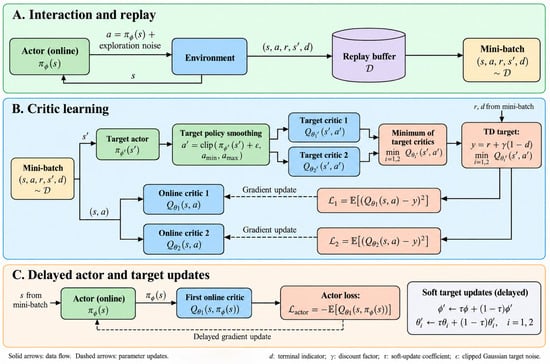
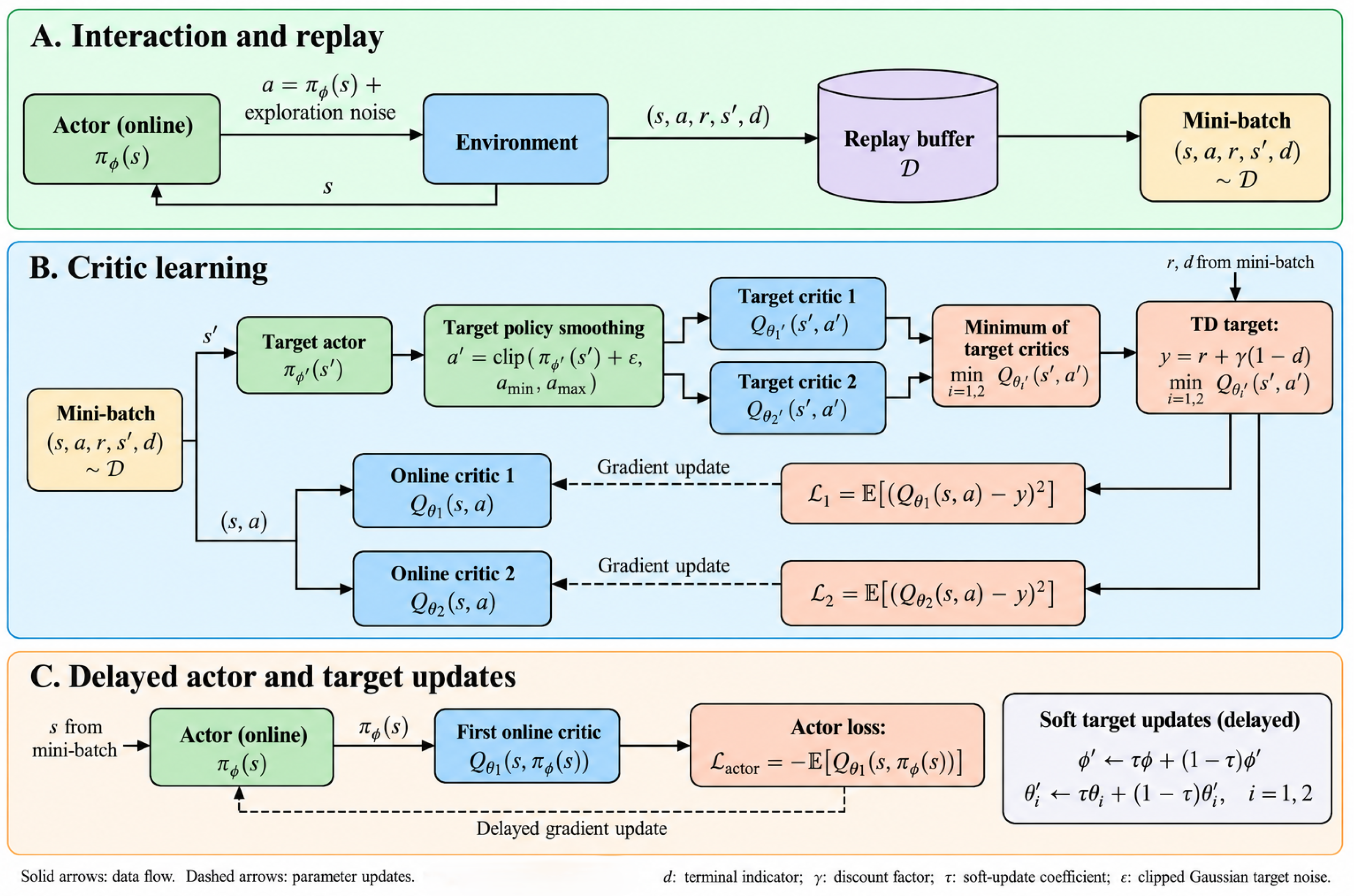
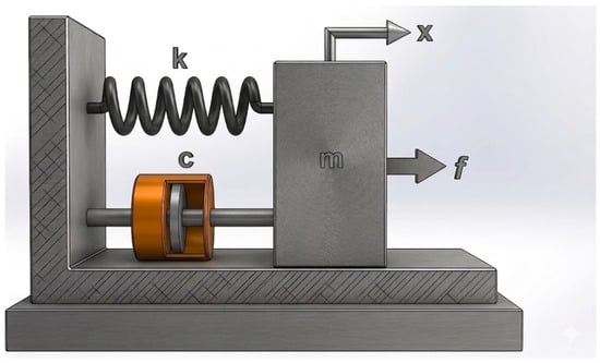
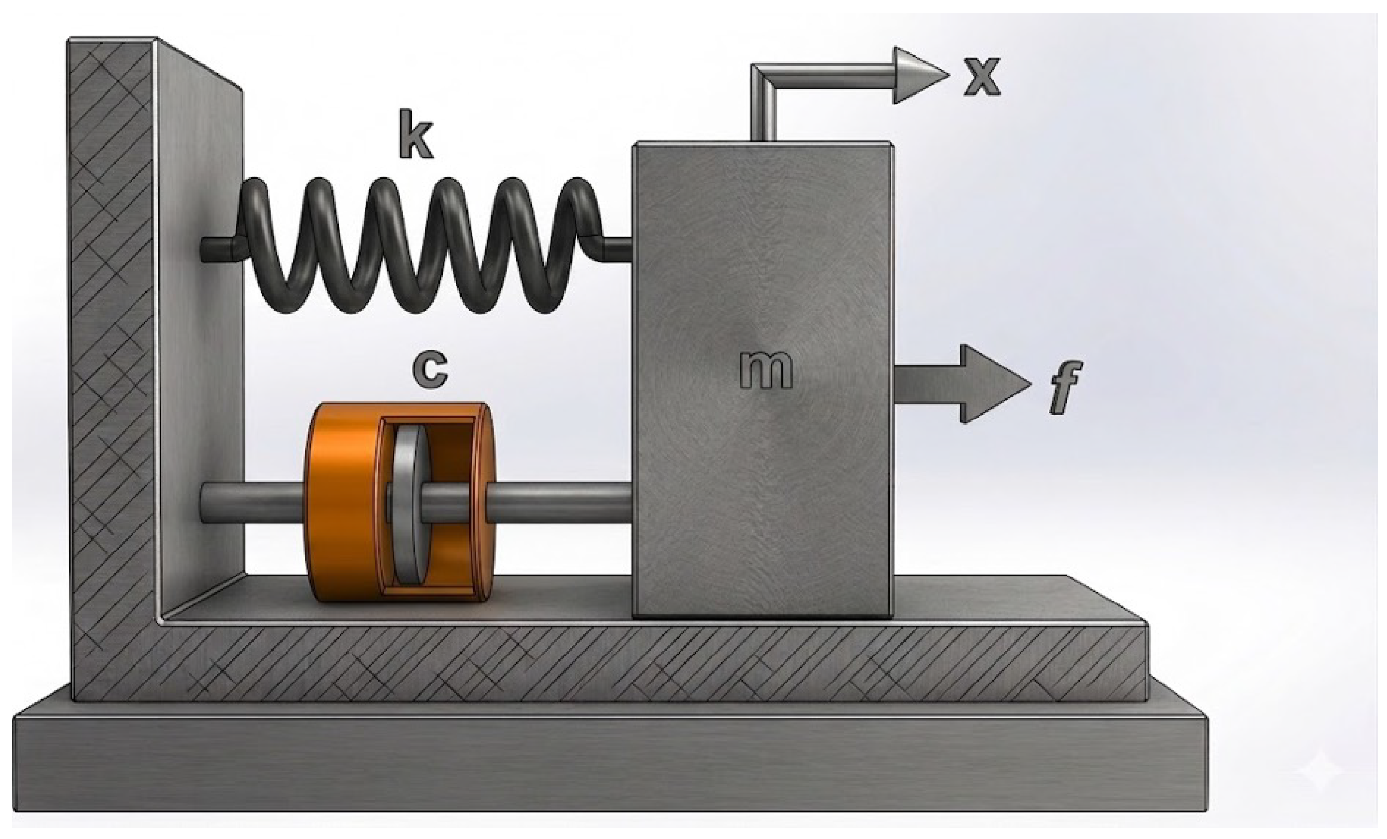
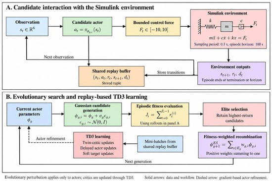
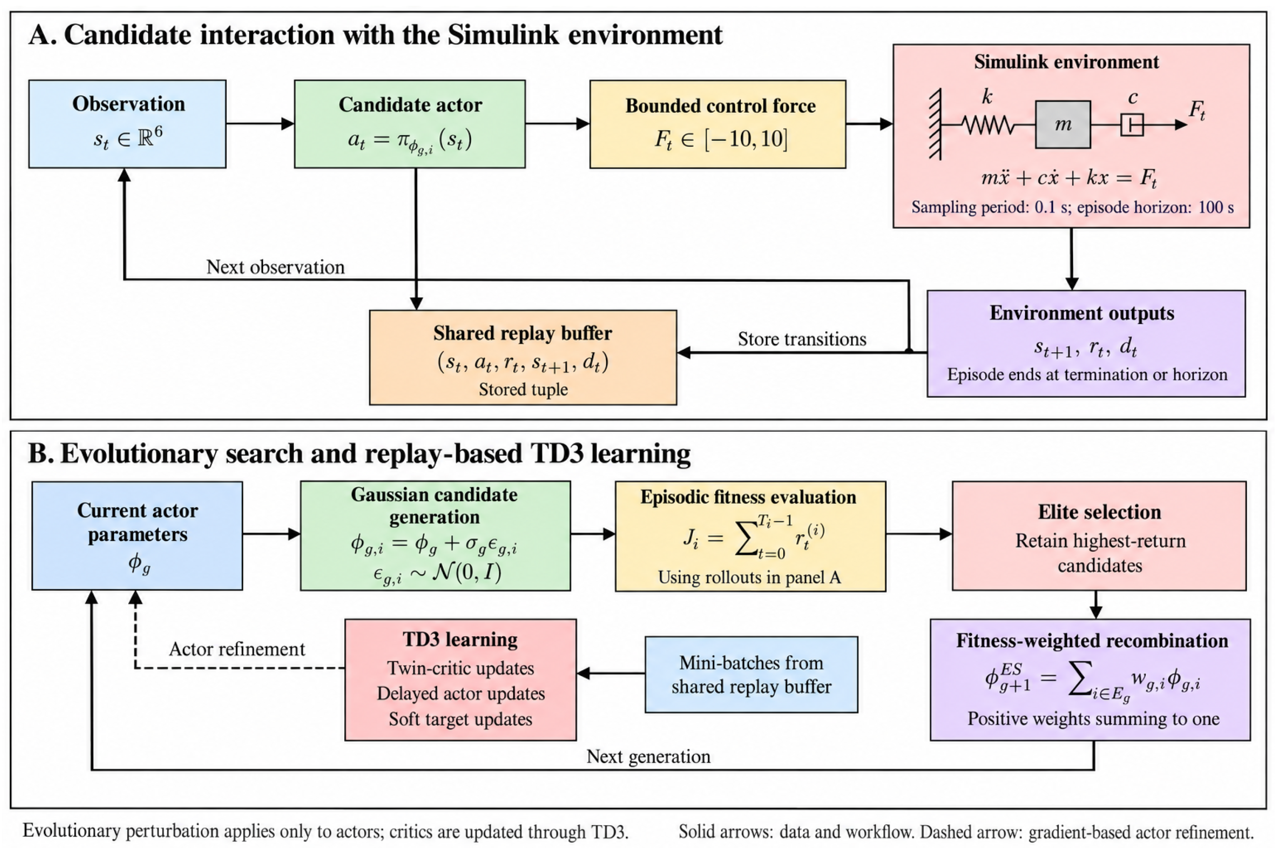
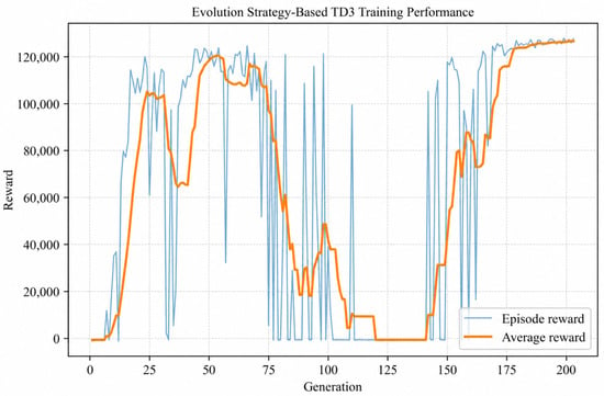
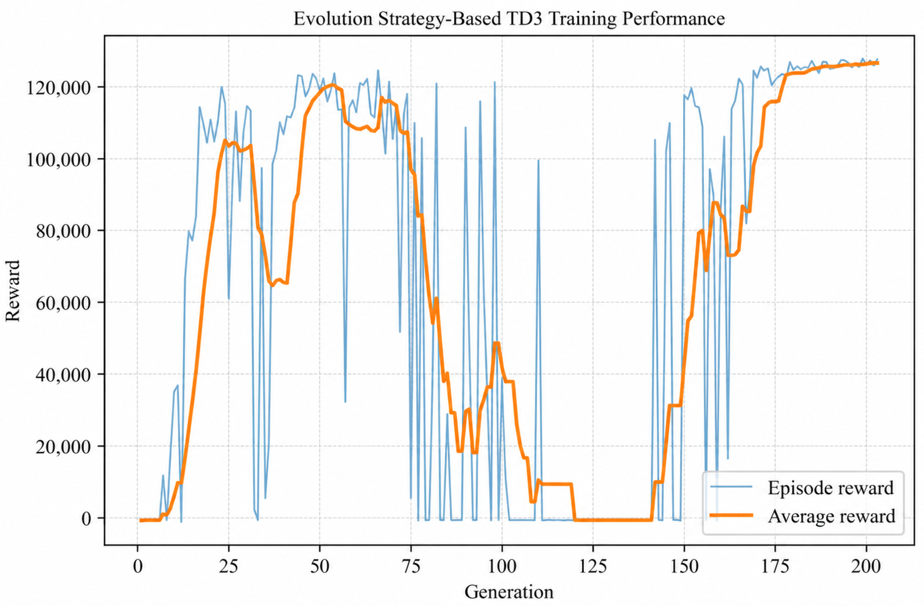
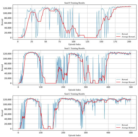
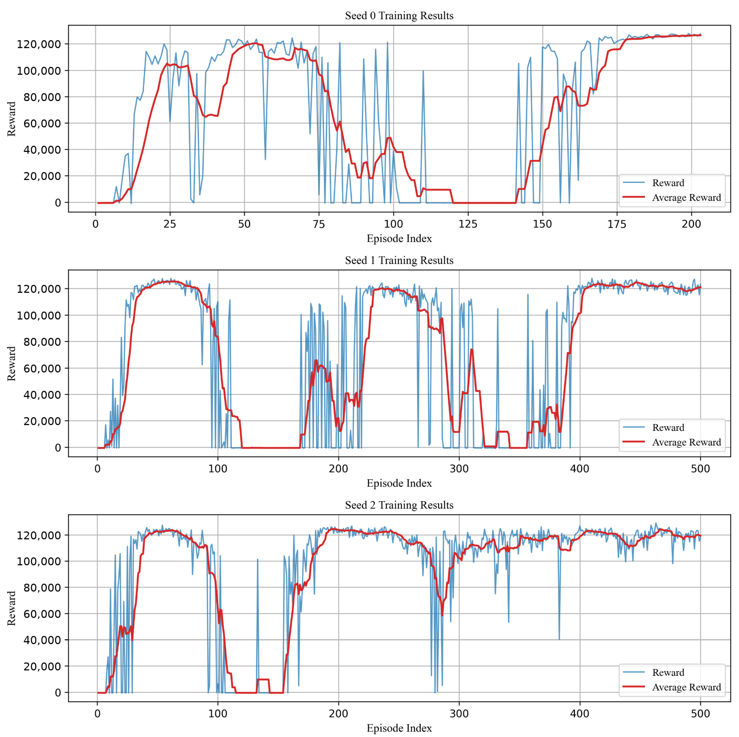
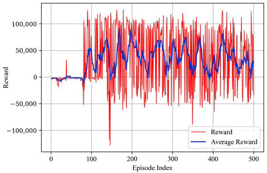
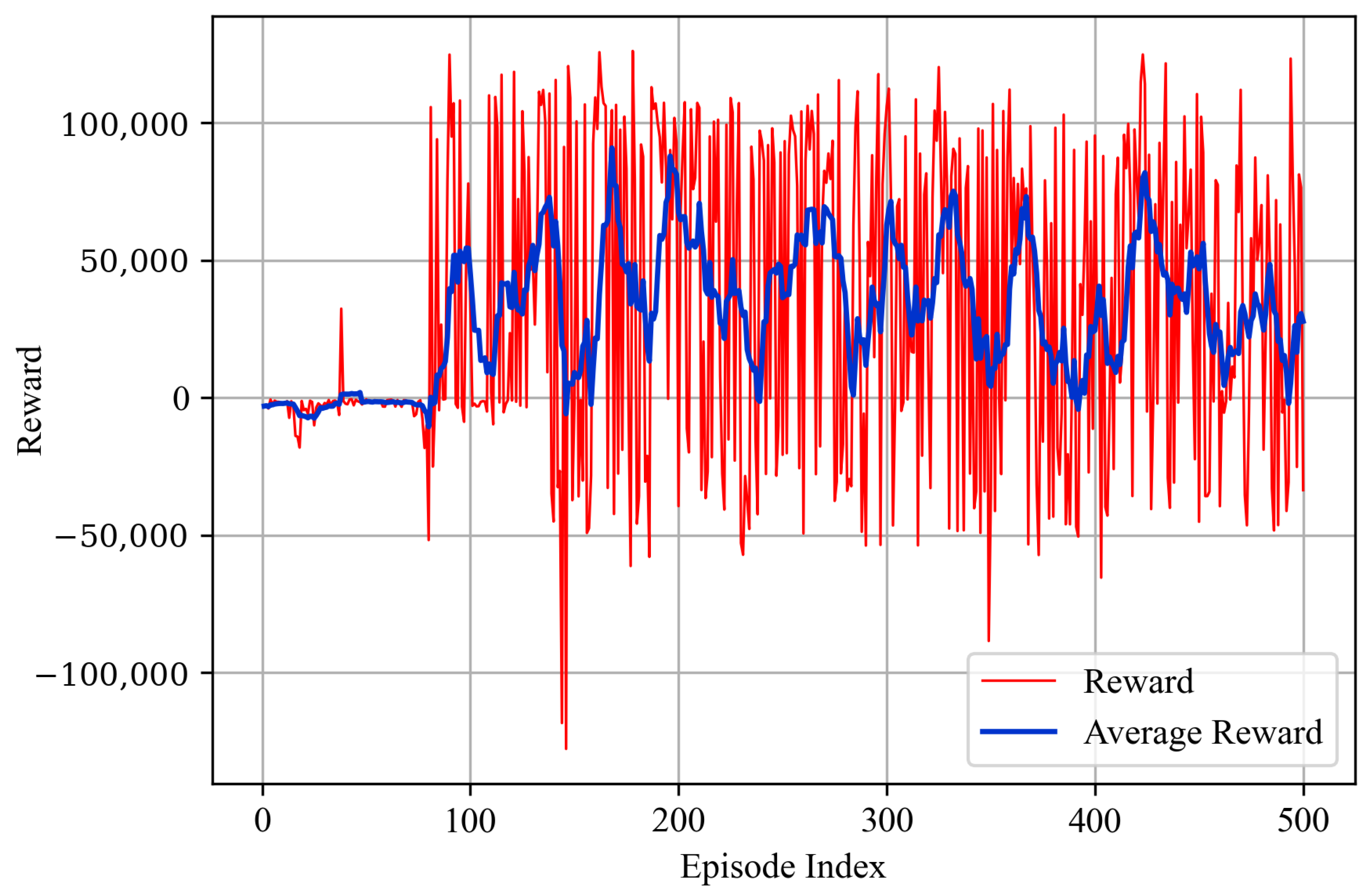
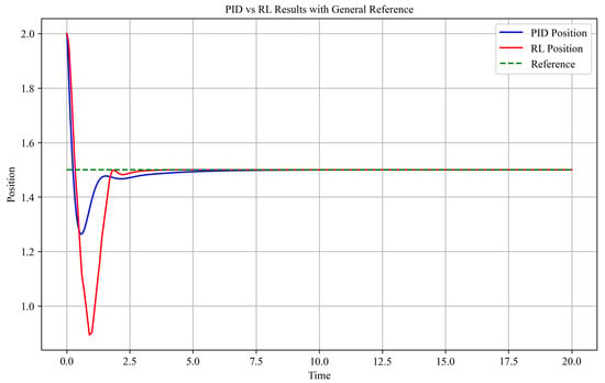
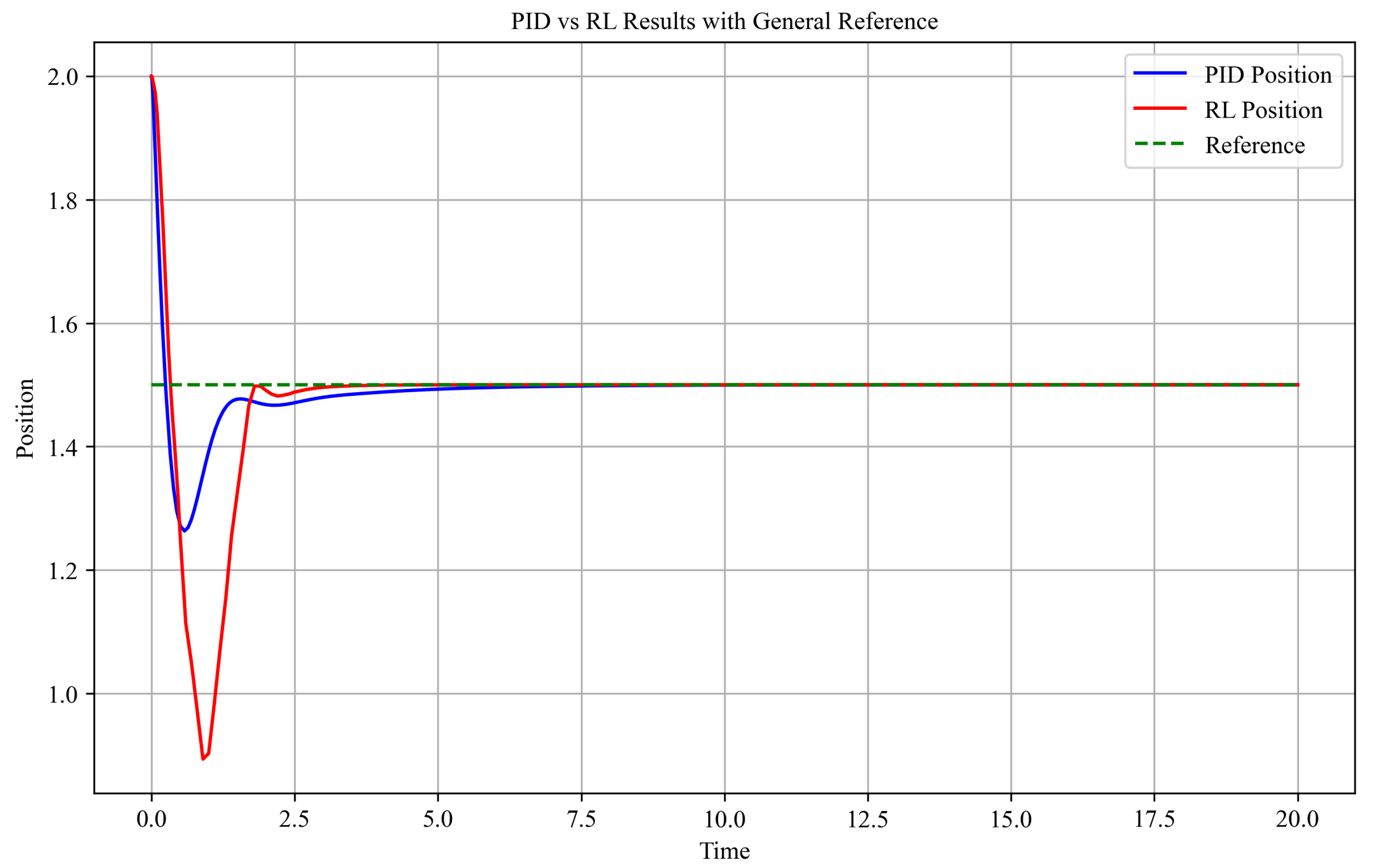
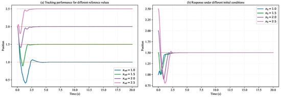
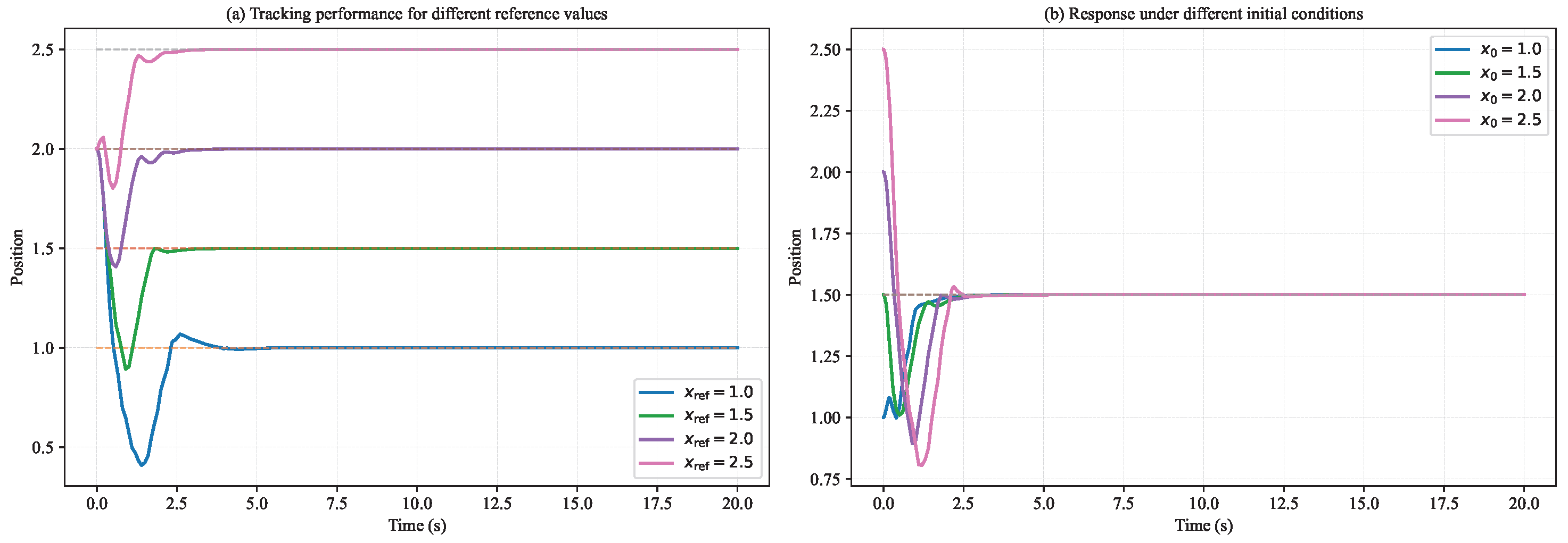

Disclaimer/Publisher’s Note: The statements, opinions and data contained in all publications are solely those of the individual author(s) and contributor(s) and not of MDPI and/or the editor(s). MDPI and/or the editor(s) disclaim responsibility for any injury to people or property resulting from any ideas, methods, instructions or products referred to in the content. |
© 2026 by the authors. Licensee MDPI, Basel, Switzerland. This article is an open access article distributed under the terms and conditions of the Creative Commons Attribution (CC BY) license.